studies in nonlinear dynamics &...

Studies in Nonlinear Dynamics &Econometrics

Volume 16, Issue 4 2012 Article 2

Asset Pricing with Heterogeneous InvestmentHorizons

Mikhail Anufriev∗ Giulio Bottazzi†

∗University of Technology, Sydney, [email protected]†Scuola Superiore Sant’Anna, [email protected]

DOI: 10.1515/1558-3708.1903

Copyright c©2012 De Gruyter. All rights reserved.

Brought to you by | University of Technology SydeyAuthenticated | 138.25.78.25

Download Date | 10/19/12 5:30 AM

Asset Pricing with Heterogeneous InvestmentHorizons∗

Mikhail Anufriev and Giulio Bottazzi

Abstract

We consider an analytically tractable asset pricing model describing the trading activity in astylized market with two assets. Traders are boundedly rational expected utility maximizers withdifferent beliefs about future prices and different investment horizons. In particular, we analyze theeffects of the latter source of heterogeneity on the dynamics of price. We find that in the case withhomogeneous agents, longer investment horizons lead to more stable dynamics. This is not true,however, in the case of a mixed population of traders, when the increase of heterogeneity in theinvestment horizons can introduce instability in the system. Furthermore, the role of heterogeneityturns out to be different for different trading behaviors and its effect on the aggregate dynamicsdepends on the whole ecology of agents’ beliefs.

∗The authors thank Cars Hommes, Alan Kirman and Angelo Secchi for careful reading of previousdrafts and for insightful suggestions which led to a considerable improvement of the paper. Weare grateful to two anonymous referees and the participants of the conferences and seminars inPorto, Kyoto, Amsterdam and Pisa for helpful comments. The usual disclaimers apply. Supportto this research by the Italian Ministry of University and Research (grant E6002GB), Sant’AnnaSchool of Advanced Studies (grant ERIS02GB) and the EU funding within Sixth and SeventhFramework Programmes (FP6-NEST grant 516446, COMPLEXMARKETS and FP7-SSH grant.225408, POLHIA) are gratefully acknowledged.



1 Introduction

In this paper we present a simple, analytically tractable, dynamic modelof speculative market where mean-variance maximizing, boundedly rationalagents trade in a Walrasian equilibrium framework. We use this endogenousasset pricing model to investigate the effect of heterogeneity in individual in-vestment horizons on the aggregate market behavior.

As recognized by many authors, see, e.g., Brock (1997) and Guillaumeet al. (1997), most of the “stylized facts” characterizing the dynamics of finan-cial markets cannot be explained within the standard paradigm of the EfficientMarket Hypothesis (see Fama (1970) for a review). This impossibility has beenthe driving force behind the emergence of a strand of “agent-based” modelswhich describe markets as complex systems of interacting, boundedly rationaland heterogeneous agents. The majority of contributions to the agent-basedliterature is constituted by relatively complex models which are mainly studiedthrough extensive computer simulations, see for instance Levy et al. (1994),Arthur et al. (1997), Lux and Marchesi (1999), Kirman and Teyssiere (2002)and the review in LeBaron (2006). In the same period a second group of sim-ilarly inspired models, the so-called “Heterogeneous Agent Models” (HAMs),emerged. These models typically present simplified frameworks which can bestudied using the mathematical tools of the theory of dynamical systems. Ex-amples of analytically tractable models can be found in the contributions byLux (1995), Brock and Hommes (1998), Gaunersdorfer (2000), Chiarella andHe (2001), Westerhoff and Reitz (2003), Brock et al. (2005), Anufriev et al.(2006), Chiarella et al. (2006), Manzan and Westerhoff (2007) and Anufrievand Bottazzi (2010).

The recent review by Hommes (2006) shows that the literature onHAMs has achieved a considerable success in explaining observed deviationsfrom the Efficient Market Hypothesis. Apart from a few exceptions, however,HAMs focus on only one source of heterogeneity, the heterogeneity in expec-tations. Investors are typically assumed to be “myopic”, so that their demanddepends on the expectations about next period price. Such myopia implies ho-mogeneity both in the time horizon and in the frequency with which investorsoperate in the market. This simplifying assumption is made despite the op-posite evidence that, in real markets, “the variety of time horizons is large:from intra-day dealers, who close their positions every evening, to long-terminvestors and central banks” (Dacorogna et al., 1995). Furthermore, as earlysurvey data on investors’ expectations (Frankel and Froot, 1987b; Ito, 1990)and recent theoretical review (Kirman, 2006) suggest, heterogeneity in timehorizons and heterogeneity in expectations are closely related, with the former

1Anufriev and Bottazzi: Asset Pricing with Heterogeneous Investment Horizons

Published by De Gruyter, 2012Brought to you by | University of Technology Sydey

Authenticated | 138.25.78.25Download Date | 10/19/12 5:30 AM

being plausibly one of the central components of the latter.The question addressed in this paper is whether the predictions of the

HAMs about the possible instability of the price dynamics due to the hetero-geneity in expectations remain equally valid in the presence of traders with dif-ferent investment horizons. Relatedly, our investigation sheds new light on thebroader question of what are the minimal requirements sufficient to generatethe “instability” phenomena observed in financial markets, like the emergenceof bubble and burst dynamics and the persistence of excess volatility. While itis commonly accepted that the heterogeneity of behaviors characterizing thedifferent traders plays a major role in the explanation of these “stylized facts”,the question remains whether heterogeneity in traders’ expectations is neces-sary to generate these phenomena, or, instead, other sources of heterogeneity(e.g., different attitude towards risk, different investment horizons, the extentand quality of available information) can be sufficient.

We analyze the effect of investors’ horizons and their heterogeneityon the aggregate market dynamics within an asset-pricing model proposed inBottazzi (2002). The structure of the model is simple. It is a speculativeeconomy with two assets: a riskless bond and a risky equity whose price isdetermined via a Walrasian mechanism. The market participants maximizea mean-variance utility over their trading horizon but may be heterogeneousin terms of beliefs and preferences. Differently from a majority of HAMs,traders in the model of Bottazzi (2002) build expectations about future pricereturn and not price levels. They also explicitly take into account both theexpected return and the risk involved in their market positions. The relativeshares of different trading behaviors are kept fixed.1 Analysis in Bottazzi(2002) shows that the model with these characteristics can produce non-trivialaggregate price dynamics with sudden bubbles and crashes, when agents haveheterogeneous expectations about return.

Within this framework we introduce two distinct classes of agents, fun-damentalists and chartists, intended to stylize two basic attitudes of marketparticipation. The first class represents traders who obtain future return pre-dictions on the basis of the fundamental value of the asset, while traders be-longing to the second class base their forecasts on the past history of pricereturns. The two groups of traders may differ in their investment horizons.

We show that if agents are homogeneous with respect to their pref-

1The latter assumption can be motivated by the fact that the main players in the financialmarkets are usually led by specific strategies (often dependent on their horizon), whosefrequency of updating is much lower than the frequency of trade. Brock and LeBaron(1996) discuss the issue of different time scales in finance in the context of asymmetricinformation model.

2 Studies in Nonlinear Dynamics & Econometrics Vol. 16 [2012], No. 4, Article 2



erences and the procedures by which they build their expectations, the het-erogeneity in investment horizons cannot destabilize the market. This resulttends to support the view that heterogeneity in expectations is of primaryimportance in generating excess volatility and trading volume. However, wealso demonstrate that when agents do have heterogeneous expectations aboutfuture market behavior, the heterogeneity in time horizons has a strong effecton the aggregate behavior. In particular, the price dynamics turn out to bevery sensitive to the way in which investors extrapolate the estimation of riskover time. We investigate this effect by studying two reasonable, albeit verysimple, procedures for risk extrapolation and by comparing their respectiveeffects on the dynamics of the model. Quite unexpectedly we find that fora relatively large range of parameters, the stability region shrinks with theincrease of the investment horizon of fundamentalists. We argue that the ul-timate reason for this phenomenon lies in the fact that the instability of thesystem is related with the fundamentalists’ relative demand for the risky asset,with respect to the demand of chartists. If the former demand is relativelylow, as it happens when the fundamentalists overestimate the risk, then thesystem becomes unstable.

The rest of the paper is organized as follows. In the next section werecall the importance of time horizon in investor’s financial decision and brieflydiscuss previous contributions. In Section 3 the analytical asset pricing modelis introduced. We discuss the different assumptions on which our model isbased and, in particular, we describe two “stylized” classes of market partic-ipants, fundamentalists and chartists. Despite the simplicity of the model,we try to link the behavioral assumptions behind the definition of these twoclasses to empirical evidence. In this vein, we distinguish between two typesof fundamentalists: sophisticated and unsophisticated. As a first simple ex-ample, in Section 4 we study the model in the special case in which there areno chartists in the market. We show that, in this case, heterogeneity in in-vestment horizons cannot destabilize the market. In Section 5 we perform thestudy of the general case when both fundamentalists and chartists are presentin the market. The analysis of the typical price and wealth dynamics gener-ated by the model is presented in Section 6 while in Section 7 we discuss theimplications of our findings with particular emphasis on the role of time hori-zons. Section 8 contains some final remarks and suggestions on possible futuredevelopments. The proofs of all propositions are provided in the Appendix.




2 Investment Horizons

Any financial advisor nowadays designs the portfolio of every individual clienttaking in consideration the horizon of his or her investment. The individ-ual investment horizons, i.e., the span of time over which agents judge theperformance of their investments, affect their perceived level of risk and, con-sequently, their portfolio choice. Moreover, different types of assets possess,in general, different level of desirability for traders who have long-term needsand for those who have short-term objectives.

Investors who have more than 10 years to invest in the market areusually thought of as those who have long horizon. These investors are typ-ically young professionals or even high school or college students. There isquite strong evidence that financial planners encourage such young investorsto have a portfolio with greater risk compared to other investors, since thesehigher risk portfolios tend also to generate higher market returns over time.In contrast, those investors who are of pre-retiree and retiree status usuallyhave short investment horizons. Investors who have short horizons are gener-ally the least tolerant toward investment risk. They are more concerned withpreserving their existing capital and income. These two classes of investorsjudge risk differently, and so it is not surprising that the optimal choice forthese two groups can be different.

Since the classical financial asset pricing model of Markowitz, Sharpeand Lintner, known as the Capital Asset Pricing Model (CAPM), did notcapture the problem of different horizons in investment decisions, the naturalquestion about its generalization arose in the academic community. Economicintuition would suggest that trading horizons do not affect prices in the worldof fully rational traders, as even short-term speculators have to take into ac-count future expected prices over an infinite time horizon. The intertemporalversions of the CAPM in LeRoy (1973) and Merton (1973), dynamic pricingmodels (Samuelson, 1969; Lucas, 1978) and more recent generalizations (seeCampbell and Viceira (2002) and references therein) provide the conditions un-der which that intuition is correct. These models also offer a number of reasonswhy the optimal portfolio decision might be affected by investment horizons,including the time variations in the market expected returns and agent’s laborincome. However, all these models share extremely strict assumptions aboutthe preference structure of agents and the price generation process. In par-ticular, they share the assumption of an infinitely living representative agenthaving fully rational behavior.

Notwithstanding the simplicity and elegance of such an approach, thenecessity to distinguish between different types of boundedly rational trading




behaviors is now widely acknowledged. Extensive evidence from real markets(Frankel and Froot, 1987a; Allen and Taylor, 1990) suggests that both techni-cal and fundamental analysis play an important role for price determination.This evidence, indeed, was one of the driving forces behind the rise of theheterogeneous agents models mentioned in the previous section. Typically theHAMs ignore the fact that the heterogeneity of trading strategies can be re-lated to differences in traders’ investment horizons. This might be a drawback,because, e.g., simulations of an order-driven market in LiCalzi and Pellizzari(2003) show that the sole difference in planning horizons can lead to a rich setof different outcomes.

For what concerns analytical studies, a number of more traditional con-tributions tried to incorporate differences in trading horizons. For example, themodel in Froot et al. (1992) considers an order-driven market of a single asset.It is based on the idea that short-term traders typically take advantage of thetemporary rise of asset price generated by herding behavior, which, conversely,negatively affects the realized profits of long-term traders. In the model, beforethe trade starts, rational homogeneous speculators have to choose one amongtwo alternative but complementary sources of information about the liquida-tion value of the asset. They then submit their optimal asset demands tothe risk neutral competitive market-makers. It is shown that the equilibriumchoices regarding the information source depend on traders horizons, i.e., onwhether they are going to close their positions before or after the liquidationvalue becomes known. Short term traders prefer to coordinate their choices onone particular source of information. Such herding will lead to a temporary(positive or negative) “bubble” which turns out to be profitable to the major-ity of traders. On the other hand, traders with long horizons prefer efficientinformation, so that they tend to distribute themselves evenly over the twosources of information. By affecting traders expectations, investment horizonsexert a direct effect on prevailing prices.

Osler (1995) makes a step further and considers the situation in whichthe aggregate market behavior endogenously affects the choice of traders’ hori-zons. She presents a Walrasian two-period model in which two equilibria arepossible, with a majority of long- or short-term traders, respectively. The keyassumption for this result is the proportionality between the number of tradershaving a given horizon and the volatility of the market over that horizon. If themajority of traders switch to long horizons, the volatility of long-term returnsdecreases with respect to the short-term volatility, so that long-term traderswill earn a higher risk-weighted expected return. On the other hand, whenthe majority of traders have short horizons, the lower short term volatilityleads to an increase of the short-term traders expected gains. In this model




the aggregate price dynamics are determined simultaneously with the traders’horizons.

Hillebrand and Wenzelburger (2006) extend the traditional CAPM tothe case of overlapping cohorts of investors with linear mean-variance prefer-ences and different planning horizons. They present a rather general theoret-ical framework, but restrict their analysis to the case of “perfect forecastingrules” which is equivalent, in their framework, to rational expectations. In gen-eral, they find that short horizon investors prefer less risky portfolio and thatthe optimal portfolio for investors with different planning horizons is composedof different mixtures of the underlying risky assets.

In the present paper we try to bring the analysis of the effect of invest-ment horizon on price dynamics within the framework of analytically tractableheterogeneous agent models. The dynamic aspect, coming from the presenceof adaptive agents, distinguishes our model from the analysis of Froot et al.(1992), Osler (1995) and Hillebrand and Wenzelburger (2006), where the as-sumption about agents’ rationality allowed to compute static market equilib-ria. We model the demand of agents through mean-variance optimization,allowing for heterogeneity in individual expectations about the first two mo-ments of future returns. In particular, we introduce two classes of agents,fundamentalists and chartists. Even if the model with endogenous investmenthorizons of heterogeneous agents would be an interesting research topic, weshall fix in this paper the horizon for each type and concentrate on the effect ofthe horizons on the price dynamics. There are, however, many different waysin which the trading activity of agents with different investment horizons canbe described.

One can assume, for instance, that an agent with a time horizon of η > 0periods forward does not correct his portfolio between time t, when his decisionabout portfolio is initially made, and time t + η. This agent will participatein the market activity only once each η periods and will choose the desirableamount of risky asset maximizing the expected utility of his portfolio η periodsin the future. This assumption introduces some level of “irrationality” in theagent’s behavior, since the agent is supposed to ignore the information revealedby the trading activity that takes place in the η− 1 trading sessions occurringbetween his consecutive market participations. On the other hand, due to itsrelative simplicity and its low computational requirement, this behavior maynot be unrealistic, especially for individual investors.

Another, rather extreme, possibility is to assume that an agent tradesat each period, continuously correcting his portfolio composition in order tomaximize the utility of future wealth, but taking into account the fact that theportfolio will be revised each period, on the basis of new information. Such an




approach assumes a high level of rationality in agents’ description, and it hasbeen widely used (in continuous-time case) after the seminal paper of Merton(1973). Even inside the representative agent paradigm, however, Merton’smodel is, in general, not analytically tractable. Moreover, the introduction ofa minimal degree of heterogeneity in agents’ behaviors would lead to even morecomplex dynamic programming problems that, in our opinion, would requirea quite unrealistic degree of sophistication from the part of the agents.

In our model we shall follow a different, in a sense intermediate, ap-proach. We assume that an agent with investment horizon η maximizes, atperiod t, his expected wealth at period t + η, without taking into accountthe possibility of future portfolio revisions. However, in each period the agentrevises his portfolio if necessary, i.e., if the new market situation or new indi-vidual expectations lead him to a different optimal portfolio composition. Thisis similar to the strategies of the mutual funds which offer different investmentplans for the specific time periods to individual investors and then operate inthe financial markets on behalf of their clients.2

3 Model Structure

This section provides a detailed description of the formal implementation of themodel. The different parameters are introduced and discussed and the generalpricing equation for an arbitrarily large number of heterogeneous agents isobtained. Next, we introduce two special classes of traders, chartists andfundamentalists, and derive the reduced-form pricing equation which describesthe dynamics of the model when only these types of agent are present in themarket.

3.1 Market Dynamics

Consider a simple pure exchange economy with two goods: a riskless security(bond) that gives a constant interest rate rf > 0 and a risky security (equity)that pays a positive dividend at the beginning of each period t. For the sakeof simplicity we assume that the dividend is constant3 and denote it as D.

2Alternatively, our model can by formally presented as an overlapping generation modelwhere, for any horizon η, there exist η generations of traders who revise their positions everyη periods.

3The qualitative aspects of the model will be the same when the dividend is an i.i.d. ran-dom variable with moderately small variance (see Bottazzi (2002) for the details). In Sec-tion 6 we show the results of numerical simulations with random dividend and discuss theeffect of the stochastic components on the aggregate dynamics.




This assumption is satisfied, for example, in the bond market where the fixedcoupon payment plays the role of the dividend.

The riskless asset is assumed to be the numeraire of the economy andits price is fixed to 1. The price of the risky asset Pt is determined each periodby market clearing. The fundamental price of the risky asset P is defined asthe discounted stream of expected dividends

P =∞∑t=1

D

(1 + rf )t=

D

rf. (1)

We also denote as ρt,t+η the price return of the risky asset between time t andtime t+ η,

ρt,t+η =Pt+η − Pt

Pt

=

t+η−1∏τ=t

(1 + ρτ,τ+1)− 1 .

Assume the economy is populated by N heterogeneous traders and letWt,n be the wealth of agent n (1 ≤ n ≤ N) at time t. The investment decisionof the n-th agent is described as the share xt,n of the personal current wealthinvested in the risky asset. If ηn is the investment horizon, the decision will bebased on the distribution of agent’s wealth ηn periods in the future, Wt+ηn,n.Assuming that the earned dividends are fully reinvested in the riskless assetone has

Wt+ηn,n(Pt, ρt,t+η) =

(1− xt,n)Wt,n (1 + rf )ηn + xt,nWt,n

(1 + ρt,t+ηn +

Dηn

Pt

),

(2)

where Dη stands for the stream of dividends earned in η periods, augmentedby the received riskless interests

Dη =

η−1∑τ=0

D (1 + rf )τ = P

((1 + rf )

η − 1).

At each period t, and for any notional price P , the n-th agent will choosethe share of wealth invested in the risky asset, x∗

t,n, to maximize the expectedmean-variance utility of the future wealth (2), so that

x∗t,n(P ) = argmax

xt,n

{Et,n

[Wt+ηn,n(P, ρt,t+η)

]−

− βn

2Vt,n

[Wt+ηn,n(P, ρt,t+η)

]},

(3)




where Et,n[·] and Vt,n[·] stand, respectively, for the expected mean and varianceof their argument obtained by agent n using the information available at timet, and βn is the risk aversion parameter of agent n.

The intertemporal dynamics of the model proceeds as follows. At thebeginning of period t agent n possesses At−1,n shares of the risky and Bt−1,n

shares of the riskless asset. First, all agents receive dividends per every ownedshare of the risky asset and interest rate on owned riskless securities. Theseearnings are paid in terms of the numeraire. Then using (3) each agent com-putes the desired amount of the risky asset At,n(P ) for any notional price

At,n(P ) =x∗t,n(P )Wt,n(P )

P. (4)

Finally, the prevailing price of the risky asset Pt is fixed using the marketclearing condition

N∑n=1

At,n(Pt) = At , (5)

where At is the number of outstanding shares of the risky security at timet. Alternatively, one can compute the individual excess demand function∆At,n(P ) = At,n(P )− At−1,n of agent n and fix the price of the asset using

N∑n=1

∆At,n(P ) = ∆At , (6)

where ∆At = At − At−1 is the “outside” supply of the risky shares at timet. Equations (5) and (6) are equivalent and establish, at the same time, thepresent price Pt of the risky asset and the present composition of each portfolio,agent n owningAt,n = At,n(Pt) risky andBt,n = Pt∆At,n+At−1,nD+Bt−1,n (1+rf ) riskless shares. At this point, once prices and allocations are decided, if themarket behavior in terms of price and returns did not change, agent n wouldavoid to trade in the market until period t + ηn. However, new informationabout realized prices may (and generally will) force the agent to change thedesirable amount of the risky asset and, consequently, the composition of hisportfolio, before the notional maturity of its present investment. Nonetheless,contrary to the dynamical programming approach, agents in our model do nottake into account (and do not anticipate) their future actions. In this sense,our agents are boundedly rational.




3.2 Pricing Equation

In order to solve (3), agents have to form expectations about their wealthat future time. The only source of uncertainty is constituted by the returnρt,t+ηn . Let Et,n[ρt,t+ηn ] and Vt,n[ρt,t+ηn ] be the expectation of agent n aboutthe average value of price return and its variance, respectively. Then from (2),the conditional distribution of future wealth Wt+ηn,n, given current price Pt

and wealth Wt,n, has the following expected value and variance

Et,n[Wt+ηn,n] = Wt,n (1 + rf )ηn+

+ xt,nWt,n

(Et,n[ρt,t+ηn ] +Rηn(P /P − 1)

)Vt,n[Wt+ηn,n] =

(xt,nWt,n

)2Vt,n[ρt,t+ηn ] ,

(7)

where P stands for the fundamental price of the risky asset introduced in (1),and Rη = (1+ rf )

η − 1 for the positive return gained from holding the risklessasset during η periods. Plugging (7) in (3), solving the optimization problemand substituting the result in (4), one obtains

At,n(P ) =Et,n[ρt,t+ηn ] +Rηn(P /P − 1)

βn P Vt,n[ρt,t+ηn ]. (8)

Notice that if P = P and Et,n[ρt,t+ηn ] = 0, that is if the initial price of the riskysecurity is equal to its fundamental value and no price change is predicted, andif the forecasted variance is positive Vt,n > 0, then the desirable amount ofthe risky asset in portfolio is equal to zero. This is as expected, since in thissituation the risky security pays the same return as the riskless one and is, forany level of risk, less desirable. More generally, the desirable amount of riskyasset is proportional to the excess return and inversely proportional to theexpected risk. It also decreases with the current price P and with agent’s riskaversion coefficient βn. Inside the previous expression the investor’s horizon ηnappears in three distinct places: it affects the expected excess return and theexpected variance, since they both have to be computed over ηn periods, andit contributes to the wealth accumulation through the dividend re-investmentaccounted for by the term Rηn .

Starting from the amount of asset desired by each agent n at any pricelevel P the prevailing price is finally computed using (5) (or equivalently (6)).Assuming that the outstanding number of shares is constant At = ATOT , ∀tand substituting (8) in (5) one obtains

A =1

N

N∑n=1

Et,n[ρt,t+ηn ]−Rηn

βnVt,n[ρt,t+ηn ]

1

P+

1

N

N∑n=1

P Rηn

βnVt,n[ρt,t+ηn ]

1

P 2, (9)




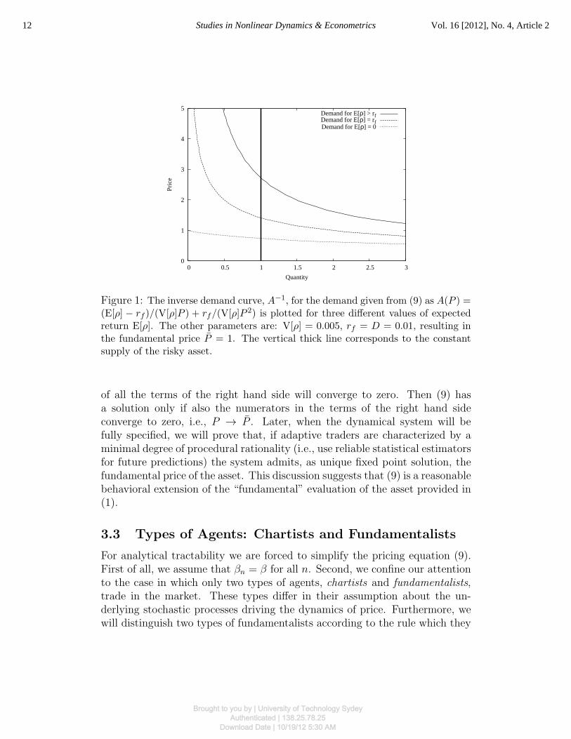
where A = ATOT/N stands for the number of risky shares per investor. Thetwo coefficients on the right hand side of (9) are population averages of dif-ferent quantities. The numerator of the first summand is the expected excessreturn of the capital gain of the risky asset, while the numerator of the secondsummand represents the capital which agent n obtains from the stream of div-idends payed by the risky asset over ηn periods. Both quantities are weightedby the risk factor 1/ (βnVt,n[ρt,t+ηn ]), which accounts for the agents’ personalevaluation of the risk implied in keeping the risky stock in the portfolio. SinceP > 0, the second term in the right hand side of (9) is positive. Together withthe positiveness of A, this implies the existence and uniqueness of the posi-tive solution of the quadratic4 equation (9). This solution defines the marketprice Pt in period t. The market price increases with the average risk-weightedexpected capital gain and with the payed dividend and decreases with the rel-ative supply of the asset and with the increase of the forecasted risk. In Fig. 1the price determination is illustrated when the horizon η = 1 and the expec-tations are homogeneous, i.e., when βn = 1, Rηn = rf , Et,n[ρt,t+ηn ] = E[ρ]and Vt,n[ρt,t+ηn ] = V[ρ] for all n and t. Three demand curves for differentvalues of the expected return E[ρ] are reported. Notice that if E[ρ] = 0, themarket clearing price is below the fundamental level P . This is because theagents expect positive fluctuations and require a risk premium for holding apositive amount of shares in the market equilibrium. If the agents expectedzero fluctuations, the inverse demand function would become flat, resultingin the intersection with supply at P = P = 1 and the risk premium woulddisappear.

The latter fact is an important property of (9) and can be demonstratedin general case. Assume that the price of the asset fluctuates randomly arounda constant level. Then, if all agents use unbiased estimators to predict futureprice returns, the investment horizon has no effect on the forecast of expectedreturns and Et,n[ρt,t+ηn ] = 0, for all n. With this assumption, Eq. (9) reducesto

A =1

N

N∑n=1

Rηn

βnVt,n[ρt,t+ηn ]

P − P

P 2.

If the fluctuations around the constant price level get smaller and the agentsuse consistent and unbiased estimators for the variance, the denominators

4The non-linear pricing equation (9) can be contrasted with the linear pricing equationobtained in Brock and Hommes (1998) starting from very similar assumptions. The differ-ence resides in our assumption that agents form expectations about future return, not price,and in the special choice made in that paper to set ATOT = 0.




0

1

2

3

4

5

0 0.5 1 1.5 2 2.5 3

Pric

e

Quantity

Demand for E[ρ] > rfDemand for E[ρ] = rfDemand for E[ρ] = 0

Figure 1: The inverse demand curve, A−1, for the demand given from (9) as A(P ) =(E[ρ] − rf )/(V[ρ]P ) + rf/(V[ρ]P 2) is plotted for three different values of expectedreturn E[ρ]. The other parameters are: V[ρ] = 0.005, rf = D = 0.01, resulting inthe fundamental price P = 1. The vertical thick line corresponds to the constantsupply of the risky asset.

of all the terms of the right hand side will converge to zero. Then (9) hasa solution only if also the numerators in the terms of the right hand sideconverge to zero, i.e., P → P . Later, when the dynamical system will befully specified, we will prove that, if adaptive traders are characterized by aminimal degree of procedural rationality (i.e., use reliable statistical estimatorsfor future predictions) the system admits, as unique fixed point solution, thefundamental price of the asset. This discussion suggests that (9) is a reasonablebehavioral extension of the “fundamental” evaluation of the asset provided in(1).

3.3 Types of Agents: Chartists and Fundamentalists

For analytical tractability we are forced to simplify the pricing equation (9).First of all, we assume that βn = β for all n. Second, we confine our attentionto the case in which only two types of agents, chartists and fundamentalists,trade in the market. These types differ in their assumption about the un-derlying stochastic processes driving the dynamics of price. Furthermore, wewill distinguish two types of fundamentalists according to the rule which they




adopt to extrapolate the prediction of the next period return and varianceover longer time horizons. Below we specify, for each group, how expectationsabout the mean and variance of future returns are formed.

3.3.1 Chartists

Chartists predict returns on the basis of the past returns history using con-sistent statistical estimators. More precisely, at period t, they assume thatthe next price return is equal to the exponentially weighted moving average(EWMA) of past returns, based upon past price realizations up to Pt−1, anddenoted with yt−1, Analogously, for predicting the next period variance theycompute the EWMA estimator of historical variances, denoted with zt−1. TheEWMA estimators yt−1 and zt−1 read

yt−1 = (1− λ)∑∞

τ=2λτ−2ρt−τ ,

zt−1 = (1− λ)∑∞

τ=2λτ−2[ρt−τ − yt−1]

2 .(10)

The parameter λ ∈ [0, 1) measures the relative importance agents put ondifferent past observations: the last available return has the highest weight,while the weights of previous realized returns decline geometrically in the past.One can interpret λ as a “memory” parameter: the higher the value of λ is,the less the recent observations weigh. In the extreme case, when λ = 0, theagent’s memory is the shortest possible and the last realized return is used aspredictor of the next return. This is the case of “naıve” expectations. Noticethat expressions above are analogous to the ones proposed by the RiskMetricsGroupTM (J.P.Morgan, 1996), and widely applied by real operators in theirforecasting activity.5 In what follows we will use the recursive form of theprevious two equations, namely

yt−1 = λyt−2 + (1− λ)ρt−2 ,

zt−1 = λzt−2 + λ (1− λ) (ρt−2 − yt−2)2 .

(11)

Equations (11) describe a one period ahead forecast. To build a long-termforecast, chartists assume that future price dynamics can be described as ageometric random walk. Then the forecasts for both the expected return and

5The RiskMetrics GroupTM group actually proposes an EWMA estimator of the volatil-ity, defined as the second moment of the returns distribution. The expression above repre-sents its natural extension to the central moment.




variance over η periods can be simply obtained multiplying the one-periodforecast by a factor η, to read

EC

t [ρt,t+η] = η EC

t [ρt,t+1] = η yt−1 (12)

and

VC

t [ρt,t+η] = η VC

t [ρt,t+1] = η zt−1 , (13)

where symbols EC

t and VC

t denote the corresponding expectations of chartists.The individual demand function of a chartist can then be obtained from (8)and reads

AC

t (P ) =1

P

yt−1

βzt−1

+P − P

P 2

BC(η)

βzt−1

, (14)

where the term

BC(η) =(1 + rf )

η − 1

η(15)

accounts for the dependence of the demand function on the horizon η.

3.3.2 Fundamentalists

Fundamentalists believe that the price is governed by a process which con-stantly reverts to the fundamental value P : if the asset is presently underval-ued, its price will increase, and if it is overvalued, the price will fall. Moreprecisely, they expect that the future price Pt+1 will be, on average, betweenthe current price Pt and the fundamental price P

EF

t [Pt+1] = Pt + θ (P − Pt) , (16)

where θ ∈ [0, 1] describes the belief of fundamentalists about market reactivityin recovering the fundamental price.6 When θ = 0 equation (16) gives the so-called “naıve” expectations EF

t [Pt+1] = Pt, while θ = 1 corresponds to thecase when fundamentalists believe that the fundamental value will be alreadyreached in the next period. The expression of the multi-steps expected returnunder the assumption of mean-reverting market dynamics reads

EF

t [ρt,t+η] =(1− (1− θ)η

)( P

Pt

− 1

). (17)

6In contrast to the chartists’ behavior, price Pt is included in the information set offundamentalists. Such asymmetry simplifies computations and is not crucial for our results.




This result can be straightforwardly obtained by the recursive use of equation(16).

Since the volatility of the asset is determined essentially by the opinionof the market, we assume that fundamentalists forecast the one period aheadvolatility in the same way as chartists. Thus, VF

t [ρt,t+1] = zt−1, where zt−1 isgiven in (10).

At this stage, it remains to specify the fundamentalists’ forecast VF

t [ρt,t+η]for the variance of return over η periods. For this purpose we introduce twodifferent types of fundamentalists. We refer to one type as sophisticated funda-mentalists and to the other type as unsophisticated fundamentalists, accordingto the complexity of the analytic tools which they use to compute their forecastabout future variance.

Unsophisticated Fundamentalists. These agents implement a relativelysimple reasoning, assuming like chartists that the variance of return linearlyincreases with time

VUF

t [ρt,t+η] = η VF

t [ρt,t+1] = η zt−1 . (18)

On one hand, as we will show below, this assumption about fundamentalists’forecast contradicts to the expectations about price behavior in (16). On theother hand, this specification of the variance corresponds to the behavior com-monly found among financial investors who tend to use fundamental evaluationin judging different investment opportunities while preferring an econometric(technical) approach for the evaluation of the associated risk. Moreover, theBrownian scaling of the volatility described in (18) is qualitatively similar tothe one actually found for real markets (Dacorogna et al., 2001).

The individual demand function of an unsophisticated fundamentalistcan then be obtained from (8) and reads

AUF

t (P ) =P − P

P 2

BUF(η, θ)

βzt−1

, (19)

where the term

BUF(η, θ) =(1 + rf )

η − (1− θ)η

η(20)





Sophisticated Fundamentalists. These fundamentalists forecast futurereturns variance in a way which is consistent with their return expectations(17). They believe that (16) describes the price dynamics in each period. Thisassumption allows them to model the forecast of time series of future returnsas a mean reverting stochastic process. In Appendix A we derive the Fokker-Planck equation that describes the evolution of the long-horizon forecast andwe show that, first, the prediction for the long-term return satisfies (17), and,second, that the long-term asset volatility forecast can be obtained from theone-period volatility forecast VF

t [ρt,t+1] = zt−1 according to the formula

VSF

t [ρt,t+η] =1− (1− θ)2η

θ(2− θ)zt−1 . (21)

The crucial difference between (18) and (21) consists in the fact that the formerinfinitely increases with fundamentalists’ investment horizon η, while the latterconverges to the asymptotic value zt−1/(θ(2− θ)). Thus, on longer investmenthorizons, unsophisticated fundamentalists overestimate risk. We will see laterthat this difference leads to crucial change in the dynamics of the model.

Finally, the individual demand function of sophisticated fundamental-ists can be obtained from (8) and reads

ASF

t (P ) =P − P

P 2

BSF(η, θ)

βzt−1

, (22)

where the term

BSF(η, θ) =((1 + rf )

η − (1− θ)η) 1− (1− θ)2

1− (1− θ)2η(23)


The specification of sophisticated fundamentalists behavior concludesthe building of our artificial market model. In what follows we analyze theeffects of the investment horizons on the aggregate dynamics. For this purposewe present different models based on the previous assumptions, characterizedby an increasing degree of complexity: in the next section we analyze the caseof market without chartists and later, in Section 5, we will extend the analysisto the situation in which both chartists and fundamentalists participate themarket.




4 Market without Chartists

This section is devoted to the simplified model in which the market is popu-lated only by fundamentalists. We explicitly provide the analysis for the casewhen all fundamentalists are unsophisticated. One can easily check that ourresult does not change in the case of sophisticated fundamentalists.

4.1 Homogeneous Investment Horizons

Let us start with the simplest situation and assume that all unsophisticatedfundamentalists in the market have the same forecasting parameter θ and thesame horizon η. Substituting the demand function (19) in (9) the price of therisky asset Pt is determined as the positive root of

P 2 βA zt−1 + (P − P )BUF(η, θ) = 0 , (24)

which reads

Pt =−r +

√r2 + 4 r P γ zt−1

2 γ zt−1

, (25)

where the following parameters have been introduced

γ = βA ,r = BUF(η, θ) .

(26)

Using the pricing equation (25) and the recursive definition of estimators (11)the 3-dimensional system describing the dynamics of the market in terms ofthe scaled price pt = γ Pt reads

pt+1 = f(zt) =−r +

√r2 + 4szt2 zt

yt+1 = λyt + (1− λ)

(f(zt)

pt− 1

)zt+1 = λzt + λ (1− λ)

(f(zt)

pt− 1− yt

)2

,

(27)

where s = rγP . One has the following

Proposition 4.1. The system in (27) has only one fixed point (γP , 0, 0) corre-sponding to the fundamental price of the risky asset. This fixed point is locallyasymptotically stable for all λ < 1.




Proof. See Appendix B.

We run an extensive set of simulations with different parameter valuesand different initial conditions and we conjecture that the point (γP , 0, 0) is,probably, even globally stable.

Notice that a variation of η leads to changes in the value of the parame-ter r, and hence in the value of s, but does not modify the system itself. Thus,the price converges to the fundamental value independently of the investmenthorizon. The speed of convergence to the fixed point depends, however, on η.

4.2 Heterogeneous Investment Horizons

Consider now the market composed of K groups of traders. Each group i ∈{1, . . . , K} is composed by Ni fundamentalists with a forecasting parameter θiand an investment horizon equal to ηi. If we denote the population shares ofthe different groups as fi = Ni/N , where N =

∑Ki=1 Ni, the market clearing

condition becomes

P 2 β A zt−1 + (P − P )K∑i=1

fi BUF(ηi, θi) = 0 . (28)

There is an obvious similarity between (24) and (28). The dynamics of thesystem are still described by (27) with the only difference that the parameterr now reads

r =K∑i=1

fiBUF(ηi, θi) . (29)

Then, in the case of many groups of fundamentalists with different investmenthorizons, the asymptotic behavior of the system remains the same and theprice converges to the fundamental value. In other words, in the market withfundamentalists, the heterogeneity in the investment horizons does not affectthe stability of the system.

In this section we have shown that the presence of groups of funda-mentalists with different time horizons changes the values of the parametersof the dynamical system but does not affect its qualitative behavior. Thus, wecan conclude that there are no qualitative differences between the case withhomogeneous (with respect to the investment horizons) fundamentalists andthe case with heterogeneous ones. In both cases the price converges to thefundamental value and the expectation about future variance goes to zero.




This result reminds a classical result in financial economics, obtainedusing a completely different approach. The solution of the dynamic program-ming model with homogeneous expectations and under a specific assumptionabout preferences (power utility function) in Merton (1973) shows that theoptimal choice of the investor, in each period, does not depend on his invest-ment horizon. This implies that the dynamics of the model remains the samewhen populated by agents with different horizons. We reach the same qual-itative conclusions, using a different utility function and in the presence ofheterogeneous, boundedly rational agents.

5 Complete Model: Fundamentalists vs.

Chartists

Below we derive the deterministic system describing the dynamics of marketwhere both fundamentalists and chartists are present. We start with the casewhen all fundamentalists are non-sophisticated and then move to the case withsophisticated fundamentalists.

5.1 Unsophisticated Fundamentalists

Let us consider the market composed of N1 unsophisticated fundamentalistswith horizons η1 and homogeneous forecasting parameter θ, characterized byindividual demand (19), and N2 chartists with horizons η2 and whose demandfunction is given by (14). Denote as f1 and f2 the fractions of fundamentalistsand chartists, respectively, and assume that all investors in the market havethe same parameter λ. The market clearing equation reads

P 2 β A zt−1 + P(f1B

UF(η1, θ) + f2BC(η2)− f2yt−1

)−

− P(f1B

UF(η1, θ) + f2BC(η2)

)= 0 .

(30)

The positive root of this equation, together with (11), completely define thedynamics of the system. Introducing γ = βA/f2 and

r =f1f2

BUF(η1, θ) +BC(η2) , (31)




the 3-dimensional system for the evolution of the rescaled price p(t) = γPt

reads

pt+1 = g(yt, zt) =(yt − r +

√(yt − r)2 + 4szt

)/2zt

yt+1 = λyt + (1− λ)(g(yt, zt)

pt− 1

)zt+1 = λzt + λ(1− λ)

(g(yt, zt)pt

− 1− yt

)2

,

(32)

where, as in (27), s = rγP . Notice that (32) coincides with the system inBottazzi (2002) derived under the assumption of myopic agents. One has thefollowing

Proposition 5.1. The system in (32) possesses an unique fixed point (γP , 0, 0).This point is locally asymptotically stable if

r + λ > 1 . (33)

When the inequality changes its sign, the complex eigenvalues of the Jacobiancross the unit circle, so that the system exhibits a Neimark-Sacker bifurcationand locally stable quasi-periodic cycles emerge.

Proof. See Appendix C in Bottazzi (2002).

Notice that the presence of chartists does not change the fixed point so-lution of the system, so that at equilibrium the price of the risky asset standsagain on the fundamental level. In general, when the value of λ and/or rdecreases, the system loses stability. Thus, a reduction of the effective “mem-ory” of chartists tends to destabilize the system. At the same time, since∂rfB

UF, ∂rfBC > 0 and r in (31) is increasing with BUF and BC, an increase

of the riskless interest rate tends to stabilize it. The effect of the horizonparameters will be analyzed in Section 7.

5.2 Sophisticated Fundamentalists

It is easy to check that when fundamentalists in the market are sophisticated,i.e., when they use (21) instead of (18) to predict future variance, the pricingequation is very similar to the one obtained in the previous case. The onlydifference is that the coefficient BUF in replaced by BSF. The dynamical systemdescribing the evolution of price is still given by (32), but the parameter r nowreads

r =f1f2

BSF(η1, θ) +BC(η2) . (34)




5.3 Generalization to Many Groups

The generalization to many groups of fundamentalist traders is straightfor-ward. Let us consider a market populated by K1 groups of unsophisticatedfundamentalists, K2 groups of sophisticated fundamentalists and a group ofchartists. We denote with fc the population share of chartist traders and withfi with i ∈ {1, . . . , K1 +K2} the relative shares of the different groups of fun-damentalists (i.e., the number of fundamentalists of group i over the numberof chartists). Let ηc, θi and ηi for i ∈ {1, . . . , K1 + K2} denote the behav-ioral parameters of chartists and of the different groups of fundamentalists,respectively. Then, the dynamics of the system is still described by (32) withγ = βA/fc and

r =

K1∑i=1

fi BUF(ηi, θi) +

K1+K2∑i=K1+1

fi BSF(ηi, θi) +BC(ηc) . (35)

Summarizing, we have shown that irrespectively of the number andtype of fundamentalists, when chartists are present, the market dynamics isdescribed by (32), and Proposition 5.1 applies.

6 Price and Wealth Dynamics

As shown in the previous section, the fundamental price of the risky assetremains a fixed point of the system irrespectively of the kind of agents consid-ered, chartists, unsophisticated or sophisticated fundamentalists. Converselythe stability conditions of this fixed point depend on the different tradingbehaviors. The qualitative behavior of system (32) is studied at length in Bot-tazzi (2002). In general, depending on parameter values and initial conditions,it can display convergence to a fixed point, quasi-cyclic or chaotic behavior.

As an example, in Fig. 2 we plot the long run price dynamics obtainedwith different sets of parameters (see caption). In the benchmark case (whenall agents have investment horizons equal to one, i.e., η1 = η2 = 1) price con-vergences to the fundamental value. The increase of the investment horizon offundamentalists destabilizes the fundamental equilibrium. This plot illustratesalso one of the typical non-converging patterns of price generated by system(32) – price follows quasi-periodic behavior: after relatively slow rise pricesuddenly falls. This behavior reminds the crashes after “speculative bubbles”observed in real financial markets.




1

10

100

0 20 40 60 80 100 120 140 160 180 200

Pric

e

Time

short horizon, η1=1medium horizon, η1=10

long horizon, η1=30

Figure 2: Price dynamics generated by system (32) (after a transitory period of1000 steps) for different values of fundamentalists’ investment horizon. With η1 = 1the price converges to the fundamental value, but with η1 = 10 or η1 = 30 theprice fluctuates around that value with periodic crashes and booms. Parameters arerf = 0.05, D = 0.1, A = 2, β = 1, λ = 0.85, f1 = 0.2, θ = 0.4, η2 = 1. Initialconditions are P = 1, y = 0.01, z = 0.0001.

In Fig. 3 we report the price history generated by (32) where the con-stant value of dividend has been replaced with a random variable Dt indepen-dently extracted at each time step from a log-normal distribution. A randomvariable Dt has mean D = 0.1 and standard deviation σD = 0.02. As canbe seen, the introduction of noise changes the shape and the details of thetrajectories. However, even considering relatively large (2% in terms of theaverage dividend level) random shocks, the peculiar dynamics of booms andcrashes are still clearly visible.7 Notice that since (32) depends on dividendthrough the variable s = rβAD/(f2rf ), other sources of randomness, e.g., inthe total supply A, would lead to a similar effect.

In order to better understand the mechanisms leading to the observedaggregate dynamics, it is useful to analyze the individual behavior of the dif-

7Our simulations show that when standard deviation of dividend is close to 0, the ampli-tude of oscillations for parameters corresponding to unstable specifications (e.g., η1 = 10 or30 in Fig. 3) is close to the deterministic case. When the standard deviation increases, theamplitude of oscillations decreases, as it is seen in Fig. 3. Ultimately, the exogenous noiseintroduced through the dividends process completely dominates the endogenous fluctuationsof the model.




1

10

0 20 40 60 80 100 120 140 160 180 200

Pric

e

Time

short horizon, η1=1medium horizon, η1=10

long horizon, η1=30

Figure 3: Price dynamics generated by a stochastic version of the system (32)(after a transitory period of 1000 steps) for different values of fundamentalists’investment horizon. Dividend realizations Dt are independently drawn from a log-normal distribution. The parameters of this distribution are chosen in such a waythat the mean of dividend is 0.1 and standard deviation is 0.02. The values of theother parameters are the same as in Fig. 2.

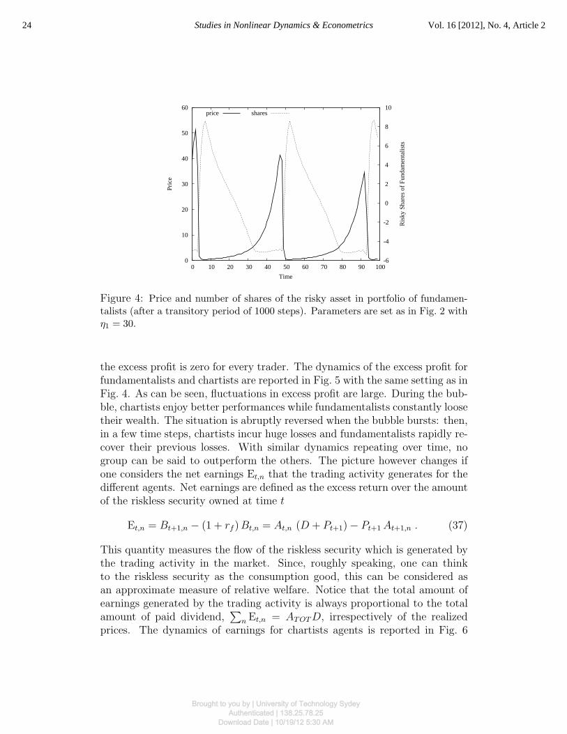
ferent groups of agents. Consider for instance the amount of risky shares At

owned by fundamentalists at time t. This is reported in Fig. 4 together withthe price levels. The total amount of shares per trader is A = 2. Negativeshares correspond to short positions. Notice that in the period of increasingprices (for instance, steps 10 − 30), the amount of shares in fundamentalists’portfolio is initially decreasing. Since chartists are willing to buy the riskyasset, fundamentalists eventually reach short positions. On the contrary, thebursting of the speculative bubble corresponds to a reallocation of the riskyasset toward fundamentalists, who now are willing to take long positions in anasset they consider undervalued.

It is interesting to know if and to what extent the joint dynamics ofprices and portfolio composition is more valuable for one group of agents com-pared to the other. To investigate this issue consider the excess profit Πt,n

received by agent n at time t

Πt,n = Wt+1,n − (1 + rf )Wt,n = At,n (Pt+1 +D − Pt(1 + rf )) . (36)

This quantity depends on both the dividend payment and the relative appre-ciation (or depreciation) of the risky asset. Notice that at equilibrium Pt = P ,




0

10

20

30

40

50

60

0 10 20 30 40 50 60 70 80 90 100-6

-4

-2

0

2

4

6

8

10

Pric

e

Ris

ky S

hare

s of

Fun

dam

enta

lists

Time

price shares

Figure 4: Price and number of shares of the risky asset in portfolio of fundamen-talists (after a transitory period of 1000 steps). Parameters are set as in Fig. 2 withη1 = 30.

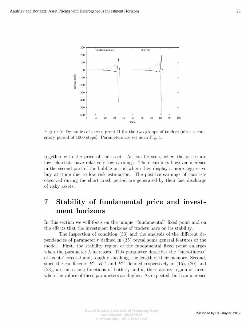
the excess profit is zero for every trader. The dynamics of the excess profit forfundamentalists and chartists are reported in Fig. 5 with the same setting as inFig. 4. As can be seen, fluctuations in excess profit are large. During the bub-ble, chartists enjoy better performances while fundamentalists constantly loosetheir wealth. The situation is abruptly reversed when the bubble bursts: then,in a few time steps, chartists incur huge losses and fundamentalists rapidly re-cover their previous losses. With similar dynamics repeating over time, nogroup can be said to outperform the others. The picture however changes ifone considers the net earnings Et,n that the trading activity generates for thedifferent agents. Net earnings are defined as the excess return over the amountof the riskless security owned at time t

Et,n = Bt+1,n − (1 + rf )Bt,n = At,n (D + Pt+1)− Pt+1 At+1,n . (37)

This quantity measures the flow of the riskless security which is generated bythe trading activity in the market. Since, roughly speaking, one can thinkto the riskless security as the consumption good, this can be considered asan approximate measure of relative welfare. Notice that the total amount ofearnings generated by the trading activity is always proportional to the totalamount of paid dividend,

∑n Et,n = ATOTD, irrespectively of the realized

prices. The dynamics of earnings for chartists agents is reported in Fig. 6




-600

-500

-400

-300

-200

-100

0

100

200

300

0 10 20 30 40 50 60 70 80 90 100

Exc

ess

Prof

it

Time

fundamentalists chartists

Figure 5: Dynamics of excess profit Π for the two groups of traders (after a tran-sitory period of 1000 steps). Parameters are set as in Fig. 4.

together with the price of the asset. As can be seen, when the prices arelow, chartists have relatively low earnings. Their earnings however increasein the second part of the bubble period where they display a more aggressivebuy attitude due to low risk estimation. The positive earnings of chartistsobserved during the short crash period are generated by their fast dischargeof risky assets.

7 Stability of fundamental price and invest-

ment horizons

In this section we will focus on the unique “fundamental” fixed point and onthe effects that the investment horizons of traders have on its stability.

The inspection of condition (33) and the analysis of the different de-pendencies of parameter r defined in (35) reveal some general features of themodel. First, the stability region of the fundamental fixed point enlargeswhen the parameter λ increases. This parameter describes the “smoothness”of agents’ forecast and, roughly speaking, the length of their memory. Second,since the coefficients BC, BUF and BSF defined respectively in (15), (20) and(23), are increasing functions of both rf and θ, the stability region is largerwhen the values of these parameters are higher. As expected, both an increase




-10

-5

0

5

10

15

0 10 20 30 40 50 60 70 80 90 100 0

5

10

15

20

25

30

35

40

45

50

Ear

ning

s of

cha

rtis

ts

Pric

e

Time

chart. earnings price

Figure 6: Dynamics of trading earnings E for the group of chartists compared withasset prices (after a transitory period of 1000 steps). Parameters are set as in Fig. 4.

in the riskless return and in the perceived efficiency of the market in restoringthe fundamental price tend to stabilize the dynamics. Third, since

BC(η) ≤ BUF(η, θ) and BC(η) ≤ BSF(η, θ) ∀η, ∀θ ,

an increase of the share of fundamentalists in the market will enlarge, ceterisparibus, the stability domain of the fixed point. These results are quite in-tuitive and do not require further comments. Their emergence can be tracedback to the assumptions about agents’ behavior and market structure.

Let us now turn to the analysis of the role of investment horizons.Notice that the only effect of the investment horizons on the stability of thesystem is through the definition of the parameter r which appears in (33). Moreprecisely, the investment horizons of the different group of agents contribute tothe definition of r via the coefficients BC, BUF and BSF defined in Section 3.3.

First of all, we observe that when a single type of agents is presentalone in market, would it be fundamentalist or chartist, an increase of thetime horizon does not disturb the stability of the system. As already discussedin Section 4, when only fundamentalists are present in the market, the fixedpoint is always stable. Concerning the chartists, if one considers (31) and setsf1 = 0, the parameter r only depends on term BC(η2). Since

dBC(η)

dη=

(1 + rf )η (η ln(1 + rf )− 1) + 1

η> 0 ∀η ≥ 1 .




0.01

0.1

1

10

100

10 20 30 40 50 60 70 80 90 100

dem

and

η

coefficient BC

coefficient BUF

coefficient BSF

Figure 7: Behavior of coefficients BC, BUF and BSF as functions of η for θ = 0.4and rf = 0.05.

this term is increasing function of η2. Thus, also in the case of chartists, anincrease of the investment horizon enlarges the stability domain of the fixedpoint.

The last result can be immediately extended to the case in which bothtypes are present in the market. Indeed the parameter r in (35) is an increasingfunction of ηc. Consequently, an increase of chartists’ horizon always stabilizesthe market, see illustration in Fig. 7, where the η-dependent factors of thedifferent demand functions are shown.

The same conclusion, however, does not apply to the investment hori-zon of unsophisticated fundamentalists. Consider the case in which the marketis populated by a group of chartists and a group of unsophisticated fundamen-talists, described in Section 5.1. Figure 8 is a bifurcation diagram of price: wecompute the set of price spanned by the system for different values of η1, theparameter describing the time horizon of fundamentalists. As one can see, forsmall values of η1, the dynamics stabilize around the fixed point. When η1increases, the system looses stability and goes to the region where dynamicsis similar to Fig. 2. Hence, in the presence of two types of agents, the increaseof the investment horizon of unsophisticated fundamentalists can have a detri-mental effect on the stability of the fixed point. However, when η1 increasesfurther the fundamental value becomes stable again.

This result comes quite unexpected. Indeed, almost by definition, the




0.1

1

10

100

0 10 20 30 40 50 60 70 80

Pric

e

Horizon of Fundamentalists, η1

Figure 8: Bifurcation diagram. The price support of a 1000 steps orbit (after a1000 steps transient) is shown in the log-scale for different values of η1 from 1 to80. The values of the other parameters and the initial conditions are the same as inFig. 2.

behavior of the fundamentalist traders, who buy the asset when its price isbelow the fundamental level and sell it when the price is above the fundamen-tal, should bring stability to the system. The explanation has to be searchedin the dependence of the fundamentalists’ demand function (19) on the in-vestment horizon captured by the coefficient BUF defined in (20). Indeed, itturns out that this coefficient is a non-monotonic function of the investmenthorizon η. In Fig. 9 we report the increments in the value of BUF when ηincreases from 1 to 2, 2 to 3, and 3 to 4, as a function of parameters rf andθ. For large values of θ and small values of rf these increments are negative,meaning that the optimal portfolio on longer time horizons contains a loweramount of risky security. However, we also observe that with increase of η,the region where BUF (η+1, θ) < BUF (η, θ) shrinks, so that, eventually, BUF

becomes an increasing function of η for any values of θ > 0 and rf , see alsoFig. 7. Even if the increase of horizons will eventually drive the system in theregion of stability, for small enough values of η1, an increase of the horizon offundamentalists can break the stability of the fixed point, while an increase ofthe horizon of chartists can not.

Finally, since coefficient BSF is an increasing function of η for any valueof θ and rf , an increase of the time horizons of the sophisticated fundamen-




η=1η=2η=3

0 0.2 0.4 0.6 0.8 1rf 0

0.2 0.4

0.6 0.8

1

θ

-0.4-0.2

0 0.2 0.4 0.6 0.8

Figure 9: First difference BUF(η + 1, θ) − BUF(η, θ) as a function of rf and θ fordifferent values of η. The intersections of the surfaces with the z = 0 plane areshown at the bottom of the graph.

talists always enlarges the stability domain of the “fundamental” fixed point,see Fig. 7.

The destabilizing effect of an increase of the unsophisticated fundamen-talists’ investment horizons observed in model with mixed population can beexplained as a substitution effect of the demand structure. Indeed, the non-linear pricing equation (9) is defined in terms of the weighted demand of thedifferent groups of traders. The stability/instability of the dynamics depends,therefore, not only on the total demand but also on the relative influenceof fundamentalists (which contribute to the stabilization of the system) andchartists (who create the opposite effect). When the investment horizon of theunsophisticated fundamentalists increases (and not large enough), their totaldemand all other parameters being equal will decrease, as it is seen from Fig. 7.The overall effect is then equivalent to a reduction of the number of fundamen-talists in the market: in this case the substitution effect plays a destabilizingrole. On the other hand, if the fundamentalists form the long-term forecast forthe variance according to (21), which increases with η1 slower than (18), thenthe substitution effect plays a stabilizing role, increasing the relative weight ofthe fundamentalist traders in the market.




8 Conclusions

This paper extends the asset pricing model introduced in Bottazzi (2002) to in-corporate heterogeneity in traders’ investment horizons. Traders are describedas mean-variance utility maximizers. They have different expectations aboutfuture returns and plan their investments over different time horizons.

Our first result is that the sole heterogeneity of investment horizons isnot enough to destabilize the dynamics of prices. In other words, the marketbehavior is affected by the investment horizons of agents only when they pos-sess heterogeneous beliefs about future prices. This result is relevant for thesearch of the minimal heterogeneity requirements sufficient to explain observedempirical regularity, e.g., excess volatility.

When a mixed populations of traders is considered, one observes theemergence of non-obvious effects of the length of the investment horizons on themarket price. Indeed, we found that minor changes in the investment horizonsof some sub-population of agents may lead to large qualitative changes in thedynamics of price. In general, however, the strength and nature with which avariation in investment horizons affects the market dynamics strongly dependon the ecology of agents considered. The overall effect can be traced back tothe different behavior of agents individual demand functions when investmentof different maturities are considered. These differences come, in turn, fromthe way in which different agents estimate long-run risk.

One obvious limit of the previous investigation resides in the simplify-ing assumption of a Walrasian market clearing. Indeed, it would be interestingto investigate our behavioral model in a different, non Walrasian, market ar-chitecture. As shown by Bottazzi et al. (2005) and Anufriev and Panchenko(2009) the trading protocol can have a big impact on the dynamics of price.For instance, LiCalzi and Pellizzari (2003) simulate an order-driven stock mar-ket which is operated through the book of orders. In their model all agentsare fundamentalists and only differ with respect to their investment horizons.Nevertheless, they are able to generate time series with properties similar tothe ones observed in real markets.

A second interesting extension would be the introduction of an endoge-nous mechanism in the selection of investment horizons. One possibility is touse the framework presented in Brock and Hommes (1998) and root the choiceof the horizon inside the random utility theory. This extension could poten-tially enrich our model, in which horizons are exogenously given and fixed,and lead to an extension of the model in Osler (1995) where the dynamicalaspect of the endogenous choice of horizons is absent.




APPENDIX

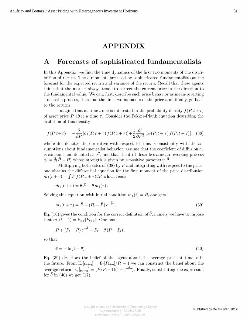
A Forecasts of sophisticated fundamentalists

In this Appendix, we find the time dynamics of the first two moments of the distri-bution of return. These moments are used by sophisticated fundamentalists as theforecast for the expected return and variance of the return. Recall that these agentsthink that the market always tends to correct the current price in the direction tothe fundamental value. We can, first, describe such price behavior as mean-revertingstochastic process, then find the first two moments of the price and, finally, go backto the returns.

Imagine that at time t one is interested in the probability density f(P, t+ τ)of asset price P after a time τ . Consider the Fokker-Plank equation describing theevolution of this density

f(P, t+τ) = − ∂

∂P[a1(P, t+ τ) f(P, t+ τ)]+

1

2

∂2

∂P 2[a2(P, t+ τ) f(P, t+ τ)] , (38)

where dot denotes the derivative with respect to time. Consistently with the as-sumptions about fundamentalist behavior, assume that the coefficient of diffusion a2is constant and denoted as σ2, and that the drift describes a mean reversing processa1 = θ(P − P ) whose strength is given by a positive parameter θ.

Multiplying both sides of (38) by P and integrating with respect to the price,one obtains the differential equation for the first moment of the price distributionm1(t+ τ) =

∫P f(P, t+ τ)dP which reads

m1(t+ τ) = θ P − θ m1(τ) .

Solving this equation with initial condition m1(t) = Pt one gets

m1(t+ τ) = P + (Pt − P ) e−θτ . (39)

Eq. (16) gives the condition for the correct definition of θ, namely we have to imposethat m1(t+ 1) = Et,f [Pt+1]. One has

P + (Pt − P ) e−θ = Pt + θ (P − Pt) ,

so that

θ = − ln(1− θ) . (40)

Eq. (39) describes the belief of the agent about the average price at time τ inthe future. From Et[ρt+η] = Et[Pt+η]/Pt − 1 we can construct the belief about the

average return: Et[ρt+η] = (P /Pt−1)(1−e−θη). Finally, substituting the expressionfor θ in (40) we get (17).




A similar procedure is repeated for the second moment. Multiplying bothsides of (38) by P 2 and integrating with respect to P , one gets the differentialequation for the second moment of price m2(t + τ) =

∫P 2 f(P, t + τ) dP which

reads

m2(t+ τ) = σ2 + 2θ P m1(t+ τ)− 2 θ m2(t+ τ) .

The solution with initial condition m2(t) = P 2t becomes

m2(t+ τ) =σ2

2 θ+ P 2+2P (Pt− P )e−θτ +

(P 2t − σ2

2 θ− P 2− 2 P (Pt− P )

)e−2θτ .

Now using the expression for the first two moments of the price distribution, we cancompute the belief of the fundamentalists about the variance Vt,f [ρt,t+η],

Vt,f [ρt,t+η] =1

P 2t

(m2(t+ η)−m1(t+ η)2

)=

σ2

2θP 2t

(1− e−2θη

).

To get rid of the parameter σ2 we assume that the one period ahead forecastof fundamentalists coincides with the forecast of chartists, i.e., it is given by theEWMA estimator zt−1. Then

σ2 =2θP 2

t

1− e−2θzt−1 ,

and, finally,

Vt,f [ρt,t+η] =1− e−2θη

1− e−2θzt−1 .

Substituting the expression for θ in (40) one gets (21).Finally notice that the chartists forecasting rules (12) and (13) can be ob-

tained following the same procedure but assuming constant drift and variance inthe Fokker-Plank equation (38).

B Proof of Proposition (4.1)

First of all notice that even if the function f in (27) is defined for positive arguments,it can be extended continuously to z = 0. In fact

limz→0

f(z) =s

r= γP .

Thus, system (27) is defined for any y and for z ≥ 0.In order to find the possible fixed points of the system assume that Pt+1 =

Pt = P ∗. Using the second equation, this implies that yt+1 = λyt. If λ > 0, the




condition yt+1 = yt implies yt = 0. The same applies to the equation for zt. Then,substituting yt = zt = 0 in the first equation, one concludes that the system hasonly the fixed point (γP , 0, 0), which corresponds to the fundamental price with zeroforecasted variance.

The local stability of the point can be checked computing the Jacobian ma-trix. First, note that the derivative of function f reads

f ′(z) =1

z

(s√

r2 + 4sz− f(z)

).

This derivative can be extended to the point z = 0 continuously, and one hasf ′(0) = −s2/r3. Consequently the Jacobian matrix in (γP , 0, 0) reads

J(p, y, z)(γP ,0,0)

=

∥∥∥∥∥∥∥∥0 0 f ′(0)

−(1− λ) f(0)(γP )2

λ (1− λ)f′(0)γP

−2λ(1− λ) f(0)(γP )2

h −2λ(1− λ)h λ+ 2λ(1− λ)hf ′(0)(γP )

∥∥∥∥∥∥∥∥ ,

where h stands for the value of the function h(p, y, z) = f(z)p − 1 − y in (γP , 0, 0).

Since h = 0, the Jacobian in the fixed point can be simplified to become

J(p, y, z)(γP ,0,0)

=

∥∥∥∥∥∥∥0 0 −s2/r3

−(1− λ)r/s λ −(1− λ)s/r2

0 0 0

∥∥∥∥∥∥∥ .

The eigenvalues of J(p, y, z) are λ and 0 (with multiplicity two), which implies thatthe point (γP , 0, 0) is locally asymptotically stable as far as 0 ≤ λ < 1.

References

Allen, H. and M. P. Taylor (1990): “Charts, noise and fundamentals in the londonforeign exchange market,” Economic Journal, 100, 49–59.

Anufriev, M. and G. Bottazzi (2010): “Market equilibria under procedural rational-ity,” Journal of Mathematical Economics, 46, 1140 – 1172.

Anufriev, M., G. Bottazzi, and F. Pancotto (2006): “Equilibria, stability and asymp-totic dominance in a speculative market with heterogeneous agents,” Journal ofEconomic Dynamics & Control, 30, 1787–1835.

Anufriev, M. and V. Panchenko (2009): “Asset prices, traders’ behavior and marketdesign,” Journal of Economic Dynamics & Control, 33, 1073 – 1090.




Arthur, W., J. H. Holland, B. LeBaron, R. Palmer, and P. Tayler (1997): “As-set pricing under endogenous expectations in an artificial stock market,” inW. Arthur, S. N. Durlauf, and D. A. Lane, eds., The Economy as an EvolvingComplex System II, Addison-Wesley, 15–44.

Bottazzi, G. (2002): “A simple micro-model of market dynamics. part i: the ”largemarket” deterministic limit,” LEM Working Paper 2002-10, Sant’Anna School forAdvanced Studies, Pisa.

Bottazzi, G., G. Dosi, and I. Rebesco (2005): “Institutional achitectures and be-havioural ecologies in the dynamics of financial markets: a preliminary investiga-tion,” Journal of Mathematical Economics, 41, 197–228.

Brock, W. A. (1997): “Asset price behavior in complex environment,” in W. Arthur,S. N. Durlauf, and D. A. Lane, eds., The Economy as an Evolving Complex SystemII, Addison-Wesley, 385–423.

Brock, W. A. and C. H. Hommes (1998): “Heterogeneous beliefs and routes to chaosin a simple asset pricing model,” Journal of Economic Dynamics & Control, 22,1235–1274.

Brock, W. A., C. H. Hommes, and F. O. Wagener (2005): “Evolutionary dynamicsin markets with many trader types,” Journal of Mathematical Economics, 41,7–42.

Brock, W. A. and B. LeBaron (1996): “A dynamic structural model for stock returnvolatility and trading volume,” Review of Economics and Statistics, 78, 94–110.

Campbell, J. Y. and L. M. Viceira (2002): Strategic Asset Allocation: PortfolioChoice for Long-Term Investors, Oxford University Press, Oxford.

Chiarella, C., R. Dieci, and L. Gardini (2006): “Asset price and wealth dynamics ina financial market with heterogeneous agents,” Journal of Economic Dynamics& Control, 30, 1755–1786.

Chiarella, C. and X.-Z. He (2001): “Asset price and wealth dynamics under hetero-geneous expectations,” Quantitative Finance, 1, 509–526.

Dacorogna, M. M., R. Gencay, U. A. Muller, R. B. Olsen, and O. V. Pictet (2001):An Introduction to High-Frequency Finance, Academic Press, New York.

Dacorogna, M. M., U. A. Muller, C. Jost, O. V. Pictet, R. B. Olsen, and J. R.Ward (1995): “Heterogeneous real-time trading strategies in the foreign exchangemarkets,” The European Journal of Finance, 1, 383–403.




Fama, E. F. (1970): “Efficient capital markets: a review of theory and empiricalwork,” Journal of Finance, 25, 383–422.

Frankel, J. A. and K. A. Froot (1987a): “Short-term and long-term expectationsof the yen/dollar exchange rate: Evidence from survey data,” Journal of theJapanese and International Economies, 1, 249–274.

Frankel, J. A. and K. A. Froot (1987b): “Using survey data to test standard propo-sitions regarding exchange rate expectations,” American Economic Review, 77,133–153.

Froot, K. A., D. S. Scharfstein, and J. C. Stein (1992): “Herd on the street: In-formational inefficiencies in a market with short-term speculation,” Journal ofFinance, 47, 1461–1484.

Gaunersdorfer, A. (2000): “Endogenous fluctuations in a simple asset pricing modelwith heterogeneous agents,” Journal of Economic Dynamics & Control, 24, 799–831.

Guillaume, D. M., M. M. Dacorogna, R. R. Dave, U. A. Muller, R. B. Olsen, andO. V. Pictet (1997): “From the bird’s eye to the microscope: A survey of new styl-ized facts of the intra-daily foreign exchange markets,” Finance and Stochastics,1, 95–129.

Hillebrand, M. and J. Wenzelburger (2006): “The impact of multiperiod planninghorizons on portfolios and asset prices in a dynamic capm,” Journal of Mathe-matical Economics, 42, 565–593.

Hommes, C. H. (2006): “Heterogeneous agent models in economics and finance,”in K. L. Judd and L. Tesfatsion, eds., Handbook of Computational EconomicsVol. 2: Agent-Based Computational Economics, North-Holland (Handbooks inEconomics Series), Amsterdam.

Ito, T. (1990): “Foreign exchange rate expectations: Micro survey data,” AmericanEconomic Review, 80, 434–449.

J.P.Morgan (1996): RiskMetricsTM– Technical Document, Morgan Guaranty TrustCompany of New York, New York, 4 edition.

Kirman, A. (2006): “Heterogeneity in economics,” Journal of Economic Interactionand Coordination, 1, 89–117.

Kirman, A. and G. Teyssiere (2002): “Bubbles and long range dependence in assetprices volatilities,” in H. C. H., R. Ramer, and C. Withagen, eds., Equilibrium,Markets and Dynamics, Springer, 307–328.




LeBaron, B. (2006): “Agent-based computational finance,” in K. L. Judd and L. Tes-fatsion, eds., Handbook of Computational Economics Vol. 2: Agent-Based Com-putational Economics, North-Holland (Handbooks in Economics Series).

LeRoy, S. F. (1973): “Risk aversion and the martingale property of stock prices,”International Economics Review, 14, 436–446.

Levy, M., H. Levy, and S. Solomon (1994): “A microscopic model of the stockmarket: Cycles, booms, and crashes,” Economics Letters, 45, 103–111.

LiCalzi, M. and P. Pellizzari (2003): “Fundamentalists clashing over the book: astudy of order-driven stock markets,” Quantitative Finance, 3, 1–11.

Lucas, R. E. (1978): “Asset prices in an exchange economy,” Econometrica, 46,1429–1445.

Lux, T. (1995): “Herd behaviour, bubbles and crashes,” The Economic Journal,105, 881–896.

Lux, T. and M. Marchesi (1999): “Scaling and criticality in a stochastic multi-agentmodel of financial market,” Nature, 397, 498–500.

Manzan, S. and F. Westerhoff (2007): “Heterogeneous expectations, exchange ratedynamics and predictability,” Journal of Economic Behavior & Organization, 64,111–128.

Merton, R. C. (1973): “An intertemporal capital asset pricing model,” Economet-rica, 41, 867–887.

Osler, C. L. (1995): “Exchange rate dynamics and speculator horizons,” Journal ofInternational Money and Finance, 14, 695–719.

Samuelson, P. A. (1969): “Lifetime portfolio selection by dynamic stochastic pro-gramming,” Review of Economics and Statistics, 51, 239–246.

Westerhoff, F. and S. Reitz (2003): “Nonlinearities and cyclical behavior: the role ofchartists and fundamentalists,” Studies in Nonlinear Dynamics & Econometrics,7, 1–12.




studies in nonlinear dynamics &...

Documents