Studies of Optimal Track-Fitting Techniques for

the DarkLight Experiment

by

Purnima Parvathy Balakrishnan

Submitted to the Department of Physicsin partial fulfillment of the requirements for the degree of

Bachelor of Science

at the

MASSACHUSETTS INSTITUTE OF TECHNOLOGY

June 2013

INSTIThTE0 TECR 'OLOGY

SEP 0 4 2013

2 RARIES

@ Purnima Parvathy Balakrishnan, MMXIII. All rights reserved.

The author hereby grants to MIT permission to reproduce and todistribute publicly paper and electronic copies of this thesis document

in whole or in part in any medium now known or hereafter created.

A uthor .............................................Department of Physics

.4 ' May 17, 2013

Certified by....................... .. ..................Peter Fisher

ProfessorThesis Supervisor, Department of Physics

A ccepted by .................. ............Professor Nergis Mavalvala

Senior Thesis Coordinator, Department of Physics

2

Studies of Optimal Track-Fitting Techniques for the

DarkLight Experiment

by

Purnima Parvathy Balakrishnan

Submitted to the Department of Physics

on May 17, 2013, in partial fulfillment of the

requirements for the degree of

Bachelor of Science

Abstract

The DarkLight experiment is searching for a dark force carrier, the A' boson, and

hopes to measure its mass with a resolution of approximately 1 MeV/c 2 . This mass

calculation requires precise reconstruction to turn data, in the form of hits within the

detector, into a particle track with known initial momentum. This thesis investigates

the appropriateness of the Billoir optimal fit to reconstruct helical, low-energy lepton

tracks while accounting for multiple scattering, using two separate track parameter-

izations. The first method approximates the track as a piecewise concatenation of

parabolas in three-dimensions, and (wrongly) assumes that the y and z components

of the track are independent. When tested using simulated data, this returns a track

which geometrically fits the data. However, the momentum extracted from this geo-

metrical representation is an order of magnitude higher than the true momentum of

the track. The second method approximates the track as a piecewise concatenation

of helical segments. This returns a track which geometrically fits the data even better

than the parabolic parameterization, but which returns a momentum which depends

on the seeds to the algorithm. Some further work must be done to modify this fitting

method so that it will reliably reconstruct tracks.

Thesis Supervisor: Peter Fisher

Title: Professor

3

4

Acknowledgments

I would like to thank Peter Fisher and Ray Cowan for all of their help and support

on this project.

5

6

Contents

1 Introduction 13

1.1 Dark Matter and DarkLight . . . . . . . . . . . . . . . . . . . . . . . 13

1.2 Tracking Chambers . . . . . . . . . . . . . . . . . . . . . . . . . . . . 14

1.3 Track Reconstruction . . . . . . . . . . . . . . . . . . . . . . . . . . . 15

2 Prior Work 17

2.1 Geant4 Detector Simulation . . . . . . . . . . . . . . . . . . . . . . . 18

2.2 Karimiki Circle Fit . . . . . . . . . . . . . . . . . . . . . . . . . . . . 19

3 Problem Statement 21

3.1 Multiple Scattering . . . . . . . . . . . . . . . . . . . . . . . . . . . . 21

3.2 Karimdki Fit Problems . . . . . . . . . . . . . . . . . . . . . . . . . . 22

4 Separable Billoir Fit 25

4.1 Billoir Recursive Method . . . . . . . . . . . . . . . . . . . . . . . . . 25

4.2 Separable Track Parameterization . . . . . . . . . . . . . . . . . . . . 27

4.2.1 Matrices for the Billoir Method . . . . . . . . . . . . . . . . . 28

4.3 Implementation . . . . . . . . . . . . . . . . . . . . . . . . . . . . . . 29

4.3.1 Parameter Seeding . . . . . . . . . . . . . . . . . . . . . . . . 30

4.3.2 Error Seeding . . . . . . . . . . . . . . . . . . . . . . . . . . . 30

4.3.3 Iteration . . . . . . . . . . . . . . . . . . . . . . . . . . . . . . 32

5 Results of separable fit 33

5.1 Position . . . . . . . . . . . . . . . . . . . . . . . . . . . . . . . . . . 33

7

5.2 M omentum ................................ 33

5.3 Conclusions . . . . . . . . . . . . . . . . . . . . . . . . . . . . . . . . 35

6 Helical 5-Parameter Fit 37

6.1 Helical Parameterization ......................... 37

6.2 Implementation .............................. 39

7 Results of 5-parameter fit 41

7.1 Position . . . . . . . . . . . . . . . . . . . . . . . . . . . . . . . . . . 41

7.2 M omentum . . . . . . . . . . . . . . . . . . . . . . . . . . . . . . . . 41

7.3 Propagation of Parameters to Origin . . . . . . . . . . . . . . . . . . 43

8 Summary, Conclusions, and Future Work 45

8.1 Billoir M ethod . . . . . . . . . . . . . . . . . . . . . . . . . . . . . . . 46

8.1.1 Separable Fit . . . . . . . . . . . . . . . . . . . . . . . . . . . 46

8.1.2 Helical Fit . . . . . . . . . . . . . . . . . . . . . . . . . . . . . 46

8.2 Future W ork . . . . . . . . . . . . . . . . . . . . . . . . . . . . . . . . 47

8.2.1 Fixing the Billoir Helical Fit . . . . . . . . . . . . . . . . . . . 47

8.2.2 Testing and Using the Billoir Helical Fit . . . . . . . . . . . . 48

8

List of Figures

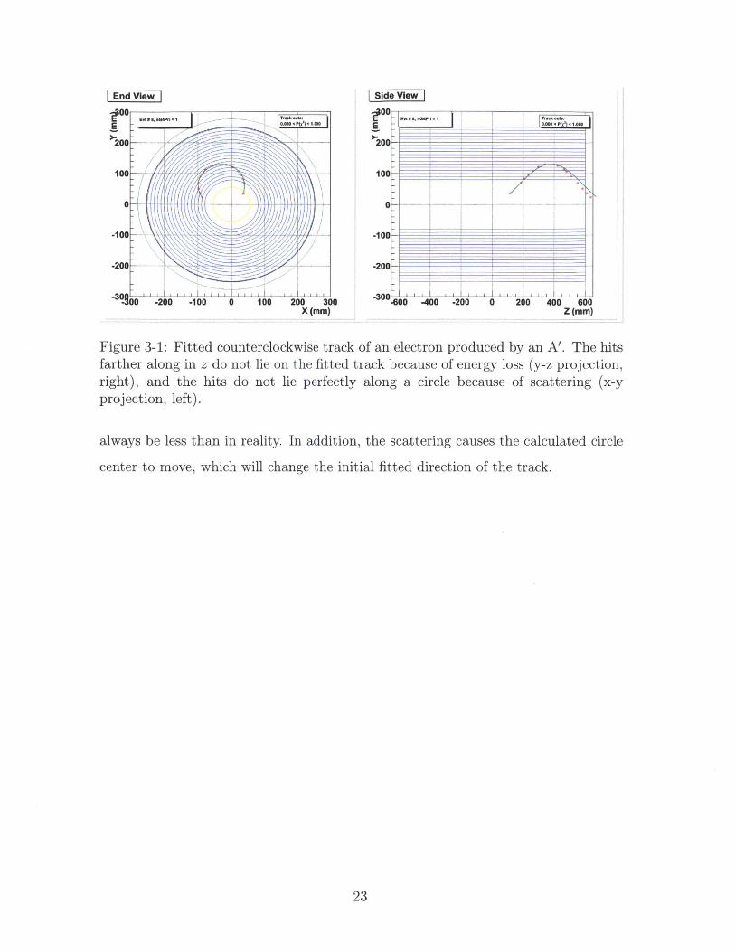
3-1 Fitted counterclockwise track of an electron produced by an A'. The

hits farther along in z do not lie on the fitted track because of energy

loss (y-z projection, right), and the hits do not lie perfectly along a

circle because of scattering (x-y projection, left). . . . . . . . . . . . . 23

5-1 Comparison of measured and parabolically fitted y-coordinates. Dis-

crepancy between the two is approximately 2 mm at each point. The

crosses are for easier viewing of the data, not error bars. . . . . . . . 34

5-2 Comparison of measured and linearly fitted z-coordinates. Discrepancy

between the two is approximately 1.5 mm at each point. . . . . . . . 34

6-1 The 5 parameters of a helix are the radius R, dip angle A, azimuthal

angle 0 (related to the phase), y and z [2]. Note that the center

of the helix is a line parallel to the z-axis, but not necessarily going

through the origin. 0 and y contain the same information as the center

coordinates xO and yo. . . . . . . . . . . . . . . . . . . . . . . . . . . 37

7-1 Comparison of measured and helically fitted y-coordinates. Discrep-

ancy between the two is approximately .02 mm at each point. .... 42

7-2 Comparison of measured and helically fitted z-coordinates. Discrep-

ancy between the two is approximately .01 mm at each point. .... 42

9

10

List of Tables

5.1 Dependence of momentum, calculated from separable fit, on initial

parameter error. . . . . . . . . . . . . . . . . . . . . . . . . . . . . . . 35

7.1 Dependence of momentum, calculated from helix fit, on initial param-

eter error. ....... ......... . . ................... 43

7.2 Dependence of calculated "initial" position and momentum on initial

parameter errors. . . . . . . . . . . . . . . . . . . . . . . . . . . . . . 44

11

12

Chapter 1

Introduction

Track reconstruction is essential for analyzing data produced by tracking particle

detectors. While they are ubiquitous, different experiments require different types of

track-fitting methods.

This chapter will describe the motivations behind the DarkLight experiment and

the need for an accurate particle track reconstruction algorithm. Chapter two will

cover prior work done in simulating and fitting these tracks. Chapter three will

describe the problems with current track-fitting solutions, and requirements for a more

appropriate one for this experiment. Chapters four and six will cover two different

approaches to this problem, while chapters five and seven will cover their respective

results. Lastly chapter eight contains conclusions and a discussion of possible future

work.

1.1 Dark Matter and DarkLight

There is significant evidence that the universe contains what is called dark matter:

matter that we have not yet observed because it does not interact electromagneti-

cally, but is around in large enough quantities that we can detect its cosmological

effects. There are currently many theories for what dark matter consists of - axions,

weakly interacting massive particles (WIMPS), neutrinos, supersymmetric particles,

and more - and many more experiments searching for them, either directly or in-

13

directly. New theories, motivated in part by evidence for the excess production of

electron/positron pairs in our galaxy, predict a dark force, mediated by a neutral

light (low-mass) particle, called the A' boson. The A' is produced in dark matter

interactions, but also decays via electron/positron pair production [4].

The DarkLight experiment (Detecting A Resonance Kinematically with eLectrons

Incident on a Gaseous Hydrogen Target) is currently being developed to create and

observe this new boson through the following process:

e +p -+ e-+p + e-+ (1 1)

DarkLight will be run using the Jefferson Lab Free Electron Laser (FEL), using a

1 MW, 100 MeV electron beam incident on a gaseous hydrogen (proton) target. This

collision will cause pair production through electromagnetic processes, which are the

most significant source of background, but should also pair produce through A'. An

excess of electrons and positrons at a specific total energy would allow us to determine

the mass mAI of the particle and coupling strength a' of the corresponding force.

DarkLight is designed to detect A' in the mass range of 10-100 MeV and coupling

strength range of 10-9-10-7.

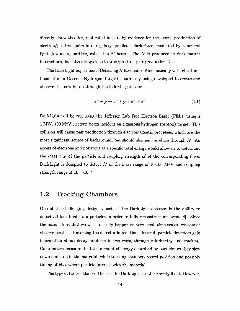
1.2 Tracking Chambers

One of the challenging design aspects of the DarkLight detector is the ability to

detect all four final-state particles in order to fully reconstruct an event [4]. Since

the interactions that we wish to study happen on very small time scales, we cannot

observe particles traversing the detector in real-time. Instead, particle detectors gain

information about decay products in two ways, through calorimetry and tracking.

Calorimeters measure the total amount of energy deposited by particles as they slow

down and stop in the material, while tracking chambers record position and possibly

timing of hits, where particle interact with the material.

The type of tracker that will be used for DarkLight is not currently fixed. However,

14

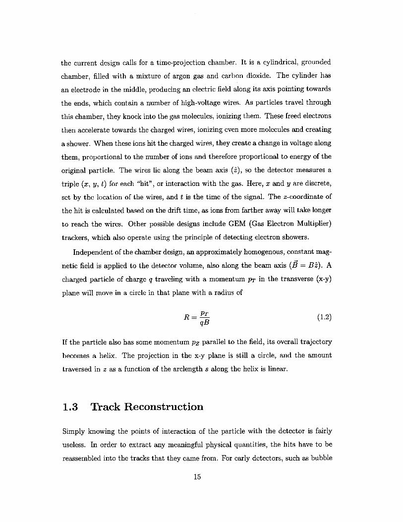
the current design calls for a time-projection chamber. It is a cylindrical, grounded

chamber, filled with a mixture of argon gas and carbon dioxide. The cylinder has

an electrode in the middle, producing an electric field along its axis pointing towards

the ends, which contain a number of high-voltage wires. As particles travel through

this chamber, they knock into the gas molecules, ionizing them. These freed electrons

then accelerate towards the charged wires, ionizing even more molecules and creating

a shower. When these ions hit the charged wires, they create a change in voltage along

them, proportional to the number of ions and therefore proportional to energy of the

original particle. The wires lie along the beam axis (i), so the detector measures a

triple (x, y, t) for each "hit", or interaction with the gas. Here, x and y are discrete,

set by the location of the wires, and t is the time of the signal. The z-coordinate of

the hit is calculated based on the drift time, as ions from farther away will take longer

to reach the wires. Other possible designs include GEM (Gas Electron Multiplier)

trackers, which also operate using the principle of detecting electron showers.

Independent of the chamber design, an approximately homogenous, constant mag-

netic field is applied to the detector volume, also along the beam axis (B = B ). A

charged particle of charge q traveling with a momentum p' in the transverse (x-y)

plane will move in a circle in that plane with a radius of

R= T (1.2)qB

If the particle also has some momentum pz parallel to the field, its overall trajectory

becomes a helix. The projection in the x-y plane is still a circle, and the amount

traversed in z as a function of the arclength s along the helix is linear.

1.3 Track Reconstruction

Simply knowing the points of interaction of the particle with the detector is fairly

useless. In order to extract any meaningful physical quantities, the hits have to be

reassembled into the tracks that they came from. For early detectors, such as bubble

15

chambers, which detect single tracks continuously, this task was done geometrically

by hand. For more complex experiments, where data is recorded digitally and hits

are sparser, this becomes more complicated.

First, when there are multiple tracks which overlap each other, the hits need to be

separated out and grouped based on which particle they originated from. Assuming

that this can be done, the hits can be fit by a continuous track, in order to determine

particle type, initial momentum, and initial position.

Using the initial momentum and masses of all four final-state particles (two elec-

trons, one positron, and one proton), we can calculate the center of mass energy of

the particle that created it, whether that be a photon or an A'. After many events

(of the interaction described in equation 1.1), there should be a slight excess of events

with invariant mass mA,. The coupling strength can be extracted by comparing this

excess (the signal) to the number of background events (electromagnetic noise).

The precision, or resolution of these measurements depend on the error of mea-

sured momentum, which in turn depends on the errors in the fitting algorithm. It

also depends on the detector's resolution in position and energy, which depends on

design and material properties. A more precise fitting algorithm allows more leeway

in the design of the detector.

The goal of my thesis was to write a track-fitting program that could be used to

evaluate and optimize detector design in order to have the mass resolution required

for the experiment. Finalization of the detector design is necessary in order to secure

funding, and in order to start physically building and testing detector components.

16

Chapter 2

Prior Work

Tracking algorithms are ubiquitous in particle physics experiments. They are ex-

tremely important for extracting any information from the huge number of hits that

are generated in any accelerator-based particle detector. However, there are many

problems with tracking algorithms that make them very difficult to reuse.

First and foremost, all tracking programs are either specific to or optimized for

the detector geometry of the experiment they are written for. This means that they

are written for specific shapes of trajectories (helices vs. lines), specific types of

detectors (wire chambers vs. spark chambers), or specific detector materials (argon

vs. helium), and are difficult, if not impossible, to generalize to other experiments.

In addition, different experiments have different requirements; one experiment may

need a very fast but rudimentary algorithm for discarding unneeded data (triggering),

while another may need a very accurate fit but have no time constraints.

Even if existing code is appropriate for reuse, it can be very difficult to adapt.

My first attempt to create a track-fitter was trying to adapt the Kalman Filter

from the Mu2e collaboration, which was originally written for the BaBar experi-

ment. During this attempt, I found that the Mu2e code was so dependent on other

collaboration-specific software - the uncommon build system, statistical libraries,

modeling libraries, and more - that the optimizations and accuracy guaranteed by

reusing their software was not worth the very long time that it would take to untan-

gle it and adapt it to our group's needs. For this reason, it was necessary to write a

17

track fitter from scratch, one that can be used to extract physical parameters of the

particle using information about the detector, and not just a geometric description

of the track.

2.1 Geant4 Detector Simulation

In order to test any track-fitters, there has to be a track with known parameters.

These tracks were generated by a simulation of the detector.

I wrote the simulation in C++ using ROOT (a statistical analysis framework) and

Geant4 (a particle simulation toolkit). The simulation takes particles and moves them

through the detector, simulating the interactions with the materials in the detector.

Depending on the interaction, the particle can deposit energy in the detector. This

is recorded as a hit, and the position (X, y, z), energy deposited dE, and volume

(tracking chamber vs. calorimeter) are recorded. These positions are exact, up to

truncation, because they are the positions of interaction within the gas, not of the

hit along the chamber wires.

The simulation can be seeded in two ways. First, a particle can be shot out of a

"particle gun", meaning that the event simply contains a particle with a given initial

position and momentum. Alternatively, the simulation can read in input from Mad-

Graph, which is a program which numerically calculates cross-sections of different

processes given their Feynman diagrams, and also generates events. It can produce

possible initial momenta for the final-state particles produced either by photons of

various energy (background) or by A' of a specific mass (signal). An accurate track-

fitter should be able to fit a track produced by the particle gun and calculate an

accurate initial momentum. It should then be able to fit tracks produced by Mad-

Graph and use the fitted momenta to calculate an accurate center-of-mass energy for

the event.

The simulation outputs "events", which contain all of the tracks produced by a

single interaction. Each track contains information about the initial position and

momentum, as well as a vector of hits. Each hit includes the coordinates (x, y, z),

18

deposited energy dE, and what part of the detector those coordinates lie in (e.g.

tracker, scintillator, beam dump, etc.). In reality, only a portion of this information

can be detected; the other (such as initial momentum) must be calculated from the

data. However, this allows us to test the track-fitters.

The type of hits generated by the simulation depend on the specific geometry of

the detector. Because the detector design is so fluid, the simulation has been modified

by other members of the group to be able to read in geometry from an XML file. This

allows things like the magnetic field strength, inner and outer radii of the tracker,

or gas concentration, to be easily changed and compared. A good track-fitter will

be able to give concrete values for the errors associated with track parameters for

different geometries.

2.2 Karimiki Circle Fit

A preliminary track fitter was written by Ray Cowan in ROOT. It fits tracks in two

consecutive steps. First, it takes the projection of the hits in the x-y plane and fits

the hits to a circle. It then calculates the arclength s for each point and fits the s-z

projection to a line.

The circular x-y fit is implemented using the Karimiki fit. This fit performs a

least-squares minimization in x and y to return the radius R and center point (X0 , Yo)

of the circle that best fits the points [6]. There is no order to the points, so all points

are equally weighted.

The second step is to use the circular fit parameters to calculate the arclength s

along the circular projection at each point. A standard linear least-squares regression

is performed to fit z linearly to s.

19

20

Chapter 3

Problem Statement

Although the Karimaki circe fitter does a decent job of getting good estimates for

initial momentum, it is not very precise. This is because the technique does not

take into account a very important physical process that occurs in particle detectors:

multiple scattering.

3.1 Multiple Scattering

As a high-energy (E > 10 MeV) electron (or positron) moves through a medium,

it interacts electromagnetically. Coulomb repulsion with atomic electrons causes the

particle to scatter, ionizing the atoms. It is this interaction that allows the detector

to function, but it also changes the particle trajectory. First, the particle scatters,

and second, the particle loses the energy required for ionization. This changes both

the direction and magnitude of the momentum, and changes the expected smooth

helical trajectory to one that has kinks (from scattering) and spirals inward (from

energy loss).

The amount of scattering that occurs is characterized by a property of the material

called the radiation length, X 0 . The energy of a particle that has travelled a single

radiation length drops to 1/e of its initial value. A particle with initial energy E0 ,

after traveling a distance x through a material, has an energy E = Eoe--/xO.

Radiation lengths for different materials are well known. For a mixture, the radi-

21

ation length is given by1 = i (3.1)

XOmix . .Xo,3 in mix

where wj is the fraction by weight of component j [5]. The current iteration of the

DarkLight tracker is filled with an 80:20 mixture of argon gas (Xo = 19.55g/cm2 ) and

carbon dioxide (XO = 36.20 g/cm2 ) [5] at a density of p = .0018 g/cm 3 ; this mixture

has a radiation length of 119.6 m. This is much larger than the length of the detector

(a single meter), so the energy loss is less significant than the direction change.

The scattering angle can be approximated as a Gaussian variable a with standard

deviation13.6 MeV

O = x/(I + .038 ln) (3.2)pv

where ( = is the number of radiation lengths of the material the particle has

passed through, p is the total momentum, and v is the total velocity [5]. Because the

electrons produced in the DarkLight experiment are much lower energy than those

produced in many high-energy experiments, they can scatter at much larger angles.

This makes an effect that is negligible at high energies very important, especially

because our goal is precision.

3.2 Karimfiki Fit Problems

This fitter was tested using both "particle gun" and MadGraph simulated data. Al-

though it does a good job at providing rough estimates of the particle momentum,

and fits the tracks fairly well, as shown in figure 3-1, the fit fails to be valid over the

entire track. This is due to not accounting for multiple scattering.

This discrepancy holds especially true for longer tracks, or ones that loop around

multiple times. Because they are in the tracker for longer, they scatter more and

the effects on the track become more significant. Loopers especially are not very

optimally fit using the Karimdki fitter, because as the electron stays in the tracker

longer, it spirals inward and creates multiple circles in the x-y projection. This causes

the overall calculated radius to decrease, and the calculated initial momentum will

22

End View S

200

0

-100

-200

-300 -200 -100 0

200

0

100 200 300X (mm)

Evt 8 8, .04Pi I10.0004 P(A~ - .000

--- ,

.~~~ .....

Figure 3-1: Fitted counterclockwise track of an electron produced by an A'. The hitsfarther along in z do not lie on the fitted track because of energy loss (y-z projection,right), and the hits do not lie perfectly along a circle because of scattering (x-yprojection, left).

always be less than in reality. In addition, the scattering causes the calculated circle

center to move, which will change the initial fitted direction of the track.

23

-100

-200

-300-'-600 -400 -200 0 200 400 600

z (mm)

24

Chapter 4

Separable Billoir Fit

In order to get an accurate reconstruction of the initial track momentum and position,

we require a method that takes into account multiple scattering. One such method

is Pierre Billoir's method for track fitting, developed in the 1980's for high-energy

physics at CERN [3].

4.1 Billoir Recursive Method

Billoir's method is a recursive one. Given a set of ordered hits and the fitted pa-

rameters and their errors at hit n, it calculates the fit parameters and errors at hit

n - 1. This allows for the change in various parameters (such as the radius of the

helix) as the track goes along. Note that ordering hits and identifying particles can

be done using less precise, faster fits, such as the Karimiiki fit already written, but

this algorithm is designed to be precise.

The optimized fit parameters for a track starting at hit n are represented by a

vector yoPt, and the errors are represented by the information matrix In, which is the

inverse of the covariance matrix, In = (V)-. For every dependent variable (y in two

dimensions, y and z in three), one of the parameters has to be the fitted value of that

variable at x, in order to easily take into account measured values. The parameters

at previous hits are calculated in three steps.

First, the effects of scattering at point n must be taken into account and removed.

25

Because the scattering angle is uniformly distributed around 0, scattering only affects

the errors. The errors prior to scattering are defined as

I* = (I-' + An)~_' (4.1)

where An is a matrix which depends on the specific track parameterization and on

the scattering angle variance o, defined in equation 3.2.

Next, the parameters are propagated to the previous point. Depending on the

parameterization of the track, the parameters can stay exactly the same or change.

For example, a line is always defined by two parameters, but what these two param-

eters are is variable. A line can be defined by its slope and one of its intercepts, and

these are constant along the entire line. However, a line can also be defined by its

slope and the value at X,. At each point n, the second parameter changes, but its

can be calculated from its value at any of the other points. Likewise, the propagated

parameters and their errors are

_= Dy Op(4.2)

/1 = (D T)- 1II* (D )-1(4)n* - n n)(4.3)

where Dn is a matrix, again dependent on the specific choice of parameterization.

Lastly, the method incorporates the actual measurements at hit n - 1 through the

following equation

ym1_ - y_

Yn-yn- y n 4.4

(I*- + Mn)(y*_ - y*-1) = Mn (z"_ - z*_)0

where Mn is a matrix which depends on o. The vector on the right-hand side of

equation 4.4 has values ymi - y*_ in location corresponding to the parameter y

(the same for z, if it is part of the fit), and zeroes elsewhere. The solution for yopt,

26

is the vector of optimal parameters post-scattering at hit n - 1. The errors of the

parameters are

In_1 = I,*_1 + Mn (4.5)

Because this is a recursive method, it requires initial values for the parameters

and their errors. Billoir is ambiguous about what these initial values should be, but

suggest assigning very large arbitrary variances (small information) and claims that

"the fitted values are nearly independent of the initial ones."

4.2 Separable Track Parameterization

As noted in the previous section, the tracks we wish to fit are helical in shape. Fitting

this helix can be separated into two problems: fitting the x-y projection by a circle,

and fitting the s-z projection by a line. The Karimdki circle fit works best for many

points, but for small arclengths, it isn't terribly effective. Instead, we can approximate

the circle as a concatenation of parabolic segments between each hit. This fits into

the linear model of the Billoir method, and also makes it still possible to calculate

the curvature at each point, which would not be so if the circle were approximated

with line segments; the curvature of a line is definitionally zero.

At each point, the track can be described by:

C2y = Y + ax + x 2 (4.6)

2

The curvature, , = 1/R, for a curve is

'y - y', " y" cK = =(4.7)

(x' 2 + y'2 )3/2 (1 + y'2 )3/2 (1 + (a + cX) 2 )3/2

By rearranging equation 1.2, it is clear that

qBIII - (4.8)

27

We can then separate out the components of the transverse momentum:

p1 = (4.9)

2 + 2 (a + cx)p

Y = P (a cx) (4.10)V1 + (a + CX) 2

For simplification, instead of calculating the arclength, I approximated z(x), which

is a decaying sinusoid, as a set of linear segments between each hit. For close enough

hits, these line segments are approximately parallel to the tangent lines. Each segment

can be described by:

Z = Z + bx (4.11)

At each point, the z-momentum can be calculated as

Pz = bpx (4.12)

4.2.1 Matrices for the Billoir Method

As stated earlier, the scattering, propagation, and measurements matrices (As, Dn,

and Mn respectively) used in the Billoir linear method are dependent on the spe-

cific parameterization of the track. The track is separated into y(x) and z(x), each

described by the parameters

y = ot = z (4.13)b

where y and z are the values of the fitted track at x,, not the measured coordinates,

and a, b, and c are as defined in equations 4.6 and 4.11.

28

The scattering matrices are

0 0 01 - 0A) 0a2 0 Az) (4.14)

n 0 0 0 - -oUa

where a is the scattering angle in each plane. It is as defined in equation 3.2, but with

the momentum projected noto the respective plane of interest (either x-y or x-z).

The propagation matrices depend on 6JX = - _1 the x-distance between two

consecutive hits, as

D()= [0 1 -xn D z) -1 Xn] (4.15)0 1

L0 0 1

The measurement matrices are

1 / 2 0 0-01; 1/0,2 0

M(Y) = o 0 Mz) - z (4.16)n~~ 0

L0 0 0 -

where o,, and o-z are the errors in the measurement of y and z respectively. The

matrices for the parabolic parameterization are taken from Billoir's paper, bottom of

page 360 [3], stated here in a slightly different notation.

4.3 Implementation

I implemented this fitter as a standalone ROOT script, in C++. This enables the pro-

gram to read in the simulated input data, which is stored in TFiles, a type of ROOT

storage object. All matrix operations were written using the TMatrixD (matrix of

doubles) and TDecompSVD (singular value matrix decomposition) classes [1].

29

4.3.1 Parameter Seeding

Because three points completely define a parabola, and two points completely define

a line, the x-y fit was seeded using the exact parameters for the last three points, and

the x-z fit using the last two points.

-- - - - -2-

YN-2 XN-2 N-12 N-2

aN-2 [ - 1 LN-1 NJ

CN-2 XN IXN N

Y P Q

ZN-1 X N-1 YN-1[ ] [1 XN] [] (4.18)

Z P Q

4.3.2 Error Seeding

The Geant4 simulation outputs "exact" positions for each of the hits. This is because

the simulation doesn't model the actual wires in the wire chamber; instead, it just

records the positions of interactions with the gas. However, the output is not infinitely

precise - in fact, it outputs to four decimal places - so I assumed measurement errors

of a- = u-, = 5 x 10-5 mm.

Billoir is ambiguous about how to initialize the errors, so I tried a few different

methods in order to see which one would be most accurate.

1. I calculated the errors directly, propagating the measurement errors

a = = -P-1 -- P-1 Q (4.19)axn 19X" OXn

--- = P - --- (4.20)ayn ayn

30

a2 nN- O 7N2 \2 ± (&aN- \' 2 (4.21)-n-2-

1 / . Y2 0 0 zl0

0IN 2= 0 1/o- N-2 0 /2

0 0 / 2 bN--

2. I assumed arbitrarily large errors, and therefore arbitrarily small information

i 0 0

)= 0 , 0 (4.23)

0 0 i

where i = some arbitrarily small number, like 10-10.

3. I assumed arbitrary large errors, except in y and z, because those errors are

only from measurement

o-r2 0 0

I'N3= 0 i 0 (4.24)

L0 0 i

4. I assumed arbitrarily small errors, and therefore arbitrarily large information

i 0 0

jv =N- 0 i 0 (4.25)

0 0 i

where i = some arbitrarily large number, like 1010.

5. I assumed arbitrary small errors, except in y and z

O-,2 0 0

jy(5 _ (4.26)

0 0 i

31

Initial values 1 and 3 are the most likely to yield the correct answer. This is because 1

is calculated analytically, and should therefore account for all errors, and 4 should give

errors that are large enough that the parameters are allowed to change significantly.

4.3.3 Iteration

Instead of actually performing this method recursively, which would be very memory-

intensive, I implemented it iteratively, starting from the last hit and working back-

wards. After each iteration, the momentum was recalculated, and used to calculate

the new scattering angle variance and the new fit parameters. The two fits, linear and

parabolic, were performed in parallel so that this could be done, since the momentum

in z cannot be calculated from z(x) alone.

32

Chapter 5

Results of separable fit

The separable fit was tested against "particle gun" simulated data, where the tracks

contained hits only in the tracker region. The following results are for an electron

track inputted at the origin with '= (0, 50,40) MeV/c.

5.1 Position

Figures 5-1 and 5-2 show a comparison between the measured hits and their projec-

tions onto the fitted track, with the measured points in blue and the fitted points

in red. These were run with error method 1, direct calculation of the information

matrix.

Visually, when compared with the length scales of the entire track, the points

match up very well; by the first hit of the track, the fitted points are only 2.5 mm

away measured ones. However, the algorithm computes errors of about .02 mm at

each hit, meaning that if the fit were accurate, a 2 mm discrepancy would be very

unlikely.

5.2 Momentum

Table 5.1 summarizes the effects of the different initial errors on the calculated mo-

mentum. The listed momenta are those calculated at the first hit in the tracker,

33

Figure 5-1: Comparison of measured and parabolically fitted y-coordinates. Discrep-ancy between the two is approximately 2 mm at each point. The crosses are for easierviewing of the data, not error bars.

Separable Fit Y

**** 10~0

*

XMeasured Y

+Fitted Y

-so-

-70 -60 -50 -40 -30 -20 -10 0

x (mm)

Figure 5-2: Comparison of measured and linearly fitted z-coordinates. Discrepancybetween the two is approximately 1.5 mm at each point.

Separable Fit Z

*

-*

E

1611

120-

~ 11O

* -8OS 641

XMeasured Z+Fitted Z

-70 -60 -50 -40

- 2 0

-30 -20 -10 0

X (nM)

34

Table 5.1: Dependence of momentum, calculated from separable fit, on initial param-

eter error.

initial information pz (MeV/c) pT (MeV/c)(1) calculated -729.908546 906.176933(2) i = 10-10 -734.475075 911.868107(3) i = 10-10 -734.475064 911.868094

(4) i = 1010 -83.593212 93.114463

(5) i = 1010 -119.978075 139.146108

located at F= (-9.6, 79.4, 64.2) mm, not the origin.

The fitted momenta span an order of magnitude, and depend greatly on the initial

information. Only initial values (1) and (3) have any justification - calculated errors

should be accurate, and starting with arbitrarily large errors allows the fit parameters

not to get stuck on an inaccurate value - and these are the ones which result in

calculated momenta farthest from the true value. The track initially has a total

momentum of 64 MeV/c, which lies nowhere in the range, and as momentum can only

decrease as the particle moves through the detector, all of the calculated momenta

are impossibly high.

5.3 Conclusions

There are many reasons why this fit is not very good, and they have to do with our

assumptions about the track. First of all, the multiple scattering causes scattering

not just in the plane, but in three dimensions. This couples the y and z, meaning

that this problem is not truly separable.

Secondly, a parabola is a fine approximation of a circle only if they are tangent

at the vertex of the parabola. However, this algorithm imposes no constraints on the

vertices of the parabolas, and furthermore, constrains the parabolas to be vertical.

There is no way to describe a horizontal parabola with equation 4.6, even though

visually, from figure 5-1, we can see that it is probably a better approximation to the

track.

35

The curvature of a parabola is maximized at the vertex, but because none of the

hits are at vertices, the curvature at any hit is lower than the curvature of the helix

that is being approximated. This means that the calculated momenta will always be

higher than the true momentum of the particle. Even though this method fits the

points in the track correctly, there is no way to extract any physical information from

the fit, and it is therefore useless.

This method could be improved by constraining the parabola at hit n to have

its vertex at hit n, and removing the directional constraint, but figuring out how to

parameterize the track, figuring out how to propagate those parameters, and then

deriving the matrices required for calculations would be much more complicated and

still more inaccurate than simply implementing a helical parameterization of the track.

36

Chapter 6

Helical 5-Parameter Fit

Although parabolas and lines are easy to calculate, it's clear that in this case, they

do not result in a useful fit of a helical track. Instead, it is better to simply fit using

a helix. Instead of separating out the variables, the three-dimensional helical track is

described by five parameters.

6.1 Helical Parameterization

The five parameters which describe a helix, given a hit with x-coordinate x, are: y(X),

z(x), the radius, pitch (wavelength), and phase (see figure 6.1).

...- ' (x,y)

R(x01y0)

front view(along beam axis)

(zy)

2RRtanA side view

Figure 6-1: The 5 parameters of a helix are the radius R, dip angle A, azimuthalangle # (related to the phase), y and z [2]. Note that the center of the helix is a lineparallel to the z-axis, but not necessarily going through the origin. # and y containthe same information as the center coordinates xO and yo.

37

s-z projection

The five parameters at hit n are represented by the vector

Yn" =

y

z

a

b

d

where a, b, and d are functions of 0, A, and R

ponents of the particle's momentum:

that geometrically describe the com-

a - = tan

b Pz tan A

Pz cos4

q 1 1+a 2

p RB 1+a 2 +b 2

(6.2)

(6.3)

(6.4)

and p = V/ps ±p p', is the total momentum. Instead of having to do a roundabout

calculation of curvature, the momenta are easily extracted from these parameters:

qP d

P + a2+2(1, a, b)V1±+a2±+b2

(6.5)

(6.6)

The scattering is described by

An= (1 +a2 +b2 )o

0

0

0

0

0

0

0

0

0

0

0

0

1+ 2

ab

0

0

0

ab

1 + b2

0

0

0

0

0

0

(6.7)

where a is the total scattering angle, and therefore depends on the total momentum

p instead of a projection in any single plane.

38

(6.1)

Although the helix parameters are not linear from one point to another, if the hits

are close enough together, they can be linearized. Then, the propagation matrix Ds,

which depends on the magnetic field B = Bs is as defined in equation 13, page 362

of Billoir's paper [3]

Lastly, because y and z are measured

ment matrix is

1/of

0

Mn= 0

0

0

independently of each other, the measure-

0

1/0,2

0

0

0

0

0

0

0

0

0

0

0

0

0

0

0

0

0

0

(6.8)

6.2 Implementation

I implemented the helix fit as an extension to the separable Billoir fit. The only

changes I had to make were to the size of the matrices (changed to 5 x 5), the

initialization of parameters, the various calculation matrices A, D, and M, and the

fact that I only had to call one method per iteration, instead of one each for y and z.

The parameters were initialized as

optYN= JYN/ 6 XN

JZN/6 XN

-. 31PN

(6.9)

where I assumed an electron with PN = 50 (in MeV/c), which is on the order of

magnitude of the momenta of tracks we expect to see in our detector. The .3 is to

account for units of c and powers of ten so that if magnetic fields are expressed in

Teslas, the resulting calculated distances are in millimeters.

39

The errors were initialized as

1/U 0 0 0 0

0 1/U2 0 0 0

IN 0 0 i 0 0 (6.10)

0 0 0 i 0

S0 0 0 i

where i is again an arbitrary value for the initial information known. In this case, I

could not exactly calculate the initial errors, because the difference between a tangent

and the chord between two points depends on the radius of the helix, which is an

unknown.

Additionally, because we want to be able to calculate the initial momentum of the

track, at the origin, I added the additional steps of de-scattering the parameters at

the first hit and propagating them to x = 0.

40

Chapter 7

Results of 5-parameter fit

The 5-parameter fit was again test using "particle gun" data with hits only in the

tracker region. The following results are for the exact same electron track as in

chapter 5, starting at the origin with '= (0, 50,40) MeV/c.

7.1 Position

Figures 7-1 and 7-2 show a comparison between the measured hits and their projec-

tions onto the fitted helical track, with measured points in blue and fitted points in

red. These were run for initial information i = 10-10, an arbitrarily small number.

The helix points match up much better than those fit parabolically, being an

average distance of .02 mm away from the measured points. However, the computed

errors also shrank to about .5 pm at each hit, which is much too small. The point

propagated to x = 0 from the first hit is quite far away from the origin, well outside

either of these bounds.

7.2 Momentum

Table 7.1 summarizes the effects of the different initial errors on the calculated

momentum. The listed momenta are those calculated at the first hit, located at

i = (-9.6, 79.4, 64.2) mm.

41

Figure 7-1: Comparison of measured and helically fitted y-coordinates. Discrepancybetween the two is approximately .02 mm at each point.

Helical Fit Y

25~-

*

2OO~

154

1011

X Measured Y+Fitted Y

50-

0-

-90 -80 -70 -60 -50 -40 -30 -20 -10 0

x (mm)

Figure 7-2: Comparison of measured and helically fitted z-coordinates. Discrepancybetween the two is approximately .01 mm at each point.

Helical Fit Z

1&Q

20

----90 -80 -70 -60 -50 -40 -30 -20 -10 0

XMeasured Z+Fitted Z

x (mm)

42

E

Table 7.1: Dependence of momentum, calculated from helix fit, on initial parameter

error.

i Pz (MeV/c) pT (MeV/c)10-1 43.864 53.18110-9 43.864 53.18110-8 68.922 83.36110-7 78.340 94.68010-6 74.141 89.63410-5 17.972 24.94810-4 18.185 25.25210-3 18.389 25.54810-2 18.381 25.53610-1 18.380 25.535

1 18.380 25.535

The fitted momenta widely vary with initial information i. Those seeded with the

smallest i are closest to the actual value (p = 53.2 MeV/c vs. 50, pz = 43.9 MeV/c

vs. 40), but still too high. The total momentum grows until i = 10-6, then jumps

down and keeps increasing. The proportion pz/PT = .82 is constant, meaning that

this dependence on initial information only changes the total momentum (described

by d), but not any of their ratios (described by a and b).

7.3 Propagation of Parameters to Origin

Table 7.2 shows the effect of initial information on the propagation of the first hit

backwards to x = 0. Again, the smallest i yields the point closest to the origin, which

is the true initial position of the particle. Interestingly, after i = 10-6, where the

total momentum suddenly drops, the tracks start to overshoot the origin, and then

approach it from the other side. This could be an artifact dependent on the values

for o-, and o- that I assumed, or specific to this track. The exact origin is unknown.

43

Table 7.2: Dependence of calculated "initial" position and momentum on initial pa-

rameter errors.

i Yo (mm) zo (mm) p6 (MeV/c)10-10 11.6 20.07 (-5.78, 59.59, 34.18)10-9 11.6 20.07 (-5.78, 59.59, 34.18)10-8 24.6 25.60 (-11.88, 91.03, 57.20)1o-7 27.3 26.70 (-14.38, 102.60, 66.09)10-6 26.2 26.25 (-13.25, 97.45, 62.11)10-5 -231.6 -69.03 (-0.49, 28.57, 11.34)10-4 -226.4 -67.05 (-0.50, 28.91, 11.49)10-3 -219.8 -64.52 (-0.52, 29.24, 11.64)10-2 -220.1 -64.62 (-0.52, 29.23, 11.63)10-1 -220.1 -64.62 (-0.52, 29.23, 11.63)

1 -220.1 -64.62 (-0.52, 29.23, 11.63)

44

Chapter 8

Summary, Conclusions, and Future

Work

Track reconstruction is essential in particle detector experiments, and is used for

many different things, such as particle identification or triggering. There are many

different methods for analyzing tracks with different strengths - speed vs. precision,

for example - and which method you should implement is greatly affected by what it

will be used for.

The goal of this project was to write a track reconstruction program for the

DarkLight detector that would be able to reconstruct tracks and precisely extract

their initial momenta. Reconstructing the tracks of all four final-state particles in

the event of interest would allow us to calculate the center-of-mass energy, and from

that the invariant mass of the A' boson. Therefore, the track fitter must be precise

enough to yield the required mass resolution of 1 MeV/c 2 .

Due to this precision requirement, and due to the cylindrical geometry of the de-

tector, we require a track-fitting method that can fit a helical trajectory and accounts

for multiple scattering, allowing the energy and momentum to change at each hit.

The Billoir method offers a nice solution.

45

8.1 Billoir Method

I implemented the Billoir method using two different track parameterization: a sepa-

rable parameterization, with parabolic y and linear z, and a helical parameterization.

Neither of them were accurate enough for our purposes.

8.1.1 Separable Fit

The separable fit approximated the track as a series of concatenated parabolas with an

axis of symmetry in the y-z plane, and fit the tracks y(x) and z(x) separately. I used

the curvature of the track to approximate the radius of curvature of the helical track,

and then used this, along with the magnetic field strength, to calculate the momentum

at each point. This resulted in a track that was fairly close to the measured points,

but momenta that were way too large.

This occurred because a parabola was not an appropriate approximation for this

track, and because they were not constrained to have their vertex at a hit. Like a

circle approximated by its chords, these parabolas will always lie inside the helix, and

therefore have a lower curvature than the actual track, accounting for this with kinks

at each hit beyond those caused by multiple scattering. This lower curvature mimics

the behavior of a particle with a much higher momentum moving in the same magnetic

field. In addition, because multiple scattering couples the two directions, this problem

cannot truly be separated. This warranted changing the track parameterization.

8.1.2 Helical Fit

The helical fit segments the track into sections of helices with slightly different param-

eters at each hit. This allows for energy loss and scattering, by modifying the radius

and phase of the helix. One of the parameters of the fit was already the momentum,

and I was able to decompose it into x, y, and z components by using the other helix

parameters. This fit resulted in a track that was much closer to the measured points

than the parabolic fit, and much lower momenta, in the range of the true momentum

for the track.

46

Because the Billoir method is a recursive one, it has to be seeded with an initial

guess of the track parameters and their inverted errors. Billoir suggests assuming

arbitrarily large errors, because infinite errors results in zero information, which leads

to singularities when we try to invert matrices. However, the resulting fitted momen-

tum depends heavily on this "arbitrary" initial error. A better solution might be to

seed this fit with the results of another, more rudimentary fitter.

Another possible problem with the helical fit is that in the propagation step, the

Billoir method assumes that the track parameters at one point are linearly related

to the track parameters at the previous point. However, for a helix, which is circular

and has sinusoidal dependence, this is simply not true, especially if the angle between

the points is large. Billoir tested his method on particles with energies of hundreds

of MeV, which is higher than any of the energies in our experiment. Higher energy

tracks have a much lower curvature, so hits that are the same distance apart have a

smaller angle between them. For such tracks, linearization may be valid, but for our

tracks, with a higher curvature, this may simply not be true. The discrepancy caused

by linearizing the parameters can be seen in the fact that propagating the helical

parameters backwards from the first hit to x = 0 does not lead back to the origin.

8.2 Future Work

8.2.1 Fixing the Billoir Helical Fit

There are many ways that we can possibly improve the accuracy of the helical fit.

Firstly, the ambiguity in initial values can be fixed by seeding the fit with values from

the Karimiki fit. This will require modifying both fits so that they can be run in

sequence, and so that the Billoir fit can actually read in the proper seed values.

Another modification that can be made is to the propagation step in the algorithm.

The linear propagation step involving the 5 x 5 matrix D, would have to be replaced

by nonlinear, exact formulas relating parameters at different points along the curve.

These can be derived from existing formulas for changing reference points along a

47

helical track [2].

Lastly, we can account for the energy loss from the interactions by introducing

energy loss into the scattering matrix A,. Because energy loss would affect total

momentum, which is characterized by the parameter d, this would be done by having

a non-zero An(&) dependent on the energy loss rate dE/dx and the distance travelled.

8.2.2 Testing and Using the Billoir Helical Fit

Once the helical fit is deemed accurate and precise enough from tests on single particle

gun tracks, it can be tested and used in other ways.

First, the algorithm should be tested for robustness with different types of tracks.

This means testing with high-momentum tracks, low-momentum tracks, tracks which

leave the tracker very quickly, tracks which stay in the tracker and loop around

multiple times, tracks which go backwards, and more. The fitter is much more useful

if it is general, and if it can be used to reconstruct all tracks that could possibly be

produced in the DarkLight detector.

Next, the fitter can be tested on simulated signal events containing all of the final-

state particles. It should be able to reconstruct the momenta well enough that they

can be combined to measure the invariant mass of the A'. Signal events generated

with different possible masses mA, should result in different calculated masses, with

the necessary resolution.

Lastly, the hits can be discretized to model the placement of wires in the tracking

chamber. This creates much larger measurement errors o, and o,, which depend

on the density of wires, and will change the mass resolution of the detector. Other

design changes that will change the mass resolution include the density and type

of gas inside the chamber (this changes the average distance between hits) and the

strength of the magnetic field. These can all be studied using the Billoir helical fit in

order to optimize the resolution of the DarkLight detector and increase our chances

of possibly detecting the A' boson.

48

Bibliography

[1] ROOT user's guide, February 2011.

[2] J. Alcaraz. Helicoidal tracks. L3 Internal Note 1666, February 1995.

[3] P. Billoir. Track fitting with multiple scattering: A new method. Nuclear Instru-

ments and Methods in Physics Research, A225:352-366, December 1894.

[4] J. Balewksi et al. A proposal for the DarkLight experiment at the Jefferson

Llaboratory free electron laser. Proposal, PAC39, May 2012.

[5] J. Beringer et al. (Particle Data Group). Review of particle physics. Phys. Rev.

D, 86:010001, Jul 2012.

[6] V. Karimdki. Effective circle fitting for particle trajectories. Nuclear Instruments

and Methods in Physics Research, A305:187-191, December 1991.

49