studies of r-parity violating supersymmetry with the atlas...
TRANSCRIPT

CER
N-T
HES
IS-2
008-
105
05/1
1/20
08
Studies of R-parity violatingsupersymmetry with the ATLAS
detector
Alan Wyn Phillips
ofEmmanuel College
A dissertation submitted to the University of Cambridge
for the degree of Doctor of Philosophy
September 2008

i
Studies of R-parity violating supersymmetry with the
ATLAS detector
Alan Wyn Phillips
Abstract
This thesis investigates signatures of R-parity violating (RPV) supersymmetry (SUSY)
in the context of the ATLAS detector at the LHC. SUSY models in which R-parity
is violated through the lepton-number violating λ′221 coupling are studied, focusing on
two cases; in the first case the lightest supersymmetric particle (LSP) is a χ01, and in
the second case the LSP is a τ1. Monte Carlo studies using the full ATLAS detector
simulation are shown. It is predicted that RPV SUSY models with a τ1 LSP will often
be characterised by a high τ -lepton multiplicity in SUSY events. This thesis presents
an investigation into the expected τ -reconstruction performance in such models using
simulated ATLAS data. The impact of the event topology associated with a non-zero
λ′221 coupling on the τ -reconstruction performance is discussed. The measurement of
the χ01 mass is demonstrated for models with a χ0
1 LSP and non-zero λ′221 coupling. An
exclusive method focusing on the reconstruction of χ01 → µqq decays is demonstrated,
using a data-driven method for estimating the combinatoric background. The extension
of these methods to the case of a τ1 LSP with τ1 → µqqτ decays is also discussed.
In addition, this thesis presents work involving aspects of both the experimental hard-
ware and simulation software that are essential to physics analysis in ATLAS. Firstly,
results from the analysis of some of the initial DAQ test data taken during the macro-
assembly phase of the Semiconductor Tracker are shown. Secondly, the development of
software tools for the fast simulation of τ -reconstruction algorithms is described. Here,
performance studies of the track-based τ -reconstruction algorithm (tau1p3p) are pre-
sented with the results incorporated into the ATLFAST fast simulation package.

ii
Declaration
This dissertation is the result of my own work, except where explicit reference is made
to the work of others, and has not been submitted for another qualification to this or
any other university. This dissertation does not exceed the word limit for the respective
Degree Committee.
Alan Wyn Phillips

iii
Acknowledgements
In providing the financial support that has enabled me to undertake this degree, I would
like to thank both the University of Cambridge and PPARC/STFC for the award of
a Millennium Scholarship (2004–2006), and a PPARC/STFC Studentship (2006–2008).
I am also very grateful to Emmanuel College for providing the additional travel funds
that enabled me to attend an overseas summer school.
I take this opportunity to thank my supervisors who have guided me through my time as
a PhD student: Andy Parker, for both his expert advice on all aspects of physics analysis,
and for his calming influence and confidence-building discussions; and Janet Carter, for
her help and advice relating to my work involving the ATLAS Semiconductor Tracker.
I would also like to thank the members of both the Cambridge Supersymmetry Working
Group and the Cambridge ATLAS Group, especially Bryan Webber, Ben Allanach,
Frederic Brochu and Christopher Lester.
For much of the analysis presented here I have made use of software tools and simulated
data samples that are the result of collaboration-wide effort within ATLAS. In addition,
I would like to thank Peter Richardson for providing the Monte Carlo tools for the RPV
study. I would also like to offer my thanks to the members of the ATLAS Tau Working-
Group and the ATLFAST task-force for their guidance on aspects of τ -reconstruction and
fast simulation. In particular, I would like to mention Elzbieta Richter-Was for her help
with the subtleties of τ -reconstruction algorithms and suggestions about approaches to
fast simulation; and Simon Dean for his help in implementing my code into ATLFAST. I
would like to thank everyone involved in the SCT barrel macro-assembly for introducing
me to the inner workings of the SCT and for their good company during long shifts.
The Cavendish HEP Group has provided a fun and friendly environment to work in,
and I wish to thank all my colleagues for making it so, with particular mention going to
Jeremy Dickens, Martin White and John Chapman. A special word of thanks goes to
Stephen Duffield, Alan Elder and Hannah Turner-Stokes for their good friendship and
for ensuring that my PhD years were also an experience outside the lab. Last but not
least, I’d like to thank my parents: Ken and Irene, and my sisters: Anna, Helen and
Ruth, for all their support.

iv
Preface
This thesis is the culmination of work carried out at the Cavendish Laboratory, Cam-
bridge, between October 2004 and September 2008. It serves as documentation of the
various studies I have performed during this time, centred around the ATLAS detector
and the Large Hadron Collider (LHC) at CERN in Geneva. As I write this preface,
the superconducting magnets of the LHC have been cooled to 1.9 K and final prepara-
tions for the circulation of the first proton beams around the collider are being made.
Meanwhile, the ATLAS detector has been commissioned and is prepared to make mea-
surements of the first collisions delivered by the LHC, marking the start of a data-taking
period that will explore new frontiers of particle physics over the next decade.
The work presented in this thesis was carried out in preparation for the LHC start-
up and the operation of ATLAS. The content can be roughly divided into three main
sections involving separate (i) hardware, (ii) software and (iii) physics-analysis tasks.
After a brief theoretical motivation and an introduction to the details of the ATLAS
detector, chapter 3 details work relating to the macro-assembly phase of the ATLAS
Semiconductor Tracker (SCT). This phase involved the precision mounting of modules
onto the SCT barrel support-structures. In contributing to this effort, I participated in
the running of data acquisition (DAQ) shifts during the mounting process, and also in
the offline analysis of some of the initial DAQ test-data taken with the completed barrels
(the analysis of which is presented in this thesis).
Chapters 4, 5 and 6 proceed to discuss the reconstruction of hadronic τ -decays in ATLAS,
in particular focusing on work I performed in developing specialised fast simulation
tools to describe the performance of the tau1p3p τ -reconstruction algorithm. After an
introduction to both the principles behind τ -reconstruction in ATLAS and the details of
ATLAS’s fast simulation tools, two approaches towards implementing parametrizations
of the tau1p3p performance into the ATLFAST fast simulation package are discussed.
The final section of this thesis (chapter 7) details the development of analysis methods
designed to identify the characteristic features of R-parity-violating (RPV) Supersym-
metry (SUSY) models using simulated ATLAS data. If, as is widely predicted, nature
has provided a source of new physics, beyond that described by the Standard Model, at

v
energy scales accessible with the LHC, it is important that analysis methods are pre-
pared in order to exploit the data as it is recorded by ATLAS. One such extension to
the Standard Model is SUSY, a theory predicting the existence of a collection of new
particles that differ from their Standard Model counterparts in the value of their spin.
R-parity is a proposed symmetry relating the particles of the Standard Model to those of
SUSY. This thesis investigates SUSY models in which R-parity is violated and discusses
the different experimental signatures possible in cases where the lightest SUSY particle
(LSP) is either a χ01 or a τ1 (a less commonly studied scenario).
The identification of τ -leptons (or more specifically, the hadronic decays of τ -leptons)
in ATLAS is particularly relevant to SUSY models with a τ1 LSP. In many of these
models, SUSY events can be expected to contain a large τ -multiplicity. This raises the
possibility of an inclusive signature, based on the observation of a high τ -multiplicity,
being used to indicate the presence of a τ1 LSP. However, in order to exploit such a
signature in ATLAS, a good τ -reconstruction performance is essential. Using simula-
tions of the ATLAS detector, the τ -reconstruction performance in RPV SUSY events
is investigated. Considering the possibility of more exclusive signatures, this thesis also
discusses methods for reconstructing the mass of a χ01 LSP through χ0
1 → µqq decays.
Methods for reducing and modelling the combinatoric backgrounds are shown along with
an event selection procedure for rejecting Standard Model backgrounds. The extension
of these methods to models with a τ1 LSP are discussed, focusing on τ1 → µqqτ decays.

Contents
1 Physics Motivation 1
1.1 The Standard Model . . . . . . . . . . . . . . . . . . . . . . . . . . . . . 1
1.1.1 Overview . . . . . . . . . . . . . . . . . . . . . . . . . . . . . . . 1
1.1.2 Mass in the SM and the Higgs Mechanism . . . . . . . . . . . . . 4
1.2 The τ -lepton . . . . . . . . . . . . . . . . . . . . . . . . . . . . . . . . . 5
1.3 Limitations of the Standard Model . . . . . . . . . . . . . . . . . . . . . 6
1.4 Supersymmetry . . . . . . . . . . . . . . . . . . . . . . . . . . . . . . . . 9
1.4.1 The Minimal Supersymmetric Standard Model (MSSM) . . . . . . 11
1.4.2 SUSY-breaking . . . . . . . . . . . . . . . . . . . . . . . . . . . . 13
1.4.3 R-Parity . . . . . . . . . . . . . . . . . . . . . . . . . . . . . . . . 15
2 The ATLAS experiment 19
2.1 The LHC . . . . . . . . . . . . . . . . . . . . . . . . . . . . . . . . . . . 19
2.2 ATLAS . . . . . . . . . . . . . . . . . . . . . . . . . . . . . . . . . . . . 20
2.3 The Inner Detector . . . . . . . . . . . . . . . . . . . . . . . . . . . . . . 23
2.3.1 Solenoid Magnet System . . . . . . . . . . . . . . . . . . . . . . . 25
2.3.2 Pixel Detector . . . . . . . . . . . . . . . . . . . . . . . . . . . . . 25
2.3.3 Semiconductor Tracker (SCT) . . . . . . . . . . . . . . . . . . . . 26
2.3.4 Transition Radiation Tracker . . . . . . . . . . . . . . . . . . . . 27
vi

Contents vii
2.3.5 Anticipated Tracking Performance . . . . . . . . . . . . . . . . . . 28
2.4 Calorimeter . . . . . . . . . . . . . . . . . . . . . . . . . . . . . . . . . . 29
2.4.1 Electromagnetic Calorimeter (ECAL) . . . . . . . . . . . . . . . . 31
2.4.2 Hadronic Calorimeter (HCAL) . . . . . . . . . . . . . . . . . . . . 31
2.4.3 Anticipated Calorimeter Performance . . . . . . . . . . . . . . . . 34
2.5 Muon System . . . . . . . . . . . . . . . . . . . . . . . . . . . . . . . . . 35
2.5.1 Anticipated Muon Performance . . . . . . . . . . . . . . . . . . . 37
2.6 Trigger . . . . . . . . . . . . . . . . . . . . . . . . . . . . . . . . . . . . . 38
3 SCT Assembly Testing 39
3.1 Semiconductor detectors . . . . . . . . . . . . . . . . . . . . . . . . . . . 40
3.2 SCT barrel module design . . . . . . . . . . . . . . . . . . . . . . . . . . 43
3.3 Data Acquisition . . . . . . . . . . . . . . . . . . . . . . . . . . . . . . . 46
3.4 Macro-Assembly and DAQ Testing . . . . . . . . . . . . . . . . . . . . . 48
3.5 Initial SynchTriggerNoise Analysis . . . . . . . . . . . . . . . . . . . . . . 50
3.5.1 Barrel 3 SynchTriggerNoise Analysis . . . . . . . . . . . . . . . . 51
3.5.2 Barrel 6 SynchTriggerNoise Analysis . . . . . . . . . . . . . . . . 58
3.6 Summary . . . . . . . . . . . . . . . . . . . . . . . . . . . . . . . . . . . 60
4 Tau reconstruction and fast simulation in ATLAS 65
4.1 ATLAS Software . . . . . . . . . . . . . . . . . . . . . . . . . . . . . . . 65
4.1.1 Monte Carlo Generators and Event Simulation . . . . . . . . . . . 65
4.1.2 Reconstruction Algorithms . . . . . . . . . . . . . . . . . . . . . . 67
4.2 Tau Reconstruction Algorithms . . . . . . . . . . . . . . . . . . . . . . . 67
4.2.1 A calorimeter-seeded algorithm (taurec) . . . . . . . . . . . . . . 68
4.2.2 A track-seeded algorithm (tau1p3p) . . . . . . . . . . . . . . . . . 70

Contents viii
4.2.3 Further developments of the τ -reconstruction algorithms . . . . . 73
4.3 Fast Simulation . . . . . . . . . . . . . . . . . . . . . . . . . . . . . . . . 74
5 A tau1p3p τ -tagging parametrization for ATLFAST 77
5.1 Monte Carlo samples . . . . . . . . . . . . . . . . . . . . . . . . . . . . . 77
5.2 The labelling and tagging of hadronic τ -decays in ATLFAST . . . . . . . 78
5.3 Parametrization Development . . . . . . . . . . . . . . . . . . . . . . . . 80
5.3.1 The tau1p3p energy scale for true and fake τ -jets . . . . . . . . . 80
5.3.2 Z → ττ analysis . . . . . . . . . . . . . . . . . . . . . . . . . . . . 83
5.3.3 QCD dijet analysis . . . . . . . . . . . . . . . . . . . . . . . . . . 90
5.3.4 Parametrization of performance . . . . . . . . . . . . . . . . . . . 91
5.4 Consistency checks with the Full Simulation . . . . . . . . . . . . . . . . 92
5.5 Summary . . . . . . . . . . . . . . . . . . . . . . . . . . . . . . . . . . . 97
6 A track-based approach to tau1p3p fast simulation 101
6.1 The Advantages of a Track-Based Approach to Fast Simulation . . . . . 101
6.2 Track Parametrization . . . . . . . . . . . . . . . . . . . . . . . . . . . . 102
6.3 Reconstruction of candidate τ -jets . . . . . . . . . . . . . . . . . . . . . . 105
6.4 Energy and momentum resolution studies . . . . . . . . . . . . . . . . . . 109
6.5 Reconstruction Performance . . . . . . . . . . . . . . . . . . . . . . . . . 115
6.6 Identification Step . . . . . . . . . . . . . . . . . . . . . . . . . . . . . . 122
6.7 Summary . . . . . . . . . . . . . . . . . . . . . . . . . . . . . . . . . . . 131
7 Studies of RPV SUSY models 133
7.1 RPV SUSY . . . . . . . . . . . . . . . . . . . . . . . . . . . . . . . . . . 134
7.2 RPV signatures at the LHC . . . . . . . . . . . . . . . . . . . . . . . . . 135

Contents ix
7.2.1 Example points in RPV mSUGRA parameter space . . . . . . . 140
7.3 Simulation, Ntuple Production and Particle ID . . . . . . . . . . . . . . . 147
7.4 Tau reconstruction in RPV SUSY events . . . . . . . . . . . . . . . . . . 150
7.5 Event Selection . . . . . . . . . . . . . . . . . . . . . . . . . . . . . . . . 164
7.5.1 Cut I — ΣET Selection . . . . . . . . . . . . . . . . . . . . . . . . 164
7.5.2 Cut II — Muon Selection . . . . . . . . . . . . . . . . . . . . . . 166
7.5.3 Cut III — Z-Veto . . . . . . . . . . . . . . . . . . . . . . . . . . . 170
7.5.4 Cut IV — W-Veto . . . . . . . . . . . . . . . . . . . . . . . . . . 170
7.5.5 Cut V — Jet Selection . . . . . . . . . . . . . . . . . . . . . . . . 172
7.5.6 Event selection performance and background rejection . . . . . . . 173
7.6 Triggers . . . . . . . . . . . . . . . . . . . . . . . . . . . . . . . . . . . . 179
7.7 Measuring the χ01 LSP mass in point AP2 . . . . . . . . . . . . . . . . . 182
7.7.1 Mass combinations . . . . . . . . . . . . . . . . . . . . . . . . . . 182
7.7.2 Combinatoric background estimation . . . . . . . . . . . . . . . . 183
7.7.3 Systematic Errors . . . . . . . . . . . . . . . . . . . . . . . . . . . 184
7.8 Discovery Reach . . . . . . . . . . . . . . . . . . . . . . . . . . . . . . . . 189
7.9 Measuring the τ1 LSP mass in point AP1 . . . . . . . . . . . . . . . . . 191
7.10 Conclusions . . . . . . . . . . . . . . . . . . . . . . . . . . . . . . . . . . 194
8 Summary 197
A Mass spectra for RPV points AP1 and AP2 199
B Statistical Analysis 203
B.1 Method . . . . . . . . . . . . . . . . . . . . . . . . . . . . . . . . . . . . 203
B.2 Test Cases . . . . . . . . . . . . . . . . . . . . . . . . . . . . . . . . . . . 207

Contents x
B.2.1 Case I (n1 = 0, L1 = 1.0) . . . . . . . . . . . . . . . . . . . . . . . 207
B.2.2 Case II (n1 = 0, L1 = 1.0 and n2 = 0, L2 = 1.0) . . . . . . . . . . 207
B.2.3 Case III (n1 = 10, L1 = 10.0 and n2 = 10, L2 = 10.0) . . . . . . . 207
B.3 Combined Standard Model Background . . . . . . . . . . . . . . . . . . . 209
Colophon 211
Bibliography 213
List of Figures 221
List of Tables 227

Chapter 1
Physics Motivation
1.1 The Standard Model
1.1.1 Overview
Of the electromagnetic, weak, strong and gravitational fundamental forces, the Standard
Model (SM) has proved a highly successful theory in describing the first three (although
it does not yet incorporate gravity). In describing these three fundamental forces, the
electromagnetic and weak forces are described in a unified “electro-weak theory”, with
the strong force described by the theory of quantum chromodynamics (QCD). The union
of these theories make up the SM. Each of the incorporated forces is described by a gauge
theory, a theory that demands invariance under some set of local transformations1.
The SM attempts to explain the observed particle physics phenomena in terms of the
interactions and properties for a small group of elementary particles. The elementary
particle content of the SM can be divided into two types; the matter particles, and
the force-carrying particles that mediate the action of the fundamental forces. The
matter particles are spin-12
fermions, and are naturally separated into quarks and leptons
according to their interaction with the strong force. Quarks carry colour charge (the
conserved charge of QCD), where leptons carry no colour charge. Of the leptons, three
carry electromagnetic charge, and three are electrically neutral (the neutrinos). Unlike
the matter particles, the force particles of the SM are elementary spin-1 (vector) bosons.
1[1] gives a general introduction to gauge field theories and the SM.
1

Physics Motivation 2
As an example of how the interactions between matter and force particles can be
described using gauge field theories, one can consider the case of the electromagnetic
force between two charged particles (e.g. electrons). In such an interaction, one electron
emits a photon (the spin-1 force-carrying particle of the electromagnetic force) and re-
coils. The second electron then absorbs the photon, changing its motion. In the gauge
theory description the electromagnetic interaction arises through the requirement that
the Lagrangian is invariant under the action of a local gauge transformation on the
fermion field, ψ(x). Here the term “local” means that the parameter of the transfor-
mation, ω(x), is dependent on the space-time point x, with the transformation taking
the form ψ(x) → eiω(x)ψ(x). Such a transformation is termed a U(1) symmetry and is
the basis for quantum electrodynamics (QED). The local gauge invariance of the theory
requires the introduction of a new field describing a massless, spin-1 boson which, in the
case of QED, describes the photon.
In the SM, the electromagnetic and weak forces are described by a unified electro-
weak theory. In this theory invariance under the combined SU(2)L and U(1)Y groups of
transformations is required. The U(1)Y group described here is not the U(1) group of
QED as described above, instead it is known as the hypercharge gauge group (its relation
to electromagnetism will be described later). Invariance under this U(1)Y symmetry
results in the introduction of a massless vector boson field, denoted here by Bµ. The
charge associated with this symmetry is the weak hypercharge, Y .
A fermion field, ψ can be expressed as the sum of a left-handed component, ψL,
and a right-handed component, ψR, such that ψ = ψL + ψR. These are defined as the
chirality states of a fermion. For massless fermions these chiral states become equivalent
to helicity states (a physical observable that is the projection of the fermion’s spin onto
its direction of motion). The weak interactions are known to violate parity (that is they
give different interactions to the left-handed and right-handed components of the fermion
fields). The observed characteristics of the weak force indicate that it can be described
by requiring invariance of the Lagrangian under the group of SU(2) transformations (it
displays an SU(2) symmetry). Here the analogue of the QED electric charge is “weak
isospin”, whose conserved charge is I3, the third component of the weak isospin. This is
non-zero only for the left-handed fermions in the SM. Left-handed fermions form electro-
weak doublets, where right-handed fermions form electro-weak singlets, meaning that
only left handed fermions undergo weak interactions. In order to maintain invariance
under SU(2) transformations, the introduction of three massless gauge bosons is needed,
denoted here by W iµ (where i = 1, 2, 3). Two of these boson fields mix to form two

Physics Motivation 3
charged bosons
W ±µ =
(W 1
µ ∓ iW 2µ
)/√
2. (1.1)
The remaining W 3µ boson field mixes with the Bµ field (originating from the U(1)Y
invariance) to form the Zµ boson field and the photon (Aµ) boson field:
Zµ = cos θwW3µ − sin θwBµ, (1.2)
Aµ = sin θwW3µ + cos θwBµ (1.3)
where θw is the weak mixing angle describing the mixing between the Aµ and Zµ fields.
The emergence of these four boson fields is reassuring as they resemble the four electro-
weak vector bosons of the Standard Model. However, with the mechanism described
so far, these bosons are restricted to being massless and are therefore inconsistent with
the measured masses of the W± and Z bosons. The overall electro-weak symmetry can
be described by the combined SU(2)L×U(1)Y symmetry group (where the L subscript
indicates that that the weak isospin couples only to left handed particles). After spon-
taneous symmetry breaking (described below), the remaining U(1) symmetry is that of
QED, with a conserved electric charge, Q, given by
Q = Y + I3. (1.4)
The non-Abelian2 nature of the SU(2) group gives rise to the possibility of interactions
between the associated vector bosons (not possible in the case of the Abelian QED U(1)
symmetry).
The requirement of invariance under a third symmetry forms the basis of QCD. Here
the Lagrangian is required to be invariant under the transformations that form the SU(3)
group. This results in the introduction of eight gauge bosons, known as “gluons” (g)
and three conserved “colour” charges (termed “red”, “green” and “blue”). As previously
mentioned, quarks are the only fermions to carry colour charge. Unlike the photon of
QED, the gluons carry colour charge and can undergo self-interactions. Considering both
the electro-weak and QCD theories, the overall symmetry group of the SM is constructed
to be SU(3)× SU(2)L×U(1)Y .
The fermionic content of the SM is summarised in table 1.1. The electromagnetic,
2A group of transformations in which the transformations do not commute with each other is de-scribed as “non-Abelian”.

Physics Motivation 4
weak and strong charges for each particle are shown. The lightest generation (e, νe,
u and d) make up the “normal” matter that is observed in the universe. In addition
to this, the SM includes a further two, heavier generations which are similar but exist
at higher mass scales. The SM, as described above, does not incorporate right-handed
neutrinos. This is consistent for the case where the neutrinos are massless, but neutrinos
are now known to have very small masses. These could be described in the above model
by adding a right-handed gauge singlet (with no strong, weak or electric charge).
Families Colour Isospin I3 Y Q = I3 + Y
Leptons
(νe
e
)L
(νµ
µ
)L
(ντ
τ
)L
1 12
+12 −1
2
0
−12
−1
eR µR τR 1 0 0 −1 −1
Quarks
(u
d
)L
(c
s
)L
(t
b
)L
3 12
+12 +1
6
+23
−12
−13
uR cR tR 3 0 0 +23
+23
dR sR bR 3 0 0 −13
−13
Table 1.1: The fermionic particle content of the Standard Model. Also shown are thegauge quantum numbers for the different particles, where I3 is the third component ofthe weak isospin, Y is the hypercharge, and Q is the electric charge.
1.1.2 Mass in the SM and the Higgs Mechanism
One aspect of the SM that this discussion has yet to address is the origin of the masses of
the constituent particles. In particular, the mechanism by which the W± and Z bosons
become massive has yet to be explained. The answer lies in a process of spontaneous
symmetry breaking known as the Higgs mechanism [2]. This involves the introduction
of a complex scalar field, φ, and its conjugate, that form the SU(2) doublets
φ =
φ+
φ0
and φ =
φ0
φ−
, (1.5)
with four degrees of freedom. This is the Higgs field.

Physics Motivation 5
For an associated potential of the form
V (φ, φ) = µ2φφ+ λ(φφ)2 (
µ2 < 0), (1.6)
a degenerate minimum exists, allowing infinitely many choices of the vacuum state.
Spontaneous symmetry breaking (the spontaneous choice of a true vacuum state from
this degenerate minimum) leaves a true minimum with a non-zero vacuum expectation
value, breaking the SU(2)L×U(1)Y symmetry. As a result, one of the original degrees of
freedom is lost, generating a mass term for the Higgs field. The three remaining degrees
of freedom (known as Goldstone bosons) become the extra longitudinal polarisations
of the W± and Z bosons that are needed for them to acquire mass. The Higgs field
enables mass terms for the fermions to be included in the Lagrangian of the SM through
Yukawa couplings between the scalar Higgs and fermion fields. These Yukawa couplings
are proportional to the masses of the fermions and are parameters of the SM (their exact
values, and hence the fermion masses, are not yet understood).
This mechanism for electro-weak symmetry breaking successfully predicts the masses
and couplings of the W± and Z bosons, with theoretical predictions in very good agree-
ment with experimental measurements. The existence of a massive scalar boson (the
Higgs boson) is also predicted, but not the exact value of its mass. As it stands, the
Higgs boson has yet to be discovered and remains one of the most significant challenges
in experimental high energy physics, one which may well be realised at the LHC. The
combined experimental measurements from LEP have placed a lower bound on the mass
of the SM Higgs boson of 114.4 GeV at a 95 % confidence limit [3, 4].
1.2 The τ -lepton
Of particular relevance to the subject of this thesis is the physics of the τ -lepton. The
τ -lepton (discovered in 1975 [5]) is the heaviest of the three charged lepton species in
the SM, with a mass of 1.78 GeV.
At the LHC, the dominant production of τ -leptons can be expected from events
producing W± or Z gauge bosons3, Drell-Yan processes, and also from the production
of tt quark pairs (with τ -leptons produced through the leptonic decay channels of one
3The W± boson decays to τ -leptons with a branching ratio of BR (W → τν) = 11.3 %. The branch-ing ratio for Z bosons to pairs of τ -leptons is BR (Z → ττ ) = 3.4 %.

Physics Motivation 6
or both of the t-quarks). The momentum range of τ -leptons produced at the LHC
will typically span from below 10 GeV up to momenta of ∼ 500 GeV, with τ -lepton
signatures expected to be used both for SM measurements and as probes for new physics
[6]. Signatures from W± and Z boson decays, SM Higgs searches, and SUSY cascade
decays motivate the study of τ -leptons at lower momenta, whilst heavy Higgs searches
and the decays of possible heavy versions of the W and Z gauge bosons are possible
sources of τ -leptons at higher momenta.
The τ -lepton is unstable with a lifetime of 2.9× 10⁻¹³ s. It decays through weak
interactions, and is the only lepton that can decay into hadrons as well as leptons. Since
all decays produce at least one neutrino, τ -decays result in missing energy, leaving only
a visible component that is realistically detectable in a collider experiment. With both
hadronic and leptonic decay modes and the associated missing energy, the τ -lepton is
the most challenging lepton species to identify in collider experiments such as ATLAS.
Selected τ -decay modes are shown in table 1.2. Leptonic decay modes make up just
over a third of all decays, the remainder being hadronic modes. The hadronic decay
modes are dominated by final states containing both charged and neutral pions, and
can be separated into “1-prong” and “3-prong” modes, named according to the number
of charged particles produced. A small fraction (∼ 0.1 %) of the total decays are to
“5-prong” modes, but due to the low branching ratio and backgrounds from QCD jets,
these are hard to detect in the LHC environment.
1.3 Limitations of the Standard Model
The Standard Model, despite its significant successes, is not a complete theory. As it
stands, the SM involves at least 19 arbitrary parameters (3 gauge couplings, 6 quark
masses, 3 charged lepton masses, 3 weak mixing angles, a W boson mass, a Higgs boson
mass, a CP-violating CKM phase and a CP-violating vacuum angle)4. More significantly,
it does not incorporate gravity and one of its key constituents, the Higgs boson, remains
undiscovered. So clearly there are some remaining questions to be answered. Rather
than a complete theory, it is appropriate to consider the SM as an effective theory, one
that explains physics at the energy scales explored so far, but that will break down at
some higher energy scale, at which point additional new physics beyond the current SM
4If one were to incorporate massive neutrinos into the SM then one would also need further param-eters to describe the neutrino masses, mixing angles and CP-violating phases

Physics Motivation 7
Decay Mode Branching Ratio
τ → eνeντ 17.8 %
τ → µνµντ 17.4 %
τ → h±neut.ντ (1-prong) 49.5 %
τ → π±ντ 11.1 %
τ → π0π±ντ 25.4 %
τ → π0π0π±ντ 9.2 %
τ → π0π0π0π±ντ 1.1 %
τ → K±neut.ντ 1.6 %
τ → h±h∓h±neut.ντ (3-prong) 14.6 %
τ → π±π∓π±ντ 9.0 %
τ → π0π±π∓π±ντ 4.3 %
τ → π0π0π±π∓π±ντ 0.5 %
τ → π0π0π0π±π∓π±ντ 0.1 %
τ → (π0)π±π∓π±π∓π±ντ (5-prong) 0.1 %
Table 1.2: Selected τ -decay branching ratios. The branching ratios are those cur-rently implemented in the TAUOLA package used for Monte Carlo production in ATLAS.Adapted from [7]

Physics Motivation 8
is needed to correct for the shortcomings of the effective theory.
One missing piece of the SM is the elusive Higgs boson. The Higgs boson, the only
particle predicted by the SM that has yet to be detected, has been searched for at
several experiments, most notably at LEP and at the Tevatron [8], and this search will
be continued imminently at the LHC. Given the role that the Higgs mechanism plays
in the origin of mass in the SM, it is fair to say that the confirmation of its existence
will be a very important test of the SM. Despite the lack of a discovery so far, there are
several reasons to believe that the Higgs boson (or some other physics beyond the SM)
should be accessible in the energy ranges that will shortly be explored by the LHC.
One such hint originates from the amplitude for W–W scattering. This process
proves to be sensitive to the presence of new physics as, in the SM, this amplitude
breaks unitarity without the stabilising contribution from the Higgs boson. Demanding
that unitarity be satisfied allows an upper limit of mH ≤(8π√
2/3GF
)1/2 ' 1 TeV to be
placed on the Higgs mass [9]. In the case where the Higgs boson does not exist, then
some other new physics must be present at the TeV scale since unitarity can not be
broken. These energies will be accessible at the LHC, giving reason to expect to see
signs of new physics, be it the Higgs boson of the SM, or other physics beyond the SM.
Even with the potential discovery of the Higgs boson at the LHC, questions will still
remain over the details of the Higgs mass. More precisely, questions relating to the
magnitude of the quantum corrections to the Higgs mass that are predicted by the SM
due to the virtual effects of every particle that couples to the Higgs field. As illustrated
in figure 1.1(a), the coupling of the Higgs to a fermion f , with a mass mf and a coupling
strength λf , can result in corrections to the bare5 Higgs mass-squared,(m2
H
)0, such
that the observed Higgs mass, mH, is given by
m2H =
(m2
H
)0+ ∆m2
H. (1.7)
The corrections ∆m2H are of the following form
∆m2H =
|λf |2
16π2
[−2ΛUV
2 + 6m2f ln (ΛUV/mf ) + ...
]. (1.8)
5In renormalisable theories, the quantities appearing in the theory (such as particle masses) do notexactly correspond to the physically measured quantities. The bare quantities of the theory do not takeinto account the quantum corrections that occur due to virtual particle loops. In this context, the bareHiggs mass is the fundamental parameter of the theory, and should not be confused with the physicalHiggs mass that would be observed experimentally.

Physics Motivation 9
ΛUV represents an ultraviolet cut-off scale, for example the Planck massMP ∼ 1019 GeV.
It can be seen that the m2H corrections are of order ΛUV
2, forcing the bare Higgs mass
to this high scale. So, having already argued that a physical Higgs mass-squared of
(∼ 100 GeV)2 is needed, and presented with a bare Higgs mass at the MP scale, one
must rely on this bare Higgs mass being fixed extremely precisely (to one part in ap-
proximately 1016 if ΛUV ∼ MP) in order to reach agreement between the two scales.
This is known as the technical hierarchy problem and, whilst it is not exactly a failure of
the SM, it does represent an undesirable sensitivity in the theory. The ΛUV scale need
not be the Planck mass, although some new physics must intervene to create a suitable
cut-off resulting in mass corrections at the cut-off scale.
Having considered the quantum corrections resulting from fermion loops, one can also
consider the corrections resulting from a scalar particle, s, as illustrated in figure 1.1(b).
Diagrams of this sort result in the following additional corrections to m2H
∆m2H =
λS
16π2
[ΛUV
2 − 2m2S ln (ΛUV/mS) + ...
]. (1.9)
Whilst the corrections are still quadratically divergent in terms of ΛUV, the relative
minus sign between the fermion and scalar loops allows the possibility of a natural
cancellation of the divergent terms through the introduction of a series of scalar particles
to complement the fermions in the SM. For the introduction of two scalar particles for
each fermion, with couplings such that λS = |λf |2, a systematic cancellation of the
dangerously divergent terms can be achieved. Such a symmetry between fermions and
scalar particles is called supersymmetry (SUSY), and is the subject of section 1.4.
1.4 Supersymmetry
Supersymmetry (SUSY) is a proposed symmetry relating fermions and bosons, those
particles with half-integer and integer spins. The following section summarises possible
extensions to the SM incorporating supersymmetry. More detailed descriptions of super-
symmetry can be found in [10] and [11]. A supersymmetric transformation is governed
by operators, Q, which change the spin of a single-particle state by a value of ± 12,
transforming bosonic states into fermionic states and vice versa:
Q|Boson〉 = |Fermion〉; Q|Fermion〉 = |Boson〉. (1.10)

Physics Motivation 10
f
h h
(a)
S
h h
(b)
Figure 1.1: Quantum corrections to the Higgs mass arising from (a) fermion loops and(b) scalar loops.
The consequence of a SUSY extension to the Standard Model is that, for each boson
and fermion state in the SM, an additional state with spin differing by 12
will also exist.
These superpartners will display the same gauge couplings as their SM counterparts,
with only their spin differing.
As already mentioned, the introduction of these superpartners to the particle content
of the SM can address the technical hierarchy problem by offering a natural cancellation
of the quadratically divergent terms. Further motivation for supersymmetry can be
found by investigating the unification of the three gauge couplings of the SM forces in
a Grand Unified Theory (GUT). The aim of a GUT is to embed the SM into a more
fundamental theory. This involves finding a simple gauge group which, at some high
scale, is spontaneously broken to produce the SU(3)× SU(2)L×U(1)Y symmetry group
that is known to describe particle interactions very well at the electro-weak scale. Above
the scale at which unification occurs, ΛGUT, the couplings of the three fundamental
forces would be equal. By considering the renormalisation group equations (RGEs), one
can extrapolate how the coupling strengths vary with increasing energy scales. This
running is dependent on the accessible particles at any given scale, so will be affected
by the introduction of any new physics. The relevance of SUSY to unification theories
can be seen in figure 1.2. Here, the introduction of SUSY particles at the TeV scale
can result in gauge unification at a scale of ∼ 1016 GeV. A further, often discussed,
motivation for SUSY is inspired by the unexplained dark matter that is thought to exist
in the universe. SUSY models with an additional conserved global symmetry separating
SM particles from their SUSY counterparts (R-parity), can result in a massive stable

Physics Motivation 11
particle that is considered a good candidate for dark matter [12]. However this is not
strictly a property of SUSY, more the associated global symmetry, and SUSY models
without conservation of R-parity are possible and are the subject of further discussion
in chapter 7 of this thesis.
2 4 6 8 10 12 14 16 18Log10(Q/1 GeV)
0
10
20
30
40
50
60
α−1
α1−1
α2−1
α3−1
Figure 1.2: The running of the inverse gauge couplings αi with the energy scale Q in theSM (dashed lines) and in the MSSM (solid lines). In the MSSM case the value α3(mZ)is varied between 0.113 and 0.123, and the thresholds for the sparticle masses are variedbetween 250 GeV and 1 TeV giving the error bands shown. Figure taken from [10].
1.4.1 The Minimal Supersymmetric Standard Model (MSSM)
The Minimal Supersymmetric Standard Model (MSSM) is an extension to the SM that
incorporates supersymmetry by adding the corresponding superpartners to the existing
SM particles whilst maintaining a minimal particle content. In addition to the observed
fermions of the SM (the quarks and leptons), the particle content is expanded to include
a series of scalar particles, with two scalar particles for each fermion (one scalar for each
chiral degree of freedom of the fermion). This is conveniently understood by considering
each fermion as consisting of two components, each a Weyl spinor, with opposite chiral-
ity, with each chiral component being associated to a new scalar particle. Each scalar
particle and the corresponding Weyl spinor component of the fermion field are termed
superpartners and form chiral supermultiplets. These multiplets contain both fermion
and boson states such that the numbers of fermion and boson degrees of freedom are

Physics Motivation 12
equal. Whilst their relative spin is different, the members of a supermultiplet must have
the same electric charge, weak isospin and colour degrees of freedom.
In addition to these chiral supermultiplets, the gauge bosons of the SM form gauge
supermultiplets with spin-12
superpartners. This symmetry is imposed on the unbroken
massless gauge fields (W+, W−, W0 and B0). Like the chiral supermultiplets, the gauge
supermultiplets contain an equal number of boson and fermion degrees of freedom, with
the two helicity states of a massless gauge boson and the two degrees of freedom of
the fermion superpartners. When it comes to the Higgs sector, a further extension is
needed with respect to the SM. In the MSSM two Higgs doublets are required (rather
than the single Higgs doublet of the SM). The two doublets (labelled Hu and Hd) have
opposite hypercharge values and are required to provide masses for both u-type and d-
type quarks. When electro-weak symmetry breaking occurs in the MSSM, the two Higgs
doublets (and their conjugates) have 8 internal degrees of freedom. Three of these are
used to give masses to the Z and W± gauge bosons, with the other five producing five
massive Higgs bosons consisting of two neutral, CP-even scalars (h0 and H0), a neutral
CP-odd scalar (A0) and two charged scalars (H+ and H−). Of these scalars, the h0 closely
resembles the Higgs boson of the SM.
By convention, the names of new scalar particles in the chiral supermultiplets are
formed from the fermion name with a preceding “s” (e.g squarks and sleptons). Each
scalar is given a label (L or R) to associate the scalar particle to the appropriate fermion
degree of freedom (either the left- or right-handed fermion state). For the case of the
new fermions in the gauge supermultiplets, these are allocated names from the associated
gauge boson appended with “ino” (e.g the partners of the unbroken W and B electro-
weak gauge bosons are termed wino and binos respectively). Summaries of the chiral
supermultiplets and the gauge supermultiplets can be found in tables 1.3 and 1.4.
The sparticle states described so far correspond to the gauge eigenstates, however
the physical states of definite mass will correspond to linear combinations of the gauge
eigenstates. The gauginos and higgsinos mix to form charginos (χ±i ) and neutralinos
(χ0i ). Mixing will also occur in the squark and slepton states, although this is small for
the u,d and c,s families but more significant in the case of the third family6. The mixing
6The third-generation squarks and sleptons can have larger mass differences and substantial mixingcompared to their first- and second-generation counterparts. This is due to the smaller Yukawa andsoft couplings for the first- and second-generation.

Physics Motivation 13
of sparticles can be summarised by the following physical eigenstates:
B0, W0, H0u, H
0d → χ0
1, χ02, χ
03, χ
04 neutralinos
W ± , H+u , H
−d → χ±
1 , χ±2 charginos
τL, τR → τ1, τ2 stau
(tL, tR), (bL, bR) → (t1, t2), (b1, b2) stop and sbottom
Particles spin 0 spin 12
SU(3), SU(2), U(1)
squarks, quarks Q(
uL dL
) (uL dL
) (3, 2, 1
6
)(× 3 families) U u∗R u†R
(3, 1, −2
3
)D d∗R d†R
(3, 1, 1
3
)sleptons, leptons L
(ν eL
) (ν eL
) (1, 2, −1
2
)(× 3 families) E e∗R e†R
(1, 1, 1
)Higgs, higgsinos Hu
(H†
u H0u
) (H+
u H0u
) (1, 2, +1
2
)Hd
(H0
d H−d
) (H0
d H−d
) (1, 2, −1
2
)Table 1.3: A summary of the chiral supermultiplets in the MSSM.
Particles spin 12
spin 1 SU(3), SU(2), U(1)
gluino, gluon g g(
8, 1, 0)
gaugino / W+, W−, W0, W+, W−, W0(
1, 3, 0)
gauge boson B0 B0(
1, 1, 0)
Table 1.4: A summary of the gauge supermultiplets in the MSSM.
1.4.2 SUSY-breaking
It is clear that, should SUSY exist, it must be a broken symmetry at the electro-weak
scale. If this was not the case then scalar partners of the SM fermions would exist with

Physics Motivation 14
the same masses as the SM fermions. For example in addition to the well measured
electron, one would expect to have observed it’s two superpartners (the e±L and e±R )
both with a mass of 511 keV. Such particles have not been observed and would not have
escaped detection. Consequently, for SUSY to be a valid theory, it must be broken at
some scale such that the effects of SUSY are hidden at low energies (in an analogous
manner to that with which the electro-weak symmetry is broken in the SM).
In considering a mechanism for breaking SUSY it is important that the quadratic
divergences that were naturally cancelled by the initial introduction of SUSY are not
then reintroduced by attempts to break the symmetry at low scales. The cancellation of
divergent terms requires that the couplings to the Higgs field for the scalar and fermion
particles be related. This is the case for unbroken SUSY and must be maintained in
any SUSY-breaking model. In the MSSM this can be achieved through “soft” SUSY-
breaking, where the effective MSSM Lagrangian is of the form
L = LSUSY + Lsoft. (1.11)
The LSUSY component preserves SUSY whilst the Lsoft component contains all the possi-
ble terms which break the symmetry, but do not introduce dangerous divergences. This
general approach avoids the need to make assumptions about the physical form of the
breaking mechanism, however an uncomfortable consequence of this generality is the
introduction of 105 apparently arbitrary parameters (including the masses of the scalars
and fermions, couplings, and phases). On its own, such a large number of arbitrary
parameters is not ideal, however experimental limits on CP-violation and flavour mixing
constrain many of these parameters, indicating that some underlying organising principle
can simplify many of these terms. SUSY-breaking cannot be achieved using the MSSM
fields alone, so instead it can be assumed to come about through a “hidden sector” of
physics at some higher energy scale, whose shared interactions with the MSSM commu-
nicate the symmetry breaking to the “visible sector” of the MSSM. Here they provide the
soft breaking terms in Lsoft. There are several different proposals for scenarios that can
account for SUSY-breaking in a reasonable way. Minimal supergravity (mSUGRA) mod-
els provide one possible mechanism for SUSY-breaking (described in more detail below).
Another common SUSY-breaking model is gauge mediated SUSY-breaking (GMSB) in
which “messenger particles” couple both to SUSY-breaking processes in the hidden sec-
tor and indirectly to the particles of the MSSM through SU(3)× SU(2)L×U(1)Y gauge
interactions, resulting in symmetry breaking. A more detailed discussion of soft SUSY
breaking and the common breaking scenarios can be found in [10].

Physics Motivation 15
Gravity mediated SUSY-breaking
Gravity-mediated SUSY-breaking, or supergravity (SUGRA), models provide a popular
and commonly studied mechanism for breaking SUSY. In such models, communication
between the hidden sector and the MSSM is dominated by flavour-blind gravitational
interactions. In the simplest forms of these models, termed minimal supergravity or
mSUGRA models, Lsoft can be significantly simplified in terms of the following 5 pa-
rameters:
• m0 — a common mass for all scalar sparticles at the GUT scale,
• m 12
— a common gaugino mass at the GUT scale,
• A0 — a constant of proportionality between the SUSY breaking trilinear Hff
coupling terms and the SUSY conserving Yukawa couplings,
• tanβ — the ratio of the vacuum expectation values of the two MSSM Higgs dou-
blets,
• sgn(µ) — where µ is the SUSY higgsino mass parameter.
The values of these parameters allow the MSSM particle spectrum and interactions to
be determined (within the simplified context of mSUGRA). Whilst mSUGRA presents
an elegant mechanism for SUSY-breaking, even within the reduced parameter set of
the constrained mSUGRA framework, different parameter space points and regions can
result in very different phenomenology. In addition, this minimal approach may well be
too simplistic to describe all the details of SUSY in nature (should it exist). However
mSUGRA models do offer a good starting point and have been used extensively by
physicists (including the ATLAS collaboration) to provide benchmark points as examples
of possible SUSY phenomenology.
1.4.3 R-Parity
In the discussions presented so far, the MSSM is minimal in so much that it is contains
the minimum number of particles and couplings needed to produce a phenomenologically
viable model. The superpotential of the MSSM can be written as
WMSSM = UyuQHu − DydQHd − EyeLHd + µHuHd. (1.12)
Physics Motivation 16
The objects Hu, Hd, Q, L, U , D and E are the chiral superfields corresponding to the
supermultiplets shown in table 1.3. yu, yd and ye are the 3× 3 matrices containing
the Yukawa couplings. There are however additional terms to the superpotential that
have so far been neglected. These terms explicitly break either baryon-number (B) or
lepton-number (L) conservation. The non-observation of proton decay and the resulting
limits on its lifetime provide tight constraints on such terms, restricting the simultaneous
presence of baryon-number violating and lepton-number violating terms. The proposal
of a discrete symmetry, known as R-parity [13], has the effect of eliminating these B- or
L-violating terms.
The R-parity, Rp, of a given particle is defined as
Rp ≡ (−1)3(B−L)+2s (1.13)
where s is the spin of the particle. This implies that all SM particles have Rp = +1,
whereas their superpartners have Rp = −1. With R-parity conserving (RPC) models,
R-parity has a significant impact on the phenomenology. Conservation of R-parity
restricts SUSY particles to be produced in pairs, and forbids any decay modes of SUSY
particles where all the products are SM particles. Consequently, a collider signature
for a SUSY event will involve the production of two SUSY particles, each undergoing
a cascade decay through ever lighter SUSY states until the lightest supersymmetric
particle (LSP) is reached, which, by R-parity conservation, is required to be stable. In
order to be consistent with cosmological constraints, the LSP must be electrically and
colour neutral as such an object, if stable, would have already been detected [12]. A
neutral LSP (typically the χ01) cannot be ruled out by these arguments, and in fact
proves to be a popular candidate particle to explain the origins of dark matter in the
universe.
Despite the proton-decay constraints and the appealing possibility of explaining dark
matter, R-parity violating (RPV) models present an alternative solution. A more general
superpotential would include the additional terms that violate either baryon-number or
lepton-number:
W∆L=1 =1
2λijkLiLjEk + λ′ijkLiQjDk + κiLiHu, (1.14)
W∆B=1 =1
2λ′′ijkUiDjDk. (1.15)

Physics Motivation 17
where the family indices i = 1, 2, 3 are included. The λ, λ′ and κ terms shown in
equation 1.14 violate L by one unit, where the λ′′ terms in equation 1.15 violate B by
one unit. The existence of such terms could have dramatic effects, resulting in B- and
L-violating processes that have been ruled out experimentally. The most notable of
these effects would be rapid proton-decay. Figure 1.3 demonstrates how a combination
of λ′ and λ′′ couplings can lead to processes that would result in rapid proton decay
through decay modes such as p → π0e+. The experimental limits on the partial lifetime
of this decay mode are greater than 1033 years [11, 14]. However, in order to prevent fast
proton-decay it is sufficient to satisfy either L- or B-conservation (measurements on the
proton lifetime provide a strong limit on the product of L- and B-violating couplings).
¯
u
u
λ′′
λ′
¯s
u
u
d
Figure 1.3: A Feynman diagram demonstrating how a combination of non-zero λ′ andλ′′ couplings can result in rapid proton decay.
The introduction of non-zero RPV couplings to the MSSM can result in dramatic
changes to the phenomenology of SUSY models. The LSP is no longer stable, and
consequently the restrictions on its electrical neutrality are lifted, allowing alternative
particle species to act as the LSP. RPV signatures are the subject of chapter 7 and are
discussed in more detail there.

Chapter 2
The ATLAS experiment
2.1 The LHC
The Large Hadron Collider (LHC) [15] at CERN is a new hadron collider, designed to
collide protons together at an energy of 14 TeV around a 27 km ring. Bunches contain-
ing 1011 protons will collide at a rate of 40 MHz with a design luminosity of 1034 cm-2s-1.
These energies and luminosities are higher than any previous collider experiment, push-
ing back the frontier of experimental high-energy physics. This high luminosity is es-
sential for the benchmark physics processes to be investigated at the LHC, as many are
expected to have low cross sections. The high interaction rate means that every physics
event in the detector will be accompanied by ∼ 20 underlying inelastic collisions occur-
ring simultaneously in the detector providing a challenge in reconstructing and recording
interesting events above a background of low-energy events.
The LHC will be injected with protons at energies of 450 GeV from the Super Proton
Synchrotron (SPS) before being accelerated to energies of 7 TeV in the LHC (a process
which is expected to take ∼ 20 minutes, with an average energy gain of ∼ 0.5 MeV on
each turn). The beam is steered around the LHC ring by a series of superconducting
magnets (dipole, quadrupole and correcting magnets). To produce a 7 TeV proton beam
requires very high magnetic dipole fields of 8.3 T (achieved by lowering the temperature
of the dipole magnets to 1.9 K in a bath of superfluid helium).
The two counter-rotating proton beams are brought together at four points around
the LHC ring. At these positions, the beams collide with a centre of mass energy of
14 TeV, resulting in interactions that will be measured by the four main LHC experi-
18

The ATLAS experiment 19
Figure 2.1: The layout of the LHC underground areas. The four LHC experiments areshown, along with the SPS.
ments: ATLAS [16], CMS [17], LHCb [18] and ALICE [19]. The ATLAS detector is one
of the two “general purpose” experiments at the LHC (along with CMS) that hope to
identify, measure and understand the complex signs of new physics in amongst the huge
backgrounds of well understood processes.
2.2 ATLAS
ATLAS [16, 20] (‘A Toroidal LHC ApparatuS’) is the largest particle physics detector
ever built, with a length of 46 m and height of 25 m (see figure 2.2). The shape of
the ATLAS detector allows it to be conveniently described by a cylindrical (R, φ z)
coordinate system, with the z-axis of the cylinder aligned along the beam line. R is
the transverse radius from the beamline, φ is the azimuthal angle, with the origin of z
located at the nominal interaction point. An angle θ is also defined as the polar angle
from the z-axis. A positive x-axis is defined pointing from the interaction point to the
centre of the LHC ring, with a y-axis defined pointing vertically upwards.
Since protons are composite objects, the constituent partons that participate in the
proton-proton interactions carry an unknown fraction of the total momentum. As a re-
sult, in proton collisions at the LHC the initial z-momentum of the interacting system is
unknown. This leads to rapidity, y = 12ln [(E + pz) / (E − pz)], being a useful quantity

The ATLAS experiment 20
Figure 2.2: A labelled diagram of the ATLAS detector.
in describing particles in the detector. Rapidity has the advantage that differences in
this variable are invariant under longitudinal Lorentz boosts (convenient if the initial
z-momentum is unknown). A difficulty in calculating rapidity is that the mass of the
particle under consideration must be known, so pseudorapidity, η = − ln tan (θ/2), is
often considered. Pseudorapidity is a good approximation to the true rapidity (in the
relativistic limit) and is easier to compute. As a result, particles are often described in
terms of the parameters (pT, η, φ) where pT is the transverse component of the momen-
tum and φ is the azimuthal angle (as described above). Separations between particles
in the η–φ plane are commonly described in terms of ∆R =√
∆η2 + ∆φ2.
Collisions at the LHC are expected to provide new physics phenomena at the TeV
energy scale. As one of the LHC’s generic detectors, ATLAS has been designed to have
the ability to explore a broad physics programme with many different physics goals in
mind. A brief summary of the ATLAS physics programme is as follows:
Higgs Boson Searches:
The search for the SM Higgs boson is one of ATLAS’s principal aims. The Higgs bo-
son is a missing component of the SM and is widely expected to be observed at the LHC.
The production and decay mechanisms of the Higgs boson are expected to be depen-
dent on its mass, with a wide range of possibilities in the energies to be explored. As a
consequence of this, Higgs searches have been used as an important benchmark in estab-
lishing the performance of the ATLAS sub systems. At low Higgs masses (mH < 2mZ)

The ATLAS experiment 21
decays into hadrons are expected to dominate, but these are hard to observe because of
very large backgrounds from QCD. Instead it is expected that the H → γγ channel will
be the most useful for detection, along with channels resulting from associated Higgs
production such as ttH, WH and ZH, where a lepton from the decay of the associated
quark/vector boson can provide both a triggering mechanism and background rejection.
At higher masses (above ∼ 130 GeV) signatures in which a Higgs boson decaying into a
pair of Z bosons become increasingly useful (due to the increase in the H → ZZ branch-
ing ratio). Here searches will focus on channels where the Z bosons go on to decay to
pairs of oppositely charged leptons as this 4-lepton signature is experimentally clean.
Physics beyond the Standard Model can predict other significant experimental channels
for Higgs searches. For example, searches for Higgs bosons in supersymmetric models
are expected to have sensitivity in channels involving τ -leptons and b-tagging.
Electroweak and Strong Interactions:
The high LHC luminosity and increased cross-sections will enable further high preci-
sion tests of QCD, electro-weak and flavour physics. ATLAS will investigate many QCD
parameters, among them new measurements of parton distribution functions (PDFs).
QCD processes are expected to be a significant background to many physics signatures
so it is important that they are well understood. Precision electroweak measurements,
such as the W- and Z-boson masses, will be important in calibrating the detector. The
rate of top quark production at the LHC is expected to be a few Hz, allowing for higher
precision measurements than have been possible in previous experiments.
New Physics Searches:
ATLAS has been designed to be sensitive to many different new physics signatures.
Heavy gauge bosons with masses up to ∼ 6 TeV should be accessible at ATLAS, with
leptonic decay signatures requiring good lepton measurement and charge identification
for transverse momenta of up to the TeV scale. Supersymmetric models are predicted to
provide cascade decays resulting in a number of leptons and jets in the final state that,
if R-parity is conserved, will also result in significant EmissT . Other possible sources of
new physics include models proposing extra dimensions and TeV scale quantum gravity,
with possible experimental signatures from so called Kaluza-Klein excitations or from
mini-blackhole production.
The desire to study these physics goals places a series of requirements on the design
of the ATLAS detector. In summary, the basic design criteria include:

The ATLAS experiment 22
• efficient tracking at high luminosity for lepton momentum measurements and for
τ -lepton and heavy flavour identification.
• very good electromagnetic calorimetry for electron and photon identification, along
with full coverage hadronic calorimetry for accurate measurements of jet and miss-
ing transverse energy.
• high precision muon measurements up to high luminosity and over a wide range
of muon momenta, using a standalone muon spectrometer.
• a triggering system for particles at low transverse momentum thresholds that can
provide high efficiencies for most physics processes of interest.
• fast, radiation-hardened electronics and high detector granularity in order to cope
with the harsh LHC experimental conditions and the high particle fluxes.
These requirements have resulted in a design incorporating tracking, calorimetry and
muon spectrometry, along with a magnet system comprised of a central superconduct-
ing solenoid (providing a magnetic field for the Inner Detector volume), and a large
system of air-core superconducting toroids generating the magnetic field for the muon
spectrometer.
2.3 The Inner Detector
The Inner Detector (ID) (shown in figure 2.3) provides a capability for reconstructing
tracks and vertices from charged particles, measuring their momentum and charge sign.
The ID needs to make many precise measurements of the positions of the particles along
their flight-path in order to accurately reconstruct their tracks. Good track reconstruc-
tion is important for good momentum and vertex resolution, and to achieve this it is
important for the tracking elements to have a high efficiency for detecting charged parti-
cles, but at the same time have a low probability for registering erroneous hits. At high
luminosity there will be many charged particles passing through the ID and hence it is
important that the detector has high granularity and low occupancy in order to make
high precision space-point measurements.
To achieve this, the ID employs a combination of different tracking technologies over
its volume, making three sub-detectors. Maintaining a low material budget inside the

The ATLAS experiment 23
Figure 2.3: The ATLAS Inner Detector.
volume of the ID was an important design concern, but the desire for a high granularity
and high precision detector requires significant material in both the sensor support
structures and in providing the sensor services. To balance these concerns, the number
of high precision layers was limited by their high cost and the material they introduce
into the detector.
High precision and granularity are most important at inner radii near the beam
pipe, whereas, at outer radii the increase in volume and cost become more significant.
At inner radii, high-granularity tracking is achieved using silicon pixel and microstrip
technologies. Typically, a track will pass through three pixel layers and 8 microstrip
layers (giving four space points). At larger radii, a large number of tracking points
are provided by a straw tube Transition Radiation Tracker (TRT). The TRT provides
continuous track following with typically 36 points registered per track.
Collisions at the LHC result in unprecedented background radiation levels. The
high radiation environment presents a serious challenge to the ID, in particular the
silicon pixel and microstrip detectors where levels will be highest. A major factor is
the damage that radiation can cause to silicon detectors and their readout electronics.
Non-ionizing interactions with high-energy hadrons can result in recoiling silicon nuclei
being displaced from their lattice sites, degrading the sensor performance. The design of
the ID incorporates radiation hard components to limit the impact of radiation damage.
A summary of radiation levels for different regions of the ID is shown in table 2.1.

The ATLAS experiment 24
Region Fneq ( × 1012 cm−2/y) Ionization Dose (Gy/y)
Pixel layer 0 270 158000
Pixel layer 2 46 25400
SCT barrel layer 1 16 7590
SCT barrel layer 4 9 2960
SCT end-cap disk 9 14 4510
TRT outer radius 5 680
Table 2.1: Radiation levels at various locations in the ID. Fneq is the 1 MeV neutronequivalent fluence. The ionization dose is shown in units of Gy/y where one year corre-sponds to 8× 10¹⁵ inelastic proton-proton collisions (assuming an inelastic cross-sectionof 80 mb-1, a luminosity of 1034 cm-2 s-1 and a data-taking period of 107 s). Adaptedfrom [16].
In order to measure the momentum and charge sign of charged particles passing
through the ID, the ID volume is surrounded by a solenoid. The solenoid magnetic field
is along the direction of the beam axis, causing the tracks of charged particle to be bent
according to the transverse momentum of the particle. This orientation means that
tracks will be bent in the R-φ plane, and consequently, the design of the ID is optimised
to give the best resolution in this plane (to achieve the best momentum resolution).
2.3.1 Solenoid Magnet System
The ID solenoid provides an axial magnetic field of 2 T to the ID volume. The solenoid
is 5.8 m long with an inner diameter of 2.46 m and an outer diameter of 2.56 m, and is
designed so as to minimise the amount of material in front of the calorimeter (at normal
incidence the solenoid contributes only ∼ 0.66 radiation lengths). The coil is made from
an Al-stabilised NbTi conductor which is cooled to 4.5 K. This choice gives a high field
whilst optimising the thickness. The solenoid field will allow accurate measurements of
charged particles in the ID with momenta of up to 100 GeV.
2.3.2 Pixel Detector
The pixel detector is the innermost of the three sub-detectors. Here, nearest the inter-
action point, the requirement for high granularity and high precision measurements is

The ATLAS experiment 25
Figure 2.4: A diagram showing a section of the Inner Detector barrel with the differentsub-detectors. The radial distances of the sub-detectors from the beam axis are shown.
greatest. The pixel detector uses silicon pixels as a sensor medium in order to provide the
required precision and granularity. It is made of 1744 modules, each containing 46080
pixels with a minimum pixel size of 50× 400 µm2. All of the modules are identical, and
comprise a silicon sensor tile that is bump bonded to 16 front-end electronic chips (each
with 2880 readout channels to serve an array of 18× 160 pixels), providing a binary out-
put. The pixels are aligned such that the greatest precision is in the R-φ direction. The
modules are arranged in three barrel layers (at radii of 50.5 mm, 88.5 mm and 122.5 mm
as shown in figure 2.4) and two end-caps, each comprising three disc layers. In total,
the pixel detector reads out 80.4× 106 pixels.
To maintain noise performance over the period of operation of the detector and to
control the radiation damage that will occur, the pixels must be kept at temperatures of
∼ − 7 ◦C. Even then, the innermost pixel layer must be replaced after approximately
three years of running at design luminosity.
2.3.3 Semiconductor Tracker (SCT)
Like the pixel detector, the SCT uses silicon sensors to detect charged particles. Where
the pixel detector employs modules made up of silicon pixels, the increased distance of
the SCT from the interaction point and the larger area to be covered (the total area of

The ATLAS experiment 26
silicon used in the SCT is 63 m2) led to the decision to use silicon microstrips. The SCT
is made up of 4 coaxial cylindrical barrels, and two end-caps (each made of nine disk
layers). The barrels and end-cap disks are covered in silicon microstrip modules. The
innermost barrel is at a radius of 299 mm with the outer barrel at a radius of 514 mm.
The microstrips are formed on silicon wafers, with a strip pitch of 80 µm for the
barrel sensors. These wafers are arranged onto modules along with the module readout
electronics. The barrel modules use four 63.6 mm× 64 mm wafers combined into two
layers (each layer being formed from two wafers connected end-to-end to give a combined
sensor of length 128 mm). The strips are aligned on the module to give the greatest
accuracy in the R-φ direction. The two layers are offset by a small stereo angle of
40 mrad to give a measurement along the length of the strip (the z-direction in the
barrel modules). Each layer has 768 active strips which are read out by twelve 128-
channel ASIC chips. The SCT modules employ a binary readout, with a hit being
defined above a certain charge threshold.
The end-cap has four different types of module, used at three different radii on the
end-cap disks. As with the barrel modules, the end-cap modules are formed from two
layers of silicon offset by a relative rotation of 40 mrad. The silicon layers are trapezoidal
and have an average strip pitch of ∼ 80 µm.
In total, the SCT consists of 4088 modules (2112 barrel modules and 1976 end-cap
modules), giving a total of 6.3× 10⁶ channels. The nominal SCT position resolution is
17 µm in the R-φ direction and 580 µm in the z-direction (barrel) and R-direction (end-
caps). Like the pixel detector, the SCT silicon detectors are required to be operated at
temperatures of ∼ − 7 ◦C in order to limit the effect of radiation damage on the noise
performance. Cooling is provided by a C3F8 evaporative cooling system (common to
both the SCT and pixel sub-detectors). A more detailed discussion of the SCT barrel
modules can be found in chapter 3.
2.3.4 Transition Radiation Tracker
At larger radii, the ID employs a Transition Radiation Tracker which is a straw tube sys-
tem for measuring hits from charged particles. Each of these straw tubes is a polyamide
tube with a diameter of 4 mm. These tubes are filled with a Xe-based gas mixture,
with the inside surface coated in a layer of aluminium which acts as a cathode. At the
centre of the tube is a 31 µm diameter tungsten wire, coated with a 0.5 µm to 0.7 µm

The ATLAS experiment 27
layer of gold. This acts as the anode. On passing through the straws, charged particles
ionize the gas, with the resulting ionization cluster drifting through the electric field
of the straw. The cathode operates at −1530 V resulting in a gain of 2.5× 10⁴. The
drift-time gives a measure of the R-φ position within the straw. The anode wires inside
each barrel straw are electrically split at the midpoint and are read out through each
end. The gaps between the straws contain radiators made up of polypropylene fibres
(foils in the end-caps) that facilitate the production of transition radiation.
Transition radiation [21] occurs when a charged particle traverses a boundary between
materials of different dielectric constant. By using a periodic sandwich of many foils as a
radiator, interference effects can produce a threshold effect as a function of the Lorentz
factor, γ, allowing for discrimination between particles of different masses. In the TRT
this threshold is at γ∼ 1000, with electrons exceeding this threshold for momenta of
∼ 0.5 GeV and pions exceeding it for momenta of ∼ 140 GeV.
The straw tubes employ two independent thresholds when determining a hit. The
lower hit-threshold is designed to detect the charge from a minimally ionizing particle,
with the higher hit-threshold designed to detect the transition radiation photons (low
energy transition radiation photons are absorbed by the Xe gas mixture, resulting in
much larger signal amplitudes). The higher hit-threshold aids particle identification,
with electrons producing more transition radiation than pions. This discrimination is
optimal for tracks with pT∼ 5 GeV, with the separation power reducing for higher track
momenta.
2.3.5 Anticipated Tracking Performance
Track reconstruction software takes cluster information from the hits in the pixel and
SCT sub-detectors, along with drift circles from the TRT (calibrated from the TRT raw
timing information), and searches for tracks originating from the interaction region by
using the high precision information from the pixel and SCT layers and extrapolating
out into the TRT. Algorithms are also used to reconstruct the primary vertex, tracks
from photon conversions and secondary vertices.
The resolution of a given track parameter can be expressed as a function of pT as:
σX = σX (∞) (1⊕ pX/pT ) (2.1)

The ATLAS experiment 28
Track Parameter σX (∞) pX (GeV)
Inverse transverse momentum (1/pT) 0.34 TeV-1 44
Azimuthal angle (φ) 70 µrad 39
Polar angle cotθ 0.7× 10⁻³ 5.0
Transverse Impact Parameter (d0) 10 µm 14
Longitudinal Impact Parameter (z0× sinθ) 91 µm 2.3
Table 2.2: The expected RMS track-parameter resolutions for ID tracks in the barrelregion (0.25 < |η| < 0.5). σX (∞) is the resolution corresponding to infinite trans-verse momentum, and pX is a constant describing the transverse momentum where thecontribution to the resolution from multiple-scattering is equal to that of the detectorresolution (see equation 2.1).
where X is the track parameter in question, σX (∞) is the resolution expected for a
particle at infinite momentum and pX is a constant. This expression works well at
both high-pT and at low-pT where the resolution is dominated by the intrinsic detector
resolution and by multiple scattering respectively. The expected resolution for different
track parameters is shown in this form in table 2.2. Along with multiple scattering, pions
interact hadronically with the material in the ID while electrons undergo bremsstrahlung.
Consequently, the track reconstruction efficiencies for pions and electrons, as a function
of η, reflect the amount of material in the detector (with poorer efficiencies beyond
|η| ∼ 1 due to the increased material in this region).
2.4 Calorimeter
The ATLAS calorimeters (see figure 2.5) are designed to give accurate measurements of
the energy of electrons, photons and jets. By measuring transverse energy, the calorime-
ter system is crucial to the measurement of EmissT . ATLAS, like many general purpose
detectors, has two main calorimeter systems, an electromagnetic calorimeter (ECAL)
and a hadronic calorimeter (HCAL). Electrons and photons interact differently with
matter compared to hadrons. Typically hadronic showers (characterised by the nuclear
interaction length λI) penetrate much more deeply than electromagnetic showers (char-
acterised by the radiation length X0). Consequently, as the names suggest, the ECAL is
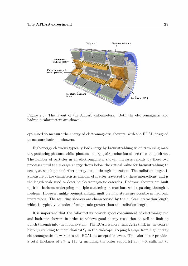
The ATLAS experiment 29
Figure 2.5: The layout of the ATLAS calorimeters. Both the electromagnetic andhadronic calorimeters are shown.
optimised to measure the energy of electromagnetic showers, with the HCAL designed
to measure hadronic showers.
High-energy electrons typically lose energy by bremsstrahlung when traversing mat-
ter, producing photons, whilst photons undergo pair production of electrons and positrons.
The number of particles in an electromagnetic shower increases rapidly by these two
processes until the average energy drops below the critical value for bremsstrahlung to
occur, at which point further energy loss is through ionization. The radiation length is
a measure of the characteristic amount of matter traversed by these interactions, and is
the length scale used to describe electromagnetic cascades. Hadronic showers are built
up from hadrons undergoing multiple scattering interactions whilst passing through a
medium. However, unlike bremsstrahlung, multiple final states are possible in hadronic
interactions. The resulting showers are characterised by the nuclear interaction length
which is typically an order of magnitude greater than the radiation length.
It is important that the calorimeters provide good containment of electromagnetic
and hadronic showers in order to achieve good energy resolution as well as limiting
punch through into the muon system. The ECAL is more than 22X0 thick in the central
barrel, extending to more than 24X0 in the end-caps, keeping leakage from high energy
electromagnetic showers into the HCAL at acceptable levels. The calorimeter provides
a total thickness of 9.7 λI (11 λI including the outer supports) at η =0, sufficient to

The ATLAS experiment 30
control punch-through of hadronic showers into the muon chambers.
2.4.1 Electromagnetic Calorimeter (ECAL)
The ECAL is a lead-LAr detector where lead plates are used to absorb energy, with liquid
argon (LAr) being used as the sampling material. The ECAL exploits a complicated
accordion geometry in order to give complete φ coverage without any azimuthal cracks.
The accordion geometry is shown in more detail in figure 2.6.
The ECAL is divided into a barrel section (covering |η| < 1.475) and two end-caps
(covering 1.375 < |η| < 3.2). The transition region between the barrel and the end-caps
results in a crack in the coverage. The end-cap section of the ECAL is comprised of
two wheels, one covering 1.375 < |η| < 2.5 and the other covering 2.5 < |η| < 3.2. The
central η range (|η| < 2.5) is devoted to precision measurements as this is the η range
where the ECAL is matched to the ID. Here the ECAL is comprised of three longitudinal
layers and has has fine granularity suited to precision measurements of electrons and
photons. For 2.5 < η < 3.2 the ECAL consists of two longitudinal sections with a coarser
granularity. The granularity of the ECAL for different η ranges is summarised in table
2.3. A presampler layer covers the range 0 < |η| < 1.8 giving a measurement of the
energy lost from showers in front of the ECAL in this range.
The ECAL is a non-compensating calorimeter, and as such it responds differently to
electromagnetic and hadronic showers. Calibrations to correct this difference are applied
as part of the offline reconstruction software.
2.4.2 Hadronic Calorimeter (HCAL)
The HCAL is divided into three separate calorimeters:
1. Tile Calorimeter
2. LAr hadronic end-cap calorimeter
3. LAr forward calorimeter (FCAL)
These calorimeters provide coverage out to |η| = 4.9. The reach out to such high
η is important in giving a good missing transverse energy (EmissT ) resolution, whilst

The ATLAS experiment 31
∆ϕ = 0.0245
∆η = 0.02537.5mm/8 = 4.69 mm ∆η = 0.0031
∆ϕ=0.0245x4 36.8mmx4 =147.3mm
Trigger Tower
TriggerTower∆ϕ = 0.0982
∆η = 0.1
16X0
4.3X0
2X0
1500 m
m
470 mm
η
ϕ
η = 0
Strip towers in Sampling 1
Square towers in Sampling 2
1.7X0
Towers in Sampling 3 ∆ϕ×�∆η = 0.0245×�0.05
Figure 2.6: A detailed diagram showing the layout of the electromagnetic calorimeter.

The ATLAS experiment 32
EM Calorimeter
Granularity ∆η×∆φ versus |η|Barrel End-cap
Presampler 0.025× 0.1 |η| < 1.52 0.025× 0.1 1.5 < |η| < 1.8
1st Layer 0.025/8× 0.1 |η| < 1.4 0.050× 0.1 1.375 < |η| < 1.425
0.025× 0.025 1.4 < |η| < 1.475 0.025× 0.1 1.425 < |η| < 1.5
0.025/8× 0.1 1.5 < |η| < 1.8
0.025/6× 0.1 1.8 < |η| < 2.0
0.025/4× 0.1 2.0 < |η| < 2.4
0.025× 0.1 2.4 < |η| < 2.5
0.1× 0.1 2.5 < |η| < 3.2
2nd Layer 0.025× 0.025 |η| < 1.4 0.050× 0.025 1.375 < |η| < 1.425
0.075× 0.025 1.4 < |η| < 1.475 0.025× 0.025 1.425 < |η| < 2.5
0.1× 0.1 2.5 < |η| < 3.2
3rd Layer 0.050× 0.025 |η| < 1.35 0.050× 0.025 1.5 < |η| < 2.5
Table 2.3: A summary table showing details of the granularity of the ECAL in differentpseudorapidity ranges for each layer (including the presampler).
also allowing for the reconstruction of forward tag-jets. As previously mentioned, the
thickness of the HCAL provides good shower containment in order to minimise punch
through into the muon system.
The Tile Calorimeter is a sampling calorimeter comprising layers of iron and scin-
tillating tiles. Ionizing particles crossing the 3 mm scintillator tiles produce ultraviolet
light. This scintillating light is collected and read into photomultiplier tubes along wave-
length shifting fibres. These fibres convert the light from the ultraviolet to the visible
spectrum. The structure of the Tile Calorimeter is separated into barrel (|η| < 1.0) and
extended barrel (0.8 < |η| < 1.7) regions.
The Hadronic end-cap calorimeters are located behind the ECAL end-cap. They
extend from |η| = 1.5 to |η| = 3.2, thereby overlapping with both the Tile Calorimeter
and the FCAL. This is designed to reduce the drop in density in the gaps between the
different sections. Each end-cap consists of two independent wheels, each one built of 32
modules and two longitudinal sections, giving a total of four samplings. The hadronic
end-cap calorimeters use LAr as the active medium between copper plates.

The ATLAS experiment 33
The forward η regions are covered by the FCAL. Due to the longitudinal space
available to the FCAL, it has a high density design, comprising of three modules (one
made of copper, the other two tungsten). Like the ECAL and the hadronic end-cap
calorimeters, LAr is used as the sensitive medium in the FCAL.
2.4.3 Anticipated Calorimeter Performance
ECAL Performance
In order to achieve precise energy measurements in the ECAL, corrections must be
applied to optimise the energy resolution and linearity of response. These corrections
take the form of η-dependent longitudinal weights as follows:
E = s (η) [c (η) + w0 (η) ·EPS + Estrips + Emiddle + w3 (η) ·Eback] (2.2)
where EPS, Estrips, Emiddle and Eback correspond to the measured energies in the pre-
sampler, strip, middle and back layers respectively. s (η) acts as an overall scale factor,
c (η) corrects for any offset, w0 (η) corrects for upstream energy losses and w3 (η) corrects
for longitudinal leakage. The energy resolution (σE/E) can be expressed as a function
containing a stochastic term (a), a noise term (b) and a constant term (c):
σE/E =
√a2
E+b2
E2+ c2 (2.3)
The expected energy resolution has been studied through extensive simulations, val-
idated by results using test-beams. The expected stochastic terms, from simulation,
for the electron and photon energy resolutions are shown for three values of η in ta-
ble 2.4. Test-beam studies as part of the ATLAS Combined Test-Beam (corresponding
to η = 0.4 in ATLAS) give a stochastic term of (9.93± 0.15) % ·√
GeV and a constant
term of 0.2% (after subtraction of the noise term). The ECAL resolution is worse at
larger η compared to the central η region. A significant degradation in energy resolution
occurs in the 1.37 < |η| < 1.52 range where transition between the barrel and end-caps
occurs.

The ATLAS experiment 34
Stochastic Term
Electron Photon
η = 0.3 10.0% 10.2%
η = 1.1 15.1% 12.4%
η = 2.0 14.5% 12.1%
Table 2.4: Expected stochastic terms for the energy resolution of electrons and photonsat η = 0.3, η = 1.1 and η = 2.0.
HCAL Performance
As in the ECAL, the energy resolution of jets reconstructed in the combined calorimeter
system (both the ECAL and HCAL) can be expressed in a three parameter fit involving
stochastic, noise and constant terms. For central jets (0.2 < |η| < 0.4) the stochastic
term is ≈ 60%√
GeV, while the constant term is ≈ 3%. The noise term gives an
important contribution to the overall η-dependence of the jet resolution, increasing from
0.5 GeV to 1.5 GeV between the central barrel region and the end-cap region. This
increase in noise is due to the change from the low-noise tile calorimeter to the LAr
end-cap calorimeters which suffer from higher noise levels.
2.5 Muon System
Muons primarily lose energy through ionization. This, together with the muon lifetime,
means that muons will not be stopped in the ATLAS calorimeters (typically muons with
momenta above ∼ 3 GeV will pass through the calorimeters). In order to reconstruct
muons and measure their momenta, the ATLAS design incorporates a dedicated muon
spectrometer (see figure 2.7), located outside the hadronic calorimeters. This uses the
deflection power of a system of large superconducting air-core toroid magnets, and a
series of tracking chambers to detect and measure the momentum of charged particles
that have passed through the barrel or end-cap calorimeters. These tracking chambers
provide both trigger and precision hit information. In order to achieve a good momen-
tum resolution up to high muon momenta, a large magnetic field over a large distance is
desirable (the ID can provide good measurements for lower momenta tracks, but for mo-
menta & 100 GeV its momentum resolution becomes limited by the relatively small size

The ATLAS experiment 35
of the ID volume). It is anticipated that muons will be identified with momenta above
3 GeV, with precise momentum determination up to transverse momenta of ∼ 3 TeV.
The magnetic field for the muon spectrometer is provided by three air-core toroids
(one barrel toroid and two smaller end-cap toroids). Both the barrel and end-cap toroids
consist of eight “race-track” coils. The coils are made of an Al-stabilised Nb/Ti/Cu
conductor, which is cooled to 4.6 K during operation. The toroids generate an average
magnetic field of ∼ 0.5 T in the barrel (ranging from 0.15 T to 2.5 T), increasing to
∼ 1 T in the end-caps (ranging from 0.2 T to 3.5 T). Good magnetic field coverage is
provided up to |η| ∼ 2.6, however there are regions with low bending power, notably in
the transition region between barrel and end-cap toroids.
The field generated by the toroid magnet system is mainly in the φ-direction, there-
fore providing bending power in the R–z plane. The precision tracking chambers are
optimised to measure the coordinates of the track in the bending R–z plane. In the bar-
rel section the chambers are located parallel to the beam axis in three octagonal shells
at approximate radii of 5 m, 7.5 m and 10 m. In the end-caps, the chambers are located
perpendicular to the beam axis and form large wheels. Typically a muon propagating
out from the interaction point will pass through three muon stations, allowing three
precision measurements to be taken.
A combination of Monitored Drift Tubes (MDTs) and Cathode Strip Chambers
(CSCs) are used for the precision tracking. MDTs are used over most of the pseudo-
rapidity range except for higher pseudorapidities (2.0 < |η| < 2.7) where CSCs are used
for the inner layer. The particle fluxes and radiation levels are highest in this higher
pseudorapidity region, impacting on the muon reconstruction efficiency. Consequently,
the higher granularity CSCs are used in this region.
A requirement of the muon system is the capability to trigger on muon tracks. To
complement the precision tracking chambers, the muon system is instrumented with
a system of fast trigger chambers (the slower response time of the precision chambers
make them unsuitable for triggering). These are designed to return a trigger signal
within a few tens of nanoseconds of a charged particle passing. The trigger chambers
also measure both coordinates of the track, both in the bending and non-bending planes.
The trigger system has full φ coverage and covers the pseudorapidity range of |η| < 2.4,
using Resistive Plate Chambers (RPCs) in the barrel and Thin Gap Chambers (TGCs)
in the end-caps. These allow a trigger signal with a spread of 15 ns to 25 ns to be
delivered, within the trigger requirements for identifying a given bunch crossing.

The ATLAS experiment 36
Figure 2.7: The ATLAS muon system. The different muon chambers are labelled, alongwith the barrel and end-cap toroids of the muon magnet system.
2.5.1 Anticipated Muon Performance
The stand-alone tracks reconstructed by the muon spectrometer are reconstructed over
the range |η| < 2.7. For the region matching the geometrical acceptance of the ID
(|η| < 2.5), these stand-alone tracks are combined with ID tracks to give a combined
muon reconstruction. Combining tracks significantly improves the momentum resolu-
tion for low pT muons where the ID can provide the best measurement. At higher
pT, the muon spectrometer provides the best momentum measurement, allowing recon-
struction of muons with transverse momenta of up to 3 TeV. For low momenta tracks
(below 6 GeV) where muon tracks do not always reach the outer muon chambers, and
in regions where the geometrical acceptance of the muon spectrometer is reduced, the
stand-alone performance is improved by matching ID tracks to track segments in the
muon spectrometer. The fractional momentum resolution is expected to be ≈ 3% for
100 GeV muons and ≈ 10 % for 1 TeV muons. For |η| < 0.1 and 1.1 < |η| < 1.3 (the
transition region between barrel and end-cap where the middle muon stations will be
missing during initial data-taking) the performance is limited by gaps in the coverage of
the muon spectrometer. Some degradation of the performance can also be expected in
regions where support structures and the feet supporting the experiment are found.

The ATLAS experiment 37
2.6 Trigger
At design luminosity of 1034 cm-2s-1 ATLAS will experience a proton-proton interaction
rate of ∼ 1 GHz. The available technology and resources limit the rate of recording
event data to ∼ 200 Hz. Consequently, the trigger system is presented with the chal-
lenge of providing a rejection factor of ∼ 5× 10⁶ against minimum-bias processes while
efficiently recording events corresponding to the new physics processes sought by AT-
LAS. To achieve this goal, the ATLAS trigger system has been designed using a Level-1
(L1) trigger and subsequent high-level trigger (including a Level-2 (L2) trigger and an
event filter (EF)) to reduce the data-taking rate to an acceptable level. Each trigger
level refines the trigger decision made at the previous level.
The L1 trigger uses a subset of the detector information to make a decision in less
than 2.5 µs, reducing the total event rate to 70 kHz (upgradeable to 100 kHz). The L1
trigger forms Regions of Interest (RoIs) from regions within the detector where it has
selected interesting features. The η and φ positions of these RoIs are passed on to the
high-level trigger. Whilst the L1 trigger decision is being formed, the event information
for all the channels is stored in memory pipelines contained in on-detector electronics.
The L2 and EF use an increased amount of detector information in order to make their
refined decisions. The full granularity and precision on all available detector information
in the RoI is used to reduce the event rate to ∼ 3.5 kHz after L2, processing each event
in ∼ 10 ms. The final event rate is reduced to ∼ 200 Hz by the EF. Events passing the
EF are then written to permanent storage with a final event size of ∼ 1.5 MByte.

Chapter 3
SCT Assembly Testing
The ATLAS semiconductor Tracker (SCT) was introduced in chapter 2. This chapter
describes the SCT in more detail, focusing on the SCT barrels and barrel modules and
also discusses the data acquisition (DAQ) system and its use in performance tests during
the macro-assembly of the SCT barrels.
The SCT is geometrically divided into three regions, a barrel region and two end-
caps. The barrel region is made up of four concentric cylindrical layers termed barrels
3 (the innermost layer), 4, 5 and 6 (the outermost layer). Each barrel layer is tiled
with a number of modules (the details of which are described in section 3.2). Rows of
12 modules are mounted parallel to the axis of the barrel cylinder on each barrel, the
number of rows determined by the barrel radius. The modules in a given row are labelled
Z−6 to Z+6 (as shown in figure 3.1), with the two halves of the barrel named Z− and
Z+. The modules are mounted such that they overlap in coverage in both the z- and
rφ-directions, with a tilt angle of ∼ 11◦ allowing overlap between adjacent rows. The
geometry of the barrels and the numbers of modules on each layer are summarised in
table 3.1. The barrel support-structures are made of lightweight carbon-fibre reinforced
plastic, and support both the modules and the services (low-mass tapes (LMTs) to
distribute power, cooling loops and optical data links). The modules were mounted
onto the barrel carbon-fibre support-structures during a macro-assembly phase, with
the completed barrels later shipped to CERN for integration with the rest of the Inner
Detector.
38

SCT Assembly Testing 39
Barrel Number Radius / mm Length / mm Rows Modules
Barrel 3 299 1492 32 384
Barrel 4 371 1492 40 480
Barrel 5 443 1492 48 576
Barrel 6 514 1492 56 672
Table 3.1: The barrel radius and number of modules for each of the four SCT barrellayers.
−3 −1 +1 +2−6 −5 −4 −2 +3 +4 +5 +6
Z− Z+
Figure 3.1: A diagram showing the module position numbering convention for a row ofmodules mounted on an SCT barrel. A single row of 12 modules is shown. Rows aredefined parallel to the z-axis. The barrel is separated into two halves, labelled Z− andZ+.
3.1 Semiconductor detectors
Semiconductors have a small energy gap between the occupied ‘valence band’ energy
levels and the next available energy levels (in the ‘conduction band’). In silicon the
energy required to promote an electron from the valence band to the conduction band
is 3.6 eV1. The properties of semiconductors can be controlled through the process of
doping, whereby group V or group III atoms are introduced to the semiconductor (silicon
in this case), displacing silicon atoms from some of the atomic sites in the lattice. The
addition of group V atoms (termed ‘donors’) contribute extra electrons at energy levels
just below the conduction band, producing an ‘n-type’ semiconductor. Dopants from
group III atoms (termed ‘acceptors’) introduce an empty energy level just above the
valence band which can readily be filled by a valence electron to introduce a hole. Such
semiconductors are known as ‘p-type’.
Bringing these two types of doped semiconductor together results in a p-n junction. A
1This is larger than the actual band gap in silicon which, as an indirect band gap semiconductor,also requires an associated phonon excitation to conserve momentum when making a transition.

SCT Assembly Testing 40
gradient in the charge-carrier density across the interface causes the diffusion of electrons
and holes into the p- and n-type regions respectively. The diffusion of electrons leaves
behind fixed positively-charged donor ions, whereas the diffusion of holes leaves behind
fixed negatively-charged acceptor ions, resulting in regions of net charge either side of
the junction with no mobile charge carriers (a region known as the depletion region).
At equilibrium the potential difference across this region is called the ‘contact potential’
and its direction is such that it acts to prevent further diffusion of electrons into the p-
type region and holes into the n-type region. Any electron-hole pairs created inside this
depletion region will be swept out of the depletion region by the electric field associated
to the contact potential, giving the basis of an electric signal.
When electrons or holes are liberated in a semiconductor they will migrate (either
spontaneously or under the influence of an applied electric field) until they either re-
combine or are collected at an electrode. In the interests of efficient particle detection,
it is important to prevent recombination or other mechanisms of carrier loss2 as they
will reduce the measured pulse height. Consequently, it is important to have a short
enough collection time for carriers such that it is sufficiently less than the recombination
lifetime.
So far, a junction with no applied external voltage has been considered. Such a junc-
tion will function as a particle detector [22], however the performance of such a device
can be significantly improved by applying a reverse bias. An unbiased junction has a
low contact potential and therefore any introduced charge (such as the ionization from
a passing charged particle) will not move very quickly under the effect of the contact
potential alone. Consequently charge carriers will be readily lost to recombination and
trapping. By applying an external voltage, so as to reverse bias the junction, the po-
tential difference across the junction is increased and the width of the depletion region
increases either side of the junction. The reverse biased p-n provides a more effective
detector as charge carriers created within the larger depletion region can be quickly and
efficiently collected. A schematic diagram of a silicon microstrip detector is shown in
figure 3.2.
The properties of silicon after irradiation are very important in a silicon detector,
particularly at the LHC where, for 10 years of running, the SCT needs to withstand an
2The presence of ‘deep impurities’ (unlike the deliberate dopant impurities) can act as recombinationcentres that can capture both electrons and holes allowing them to recombine. Other defects in crystalscan cause charge carriers to become trapped, immobilising the carrier for a period of time long enoughto prevent the carrier contributing to the measured pulse.

SCT Assembly Testing 41
� � �� � � � � �� � � � � �� � �
Al
charged particle
holes
electons
����������������������������������������������������������������������������������������������������������
�������������������� �������������������������������������������� � � � � � � � � � � � �
��������������������������P P P
n−type
Al Electrode 80 um
22 um
Si O2
N+
E−field
285 um
Figure 3.2: A schematic diagram showing a cross-section through a silicon microstripdetector. Strips of p-type semiconductor are formed on a bulk n-type semiconductor.The dimensions shown correspond to those used in the ATLAS SCT barrel sensors.Diagram taken from [23].
expected fluence3 of ∼ 2× 10¹⁴ (1 MeV neq) cm−2. The irradiation of a lightly doped,
n-type silicon can change the properties such that, with time, it type-inverts, becoming
increasingly p-type. This reduces the contact potential across the junction, requiring an
increased bias voltage to maintain detector performance. The sensors used in the SCT
barrel modules are of type (p+, n, n+)4 (as shown in figure 3.2), and after irradiation
can be expected to undergo type inversion such that they appear (p+, p, n+). Radi-
ation damage can increase leakage currents in the silicon, resulting in increased noise
levels. The leakage currents dissipate heat into the detector, which in turn can induce
further leakage currents5, leading to the threat of thermal run-away. Irradiated silicon
is also susceptible to a detrimental process known as “reverse annealing”. The effects of
radiation damage are strongly temperature-dependent, and can be controlled by main-
taining the sensors at a low temperature. In ATLAS, the SCT sensors will be kept at a
temperature of ∼ − 7 ◦C throughout their operation.
3The dose quoted here is normalized to that of 1 MeV neutrons.4p+ and n+ denote heavily doped p-type and n-type semiconductors respectively.5Leakage currents can be induced through thermally produced electron-hole pairs

SCT Assembly Testing 42
Figure 3.3: A labelled diagram of an SCT barrel module. The length of the module is128 mm. Figure taken from [24]
3.2 SCT barrel module design
An SCT barrel module [24] (shown in figures 3.3 and 3.4) incorporates silicon wafers,
comprising p-n junctions under reverse bias, as the sensor element. The electron-hole
pairs liberated by passing charged-particles are swept towards the electrodes at the
opposite sides of the junction. These p-n junctions are produced in strips on the surface
of the silicon wafers (285 µm thick) using a p-strip on n-bulk design, with a strip pitch
of 80 µm. The wafers for all barrel modules are identical, with a rectangular geometry
(64 mm by 63.6 mm) and comprising 768 strips [25]. Each module is made of four wafers
in two layers (each layer being formed from two wafers connected end-to-end). The two
layers are offset by a small stereo angle of 40 mrad in order to give a measurement in the
z-direction (given that one layer is aligned along the z-direction in order to give precise
measurements in the R-φ direction). The pair of sensors on each barrel module allow a
nominal position resolution of 17 µm in the R-φ direction and 580 µm in the z-direction.
The strips are read out by application specific integrated circuits (ASICs) known as
ABCD3TAs [26]. These ‘front-end’ ASICs each read out 128 channels, so 12 chips are
used to read out all of the channels on a SCT module. The 12 ASICs are mounted on
a wrap-around electronic hybrid, each side of the hybrid holding six ASICs (the six on
the top side termed ‘link-0’ and the six on the bottom side termed ‘link-1’, in reference

SCT Assembly Testing 43
Figure 3.4: A photograph showing several SCT barrel modules as mounted on a barrelsupport-structure.
to their corresponding optical read-out link). Each side has one master chip that is
responsible for transmitting all the data from that side off the module. In the event of
a chip failure, it can be bypassed so that the remaining data can be read out. Should a
master chip fail then the remaining chips on that link can be read out through the other
link, giving a level of redundancy.
A significant feature of the ABCD3TA chip design is the use of a binary readout.
This means that the only pulse-height information transmitted by the ASICs is a single
bit per channel denoting that the pulse was above a set threshold. The discriminator
threshold is a configurable parameter on the ABCD3TA. Ensuring that the calibration
of this threshold is correct is very important as no further pulse-height information is
transmitted off the module, and cannot be recovered later. The discriminator should be
set at a level that ensures a good efficiency at registering genuine hits whilst maintaining
a low noise occupancy level. The module design specifications require that the noise
occupancy per strip is < 5× 10⁻⁴ with an efficiency > 99 %.
A charged particle passing through the silicon detector deposits a small amount of
charge according to a Landau distribution [27]. Imperfections in the charge collection and
other sources of noise will adjust the shape of this distribution. At the stage where the
measured collected charge is seen by the threshold discrimination circuit, the distribution
can instead be described by the improved distribution given by a Landau convolved with
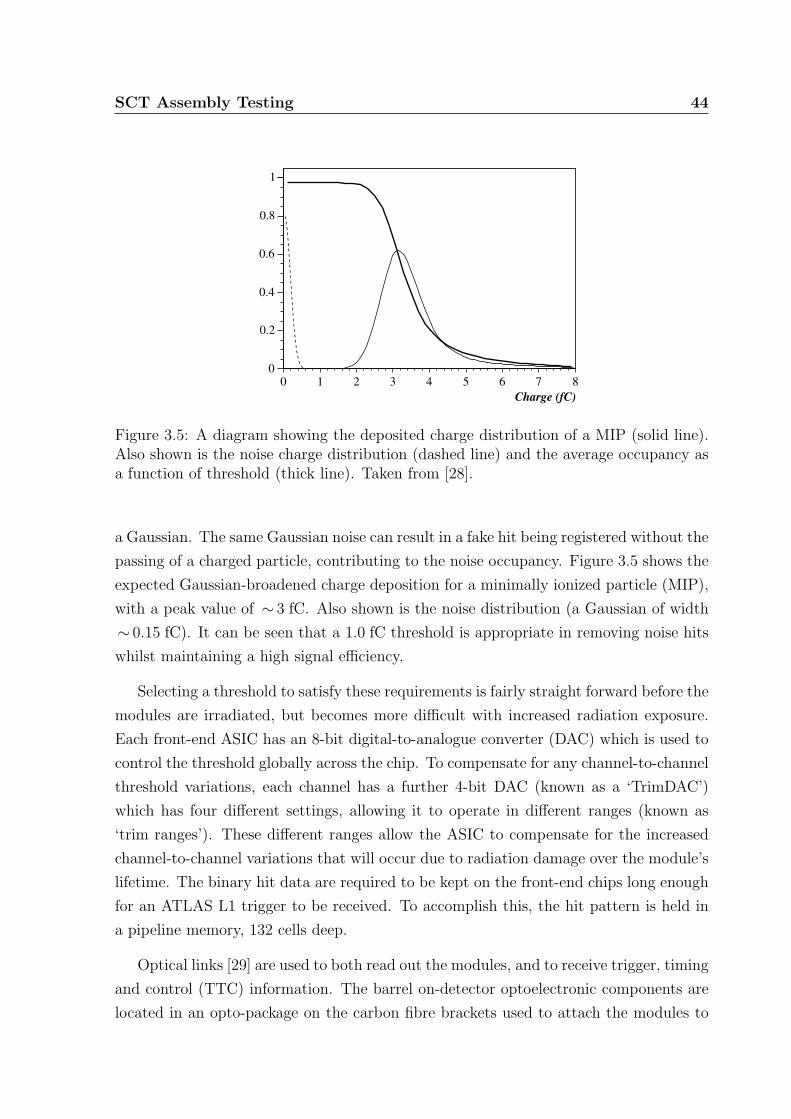
SCT Assembly Testing 44
Charge (fC)0 1 2 3 4 5 6 7 8
0
0.2
0.4
0.6
0.8
1
Figure 3.5: A diagram showing the deposited charge distribution of a MIP (solid line).Also shown is the noise charge distribution (dashed line) and the average occupancy asa function of threshold (thick line). Taken from [28].
a Gaussian. The same Gaussian noise can result in a fake hit being registered without the
passing of a charged particle, contributing to the noise occupancy. Figure 3.5 shows the
expected Gaussian-broadened charge deposition for a minimally ionized particle (MIP),
with a peak value of ∼ 3 fC. Also shown is the noise distribution (a Gaussian of width
∼ 0.15 fC). It can be seen that a 1.0 fC threshold is appropriate in removing noise hits
whilst maintaining a high signal efficiency.
Selecting a threshold to satisfy these requirements is fairly straight forward before the
modules are irradiated, but becomes more difficult with increased radiation exposure.
Each front-end ASIC has an 8-bit digital-to-analogue converter (DAC) which is used to
control the threshold globally across the chip. To compensate for any channel-to-channel
threshold variations, each channel has a further 4-bit DAC (known as a ‘TrimDAC’)
which has four different settings, allowing it to operate in different ranges (known as
‘trim ranges’). These different ranges allow the ASIC to compensate for the increased
channel-to-channel variations that will occur due to radiation damage over the module’s
lifetime. The binary hit data are required to be kept on the front-end chips long enough
for an ATLAS L1 trigger to be received. To accomplish this, the hit pattern is held in
a pipeline memory, 132 cells deep.
Optical links [29] are used to both read out the modules, and to receive trigger, timing
and control (TTC) information. The barrel on-detector optoelectronic components are
located in an opto-package on the carbon fibre brackets used to attach the modules to

SCT Assembly Testing 45
the barrel structure. In total, each module has three optical links, two of which act as
readout links, and one of which is used to receive TTC signals. As already mentioned,
the two readout links provide a redundancy mode in case of a failure along one of the
links. Redundancy is also built into the TTC link whereby an electrical control line can
be set to receive a copy of the TTC signal from a neighbouring module in case of a TTC
signal failure.
Data leaving a module are passed, via a VDC6, to a VCSEL (Vertical Cavity Surface
Emitting Laser) within the opto-package. This VCSEL produces the optical signal that
is transmitted off-detector. Optical signals arriving at the opto-package are received by
a p-i-n diode. Here the signal is converted from optical to electrical form, and passed to
the DORIC4A ASIC which decodes the TTC data for further transmission to the front-
end ASICs. The connections between the opto-packages and the off-detector electronics
are through optical fibres. The fibres transmitting TTC commands to the modules are
called TX fibres, and those receiving data from the modules are known as RX fibres. To
ensure that data are successfully transmitted across the optical links, RX and TX DAC
thresholds are set at optimal values to ensure a sufficiently small (< 10−9) bit error rate.
3.3 Data Acquisition
The SCT Data Acquisition (DAQ) system [30] is used to configure the module ASICs,
communicate trigger information and transfer data from the front-end chips on each
module. The DAQ system is also used in calibrating the detector through a series
of functional tests that can test the operation of the modules and optimise the module
configurations. The SCT DAQ readout hardware consists of several different components
(see figure 3.6), including:
Read Out Drivers (RODs) — RODs provide the main module configuration, control
and data handling.
Back Of Crate (BOC) boards — These control the input and output to and from
the front-end modules (via TX and RX optical fibres) for the RODs and also
provide a link to the central ATLAS DAQ. Each ROD has a complementary BOC
board, and services 48 modules.
6The VCSEL Driver Chip (VDC) is a custom ASIC used to provide the required signal to drive theVCSEL

SCT Assembly Testing 46
ROD CrateBusy
RODCrate
Controller
(RCC)
TTCInterfaceModule
(TIM)
Read OutDriver
(ROD)
Back OfCrate
(BOC)
VME
o
TTC(optical)
x16/crate x16/crate
Backplane Connections
o
Clock andControl (optical)48/BOC
o96/BOC
Data (optical)FrontEnd
Modules
o
Formatted data(optical)
Slink(1/BOC)
ROS(ATLASCentralDAQ)
ROD Busy
40 MHz Clock
ATLASTrigger System
FastCommands
And Serialised IDs
Figure 3.6: A block diagram showing the components of the SCT data acquisitionhardware. The main connections between the components are also shown. Figure takenfrom [30].
TTC Interface Module (TIM) — The TIM is used to accept trigger, timing and
control (TTC) signals that are received from ATLAS, and distribute them on to
the RODs/BOCs. The TIM can also be used to generate TTC information itself.
ROD Crate Controller (RCC) — The RCC is a rack mounted Linux PC that con-
figures and controls the functions of the other readout components within a crate.
Each crate contains one RCC, one TIM and up to 16 ROD/BOC pairs (reading
out up to 768 modules).
The SCT has two main modes of operation (i) physics data-taking mode, and (ii)
calibration mode. In physics data-taking mode, the TIM receives triggers from the
central ATLAS trigger system. They are then passed on to each of the RODs. Each
ROD communicates these signals through its BOC and on to the front-end modules. The
BOC receives the corresponding hit information from the modules and data formatting
takes place on the ROD. The data are passed from the ROD (through the BOC again)
and into the main ATLAS DAQ system.

SCT Assembly Testing 47
In calibration mode, the SCT DAQ can operate without communication to the central
DAQ and without receiving triggers from the ATLAS trigger system. Instead, the TIM
is used to generate the TTC signal, and triggers can either be sent from the RODs or
from the TIM (if synchronization between the triggers is required). The ROD is used to
sample and histogram the data, with the resultant histograms passed through the RCC
and on to PC servers for analysis.
3.4 Macro-Assembly and DAQ Testing
Macro-assembly of the SCT barrels took place at Oxford (the macro-assembly site)
between June 2004 and August 2005. During this period, SCT barrel modules were
systematically mounted onto the barrel support-structures. This process was carried
out using custom robots [31] as the space between modules was very restricted (approx-
imately 1.6 mm in the region where adjacent modules overlap) and required that the
modules followed a very precise path as they were mounted, in order to prevent damage
to neighbouring modules.
An important part of the macro-assembly process involved running a series of DAQ
tests to check that the modules were successfully mounted, to measure their noise occu-
pancy, to confirm any known problem channels and to check for any new defects that
may have been introduced during the assembly process. A more detailed discussion of
the testing procedure and descriptions of the individual tests can be found in [30, 32–34].
Typically these tests were run at suitable gaps in the module mounting schedule where
∼ 24 newly mounted modules would be tested. The regular testing was carried out
under “warm” conditions, where a C4F10 cooling system was used and the temperature
on the modules (measured on the hybrids when powered) would be ∼ 28 ◦C. When the
module-mounting was completed for a barrel, the entire barrel was again tested7. At
this a point the assembly schedule allowed for a limited period of colder testing where a
C3F8 cooling system (similar to the final cooling system used in ATLAS) was used and
the modules were tested at temperatures of ∼ 12 ◦C (when powered). During this cold-
testing period, the main purpose of the testing was to identify any gross errors affecting
modules such that they may be corrected before the completed barrel was shipped to
CERN (the macro-assembly site being better equipped for the removal and remounting
of modules).
7Schedule constraints meant that barrel 5 was shipped to CERN before a complete test was madeat the macro-assembly site. A full series of tests were performed on reception at CERN.

SCT Assembly Testing 48
The DAQ testing procedure (using the final DAQ electronics and power supplies)
involved several different tests designed to check different aspects of the DAQ module
readout. First, a series of basic tests was run on the modules to check the lines of
communication with the ASICs. These tests checked that the modules could see the
clock signal, receive configuration signals and be put into data-taking mode. The ability
to respond to a “Hard Reset” signal was also tested. An RX threshold test was run
to establish a safe threshold whereby the optical signal could be reliably converted
into electrical form by the data receiver on the BOC. Having established successful
communication with the modules, a series of digital tests were then run in order to
check for stuck pipelines (resulting in channels being “stuck on” or “stuck off” causing
excess noise occupancy or inefficiency respectively), for chip-counter faults and to test
that ASICs could be bypassed (a redundancy feature of the module design allows that in
the event of a chip failure, the data from the remaining chips can be read out, bypassing
the faulty chip).
The testing procedure then incorporated a series of tests aimed at calibrating the
front-end electronics. These calibration tests would typically make occupancy mea-
surements whilst varying a chip parameter (such as the threshold). Each channel has a
capacitor that can be used to inject test charges. Threshold scans performed for different
known injected charges were used to calibrate the discriminator threshold (allowing the
threshold to be calculated in units of input charge). Further scans were used to optimise
the TrimDAC settings to minimise channel-to-channel variations in the threshold.
Two of the DAQ tests that were carried out during barrel assembly were the NoiseOc-
cupancy and the related SynchTriggerNoise tests. In addition to participating in the
running of DAQ test shifts, both during the module-mounting process and during tests
on the full barrels, the author was responsible for the initial analysis of the SynchTrig-
gerNoise data taken during the cold testing at the macro-assembly site. The cold testing
of the barrels at the macro-assembly site provided the first data from running the com-
pleted barrels under cold conditions, an important first check of the performance of the
mounted modules. This is illustrated by the analysis of the first SynchTriggerNoise data
for barrels 3 and 6, presented in section 3.5.
The NoiseOccupancy test is a threshold scan without any injected charge. For each
threshold the noise occupancy is determined. The occupancy due to noise at 1 fC is
recorded as a reference point. The SynchTriggerNoise is designed to test the noise
occupancy when triggers are simultaneously sent to all configured modules. Like the
NoiseOccupancy test, the noise occupancy is measured with no injected charge, however

SCT Assembly Testing 49
triggers are now sent synchronously, by the TIM to the modules, at a high trigger
rate (up to 100 kHz). The purpose of the SynchTriggerNoise test is to look for signs
of elevated noise occupancy when sending triggers to multiple modules synchronously,
checking for any correlated noise effects that would not show up when testing modules
individually or in smaller groups.
3.5 Initial SynchTriggerNoise Analysis
The analysis of the data from SynchTriggerNoise tests carried out during the macro-
assembly cold testing of barrels 3 and 6 served two main purposes:
i. to search for signs of any correlated noise effects that are present when running a
large number of modules with high-rate synchronous triggers
ii. to identify any gross problems with modules or any defects and to provide a cross-
check with the other DAQ tests
For a given module, the outputted raw data from the SynchTriggerNoise test contains
histograms (produced on the ROD) giving the number of hits for each of the module’s
1536 channels as a function of time (in bins of 1 s). The number of triggers per time bin,
the number of time bins and the nominal threshold can be adjusted. By knowing the
rate of triggers sent to the modules and the histogramming factor (the histogramming
code allowed for only 1 in every 15 triggers to be histogrammed), the channel occupancy
is given by:
Channel Occupancy =No. Hits on Channel
No. Triggers per Time Bin×No. Time Bins/15(3.1)
During the macro-assembly testing, an error in the SynchTriggerNoise test caused
fewer triggers to be sent to the modules than were requested. Tests requesting 1× 10⁶
triggers per second actually sent only 16960 per second, where tests requesting 2× 10⁵
triggers per second actually sent 3392 per second8. The following results have been cor-
rected accordingly. This lower trigger rate was not ideal for the purpose of testing for
8The TIM was configured to send a 16-bit number rather than the 32-bit number that the SynchTrig-gerNoise test requested. Consequently the 32-bit number was truncated resulting in fewer triggers beingsent than were requested. This was later corrected.

SCT Assembly Testing 50
any differences associated with sending synchronous triggers compared to sending asyn-
chronous triggers as such differences are expected to be more significant when running
at high trigger rates.
3.5.1 Barrel 3 SynchTriggerNoise Analysis
Two SynchTriggerNoise tests were performed on the first barrel to be completed, barrel
3, during cold testing (runs 2177.5 and 2177.6). The two tests were performed for
different numbers of triggers and thresholds. Run 2177.5 sent 3392 triggers per time bin
with a threshold set at 0.9 fC. Run 2177.6 had a threshold of 1.0 fC with 16960 triggers
per time bin. One ROD failed during these tests, resulting in the loss of data from 48
modules (out of a total of 384 modules on barrel 3). A further module was removed
from the configuration due to a fault and was later replaced.
Considering data from run 2177.6 at a nominal threshold of 1.0 fC, figure 3.7 shows
the mean channel occupancy per module, and also the mean channel occupancy over
link-0 and link-1 of each module. It can be seen that the mean channel occupancies for
all modules are within the design specification (< 5× 10⁻⁴ at a threshold of 1.0 fC) with
the majority of modules exhibiting mean channel occupancies of less than 5× 10⁻⁵. The
highest mean channel occupancy is 1.16× 10⁻⁴. One can see that the mean occupancy
is typically higher on link-1 than on link-0 of the modules (this is an intrinsic property
of the modules). During the analysis of these data, individual chips with either high
noise levels or zero-noise were identified as these could be indications of problems with a
given module. Figure 3.8 shows the mean channel occupancy per module mapped over
the module position on the barrel. The positions of the 49 modules for which no data
were taken can clearly be seen.
To investigate whether the sending of synchronous triggers caused any global in-
crease in noise levels, the SynchTriggerNoise occupancies were compared to those from a
NoiseOccupancy test (with asynchronous triggers). Figure 3.9 shows the mean channel
occupancy, calculated from the NoiseOccupancy test data (for a threshold of 1.0 fC),
as a function of position on the barrel. Comparing this with figure 3.8, it can be seen
that the pattern of noisy modules is very similar, showing no signs of correlations in
the SynchTriggerNoise data that weren’t present in the NoiseOccupancy test. To get a
qualitative measure of the change in noise occupancy when sending synchronous triggers,
the ratio F is defined as

SCT Assembly Testing 51
Mean channel occupancy0 0.02 0.04 0.06 0.08 0.1 0.12
-310×
Entri
es
1
10
Entries 335Mean 1.405e-05RMS 1.409e-05
Run 2177.6 at 1.0 fCModule Mean
(a) Mean channel occupancy over entire module
Mean channel occupancy0 0.02 0.04 0.06 0.08 0.1 0.12 0.14
-310×
Entri
es
1
10
Entries 335Mean 1.308e-05RMS 1.514e-05
Run 2177.6 at 1.0 fCLink-0 Mean
(b) Mean channel occupancy over link-0
Mean channel occupancy0 0.02 0.04 0.06 0.08 0.1 0.12 0.14 0.16 0.18 0.2
-310×
Entri
es
1
10
Entries 335Mean 1.501e-05RMS 1.66e-05
Run 2177.6 at 1.0 fCLink-1 Mean
(c) Mean channel occupancy over link-1
Figure 3.7: Mean channel occupancy per module over (a) the entire module, (b) link-0and (c) link-1. The data correspond to a SynchTriggerNoise test run on barrel 3 with anominal threshold of 1.0 fC (run 2177.6).

SCT Assembly Testing 52
Z-position
Z-6
Z-5
Z-4
Z-3
Z-2
Z-1
Z+1
Z+2
Z+3
Z+4
Z+5
Z+6
Row
num
ber
0
5
10
15
20
25
30
Entries 335
Nois
e O
ccup
ancy
0
0.02
0.04
0.06
0.08
0.1
-310×Entries 335Barrel 3 : SynchTriggerNoise Test Results at 1.0fC
Figure 3.8: Mean channel occupancy per module as a function of barrel position for aSynchTriggerNoise test at 1.0 fC for barrel 3 (run 2177.6). The azimuthal rows of thecylindrical barrel (denoted by the row number) are shown unfolded and labelled by therelevant row number.

SCT Assembly Testing 53
F =SynchTriggerNoise Occupancy at 1.0 fC
NoiseOccupancy Occupancy at 1.0 fC(3.2)
This ratio allows one to identify any significant changes in occupancy between the
two runs. It should be noted that changes in the run conditions between the two sets
of tests, such as the module temperatures and the time the modules had been powered,
can be expected to have an impact on the relative noise occupancy values.
Figure 3.10 shows the distribution of F for all modules on barrel 3. This shows a
narrow distribution with a mean of 1.03 but with a small number of isolated modules
displaying occupancies up to 4.5 times greater in the SynchTriggerNoise test than in
the unsynchronised NoiseOccupancy test. Figure 3.11 shows how F varies with module
position on the barrel, with only four modules seen to have significant differences of
F > 2. On inspection of these modules, one module (row 29, Z−6) was identified as
having a “noise slope” defect (a rare condition in which the module shows an increasing
noise occupancy over the last chips on link-1)[33]. This condition was found to be cured
when the neighbouring module was set to receive the redundant TX signal, resulting in
good noise performance. Each of the other three modules had a single bad channel with
high noise occupancy (two modules had a stuck pipeline defect) and weren’t seen as
significant problems. No large scale correlation between module position and increased
noise can be seen.
A second SynchTriggerNoise test was carried out on barrel 3. Run 2177.5 sent 3392
triggers per time bin with a nominal threshold of 0.9 fC. Since run 2177.5 was carried
out at a lower threshold than run 2177.6, one can expect a greater noise occupancy.
This is seen in the plot of mean channel occupancy per module for run 2177.5, shown
in figure 3.12(a). At this threshold, almost all modules have an occupancy less than
2.5× 10⁻⁴, with a small number of modules having higher occupancies (up to 4.2× 10⁻⁴).
Despite the lower threshold, this is still within the design specifications (at 1.0 fC).
Figure 3.12(b) shows a map of the mean channel occupancy per module with position
on the barrel. Comparing this with the equivalent plot for 2177.6 (figure 3.8), one can
see that the pattern of relatively noisy modules is very similar to the pattern for run
2177.6 at the higher threshold. Again, no significant correlation is seen.

SCT Assembly Testing 54
Z-position
Z-6
Z-5
Z-4
Z-3
Z-2
Z-1
Z+1
Z+2
Z+3
Z+4
Z+5
Z+6
Row
num
ber
0
5
10
15
20
25
30
Entries 383
Nois
e O
ccup
ancy
0
0.02
0.04
0.06
0.08
0.1
-310×Entries 383Barrel 3 : NoiseOccupancy Test Results at 1.0fC
Figure 3.9: Mean channel occupancy per module as a function of position on the barrelfor the NoiseOccupancy test. This test sends non-synchronised triggers and recordsthe occupancy at a nominal threshold of 1.0 fC. The azimuthal rows of the cylindricalbarrel (denoted by the row number) are shown unfolded and labelled by the relevantrow number. All RODs were operational during this run.
Entries 335Mean 1.028RMS 0.2456
Fractional Noise change, F0.5 1 1.5 2 2.5 3 3.5 4 4.5
Entri
es
1
10
210 Entries 335Mean 1.028RMS 0.2456
Barrel 3
Figure 3.10: Occupancy ratio, F, comparing the SynchTriggerNoise test (synchronisedtriggers) with the NoiseOccupancy test (non-synchronised triggers). The mean value ofthe occupancy ratio 〈F 〉 = 1.028.

SCT Assembly Testing 55
Z-position
Z-6
Z-5
Z-4
Z-3
Z-2
Z-1
Z+1
Z+2
Z+3
Z+4
Z+5
Z+6
Row
num
ber
0
5
10
15
20
25
30
Frac
tiona
l Noi
se C
hang
e, F
0
0.5
1
1.5
2
2.5
3
3.5
4
Barrel 3 : Fractional Change in Occupancy
Z-position
Z-6Z-5Z-4Z-3
Z-2Z-1
Z+1Z+2Z+3Z+4Z+5
Z+6 Row number
05
1015
2025
30
Frac
tiona
l Noi
se C
hang
e, F
00.5
11.5
22.5
33.5
44.5
Figure 3.11: The variation of the noise occupancy ratio, F , with position on barrel 3. Asmall number of modules show a significant increase in noise occupancy.

SCT Assembly Testing 56
Mean channel occupancy0 0.05 0.1 0.15 0.2 0.25 0.3 0.35 0.4 0.45
-310×
Entri
es
1
10
Entries 335Mean 6.37e-05RMS 5.341e-05
Run 2177.5 at 0.9 fCModule Mean
(a) Mean channel occupancy per module
Z-position
Z-6
Z-5
Z-4
Z-3
Z-2
Z-1
Z+1
Z+2
Z+3
Z+4
Z+5
Z+6
Row
num
ber
0
5
10
15
20
25
30
Entries 335
Nois
e O
ccup
ancy
0
0.05
0.1
0.15
0.2
0.25
0.3
0.35
0.4
-310×Entries 335Barrel 3 : SynchTriggerNoise Test Results at 0.9fC
(b) Mean channel occupancy per module as a function of posi-tion on barrel 3
Figure 3.12: Mean channel occupancies for modules on barrel 3 for a SynchTriggerNoisetest (run 2177.5 with a threshold of 0.9 fC).

SCT Assembly Testing 57
3.5.2 Barrel 6 SynchTriggerNoise Analysis
As with the barrel 3 cold tests, two runs of the SynchTriggerNoise test were performed
on barrel 6, the second barrel to be completed, one test at 1.0 fC with 16960 triggers per
time bin (run 5913.0), and one at 0.9 fC with 3392 triggers per time bin (run 5913.1).
Unfortunately there were readout errors in the data from modules on the Z− half of the
barrel (see figure 3.13). The impact on run 5913.0 involved all modules on Z− failing to
read out any data for 41 bins (out of 51). For run 5913.1 only the first data bin (out of
21) was lost. The very tight schedule pressure prevented repeat tests being run during
the cold-testing period at the macro-assembly site. Despite the data errors for the Z−half of the barrel, the data for runs 5913.0 and 5913.1 were analysed to check for any
chip or channel errors.
During the cold tests of barrel 6, one module lost bias on link-1 (with serial number
20220330200858 at row 7, Z+5) resulting in very high occupancy on this link. This
was clearly observed in the SynchTriggerNoise data (see figure 3.14). This module
was replaced after cold testing and consequently has been removed from the following
analysis. A further seven modules were left out of the test due to problems configuring
them during the limited time available for cold testing.
The mean channel occupancy per module for run 5913.0 is shown in figure 3.15(a).
The mean occupancy over all modules is 2.51× 10⁻⁵, within the design specifications at
1.0 fC. However nine modules are seen to have mean occupancies greater than 5× 10⁻⁴.
Of these modules, seven had mean occupancies of ∼ 6–6.7× 10⁻⁴ due in each case to
a single channel with very high noise levels, and one module with mean occupancy of
∼ 1.2× 10⁻³ as a result of two channels with very high noise levels. The occupancy
for these modules would be significantly reduced by masking off these noisy channels.
A further module had a noise occupancy of ∼ 7× 10⁻⁴ and was found to have a noise
slope resulting in excessive noise on the last two chips on link-1. Figure 3.15(b) shows
the corresponding map of mean channel occupancy per module as a function of module
position. No correlations between noise occupancy levels and position are seen
The corresponding occupancy values for run 5913.1 at the lower threshold of 0.9 fC
are shown in figure 3.16. The higher overall mean occupancy of 7.3× 10⁻⁵ is expected
due to the lower threshold. Again, no large scale correlation of occupancy with position
on the barrel is observed.

SCT Assembly Testing 58
Channel0 100 200 300 400 500 600 700
Tim
e (s
)
0
10
20
30
40
50
0
0.2
0.4
0.6
0.8
1
1.2
1.4
1.6
1.8
2
5913.0: Module 20220040200585 Link-0
Channel0 100 200 300 400 500 600 700
Tim
e (s
)
0
10
20
30
40
50
0
0.2
0.4
0.6
0.8
1
1.2
1.4
1.6
1.8
2
5913.0: Module 20220040200585 Link-1
Channel0 100 200 300 400 500 600 700
Tim
e (s
)
0
5
10
15
20
02
4
6
8
10
12
14
16
18
2022
5913.1: Module 20220040200125 Link-0
Channel0 100 200 300 400 500 600 700
Tim
e (s
)
0
5
10
15
20
0
20
40
60
80
100
120
140
160
180
200
5913.1: Module 20220040200125 Link-1
Figure 3.13: Examples of errors in the raw data for runs 5913.0 and 5913.1 for moduleson Z−. The histograms show the number of hits registered on a given channel as afunction of time, with the divisions between ASICs shown by dashed lines. For run5913.0 at 1.0 fC, all modules on Z− lost data from the 10th bin onward. For run 5913.1at 0.9 fC only the first bin for modules on Z− was lost.

SCT Assembly Testing 59
Channel0 100 200 300 400 500 600 700
Tim
e (s
)
0
5
10
15
20
0
0.1
0.2
0.3
0.4
0.5
0.6
0.7
0.8
0.9
1
5913.1: Module 20220330200358 Link-0
Channel0 100 200 300 400 500 600 700
Tim
e (s
)
0
5
10
15
20
0
2
4
6
8
10
12
14
5913.1: Module 20220330200358 Link-1
Figure 3.14: Module 20220330200358 lost bias on one half of the module during the coldtests and was later replaced. The high noise occupancy can clearly be seen on link-1 ofthis module.
3.6 Summary
The initial SynchTriggerNoise test data taken during cold testing of barrels 3 and 6 of
the SCT, before their shipment to CERN, have been analysed. The analysis of barrel 3
data showed no large scale increase in noise occupancy levels when sending synchronous
triggers, compared to non-synchronous triggers. Overall, the noise occupancy levels on
barrel 3 were within the design specifications, and no signs of correlated noise effects
were seen.
The SynchTriggerNoise raw data for barrel 6 was affected by readout errors, meaning
that there was not a complete set of data for the whole barrel. The analysed data show
no obvious correlations of noise occupancy with position on the barrel. A small number
of modules had higher noise occupancies than the specifications, due to individual noisy
channels and in one case excessive noise on a single chip. Masking off the defective
channels would improve the mean module occupancy in these cases. Overall, noise
occupancy levels are seen to be within design specifications and no large scale correlations
of noise occupancy due to synchronous triggers were seen.
The analysis of these initial data demonstrated the use of DAQ tests in detecting
problem channels and module defects, along with module calibration. With the success-
ful completion of the macro-assembly phase, the results of the DAQ tests were able to

SCT Assembly Testing 60
Mean channel occupancy0 0.2 0.4 0.6 0.8 1 1.2
-310×
Entri
es
1
10
210
Entries 664Mean 2.51e-05RMS 8.699e-05
Run 5913.0 at 1.0 fCModule Mean
(a) Mean channel occupancy per module
Z-position
Z-6
Z-5
Z-4
Z-3
Z-2
Z-1
Z+1
Z+2
Z+3
Z+4
Z+5
Z+6
Row
num
ber
0
10
20
30
40
50
Entries 664
Nois
e O
ccup
ancy
0
0.2
0.4
0.6
0.8
1
1.2-310×
Entries 664Barrel 6 : SynchTriggerNoise Test Results at 1.0fC
(b) Mean channel occupancy per module as a function of posi-tion on barrel 6
Figure 3.15: Mean channel occupancies for modules on barrel 6 for a SynchTriggerNoisetest (run 5913.0 with a threshold of 1.0 fC).

SCT Assembly Testing 61
Mean channel occupancy0 0.2 0.4 0.6 0.8 1 1.2 1.4 1.6 1.8
-310×
Entri
es
1
10
210 Entries 664Mean 7.301e-05RMS 0.0001089
Run 5913.1 at 0.9 fCModule Mean
(a) Mean channel occupancy per module
Z-position
Z-6
Z-5
Z-4
Z-3
Z-2
Z-1
Z+1
Z+2
Z+3
Z+4
Z+5
Z+6
Row
num
ber
0
10
20
30
40
50
Entries 664
Nois
e O
ccup
ancy
0
0.2
0.4
0.6
0.8
1
1.2
1.4
1.6
-310×Entries 664Barrel 6 : SynchTriggerNoise Test Results at 0.9fC
(b) Mean channel occupancy per module as a function of posi-tion on barrel 6
Figure 3.16: Mean channel occupancies for modules on barrel 6 for a SynchTriggerNoisetest (run 5913.1 with a threshold of 0.9 fC).

SCT Assembly Testing 62
confirm that more than 99.7 % of the 3.2 million channels of the SCT barrel were fully
functional [30].
Following the completion of the macro-assembly and single-barrel testing of the four
SCT barrels, the barrels were assembled together and implanted in a thermal enclosure9
before being successfully inserted into the TRT barrel. The combined SCT and TRT
underwent testing including noise and cosmic-ray tests (testing the SCT when running in
physics mode as well as in calibration mode). The SCT barrel noise performance when
running in conjunction with the TRT was within the design specification [35]. The
combined SCT and TRT barrel was later lowered into the ATLAS cavern and installed
inside the detector.
9The thermal enclosure provides thermal insulation between the SCT (operating at ∼ − 7 ◦C) andTRT (operating at ∼ + 25 ◦C), contains a dry-nitrogen atmosphere to avoid condensation and acts asan electrical shield for the SCT.

Chapter 4
Tau reconstruction and fast simulation
in ATLAS
4.1 ATLAS Software
The ATLAS offline software has been designed to process the raw data from events
delivered by the ATLAS trigger and data acquisition systems, supplying processed results
to physicists and providing tools to perform analysis. Along with this, the offline software
also incorporates simulation tools allowing the software to be tested against controlled
physics processes produced by Monte Carlo event generators. The Athena [36] software
framework (based on the Gaudi [37] framework) provides a modular structure to contain
the many separate algorithms that make up the ATLAS offline software, along with
providing common services and communication between different components. Athena
algorithms are controlled and configured using Python scripts known as jobOptions.
4.1.1 Monte Carlo Generators and Event Simulation
Monte Carlo event generators are essential tools used to model the complex physics
processes involved in proton-proton interactions at the LHC. These Monte Carlo events
can then be passed through simulations of the ATLAS detector in order to replicate real
data as closely as possible. Simulations of Monte Carlo generated events can be used to
develop analysis strategies, to optimise and validate the performance of reconstruction
algorithms, and to relate experimentally measured variables to an underlying theory
63

Tau reconstruction and fast simulation in ATLAS 64
being investigated.
The main ATLAS simulation is based on the GEANT4 [38] simulation package.
This simulation (commonly described as “full simulation”) incorporates a very detailed
description of the ATLAS detector geometry and material distribution. The propagation
of particles through the detector is modelled, and hits in the sensitive detector elements
are registered, giving a record of where particles traversed the detector and the amount
of energy deposited. These ‘hits’ are then passed through a digitization step, producing
Raw Data Objects (RDOs). These RDOs are in the equivalent format to the real detector
output, and can then be passed onto the reconstruction software.
One of the limits of the full simulation is the time needed to simulate an event.
This typically takes several minutes per event, which when considering the statistics
required for many backgrounds at the LHC, presents an impossible task for the full
simulation alone. In the case of signals involving hadronically decaying τ -leptons, the
overwhelming cross-section from QCD dijet events is very restrictive in the levels of
background simulations that can be run.
The solution is to complement the full detector simulation with fast simulation tools
that aim to to use quicker, more approximate approaches to simulate events on a much
faster timescale. Such fast simulation tools allow for quick and approximate studies of
different physics models whilst also offering a practical way to perform studies requiring
very large samples. The longstanding ATLFAST package [39] is one such fast simula-
tion tool, and has been used in many studies in ATLAS. ATLFAST and its workings
are discussed in more detail in section 4.3. Recently, an extension to ATLFAST has
been developed (commonly known as ATLFAST-II [40]) which makes use of a shower
parametrization to provide a fast simulation of the ATLAS calorimeter that is detailed
enough to be used in conjunction with the full ATLAS reconstruction software. This of-
fers an intermediate level simulation that is slower than ATLFAST yet is still significantly
quicker than the full simulation. These different levels of simulation provide ATLAS with
the tools needed to perform Monte Carlo based analyses, with combinations of full and
fast simulations being used to allow both very detailed and high-statistics studies. Fast
simulation is of particular relevance to this thesis with chapters 5 and 6 discussing work
done in the development of parametrizations of τ -identification performance for use in
ATLFAST.

Tau reconstruction and fast simulation in ATLAS 65
4.1.2 Reconstruction Algorithms
The role of reconstruction is to take the raw event data and, from this, derive the
information needed for physics analysis. Inner Detector tracks, calorimeter clusters
and standalone muon-tracks are reconstructed in the different detector systems. This
information is then combined to identify the physics objects to be used in analyses and
to measure their properties as accurately as possible (e.g. momentum, energy, charge
etc). Such objects include muons, electrons, photons, jets, τ -jets, b-jets and EmissT . The
task of reconstructing these objects is performed by a series of dedicated algorithms
within the Athena framework. Having run reconstruction on the raw data, the output
data includes AOD (Analysis Object Data) files which are the starting point for many
physics analyses. Of particular relevance to this thesis is the reconstruction of τ -leptons.
The algorithms used in the reconstruction and identification of this species are discussed
in section 4.2.
4.2 Tau Reconstruction Algorithms
Due to the nature of the decays of τ -leptons (with either leptonic or hadronic decay
products and missing energy from neutrinos) they are the most difficult lepton species
to reconstruct and identify. Since it is not possible to discriminate between leptons from
τ -decays and other prompt leptons, the hadronic decay modes are used as τ -signatures.
ATLAS has developed specific algorithms to reconstruct the hadronic decays of τ -leptons
from a combination of calorimetric clusters and Inner Detector tracks. To separate true
τ -decays from fake ones reconstructed from QCD jets, the algorithms make use of the
characteristics of hadronic τ -decays such as the presence of a narrow isolated cluster, a
low track multiplicity and a relatively large electromagnetic component.
ATLAS takes two complementary approaches to τ -reconstruction with the develop-
ment of two off-line algorithms:
i. A calorimeter-seeded algorithm
ii. A track-seeded algorithm.
Details of each of these algorithms are presented in sections 4.2.1 and 4.2.2. Over the
period of time in which this thesis has been prepared, the τ -reconstruction algorithms

Tau reconstruction and fast simulation in ATLAS 66
have gone through several stages of development. The following discussion covers the
main principles behind the two algorithms. Where specific details are mentioned, they
are relevant to the Athena version used in the ATLAS CSC production samples (release
12 of Athena). This is the version of the software run in the simulations used in the
physics study presented in chapter 7.
4.2.1 A calorimeter-seeded algorithm (taurec)
The calorimeter-seeded algorithm [41, 42] takes clusters from the calorimeter as seed
candidates for τ -reconstruction. The clusters are formed, using a sliding-window ap-
proach, from CaloTowers which are the sum of all calorimeter layers on a grid of
∆η×∆φ = 0.1× 2π/64. The resulting clusters are groups of 5× 5 CaloTowers. The
barycentre of the cluster determines its (η,φ) position, with the energy calculated from
the calorimeter cells within ∆R < 0.4 of the barycentre. The taurec algorithm is in-
clusive in that it does not provide significant background rejection in the reconstruction
phase (the only seed requirement being the presence of a calorimeter cluster). Only
clusters with ET > 15 GeV are considered for τ -identification. The algorithm takes
the cells forming the candidate cluster and calculates a series of quantities used for
τ -identification using the full granularity of the calorimeters.
The quantities used to identify τ -jets from fake candidates are as follows:
• Electromagnetic radius. Defining ETi as the transverse energy for the ith of n
electromagnetic calorimeter cells in the cluster, the electromagnetic radius is given
by:
Rem =
∑ni=1ETi
√(ηi − ηcluster)
2 + (φi − φcluster)2∑n
i=1ETi
(4.1)
The discrimination power of this variable comes from the typical small transverse
shower profile of the τ -lepton.
• Calorimeter isolation. Hadronic τ -decays are well collimated and hence a tight
isolation criterion can be used. The effectiveness of this variable will depend on
the event type and will be less effective in more active environments.
• Number of associated tracks. Hadronic τ -decays are typically associated with
one or three charged tracks. The number of charged tracks, found inside a cone

Tau reconstruction and fast simulation in ATLAS 67
of ∆R < 0.3 from the cluster centre, are counted. Despite the expected track
distribution of one or three tracks, candidates with zero, two or four tracks can be
expected due to track reconstruction efficiencies, track quality requirements and
pT threshold1. Candidate τ -jets are required to have between 1 and 3 tracks to be
identified.
• The reconstructed charge.
• Number of hits in the η strip layer. Jets tend to have more hits than hadronic
τ -decays.
• Transverse energy width in the η-strip layer. The width of the cluster in the η-strip
layer of the electromagnetic calorimeter proves to be a powerful discriminator. It
is less effective at high pT where QCD-jets become more collimated due to the
higher boost. The transverse energy width is defined as follows:
∆η =
√∑ni=1ETi(ηi − ηcluster)2∑n
i=1ETi
(4.2)
• ET/pT of the leading track. It is expected that the leading track in a hadronic
τ -decay will in general have a high fraction of the overall energy. QCD jets on the
other hand are expected to have a uniform distribution of energy and to also have
more neutral particles. This variable, formed from the total cluster ET divided by
the pT of the leading track, exploits the discrimination power of these features.
• Lifetime signed pseudo impact parameter significance. The pseudo (2-dimensional)
impact parameter, d0, is the smallest distance of a track from the beam axis. The
lifetime signed impact parameter is calculated from d0 and the cluster axis as:
σIP = d0/σd0 ∗ sign(sin(ϕcl − ϕtr)) (4.3)
where σd0 is the error on d0 from the track fitting, and ϕcl and ϕtr are the track
coordinates at the cluster and at the point of closest approach. This quantity is
constructed to have a positive value if the decay happens in the flight direction
of the track. Tracks from decays with a true lifetime are hence biased towards
positive values.
1A threshold of pT > 2 GeV was used for the simulated data samples analysed in chapter 7.

Tau reconstruction and fast simulation in ATLAS 68
The algorithm employs a likelihood method for τ -identification and jet rejection.
The discriminating power of the above quantities are combined using a one-dimensional
Likelihood method [41]. This leads to improved rejection power compared with using
simple rectangular cuts alone.
4.2.2 A track-seeded algorithm (tau1p3p)
A second approach to τ -reconstruction is a track-based algorithm [42–44], seeding re-
construction from a leading track. A core cone of radius ∆Rcore = 0.2 is defined around
the track seed, with this cone being used for both the tracking and calorimetric sections
of the algorithm.
The leading seed track is required to pass a series of track quality selection cuts
(discussed in more detail in section 6.2), and must satisfy a transverse momentum cut
(pT > 9 GeV as default). The τ -jet has one or more constituent tracks, the seed track
and other associated tracks found in the core cone around the seed. The tracks are
required to be good-quality tracks with the number of good-quality tracks in the core
cone defining the number of prongs of the candidate τ -jet. Candidate τ -jets can be
reconstructed with between 1 and 3 tracks2.
The tau1p3p algorithm takes a more exclusive approach to τ -reconstruction, with
distinct reconstruction and identification steps. The reconstruction step, with its re-
quirement of a leading track with pT > 9 GeV, already provides strong rejection power
against the background from QCD before the identification step. Further rejection is
then achieved in the identification step. The effect of reducing the pT threshold of the
seed track has been considered as this would increase the τ -reconstruction efficiency
(especially at low pT where the 9 GeV threshold restricts the reconstruction efficiency)
but a lower threshold also requires a much stricter selection in the identification step in
order to remove backgrounds.
An energy flow approach [45] is used to define the energy of the candidate τ -jet in
the tau1p3p algorithm. This approach uses the measured track momentum to improve
the overall calorimetric measurement of the candidate τ -jet. In the case of hadronic τ -
decays, the energy flow algorithm considers energy deposition in the core cone, ∆Rcore.
2Later increased to include higher track multiplicities

Tau reconstruction and fast simulation in ATLAS 69
With this method, the transverse energy of a candidate τ -jet, EeflowT , is defined as:
EeflowT = Eemcl
T +∑
ptrackT + EneuEM
T + resEchrgEMT + neuEneuEM
T (4.4)
Here the energy deposition in the electromagnetic calorimeter is identified as belonging
to one of several categories, with the calorimeter energy identified as being associated
with a track being replaced in the energy sum by the track momentum. The terms of
the energy flow equation are defined as:
• EemclT , the pure electromagnetic energy. The presence of an electromagnetic clus-
ter with no substantial hadronic leakage, and separated from any good-quality
tracks is used to seed the EemclT energy collection. Cells in the presampler, strips
and middle layers of the electromagnetic calorimeter are used in a window of
2 · 0.0375× 3 · 0.0375 (after any EchrgEMT contribution has been collected, as defined
below).
• EchrgEMT , the charged electromagnetic energy. Where the seed track (or any asso-
ciated track) impacts with the presampler, strip, middle and back layers of the
electromagnetic calorimeter, the distance of the impact point to the nearest cell is
found. Energy is collected in a narrow window (0.0375× 0.0375) and labelled as
EchrgEMT .
• EneuEMT , the neutral electromagnetic energy. This is the sum of the transverse
energies of any remaining electromagnetic calorimeter cells within the core cone
(with ∆Rcore = 0.2, as defined above). Only the presampler, strips and middle
layers contribute to EneuEMT .
•∑ptrack
T , the sum of the transverse momenta of the constituent tracks of the τ -jet
in question.
• resEchrgEMT and neuEneuEM
T are correction factors, one to account for the leakage
of photon showers into the cells which were flagged as being associated to tracks
(EchrgEMT ), and one to account for the double-counting leakage of energy deposits
from charged hadrons that fall into cells beyond those selected by the EchrgEMT
window.
The major advantage of the energy flow approach is that, whilst it gives good perfor-
mance for true τ -jets, it significantly underestimates the nominal energy of fake τ -jets

Tau reconstruction and fast simulation in ATLAS 70
reconstructed from QCD jets. This is because ∆Rcore is too narrow to efficiently collect
the energy of a QCD jet. Also, a significant part of the neutral hadronic energy of a
QCD jet is omitted from the definition as the hadronic calorimeter doesn’t contribute
to the energy flow. This means that QCD jets will typically migrate to lower pT values,
improving the signal to fake ratio above a fixed pT cut.
As in the case for taurec, several variables with discrimination power against fake
τ -jets from QCD jets are used to make an identification decision for each candidate
τ -jet. Along with the core cone (∆Rcore = 0.2), an isolation cone is also defined where
∆Riso = 0.2− 0.4. The following combination of calorimeter and tracking variables are
used:
• The number of tracks in the isolation cone ∆Riso.
• The invariant mass of the track system M track (used for multi-prong candidates).
• The track width, calculated as the variance, is defined as:
W τtracks =
∑(∆ητ,track)2 · ptrack
T∑ptrack
T
− (∑
∆ητ,track · ptrackT )2
(∑ptrack
T )2(4.5)
• The electromagnetic radius, Rτem. Using only cells in the first three samplings
of the electromagnetic calorimeter (presampler, strips and middle layers), Rτem
is calculated from the cells around the seed, weighted by the transverse energy
deposition of the cell. Defining ∆Rτ,cell as the separation of the cell from the
direction of the tau1p3p candidate, the electromagnetic radius is given by:
Rτem =
∑∆Rτ,cell ·Ecell
T∑Ecell
T
(4.6)
• The number of strips, N τstrips with energy above a certain threshold.
• The η-strip width of the energy deposition, calculated as the variance in the η-
coordinate:
W τstrips =
∑(∆ητ,strip)2 ·Estrip
T∑Estrip
T
− (∑
∆ητ,strip ·EstripT )2
(∑Estrip
T )2(4.7)
• The fraction of energy deposited in the 0.1 < ∆R < 0.2 with respect to the total
energy in the ∆Rcore.

Tau reconstruction and fast simulation in ATLAS 71
• The energy (at the EM scale) deposited in the electromagnetic and hadronic
calorimeters.
• The energy deposited in the hadronic calorimeter (at the EM scale) in ∆Rcore with
respect to the sum of the transverse momenta of the tracks.
• M eflow, the invariant mass of the candidate calculated from the combined four
momenta of the track system with that of the energy that is classed as EemclT or
EneuEMT .
As expected, there is some similarity between the identification variables used by the
tau1p3p algorithm with those used by the taurec algorithm (as described in section
4.2.1).
The identification is done by calculating discriminants from these variables. tau1p3p
offers several different discriminants, including a simple cut-based discriminant and dis-
criminants calculated using multivariate methods [46]. Two of the commonly used multi-
variate methods (and the two used in later sections of this thesis) are the Neural Network
and PDE-RS (Probability Density Estimator with Range Searches) [47] discriminants.
The multivariate methods show significantly improved performance when compared to
the simple cuts-based discriminant, giving better rejection against QCD jets for the same
efficiency. The different multi-variate approaches typically give similar discrimination
performance. However, a cut-based approach is a more robust method, and will be used
initially.
4.2.3 Further developments of the τ -reconstruction algorithms
The development of τ -reconstruction and identification algorithms in ATLAS has been
ongoing in preparation for the first data, with several changes in the algorithms since
the major part of this work was completed. A significant recent development in the
calorimeter-seeded approach is the use of topological clustering rather than the slid-
ing window clustering described earlier, giving a significant improvement in the τ -
reconstruction efficiency at low pT (below 25 GeV)[48]. Further developments have
been made to the track selection criteria, with the track-seeded algorithm expanding
to consider higher track-multiplicities (see chapter 6). The complementary track- and
calorimeter-seeded approaches have recently been merged into a single algorithm in order
to incorporate the advantages of the two approaches. In the merged approach [49], the

Tau reconstruction and fast simulation in ATLAS 72
candidate τ -jets are reconstructed using both the track-seeded and calorimeter-seeded
approaches, with a combined approach to the subsequent τ -identification.
4.3 Fast Simulation
The ATLFAST fast simulation package [39] has been developed in order to simulate
large samples of signal and background events for physics studies, especially those that
require very high statistics. Fast simulation is essential to produce samples of simulated
events on scales that are impossible to achieve using full simulation alone due to the
CPU requirements of full simulation.
ATLFAST is a particle-level simulation that acts as an intermediate step between
simple parton-level analysis and the sophisticated full detector simulation. In order to
keep the CPU time required to process an event at a low enough level, no attempt is made
to perform a detailed simulation of particle interactions inside the material of the ATLAS
detector. Instead, the detector response is modelled by a series of parametrizations. The
fast simulation process is summarised below:
• Events generated by Monte Carlo generators are read in.
• The stable particles in the event are tracked through the detector’s magnetic field
(assuming a perfect homogeneous magnetic field in the central tracking volume).
The corresponding impact point on the calorimeter surface is calculated.
• The energies of hadrons, electrons and photons are distributed across a calorime-
ter cell map. For central rapidity values (|η| < 3.2) the cells have dimensions
∆η×∆φ = 0.1× 0.1, with larger cells of ∆η×∆φ = 0.2× 0.2 used for higher
rapidity values (3.2 < |η| < 5.0). The energy of the particle is deposited en-
tirely within the hit cell. There is no separation between the electromagnetic and
hadronic calorimeters.
• A clustering algorithm is run on the calorimeter cells. A simple cone clustering
algorithm is used, with a default cone size of ∆R = 0.4, seeded by cells with
energies greater than 1.5 GeV. Cells can only be associated with a single cluster.
With the exception of the seeded cone clustering algorithm, ATLFAST does not
have a separate reconstruction layer (although chapter 6 introduces developments in

Tau reconstruction and fast simulation in ATLAS 73
applying a reconstruction layer for the fast simulation of τ -jets from ATLFAST tracks).
The reconstruction of physics objects is largely based on using the Monte Carlo truth
information.
Clusters are inspected to identify those which match electrons and photons in (η, φ)
space. These clusters are reassigned and removed from the list. The remaining clusters
are recorded as jets (as long as they have a transverse momentum greater than the jet
reconstruction threshold, which is 10 GeV by default). The true energy of these clusters
is smeared by resolution functions to obtain a “reconstructed” energy. There are separate
resolution functions to handle electron, photon and jet objects. More information on
these functions can be found in [50]. Muons from the Monte Carlo truth (those not
associated with a jet) are smeared using a pT-, η- and φ-dependent resolution function.
ATLFAST identifies τ -jets by tagging jets according to parametrized efficiencies de-
termined from the taurec performance. Jets are first labelled depending on whether
they originated from true τ -decays or not. The jets are then tagged on a statistical basis
with separate identification efficiencies for true τ -jets and rejection factors for fakes. This
is further discussed in section 5.2. For b- and c-jets a similar procedure is used whereby
jets are firstly labelled using the event generator information, and then parametrizations
of tagging efficiencies are applied on a statistical basis afterwards. Sections 5 and 6 in-
troduce updates to the fast simulation of τ -jets in order to incorporate the performance
of the tau1p3p algorithm into ATLFAST.
The missing transverse momentum of an event is calculated from the physics objects
(electrons, muons, photons and jets) along with any remaining cells not associated with
a jet.
Charged particles with pT > 500 MeV and |η| < 2.5 are considered as reconstructed
ATLFAST tracks. The parameters of these tracks are smeared according to parametrized
functions designed to account for measurement precision, energy loss and interactions in
the Inner Detector. The ATLFAST tracks are separated into three different categories
(i) hadrons, (ii) electrons and (iii) muons. Reconstruction efficiencies are not applied
by ATLFAST and are left to the user. A more detailed discussion on the design and
performance of ATLFAST can be found in [50].

Chapter 5
A tau1p3p τ -tagging parametrization
for ATLFAST
As a first step in the development of a fast simulation of the tau1p3p algorithm, the per-
formance of the tau1p3p algorithm was studied with the aim of developing a parametriza-
tion of signal identification and background rejection factors that could be applied to
ATLFAST to complement the existing τ -tagging algorithm (based on the performance
of the taurec algorithm).
5.1 Monte Carlo samples
The datasets used in this analysis are samples generated and simulated as part of the
official ATLAS production. The tau1p3p algorithm was run on these fully simulated
events producing a CBNT (n-tuple). For comparison with the fast simulation results,
the same events were also passed through ATLFAST (using release 11.0.41 of the Athena
software framework), adding the ATLFAST output to the same ntuple. This allows for
tau1p3p and ATLFAST to be compared easily on an event by event basis. The list of
samples used is shown in table 5.1. It should be noted that the early version of the
tau1p3p algorithm used in this study predates that described in section 4.2.2 as the
tau1p3p algorithm has been subject to considerable development over the course of this
thesis. The main difference being that, in the version of tau1p3p used for this study, the
reconstruction of candidate τ -jets is limited to those with either 1-prong and 3-prong
candidates. For the duration of this chapter, the notation “Tau1P” and “Tau3P” is used
74

A tau1p3p τ -tagging parametrization for ATLFAST 75
to describe 1-prong and 3-prong tau candidates respectively.
Later developments of the algorithm saw first the addition of 2-prong candidates,
and then the expansion to include higher track multiplicities (e.g. 4-, 5- and 6-prong
candidates). Other details regarding this version of the tau1p3p algorithm are that
the minimum pT requirement for associated tracks is 2 GeV (lowered to 1 GeV in later
versions of the algorithm), and that the definition of 3-prong candidates requires exactly
three good-quality tracks (later loosened to allow for candidates with two good quality
tracks and exactly one other track).
Description Code Generator # Events
QCD Background
Dijet J1 17-35 GeV 005010 Pythia 85150
Dijet J2 35-70 GeV 005011 Pythia 47831
Dijet J3 70-140 GeV 005012 Pythia 11450
Dijet J2 35-70 GeV 003035 Pythia 9900
Signal Z → ττ 005149 Pythia 15650
Table 5.1: The signal and background data samples used in this study to prepare aparametrization of the tau1p3p performance.
5.2 The labelling and tagging of hadronic τ -decays in
ATLFAST
ATLFAST reconstructs jets from clusters of cells (from its calorimeter model), with
the energy of the clusters smeared according to resolution functions (see section 4.3).
Using Monte Carlo truth information, jets are first “labelled” as either QCD jets (either
light-quark, charm or bottom) or as τ -labelled jets. Having been labelled, jets are then
“tagged” using the AtlfastB algorithm. In the case of τ -jets, The AtlfastB algorithm
takes the ATLFAST jet collection and randomly tags τ -labelled jets according to a
pT- and η-dependent efficiency. QCD-labelled jets are also mis-tagged according to a
parametrization of rejection factors.
The criteria for a jet to become τ -labelled are listed below (where patlfastT is the
transverse momentum of the ATLFAST jet, and pvisT is the true transverse momentum

A tau1p3p τ -tagging parametrization for ATLFAST 76
of the visible component of the τ -decay):
• The visible transverse-momentum of the τ -decay must satisfy pvisT > 10 GeV
• The visible τ -decay component must be inside the Inner Detector acceptance (with
pseudorapidity |η| < 2.5)
• The visible τ -decay products are spatially matched to a jet with the cone defined
by ∆Rjet,τ−had < 0.3
• The energy of the jet in question is dominated by the τ -decay (pvisT /patlfast
T > 0.9).
These were the default τ -labelling criteria as defined in the ATLFAST version in
Athena release 11.0.41. These cuts do not give a perfect efficiency for τ -labelling jets
in the case of true τ -jets. It was found that the τ -labelling efficiency was lower than
desired, and in later versions of ATLFAST, the labelling criteria were altered to increase
the τ -labelling efficiency, but were not available at the time of this investigation. The
cut on pvisT /patlfast
T was changed such that pvisT /patlfast
T > (1− 2σ), where σ is the expected
jet energy resolution, resulting in a significantly higher τ -labelling efficiency [41].
The significance of this is that only ATLFAST jets that are τ -labelled are then
considered as signal jets when ATLFAST proceeds to tag τ -jets. A low labelling efficiency
will cause a systematic reduction in the number of signal jets that are considered for
tagging, so clearly a high efficiency is desired. The impact of a low labelling efficiency
when comparing full and fast simulation, is that the full simulation will show extra τ -jets
identified by the tau1p3p algorithm when compared to the fast simulation (assuming all
other effects being equal). The impact of the labelling is discussed further in section 5.4.
An existing parametrization of τ -tagging efficiencies and QCD rejection factors, based
on the performance of the taurec algorithm, was already implemented into ATLFAST.
The aim of this study was to provide corresponding τ -tagging factors for the tau1p3p
performance, in a parametrization that could easily be applied to the fast simulation
jets and implemented in ATLFAST (following the existing jet-tagging approach). Due
to differences in the signal efficiency and fake rates for Tau1P and Tau3P candidates,
it was intended for the τ -tagging procedure to provide separate parametrizations for
Tau1P and Tau3P candidates.
This approach was chosen so as to be easy to apply to ATLFAST without having to
make changes to the core code. Unfortunately this approach does create some limita-
tions, mainly from the limited information that is available in the ATLFAST jet output

A tau1p3p τ -tagging parametrization for ATLFAST 77
(in particular, details regarding the number of, and charge of tracks associated to a
jet are not simply available in the jet output). Similarly, whilst jets are labelled as to
whether they originate from a true hadronic τ -decay, there is no flag to identify whether
the true τ -decay was a true 1-prong or 3-prong decay. As this information was not
available at runtime without making significant changes to the ATLFAST code, it was
decided to tag the τ -jets as either Tau1P or Tau3P on a purely statistical basis. An-
other significant complication comes the difference in the energy scale of full simulation
candidates and fast simulation jets. This is described in more detail in section 5.3.1.
5.3 Parametrization Development
5.3.1 The tau1p3p energy scale for true and fake τ -jets
As mentioned in section 4.2.2, the transverse energy of tau1p3p candidates (EeflowT ) is
determined by an energy flow method, based on the energy deposition in a narrow core
cone, of ∆Rcore = 0.2, around the seeding track. This gives a good representation of
the energy scale of true hadronic τ -decays, and underestimates the energy scale for fake
QCD candidates (a useful feature in achieving better rejection factors). This is because
a cone of ∆Rcore = 0.2 is too narrow to efficiently collect the energy of a QCD jet, and
since energy deposition in the hadronic calorimeter does not contribute to the energy
flow calculation, the neutral component of QCD jets is largely omitted.
The energy of an ATLFAST jet, reconstructed with a cone of ∆R = 0.4, is calcu-
lated from the energy deposits in the ATLFAST calorimeter model in this region. The
differences in the two definitions lead to differences in the energy scales as demonstrated
in figures 5.1 and 5.2. Here, both the energy flow and ATLFAST jet energy response
for true hadronic τ -decays (with visible transverse energy EvisT ) and QCD fakes (match-
ing partons with transverse energy EpartonT ) are shown. The transverse momentum of
ATLFAST jets is given by patlfastT . In these plots, τ -decays and partons from the Monte
Carlo truth are matched to both tau1p3p candidates and ATLFAST jets (requiring
∆R < 0.25), with the transverse energy response of the corresponding tau1p3p object
and ATLFAST jet shown. It can clearly be seen that, in the QCD dijet sample, there
is a significant difference in the distributions of the energy response for fake tau1p3p
candidates and the corresponding ATLFAST jet. For true hadronic τ -decays, which are
typically very well collimated, the two energy scales are in much better agreement, both

A tau1p3p τ -tagging parametrization for ATLFAST 78
visT / Eobject
TE0 0.2 0.4 0.6 0.8 1 1.2 1.4
Norm
alize
d Un
its /
0.01
5
0
0.01
0.02
0.03
0.04
0.05
0.06
0.07
τ τ →Tau1P Signal ZvisT / Eatlfast
TpMean 1.05RMS 0.113
visT / Eeflow
TEMean 0.991RMS 0.133
(a) Tau1P
visT / Eobject
TE0 0.2 0.4 0.6 0.8 1 1.2 1.4
Norm
alize
d Un
its /
0.01
5
0
0.02
0.04
0.06
0.08
0.1
0.12
0.14
0.16τ τ →Tau3P Signal Z
visT / Eatlfast
TpMean 1.05RMS 0.105
visT / Eeflow
TEMean 1.01RMS 0.0951
(b) Tau3P
Figure 5.1: Transverse energy response for true, full simulation tau1p3p τ -jets (Eeflow
T /EvisT – dashed line), and the corresponding uncalibrated ATLFAST jet
(patlfastT /Evis
T – solid line). EvisT is the true visible transverse energy of the associated
hadronic τ -decay. The comparison for fully simulated Tau1P (left) and Tau3P (right)candidates with their matching ATLFAST jets are shown. The tails in the ATLFASTresponse result from the large default cone size of ∆R = 0.4 used to reconstruct theenergy of the τ -jet.
for the means and variances.
As a consequence of this, it is assumed that, for true τ -decays, the patlfastT and Eeflow
T
energy scales are equivalent. However, this is not the case for fake tau1p3p candidates.
Care must therefore be taken to distinguish between the two energy scales (one cannot
assume that patlfastT ≈ Eeflow
T for fake tau1p3p candidates). In terms of the parametriza-
tion, this has the impact that, in order to get agreement between the transverse energy
distributions for fake tau1p3p candidates in the fast and full simulation, the fake τ -jets
in the fast simulation must have their energy rescaled. This is achieved by applying a
scaling factor to the energy and momentum of the fast simulation jet. This scaling fac-
tor is drawn randomly from the distribution of EeflowT /patlfast
T for ATLFAST jets and the
matching fake Tau1P (or Tau3P) candidates from the full simulation. The distribution
of EeflowT /patlfast
T is shown in figure 5.3 for Tau1P candidates in different patlfastT ranges. As
these histograms are filled only if a candidate is reconstructed in both the full simulation
and the fast simulation, there is a kinematic constraint that the transverse momentum
of the ATLFAST jet, patlfastT , is greater than 10 GeV (the transverse momentum of a

A tau1p3p τ -tagging parametrization for ATLFAST 79
partonT / Eobject
TE0 0.2 0.4 0.6 0.8 1 1.2 1.4
Norm
alize
d Un
its /
0.07
5
0
0.05
0.1
0.15
0.2
0.25 Tau1P QCD J1, J2, J3 partonT / Eatlfast
TpMean 0.834RMS 0.146
partonT / Eeflow
TEMean 0.584RMS 0.174
(a) Tau1P
partonT / Eobject
TE0 0.2 0.4 0.6 0.8 1 1.2 1.4
Norm
alize
d Un
its /
0.07
5
0
0.05
0.1
0.15
0.2
0.25 Tau3P QCD J1, J2, J3 partonT / Eatlfast
TpMean 0.869RMS 0.127
partonT / Eeflow
TEMean 0.633RMS 0.148
(b) Tau3P
Figure 5.2: Transverse energy response for fake, full simulation tau1p3p τ -jets(Eeflow
T /EpartonT – dashed-line), and the corresponding uncalibrated ATLFAST jet
(patlfastT /Eparton
T – solid line). EpartonT is the true transverse energy of the associated
parton. The plots show the comparison for fully simulated Tau1P (left) and Tau3P(right) candidates with their matching ATLFAST jets.

A tau1p3p τ -tagging parametrization for ATLFAST 80
cluster reconstructed in ATLFAST is required to be above this default threshold for the
cluster to be accepted as a jet). In order to respect this threshold, the scaling factor is
redrawn randomly from the distribution if the rescaled transverse momentum falls below
this 10 GeV kinematic constraint. The difference between the two energy scales adds
complexity to the problem, as demonstrated by the extra set of parametrized functions
required to perform the rescaling.
5.3.2 Z → ττ analysis
To investigate the performance of tau1p3p, signal and QCD background events, sim-
ulated using the full ATLAS detector simulation, were passed through the tau1p3p
algorithm. The same events were also passed through ATLFAST. Z → ττ events were
used to provide a signal sample, as shown in table 5.1. For a given event, the τ -labelled
fast simulation jets are matched to the true Tau1P and Tau3P candidates from the
full simulation of the same event. Using this information, a parametrization for the
probability with which τ -labelled jets should be tagged as τ -jets was calculated.
Figure 5.4 shows the patlfastT distribution of τ -labelled fast simulation jets in the
Z → ττ sample; also shown are the subset of these jets that match a full simulation
tau1p3p candidate (shown separately for the 1-prong (Tau1P) and 3-prong (Tau3P)
tau1p3p candidates). For the signal sample, a signal reconstruction factor, ρreco1P/3P, is
defined as the fraction of τ -labelled jets that are also reconstructed by tau1p3p in the
full simulation:
ρreco1P/3P =
Number of τ -labelled jets reconstructed as a Tau1P/3P candidate
Total Number of τ -labelled jets(5.1)
where an ATLFAST jet is “reconstructed as a Tau1P/3P candidate” if it is separated
from a full simulation Tau1P/3P candidate in (η, φ) space with ∆R < 0.2. It should be
noted that the reconstruction factors are normalized to all hadronic τ -decays, and not
separately into 1-prong and 3-prong. More explicitly, they incorporate the branching
ratios BR(τhad → 1P)∼ 75% and BR(τhad → 3P)∼ 25%.
Figure 5.5 shows the corresponding signal reconstruction factors, ρreco1P and ρreco
3P , as
a function of patlfastT . Also shown are the approximate branching ratios for hadronic tau
decays into either one prong or three prongs. It can be seen that ∼ 50 % of all the τ -
labelled jets are reconstructed by Tau1P over the patlfastT range shown. Similarly, 10–25 %
of the total number of τ -labelled jets are reconstructed as Tau3P. Whilst ρreco1P is roughly

A tau1p3p τ -tagging parametrization for ATLFAST 81
atlfastT / peflow
TE0 0.2 0.4 0.6 0.8 1 1.2 1.4
Arbi
trary
Uni
ts /
0.07
5
020406080
100120140160180200 Tau1P
< 20 GeVatlfastT
10 GeV < p
Mean = 0.86 RMS = 0.16
(a) 10 GeV < patlfastT < 20 GeV
atlfastT / peflow
TE0 0.2 0.4 0.6 0.8 1 1.2 1.4
Arbi
trary
Uni
ts /
0.07
5
0
50
100
150
200
250
300 Tau1P < 30 GeVatlfast
T20 GeV < p
Mean = 0.72 RMS = 0.17
(b) 20 GeV < patlfastT < 30 GeV
atlfastT / peflow
TE0 0.2 0.4 0.6 0.8 1 1.2 1.4
Arbi
trary
Uni
ts /
0.07
5
0
50
100
150
200
250Tau1P
< 40 GeVatlfastT
30 GeV < p
Mean = 0.67 RMS = 0.17
(c) 30 GeV < patlfastT < 40 GeV
atlfastT / peflow
TE0 0.2 0.4 0.6 0.8 1 1.2 1.4
Arbi
trary
Uni
ts /
0.07
5
0
20
40
60
80
100
120
140 Tau1P < 50 GeVatlfast
T40 GeV < p
Mean = 0.65 RMS = 0.17
(d) 40 GeV < patlfastT < 50 GeV
atlfastT / peflow
TE0 0.2 0.4 0.6 0.8 1 1.2 1.4
Arbi
trary
Uni
ts /
0.07
5
0
10
20
30
40
50
60
70 Tau1P < 60 GeVatlfast
T50 GeV < p
Mean = 0.62 RMS = 0.18
(e) 50 GeV < patlfastT < 60 GeV
atlfastT / peflow
TE0 0.2 0.4 0.6 0.8 1 1.2 1.4
Arbi
trary
Uni
ts /
0.07
5
0
5
10
15
20
25
30
35Tau1P
< 70 GeVatlfastT
60 GeV < p
Mean = 0.62 RMS = 0.2
(f) 60 GeV < patlfastT < 70 GeV
Figure 5.3: The distribution of EeflowT /patlfast
T for fake tau1p3p candidates in differentranges of patlfast
T . These histograms show a comparison between Tau1P candidates andtheir matching ATLFAST jets; similar plots are available for Tau3P candidates. Thesehistograms are used to rescale the energy and momentum of ATLFAST QCD jets thatare mis-tagged as tau1p3p.

A tau1p3p τ -tagging parametrization for ATLFAST 82
(GeV)atlfastTp
0 10 20 30 40 50 60 70 80 90 100
Num
ber /
10
GeV
0500
10001500200025003000350040004500
Not Reconstructed Reconstructed as Tau1PReconstructed as Tau3P
Figure 5.4: A stacked plot showing the patlfastT distribution for ATLFAST τ -labelled jets.
Also shown are the subset of these jets that are also reconstructed as Tau1P (blue), orTau3P (green), in the full simulation.
(GeV)atlfastT
p0 10 20 30 40 50 60 70 80 90
reco
1PρSi
gnal
Rec
on. F
acto
r
00.10.20.30.40.50.60.70.80.9
1
1P) ~ 0.75→ hadτBR(
(a) Tau1P
(GeV)atlfastT
p0 10 20 30 40 50 60 70 80 90
reco
3PρSi
gnal
Rec
on. F
acto
r
0
0.05
0.1
0.15
0.2
0.25
0.3
0.35
0.4
3P) ~ 0.25→ hadτBR(
(b) Tau3P
Figure 5.5: Signal reconstruction factors, ρreco1P/3P, for ATLFAST τ -labelled jets as a func-
tion of patlfastT , for (a) Tau1P and (b) Tau3P. Also shown are the approximate branching
ratios for hadronic τ -decays into 1-prong and 3-prongs. There is a strong dependence onthe Tau3P reconstruction factor as function of patlfast
T . This is due to a low efficiency fortracks with low pT being accepted as good quality. Note that the signal reconstructionfactors, ρreco
1P and ρreco3P , include the branching ratios in their values.
flat with patlfastT , ρreco
3P drops off for low values of patlfastT . The strong pT dependence for
reconstructing Tau3P candidates is caused by a low efficiency for low-pT tracks passing
the good-quality selection in forming Tau3P candidates.

A tau1p3p τ -tagging parametrization for ATLFAST 83
Whether a reconstructed tau1p3p candidate goes on to pass the identification step
is dependent on the PDE-RS discriminant cut used to separate signal taus from fakes.
Figure 5.6 shows the normalized distributions of the PDE-RS discriminating function for
both signal and background candidates. A signal identification factor, ρident1P/3P, is defined
as the fraction of τ -labelled jets that match a tau1p3p full simulation candidate that is
identified by PDE-RS:
ρident1P/3P =
Number of τ -labelled jets identified as Tau1P/3P
Total Number of τ -labelled jets(5.2)
where an ATLFAST jet is “identified as Tau1P/3P” if it is separated from a Tau1P/3P
candidate with ∆R < 0.2 and also passes a PDE-RS discriminant cut.
Figure 5.7 shows the signal identification factors, ρident1P/3P, for a discriminant cut of
PDE-RS > 0.85. Also shown is the signal reconstruction factor ρreco1P/3P. The choice
of PDE-RS cut is important in determining the overall efficiency with which τ -jets
are identified, and with it the fake rate. Decreasing the PDE-RS discriminant cut
increases the number of tau1p3p candidates being identified, and hence increases ρident1P/3P
(with an upper limit set by ρreco1P/3P). Figure 5.8 shows how the signal identification
factor varies with PDE-RS cut, for each 10 GeV patlfastT bin, for Tau1P candidates. A
good approximation to the value of PDE-RS cut that is needed to give a desired signal
identification factor can be calculated from the curves fitted through these points.
For Tau1P candidates the PDE-RS cut was optimised in each 10 GeV bin to give
a flat signal identification factor. For Tau3P candidates, given the falling shape of the
signal reconstruction factor (shown by ρreco3P in figure 5.5), it was impossible to achieve
a flat signal identification factor over the entire transverse momentum range of the
parametrization. As a consequence, it was decided to vary the signal identification factor
as a function of patlfastT . For bins where patlfast
T < 40 GeV, the PDE-RS cut is optimised
to give a Tau3P signal identification factor that matches the shape of the Tau3P signal
reconstruction factor. For patlfastT > 40 GeV, the PDE-RS cut is optimised to give a flat
signal identification factor. To demonstrate this, the optimised PDE-RS cuts to give
signal identification factors of ρident1P = 35% and ρident
3P = 8% (for patlfastT > 40 GeV) are
shown in figure 5.9.
It is assumed here that the ATLFAST energy scale and the tau1p3p energy flow
scale are equivalent (i.e. it is assumed that the shape of the ρident1P/3P histograms would
be the same regardless of whether they were plotted as a function of the patlfastT or as a
function of EeflowT ), as discussed in section 5.3.1. This approximation is a good one for

A tau1p3p τ -tagging parametrization for ATLFAST 84
PDE-RS0 0.1 0.2 0.3 0.4 0.5 0.6 0.7 0.8 0.9 1
Norm
alize
d Un
its/0
.02
0
0.02
0.04
0.06
0.08
0.1
0.12
0.14Tau1P
True CandidatesFake Candidates
(a) Tau1P
PDE-RS0 0.1 0.2 0.3 0.4 0.5 0.6 0.7 0.8 0.9 1
Norm
alize
d Un
its/0
.02
00.010.020.030.040.050.060.070.080.09 0.347
Tau3PTrue CandidateFake Candidate
(b) Tau3P
Figure 5.6: Normalized distributions of the PDE-RS discriminating function for signal(solid line) and background (dashed line). The distributions are shown separately for(a) Tau1P and (b) Tau3P candidate τ -jets.
(GeV)atlfastT
p0 10 20 30 40 50 60 70 80 90
Iden
tifica
tion
Fact
or
00.10.20.30.40.50.60.70.80.9
1Tau1P PDE-RS Cut = 0.85
reco1P
ρ ident1P
ρ
(a) Tau1P
(GeV)atlfastT
p0 10 20 30 40 50 60 70 80 90
Iden
tifica
tion
Fact
or
0
0.05
0.1
0.15
0.2
0.25
0.3
0.35
0.4Tau3P PDE-RS Cut = 0.85
reco3P
ρ ident3P
ρ
(b) Tau3P
Figure 5.7: Signal identification factors, ρident1P/3P, for ATLFAST τ -labelled jets as a func-
tion of patlfastT for (a) Tau1P and (b) Tau3P. A constant discriminant cut of PDE-
RS > 0.85 is used for both Tau1P and Tau3P candidates to determine the identificationfactor. Also shown is the signal reconstruction factor, ρreco
1P/3P.
true hadronic τ -jets (as in this case) but is not appropriate for fake QCD candidates
(due to large differences in the two energy scales for fakes).

A tau1p3p τ -tagging parametrization for ATLFAST 85
Efficiency0 0.1 0.2 0.3 0.4 0.5 0.6
PDE-
RS C
ut
0.7
0.75
0.8
0.85
0.9
0.95
1Tau1P
10 - 20 GeVatlfastT
p
(a) 10 GeV < patlfastT < 20 GeV
Efficiency0 0.1 0.2 0.3 0.4 0.5 0.6
PDE-
RS C
ut
0.7
0.75
0.8
0.85
0.9
0.95
1Tau1P
20 - 30 GeVatlfastT
p
(b) 20 GeV < patlfastT < 30 GeV
Efficiency0 0.1 0.2 0.3 0.4 0.5 0.6
PDE-
RS C
ut
0.7
0.75
0.8
0.85
0.9
0.95
1Tau1P
30 - 40 GeVatlfastT
p
(c) 30 GeV < patlfastT < 40 GeV
Efficiency0 0.1 0.2 0.3 0.4 0.5 0.6
PDE-
RS C
ut
0.7
0.75
0.8
0.85
0.9
0.95
1Tau1P
40 - 50 GeVatlfastT
p
(d) 40 GeV < patlfastT < 50 GeV
Efficiency0 0.1 0.2 0.3 0.4 0.5 0.6
PDE-
RS C
ut
0.7
0.75
0.8
0.85
0.9
0.95
1Tau1P
50 - 60 GeVatlfastT
p
(e) 50 GeV < patlfastT < 60 GeV
Efficiency0 0.1 0.2 0.3 0.4 0.5 0.6
PDE-
RS C
ut
0.7
0.75
0.8
0.85
0.9
0.95
1Tau1P
60 - 70 GeVatlfastT
p
(f) 60 GeV < patlfastT < 70 GeV
Figure 5.8: The variation of the signal identification efficiency, ρident1P , with PDE-RS cut
for Tau1P candidates. Each graph corresponds to a different range of patlfastT . The curves
shown here give a good approximation to the PDE-RS cuts needed to give a desiredsignal identification factor.

A tau1p3p τ -tagging parametrization for ATLFAST 86
(GeV)atlfastT
p0 10 20 30 40 50 60 70
iden
t1Pρ
Iden
tifica
tion
Fact
or
0
0.1
0.2
0.3
0.4
0.5
0.6Tau1PIdentification Factor = 35%
(a) Tau1P
(GeV)atlfastT
p0 10 20 30 40 50 60 70
iden
t3Pρ
Iden
tifica
tion
Fact
or
0
0.02
0.04
0.06
0.08
0.1
0.12
0.14 Tau3PIdentification Factor = 8%
(b) Tau3P
(GeV)eflowTE
0 10 20 30 40 50 60 70
PDE-
RS C
ut
0.6
0.7
0.8
0.9
1
1.1Tau1PIdentification Factor = 35%
(c) Tau1P
(GeV)eflowTE
0 10 20 30 40 50 60 70
PDE-
RS C
ut
0.6
0.7
0.8
0.9
1
1.1Tau3PIdentification Factor = 8%
(d) Tau3P
Figure 5.9: An example of user selected signal identification factors for (a) Tau1Pand (b) Tau3P; and the corresponding PDE-RS discriminant cuts that are required toachieve the selected identification efficiency: (c) and (d). Note that the “identificationfactor” label corresponds to the identification factor for patlfast
T > 40 GeV in the Tau3Pcase. For Tau3P candidates with patlfast
T < 40 GeV, the actual identification factor isreduced to follow the shape of reconstruction factor, ρreco
3P .

A tau1p3p τ -tagging parametrization for ATLFAST 87
5.3.3 QCD dijet analysis
Having studied the identification of signal hadronic τ -decays, the next step was to inves-
tigate the rejection of fake tau1p3p candidates in order to calculate the rejection factors
for mis-tagging ATLFAST QCD jets as τ -jets. Samples of fully simulated QCD dijet
events were used to provide fake tau1p3p candidates (see table 5.1). As with the signal
sample, these events were also passed through ATLFAST. The full simulation tau1p3p
candidates were matched to ATLFAST QCD jets in a cone of ∆R < 0.2, only consid-
ering jets with |η| < 2.5 (to match the acceptance range of the tau1p3p algorithm). A
rejection factor Rreco1P/3P is defined as:
Rreco1P/3P =
Total Number of QCD-labelled jets with |η| < 2.5
Number of QCD-labelled jets reconstructed as Tau1P/3P candidate(5.3)
where a jet is “reconstructed as a Tau1P/3P candidate” if it is separated from a
Tau1P/3P candidate with ∆R < 0.2. The rejection factor Rreco1P/3P gives a measure of the
chance that an ATLFAST QCD-labelled jet will also be reconstructed as a Tau1P/3P
candidate in the full simulation.
To take into account the PDE-RS identification step of the tau1p3p algorithm, a
further rejection factor, Rident1P/3P, is defined as:
Rident1P/3P =
Total Number of QCD-labelled jets with |η| < 2.5
Number of QCD-labelled jets identified as Tau1P/3P(5.4)
where a jet is “identified as Tau1P/3P” if it is separated from a Tau1P/3P candidate
with ∆R < 0.2 that also passes the chosen PDE-RS discriminant cut.
The definition of the two types of rejection factor, Rreco1P/3P and Rident
1P/3P, is analogous
to the previous definition of ρreco1P/3P and ρident
1P/3P, in that they demonstrate the algorithm’s
performance (the jet rejection in this case) after each of the reconstruction and identi-
fication steps. More explicitly, Rreco1P/3P gives a measure of the jet rejection after just the
reconstruction step, and Rident1P/3P gives a measure of the rejection performance after both
the reconstruction and identification steps.
Figure 5.10 shows the values of Rreco1P/3P and Rident
1P/3P as a function of patlfastT . The values
of Rreco1P/3P give a good demonstration of the rejection power of the tau1p3p algorithm
at the reconstruction stage (unlike the taurec algorithm, which has a more inclusive
approach to the reconstruction step, the tau1p3p algorithm gives a significant rejection

A tau1p3p τ -tagging parametrization for ATLFAST 88
of background at the reconstruction step).
For the calculation of Rident1P/3P, the PDE-RS cuts applied to the Tau1P and Tau3P
candidates are those optimised to give the signal identification factors ρident1P = 35%, and
ρident3P = 8% respectively (as shown in figure 5.9). It should be noted that the PDE-RS
cuts are applied according to the EeflowT value (the transverse energy associated with
the full simulation tau1p3p candidate), whereas the rejection values are histogrammed
according to the patlfastT of the matching fast simulation jet. These two scales are not the
equivalent for fake tau1p3p candidates, as already shown in section 5.3.1.
It can be seen that rejection factor values of Rident1P/3P∼ 100–200 are achievable for
the chosen signal identification factors. The rejection factors increase sharply as patlfastT
approaches the 10 GeV cut-off for jet reconstruction in ATLFAST.
(GeV)atlfastT
p0 10 20 30 40 50 60 70 80 90 100
QCD
Rej
ectio
n Fa
ctor
210
310 = 35%ident
1PρTau1P: Signal Ident. Factor
reco1PR ident
1PR
(a) Tau1P
(GeV)atlfastT
p0 10 20 30 40 50 60 70 80 90 100
QCD
Rej
ectio
n Fa
ctor
1
10
210
310
410
510
610 = 8%ident
3PρTau3P: Signal Ident. Factor
reco3PR ident
3PR
(b) Tau3P
Figure 5.10: Histograms showing the rejection factors for (a) Tau1P and (b) Tau3P.Rident
1P and Rident3P correspond to the PDE-RS cuts optimised to give signal identification
factors of ρident1P = 35% for Tau1P, and ρident
3P = 8% for Tau3P.
5.3.4 Parametrization of performance
Figures 5.11 and 5.12 show how Rident1P/3P varies with the choice of ρident
1P/3P for 1-prong
and 3-prong decays respectively. Each point represents the Rident1P/3P value for a given
value of ρident1P/3P. Each plot represents a different 10 GeV wide patlfast
T range. The graphs
are fitted with exponential functions in order to parametrize the relationship between
signal identification and background rejection for each bin. From these functions one

A tau1p3p τ -tagging parametrization for ATLFAST 89
can calculate the appropriate rejection factor for a chosen identification factor. Figure
5.13 shows the patlfastT dependence on the QCD jet rejection for a selection of signal
identification factors. The results are shown for both Tau1P and Tau3P candidates. This
parametrization can be applied to the ATLFAST jet collection in order to recreate the
full simulation performance of the tau1p3p algorithm in the fast simulation. τ -labelled
jets are tagged as τ -jets with efficiencies given by the ρident1P/3P values, and QCD-labelled
jets are mis-tagged as τ -jets according to the corresponding Rident1P/3P rejection factors
(with their energy and momenta rescaled to account for the energy scale difference).
The parametrization is limited to the range 10 GeV < patlfastT < 70 GeV for Tau1P
candidates; and 20 GeV < patlfastT < 70 GeV for Tau3P candidates. For those jets with
patlfastT > 60 GeV, the signal identification and QCD jet rejection are assumed to be flat.
Near the upper patlfastT limit of this study there are systematic uncertainties due to the
lack of ATLFAST jets with patlfastT above 70 GeV, given the need to rescale their energies
to account for the energy flow algorithm.
It was decided to limit the Tau3P identification efficiency to be zero for τ -labelled
jets with patlfastT < 20 GeV, due to the low value of ρident
3P for Tau3P candidates below this
point. In order to be consistent with this, a further rejection is applied to those QCD
jets initially tagged as Tau3P, whose rescaled pT is less than 20 GeV (otherwise there
would be only fake Tau3P candidates with rescaled pT < 20 GeV).
5.4 Consistency checks with the Full Simulation
To test whether the parametrization gives an accurate representation of the full simula-
tion results, an algorithm was written to apply the tau1p3p tagging efficiencies to the
ATLFAST jet collection. The algorithm loops over the ATLFAST jets in each event,
and then tags τ -labelled jets as either Tau1P or Tau3P candidates according to a user
defined efficiency. QCD-labelled jets are then mis-tagged as either Tau1P or Tau3P with
a probability determined by the jet transverse momentum.
This parametrization was applied to the ATLFAST events in the Z → ττ sample
(005149) and the QCD dijet samples (005010, 005011, 005012) (prepared using re-
lease 11.0.41 as described in section 5.1). To investigate whether the fast simulation
parametrization performance accurately reproduces the tau1p3p performance of the full
simulation, the number of identified τ -jets, and their transverse energy distributions,

A tau1p3p τ -tagging parametrization for ATLFAST 90
Identification Factor0 0.05 0.1 0.15 0.2 0.25 0.3 0.35 0.4 0.45 0.5
Reje
ctio
n
210
310Tau1P
10 - 20 GeVatlfastT
p
(a) 10 GeV < patlfastT < 20 GeV
Identification Factor0 0.05 0.1 0.15 0.2 0.25 0.3 0.35 0.4 0.45 0.5
Reje
ctio
n
210
310Tau1P
20 - 30 GeVatlfastT
p
(b) 20 GeV < patlfastT < 30 GeV
Identification Factor0 0.05 0.1 0.15 0.2 0.25 0.3 0.35 0.4 0.45 0.5
Reje
ctio
n
210
310Tau1P
30 - 40 GeVatlfastT
p
(c) 30 GeV < patlfastT < 40 GeV
Identification Factor0 0.05 0.1 0.15 0.2 0.25 0.3 0.35 0.4 0.45 0.5
Reje
ctio
n
210
310Tau1P
40 - 50 GeVatlfastT
p
(d) 40 GeV < patlfastT < 50 GeV
Identification Factor0 0.05 0.1 0.15 0.2 0.25 0.3 0.35 0.4 0.45 0.5
Reje
ctio
n
210
310Tau1P
50 - 60 GeVatlfastT
p
(e) 50 GeV < patlfastT < 60 GeV
Identification Factor0 0.05 0.1 0.15 0.2 0.25 0.3 0.35 0.4 0.45 0.5
Reje
ctio
n
210
310Tau1P
60 - 70 GeVatlfastT
p
(f) 60 GeV < patlfastT < 70 GeV
Figure 5.11: Signal identification versus background rejection curves for the parametriza-tion of Tau1P candidate τ -jets. Each plot corresponds to a different 10 GeV bin inpatlfast
T . The points are fitted with an exponential to determine the relationship betweenthe identification and rejection factors.

A tau1p3p τ -tagging parametrization for ATLFAST 91
Identification Factor0 0.02 0.04 0.06 0.08 0.1 0.12 0.14
Reje
ctio
n
210
310Tau3P
20 - 30 GeVatlfastT
p
(a) 20 GeV < patlfastT < 30 GeV
Identification Factor0 0.02 0.04 0.06 0.08 0.1 0.12 0.14
Reje
ctio
n
210
310Tau3P
30 - 40 GeVatlfastT
p
(b) 30 GeV < patlfastT < 40 GeV
Identification Factor0 0.02 0.04 0.06 0.08 0.1 0.12 0.14
Reje
ctio
n
210
310Tau3P
40 - 50 GeVatlfastT
p
(c) 40 GeV < patlfastT < 50 GeV
Identification Factor0 0.02 0.04 0.06 0.08 0.1 0.12 0.14
Reje
ctio
n
210
310Tau3P
50 - 60 GeVatlfastT
p
(d) 50 GeV < patlfastT < 60 GeV
Identification Factor0 0.02 0.04 0.06 0.08 0.1 0.12 0.14
Reje
ctio
n
210
310Tau3P
60 - 70 GeVatlfastT
p
(e) 60 GeV < patlfastT < 70 GeV
Figure 5.12: Signal identification versus background rejection curves for the parametriza-tion of Tau3P candidate τ -jets. Each plot corresponds to a different 10 GeV bin inpatlfast
T . Below 40 GeV the efficiency is reduced to match the shape of ρreco3P (see figure
5.9). The points are fitted with an exponential to determine the relationship betweenthe identification and rejection factors.

A tau1p3p τ -tagging parametrization for ATLFAST 92
(GeV)atlfastT
p0 10 20 30 40 50 60 70
iden
t1Pρ
Iden
tifica
tion
Fact
or
0
0.1
0.2
0.3
0.4
0.5
0.6Identification Factor = 25%Identification Factor = 30%Identification Factor = 35%Identification Factor = 40%
Tau1P
(a) Tau1P signal identification factors
(GeV)atlfastT
p0 10 20 30 40 50 60 70
iden
t3Pρ
Iden
tifica
tion
Fact
or
0
0.02
0.04
0.06
0.08
0.1
0.12
0.14 Identification Factor = 6%Identification Factor = 7%Identification Factor = 8%Identification Factor = 9%
Tau3P
(b) Tau3P signal identification factors
(GeV)atlfastT
p0 10 20 30 40 50 60 70
iden
t1P
QCD
Jet
Rej
ectio
n R
210
310
Identification Factor = 25%Identification Factor = 30%Identification Factor = 35%Identification Factor = 40%
Tau1P
(c) Tau1P rejection factors
(GeV)atlfastT
p0 10 20 30 40 50 60 70
iden
t3P
QCD
Jet
Rej
ectio
n R
210
310
Identification Factor = 6%Identification Factor = 7%Identification Factor = 8%Identification Factor = 9%
Tau3P
(d) Tau3P rejection factors
Figure 5.13: Several choices of signal identification factor, ρident1P/3P for (a) Tau1P and
(b) Tau3P; and the corresponding jet rejection factors Rident1P/3P: (c) and (d). These his-
tograms make up the parametrization of the tau1p3p performance. τ -labelled jets aretagged as Tau1P/3P with an efficiency equal to ρident
1P/3P; while QCD jets are tagged accord-ing to the rejection factors shown. It should be noted that the Tau3P parametrizationis limited to jets above 20 GeV due to the low ρreco
1P/3P of Tau3P candidates below this
value. After tagging, the energy and momentum of fake τ -jets is rescaled (as discussedin the text), which can lead to a further rejection for Tau3P τ -jets, above that shownhere, if the rescaled energy falls out of the kinematic acceptance (i.e. if the rescaled pT
is less than 20 GeV for Tau3P τ -jets).

A tau1p3p τ -tagging parametrization for ATLFAST 93
have been compared for both the full and fast simulation. To investigate the effect
of changes to the τ -labelling procedure in ATLFAST, two fast simulation samples of
Z → ττ events were prepared using release 12.0.4 of the Atlas software, one with the
old τ -labelling scheme (as present in release 11.0.41) and one with the new τ -labelling
scheme (now the default in ATLFAST). The fast simulation samples used in this com-
parison were configured with efficiencies of ρident1P = 35% for Tau1P, and ρident
3P = 8% for
Tau3P. The full simulation PDE-RS discriminant cuts were set accordingly.
Figure 5.14 shows the comparison of full and fast simulation for true hadronic τ -
decays in the Z → ττ sample. Two fast simulation distributions are shown, one for the
old τ -labelling scheme, and one for the new scheme. It can be seen that there are more τ -
jets identified by the full simulation (both Tau1P τ -jets and Tau3P τ -jets). This is due to
the τ -labelling efficiency in ATLFAST (as only jets that are τ -labelled are considered for
tagging as signal candidates). Whilst the τ -labelling efficiency is less than 100 % there
will be extra taus identified by the full simulation that aren’t considered for identification
by the fast simulation. Later developments in ATLFAST have increased the labelling
efficiency (as can be seen in the better agreement between the full simulation and the fast
simulation with the new τ -labelling scheme in figure 5.14), but there is still a systematic
difference between the full and fast simulation results.
The labelling efficiency can be accounted for by only considering full simulation
tau1p3p candidates that match τ -labelled jets in ATLFAST. Figure 5.15 shows a com-
parison between fast simulation (using the old τ -labelling scheme) and full simulation
(adjusted to account for the τ -labelling efficiency). When this is considered, it is seen
that the numbers of tau1p3p candidates from the fast and full simulation are in agree-
ment, as expected. The transverse energy distributions are also consistent.
Figure 5.16 shows a similar comparison for the fake tau1p3p candidates originating
from QCD dijet events. The numbers of Tau1P and Tau3P τ -jets are in fairly good
agreement. The transverse energy distribution for fake τ -jets from full simulation is
compared to the distribution for fast simulation τ -jets (the distribution both before and
after rescaling is shown). The transverse energy distribution of the fast simulation after
rescaling gives greater consistency with full simulation τ -jets than before rescaling. The
transverse energy distribution before rescaling shows some structure corresponding to
the coarse 10 GeV binning of the rejection factors. This is due to the rejection changing
more rapidly than the 10 GeV binning. This is most noticeable at low ET, where the
rejection factor is most rapidly changing. This effect is smoothed out by the energy
rescaling procedure, giving a smooth distribution.

A tau1p3p τ -tagging parametrization for ATLFAST 94
These figures serve as a consistency check to show that, within the limitations of the
method, the fast simulation faithfully reproduces the performance of the full simulation
for the data samples examined. For a more complete view, it would be useful to inves-
tigate other sources of signal and background (e.g. SUSY and tt events) to see how the
performance is related to the event environment.
5.5 Summary
By investigating the reconstruction and identification performance of the tau1p3p al-
gorithm, signal identification factors and background rejection factors were determined.
These factors were calculated from the fraction of ATLFAST jets which matched the
τ -jets reconstructed and identified by tau1p3p in the full simulation. A pT-dependent
fast simulation parametrization of the tau1p3p performance, for use in ATLFAST to tag
jets, is presented. A fast simulation parametrization of the tau1p3p algorithm, based
on the work presented in this chapter, was added to ATLFAST 1 and included in release
12.0.4 of the official ATLAS software.
It is noted that there are limitations in this jet-based approach to parametrization the
τ -identification performance of the track-based tau1p3p algorithm. Whilst ATLFAST
jets provide a good match for the clusters used to seed the taurec algorithm, they are
very different objects to the narrower track-seeded objects that make up the candidate
τ -jets that are reconstructed by the tau1p3p algorithm. The extra parametrization
required to account for the difference in energy scale between the fast simulation jets and
the reconstructed candidate tau1p3p τ -jets in the full simulation, adds an undesirable
extra layer of complexity. Also, the lack of track information in the ATLFAST output,
with the consequence that τ -labelled jets are tagged as 1-prong or 3-prong decays on a
purely statistical basis, is not ideal. The efficiency with which true hadronic τ -decays
are labelled in ATLFAST limits how accurately the fast simulation can reproduce the
full simulation performance. The updated ATLFAST τ -labelling scheme improves the
performance but is still not ideal. A more advanced and desirable approach is to seed
the identification of τ -jets from tracks in the fast simulation. The development of this
alternative approach is presented in chapter 6 of this thesis.
1The parametrization implemented in ATLFAST in release 12.0.4 has some marginal differences tothat presented here. These differences are small compared to the errors associated with the parametriza-tion.

A tau1p3p τ -tagging parametrization for ATLFAST 95
(GeV)TE0 10 20 30 40 50 60 70 80 90 100
Num
ber /
3.3
GeV
0
100
200
300
400
500
600
700
800τ τ →Tau1P Z
FullSim-labellingτFastSim New
-labellingτFastSim Old
(a)
(GeV)TE0 10 20 30 40 50 60 70 80 90 100
Num
ber /
3.3
GeV
0
20
40
60
80
100
120τ τ →Tau3P Z
FullSim-labellingτFastSim New
-labellingτFastSim Old
(b)
Num. Prongs0 1 2 3 4 5
Num
ber
0
1
2
3
4
5
6
310×
τ τ →Tau1P3P Z FullSim
-labellingτFastSim New -labellingτFastSim Old
(c)
Figure 5.14: A comparison of the true τ -jets identified by the full simulation andthose identified with the fast simulation parametrization of the tau1p3p performance.(a) Transverse energy distributions of identified Tau1P τ -jets from both the full simu-lation and the fast simulation parametrization. The fast simulation is shown for boththe new and old τ -labelling schemes. (b) Equivalent plots for Tau3P. (c) Comparison ofthe total number of Tau1P and Tau3P τ -jets identified in the full and fast simulation.The results are for a user defined efficiency of ρident
1P = 35% for Tau1P, and ρident3P = 8%
for Tau3P in ATLFAST.

A tau1p3p τ -tagging parametrization for ATLFAST 96
(GeV)TE0 10 20 30 40 50 60 70 80 90 100
Num
ber /
3.3
GeV
0
100
200
300
400
500
600τ τ →Tau1P Z
-Labelling EffectτAdjusting for
FullSim (Adjusted)FastSim
(a)
(GeV)TE0 10 20 30 40 50 60 70 80 90 100
Num
ber /
3.3
GeV
0
20
40
60
80
100τ τ →Tau3P Z
-Labelling EffectτAdjusting for
FullSim (Adjusted)FastSim
(b)
Num. Prongs0 1 2 3 4 5
Num
ber
0
1
2
3
4
5
310×
τ τ →Tau1P3P Z -Labelling EffectτAdjusting for
FullSim (Adjusted)FastSim
(c)
Figure 5.15: As figure 5.14 except here the full simulation results have been adjustedto account for the τ -labelling efficiency. (a) Transverse energy distributions of identifiedTau1P τ -jets from both the full simulation and the fast simulation parametrization.The fast simulation shown here uses the old τ -labelling scheme. (b) Equivalent plots forTau3P. (c) Comparison of the total number of Tau1P and Tau3P τ -jets identified in thefull and fast simulation. The results are for a user defined efficiency of ρident
1P = 35% forTau1P, and ρident
3P = 8% for Tau3P in ATLFAST.

A tau1p3p τ -tagging parametrization for ATLFAST 97
(GeV)TE0 10 20 30 40 50 60 70 80 90 100
Num
ber /
3.3
GeV
0
100
200
300
400
500
600Tau1P J1, J2, J3
FullSimFastSim (before rescaling)FastSim (after rescaling)
(a)
(GeV)TE0 10 20 30 40 50 60 70 80 90 100
Num
ber /
3.3
GeV
0
20
40
60
80
100 Tau3P J1, J2, J3FullSimFastSim (before rescaling)FastSim (after rescaling)
(b)
Num. Prongs0 1 2 3 4 5
Num
ber
00.20.40.60.8
11.21.41.61.8
2
310×
Tau1P3P J1, J2, J3FullSimFastSim
(c)
Figure 5.16: A comparison of the fake τ -jets identified by the full simulation andthose identified with the fast simulation parametrization of the tau1p3p performance(using samples of QCD dijet events). (a) Transverse energy distributions of identifiedTau1P τ -jets from both the full simulation, and the fast simulation (before and afterrescaling). (b) Equivalent plots for Tau3P. (c) Comparison of the total number of Tau1Pand Tau3P τ -jets identified in the full and fast simulation. The results are for a userdefined efficiency of ρident
1P = 35% for Tau1P, and ρident3P = 8% for Tau3P in ATLFAST.

Chapter 6
A track-based approach to tau1p3p
fast simulation
6.1 The Advantages of a Track-Based Approach to Fast
Simulation
As discussed in chapter 5, the jet-tagging approach to fast simulation of tau1p3p proved
to be limited in a few key areas. In order to address these limitations and to take
account of developments in the tau1p3p algorithm, a track-seeded approach to the fast
simulation of the tau1p3p algorithm was developed.
The motivation for a track-seeded approach to fast simulation was to overcome some
of these limitations by adding a τ -reconstruction layer to ATLFAST that would mimic
the reconstruction of the track-based τ -jets from the full tau1p3p algorithm. ATLFAST
tracks would be used to seed the reconstruction, with identification efficiencies applied
to the reconstructed τ -jets. This approach has the following main benefits:
• it allows the accurate simulation of the number of tracks both for signal and fake
candidates. Similarly, the track based approach naturally gives the charge of the
candidate.
• the separation of the reconstruction and identification steps removes the need to
parametrize rejection factors of ≈ 1000 and instead involves only rejection factors
of ≈ 10.
98

A track-based approach to tau1p3p fast simulation 99
• no separate parametrization for rescaling the energy of reconstructed τ -jets is
needed.
6.2 Track Parametrization
The tau1p3p algorithm uses good-quality tracks to seed the reconstruction of τ -jets.
“Good-quality” tracks are those tracks that pass a series of selection cuts. ATLFAST
does not apply track reconstruction efficiencies when forming tracks, and neither does it
account for the fraction of tracks that would pass the quality cuts used by the tau1p3p
algorithm. Consequently, the efficiency with which tracks are reconstructed, and the
fraction of tracks which then pass the good quality selection cuts, was investigated using
fully simulated events. This was done separately for electron, muon and pion tracks
(identified from the Monte Carlo truth).
A combination of QCD dijet events and Z → ττ events were used as a source of
pion tracks, with samples of Z → µµ and Z → ee events providing muon and electron
tracks. These events were official ATLAS samples, fully simulated and reconstructed
using the full Monte Carlo production chain. Firstly the track reconstruction efficiency
for electrons, muons and charged pions was investigated as a function of the particle’s
true transverse momentum (pMCT ). The corresponding track reconstruction efficiencies
are shown in figure 6.1.
The corresponding reconstructed tracks were then tested against the following selec-
tion cuts:
• the track fit quality satisfies χ2/Ndf ≤ 1.7
• number of Pixel and SCT hits ≥ 8
• number of TRT hits ≥ 10 (for |η| < 1.9)
• transverse impact parameter d0 < 1.0 mm
These cuts correspond to those used for selecting a good-quality track seed by the
tau1p3p algorithm in the release 13 of Athena. During the course of this study, the
tau1p3p algorithm was still undergoing a period of development, and as such these cuts
were susceptible to change. In particular it should be noted that prior to release 13,

A track-based approach to tau1p3p fast simulation 100
a further requirement on the number of high threshold TRT hits being ≤ 5 was used
(as this provided some rejection against electron tracks). This condition was relaxed
for release 13 as a dedicated electron veto was developed and incorporated into the
identification step [51]. A further development in the release 13 branch involved the
introduction of a separate set of track quality cuts for the second and third tracks. For
these tracks the requirement on the number of TRT hits is replaced by a requirement
that the ratio of high-to-low threshold TRT hits is less than 0.2, and that there is a hit in
the B-layer. These changes were designed to minimise the acceptance of tracks coming
from photon-conversions. At the time of writing, no extension of the fast simulation
algorithm to allow for separate track quality parametrizations for the leading seed track
and associated tracks has been implemented. As such, the same parametrization (cor-
responding to the seed track quality cuts as defined in the above list) is applied to all
ATLFAST tracks. The efficiency with which tracks corresponding to pions, muons and
electrons pass these cuts is shown in figure 6.2. This efficiency is shown as a function of
the reconstructed transverse momentum of the track (ptrackT ).
In order to account for both the track-reconstruction efficiency and the track-quality
efficiency when considering ATLFAST tracks, these two results were combined into an
overall track quality parametrization (see figure 6.3). For a track with a given transverse
momentum, the overall efficiency was calculated by taking the product of the track re-
construction efficiency with the the track quality efficiency. In making this combination,
it was assumed that pMCT ≈ ptrack
T as the error associated with this assumption would
not be significant in terms of the overall parametrization. The variation with pseudo-
rapidity was not considered in the parametrization, and may lead to some differences
when comparing the pseudorapidity distributions of candidate τ -jets in the full and fast
simulation.
The track quality parametrization is applied to ATLFAST tracks as the first step of
the algorithm. For each fast simulation track in a given event, a decision is made as to
whether the track is deemed to have good quality. The three separate parametrizations
from pions, electrons and muons are used for hadronic, muon and electron ATLFAST-
tracks respectively. Depending on the pT of the track in question, the overall track-
quality efficiency is calculated by linearly interpolating between the points (shown in
figure 6.3). The track is tagged randomly according to this efficiency.

A track-based approach to tau1p3p fast simulation 101
(GeV)MCTMC Truth Particle p
10 20 30 40 50 60
Trk
Reco
nstru
ctio
n Ef
f.
0
0.2
0.4
0.6
0.8
1
1.2
PionsMuonsElectrons
Figure 6.1: Track reconstruction efficiencies for pions, muons and electrons as a functionof the particle’s transverse momentum (pMC
T ). Particles are only considered with pMCT >
500 MeV.
(GeV)trackT
Track p10 20 30 40 50 60
Trk
Qua
lity F
ract
ion
0
0.2
0.4
0.6
0.8
1
1.2
PionsMuonsElectrons
Figure 6.2: Efficiency with which tracks pass the track-quality selection cuts as a functionof the transverse momentum of the reconstructed track, ptrack
T . The efficiency for pion,muon and electron tracks are shown separately

A track-based approach to tau1p3p fast simulation 102
(GeV)trackT
Track p10 20 30 40 50 60
Ove
rall T
rk Q
uality
Effi
cienc
y
0
0.2
0.4
0.6
0.8
1
1.2
PionsMuonsElectrons
Figure 6.3: Overall parametrization of the efficiency with which pions, muons and elec-trons are both reconstructed as tracks and pass the track- quality cuts. This parametriza-tion is applied to ATLFAST tracks prior to the track-seeded reconstruction of τ -jets.
6.3 Reconstruction of candidate τ -jets
The mechanism used to reconstruct candidate τ -jets in ATLFAST was designed to mimic
that of the full tau1p3p algorithm. For each event, the algorithm loops over the ATL-
FAST tracks searching for a seed track, from which, a candidate τ -jet can be built. The
seed track is required to have the following properties:
• ptrackT ≥ 9.0 GeV.
• flagged as being of good quality by the track quality parametrization.
• separated from other candidate τ -jets with ∆R ≥ 0.4. This is to prevent overlap
of candidate τ -jets and double counting.
Once a seed track has been found, the next step is to search for nearby tracks in a
reconstruction cone around the seed. To be consistent with the full tau1p3p algorithm,
the size of the cone was set to be ∆Rreco = 0.2. The associated tracks have a looser
transverse momentum cut than the seed track, requiring ptrackT ≥ 1.0 GeV.

A track-based approach to tau1p3p fast simulation 103
The number of prongs associated with the candidate τ -jet is defined as the number
of good quality tracks within the core reconstruction cone of ∆Rreco = 0.2 (including
the seed track), with the exception of 3-prong τ -jets where the combination of two good
quality tracks and one other track is also labelled as a 3-prong τ -jet candidate. An
extra condition requiring that the sum of the charges of the three tracks be | ± 1| is also
applied. These definitions are summarised in table 6.1. Again, they are chosen to agree
with those used in the full tau1p3p algorithm. The η and φ position of the candidate
τ -jet is then defined by the position of the seed track for 1-prong candidate τ -jets,
or the position of the momentum-weighted centre of the track system for multi-prong
candidates.
Ntrack
Number of “good Requirements on
quality” tracks “other” tracks
1-prong 1 —
2-prong 2 No other tracks
3-prong3 —
2 Exactly 1 other track
n-prong (n > 3) n —
Table 6.1: Definition of the number of tracks for a candidate τ -jet.
The energy and mass of the candidate τ -jet are calculated using a method designed
to approximate the energy flow method used in the full reconstruction algorithm (see
equation 4.4).
Firstly, the transverse momentum of any good-quality (ptrack,GQT ) tracks in the cone
∆Rreco (including the seed track) are summed to give the charged contribution to the
transverse energy of the candidate τ -jet (EchgT ).
EchgT =
Ntrack∑i=1
ptrack,GQTi
(6.1)
In addition to the charged component, energy deposits in the ECAL from the neutral
particles inside ∆Rreco need to be considered. The algorithm loops over the Monte Carlo
truth information to find neutral particles within the reconstruction cone. The neutral

A track-based approach to tau1p3p fast simulation 104
component of a candidate τ -jet’s energy is dominated by neutral pions so the transverse
energy of neutral pions found inside the reconstruction cone is summed to give a measure
of the neutral transverse energy, EMCT . For completeness, a contribution to this sum is
also made for any neutrons that are found. A fraction of the neutron’s true energy
can be expected to be deposited in the ECAL. This fraction is estimated to be 30%
by default. However there is a large uncertainty on this figure and it is expected to be
broadly distributed in reality. This is not a significant factor as the effect of neutrons
on the overall performance is small.
In addition to this, the energy from charged particles inside ∆Rreco whose tracks
failed the track-quality parametrization, is also considered. These charged particles do
not contribute to EchgT by virtue of their track not being flagged as being good-quality
but it can be expected that these particles will deposit a fraction of their energy in
the ECAL and as such should contribute towards EneuT . From studies shown in [45],
it was decided that it would be reasonable to estimate that on average these tracks
would deposit approximately 50% of their energy in the electromagnetic calorimeter
(although in reality this fraction can be expected to be broadly distributed depending
on the position of the shower in the calorimeters). Consequently a weighted contribution
from the transverse momentum of any other tracks that are not flagged as being of good
quality (ptrack,OtherT ) is added to the neutral component of the τ -jet’s energy.
Both the invariant mass of the combined track system, M track (only non-zero for
candidates with greater than one track) and the invariant mass of the neutral component
of the energy with the charged component M eflow are calculated. The mass of the
candidate τ -jet is defined as the maximum of these two values. For 1-prong τ -jets, the
fast simulation method (as described so far) will not accurately reproduce the mass
distribution of the reconstructed τ -jet candidates. For these τ -jet candidates where
M track = 0, the mass is given by M eflow. For true hadronic τ -decays with no neutral
pions, the fast simulation will typically return a mass of exactly zero. This is because
in this case EneuT = 0 (i.e. all the energy is contained in the charged component) leading
to a value of M eflow = 0.
In reality it is expected that EneuT will often be non-zero in these cases, as calorimeter
noise and the leakage of energy from the charged component of the decay into calorimeter
cells that aren’t flagged as matching a track, will provide contributions to EneuT . To
account for this, a small amount of “noise” energy (EnoiseT ) is added to the neutral
energy sum, encouraging a non-zero mass (where otherwise the mass would be exactly
zero). This “noise” energy is given by EnoiseT = |ε|
∑ptrack
T where ε is a number drawn

A track-based approach to tau1p3p fast simulation 105
randomly from a Gaussian distribution of width σnoise (with a cut off at |ε| < 3σnoise).
In order to generate a mass, the position of the “noise” energy deposition must be offset
from that of the track system, whilst still located inside ∆Rreco. The separation from
the position of the seed track was assumed to be Gaussian (with σposition = 0.1). Further
discussion of this effect and investigations to determine a suitable value of σnoise are
shown in section 6.4.
Considering all theses effects, the neutral component of the candidate τ -jet’s trans-
verse energy is given by:
EneuT =
∑EMC
T + 0.5×∑
ptrack,OtherT + Enoise
T (6.2)
Furthermore, The overall energy of the candidate τ -jet is then given by:
E =(εchgE
chgT + εneuE
neuT
)cosh (η) (6.3)
where εchg and εneu are smearing factors determined randomly for each candidate from
Gaussian distributions with widths of σchg and σneu respectively (discussed in section 6.4).
Since release 13 of the ATLAS software, the tau1p3p algorithm has incorporated
electron and muon vetoes to reject candidates created from lepton tracks. The fast
simulation algorithm identifies candidate τ -jets that are formed from electron or muon
tracks using the Monte Carlo truth. In order to replicate the performance of the tau1p3p
algorithm in rejecting candidate τ -jets reconstructed from electron and muon tracks, veto
efficiencies are applied to such candidates in the fast simulation. According to studies
of the lepton veto performance using full simulation [52], veto efficiencies of 98 % for
candidate τ -jets mis-reconstructed from electron tracks, and 96 % for candidates mis-
reconstructed from muon tracks, are applied by the fast simulation (resulting in a flag
being set in the output).
During the reconstruction process, the candidate τ -jets are checked as to whether
they originate from a true hadronic τ -decay. The fast simulation candidate τ -jets are
matched to true hadronic τ -decays using the Monte Carlo truth. Those fast simulation τ -
jets that are found to have a spatial separation ∆R < 0.2 from the visible component of a
true hadronic τ -decay are flagged as originating from a true τ -lepton. This information is
used in the identification step to differentiate between true and fake τ -jets when applying
the identification parametrization.

A track-based approach to tau1p3p fast simulation 106
All reconstructed τ -jet candidates are written to the output AtlfastTauJet1p3p
container in the AOD. No check on overlap between the candidate τ -jets and any other
ATLFAST objects (e.g. jets, electrons etc) is carried out. This should be done by the
user during analysis to ensure that there is no double counting.
6.4 Energy and momentum resolution studies
In order for the fast simulation energy and momentum resolution to be in good agreement
with that of the full algorithm, the four-momentum of the candidate τ -jet is smeared.
In order to apply appropriate smearing functions to the fast simulation candidate τ -jets,
the resolution performance for the full simulation is first studied. Figures 6.4 and 6.5
show the offset in the reconstructed transverse momentum from the true value for true
1- and 3-prong τ -jet candidates from full simulation. Figures 6.6 and 6.7 show how this
offset varies as a function of the true visible transverse momentum of the τ -decay, pvisT .
The transverse momentum of the reconstructed candidate τ -jet is denoted by precoT . It
can be seen that the (precoT − pvis
T )/pvisT distributions for 1-prong and 3-prong τ -jets are
quite different, with the distribution for 3-prong τ -jets narrower by a factor of ∼ 3. The
distributions also show some non-Gaussian tails, particularly in the 3-prong case.
Having fitted the (precoT −pvis
T )/pvisT distribution with a Gaussian (a good approximation
of the peak, but not the tails of the distribution) in different transverse momentum slices,
figure 6.8 shows how the the width of the distribution varies as a function of transverse
momentum. This is shown for both 1-prong and 3-prong candidate τ -jets. As previously
mentioned, the resolution for 3-prong τ -jets (≈ 3 %–4 %) is narrower than for 1-prongs
(≈ 8 %–10 %). The 3-prong τ -decays are typically dominated by the charged component,
and consequently the resolution is dominated by the measurement of the momenta of
the constituent tracks. 1-prong τ -decays typically have a larger neutral component. The
difference in the resolution of the 1-prong and 3-prong τ -jets can be understood to arise
from the resolution on the neutral component of the decay. This is demonstrated in
figure 6.8 where the width of the offset distribution for 1-prong τ -jets after various cuts
on the fraction of the τ -jet’s transverse energy originating from the tracks, is shown. It
can be seen that increasing the dominance of the track component of the 1-prong energy
narrows the distribution, tending towards that of the 3-prong τ -jets. This indicates that
the resolution on the charged component of the energy is ≈ 3 %–4 %. This figure also
implies that the resolution on the neutral component contributes significantly to the

A track-based approach to tau1p3p fast simulation 107
visT) / pvis
T - precoT(p
-1 -0.8 -0.6 -0.4 -0.2 0 0.2 0.4 0.6 0.8 1
Entri
es /
0.02
0
1000
2000
3000
4000
5000
6000Mean = -0.00514
= 0.089σ
Figure 6.4: (precoT − pvis
T )/pvisT for true 1-prong tau1p3p τ -jets from full simulation (for
Z → ττ events). A Gaussian fit to the peak is also shown (red line).
overall energy resolution for 1-prong τ -jets. In the energy flow method, the calculation
of the neutral component of the energy can be complicated when clusters from neutral
pions overlap with clusters from charged pions, or if there is significant leakage of energy
from the charged pion outside of the calorimeter cells assigned to the corresponding
track.
As a consequence, it was decided to smear the charged and neutral components
separately in the fast simulation algorithm. The results shown in figure 6.8 were used
to estimate appropriate smearing functions to use. Gaussian distributions of width
σchg = 0.035 and σneu = 0.40 were used to smear the charged and neutral components
of the energy respectively (as described in the previous section). There will be a sig-
nificant error associated with this choice of σneu, although the overall effect of this on
the resolution is not expected to be great. The fast simulation is not expected to per-
fectly reproduce the shape of the resolution distributions, although with these smearing
functions it is possible to produce a good approximation.
As previously mentioned, a noise contribution to the neutral energy is required in
order to reasonably reproduce the mass distribution of τ -jet candidates. The justification
for this can be seen in figure 6.9 which shows the mass distribution for 1-prong candidate
τ -jets in a sample of Z → ττ events for the full simulation and also for the fast simulation

A track-based approach to tau1p3p fast simulation 108
visT) / pvis
T - precoT(p
-1 -0.8 -0.6 -0.4 -0.2 0 0.2 0.4 0.6 0.8 1
Entri
es /
0.02
0
500
1000
1500
2000
2500
3000
3500 Mean = 0.00598 = 0.0317σ
Figure 6.5: (precoT − pvis
T )/pvisT for true 3-prong tau1p3p τ -jets from full simulation (for
Z → ττ events). A Gaussian fit to the peak is also shown (red line).
Entri
es /
0.02
/ 1
GeV
020406080100120140160180200220240
visT) / pvis
T - precoT(p
-1 -0.8 -0.6 -0.4 -0.2 0 0.2 0.4 0.6 0.8 1
(GeV
)vis Tp
0102030405060708090
100
Figure 6.6: (precoT − pvis
T )/pvisT as a function of pvis
T for true 1-prong tau1p3p τ -jets (forZ → ττ events).

A track-based approach to tau1p3p fast simulation 109
Entri
es /
0.02
/ 1
GeV
0
20
40
60
80
100
120
140
160
180
visT) / pvis
T - precoT(p
-1 -0.8 -0.6 -0.4 -0.2 0 0.2 0.4 0.6 0.8 1
(GeV
)vis Tp
0102030405060708090
100
Figure 6.7: (precoT − pvis
T )/pvisT as a function of pvis
T for true 3-prong tau1p3p τ -jets fromfull simulation (for Z → ττ events).
(GeV)visTp
0 10 20 30 40 50 60 70 80 90 100
σ
0
0.02
0.04
0.06
0.08
0.1
0.12
0.14
0.16 True 1-prong > 0.85)T/Etrack
T pΣTrue 1-prong (
> 0.90)T/EtrackT
pΣTrue 1-prong ( > 0.95)T/Etrack
T pΣTrue 1-prong (
True 3-prong
Figure 6.8: The variation in the fitted width of the (precoT −pvis
T )/pvisT distribution with pvis
T
for 1-prong and 3-prong tau1p3p τ -jets. The distribution is narrower for 3-prong thanfor 1-prong τ -decays. Also shown are values for 1-prong τ -decays for several differentcuts on the fractional contribution from tracks to the total transverse energy.

A track-based approach to tau1p3p fast simulation 110
Mass [GeV]0 0.5 1 1.5 2 2.5
Nor
mal
ized
Units
/ 0.
1 G
eV
0
0.1
0.2
0.3
0.4
0.5 = 0.00001noiseσFast Sim. = 0.015noiseσFast Sim. = 0.03noiseσFast Sim.
Full Simulation
Figure 6.9: The mass distribution of 1-prong fast simulation candidate τ -jets (fromZ → ττ events) for different values of σnoise. The corresponding distribution for 1-prongcandidate τ -jets from full simulation is also shown. A large peak at zero mass develops asσnoise tends to zero. The addition of noise significantly improves the agreement betweenthe fast and the full simulation.
with three values of σnoise. For a negligible value (σnoise = 0.00001) it can be seen that
the mass distribution is sharply peaked at zero. By broadening the noise distribution,
values for the mass are smeared away from this peak into a more natural distribution
that is in good agreement with the full simulation results.
Figures 6.10 and 6.11 show the variation of the pT-offset distributions of 1- and 3-
prong τ -jets for different values of σnoise. It can be seen that the value of σnoise has
an impact on the distribution, with increasing σnoise values increasing the offset of the
distribution. Consequently, a value of σnoise = 0.015 was chosen so as to give the de-
sired correction to the mass distribution of 1-prong candidates, without introducing too
significant a shift in the pT reconstruction. The resulting bias of the peak from the full
simulation distribution is within the limits expected for a fast simulation. The non-
Gaussian tails of the (precoT −pvis
T )/pvisT distributions present in the full simulation are not
accurately replicated in the fast simulation, although it is deemed that the fast simula-
tion resolution function presented here is a good approximation. The addition of noise
does not have any effect on the definition of the (η,φ) position of the candidate τ -jet as
this is determined solely from the track(s).

A track-based approach to tau1p3p fast simulation 111
visT)/pvis
T-precoT(p
-0.4 -0.3 -0.2 -0.1 -0 0.1 0.2 0.3 0.4
Nor
mal
ized
Units
/ 0.
02
0
0.02
0.04
0.06
0.08
0.1 = 0.00001noiseσFast Sim. = 0.015noiseσFast Sim. = 0.03noiseσFast Sim.
Full Simulation
1-prong
Figure 6.10: (precoT − pvis
T )/pvisT for true 1-prong fast simulation candidate τ -jets (from
Z → ττ events) for different values of σnoise. Also shown is the corresponding distributionfor 1-prong candidate τ -jets from full simulation.
visT)/pvis
T-precoT(p
-0.4 -0.3 -0.2 -0.1 -0 0.1 0.2 0.3 0.4
Nor
mal
ized
Units
/ 0.
02
00.020.040.060.08
0.10.120.140.160.18 = 0.00001noiseσFast Sim.
= 0.015noiseσFast Sim. = 0.03noiseσFast Sim.
Full Simulation
3-prong
Figure 6.11: (precoT − pvis
T )/pvisT for true 3-prong fast simulation candidate τ -jets (from
Z → ττ events) for different values of σnoise. Also shown is the corresponding distributionfor 3-prong candidate τ -jets from full simulation.

A track-based approach to tau1p3p fast simulation 112
6.5 Reconstruction Performance
Figures 6.12, 6.13, 6.14, 6.15 and 6.16 show comparisons of the reconstruction perfor-
mance of the fast simulation with that of the full tau1p3p algorithm for several different
samples. Comparisons of the number of reconstructed τ -jets the Ntrack distribution, the
pT-, η- and φ-distributions and the reconstructed charge are shown. The results show
that the number of fast simulation candidate τ -jets reconstructed per event is a good
match for the lower pT samples, but for the higher pT QCD samples it can be seen that
the fast simulation is reconstructing fewer candidate τ -jets.
The Ntrack distribution is typically well reproduced, although there is a systematic
reduction in the number of fast simulated 2-prong τ -jets when compared to the full
simulation, compensated by an excess of 3-prong τ -jets, suggesting that the labelling
of candidates with two “good quality” tracks and one “other” track does not translate
perfectly from the full simulation to the fast simulation. Furthermore, for higher track
multiplicities the track parametrization can be expected to deteriorate as it does not
specifically consider any reduction in the track quality that would occur for multiple
tracks in close proximity.
The precoT distribution of candidate τ -jets is well reproduced for the Z → ττ sample
and the lower pT QCD dijet samples. For higher pT dijet events, the fast simulation
distribution begins to deviate from the full simulation. The distributions of the η and φ
positions of the fast simulation candidate τ -jets are in good agreement with those from
full simulation.
Figure 6.17 shows a comparison between full and fast simulation for the reconstruc-
tion resolution of true τ -jets. The pT-, η- and φ-resolutions of reconstructed τ -jet can-
didates corresponding to true hadronic τ -decays are shown for both the full and fast
simulation. The reconstructed candidate τ -jets are matched to the visible component of
true hadronic τ -decays with a ∆R < 0.2. The resolutions are shown separately for re-
constructed 1-prong and 3-prong candidate τ -jets. It can be seen that there is excellent
agreement for the η and φ resolutions. The fast simulation does not exactly reproduce
the pT resolution of the full tau1p3p algorithm, but it can be seen that it presents a
reasonable approximation. As discussed in section 6.4, the resolution function for the
full simulation is a complicated function, and it isn’t expected that a particle level fast
simulation will perfectly reproduce the full simulation shape.

A track-based approach to tau1p3p fast simulation 113
Num. Taus per event0 2 4 6 8
Entri
es /
Even
t
0
0.1
0.2
0.3
0.4
0.5ττ→Dataset: Z
Fast SimFull Sim
(a) Number of reconstructed candidate τ -jets per event.
N-track0 2 4 6 8
Entri
es /
Even
t
0
0.2
0.4
0.6
0.8
1
1.2
1.4 ττ→Dataset: ZFast SimFull Sim
(b) Track multiplicity of reconstructed can-didate τ -jets.
(GeV)recoT
p0 50 100 150 200
Entri
es /
Even
t
0
0.02
0.04
0.06
0.08
0.1
0.12
0.14 ττ→Dataset: ZFast SimFull Sim
(c) Transverse momentum distribution of re-constructed candidate τ -jets.
recoη-2 0 2
Entri
es /
Even
t
0
10
20
30
40
50
-310×ττ→Dataset: Z
Fast SimFull Sim
(d) Pseudorapidity distribution of recon-structed candidate τ -jets.
recoφ-2 0 2
Entri
es /
Even
t
0
5
10
15
20
25
30
35
-310×ττ→Dataset: Z
Fast SimFull Sim
(e) Phi distribution of reconstructed candi-date τ -jets
Charge-5 0 5
Entri
es /
Even
t
00.10.20.30.40.50.60.70.80.9 ττ→Dataset: Z
Fast SimFull Sim
(f) Charge of reconstructed candidate τ -jets
Figure 6.12: A comparison of the track-based τ -reconstruction performance using thefast simulation to that of the full simulation (release 13.0.30) for the Z → ττ sample.All histograms are normalized by the total number of events in the sample.

A track-based approach to tau1p3p fast simulation 114
Num. Taus per event0 2 4 6 8
Entri
es /
Even
t
0
0.2
0.4
0.6
0.8
1
1.2 Dataset: QCD J1Fast SimFull Sim
(a) Number of reconstructed candidate τ -jets per event.
N-track0 2 4 6 8
Entri
es /
Even
t
05
101520
2530
3540
45-310×
Dataset: QCD J1Fast SimFull Sim
(b) Track multiplicity of reconstructed can-didate τ -jets.
(GeV)recoT
p0 50 100 150 200
Entri
es /
Even
t
0
2
4
6
8
10
12
14
16
-310×Dataset: QCD J1
Fast SimFull Sim
(c) Transverse momentum distribution of re-constructed candidate τ -jets.
recoη-2 0 2
Entri
es /
Even
t
0
0.5
1
1.5
2
2.5
3
-310×Dataset: QCD J1
Fast SimFull Sim
(d) Pseudorapidity distribution of recon-structed candidate τ -jets.
recoφ-2 0 2
Entri
es /
Even
t
0
0.5
1
1.5
2
2.5
3-310×
Dataset: QCD J1Fast SimFull Sim
(e) Phi distribution of reconstructed candi-date τ -jets
Charge-5 0 5
Entri
es /
Even
t
0
5
10
15
20
25
30
35
40
-310×Dataset: QCD J1
Fast SimFull Sim
(f) Charge of reconstructed candidate τ -jets
Figure 6.13: A comparison of the track-based τ -reconstruction performance using thefast simulation to that of the full simulation (release 13.0.30) for the J1 QCD dijetsample. All histograms are normalized by the total number of events in the sample.

A track-based approach to tau1p3p fast simulation 115
Num. Taus per event0 2 4 6 8
Entri
es /
Even
t
0
0.1
0.2
0.3
0.4
0.5
0.6
0.7
0.8 Dataset: QCD J2Fast SimFull Sim
(a) Number of reconstructed candidate τ -jets per event.
N-track0 2 4 6 8
Entri
es /
Even
t
00.020.040.060.08
0.10.120.140.160.180.2
0.22Dataset: QCD J2
Fast SimFull Sim
(b) Track multiplicity of reconstructed can-didate τ -jets.
(GeV)recoT
p0 50 100 150 200
Entri
es /
Even
t
0
10
20
30
40
50
-310×Dataset: QCD J2
Fast SimFull Sim
(c) Transverse momentum distribution of re-constructed candidate τ -jets.
recoη-2 0 2
Entri
es /
Even
t
0
2
4
6
8
10
12
14
16-310×
Dataset: QCD J2Fast SimFull Sim
(d) Pseudorapidity distribution of recon-structed candidate τ -jets.
recoφ-2 0 2
Entri
es /
Even
t
0
2
4
6
8
10
12
-310×Dataset: QCD J2
Fast SimFull Sim
(e) Phi distribution of reconstructed candi-date τ -jets
Charge-5 0 5
Entri
es /
Even
t
00.020.040.060.08
0.10.120.140.160.18 Dataset: QCD J2
Fast SimFull Sim
(f) Charge of reconstructed candidate τ -jets
Figure 6.14: A comparison of the track-based τ -reconstruction performance using thefast simulation to that of the full simulation (release 13.0.30) for the J2 QCD dijetsample. All histograms are normalized by the total number of events in the sample.

A track-based approach to tau1p3p fast simulation 116
Num. Taus per event0 2 4 6 8
Entri
es /
Even
t
0
0.1
0.2
0.3
0.4
0.5
0.6 Dataset: QCD J3Fast SimFull Sim
(a) Number of reconstructed candidate τ -jets per event.
N-track0 2 4 6 8
Entri
es /
Even
t
0
0.05
0.1
0.15
0.2
0.25
0.3
0.35
0.4 Dataset: QCD J3Fast SimFull Sim
(b) Track multiplicity of reconstructed can-didate τ -jets.
(GeV)recoT
p0 50 100 150 200
Entri
es /
Even
t
0
10
20
30
40
50
60
-310×Dataset: QCD J3
Fast SimFull Sim
(c) Transverse momentum distribution of re-constructed candidate τ -jets.
recoη-2 0 2
Entri
es /
Even
t
0
5
10
15
20
25
30
35
40-310×
Dataset: QCD J3Fast SimFull Sim
(d) Pseudorapidity distribution of recon-structed candidate τ -jets.
recoφ-2 0 2
Entri
es /
Even
t
0
5
10
15
20
25
-310×Dataset: QCD J3
Fast SimFull Sim
(e) Phi distribution of reconstructed candi-date τ -jets
Charge-5 0 5
Entri
es /
Even
t
0
0.05
0.1
0.15
0.2
0.25
0.3
0.35
0.4
0.45Dataset: QCD J3
Fast SimFull Sim
(f) Charge of reconstructed candidate τ -jets
Figure 6.15: A comparison of the track-based τ -reconstruction performance using thefast simulation to that of the full simulation (release 13.0.30) for a J3 QCD dijet sample.All histograms are normalized by the total number of events in the sample.

A track-based approach to tau1p3p fast simulation 117
Num. Taus per event0 2 4 6 8
Entri
es /
Even
t
0
0.1
0.2
0.3
0.4
0.5 Dataset: QCD J4Fast SimFull Sim
(a) Number of reconstructed candidate τ -jets per event.
N-track0 2 4 6 8
Entri
es /
Even
t
0
0.1
0.2
0.3
0.4
0.5 Dataset: QCD J4Fast SimFull Sim
(b) Track multiplicity of reconstructed can-didate τ -jets.
(GeV)recoT
p0 50 100 150 200
Entri
es /
Even
t
0
5
10
15
20
25
30
35
40
45-310×
Dataset: QCD J4Fast SimFull Sim
(c) Transverse momentum distribution of re-constructed candidate τ -jets.
recoη-2 0 2
Entri
es /
Even
t
0
10
20
30
40
50
-310×Dataset: QCD J4
Fast SimFull Sim
(d) Pseudorapidity distribution of recon-structed candidate τ -jets.
recoφ-2 0 2
Entri
es /
Even
t
0
5
10
15
20
25
30
35
-310×Dataset: QCD J4
Fast SimFull Sim
(e) Phi distribution of reconstructed candi-date τ -jets
Charge-5 0 5
Entri
es /
Even
t
0
0.1
0.2
0.3
0.4
0.5
0.6 Dataset: QCD J4Fast SimFull Sim
(f) Charge of reconstructed candidate τ -jets
Figure 6.16: A comparison of the track-based τ -reconstruction performance using thefast simulation to that of the full simulation (release 13.0.30) for a J4 QCD dijet sample.All histograms are normalized by the total number of events in the sample.

A track-based approach to tau1p3p fast simulation 118
visT )/pvis
T - precoT(p
-1 -0.5 0 0.5 10
0.02
0.04
0.06
0.08
0.1
0.12Fast Simulation1-Prong Fast SimulationFull Simulation
1-Prong
(a) pT-resolution for 1-prong τ -jets.
visT )/pvis
T - precoT(p
-1 -0.5 0 0.5 10
0.02
0.04
0.06
0.08
0.1
0.12
0.14
0.16
0.18Fast Simulation3-Prong Fast SimulationFull Simulation
3-Prong
(b) pT-resolution for 3-prong τ -jets.
visη - recoη-0.1 -0.05 0 0.05 0.1
-410
-310
-210
-110Fast Simulation1-Prong Fast SimulationFull Simulation
1-Prong
(c) η-resolution for 1-prong τ -jets.
visη - recoη-0.1 -0.05 0 0.05 0.1-410
-310
-210
-110
Fast Simulation3-Prong Fast SimulationFull Simulation
3-Prong
(d) η-resolution for 3-prong τ -jets.
visφ - recoφ-0.1 -0.05 0 0.05 0.1
-410
-310
-210
-110Fast Simulation1-Prong Fast SimulationFull Simulation
1-Prong
(e) φ-resolution for 1-prong τ -jets.
visφ - recoφ-0.1 -0.05 0 0.05 0.1-410
-310
-210
-110
Fast Simulation3-Prong Fast SimulationFull Simulation
3-Prong
(f) φ-resolution for 3-prong τ -jets.
Figure 6.17: A comparison of the pT-, η- and φ-resolutions for true candidate τ -jets inthe full simulation (dashed line) and the fast simulation (solid line). The resolutions areshown separately for both reconstructed 1-prong (left) and 3-prong (right) candidateτ -jets (using Z → ττ events). All histograms are normalized to unit area.

A track-based approach to tau1p3p fast simulation 119
6.6 Identification Step
The final step of the fast simulation process is to make an identification decision for
each reconstructed candidate τ -jet. This is done by applying a parametrization of the
efficiency with which fully simulated candidate τ -jets pass the identification cuts.
Since the τ -identification requirements for different analyses are expected to vary,
it was decided to provide a simple parametrization corresponding to the baseline cuts-
based discriminant as a default. For custom based analyses, the user can either provide
alternative parametrization files during runtime (this was designed to be configurable
using job options) or apply a custom parametrization during the offline analysis (as
all the reconstructed τ -jets are saved to the AOD). For the following discussion, a full
simulation τ -jet is described as “identified” if it passes the cuts-based discriminant and
the electron and muon vetoes. This identification criteria is then used to prepare a
corresponding parametrization for use in ATLFAST.
The identification performance of the tau1p3p algorithm was investigated using cen-
trally produced samples of Monte Carlo events simulated as part of the ATLAS CSC
exercise. Samples of Z → ττ events were used to provide signal τ -leptons, and QCD
dijet events (taken from different pT ranges) were used as a source of fake τ -jets to de-
termine the rejection power of the algorithm. The samples are summarised in table 6.2.
Sample Dataset Code Number of Events
Z → ττ 005188 196,800
QCD dijets
J1 (17–35 GeV) 005010 392,850
J2 (35–70 GeV) 005011 227,550
J3 (70–140 GeV) 005012 404,800
J4 (140–280 GeV) 005013 379,650
Table 6.2: The fully simulated Monte Carlo event samples used to generate the identi-fication parametrization.
For each fully simulated sample, the fraction of tau1p3p reconstructed τ -jets that
are also identified is calculated. A reconstructed candidate τ -jet is determined to be
“true” if it is matched to the visible component of true hadronic τ -decays in a cone of
∆R < 0.2. Candidates that don’t satisfy this criteria are labelled as “fake”.

A track-based approach to tau1p3p fast simulation 120
Table 6.3 shows the fraction of true candidate τ -jets that pass the identification
cuts for a sample of Z → ττ events. These candidates were used as a source of true
τ -leptons in preparing the fast simulation parametrization. Table 6.4 shows the fraction
of identified candidate τ -jets for each of the J1, J2, J3 and J4 QCD dijet samples. It can
be seen that there is a significant variation in the fraction of candidate τ -jets passing the
identification step for different QCD dijet samples. With QCD events providing the most
significant backgrounds in τ -reconstruction, a combination of these four dijet samples
was used to provide the fake candidate τ -jets used to parametrize the identification
performance for fake τ -jets.
1-Prong 2-Prong 3-Prong
Z → ττTrue Taus Reconstructed 118,893 15,604 36,184
True Taus Identified 79,626 (67%) 10,504 (67%) 27,864 (77%)
Table 6.3: A summary of the numbers of true reconstructed τ -jets (matched to truehadronic τ -decays from the Monte Carlo truth) passing the tau1p3p cut based discrim-inant for Z → ττ events.
1-Prong 2-Prong 3-Prong
J1Taus Reconstructed 12,834 11,227 8,654
Taus Identified 3,933 (31%) 3,883 (35%) 3,122 (36%)
J2Taus Reconstructed 16,865 22,360 33,493
Taus Identified 3,832 (23%) 6,336 (28%) 9,586 (29%)
J3Taus Reconstructed 38,399 51,577 119,757
Taus Identified 5,815 (15%) 10,498 (20%) 18,505 (15%)
J4Taus Reconstructed 42,202 48,166 141,593
Taus Identified 4,332 (10%) 6,926 (14%) 11,122 (8%)
Table 6.4: The percentage of fake reconstructed τ -jets passing the tau1p3p cut baseddiscriminant for fully simulated QCD dijet events in different pT ranges. Only thenumbers corresponding to 1-, 2- and 3-prong candidate τ -jets are shown.
Candidate τ -jets are categorised based on whether they are a true or fake candidate
and on their number of prongs. The candidates are separated according to whether

A track-based approach to tau1p3p fast simulation 121
they are 1-prong, 2-prong, 3-prong or have a higher track multiplicity (four or more
prongs). When considering both true and fake candidate τ -jets, this leads to a total
of eight categories, each one with a separate identification parametrization. Since true
candidate τ -jets with greater than three prongs are very rare, it was decided that a
separate parametrization for these cases was not necessary, and the same parametrization
as for the 3-prong candidates was used. The reconstructed candidate τ -jets are randomly
tagged as to whether they are identified according to probabilities drawn from these
parametrizations. The algorithm reads in these parametrizations from external files
(so allowing the user to apply their own parametrization should they so wish). These
parametrizations are pT dependent and are split into two η regions (a central region
with |η| < 1.25 and a high-η region (1.25 < |η| < 2.5). Within the bounds of the
parametrization the probability of being tagged is calculated by a linear interpolation
of the points of the parametrization. Outside the bounded points, the probability is
assumed to be constant. The default parametrizations are shown in figures 6.18 and
6.19.
The tau1p3p algorithm’s identification discriminants are designed to reject fakes
reconstructed from QCD jets. They are not optimised to reject fake τ -jets reconstructed
from electron or muon tracks. These fake candidate τ -jets have a significantly higher
probability of passing the identification discriminant than fakes from QCD. In the full
tau1p3p algorithm, separate muon and electron vetoes have been included to reject
leptonic fakes. Since QCD is the dominant source of background, it was decided not
to add extra parametrizations to the fast simulation specifically for the identification of
fake τ -jets from electron and muon tracks. In reality fake candidate τ -jets from leptons
will have a significantly higher probability of passing the discriminant cut than QCD
fakes. However, since the electron and muon veto efficiencies are high (see section 6.3),
this does not have a significant effect.
As a test of the overall identification performance of the fast simulation, figures 6.20
and 6.21 show comparisons between the identification performance of the full and fast
simulation for both a sample of Z → ττ events and a sample of SUSY 1 events respec-
tively.
The Z → ττ sample was used as the model on which the signal parametrizations
were developed, and as such comparisons for this sample provide a useful consistency
check. The fast simulation shows a good agreement with the full simulation results in
1The SUSY point studied is the ATLAS SU3 “Bulk region” benchmark point; an mSUGRA pointwith m0 = 100 GeV, m 1
2= 300 GeV, A0 = -300 GeV, tanβ = 10 and sgn(µ) = +.

A track-based approach to tau1p3p fast simulation 122
(GeV)T
p10 20 30 40 50 60 70 80 90 100
Iden
t. Fr
actio
n
00.10.20.30.40.50.60.70.80.9
1True 1-prong
|<1.25η||<2.5η1.25<|
(a) 1-prong
(GeV)T
p10 20 30 40 50 60 70 80 90 100
Iden
t. Fr
actio
n
00.10.20.30.40.50.60.70.80.9
1True 2-prong
|<1.25η||<2.5η1.25<|
(b) 2-prong
(GeV)T
p10 20 30 40 50 60 70 80 90 100
Iden
t. Fr
actio
n
00.10.20.30.40.50.60.70.80.9
1True 3-prong
|<1.25η||<2.5η1.25<|
(c) 3-prong
Figure 6.18: The identification efficiency with which true (a) 1-prong, (b) 2-prong and(c) 3-prong τ -jet candidates are identified by the tau1p3p algorithm. The efficiencyis shown as a function of pT and for two η-regions (i) |η| < 1.25 (black points) and(ii) 1.25 < |η| < 2.5 (red points). The parametrization is calculated from a sample ofZ → ττ events (details of which are shown in table 6.2).

A track-based approach to tau1p3p fast simulation 123
(GeV)T
p10 20 30 40 50 60 70 80 90 100
Iden
t. Fr
actio
n
00.05
0.10.150.2
0.250.3
0.350.4
0.450.5
Fake 1-prong|<1.25η|
|<2.5η1.25<|
(a) 1-prong
(GeV)T
p10 20 30 40 50 60 70 80 90 100
Iden
t. Fr
actio
n
00.05
0.10.150.2
0.250.3
0.350.4
0.450.5
Fake 2-prong|<1.25η|
|<2.5η1.25<|
(b) 2-prong
(GeV)T
p10 20 30 40 50 60 70 80 90 100
Iden
t. Fr
actio
n
00.05
0.10.150.2
0.250.3
0.350.4
0.450.5
Fake 3-prong|<1.25η|
|<2.5η1.25<|
(c) 3-prong
(GeV)T
p10 20 30 40 50 60 70 80 90 100
Iden
t. Fr
actio
n
00.05
0.10.150.2
0.250.3
0.350.4
0.450.5
Fake 4/5/6-prong|<1.25η|
|<2.5η1.25<|
(d) 4/5/6-prong
Figure 6.19: The identification efficiency with which fake (a) 1-prong, (b) 2-prong, (c) 3-prong and (d) 4/5/6-prong candidate τ -jets are identified by the tau1p3p algorithm. Theefficiency is shown as a function of pT and for two η-regions (i) |η| < 1.25 (black points)and (ii) 1.25 < |η| < 2.5 (red points). The parametrization is calculated from a mixedsample of J1, J2, J3 and J4 dijet events (details of which are shown in table 6.2).

A track-based approach to tau1p3p fast simulation 124
both the transverse momentum and pseudorapidity distributions. Figures 6.20(d) and
6.20(e) show the transverse momentum distributions for 1- and 3-prong candidate τ -jets
that are matched to true hadronic τ -decays. It can be seen that the fast simulation
reproduces the full simulation performance in these cases, confirming that the separate
parametrizations for true 1- and 3-prong τ -jets perform well.
As a further test of the performance, a comparison between the fast and full simula-
tion for SUSY events is also shown. Typically, SUSY events involve two cascade decays
producing multiple jets and leptons in the final state, often with more activity in the
detector than for simpler Z → ττ events. As SUSY events have a different topology to
the Z → ττ sample used in generating the parametrization, this comparison allows some
measure of how sensitive the performance of the fast simulation is to different event
topologies. It can be seen that the fast simulation is in good agreement with the full
simulation.
Figure 6.22 shows the Ntrack spectra for identified candidate τ -jets in both the fast
and full simulation for different QCD dijet samples. The fast simulation provides a
reasonable reproduction of the Ntrack spectra for the requirements of fast simulation,
and represents an improvement on previous methods of fast simulation. The main
discrepancy between the full and fast simulation comes from the numbers of 2-prong
candidate τ -jets. Figure 6.20(a) shows the Ntrack spectrum for the identified τ -jets, and
whilst the numbers of 1- and 3-prong τ -jets are in reasonable agreement, there is a large
deficit in the number of 2-prong τ -jets. This deficit originates from the reconstruction
step, and is common to all samples investigated. For many analyses only 1- and 3-prong
candidate τ -jets will be used as signal, however for analyses that require the observation
of a dip in the Ntrack spectrum for 2-prong τ -jets as a signal for the presence of hadronic
τ -decays (e.g. W → τν analyses in early data) this effect will cause a systematic bias.
For such analyses, a further tuning could be applied in order to correct for this effect.

A track-based approach to tau1p3p fast simulation 125
N-track0 2 4 6 8
Entri
es /
Even
t
0
0.1
0.2
0.3
0.4
0.5
0.6ττ→Dataset: Z
Fast SimFull Sim
(a) The track multiplicity of identified can-didate τ -jets.
(GeV)recoT
p0 50 100 150 200
Entri
es /
Even
t
0
10
20
30
40
50
60
70-310×
ττ→Dataset: ZFast SimFull Sim
(b) The transverse momentum distributionof all identified τ -jets candidates.
recoη-2 0 2
Entri
es /
Even
t
02468
1012141618202224
-310×ττ→Dataset: Z
Fast SimFull Sim
(c) The pseudorapidity distribution of allidentified τ -jets candidates.
(GeV)recoT
p0 50 100 150 200
Entri
es /
Even
t
0
5
10
15
20
25
30
35
40
-310×ττ→Dataset: Z
Fast SimFull Sim
(d) The transverse momentum distributionof true identified 1-prong candidates.
(GeV)recoT
p0 50 100 150 200
Entri
es /
Even
t
02468
101214161820
-310×ττ→Dataset: Z
Fast SimFull Sim
(e) The transverse momentum distributionof identified true 3-prong candidates.
Figure 6.20: A comparison of the performance of the full and fast simulations for identi-fied candidate τ -jets for the Z → ττ sample. All histograms are normalized by the totalnumber of events in the sample.

A track-based approach to tau1p3p fast simulation 126
N-track0 2 4 6 8
Entri
es /
Even
t
00.020.040.060.08
0.10.120.140.160.180.2
0.22 Dataset: SUSYFast SimFull Sim
(a) The track multiplicity of identified can-didate τ -jets.
(GeV)recoT
p0 50 100 150 200
Entri
es /
Even
t
0
5
10
15
20
25-310×
Dataset: SUSYFast SimFull Sim
(b) The transverse momentum distributionof all identified candidate τ -jets.
recoη-2 0 2
Entri
es /
Even
t
02468
1012141618
-310×Dataset: SUSY
Fast SimFull Sim
(c) The pseudorapidity distribution of allidentified candidate τ -jets.
(GeV)recoT
p0 50 100 150 200
Entri
es /
Even
t
0
2
4
6
8
10-310×
Dataset: SUSYFast SimFull Sim
(d) The transverse momentum distributionof true identified 1-prong candidates.
(GeV)recoT
p0 50 100 150 200
Entri
es /
Even
t
0
0.5
1
1.5
2
2.5
3
3.5
4-310×
Dataset: SUSYFast SimFull Sim
(e) The transverse momentum distributionof true identified 3-prong candidates.
Figure 6.21: A comparison of the performance of the full and fast simulations for iden-tified candidate τ -jets for the SUSY sample. All histograms are normalized by the totalnumber of events in the sample.

A track-based approach to tau1p3p fast simulation 127
N-track0 2 4 6 8
Entri
es /
Even
t
0
2
4
6
8
10
12
14-310×
Dataset: QCD J1Fast SimFull Sim
(a) J1 QCD dijet sample
N-track0 2 4 6 8
Entri
es /
Even
t
0
10
20
30
40
50
-310×Dataset: QCD J2
Fast SimFull Sim
(b) J2 QCD dijet sample
N-track0 2 4 6 8
Entri
es /
Even
t
0
10
20
30
40
50
60
-310×Dataset: QCD J3
Fast SimFull Sim
(c) J3 QCD dijet sample
N-track0 2 4 6 8
Entri
es /
Even
t
0
10
20
30
40
50
-310×Dataset: QCD J4
Fast SimFull Sim
(d) J4 QCD dijet sample
Figure 6.22: A comparison of theNtrack spectra for identified track-based τ -jets in the fastsimulation and full simulation (release 13.0.30) for QCD dijet samples. All histogramsare normalized by the total number of events in the sample.

A track-based approach to tau1p3p fast simulation 128
6.7 Summary
Having investigated expanding the existing τ -tagging functionality in ATLFAST to in-
corporate the tau1p3p performance, the advantages of an explicit track-seeded approach
to fast simulation became apparent. Such an approach being a better reflection of the
tau1p3p algorithm being modelled. The development of an algorithm for the reconstruc-
tion and identification of track-seeded τ -jets within the ATLFAST program has been
presented. The approach uses ATLFAST tracks to seed a dedicated τ -reconstruction
layer, demonstrating the use of a pT-dependent track-quality parametrization in the re-
construction of candidate τ -jets. The resulting reconstruction performance is a good
reproduction of the full simulation performance, with good position and momentum
resolution and reproduction of the Ntrack spectrum (not previously simulated in ATL-
FAST).
A parametrization of the τ -identification performance has been developed. The sim-
ple parametrization aims to reproduce the performance of the tau1p3p cut-based dis-
criminant. Further development of the algorithm could include a more advanced identifi-
cation parametrization, incorporating the performance of the multi-variate discriminants
(e.g the Neural Network discriminant) for a range of signal efficiencies. In light of the
developments in a merged τ -reconstruction algorithm, there is scope for reflecting this
in future fast simulation developments.
The algorithm, as presented here, has been incorporated into ATLFAST in version
14 of Athena and is run by default in ATLAS Monte Carlo production. This chapter
concludes the development work on the fast simulation of τ -reconstruction presented in
this thesis. The scope of the thesis now shifts towards studies of RPV SUSY models in
ATLAS.

Chapter 7
Studies of RPV SUSY models
The phenomenology of R-parity conserving (RPC) SUSY models has been studied in
great depth in ATLAS in preparation for data taking at the LHC [42, 53]. R-parity
violating (RPV) [54, 55] models can result in very different phenomenology to that
expected for R-parity conserving models (high-multiplicity final states, no guarantee
of large missing energy signatures) and consequently different analysis techniques are
needed. Various studies of RPV models have been carried out in the context of ATLAS
(mainly based on fast simulation results) [56–60].
This chapter presents studies into R-parity violating models and their detection at
ATLAS using the full ATLAS detector simulation. This analysis has been run in parallel
with the ATLAS CSC 1 exercise, with official CSC Monte Carlo simulations providing
samples of Standard Model backgrounds2. The analysis focuses on two SUSY points,
defined in an mSUGRA framework, extended to include RPV couplings. The two points
are defined such that one explores the possibility of a τ1 LSP, and the second deals
with the more commonly considered case of a χ01 LSP. The full simulation allows a
more detailed study to be performed in preparation for the analysis of data during LHC
running.
1The ATLAS Computing System Commissioning (CSC) exercise involved a large Monte Carlo pro-duction. These simulated data were used to test the ATLAS computing systems and to develop physicsanalyses.
2No RPV SUSY signal samples were produced by the ATLAS central CSC production. The need fora custom MC generator required signal samples to be produced privately
129

Studies of RPV SUSY models 130
7.1 RPV SUSY
As introduced in chapter 1, supersymmetry (SUSY) provides a theoretically interest-
ing extension to the Standard Model (SM), that can address several of the limitations
that it currently faces. The minimal supersymmetric Standard Model (MSSM) offers
an extension to the SM incorporating SUSY. In the MSSM, a discrete global sym-
metry is introduced which, if conserved, has the effect of eliminating the possibility
of baryon-number (B) and lepton-number (L) violating terms from the superpotential.
This symmetry is known as “R-parity”, with a conserved quantum number, Rp, defined
for a particle with spin s, as
Rp = (−1)3(B−L)+2s =
+1 for SM particles
−1 for their superpartners(7.1)
The conservation of Rp has the effect of excluding the following terms
WRPV =1
2λijkLiLjEk + λ′ijkLiQjDk +
1
2λ′′ijkUiDjDk + κiLiHu (7.2)
from the superpotential (as discussed in section 1.4.3). However, RPC models are not
the only option when considering SUSY extensions to the SM. Despite the constraints
posed by the non-observation of proton decay, RPV models cannot be ruled out and it
is therefore important to study them in the context of the LHC. Proton decay limits
imply that it is sufficient that only one of B and L be conserved. In other words, it
is possible to have a non-zero contribution from either the trilinear λ, λ′ or bilinear κ
terms, or a non-zero contribution from the trilinear λ′′ terms in equation 7.2 without
giving unphysical proton decay rates. Focusing only on the trilinear couplings, figure 7.1
illustrates the possible couplings that may exist should any of λ, λ′ or λ′′ be non-zero.
The MSSM with Rp conservation has over 100 free parameters, with significantly
more parameters when it is extended to include Rp violation [61]. Such a parameter set
is not practical for phenomenological study, so simpler models are typically investigated.
In this analysis the mSUGRA model is used, with its five associated parameters (m0,
m 12, A0, tanβ and sgn(µ)). To incorporate Rp-violation into mSUGRA [62, 63], the
model is extended to include a single non-zero RPV coupling
Λ ∈{λijk, λ
′ijk, λ
′′ijk
}. (7.3)

Studies of RPV SUSY models 131
˜−
ν
`−
λ
(a) λ-type coupling
q
¯
q
λ′
(b) λ′-type coupling
q
q
q
λ′′
(c) λ′′-type coupling
Figure 7.1: Examples of trilinear RPV couplings. The arrows on the (s)quark and(s)lepton lines denote the flow of B and L respectively.
in addition to the five mSUGRA parameters. The single non-zero RPV coupling is
defined at the GUT scale. However it should be noted that the existence of a single RPV
coupling at the GUT scale can result in the dynamical generation of other couplings at
the electro-weak scale.
7.2 RPV signatures at the LHC
In RPC models, sparticles are constrained to be produced in pairs, each of which are
restricted to decay to an odd number of sparticles (typically one). This results in the
lightest supersymmetric particle being stable. Arguments based on the non-observation
of massive, stable, charged particles lead to the requirement that the LSP carry no
electric or colour charge [12]. Such a particle must be weakly interacting and would
have been produced in abundance in the early universe. These properties make the
LSP in RPC SUSY models a popular explanation for the dark matter present in the
universe. The consequences for collider experiments are that the sparticles are pair
produced leading to two cascade decays through lighter sparticle states. These cascades
proceed until the LSP is reached, at which point no further decays are possible, and the
invisible LSP leaves the detector. Such events will be characterised by a large missing
transverse momentum (pmissT ). This characteristic is commonly used in the analysis of
RPC models in order to separate SUSY events from SM backgrounds.
The introduction of Rp-violating (RPV) couplings can have a dramatic influence on

Studies of RPV SUSY models 132
the expected experimental signatures at the LHC. The difference between RPV and RPC
SUSY signatures is controlled by both the flavour and strength of the RPV coupling Λ.
For Λ & 10−2, Rp-violation can result in significant changes to the SUSY mass spectrum,
sparticle production, branching ratios and decay chains. For intermediate values of the
coupling, 10−4 . Λ . 10−2, the dominant effect is that the LSP becomes unstable (with
no significant alteration to the rest of the decay chain). As a consequence, pmissT does not
necessarily represent a strong signature in RPV SUSY, and other features need to be
exploited. For this range of coupling, one can expect a prompt decay of the LSP, with
the flavour of the coupling and the species of LSP determining the overall event topology.
For smaller Λ values, the lifetime of the LSP can be expected to become significant on
the scale of the detector. LSP decays can be expected to result in detached vertices that
could provide a further signature to help reduce backgrounds.
The following combination of tools were used in order to investigate physics signatures
in RPV SUSY models. The SOFTSUSY [64] package3 was used to calculate the mass
spectra and RPV couplings at given points in mSUGRA parameter space and for a
chosen value of the RPV coupling at the GUT-scale. The output was then passed
through ISAWIG 1.200 and ISAJET 7.64 [65] in order to calculate the sparticle decay
rates. In addition, the possible 2- and 4-body decay rates for the RPV decay modes of
the τ1 were calculated using a modified version of Herwig 6.5 [66–69].
Figure 7.2 shows the mass difference between the χ01 and the τ1 for a slice through
RPV mSUGRA parameter space. Here one can clearly see two regions, one where the
LSP is a χ01, and another region where the τ1 is the LSP. The τ1 LSP region is particularly
interesting as it is excluded in RPC models. However with R-parity violation, this region
becomes accessible. The signatures in these different regions are summarised below.
χ01 LSP
Where the χ01 is the LSP, it will typically decay via a 3-body decay, an example of which
being shown in figure 7.3(a). The resulting decay products will be dependent on the
type of coupling. For λ-type couplings one will expect leptons in the final state, λ′-type
couplings will give leptons and quarks and λ′′-couplings will give multiple quarks in the
final state. Unless Λ couples directly to τ -leptons, the production of τ -leptons in SUSY
events will be limited to the decay products of higher mass sparticles rather than the
decay of the LSP.
3A pre-release version of SOFTSUSY 3.0 was used.

Studies of RPV SUSY models 133
(GeV)1/2m300 320 340 360 380 400 420 440 460 480 500
(GeV
)0
m
020406080
100120140160180200
(GeV
)st
au -
mnt
lino
m
-80
-60
-40
-20
0
20Neutralino LSP
AP2
AP1
Stau LSP
Figure 7.2: A parameter space scan overm0 andm 12
showing the mass difference between
the χ01 and the τ1 (Meχ0
1−eτ1) with A0 = 0 GeV, tanβ = 20 and sgn(µ) = +. A non-zero
RPV coupling of λ′221 =0.01 is set. The dotted line shows the line where Meχ01
=Meτ1.
τ1 LSP
Where the τ1 is the LSP there are two distinct decay modes - 2-body and 4-body decays.
The 2-body decay will occur where the τ1 directly couples via Λ (e.g when Λ = λ′311).
Where the τ1 does not couple directly, it is forced to decay through a 4-body decay
(an example of which is shown in figure 7.3(b)). An interesting feature of the 4-body
decay mode is the presence of a τ -lepton. This is common to many different choices of
coupling and originates from the decay to the intermediate virtual χ01, rather than the
dominant coupling itself. For regions of parameter space where the τ1 is the LSP, SUSY
cascade decays will be forced to decay into a τ1, often through an on-shell χ01, resulting
in the sequential decay shown in figure 7.4. Clearly, for regions of parameter space where
the τ1 is the LSP, and 4-body τ1 decay modes dominate, a large τ -multiplicity can be
expected. This is further illustrated by figure 7.5 which shows the mean τ -multiplicity
per event for a scan through mSUGRA parameter space. The τ1 LSP region is seen to be
characterised by a high τ -multiplicity. The τ -multiplicity distributions for two example
points (one with a τ1 LSP and one with a χ01 LSP) are shown in figure 7.6.

Studies of RPV SUSY models 134
χ0
1µ−
µ∗
L
λ′221
c
d
(a) The 3-body decay of a χ01 LSP
τ−1
d
c
µ−
χ0∗
1
µ∗
L
τ−
λ′221
(b) The 4-body decay of a τ1 LSP
Figure 7.3: Feynman diagrams showing examples of (a) the 3-body decay of a χ01 LSP
and (b) the 4-body decay of a τ1 LSP. The particle content of the final state is determinedby the “flavour” of the RPV coupling (corresponding to a dominant λ′221 in this case).
τ+
τ−
τ−1
χ01
µ−
c
d
(
χ01
)
∗
Figure 7.4: A typical segment of a SUSY decay chain in models with a τ1 LSP. Twoτ -leptons are produced for each chain of this type, with ∼ 4 τ -leptons per event. Thiswill be common to many choices of coupling (λ′221 6= 0 in this case) as long as the 4-bodyτ1-decay dominates.

Studies of RPV SUSY models 135
(GeV)1/2m300 320 340 360 380 400 420 440 460 480 500
(GeV
)0
m
020406080
100120140160180200
-lept
ons
per e
vent
τNu
mbe
r
1
1.5
2
2.5
3
3.5Neutralino LSP
AP2
AP1
Stau LSP
Figure 7.5: A parameter space scan over m0 and m 12
showing the mean number of τ -
leptons produced per SUSY event. A non-zero RPV coupling of λ′221 =0.01 is set alongwith A0 = 0 GeV, tanβ = 20 and sgn(µ) = +. The τ1-LSP region clearly shows anelevated number of τ -leptons.
Num. Taus per Event0 1 2 3 4 5 6 7 8 9
Norm
alize
d Un
its
0
0.1
0.2
0.3
0.4
0.5 Mean = 3.63 RMS = 0.854
(a) AP1
Num. Taus per Event0 1 2 3 4 5 6 7 8 9
Norm
alize
d Un
its
0
0.05
0.1
0.15
0.2
0.25
0.3
0.35Mean = 1.23 RMS = 1.15
(b) AP2
Figure 7.6: The number of τ -leptons per SUSY event for points (a) AP1 and (b) AP2.

Studies of RPV SUSY models 136
7.2.1 Example points in RPV mSUGRA parameter space
In order to explore the phenomenology of RPV SUSY models in more detail, two points
with a non-zero λ′221 coupling have been defined for further study. It should be noted
that the preference of this coupling over other possible choices is not motivated by spe-
cific experimental or theoretical arguments, however it does offer particularly interesting
experimental signatures with leptons and quarks in the final state allowing the recon-
struction of all the decay products. It was decided to investigate cases with prompt LSP
decays and as such a value of λ′221 = 0.01 was chosen (with all other couplings zero at
this scale)4. The limits on this coupling are ∼O(0.1) [61].
As shown in figure 7.2, the two points, labelled AP1 and AP2, are defined such that
they have a τ1 LSP and χ01 LSP respectively (see table 7.1). The overall mass scale and
SUSY production cross-sections are similar for the two points. More detailed discussions
for each of these points are presented below, with tables of sparticle masses, decay modes
and branching ratios found in appendix A.
m0 m12
A0 tanβ sgn(µ) λ′221
AP1 80 GeV 400 GeV 0 GeV 20 + 0.01
AP2 110 GeV 390 GeV 0 GeV 20 + 0.01
Table 7.1: A summary table showing the mSUGRA parameters and RPV-couplings forpoints AP1 and AP2.
Point AP1: A τ1-LSP with λ′221 6= 0
Point AP1 has been selected as an example RPV SUSY point with a τ1 LSP. The
λ′221 6= 0 coupling results in the RPV τ1-decay modes as shown in table 7.2. At this
point, the τ1 decays via 4-body decay modes, dominated by decay modes through a
virtual neutralino (with a small contribution from decay modes proceeding via a virtual
chargino). The chosen coupling determines that, for the dominant decays through a
virtual neutralino intermediate, a τ -lepton is produced, along with two quarks and either
a muon or a neutrino. From an experimental perspective, the decay modes of the
form τ1 → µqqτ are particularly interesting as each of the decay products are detectable
4Along with the mSUGRA parameters shown, the following parameters were set in SOFTSUSY:mtop = 175 GeV, MGUT = 2× 10¹⁶ GeV and weak-scale quark mixing set to be solely in the up sector

Studies of RPV SUSY models 137
(although some energy will be lost from the neutrino associated with the hadronic τ -
decay). The presence of a muon in the final state will also provide a target to trigger
on. From a sample of Monte Carlo generated SUSY events, 63.6 % contained at least
one τ1 → µqqτ decay, with 15.6 % containing two τ1 → µqqτ decays. The lifetime of the
LSP can be a significant feature of RPV SUSY models. In the case chosen here, the τ1
has a lifetime of 6.8× 10⁻¹⁴ s, resulting in prompt decays in the detector (cτ ∼ 20 µm),
so detached vertices are not expected to be a significant signature at this point.
LSP Mass (GeV) Channel (BR) Channel (BR)
τ−1 151.0 νµ s d τ− (35.1%) µ+ c d τ− (25.5%)
νµ s d τ− (20.0%) µ− c d τ− (14.5%)
µ− s d ντ (4.5%) νµ c d ντ (0.5%)
Table 7.2: The decay modes and branching ratios for the τ1 LSP in point AP1.
The pT distribution for the resulting τ1s is shown in figure 7.7(a), with a mean
of 281 GeV and a tail extending out above 1 TeV. Consequently, the resultant decay
products are liable to experience a significant Lorentz boost. The impact of this can be
seen in figures 7.7(b) and 7.7(c). Here, the separation of the τ1 parent from its daughter
particles is shown. As expected, the daughter particles tend to be emitted along the
direction of the τ1 parent, becoming increasingly collimated as the pT, and the associated
Lorentz boost, increase.
The daughter particles produced during τ1 → µqqτ decays have pT-distributions as
shown in figure 7.8. In such decays, the mean pT of the hardest quark is 130 GeV, whilst
that of the softer quark is 47.3 GeV. The mean pT of the muon is 76.3 GeV, and τ -lepton
is 53.6 GeV, both with tails extending out to above 200 GeV. The soft pT distribution
for the τ -leptons is quite significant, as when only the visible component of the τ -decay
is considered, the low pT can hinder τ -reconstruction. It should be noted that these
distributions will be fairly model specific, and can be expected to vary with the mass of
the τ1 LSP. However the pT distribution of the τ -leptons will be dependent on the mass
difference between the τ1 LSP and the χ01 NLSP 5. This is often small and hence one
can expect that soft τ -leptons will be significant over a large proportion of the τ1 LSP
parameter space.
5The NLSP is the “next lightest supersymmetric particle”.

Studies of RPV SUSY models 138
(GeV)T
p1τ∼0 500 1000 1500
Entri
es /
10 G
eV
0
100
200
300
400
500 Mean = 281 GeVRMS = 192 GeV
(a)
R∆Parent-Daughter Separation 0 1 2 3 4 5
Norm
alize
d Un
its /
0.04
0
5
10
15
20
25
30
35
40
45-310×
(b)
(GeV)T
p1τ∼0 500 1000 1500
R >
∆M
ean
Pare
nt-D
au. S
ep. <
0.2
0.4
0.6
0.8
1
1.2
1.4
1.6
(c)
Figure 7.7: Characteristics of the τ1 LSP, and its decay, in point AP1. (a) The τ1 pT
distribution. (b) The ∆R-separation of the daughter particle from the τ1 parent. (c) Aprofile histogram showing the variation in the parent-daughter separation as a functionof the pT of the parent τ1. Only decays of the form τ1 → µqqτ are included.

Studies of RPV SUSY models 139
(GeV)T
p0 100 200 300 400 500
Entri
es /
5 G
eV
0
0.2
0.4
0.6
0.8
1
310×
Mean = 76.3 GeVRMS = 72.2 GeV
Muon
(a) Muons
(GeV)T
p0 100 200 300 400 500
Entri
es /
5 G
eV
00.20.40.60.8
11.21.41.61.8
310×
Mean = 130 GeVRMS = 86.9 GeV
Hard Quark
Mean = 47.3 GeVRMS = 43.2 GeV
Soft Quark
(b) Quarks (The higher-pT quark is shownby the solid line and the lower-pT quark bythe dashed line)
(GeV)T
p0 100 200 300 400 500
Entri
es /
5 G
eV
0
0.2
0.4
0.6
0.8
1
1.2
1.4
1.6
1.8310×
Mean = 53.6 GeVRMS = 58.2 GeV
Tau Lepton
(c) Taus
Figure 7.8: The pT-distribution of the daughter particles from τ1 → µqqτ decays (pointAP1).

Studies of RPV SUSY models 140
Point AP2: A χ01-LSP with λ′
221 6= 0
To provide an example of a point with a χ01 LSP, a second SUSY point was defined. The
point is similar to AP1 in all aspects except that the values of m0 and m 12
have been
adjusted so that the mass ordering of the χ01 and τ1 are reversed. As a consequence, for
this point the χ01 now decays through RPV decays and the τ1 (now the NLSP) decays
to an on-shell χ01. As in the case of AP1, the RPV coupling is set to λ′221 = 0.01 at
the GUT scale. The 3-body χ01 decay modes, summarised in table 7.3, produce two
quarks in association with either a muon or neutrino. The decay modes of the form
χ01 → µqq are particularly interesting as they allow for the complete reconstruction of
the χ01 mass from its decay products, giving a promising experimental signature, aided
by the presence of a muon which should help to both reduce backgrounds from QCD
and also provide a target to trigger on. For SUSY Monte Carlo events generated at
this point, 66.0 % contained at least one χ01 → µqq decay, with 16.9 % of the events
containing two χ01 → µqq decays.
LSP Mass (GeV) Channel (BR) Channel (BR)
χ01 157.9 νµ s d (29.0%) νµ s d (29.0%)
µ− c d (21.0%) µ+ c d (21.0%)
Table 7.3: The decay modes and branching ratios for the χ01 LSP in point AP2.
Like point AP1, the decay products of RPV decays are typically collimated along the
direction of the parent, as illustrated in figure 7.9. The pT distributions of the muons
and quarks produced in χ01 → µqq decays are shown in figure 7.10. When compared to
the equivalent distributions for the LSP decays in AP1, the typical pT of the daughter
particles is slightly higher than for AP1 (here the LSP mass is slightly heavier and the χ01
decays are 3-body, rather than the 4-body τ1 decays in AP1). Again, these distributions
can be expected to depend on the LSP mass and hence the point in parameter space.

Studies of RPV SUSY models 141
(GeV)T p01χ∼
0 500 1000 1500
Entri
es /
10 G
eV
0
100
200
300
400
500 Mean = 290 GeVRMS = 199 GeV
(a)
R∆Parent-Daughter Separation 0 1 2 3 4 5
Norm
alize
d Un
its /
0.04
0
5
10
15
20
25
30
35
40
-310×
(b)
(GeV)T p01χ∼
0 500 1000 1500
R >
∆M
ean
Pare
nt-D
au. S
ep. <
0.2
0.4
0.6
0.8
1
1.2
1.4
1.6
1.8
(c)
Figure 7.9: The characteristics of the χ01 LSP and its decay in point AP2. (a) The χ0
1 pT
distribution. (b) The ∆R-separation of the daughter particle from the χ01 parent. (c) A
profile histogram showing the variation in the parent-daughter separation as a functionof the pT of the parent χ0
1. Only decays of the form χ01 → µqq are included.

Studies of RPV SUSY models 142
(GeV)T
p0 100 200 300 400 500
Entri
es /
5 G
eV
0100200300400500600700800900
Mean = 90.1 GeVRMS = 81.7 GeV
Muon
(a) Muons
(GeV)T
p0 100 200 300 400 500
Entri
es /
5 G
eV
0
0.2
0.4
0.6
0.8
1
1.2
1.4
310×
Mean = 160 GeVRMS = 98 GeV
Hard Quark
Mean = 59.9 GeVRMS = 52.3 GeV
Soft Quark
(b) Quarks (The higher-pT quark is shownby the solid line and the lower-pT quark bythe dashed line)
Figure 7.10: The pT-distribution of the daughter particles from χ01 → µqq decays (point
AP2).

Studies of RPV SUSY models 143
7.3 Simulation, Ntuple Production and Particle ID
To prepare a sample of fully simulated RPV SUSY events, the following steps were
taken:
• Event Generation — The modified version of Herwig used for the generation of
RPV SUSY events was interfaced to Athena. Jimmy [70] was used to generate
the underlying event and TAUOLA [71] to decay the τ -leptons (consistent with the
ATLAS CSC production).
• Simulation and Digitization — These steps were carried out using Athena version
12.0.6.5. Jobs were configured and run over the Grid6 using GANGA [72].
• Reconstruction — Once simulated, the RDO files were reconstructed, again using
Athena version 12.0.6.5 over the Grid.
In total, 24,125 events were simulated for point AP1, and a further 24,000 events were
simulated for point AP2. These samples were generated privately using official ATLAS
software for the simulation and reconstruction steps. The two samples correspond to
a luminosity of 6.35 fb-1 and 5.71 fb-1 respectively. In addition to the signal samples,
a series of fully simulated SM background samples were available, with the dominant
backgrounds expected to come from QCD, tt, and the production of W/Z bosons in
association with jets. The list of samples considered is shown in table 7.4. The Monte
Carlo generators used for the SM backgrounds were Pythia [73] (QCD dijets), MC@NLO
[74, 75] (tt) and Alpgen [76] (W/Z samples). The cross-sections for these samples are also
shown. The SUSY and QCD cross-sections are the result of leading order calculations
(with a ∼ 20 % error). The tt cross-section is the result of a next-to-leading order (NLO)
calculation with an assigned error of 12 % [77]. The Alpgen cross-sections for the W
and Z samples have been normalized to NNLO calculations using the recommended K-
factors of 1.15(1.24) for W (Z) respectively, with an assigned error of 3 % [77]. The SM
samples considered were those that were expected to be backgrounds for the inclusive
analyses presented in sections 7.5 to 7.9.
As will be described in section 7.5, an event selection procedure has been proposed
to select RPV SUSY events from SM backgrounds. The applied cuts include a require-
ment of ≥ 6 jets (with pT > 25 GeV), a W-veto and a Z-veto. In addition to the
6Motivated by the anticipated high LHC data rates, the Grid is a distributed computing system thatprovides a data storage and analysis infrastructure for the entire high energy physics community thatwill be used by the LHC and other experiments.

Studies of RPV SUSY models 144
above SM backgrounds, one might also consider the possible contribution from pairs
of vector bosons. The cross-sections for the production of WW, ZZ and WZ pairs are
expected to be ∼ 70 pb, ∼ 11 pb, ∼ 27 pb respectively. Of these processes, the channels
that would be significant to the studies presented here are WW → µνqq, ZZ → µµqq and
WZ → µνqq/µµqq, although in each case further jets would be required to pass the 6-jet
requirement. No Monte Carlo simulations were available for the WW/ZZ/WZ + jets
processes that would be needed to investigate this background, however after the con-
sideration of the branching ratios into these channels, the reduction in rate due to the
requirement of additional jets and the expected rejection power of the W- and Z-vetoes,
it is expected that these backgrounds will be small.
The EventView [78] package was used to process the AOD files for the physics samples
mentioned above, producing n-tuple files that could be easily analysed using ROOT [79].
Since the physics objects contained within the AOD may overlap with each other (for
example calorimeter clusters being reconstructed as both an electron and a jet), a con-
sistent set of object identification and overlap removal cuts were applied to the AOD
objects in order to prepare n-tuple files suitable for analysis. A summary of the par-
ticle identification criteria can be found in table 7.5. The different physics objects are
inserted into a “view” of each event with priorities as listed below. To accommodate
and investigate the two separate tau reconstruction algorithms, two views of each event
were created, one using taurec and one using tau1p3p.
Muons: Reconstructed muons4 with pT > 10 GeV and |η| < 2.5 are inserted. All
muons are required to be ‘combined’ (such that a track from the muon spectrometer
is matched to a track from the Inner Detector) and only the best match is used. The
candidate muons for use in later analysis are required to satisfy isolation requirements,
with a calorimeter isolation cut demanding that the total transverse energy in a cone of
∆R < 0.2 around the seed muon is less than 10 GeV. A further spatial isolation cut is
applied, requiring that the muon be separated from the nearest jet (where pjetT > 20 GeV)
with ∆R > 0.4.
Electrons and photons: Electrons and photons reconstructed with the egamma algo-
rithm are inserted, requiring a pT > 10 GeV and |η| < 2.5. Electrons are required to
pass the (isEM & 0x3FF) = 05 selection. Similarly photons are required to satisfy an
4Only muons reconstructed using the ATLAS StacoMuon algorithm are considered as recommendedby the ATLAS Muon combined performance working group.
5The (isEM & 0x3FF) = 0 cut is a medium electron selection requiring calorimeter shower shapecuts be passed but not cuts on the track-matching, E/|p| and TRT hits.

Studies of RPV SUSY models 145
Sample # Events σ (pb) L (fb-1) Data set
SUSY
AP1 24125 3.8 6.35 private
AP2 24000 4.2 5.71 private
QCD
J3 (pT 70–140 GeV) 344050 6.16× 10⁶ 5.6× 10⁻⁵ 005012
J4 (pT 140–280 GeV) 377400 317× 103 1.2× 10⁻³ 005013
J5 (pT 280–560 GeV) 284450 12.5× 10³ 0.023 005014
J6 (pT 560–1120 GeV) 391800 344 1.14 005015
J7 (pT 1120–2240 GeV) 191575 5.71 33.6 005016
tt a
(→ `h/``) 436886 450 0.97 005200
(→ hh) 45660 383 0.12 005204
W → µν + n jets b
n = 2 49450 676 0.073 006109
n = 3 47000 200 0.24 006110
n = 4 31954 57.9 0.55 006111
n = 5 9750 20.8 0.47 006112
Z → µµ + n jets c
n = 2 47650 64.1 0.74 008144
n = 3 47000 20.3 2.32 008145
n = 4 42500 5.7 7.46 008146
n = 5 11200 2.1 5.33 008147
W → τν + n jets b
n = 2 6000 146 0.041 006115
n = 3 1500 46.5 0.032 006116
n = 4 2900 14.0 0.21 006117
n = 5 2000 5.5 0.36 006118
Z → ττ + n jets c
n = 2 42350 26.5 1.60 008156
n = 3 3500 8.6 0.41 008157
n = 4 31300 2.5 12.5 008158
n = 5 9250 0.96 9.64 008159
Table 7.4: A table showing a list of Monte Carlo samples used. The cross-section (σ)and corresponding integrated luminosity (L) are shown for each sample.
a` and h represent leptonic and hadronic t-quark decay modes respectively.bFiltered to include at least 1 electron/muon with pT > 10 GeV and |η| < 2.7cFiltered to include at least 2 electrons/muons for Z → ee/µµ, or at least 1 electron/muon for
Z → ττ , with pT > 10 GeV and |η| < 2.7

Studies of RPV SUSY models 146
identification cut of (isEM & 0xFF) = 06. These cuts correspond to those recommended
by the ATLAS Electron/Gamma combined performance working group. Electrons are
considered isolated if the total transverse energy in a cone of ∆R < 0.2 around the given
electron is less than 10 GeV. Isolated electrons are further required to have a spatial
separation from the nearest jet (with pjetT > 20 GeV) of ∆R > 0.4 7. Electrons are
rejected if a jet is found with 0.2 < ∆R < 0.4. In the case where ∆R < 0.2, the jet is
rejected instead (through the overlap removal). Photons are only inserted if they have
an isolation transverse energy of less than 10 GeV (again in a cone of ∆R < 0.2).
Taus: Similar cuts are applied to the τ -jets from the taurec and tau1p3p algorithms
in forming the two views of the event. τ -jets are inserted with a higher priority than an
overlapping jet (it is typical that τ -jets are also reconstructed as jets). Consequently,
changes to the tau selection cuts can impact on the number of inserted jets in an event.
Candidate τ -jets are required to pass cuts of pT > 15 GeV and |η| < 2.5. Only candidate
τ -jets with 1 or 3 tracks and a charge of ± 1 are considered. Furthermore, the following
identification discriminant cuts are applied: (i) For taurec, a Likelihood cut of LL >
4; (ii) For tau1p3p, a Neural Network cut of NN > 0.5(0.9) for 1-prong (3-prong)
candidates.
Jets: Jets reconstructed using the Cone4Tower algorithm (using a cone jet algorithm of
radius ∆R = 0.4) are inserted. Only jets with pT > 20 GeV and |η| < 2.5 are considered
as candidate jets in the following analysis. It should be noted that any jets matching an
electron with ∆R < 0.2 are removed through the overlap removal process.
Missing Transverse Energy: The missing transverse energy (EmissT ) is provided by
the MET RefFinal variable. The corresponding sum of transverse energy deposited in
all calorimeter cells (ΣET) is also calculated.
7.4 Tau reconstruction in RPV SUSY events
As has already been indicated, the identification of τ -leptons in ATLAS (or more specif-
ically, the hadronic decays of τ -leptons) is particularly relevant to SUSY models with
a τ1 LSP. This is because for SUSY events in these models, a large τ -multiplicity is
6The (isEM & 0xFF) = 0 photon selection is determined by a series of cuts based on the showershape properties in different compartments of the calorimeter.
7Unlike the analyses presented in [42, 53], no rejection of electrons in the crack region(1.37 < |η| < 1.52) has been applied.

Studies of RPV SUSY models 147
Muons Electrons Photons
Collection Key StacoMuonCollection ElectronCollection PhotonCollection
pT > 10 GeV > 10 GeV > 10 GeV
|η| < 2.5 < 2.5 < 2.5
Calorimeter ET < 10 GeV ET < 10 GeV ET < 10 GeV
Isolation (in ∆R < 0.2) (in ∆R < 0.2) (in ∆R < 0.2)
Other ∆R > 0.4 from Jet isEM flag = 0x3FF isEM flag = 0xFF
(where pjetT > 20 GeV) ∆R > 0.4 from Jet
(where pjetT > 20 GeV)
Tau Jets Jets
Collection Key TauJetCollection TauJet1p3pCollection Cone4TowerParticleJets
pT > 15 GeV > 15 GeV > 20 GeV
|η| < 2.5 < 2.5 < 2.5
CalorimeterN/A N/A N/A
Isolation
Other 1 or 3 tracks 1 or 3 tracks
Likelihood > 4 NN > 0.5 (1-prong)
NN > 0.9 (3-prong)
Table 7.5: A summary of reconstructed physics object definitions and selection cuts. Forthe purpose of investigating the τ -reconstruction performance, cuts for both the taurec
algorithm (with collection key TauJetCollection) and the tau1p3p algorithm (withcollection key TauJet1p3pCollection) are shown. The object types are listed in thepriority order with which they are inserted into the view of the event.

Studies of RPV SUSY models 148
expected should the τ1 decay predominantly through 4-body decays. This raises the
possibility of an inclusive signature, based on the observation of an excess of events with
a high τ -multiplicity, being used to indicate the presence of a τ1 LSP. The detection of
these τ -leptons could provide an important handle towards understanding the under-
lying physics in such models. The advantage of such an inclusive signature would be
its model independence, as a high τ -multiplicity would be common to a large area of
mSUGRA parameter space and for many different types of RPV coupling (λ, λ′ and
λ′′).
RPV SUSY point AP1 provides an example of such a model. For the fully simulated
events produced for this point, the τ -reconstruction and identification performance has
been studied. Based on the knowledge that RPV SUSY events often have high par-
ticle multiplicities (in this case the RPV couplings giving large numbers of jets and
muons, along with τ -leptons), one might expect the τ -reconstruction to be affected by
the topology of such events.
The true visible transverse momentum (pvisT ) distribution of hadronic τ -decays in the
AP1 sample is shown in figure 7.11. As expected, it can be seen that most of the τ -
leptons in SUSY events originate from the χ01 and τ1 decays. The pvis
T distribution is
peaked at low pT, with a significant fraction being too soft to be reconstructed (32 %
with pvisT < 10 GeV). Figure 7.11(b) shows the separate distributions for hadronic τ -
decays originating from a τ1 parent, and from a χ01 parent. It can be seen that the
pvisT -distribution is greater for τ -leptons originating from τ1 parents (
⟨pvis
T
⟩= 32.7 GeV)
than those from χ01 parents (
⟨pvis
T
⟩= 16.9 GeV).
As mentioned in section 7.3, the fully simulated data used in this study were prepared
using release 12 of the ATLAS software. Detailed descriptions of the τ -reconstruction
algorithms in ATLAS can be found in chapter 4. Due to the fast pace of development of
the τ -reconstruction algorithms during the course of this thesis, in particular relating to
the tau1p3p algorithm, there are a few points to note regarding this version, mainly that
the reconstruction of tau1p3p candidates is limited to those with Ntrack ≤ 3, and there
is no explicit lepton veto (although the overlap removal prioritises muons and electrons
ahead of τ -jets, offering some rejection power, however this is not as effective as the
dedicated vetoes that have since been introduced in later software releases).
To investigate the performance of both the tau1p3p and taurec reconstruction al-
gorithms, the true hadronic τ -decays are matched to the nearest reconstructed τ -jet.
Figure 7.12 shows the ∆R-separation of the true hadronic τ -decay from the nearest τ -

Studies of RPV SUSY models 149
(GeV)visT
True Tau p0 50 100 150 200
Entri
es /
5 G
eV
0123456789
310×
0 50 100 150 2000123456789
310×
All Hadronic TausStau-1 ParentNeutralino-1 ParentChargino-1 ParentNeutralino-2 Parent
(a) pvisT distribution for all hadronic τ -
decays in the AP1 sample. The parentparticle of the τ -lepton is shown by thecolour coding.
(GeV)visT
True Tau p0 50 100 150 200
Entri
es /
5 G
eV
00.5
11.5
22.5
33.5
44.5
310×
Stau-1 ParentMean = 32.7 GeVRMS = 34.7 GeV
Neutralino-1 ParentMean = 16.8 GeVRMS = 15.6 GeV
| < 2.5)visη(For |
(b) Separate pvisT distributions for true
hadronic τ -decays originating from τ1-decays (blue line) and χ0
1-decays (red line).
Figure 7.11: The distribution of true visible transverse momentum (pvisT ) for hadronic
τ -decays. The histograms correspond to 24125 events from sample AP1.
jet (figure 7.12(a) for tau1p3p candidates, and figure 7.12(b) for taurec candidates).
For the tau1p3p candidates, a sharp peak can be seen as ∆R→ 0, corresponding to
correctly reconstructed τ -jets. A similar peak can be seen in the taurec distribution,
but there is also a shoulder in the distribution extending to ∆R∼ 0.4 indicating a popu-
lation of true hadronic τ -decays with a small yet clear spatial offset from the associated
reconstructed τ -jet.
Investigating this feature further, figure 7.13 shows the separation of true τ -decays
from the nearest τ -jet (with transverse momentum precoT ) as a function of the offset in
transverse momentum ((precoT − pvis
T )/pvisT ). For the tau1p3p algorithm (figure 7.13(a)), a
clear peak can be seen at the origin corresponding to correctly reconstructed τ -decays
with both good momentum and spatial reconstruction. The corresponding plot for the
taurec algorithm shows a similar peak at the origin due to correctly reconstructed τ -
decays. The population of true τ -decays matching reconstructed τ -jets with ∆R . 0.4
can clearly be seen, and shows a correlation with an increasing pT offset (giving values
of precoT larger than pvis
T ). This is consistent with the calorimeter clusters used to seed the
taurec algorithm being pulled away from the true position by the contamination from

Studies of RPV SUSY models 150
R (Truth - Reco)∆0 0.5 1 1.5 2
Entri
es /
0.02
210
310
410
(a) tau1p3p
R (Truth - Reco)∆0 0.5 1 1.5 2
Entri
es /
0.02
210
310
(b) taurec
Figure 7.12: The separation of true hadronic τ -decays from the nearest reconstructedτ -jet candidate. The histograms correspond to 24125 events from sample AP1.
Entri
es /
0.08
/ 0.
01
1
10
210
310
visT
) / pvisT
-precoT
(p-1 0 1 2 3 4 5 6 7
R (T
ruth
- Re
co)
∆
0
0.1
0.2
0.3
0.4
0.5
(a) tau1p3p
Entri
es /
0.08
/ 0.
01
1
10
210
visT
) / pvisT
-precoT
(p-1 0 1 2 3 4 5 6 7
R (T
ruth
- Re
co)
∆
0
0.1
0.2
0.3
0.4
0.5
(b) taurec
Figure 7.13: The separation of true hadronic τ -decays from the nearest reconstructedτ -jet versus the corresponding offset in pT (for sample AP1).
nearby energy deposits from other nearby sources (such as jets).
The narrower reconstruction cone used by the tau1p3p algorithm appears to be less

Studies of RPV SUSY models 151
susceptible to contamination from outside sources. However, it should also be noted
that tau1p3p algorithm is more selective in its reconstruction of τ -jets (with tight re-
quirements on track multiplicity and quality in the reconstruction step). The taurec
algorithm is more inclusive in its reconstruction, being seeded from calorimeter clus-
ters. As such, the taurec algorithm is likely to still be seeded in cases with significant
contamination, where the tau1p3p algorithm’s seed criteria may prevent a seed being
formed.
To investigate the reconstruction efficiency of the two algorithms, a cut was applied to
select those true hadronic τ -decays found with ∆R < 0.2 from the nearest reconstructed
τ -jet. These true τ -decays are then deemed to be “reconstructed”. The reconstruction
efficiency as a function of pvisT for both algorithms is shown in figure 7.14. Also shown
is the efficiency after the further requirement that the matching reconstructed τ -jet has
either one or three tracks and has unit reconstructed charge. This additional requirement
is motivated by the characteristic Ntrack distribution for hadronic τ -decays. In order to
control the number of fakes, those τ -jets that do not satisfy these additional requirements
are rejected.
Figure 7.14(a) shows that the tau1p3p algorithm reconstructs 50–55 % of all true
hadronic τ -decays (with 40–45 % satisfying the additional reconstructed Ntrack and
charge requirements). Figure 7.14(b) shows the corresponding reconstruction efficiencies
for the taurec algorithm. It can be seen that the taurec algorithm has a much higher
overall reconstruction efficiency (over 80 % for pvisT & 80 GeV), however only ∼ 25 %
of hadronic τ -decays are reconstructed as τ -jets that satisfy the additional Ntrack and
charge requirements.
Since the reconstruction of hadronic τ -decays originating from the 4-body τ1-decay
is of particular interest here, figure 7.15 shows the analogous reconstruction efficiencies
for the subset of true hadronic τ -decays that originate from the decay of a τ1. The
marked difference from the plots shown in figure 7.14 is the drop off in efficiency at
higher pvisT . The τ -leptons with high pvis
T typically originate from τ1-decays where the
τ1 has a significant Lorentz boost, collimating the decay products, often resulting in
overlap between the τ -decay and the associated jets. This further demonstrates the
effect of contamination on the reconstruction performance. For tau1p3p candidates, the
overall reconstruction efficiency falls as pvisT increases. However the overall reconstruction
efficiency of the more inclusive taurec algorithm is less affected (a seed cluster will
still form in the presence of jet contamination, however the position and momentum
resolution of the such clusters will be worsened as illustrated in figure 7.13). When

Studies of RPV SUSY models 152
(GeV)visT
True Tau p0 20 40 60 80 100 120 140 160 180 200
Effic
ienc
y
0
0.2
0.4
0.6
0.8
1
1.2
1.4Track
Any N = 1 or 3; |charge| = 1TrackN
(a) tau1p3p
(GeV)visT
True Tau p0 20 40 60 80 100 120 140 160 180 200
Effic
ienc
y
0
0.2
0.4
0.6
0.8
1
1.2
1.4Track
Any N = 1 or 3; |charge| = 1TrackN
(b) taurec
Figure 7.14: τ -reconstruction efficiency for all true hadronic τ -decays as a function ofpvis
T (yellow markers). The efficiency after making the further requirement that thematching reconstructed τ -jet has Ntrack = 1 or Ntrack = 3 and unit charge, is alsoshown (blue markers). A true τ -decay is labelled as “reconstructed” if it is separatedby ∆R < 0.2 from the nearest τ -jet.
(GeV)visT
True Tau p0 20 40 60 80 100 120 140 160 180 200
Effic
ienc
y
0
0.2
0.4
0.6
0.8
1
1.2
1.4Track
Any N = 1 or 3; |charge| = 1TrackN
Tau−parent: Stau−1
(a) tau1p3p
(GeV)visT
True Tau p0 20 40 60 80 100 120 140 160 180 200
Effic
ienc
y
0
0.2
0.4
0.6
0.8
1
1.2
1.4Track
Any N = 1 or 3; |charge| = 1TrackN
Tau−parent: Stau−1
(b) taurec
Figure 7.15: As figure 7.14, except only considering the subset of τ -leptons that originatefrom a τ1-decay.
the further requirement on the Ntrack and reconstructed charge are considered, both
algorithms show a reduction in efficiency at higher pvisT .
The pT-resolution of the two algorithms is shown in figure 7.16. Here, only re-
constructed τ -jets passing the additional Ntrack and reconstructed charge selection are

Studies of RPV SUSY models 153
visT
) / pvisT
-precoT
(p-1 0 1 2 3 4 5 6 7
Entri
es /
0.04
1
10
210
310| > 0.4vis
T) / pvis
T-preco
T16.2 % with |(p
(a) tau1p3p
visT
) / pvisT
-precoT
(p-1 0 1 2 3 4 5 6 7
Entri
es /
0.04
1
10
210
310
| > 0.4visT
) / pvisT
-precoT
25.2 % with |(p
(b) taurec
Figure 7.16: The pT resolution for all correctly reconstructed τ -decays. The matchingreconstructed τ -jet is required to have Ntrack = 1 or Ntrack = 3 and unit charge.
considered. The tau1p3p algorithm has fewer events in the tails of the pT-resolution
distribution with 16 % of such candidates having |(precoT − pvis
T )/pvisT | > 0.4. For taurec
the corresponding value is 25 %.
So far only the reconstruction efficiency for the two algorithms has been considered.
The RPV SUSY events contain a significant number of true hadronic τ -decays, but
due to the high jet multiplicity in the events there will also be a significant number
of fakes. A further cut is required to make an identification decision, to separate true
τ -jets from fake ones. First of all, considering the tau1p3p algorithm, figure 7.17 shows
the Neural Network discriminant (NN) distributions for true and fake τ -jets (shown
separately for 1-prong and 3-prong tau candidates). Only τ -jets with Ntrack = 1 or 3
and unit charge are entered in the histograms. Fake τ -jets originating from electrons or
muons are removed using the MC truth. Cuts are placed at NN > 0.5 and NN > 0.9 for
1-prong and 3-prong candidates respectively. These cuts have not been highly optimised
and it can be seen that, even when considering only signal events, there is a large
contribution from fake τ -jets at high NN values, particularly for 3-prong τ -jets. Similarly,
the identification performance for the taurec algorithm was investigated. Figure 7.17(c)
shows the corresponding distribution of Likelihood (LL) values for taurec τ -jets. An
identification cut of LL > 4 was chosen.

Studies of RPV SUSY models 154
As can be seen in figure 7.18, the identification performance in these RPV SUSY
events is significantly reduced when compared to SM events. Here the NN and LL dis-
tributions are shown for true τ -jets from Z → ττ events and fake τ -jets from QCD events
(the dominant sources of fake τ -jets in the SM). The more congested environment in
the RPV SUSY events reduces the discrimination power for both the taurec Likelihood
and the tau1p3p Neural Network discriminants.
Having applied the above identification cuts, the τ -identification efficiency (the ef-
ficiency after both reconstruction and identification) for both algorithms is shown in
figure 7.19. The corresponding identification efficiencies for the subset of τ -leptons that
originate from a τ1 parent are shown in figure 7.20. The efficiencies are comparable for
the two algorithms (noting that the fake rate is not demonstrated in these plots) with
identification efficiencies of ∼ 10 % achieved. For τ -leptons originating from τ1-decays,
the identification efficiency falls off with pvisT (after peaking at pvis
T ∼ 40 GeV).
Figure 7.21 shows the corresponding number of τ -jets passing the identification se-
lection for both tau1p3p and taurec (after the EventView overlap removal described in
section 7.3). The significant difference in the numbers of 3-prong candidates between the
two algorithms is due to a looser identification cut being placed on the 3-prong tau1p3p
candidates than for taurec. The number of fake τ -jets passing the identification is also
shown.
Clearly, the relative identification efficiency and fake rate will depend on the choice of
NN and LL cuts. It should be noted that the above cuts have not been overly optimised
and should be treated as an example of the expected identification performance. It can
be seen that the reconstruction and subsequent identification of τ -leptons is challenging
in RPV SUSY events.
The use of a signature based solely on the observation of a high τ -jet multiplicity as
a possible discovery channel for RPV SUSY models with a τ1 LSP will be very difficult.
Figure 7.22 shows the number of identified τ -jets per event for a simulated sample of
RPV SUSY events from point AP1 (normalized to an integrated luminosity of 5 fb-1).
Also shown is the corresponding distribution for a sample of tt events (expected to be
one of the dominant sources of SM backgrounds). No clear signal is present.
In order to isolate a significant signal, one could make additional cuts. However,
additional cuts may reduce the model independence of the analysis, and could limit the
coverage to a more restricted region of parameter space. One of the major difficulties
in extracting a τ -multiplicity signature bears its origins in the soft pvisT spectrum for

Studies of RPV SUSY models 155
NN Discriminant0 0.2 0.4 0.6 0.8 1
Norm
alize
d Un
its /
0.01
-410
-310
-210
-110
1 True TauFake Tau
1-prong Candidates(Ele/Mu Fakes removed using MC)
(a) tau1p3p: 1-prong
NN Discriminant0 0.2 0.4 0.6 0.8 1
Norm
alize
d Un
its /
0.01
-310
-210
-110
1True TauFake Tau
3-prong Candidates(Ele/Mu Fakes removed using MC)
(b) tau1p3p: 3-prong
Likelihood-30 -20 -10 0 10 20 30
Norm
alize
d Un
its /
0.6
-410
-310
-210
-110
1 True TauFake Tau
(Ele/Mu Fakes removed using MC)
(c) taurec
Figure 7.17: The distribution of Neural Network and Likelihood discriminants for true(green line) and fake (red line) reconstructed τ -jets in sample AP1. Shown separatelyare: (a) the NN discriminant for tau1p3p candidates with Ntrack = 1, (b) the NNdiscriminant for tau1p3p candidates with Ntrack = 3, and (c) the LL discriminant fortaurec candidates. Only reconstructed τ -jets with unit charge and either Ntrack = 1 orNtrack = 3 are considered. τ -jets matching a true electron or muon are excluded. Allhistograms are normalized to unit area.

Studies of RPV SUSY models 156
NN Discriminant0 0.2 0.4 0.6 0.8 1
Norm
alize
d Un
its /
0.01
-510
-410
-310
-210
-110
1 True TauFake Tau
1-prong Candidates(Ele/Mu Fakes removed using MC)
(a) tau1p3p: 1-prong
NN Discriminant0 0.2 0.4 0.6 0.8 1
Norm
alize
d Un
its /
0.01
-310
-210
-110
1True TauFake Tau
3-prong Candidates(Ele/Mu Fakes removed using MC)
(b) tau1p3p: 3-prong
Likelihood-30 -20 -10 0 10 20 30
Norm
alize
d Un
its /
0.6
-510
-410
-310
-210
-110
1 True TauFake Tau
(Ele/Mu Fakes removed using MC)
(c) taurec
Figure 7.18: As figure 7.17 except considering sources of true and fake τ -jets fromStandard Model processes. Z → ττ events are used as a source of true τ -jets, with QCDevents a source of fake τ -jets. All histograms are normalized to unit area. It can be seenthat the discrimination performance is significantly better in this case compared to thatof the RPV SUSY events (see figure 7.17).

Studies of RPV SUSY models 157
(GeV)visT
True Tau p0 20 40 60 80 100 120 140 160 180 200
Effic
ienc
y
0
0.2
0.4
0.6
0.8
1
1.2
1.4Track
Any N = 1 or 3; |charge| = 1TrackN
Passes Ident. Cut
(a) tau1p3p
(GeV)visT
True Tau p0 20 40 60 80 100 120 140 160 180 200
Effic
ienc
y
0
0.2
0.4
0.6
0.8
1
1.2
1.4Track
Any N = 1 or 3; |charge| = 1TrackN
Passes Ident. Cut
(b) taurec
Figure 7.19: As figure 7.14, with additional plots showing the overall reconstructionand identification efficiency (red points) for both tau1p3p and taurec. A true hadronicτ -decay is “identified” if the matching reconstructed τ -jet has Ntrack = 1 or 3, has unitcharge and passes an identification cut. For tau1p3p this identification cut is NN > 0.5and NN > 0.9 for 1-prong and 3-prong τ -jets respectively. For taurec, the identificationcut is LL > 4.
(GeV)visT
True Tau p0 20 40 60 80 100 120 140 160 180 200
Effic
ienc
y
0
0.2
0.4
0.6
0.8
1
1.2
1.4Track
Any N = 1 or 3; |charge| = 1TrackN
Passes Ident. Cut
Tau−parent: Stau−1
(a) tau1p3p
(GeV)visT
True Tau p0 20 40 60 80 100 120 140 160 180 200
Effic
ienc
y
0
0.2
0.4
0.6
0.8
1
1.2
1.4Track
Any N = 1 or 3; |charge| = 1TrackN
Passes Ident. Cut
Tau−parent: Stau−1
(b) taurec
Figure 7.20: As figure 7.20, except only considering the subset of τ -leptons that originatefrom a τ1-decay.

Studies of RPV SUSY models 158
trackN0 1 2 3 4
Num
ber
0
0.5
1
1.5
2
2.5
3
3.5
4
310×
trackN0 1 2 3 4
Num
ber
0
0.5
1
1.5
2
2.5
3
3.5
4
310×tau1p3pTrue TausFake TausElectron FakesMuon Fakes
(After overlap removal)
(a) tau1p3p
trackN0 1 2 3 4
Num
ber
0
0.5
1
1.5
2
2.5
3
3.5
4
310×
trackN0 1 2 3 4
Num
ber
0
0.5
1
1.5
2
2.5
3
3.5
4
310×
taurecTrue TausFake TausElectron FakesMuon Fakes
(After overlap removal)
(b) taurec
Figure 7.21: The number of τ -jets passing the identification selection for both tau1p3p
and taurec algorithms (after the removal of over-lapping objects using EventView) inAP1 events. The colour-coding shows the relative proportion of true τ -jets, fake τ -jetsand misidentified electrons or muons. The numbers correspond to a sample of 24,125AP1 events.
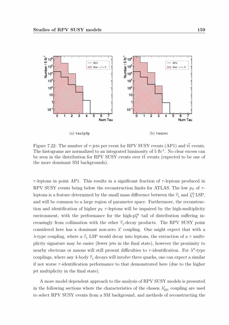
Studies of RPV SUSY models 159
Num Tau0 1 2 3 4 5 6 7
-1Nu
mbe
r / 5
fb
-110
1
10
210
310
410
510
610
Num Tau0 1 2 3 4 5 6 7
-1Nu
mbe
r / 5
fb
-110
1
10
210
310
410
510
610RPV
l + X→ttbar
(a) tau1p3p
Num Tau0 1 2 3 4 5 6 7
-1Nu
mbe
r / 5
fb
-110
1
10
210
310
410
510
610
Num Tau0 1 2 3 4 5 6 7
-1Nu
mbe
r / 5
fb
-110
1
10
210
310
410
510
610RPV
l + X→ttbar
(b) taurec
Figure 7.22: The number of τ -jets per event for RPV SUSY events (AP1) and tt events.The histograms are normalized to an integrated luminosity of 5 fb-1. No clear excess canbe seen in the distribution for RPV SUSY events over tt events (expected to be one ofthe more dominant SM backgrounds).
τ -leptons in point AP1. This results in a significant fraction of τ -leptons produced in
RPV SUSY events being below the reconstruction limits for ATLAS. The low pT of τ -
leptons is a feature determined by the small mass difference between the τ1 and χ01 LSP,
and will be common to a large region of parameter space. Furthermore, the reconstruc-
tion and identification of higher pT τ -leptons will be impaired by the high-multiplicity
environment, with the performance for the high-pvisT tail of distribution suffering in-
creasingly from collimation with the other τ1-decay products. The RPV SUSY point
considered here has a dominant non-zero λ′ coupling. One might expect that with a
λ-type coupling, where a τ1 LSP would decay into leptons, the extraction of a τ multi-
plicity signature may be easier (fewer jets in the final state), however the proximity to
nearby electrons or muons will still present difficulties to τ -identification. For λ′′-type
couplings, where any 4-body τ1 decays will involve three quarks, one can expect a similar
if not worse τ -identification performance to that demonstrated here (due to the higher
jet multiplicity in the final state).
A more model dependent approach to the analysis of RPV SUSY models is presented
in the following sections where the characteristics of the chosen λ′221 coupling are used
to select RPV SUSY events from a SM background, and methods of reconstructing the

Studies of RPV SUSY models 160
mass of the LSP are explored.
7.5 Event Selection
In order to select a sample of RPV SUSY events whilst also controlling the contribution
from Standard Model processes, a series of selection cuts are applied:
1) Cut I — ΣET selection
2) Cut II — Muon selection
3) Cut III — Z-Veto
4) Cut IV — W-Veto
5) Cut V — Jet selection
These selections take advantage of characteristics of points AP1 and AP2 to select
RPV SUSY events and reject the SM backgrounds. Each selection is defined and de-
scribed in detail in the following text. For the following analysis, the tau1p3p algorithm
was used. This choice has no impact on the motivations for any of the following selec-
tion cuts. The cuts are motivated by the dominant λ′221 coupling in points AP1 and
AP2, and aim to use the expected high jet multiplicity and also the presence of muons
to select events. Consequently they should be efficient for either the χ01 LSP or τ1 LSP
cases. Where possible the cuts have not been optimised to the specific SUSY point being
considered (other than the choice of RPV coupling). Instead the main motivation has
been the rejection of SM backgrounds.
7.5.1 Cut I — ΣET Selection
A cut on the sum of the transverse energy deposited in the calorimeter (ΣET) offers
significant rejection power against SM backgrounds which typically have lower ΣET
values. The ΣET does not include a contribution from reconstructed muons. In the
case of QCD dijet events, a ΣET cut is effective at removing lower pT events (with their
huge cross-section). Clearly such a cut becomes less effective for higher pT QCD dijets,
however the sharply falling QCD cross-section means that the rate of such events is

Studies of RPV SUSY models 161
(GeV)TEΣ0 1000 2000 3000 4000
Norm
alize
d Un
its /
20 G
eV
02468
101214161820
−310×AP1 (Excludes 17.9%)
AP2 (Excludes 16.4%)
(GeV)TEΣ0 1000 2000 3000 4000
Norm
alize
d Un
its /
20 G
eV
0
0.02
0.04
0.06
0.08
0.1 70−140 GeV)
TJ3 (p (Excludes 100%)
280−560 GeV)T
J5 (p (Excludes 78.9%)
1120−2240 GeV)T
J7 (p (Excludes 0.00157%)
(GeV)TEΣ0 1000 2000 3000 4000
Norm
alize
d Un
its /
20 G
eV
0
5
10
15
20
25
30
35
40−310×
) l + X→ttbar ( (Excludes 98.4%)
(GeV)TEΣ0 1000 2000 3000 4000
Norm
alize
d Un
its /
20 G
eV
0
10
20
30
40
50
60
70
80
−310×+2jνµ→W
(Excludes 100%)
+5jνµ→W (Excludes 94.9%)
Figure 7.23: ΣET distributions for SUSY events and selected SM backgrounds. TopLeft: RPV SUSY events, top right: QCD dijet samples (for different pT slices), bottomleft: leptonic tt events, bottom right: W → µν + n jets events (shown for n = 2 andn = 5). Each plot is normalized to unit area.
much smaller than for the lower pT dijets, and effective rejection power can be achieved
through other cuts. A cut requiring ΣET > 1000 GeV was chosen, motivated by the
ΣET distributions of SM backgrounds (in particular tt as this proves to be one of the
more significant backgrounds). Figure 7.23 demonstrates the effectiveness of such a cut
for both signal and SM background samples.
The ΣET distributions for the two RPV SUSY samples show a double peaked struc-
ture, with one population below the selection cut threshold. Figure 7.24 shows the
ΣET distributions for different SUSY production processes. One can see that the higher
ΣET population is dominated by squark and gluino production processes, with the lower

Studies of RPV SUSY models 162
population the result of the production of neutralinos and charginos. The selection cut
chosen here excludes this lower population, focusing on the dominant production of
squarks and gluinos.
(GeV)TEΣ0 1000 2000 3000 4000
Entri
es /
80 G
eV
00.20.40.60.8
11.21.41.61.8
310×
0 1000 2000 3000 400000.20.40.60.8
11.21.41.61.8
310×Production Mode
(22.2 %)g~R
q~
(20.4 %)g~L
q~
(11.7 %)R
q~R
q~
(12.8 %)R
q~L
q~
(12.4 %)L
q~L
q~
(5.77 %)g~g~
(4.09 %)±χ∼0χ∼
(2.13 %)±χ∼±χ∼
(1.13 %)l~ l~
All modes
Figure 7.24: ΣET distribution for 24000 AP2 events. The ΣET distribution for all SUSYevents is shown by the red, dashed line. The contributions from selected productionprocesses are shown separately according to the colour coding. Two populations canclearly be seen, the higher ΣET population dominated by squark and gluino production,with the lower population originating mainly from neutralino and chargino production.
7.5.2 Cut II — Muon Selection
The presence of muons in the RPV decay modes encourages a cut to select only events
with at least one candidate muon, whilst also providing strong rejection against the
QCD background. Typically, reconstructed muons in QCD events will either be mis-
reconstructed or originate from the decay of c- and b-quarks within jets. These muons
typically have low-pT and are often associated with jets, motivating the following muon
selection cuts:
• Transverse momentum, pT > 20 GeV

Studies of RPV SUSY models 163
• Calorimeter Isolation (in a cone of ∆R < 0.2), EconeT < 10 GeV
• Separation from nearest jet (for pjetT > 20 GeV), ∆Rµ−j > 0.4
As previously mentioned, boosted LSPs can result in highly collimated decay prod-
ucts, with the muon closely separated from the associated quarks in the decay. The
corresponding activity in the calorimeter around these boosted muons results in a low-
ering of the efficiency with which the reconstructed signal muons pass the calorimeter
isolation and jet separation cuts.
Figure 7.25 shows the separation of the true signal muons from the nearest recon-
structed jet in the event. It can be seen that the high-pT muons (typically originating
from the decay of a boosted LSP) are spatially closer to the nearest jet. Consequently,
the jet separation cut does not efficiently select these boosted decays. The failure to
select these decays will not necessarily have a significant effect on the subsequent mass
reconstruction, as the jets from these same decays have a higher probability of merging
into a single jet.
Num
ber /
0.0
5 / 1
0 G
eV
0
10
20
30
40
50
60
70
80
90
100
−j)µ(R∆0 0.5 1 1.5 2 2.5
(Gev
)T
True
Muo
n p
0
50
100
150
200
250
300
350
400
−j)µ(R∆0 0.5 1 1.5 2 2.5
Norm
alize
d Un
its /
0.05
0
0.02
0.04
0.06
0.08
0.1
0.12 RPV Decay Muons:
< 400 GeVT200 GeV < True p < 100 GeVT10 GeV < True p
Figure 7.25: Left: The separation of Monte Carlo muons from the nearest reconstructedjet, ∆RMC
µ−j , as a function of the true muon pT. Only signal muons from the RPV decayof the LSP are included, with ∆RMC
µ−j calculated as the separation from the nearestreconstructed jet. Only jets satisfying pT > 20 GeV and |η| < 2.5 are considered. Theevents correspond to the AP2 sample. Right: The corresponding ∆RMC
µ−j plots for twodifferent pT slices: 10 < pT < 100 GeV (red, solid line) and 200 < pT < 400 GeV (blue,dashed line). The jet separation cut is shown. Both distributions are normalized to unitarea.

Studies of RPV SUSY models 164
Figure 7.26 shows the reconstruction efficiency, as a function of the true muon pT,
for the true muons from χ01 → µqq decays. Also shown are the efficiencies when various
calorimeter isolation cuts are also applied to the reconstructed muon. It can be seen
that the calorimeter isolation cut causes a reduction in the efficiency for higher-pT muons
(particularly noticeable for the absolute isolation cut of EconeT < 10 GeV). It can be seen
that relaxing the isolation cut (by adding a component relative to the muon’s ET) can
reduce the loss in efficiency at high-pT. However, when this calorimeter isolation cut is
applied in conjunction with the jet separation cut it can be seen that the jet separation
cut dominates, and any significant benefit in signal efficiency due to the addition of a
relative component to the isolation cut is washed out (see figure 7.27). As a result,
an absolute calorimeter isolation cut of EconeT < 10 GeV was chosen (with no relative
component).
The performance in rejecting QCD events as a function of ΣET is demonstrated in
figure 7.28. No strong dependence on the ΣET can be seen, consistent with 0.013 % of
QCD events passing the selection.
(GeV)T
True Muon p0 100 200 300 400
Effic
ienc
y
00.10.20.30.40.50.60.70.80.9
1
Only Calo. Isolation Applied
Reconstructed
etcone20 < 10 GeV
T E×etcone20 < 10 GeV + 0.1
T E×etcone20 < 10 GeV + 0.3
Figure 7.26: The muon reconstruction efficiency, as a function of pT, for signal muons(only those originating from the RPV decays of the LSP). The events correspond to theAP2 sample. The efficiency is shown for cases with (i) no calorimeter isolation (trian-gles); (ii) an absolute isolation cut Econe
T < 10 GeV (yellow circles); (iii) an additionalrelative contribution of 0.1×Eµ
T (red circles) and 0.3×EµT (blue circles). One can see
that the calorimeter isolation requirements reduce the efficiency for higher pT values.This effect is reduced with the addition of a relative contribution to the isolation cut.

Studies of RPV SUSY models 165
(GeV)T
True Muon p0 50 100 150 200 250 300 350 400
Effic
ienc
y
00.10.20.30.40.50.60.70.80.9
1After Calo. Isolation & Jet Separation Cuts
etcone20 < 10 GeV
T E×etcone20 < 10 GeV + 0.3
Figure 7.27: The muon reconstruction efficiency after applying both calorimeter isolationand jet separation cuts. Two different calorimeter isolation cuts are shown (as describedin figure 7.26). See the main text for a description of the jet separation cut.
(GeV)TEΣ0 1000 2000 3000
Effic
ienc
y
0
0.05
0.1
0.15
0.2
-310×
Total Fraction Passing = 208 / 1589275 = 1.31e-04
Figure 7.28: The fraction of QCD dijet events passing the muon selection cuts as afunction of ΣET. The fraction of events passing the muon selection for the combinedQCD dijet samples is 1.31× 10⁻⁴. No significant correlation with the value of the ΣET
can be seen.

Studies of RPV SUSY models 166
7.5.3 Cut III — Z-Veto
The muon selection cuts provide significant rejection power against SM backgrounds
without genuine sources of isolated muons. However, for other SM processes further
rejection power is required. One such background is expected to arise from Z-bosons
produced in association with jets. To reject such events, a Z-veto is applied where,
for events with two reconstructed muons (at least one of which having passed the
muon selection requirements listed above), the di-muon invariant mass, mµµ, is cal-
culated. Any events with mµµ falling inside a window around the known Z-boson mass,
86 GeV < mµµ < 96 GeV, are excluded (see figure 7.29).
(GeV)µµm60 80 100 120 140
/ 1
GeV
−1Nu
mbe
r / 5
fb
0
5
10
15
20
25
30
35
40310×
+ jetsµµ →Z Excludes 71%
(GeV)µµm60 80 100 120 140
/ 1
GeV
−1Nu
mbe
r / 5
fb
10
15
20
25
30
35 AP2Excludes 5.34%
Figure 7.29: Distributions of mµµ for different physics samples. Left: Z → µµ + jets,right: RPV SUSY sample AP2. The histograms only contain events with exactly twomuons (at least one of which having passed the muon selection requirements).
7.5.4 Cut IV — W-Veto
In a similar vein, a veto is applied to reject events whereby the candidate muon (having
passed the muon selection) has originated from the decay of a W-boson. The transverse
mass, mT, is defined as:
mT =(2pµ
TpmissT (1− cos ∆φ)
) 12 (7.4)
where ∆φ is the azimuthal separation between the muon and the direction of missing
energy. mT is only calculated for events with exactly one muon passing the muon

Studies of RPV SUSY models 167
selection requirements listed in section 7.5.2. Of such events, those with mT < 90 GeV
are rejected (see figure 7.30). Events with a greater number of candidate muons pass the
veto. This cut provides rejection against backgrounds both from W-bosons produced
in association with jets, and also tt events (where tt background remaining after the
previous muon selection cuts can be expected to be dominated by events where a t-
quark decays through the muon channel, t → bW → bµν). Unfortunately this is at the
expense of a significant fraction of the RPV SUSY events. In order to control the large
tt cross-section, a hard cut is needed.
(GeV)Tm0 100 200 300 400
/ 5
GeV
−1Nu
mbe
r / 5
fb
0
0.05
0.1
0.15
0.2
0.25
0.3
0.35
0.4
610× + jetsνµ →W
Excludes 89.8%
(GeV)Tm0 100 200 300 400
/ 5
GeV
−1Nu
mbe
r / 5
fb
0
5
10
15
20
25
30
35
40
310×) l + X→ttbar (
Excludes 80%
(GeV)Tm0 100 200 300 400
/ 5
GeV
−1Nu
mbe
r / 5
fb
020406080
100120140160180200 AP2
Excludes 42.8%
Figure 7.30: Distributions of mT for different physics samples. Top left: W → µν + jets,top right: tt and bottom: RPV SUSY sample AP2. Only events with exactly one muonpassing the muon selection requirements, listed in section 7.5.2, are considered.

Studies of RPV SUSY models 168
7.5.5 Cut V — Jet Selection
The jet selection cuts are motivated by the details of the RPV coupling being inves-
tigated. For the dominant λ′ coupling being studied here, one can expect each SUSY
cascade decay to end in a LSP-decay producing two jets (originating from the quarks in
the decay). With squark and gluino production being dominant, one can expect further
jet production at the head of each decay chain. It is therefore reasonable to expect at
least six jets in a given SUSY event. Figure 7.31 shows the distribution for the number
of jets per event for the SUSY AP2 sample. The merging of overlapping jets can lower
the number of jets actually seen (this is particularly significant in the case where the
LSP is highly boosted, resulting in collimated decay products). Such merged jets are
not useful for the purpose of reconstructing the mass of the LSP in this analysis. The
decay of squarks/gluinos at the start of each SUSY decay chain will typically produce
two hard jets per event, motivating a cut on the pT of the two hardest jets in the event.
In summary, the following jet selection cuts are applied:
• Transverse momentum of the hardest jet, p(0)T > 200 GeV
• Transverse momentum of the second hardest jet, p(1)T > 100 GeV
• The number of candidate jets (with pT > 20 GeV and |η| < 2.5), Njet ≥ 6
jetN0 5 10 15 20
-1Ev
ents
/ 5
fb
0
0.5
1
1.5
2
2.5
3
3.5
4
310×
Mean = 6.98 RMS = 2.11
Figure 7.31: The number of jets per event for AP2. Only jets satisfying pT > 20 GeVand |η| < 2.5 are considered.

Studies of RPV SUSY models 169
7.5.6 Event selection performance and background rejection
Tables 7.6, 7.7 and 7.8 give a summary of the event selection performance for both
RPV SUSY and SM background Monte Carlo samples. The expected number of events
after the event selection is shown for each sample, normalized to an integrated luminosity
(L) of 5 fb-1. Due to the large cross-sections for some of the SM backgrounds, the avail-
able statistics were not sufficient in all samples. Consequently, where the cuts remove
all the events in a sample, the 90 % confidence limit is quoted. For the two RPV SUSY
samples considered, the expected number of events after event selection are ∼ 3000–3400
for L = 5 fb-1. Of the SM backgrounds, the dominant observed contribution comes from
tt events (∼ 480), with a further significant contribution from W → µν + jets (∼ 250).
For the QCD samples with adequate statistics (J6 and J7), there is no significant
contribution. However, for the lower-pT QCD samples (J3, J4 and J5), the available
statistics do not allow the precise contributions to be established. The Poisson confidence
limits show that the contribution from QCD cannot be discounted initially (however, it
can be seen that one runs out of statistics before fully exploring the rejection power of
the muon, W -veto and jet cuts).
For the W → µν + n jets samples, the dominant contribution comes from those
events with higher numbers of additional jets (n = 5). For the samples with a lower
numbers of jets (n = 2, 3), the results are statistically limited before the full rejection
power of the jet selection cuts is applied. The contributions from these samples are
neglected as the rejection power of the jet selection cut will increase with decreasing
values of n, giving small contributions compared to the n = 5 case.
Whilst the small sample statistics for W → τν + jets result in significant confidence
limits, the contribution from W → τν + jets is also expected to be negligible. In the case
of W → τν + jets, one can argue that the expected rate of events passing the selection
cuts would be lower than that for W → µν + jets as the branching ratio for τ → µνµντ
and the softer pT spectrum of the resulting muon would both reduce the efficiency of
W → τν + jets events passing selection with respect to W → µν + jets events.
For the other backgrounds considered, Z → µµ + jets contributes ∼ 50 events (an
order of magnitude lower than the more dominant backgrounds already discussed), and
the contributions from Z → ττ + jets are seen to be a further order of magnitude smaller.
For both the Z → µµ + jets and Z → ττ + jets sets of samples, the limits placed on the
contributions where n = 2, 3 are small and are neglected.

Studies of RPV SUSY models 170
Sam
ple
Tot
alC
uts
L=
5fb
−1
Eve
nts
Cut
IC
ut
IIC
ut
III
Cut
IVC
ut
VSUSY
AP
124
125
1981
383
0081
1748
9438
0829
99(8
2.1%
)(3
4.4%
)(3
3.6%
)(2
0.3%
)(1
5.8%
)
AP
224
000
2005
580
4578
9450
1139
2634
35(8
3.6%
)(3
3.5%
)(3
2.9%
)(2
0.9%
)(1
6.4%
)
tt
tt→
``/h
`43
6886
6789
1167
1156
273
9347
9(1
.55%
)(0
.267
%)
(0.2
65%
)(0
.062
5%)
(0.0
213%
)
tt→
hh
4566
016
232
20
0<
96
(3.5
5%)
(0.0
0438
%)
(0.0
0438
%)
(0%
)(0
%)
(90%
CL)
QCD
J334
4050
890
00
0<
2.06
0×
105
(0.0
259%
)(0
%)
(0%
)(0
%)
(0%
)(9
0%C
L)
J437
7400
1434
00
00
<96
66
(0.3
8%)
(0%
)(0
%)
(0%
)(0
%)
(90%
CL)
J528
4450
5989
311
110
0<
505
(21.
1%)
(0.0
0387
%)
(0.0
0387
%)
(0%
)(0
%)
(90%
CL)
J639
1800
3910
3237
371
14.
4(9
9.8%
)(0
.009
44%
)(0
.009
44%
)(0
.000
255%
)(0
.000
255%
)
J719
1575
1915
7233
336
10.
1(1
00%
)(0
.017
2%)
(0.0
172%
)(0
.003
13%
)(0
.000
522%
)
Tab
le7.
6:E
vent
sele
ctio
ncu
tflow
:SU
SY
,tt
and
QC
D.

Studies of RPV SUSY models 171
Sam
ple
Tot
alC
uts
L=
5fb
−1
Eve
nts
Cut
IC
ut
IIC
ut
III
Cut
IVC
ut
V
W→µν+njets
W→
µν
+2j
4945
020
1717
30
<15
7
(0.0
404%
)(0
.034
4%)
(0.0
344%
)(0
.006
07%
)(0
%)
(90%
CL)
W→
µν
+3j
4700
010
664
6319
0<
49
(0.2
26%
)(0
.136
%)
(0.1
34%
)(0
.040
4%)
(0%
)(9
0%C
L)
W→
µν
+4j
3195
437
024
123
945
19.
1(1
.16%
)(0
.754
%)
(0.7
48%
)(0
.141
%)
(0.0
0313
%)
W→
µν
+5j
9750
499
335
334
7123
245
(5.1
2%)
(3.4
4%)
(3.4
3%)
(0.7
28%
)(0
.236
%)
W→τν+njets
W→
τν
+2j
6000
20
00
0<
280
(0.0
333%
)(0
%)
(0%
)(0
%)
(0%
)(9
0%C
L)
W→
τν
+3j
1500
41
10
0<
356
(0.2
67%
)(0
.066
7%)
(0.0
667%
)(0
%)
(0%
)(9
0%C
L)
W→
τν
+4j
2900
6010
100
0<
56
(2.0
7%)
(0.3
45%
)(0
.345
%)
(0%
)(0
%)
(90%
CL)
W→
τν
+5j
2000
142
2424
00
<31
(7.1
%)
(1.2
%)
(1.2
%)
(0%
)(0
%)
(90%
CL)
Tab
le7.
7:E
vent
sele
ctio
ncu
tflow
:W→
µν
+n
jets
and
W→
τν
+n
jets
.

Studies of RPV SUSY models 172
Sam
ple
Tot
alC
uts
L=
5fb
−1
Eve
nts
Cut
IC
ut
IIC
ut
III
Cut
IVC
ut
V
Z→µµ+njets
Z→
µµ
+2j
4765
015
114
20
<15
(0.0
315%
)(0
.023
1%)
(0.0
0839
%)
(0.0
042%
)(0
%)
(90%
CL)
Z→
µµ
+3j
4700
013
811
561
360
<5
(0.2
94%
)(0
.245
%)
(0.1
3%)
(0.0
766%
)(0
%)
(90%
CL)
Z→
µµ
+4j
4250
054
948
223
612
14
2.7
(1.2
9%)
(1.1
3%)
(0.5
55%
)(0
.285
%)
(0.0
0941
%)
Z→
µµ
+5j
1120
060
551
525
414
553
49.5
(5.4
%)
(4.6
%)
(2.2
7%)
(1.2
9%)
(0.4
73%
)
Z→ττ+njets
Z→
ττ
+2j
4235
028
1010
20
<7
(0.0
661%
)(0
.023
6%)
(0.0
236%
)(0
.004
72%
)(0
%)
(90%
CL)
Z→
ττ
+3j
3500
123
30
0<
28
(0.3
43%
)(0
.085
7%)
(0.0
857%
)(0
%)
(0%
)(9
0%C
L)
Z→
ττ
+4j
3130
062
515
915
97
0<
1
(2%
)(0
.508
%)
(0.5
08%
)(0
.022
4%)
(0%
)(9
0%C
L)
Z→
ττ
+5j
9250
711
180
180
114
2.1
(7.6
9%)
(1.9
5%)
(1.9
5%)
(0.1
19%
)(0
.043
2%)
Tab
le7.
8:E
vent
sele
ctio
ncu
tflow
:Z→
µµ
+n
jets
and
Z→
ττ
+n
jets
.

Studies of RPV SUSY models 173
Revisiting the QCD background, table 7.9 shows the rejection of QCD events after
the application of only the muon selection cuts and the W/Z-vetoes (cuts II, III and IV).
Combining the events from the different QCD samples, one can see that out of a total
of 1,589,275 events, 208 pass the muon cut (0.013 %) and only 8 events (0.0005 %) pass
both the muon selection and W/Z-vetoes. The rejection power from these cuts alone
suggest that there is further significant rejection power that is not used by the limited
simulated data statistics. This implies that the selection cuts offer further rejection
against the low-pT QCD background than the confidence limits in table 7.6 suggest
(provided there aren’t strong correlations between the combined muon selection cut and
W-veto, and the ΣET selection cut).
Figure 7.28 shows no significant correlation between the efficiency with which QCD
events pass the muon cuts with the ΣET of the event. The very small statistics available
for events going on to also pass the W-veto do not allow a full test of the correlation of
this cut to be established with the ΣET cut. However it is reasonable to assume that
the higher pT QCD events would be more likely to pass the mT cut (a non-zero pmissT is
needed to generate a significant mT value, with larger pmissT values expected in the QCD
events at higher pT scales). Consequently, the assumption that the rejection power of
the combined muon selection and W-veto is uncorrelated with the ΣET of the event will
be conservative for the low-pT QCD events for which there are limited statistics (e.g.
samples J3 and J4). To factor this effect into the event selection performance for the
J3, J4 and J5 QCD samples, the confidence levels are adjusted in accordance with the
expected remaining rejection power of the muon selection and W-veto cuts (applying
a cut efficiency of 0.0005 % to the events remaining after the output of the ΣET cut
for samples J3 and J4, and a cut efficiency of 3.8 % to the events remaining after the
W-veto cut for sample J5). It should be noted that this does not take into account
the further effect of the jet selection (cut V), which should provide some extra rejection
power (although this is expected to show some significant correlation with the ΣET cut).
The resulting background contributions for the QCD samples are summarised in table
7.10. It can be seen that the background contribution from QCD is at a controlled level
even before the jet selection is considered for samples J3, J4 and J5.
The contributions from the different sources of background are combined to give
an overall measure of the expected SM background. The probability density functions
(PDFs) for each sample are combined to give an overall PDF for the number of SM events
passing the event selection. Table 7.11 shows the overall numbers of signal and back-
ground expected in 5 fb-1 of data (the full statistical analysis is described in appendix B).

Studies of RPV SUSY models 174
The combined SM background is predicted to be 986 +119−121 (stat)± 102 (xsec). The event
selection process indicates that RPV SUSY events can be selected from SM events with
a signal to background ratio (S/B) of 3.04± 0.37 (stat) +0.27−0.33 (xsec) for point AP1, and
3.48± 0.43 (stat) +0.31−0.37 (xsec) for point AP2. The errors on the cross-sections, (xsec),
are assumed to be correlated.
SampleTotal Cuts
L = 5fb−1
Events Cut II Cut III Cut IV
QC
D
J3 34405055 55 0 < 2.060× 10⁵
(0.016%) (0.016%) (0%) (90% CL)
J4 37740040 40 0 < 9666
(0.0106%) (0.0106%) (0%) (90% CL)
J5 28445043 43 1
220(0.0151%) (0.0151%) (0.000352%)
J6 39180037 37 1
4.4(0.00944%) (0.00944%) (0.000255%)
J7 19157533 33 6
0.9(0.0172%) (0.0172%) (0.00313%)
Table 7.9: Event selection cut flow for cuts II, III and IV only: QCD.
Sample Events in L = 5 fb-1
J3 < 91.7
J4 < 69.3
J5 < 213
J6 4.4± 4.4
J7 0.1± 0.1
Table 7.10: The background contribution from QCD after event selection for L = 5 fb-1.The confidence limits are adjusted to incorporate the expected redundant rejection powerfrom cuts II, III and IV.

Studies of RPV SUSY models 175
Sample Events in L = 5 fb-1 S/B
SM 986 +119−121± 102 —
AP1 2999± 49± 600 3.04± 0.37 +0.27−0.33
AP2 3435± 55± 687 3.48± 0.43 +0.31−0.37
Table 7.11: A summary of numbers of SUSY and SM events after the event selec-tion process for both SUSY points AP1 and AP2. Also shown is the S/B ratio whereSUSY events are considered as signal S, and the SM events are considered as back-ground B. The statistical and cross-section errors are quoted separately in the formA±σstat.±σx−section. The errors in the SM and SUSY cross-sections are taken to becorrelated in calculating S/B.
7.6 Triggers
The ability to trigger on signal events is clearly essential to any prospects of observing
RPV SUSY in ATLAS. For the RPV coupling studied here, with high jet multiplicities
and muons in the final state, the topology of SUSY events implies that multi-jet and
muon triggers will be useful in extracting a signal from the detector.
From the standard ATLAS CSC trigger menu8, the following trigger items were in-
vestigated:
1) mu20i — a single muon trigger with a threshold of pT > 20 GeV
2) 3jet65 — a multi-jet trigger, requiring three jets above a 65 GeV threshold
3) 4jet50 — a multi-jet trigger, requiring four jets above a 50 GeV threshold
The mu20i trigger is expected to be unprescaled when running at a luminosity of
1033 cm-2s-1 (as planned for the early running period) and provides efficient selection
of signal events. By also considering a combination of a muon and multi-jet trigger
one can enhance the trigger efficiency. The available multi-jet options in the CSC trigger
menu are 3jet65 and 4jet50. However the final trigger menu for running at 1033 cm-2s-1
is not finalised and the trigger thresholds may be higher than those presented here ([80]
suggests thresholds of 110 GeV and 165 GeV for the 3- and 4-jet triggers). Table 7.12
shows the efficiency with which RPV SUSY events are triggered by the above triggers
8The trigger menu run by default during the Monte Carlo production for the ATLAS CSC exercise.

Studies of RPV SUSY models 176
(and the “OR” combination of the mu20i trigger with each of the 3jet65 and 4jet50
triggers). Also shown are the efficiencies for the subset of events that pass the event
selection cuts. It can be seen that a combination of muon and multi-jet triggers selects
92–95 % of all RPV SUSY events and > 99 % of those that pass the event selection, thus
providing efficient performance for collecting signal events. Without considering multi-
jet triggers, the mu20i trigger selects 88 % of those events passing the event selection. As
an indication of how the trigger selection efficiency is sensitive to the transverse energy
threshold of the multijet trigger, figure 7.32 shows the efficiency with which events pass
either the mu20i trigger or have 3 (or 4) reconstructed jets above a varying threshold in
transverse energy. Whilst reconstructed jets do not exactly correspond to the jet trigger
objects that are used to form a trigger decision, they can provide a good approximation.
It can be seen that the 3- or 4-jet triggers should offer significant additional efficiency
(above the baseline mu20i trigger) for a significant range of trigger thresholds.
Trigger
Efficiency Efficiency
(All Events) (Events Passing ES)
AP1 AP2 AP1 AP2
mu20i 58.4% 52.0% 88.4% 87.5%
3jet65 87.9% 90.5% 97.8% 98.6%
4jet50 82.1% 85.4% 94.6% 95.9%
mu20i | 3jet65 94.6% 95.2% 99.7% 99.8%
mu20i | 4jet50 92.2% 92.9% 99.3% 99.4%
Table 7.12: A table showing the efficiency with which RPV SUSY events for points AP1and AP2 pass selected triggers. The percentage of events passing the triggers are shownboth for all events in the samples, and for the subset of events that also pass the eventselection (ES) cuts.

Studies of RPV SUSY models 177
(GeV)TThreshold E0 100 200 300 400 500
Effic
ienc
y (%
)
0
20
40
60
80
100
(Pre ES)T3 Jets above E (Pre ES)T4 Jets above E (Post ES)T3 Jets above E (Post ES)T4 Jets above E
(a) AP1
(GeV)TThreshold E0 100 200 300 400 500
Effic
ienc
y (%
)
0
20
40
60
80
100
(Pre ES)T3 Jets above E (Pre ES)T4 Jets above E (Post ES)T3 Jets above E (Post ES)T4 Jets above E
(b) AP2
Figure 7.32: The percentage of RPV SUSY events for point (a) AP1 and (b) AP2 thateither pass the mu20i trigger or have at least 3 (or 4) reconstructed jets with transverseenergies above a given threshold (ET). The efficiency is shown separately for eventsbefore (blue lines) and after the event selection (red lines).

Studies of RPV SUSY models 178
7.7 Measuring the χ01 LSP mass in point AP2
The focus of this analysis now moves on to point AP2, looking in particular at the
reconstruction of the mass of χ01 LSP. Having applied a series of event selection cuts to
reduce the SM background (as described in section 7.5.6), the surviving events undergo a
mass reconstruction process, aimed at determining the χ01 mass through the observation
of χ01 → µqq decays. The SUSY signal selected by the event selection process contains a
variety of different decay chains. However almost all events will include two χ01s, with the
muon selection cuts picking events where at least one χ01 decays through the χ0
1 → µqq
channel.
7.7.1 Mass combinations
In order to reconstruct the χ01 mass (Meχ0
1), a method based on calculating the invariant
mass for combinations of a muon and two jets is employed. The challenge of finding
the correct combinations in a high-multiplicity environment leads to a significant combi-
natorial background from SUSY events in addition to the remaining SM contributions.
To counter the combinatorial background the following procedure is used. An isolated
muon is used to seed the combination, forming an invariant mass with two associated
jets. Cuts are applied to the transverse momentum of the first associated jet, pj1T , and
second associated jet, pj2T , while the associated jets are restricted to lie in a reconstruction
cone centred on the seed muon (with cone-size ∆Rµjj). The cut values are summarised
below.
1) A seed muon with pµT > 20 GeV (satisfying the isolation and jet separation cuts
described in section 7.5.2)
2) An associated jet with 20 GeV < pj1T < 250 GeV, |η| < 2.5 and ∆Rµjj < 1.5
3) A second associated jet with 20 GeV < pj2T < 150 GeV, |η| < 2.5 and ∆Rµjj < 1.5
Figure 7.10(b) shows the pT distributions of the decay quarks, motivating the above
cuts on jet-pT. By only considering jets within a cone of ∆Rµjj < 1.5 from the seed
muon, one can exploit the collimation of the χ01 decay products. In its extreme, this
collimation will have a detrimental affect on the reconstruction of χ01 decays as it will
lead to the merging of the two decay jets and will also impact on the muon’s isolation

Studies of RPV SUSY models 179
(as demonstrated in figures 7.25 and 7.27). However, for moderate boosts the decay
products will tend to be closely associated. The jets and muons that form incorrect
combinations will not be expected to show any significant correlation in their position
so the cut on ∆Rµjj acts to reduce the SUSY combinatorial background (and also the
SM background).
Since each seed muon can only be associated with one χ01 decay, for seed muons
forming multiple combinations, each of the resulting Mµjj values are weighted by the
reciprocal of the total number of combinations, 1/Ncom. A cut requiring that Ncom ≤ 3
is applied such that seed muons forming higher numbers of combinations are rejected
(in such cases, for any correct combinations that are found, there will be at least three
incorrect combinations contributing to the combinatorial background).
Figure 7.33 shows the Mµjj distribution. A mass-peak can be seen above a back-
ground distribution. The dominant background originates from the SUSY combinatorial
background, with a smaller SM contribution. Monte Carlo truth information is used to
separate the signal peak from the SUSY combinatorial background in a process where
the true quarks and muons from signal χ01 → µqq decays are matched to the recon-
structed muons and jets that make a combination. The magnitude of this combinatoric
background may itself be considered a signature of some new physics. This is because
the λ′221 RPV coupling results in decays to muons, so one can expect to see an excess of
muons with respect to electrons in SUSY events. One would expect that the combina-
toric background for Mµjj combinations to be larger than for a corresponding analysis
where electrons were considered instead of muons (once any differences in electron and
muon reconstruction efficiencies were considered). In the SM alone, the production of
muons and electrons would be expected to occur at approximately the same rate. This
aspect of the RPV phenomenology has not been exploited in the analysis presented here.
7.7.2 Combinatoric background estimation
As shown in figure 7.33, the Mµjj distribution shows a mass-peak above a broader back-
ground distribution. In establishing the presence of a signal mass-peak, it is important
to estimate the shape of the background distribution, a process made more difficult by
the peak in the background shape lying relatively close to the signal peak. The back-
ground shape is not known, and whilst one may attempt to fit an arbitrary functional
form to the background, it would be more desirable to establish this shape from data.
A data-driven approach to estimating the background shape is presented below.

Studies of RPV SUSY models 180
(GeV)jjµM0 100 200 300 400 500 600
/ 10
GeV
-1Nu
mbe
r / 5
fb
0
50
100
150
200
250
300
0 100 200 300 400 500 6000
50
100
150
200
250
300SUSY SignalSUSY Combin. BGSM BG
01
χ∼
Figure 7.33: A stacked plot showing the Mµjj distributions for RPV SUSY point AP2,where (i) SUSY signal, (ii) SUSY combinatorial background and (iii) SM backgroundare shown separately. Only events passing the event selection are considered.
For each of the n events passing the event selection, “manufactured” events are
formed by merging the muons from one event with the jets from another event. In total,
n(n−1) manufactured events are formed (see figure 7.34). By construction, the position
of the muons in these events will not be correlated with the jets, unlike those found in
events with true χ01 decays. By forming the Mµjj distribution from the manufactured
events, an estimate of the background distribution is obtained. The background estimate
is shown in figure 7.35, weighted to correspond to the same total number of events.
7.7.3 Systematic Errors
The uncertainty in the precise shape of the background distribution will be a source of
systematic error on the reconstruction of the χ01 mass. In order to test the sensitivity of
the measurement to the background model used to subtract the background shape from
the Mµjj distribution, a second approach to modelling this background was tested. This
is demonstrated in figure 7.36, where a function of the form:
f (x) = kxa (1− x)b (7.5)
is used to fit the background shape. In this model x is defined to be a linear function of
Mµjj such that f (x) = 0 at appropriate values of Mµjj (a low cut-off determined by the

Studies of RPV SUSY models 181
η-3 -2 -1 0 1 2 3
φ
-3
-2
-1
0
1
2
3
η-3 -2 -1 0 1 2 3
φ
-3
-2
-1
0
1
2
3
η-3 -2 -1 0 1 2 3
φ
-3
-2
-1
0
1
2
3
η-3 -2 -1 0 1 2 3
φ
-3
-2
-1
0
1
2
3
η-3 -2 -1 0 1 2 3
φ
-3
-2
-1
0
1
2
3
η-3 -2 -1 0 1 2 3
φ
-3
-2
-1
0
1
2
3
η-3 -2 -1 0 1 2 3
φ
-3
-2
-1
0
1
2
3
η-3 -2 -1 0 1 2 3
φ
-3
-2
-1
0
1
2
3
η-3 -2 -1 0 1 2 3
φ
-3
-2
-1
0
1
2
3
η-3 -2 -1 0 1 2 3
φ
-3
-2
-1
0
1
2
3
η-3 -2 -1 0 1 2 3
φ
-3
-2
-1
0
1
2
3
η-3 -2 -1 0 1 2 3
φ
-3
-2
-1
0
1
2
3
η-3 -2 -1 0 1 2 3
φ
-3
-2
-1
0
1
2
3
η-3 -2 -1 0 1 2 3
φ
-3
-2
-1
0
1
2
3
η-3 -2 -1 0 1 2 3
φ
-3
-2
-1
0
1
2
3
η-3 -2 -1 0 1 2 3
φ
-3
-2
-1
0
1
2
3
η-3 -2 -1 0 1 2 3
φ
-3
-2
-1
0
1
2
3
η-3 -2 -1 0 1 2 3
φ
-3
-2
-1
0
1
2
3
Other Events
"Manufactured" Events
Selected Event
Jets
Muons
Figure 7.34: A schematic diagram describing the merging of uncorrelated muons andjets from different events in order to create a set of “manufactured” events. Thesemanufactured events are studied in order to model the background distribution.

Studies of RPV SUSY models 182
(GeV)jjµM0 100 200 300 400 500 600
/ 10
GeV
-1Nu
mbe
r / 5
fb
0
50
100
150
200
250
300
0 100 200 300 400 500 6000
50
100
150
200
250
300SUSY SignalSUSY Combin. BGSM BGBackground estimate
01
χ∼
(GeV)jjµM0 100 200 300 400 500 600
/ 10
GeV
-1Nu
mbe
r / 5
fb
0
50
100
150
200
01
χ∼Gauss. Fit
1.3 GeV±Mean = 158.5 1.8 GeV±Sigma = 15.61
Figure 7.35: Left: A stacked plot showing the Mµjj distribution for RPV SUSY pointAP2 (as figure 7.33). The estimated background distribution (red line) is also shown(normalized to the same number of events). Right: The Mµjj distribution after back-ground subtraction. The peak is fitted with a Gaussian.
kinematic constraints of the combination cuts, and a high cut-off where the Mµjj can
safely be assumed to be negligible). The motivation for this functional-fit method is to
use the rising and falling tails of the distribution (where no signal events are expected)
to infer the full distribution beneath the peak in an independent way to that presented
in section 7.7.2. This functional-fit model is therefore reliant on understanding where
the tails of the signal distribution lie (as it is important not to be biased by the presence
of signal when fitting the background). Where the peak can clearly be seen above the
background one can be confident of selecting signal free regions. However this may not
always be the case.
Figure 7.36 demonstrates that the functional-fit provides a good description of the
background, allowing a clear mass-peak to be seen. A comparison with the background
subtraction by the independent data-driven method demonstrated in figure 7.35 gives
a measure of the sensitivity of the χ01 mass measurement to the understanding of the
underlying background distribution. Table 7.13 shows the value of the reconstructed χ01
mass for these two methods and it can be seen that the Meχ01
measurement is robust to
the choice of background model. However the predicted number of background events is
susceptible to a larger systematic error which will have an implication on the significance
of the observed peak in data. With the data-driven method, the estimated number of
background events inside a mass window of 120 GeV < Mµjj < 200 GeV, is B = 675

Studies of RPV SUSY models 183
(GeV)jjµM0 100 200 300 400 500 600
/ 10
GeV
-1Nu
mbe
r / 5
fb
0
50
100
150
200
250
300
0 100 200 300 400 500 6000
50
100
150
200
250
300SUSY SignalSUSY Combin. BGSM BG
fitb(1-x)ax
01
χ∼
(GeV)jjµM0 100 200 300 400 500 600
/ 10
GeV
-1Nu
mbe
r / 5
fb
020406080
100120140160180 0
1χ∼
Gauss. Fit
1.1 GeV±Mean = 158.7 1.2 GeV±Sigma = 9.245
Figure 7.36: Left: A stacked plot showing the Mµjj distributions for RPV SUSY pointAP2 (as figure 7.33). The rising and falling tails of the distribution are used to fit afunction of the form kxa(1 − x)b as a further estimate of the background distribution(blue line). Right: The Mµjj distribution after subtraction of this function. The peakis fitted with a Gaussian.
events. The functional-fit method gives B = 932. The difference in the two values
gives a measure of the systematic error associated with the definition of the background
model. Consequently a systematic error of 30 % is assigned to the value of B calculated
from the background model.
It should be noted that the SM distribution is given by the simulated events passing
the event selection. As discussed in section 7.5.6 and appendix B, the contribution from
QCD is limited by statistics, and is not accounted for in the SM distribution shown here.
The total number of SM events passing the event selection is predicted by the statistical
analysis (summarised in table B.3) to be 986 +119−121± 102. After event selection, no events
are available for the J3, J4 and J5 QCD samples, so no contributions could be made to
the Mµjj distribution shown in figure 7.33. The total (luminosity weighted) number of
SM events included in the Mµjj distribution shown is 792 events. This is ∼ 20 % lower
than the 986 +119−121± 102 calculated in appendix B. The impact of this discrepancy on the
measurement of Meχ01
will be a second order effect as an increase in the SM contribution
will also be reflected in the the estimation of the combinatoric background and subtracted
accordingly. The impact on the discovery reach will be larger as the relative number
of signal to background combinations below the Mµjj peak will be affected. However
since the systematic error on the background shape is large and the SUSY combinatoric
background dominates the SM contribution, this effect is not considered to be significant

Studies of RPV SUSY models 184
Bgnd. Model χ01 Mass Peak Peak
∆Rµjj α β Ncom (GeV) ST /BT ST /√
BT
1.5 ✓ ✗ ≤ 3 158.5± 1.3 0.47 14.1
1.5 ✗ ✓ ≤ 3 158.7± 1.1 0.47 14.1
2.0 ✓ ✗ ≤ 3 158.6± 1.6 0.36 10.9
2.5 ✓ ✗ ≤ 3 157.3± 2.1 0.30 7.54
1.5 ✓ ✗ = 1 157.8± 1.3 0.64 14.5
1.5 ✓ ✗ Any 158.2± 1.3 0.42 13.6
2.5 ✓ ✗ = 1 162.0± 5.0 0.47 6.7
2.5 ✓ ✗ Any 159.6± 2.5 0.20 7.4
Table 7.13: A summary table showing the reconstructed χ01 mass for different recon-
struction parameters. Background model “α” corresponds to the data-driven approach,whilst model “β” corresponds to the functional-fit approach. Also shown are the ST/BT
and ST/√BT values calculated in a window of 120 GeV < Mµjj < 200 GeV using the
Monte Carlo truth.
when compared to the other sources of error.
The sensitivity of the background estimate to the value of ∆Rµjj is demonstrated in
figure 7.37 (for cone sizes of ∆Rµjj = 2.0 and ∆Rµjj = 2.5). The impact on the value
of the reconstructed mass for different cone sizes is shown in table 7.13. The method is
robust with respect to the choice of cone size, with the reconstructed χ01 mass not signif-
icantly affected by changes to ∆Rµjj. Defining a window of 120 GeV < Mµjj < 200 GeV
around the mass-peak, the values of ST/BT and ST/√BT are also shown in table 7.13 for
varying ∆Rµjj values. Here the total weight of signal combinations (ST ) and the weight
of background combinations (BT ) are calculated from the Monte Carlo truth informa-
tion. These true numbers are quoted in order to provide a measure of the performance
of the mass combination procedure and should not be confused with any measure of
discovery potential. It can be seen that the relative background contribution increases
with increased ∆Rµjj, with the smaller choice of ∆Rµjj = 1.5 giving the best ratio of
signal to background in the peak. Whilst the reconstructed mass is not found to be
sensitive to the cone size, the signal significance is increased by considering a smaller
cone.

Studies of RPV SUSY models 185
(GeV)jjµM0 100 200 300 400 500 600
/ 10
GeV
-1Nu
mbe
r / 5
fb
0
50
100
150
200
250
0 100 200 300 400 500 6000
50
100
150
200
250 SUSY SignalSUSY Combin. BGSM BGBackground estimate
01
χ∼
(a) ∆Rµjj = 2.0
(GeV)jjµM0 100 200 300 400 500 600
/ 10
GeV
-1Nu
mbe
r / 5
fb
020406080
100120140160180
0 100 200 300 400 500 600020406080
100120140160180
SUSY SignalSUSY Combin. BGSM BGBackground estimate
01
χ∼
(b) ∆Rµjj = 2.5
Figure 7.37: Mµjj distributions (as described in figure 7.35) for varying ∆Rµjj values.
Since the reconstruction of Meχ01
involves the combination of two jets, one can expect
that the error in establishing the jet-energy scale (JES) will be one of the more significant
systematic errors in making this measurement (and should dominate over the uncertainty
in the muon measurement). The sensitivity of the Meχ01
measurement to the JES was
investigated in a procedure involving the rescaling of the jet 4-momenta in steps of
2.5 % between −7.5 % and 7.5 %. Neither the event selection, nor the ΣET value were
changed during the rescaling process. The impact of a systematic offset in the JES on
the measured value of Meχ01is shown in figure 7.38. It can be seen that Meχ0
1varies linearly
with the JES, with a resulting systematic error of 1.3 GeV for every 1.0 % uncertainty
in the JES.
7.8 Discovery Reach
The analysis presented here has demonstrated a method for directly reconstructing the
mass of the unstable χ01 LSP as occurring in point AP2. As an indication of the discovery
potential of such a signature in ATLAS, the significance of the signal is now discussed. It
should be noted that when considering RPV SUSY models there is a very large parameter
space to explore, over which the SUSY mass scale and production cross-section can vary.
These variations will have an effect on the discovery potential as a function of the point

Studies of RPV SUSY models 186
JES Offset (%)-10 -5 0 5 10
(GeV
)jjµ
Peak
M
150
155
160
165
170 JES sensitivity = 1.3 GeV / 1.0 %
= 157.9 GeV01
χM
Figure 7.38: The sensitivity of the χ01 mass measurement to the JES.
in SUSY parameter space.
Figure 7.39 shows the simulated Mµjj distribution (normalized to L = 5 fb-1) with
an estimate of the background as determined by the data-driven method. The dominant
error on the background is the systematic error associated with the background shape
(∼ 30 %). Counting combinations inside a window of 120 GeV < Mµjj < 200 GeV, the
total weighted number is T = 1297± 42 with the data-driven background model pre-
dicting a background contribution of B = 675± 202. The error on B is dominated by
the systematic error in the background model, whilst the statistical error is very small.
Defining S = T−B, the significance of the signal peak is given by S/√B = 24.0± 11.5.
Here the systematic error (48 %) dominates the statistical error (7 %). Extrapolating
this result to lower numbers of events suggests that a significance of S/√B = 5.0± 2.8
could be achieved with an integrated luminosity of L = 0.2 fb-1. The statistical error of
28 % is still very much less than the systematic error of 48 %. This suggests that the
observation of such a signal would be possible in early data. An integrated luminosity of
L = 6 fb-1 is predicted during running in 2009 [81] (at a peak luminosity of 1033 cm-2s-1).
The above method provides a simple measure of the signal significance. In an analysis
using real ATLAS data, it would be important to carefully consider the choice and width
of the window in which the peak is observed when considering a possible signal. The cuts
presented here have not been strongly optimised and it is important that cuts are not
over-optimised in order to enhance the signal peak. More detailed statistical methods
could take into account the shape of the signal peak and background distributions in

Studies of RPV SUSY models 187
(GeV)jjµM0 100 200 300 400 500 600
/ 10
GeV
-1Nu
mbe
r / 5
fb
0
50
100
150
200
250
300 Simulated DataBackground EstimateSystematic Error Band
Figure 7.39: The Mµjj distribution for point AP2 with the data-driven background es-timate and the associated systematic error band. ∆Rµjj = 1.5 and Ncom ≤ 3. The sys-tematic error band shows a 30 % uncertainty. A window of 120 GeV < Mµjj < 200 GeVis applied around the peak.
determining the signal significance. However, in the context of the analysis presented
here, and when considering a single point in a large parameter space, the benefits of using
more advanced methods are limited. Clearly uncertainties in the delivered luminosity,
the Monte Carlo cross-sections and trigger efficiencies will determine the exact timescale
of discovery should such a RPV SUSY model exist, not forgetting the possible variation
in SUSY mass-scale and production cross-section. However, should such a model exist
in nature, the reconstruction of the χ01 mass in RPV SUSY models with decays of the
form χ01 → µqq can be expected in the first years of running.
7.9 Measuring the τ1 LSP mass in point AP1
Having discussed the measurement of the χ01 LSP mass for point AP2, the application of
similar methods is considered for the more complicated case of a τ1 LSP in point AP1.
This is more difficult for several reasons:
• The 4-body τ1 → µqqτ decay requires the combination of four decay products,
increasing the complexity of the combinatorial background.
• The presence of a τ -lepton in the decay will reduce the efficiency with which signal

Studies of RPV SUSY models 188
combinations are formed. This is both due to the branching ratio of τ -leptons into
leptonic decay modes and the challenges of τ -reconstruction in RPV SUSY (see
section 7.4).
• The decay chains in point AP1 are often more complicated than those in point
AP2, with additional τ -leptons produced higher up the decay chain (see figure 7.4).
Following the previous discussion on the reconstruction of χ01 → µqq decays, it is
possible to apply the same approach in reconstructing the mass of the virtual χ01 com-
ponent (M(eχ01)∗) of τ1 → µqqτ decays (i.e. (χ0
1)∗ → µqq). In this case, whilst there will
be no mass-peak in Mµjj, M(eχ01)∗ will be kinematically limited such that M(eχ0
1)∗ < Meτ1
.
Consequently one can explore the possibility of observing an “end-point” in the Mµjj
distribution at Mµjj = Meτ1. For point AP1, the true distribution of M(eχ0
1)∗ is shown
in figure 7.40(a). The observation of such an end-point would require both a very good
understanding of the combinatoric background, and a good detector resolution. The
advantage of such a method would be that it does not involve the direct identification
of the τ -lepton.
Applying the method for forming Mµjj combinations described in section 7.7.1, the
resultant Mµjj distribution is shown in figure 7.40(b). Again one can see a large combi-
natoric background (dominated by a contribution from SUSY events, with a smaller SM
contribution), above which lies a signal distribution. For the statistics available here,
the shape of the combinatoric background masks the presence of the signal distribution.
Without the presence of the strong mass-peak found in the case of the χ01 LSP, the signal
distribution is less distinct from the background. As in the case of the χ01 LSP, the same
data-driven method for estimating the background can be applied. This is also shown
in figure 7.40(b). However, as previously discussed, the systematic error for this method
is quite large (∼ 30 %), and a more detailed analysis may be needed in order to achieve
the accuracy necessary to identify such an end-point in the Mµjj distribution.
The analysis can be extended to also consider the τ -lepton produced in the τ1 → µqqτ
decay. One can form combinations of a muon, two jets and a τ -jet in an attempt to
reconstruct the τ1 mass peak. Any such peak will be slightly offset from the true τ1
mass due to the energy lost by the invisible neutrino in the τ -decay. Combinations
are formed following the same cuts as those used in forming the 3-body χ01 → µqq decay
combinations (described in section 7.7.1). An additional requirement is made demanding
that a τ -jet is also found inside ∆Rµjjτ < 1.5, and the invariant mass of the combination,
Mµjjτ , is calculated. A cut is placed on the number of combinations that any seed muon

Studies of RPV SUSY models 189
(GeV)*)01
χ(M0 100 200 300 400 500 600
Norm
alize
d Un
its /
1 G
eV
0
5
10
15
20
25
-310×
(a) M(eχ01)
∗ for τ1 → µqqτ decays (fromMonte Carlo Truth)
(GeV)jjµM0 100 200 300 400 500 600
/ 20
GeV
-1Nu
mbe
r / 5
fb
0
50
100
150
200
250
300
350
400
0 100 200 300 400 500 6000
50
100
150
200
250
300
350
400 SUSY SignalSUSY Combin. BGSM BGBackground estimate
01τ∼
(b) Mµjj
Figure 7.40: (a) The mass distribution of the virtual neutralino (M(eχ01)∗) in τ1 → µqqτ
decays. (b) A stacked plot showing the Mµjj distributions for RPV SUSY point AP1,where the (i) SUSY signal, (ii) SUSY combinatorial background and (iii) SM backgroundare shown separately.

Studies of RPV SUSY models 190
can form (Ncom ≤ 3).
Figure 7.41 shows the Mµjjτ distribution for point AP1. Combinations where each of
the four reconstructed objects are successfully matched to a true τ1 → µqqτ decay are
shown separately from the SUSY combinatorial background. From the limited statistics
available, no clear signal can be observed. Counting the number of signal combinations
inside a peak window of 120 GeV < Mµjjτ < 200 GeV for an integrated luminosity of
5 fb-1, the true number of signal combinations is ST = 12.3± 3.0 above a background
(calculated from the truth) of BT = 47.7± 5.4 giving ST/√BT = 1.8± 0.4. Extrapolat-
ing these numbers to higher integrated luminosities, one might expect to get a significant
signal of ST/√BT > 5, with an integrated luminosity of ∼ 40 fb-1. This does not repre-
sent a discovery reach, rather the point at which significant statistics to identify a mass
peak might be collected assuming a perfect understanding of the background shape.
(GeV)τjjµM0 100 200 300 400 500 600
/ 40
GeV
-1Nu
mbe
r / 5
fb
0
5
10
15
20
25
30
35
40
0 100 200 300 400 500 6000
5
10
15
20
25
30
35
40 SUSY SignalSUSY Combin. BGSM BG
01τ∼
Figure 7.41: The Mµjjτ distribution for RPV SUSY events for point AP1. The SUSYsignal, SUSY combinatoric background and SM background are shown. Only eventspassing the event selection are considered. Mµjjτ combinations are formed using a coneof ∆Rµjjτ < 1.5. Only combinations where Ncom ≤ 3 are included in this histogram. Inthis case, no SM contribution passes the combination cuts.
7.10 Conclusions
By considering an extended form of mSUGRA, this chapter has discussed SUSY scenar-
ios in which R-parity is violated. The study presented here has focused on the case of a

Studies of RPV SUSY models 191
non-zero λ′221 coupling, and has explored the phenomenology of two cases, one where the
LSP is a χ01 and another where it is a τ1. In these τ1 LSP models the τ1 is unstable, and
for RPV couplings such that the 4-body decay modes are dominant, the τ1-LSP region of
mSUGRA parameter-space is characterised by a large multiplicity of τ -leptons in SUSY
events. The full ATLAS detector simulation has been used to prepare simulations of
two points in this parameter space, one point with a τ1 LSP (AP1) and another with
a χ01 LSP (AP2). For both points the RPV coupling at the GUT scale was λ′221 = 0.01
(with all other couplings zero at this scale), resulting in the prompt decay of the τ1 or
χ01 LSP.
In considering the suitability of a high multiplicity of τ -leptons as a possible inclusive
signature for RPV SUSY models with a τ1 LSP, the performance of the ATLAS τ -
reconstruction algorithms was investigated. It was found that:
• The position of τ -leptons resulting directly from τ1 decays was seen to be closely
correlated to the positions of the associated decay-quarks (due to the Lorentz boost
of the parent τ1).
• The reconstruction and identification of hadronic τ -decays in RPV SUSY events
was found to be adversely affected by the nearby jet-activity and the typical low-pT
of the signal τ -leptons.
• The multiplicity of reconstructed τ -jets does not provide a strong signature for
RPV SUSY in the case considered here. More generally, for models where a τ1 LSP
decays through 4-body modes due to a dominant λ′- or λ′′-type coupling, it can be
expected that the identification efficiency for τ -leptons will be significantly reduced
by the associated jet-activity resulting from the quarks produced in the decay of
the τ1.
By considering the specific characteristics of RPV-decays through a λ′221 coupling,
namely the presence of muons and jets in the final state, an exclusive analysis has been
developed. This analysis employs a series of event selection cuts that have been shown to
reduce the SM backgrounds whilst efficiently selecting RPV SUSY events, demonstrating
that S/B ratios of ∼ 3 and ∼ 3.5 can be expected for points AP1 and AP2 respectively.
The decay χ01 → µqq (as occurring in point AP2) provides an interesting experimen-
tal signature. In the analysis presented in section 7.7.1, an experimental approach to
determining Meχ01
is described. Using a data-driven method to approximate the domi-
nant combinatoric background to this process, a significant signal can be expected in

Studies of RPV SUSY models 192
the first year of data. The mass of the χ01 LSP can be accurately determined, with the
dominant error on its value expected to originate from any uncertainty in the jet energy
scale (the sensitivity of the measured mass to the offset in the JES has been predicted
to be 1.3 GeV/1.0 %).
The extension of similar methods to measure the mass of the τ1 LSP in point AP1
through τ1 → µqqτ decays is also discussed. However since this is a more complicated
channel than the χ01 → µqq case, requiring the identification of an additional hadronic
τ -decay, significant statistics will be required to extract a signal. The limited simulated
statistics available in this study indicate that, given a sufficient understanding of the
combinatoric background, an integrated luminosity of greater than 40 fb-1 will be needed
in order to achieve a 5σ signal for this channel.

Chapter 8
Summary
The LHC is on the verge of exploring physics at energies never before seen in particle
colliders. It is widely predicted that physics beyond the Standard Model will become
apparent at the TeV energy scale. The ATLAS detector has been assembled in order
to record the high-energy proton collisions at the LHC and look for evidence of new
physics.
An important component of the ATLAS detector is the Inner Detector which pro-
vides the ability to track charged particles as they travel out from the interaction point
and towards the calorimeters. The SCT (one of three sub-detectors that make up the
Inner Detector) has been successfully commissioned and incorporated into the ATLAS
detector. One of the major stages in this process was the macro-assembly of the SCT
barrels, during which the barrel modules were precisely mounted onto barrel support-
structures. Along with running DAQ testing shifts during the module mounting process,
I performed an initial analysis using the initial data from the SynchTriggerNoise DAQ
tests run on the completed SCT barrels at the macro-assembly site. The analysis of
this first SynchTriggerNoise data for SCT barrels 3 and 6 was presented in chapter 3 of
this thesis. The analysis of this data played an important role in confirming that the
modules were successfully mounted and operating correctly with no gross defects after
the macro-assembly process.
Chapters 4 to 6 of this thesis presented a study of the performance of the tau1p3p τ -
reconstruction algorithm in the context of developing a fast simulation parametrization
for use with ATLFAST. Fast simulation tools play an important role in simulating event
samples that require very large statistics, a situation that is particularly relevant to stud-
193

Summary 194
ies involving hadronic τ -decays where QCD processes can provide a huge background.
I have discussed a method based on extending the pre-existing “jet-tagging” approach
to tau fast simulation to incorporate the tau1p3p algorithm. In order to address the
discussed limitations of the “jet-tagging” method, a second, more advanced approach
was shown. This “track-based” method used ATLFAST tracks to seed the reconstruc-
tion of fast simulation τ -jets in order to better replicate the full tau1p3p algorithm.
The “track-based” approach to tau fast simulation was successfully implemented into
ATLFAST in release 14 of the ATLAS software.
The final section of this thesis investigated R-parity-violating Supersymmetry (RPV)
signatures in ATLAS. Using samples of fully simulated RPV SUSY events, two points
in RPV SUSY parameter space were studied in detail. Using a non-zero, lepton-number
violating coupling, λ′221 = 0.01, one point was chosen to have an unstable τ1 LSP, with
the second point chosen to have an unstable χ01 LSP.
Motivated by the high τ -multiplicity associated with SUSY events for models with
a τ1 LSP, chapter 7 demonstrated the expected τ -reconstruction performance in such
models. The observed τ -reconstruction efficiency was seen to be reduced by the high-
multiplicity environment in RPV SUSY events due to the collimation of τ -leptons with
nearby jets in the event. This indicates that inclusive signatures based solely on the
observation of a high τ -multiplicity will not be possible for all τ1 LSP scenarios.
For a model with a χ01 LSP, the reconstruction of the χ0
1 mass has been demonstrated
by considering χ01 → µqq decays. A set of event selection cuts have been shown to
effectively select signal events from a SM background. The determination of the χ01
mass using combinations of muons and jets has been shown, with a data-driven model
being used to estimate the large combinatoric background. In such models, a significant
signal can be expected in early data. The extension of similar methods to the more
complicated τ1 LSP case, through the reconstruction of τ1 → µqqτ decays, has also been
studied.

Appendix A
Mass spectra for RPV points AP1 and
AP2
Tables A.1 and A.2 show the masses of the sparticles at points AP1 and AP2. Also shown
are the dominant decay modes for each sparticle decay along with the corresponding
branching ratio.
195

Mass spectra for RPV points AP1 and AP2 196
MassMode BR Mode BR
(GeV)eτ−1 151.0 νµsdτ− 0.351 µ+cdτ− 0.255
νµsdτ− 0.200 µ−cdτ− 0.145
µ−sdντ 0.045eχ01 162.1 eτ +
1 τ− 0.500 eτ−1 τ+ 0.500
ee−R 180.1 eχ01e− 1.000
eµ−R 180.1 eχ01µ− 1.000
eνe 280.0 eχ01νe 1.000
eνµ 279.1 eχ01νµ 0.907 sd 0.093
eντ 276.3 W+eτ−1 0.535 eχ01ντ 0.465
ee−L 291.1 eχ01e− 1.000
eµ−L 290.3 eχ01µ− 0.900 cd 0.100
eτ−2 297.7 eχ01τ− 0.465 Z0eτ−1 0.285
h0eτ−1 0.250edR 827.6 eχ01d 0.922 νµs 0.036
µ−c 0.036euR 830.9 eχ01u 0.995
esR 827.7 eχ01s 0.995
ecR 830.7 eχ01c 0.995edL 861.5 eχ−1 u 0.619 eχ0
2d 0.315eχ−2 u 0.035euL 857.8 eχ+1 d 0.648 eχ0
2u 0.318
esL 861.3 eχ−1 c 0.618 eχ02s 0.314eχ−2 c 0.035ecL 857.6 eχ+
1 s 0.646 eχ02c 0.318eb1 778.8 eχ−1 t 0.386 eχ02b 0.243eχ−2 t 0.194 W−et1 0.091eχ0
1b 0.036 eχ03b 0.029eχ0
4b 0.020et1 648.3 eχ+1 b 0.439 eχ0
1t 0.243eχ+2 b 0.169 eχ0
2t 0.150eb2 818.0 eχ−2 t 0.439 W−et1 0.147eχ04b 0.108 eχ−1 t 0.092eχ03b 0.092 eχ0
1b 0.063eχ02b 0.058
MassMode BR Mode BR
(GeV)et2 837.0 eχ+1 b 0.232 eχ0
4t 0.229eχ+2 b 0.165 Z0et1 0.112eχ02t 0.097 eχ0
3t 0.089
h0et1 0.053 eχ01t 0.024eχ0
2 305.0 eτ +1 τ− 0.229 eτ−1 τ+ 0.229eνµντ 0.075 eντντ 0.075eνµνµ 0.062 eνµνµ 0.062eνeνe 0.058 eνeνe 0.058eχ01h
0 0.036 eµ−L µ− 0.023eµ−L µ+ 0.023 ee−L e− 0.021ee−L e+ 0.021eχ03 524.4 eχ−1 W+ 0.276 eχ+
1 W− 0.276eχ02Z
0 0.231 eχ01Z
0 0.094eτ +1 τ− 0.023 eτ−1 τ+ 0.023eχ0
4 538.8 eχ−1 W+ 0.258 eχ+1 W− 0.258eχ0
2h0 0.173 eχ0
1h0 0.069eτ +
2 τ− 0.026 eτ−2 τ+ 0.026eχ−1 305.0 eτ−1 ντ 0.432 eνµτ− 0.169eνµµ− 0.136 eνee− 0.128eχ0
1W− 0.044 eµ−L νµ 0.043ee−L νe 0.038eχ−2 539.3 eχ0
2W− 0.274 eχ−1 Z0 0.247eχ−1 h0 0.196 eχ0
1W− 0.082eτ−2 ντ 0.048 eνµτ− 0.042eµ−L νµ 0.034 ee−L νe 0.034eg 934.4 et1t 0.095 et1t 0.095eb1b 0.087 eb1b 0.087eb2b 0.054 eb2b 0.054edRd 0.045 edRd 0.045esRs 0.044 esRs 0.044ecRc 0.042 ecRc 0.042euRu 0.042 euRu 0.042ecLc 0.024 ecLc 0.024euLu 0.024 euLu 0.024esLs 0.022 esLs 0.022edLd 0.022 edLd 0.022
Table A.1: The masses, decay modes and branching ratios (BR) for sparticles in pointAP1. Only decay modes with a branching ratio of greater than 2 % are shown. RPVdecays are shown in bold.

Mass spectra for RPV points AP1 and AP2 197
MassMode BR Mode BR
(GeV)eχ01 157.9 νµsd 0.290 νµsd 0.290
µ−cd 0.210 µ+cd 0.210eτ−1 164.6 eχ01τ− 1.000
ee−R 192.2 eχ01e− 1.000
eµ−R 192.2 eχ01µ− 1.000
eνe 283.6 eχ01νe 1.000
eνµ 282.8 eχ01νµ 0.913 sd 0.087
eντ 279.8 eχ01ντ 0.572 W+eτ−1 0.428
ee−L 294.6 eχ01e− 1.000
eµ−L 293.8 eχ01µ− 0.905 cd 0.095
eτ−2 300.8 eχ01τ− 0.549 Z0eτ−1 0.240
h0eτ−1 0.206edR 812.6 eχ01d 0.922 νµs 0.036
µ−c 0.036euR 815.8 eχ01u 0.995
esR 812.8 eχ01s 0.995
ecR 815.6 eχ01c 0.995edL 845.6 eχ−1 u 0.618 eχ0
2d 0.314eχ−2 u 0.036euL 841.8 eχ+1 d 0.647 eχ0
2u 0.318
esL 845.4 eχ−1 c 0.617 eχ02s 0.314eχ−2 c 0.036ecL 841.6 eχ+
1 s 0.646 eχ02c 0.317eb1 763.6 eχ−1 t 0.386 eχ02b 0.245eχ−2 t 0.194 W−et1 0.089eχ0
1b 0.036 eχ03b 0.030eχ0
4b 0.020et1 634.6 eχ+1 b 0.445 eχ0
1t 0.239eχ+2 b 0.166 eχ0
2t 0.150eb2 803.1 eχ−2 t 0.441 W−et1 0.145eχ04b 0.111 eχ0
3b 0.094eχ−1 t 0.088 eχ01b 0.065eχ0
2b 0.056
MassMode BR Mode BR
(GeV)et2 822.1 eχ+1 b 0.231 eχ0
4t 0.230eχ+2 b 0.168 Z0et1 0.111eχ02t 0.096 eχ0
3t 0.088
h0et1 0.051 eχ01t 0.024eχ0
2 296.9 eτ +1 τ− 0.338 eτ−1 τ+ 0.338eχ01h
0 0.059 eνµντ 0.050eντντ 0.050 eνµνµ 0.034eνµνµ 0.034 eνeνe 0.031eνeνe 0.031eχ03 513.0 eχ−1 W+ 0.277 eχ+
1 W− 0.277eχ02Z
0 0.230 eχ01Z
0 0.095eτ +1 τ− 0.022 eτ−1 τ+ 0.022eχ0
4 527.6 eχ−1 W+ 0.261 eχ+1 W− 0.261eχ0
2h0 0.173 eχ0
1h0 0.069eτ +
2 τ− 0.025 eτ−2 τ+ 0.025eχ−1 296.9 eτ−1 ντ 0.654 eνµτ− 0.116eνµµ− 0.078 eχ01W
− 0.076eνee− 0.070eχ−2 528.1 eχ0
2W− 0.277 eχ−1 Z0 0.248eχ−1 h0 0.196 eχ0
1W− 0.083eτ−2 ντ 0.047 eνµτ− 0.040eµ−L νµ 0.033 ee−L νe 0.033eg 913.5 et1t 0.095 et1t 0.095eb1b 0.089 eb1b 0.089eb2b 0.054 eb2b 0.054edRd 0.044 edRd 0.044esRs 0.044 esRs 0.044ecRc 0.042 ecRc 0.042euRu 0.042 euRu 0.042ecLc 0.023 ecLc 0.023euLu 0.023 euLu 0.023esLs 0.021 esLs 0.021edLd 0.021 edLd 0.021
Table A.2: The masses, decay modes and branching ratios (BR) for sparticles in pointAP2. Only decay modes with a branching ratio of greater than 2 % are shown. RPVdecays are shown in bold.

Appendix B
Statistical Analysis
In chapter 7, the Standard Model (SM) background is modelled through a series of
datasets, each corresponding to a different physics sample (as summarised in table 7.4).
Each dataset comprises a different number of simulated events with an associated cross-
section and integrated luminosity. Since the cross-sections for different processes can
be very different, and the number of simulated events restricted by the computational
demands of the full simulation process, the corresponding integrated luminosities can
vary significantly and, in some datasets, are very restricted by the available statistics.
In this appendix, a statistical method is used to combine the different SM background
datasets in order to calculate the combined SM contribution after the application of the
event selection cuts (section 7.5).
B.1 Method
For each of N independent datasets, the observed number of events passing a series of
selection cuts is given by
{n} = {n1, n2, . . . , nN} . (B.1)
In each case there is a true expected number of events, λT , that will pass the event
selection cuts for the corresponding dataset:
{λT } = {λT 1, λT 2, . . . , λT N} . (B.2)
198

Statistical Analysis 199
Since each dataset corresponds to a different integrated luminosity, there is an associated
luminosity scaling factor for each dataset (relative to a common integrated luminosity)
{L} = {L1,L2, . . . ,LN} . (B.3)
The probability of observing a given number of events ni passing the cuts is deter-
mined according to the Poisson distribution:
P (n|λ) =λne−λ
n!(B.4)
That is, the probability of observing n events given a known, true expected value of λ.
However this is not the situation that we are considering. Here we are presented with
the observed number of events and want to infer the value of λT i from the value of ni.
To proceed we can apply a method based on Bayes Theorem [82]:
P (λT i|n = ni) =P (n = ni|λT i)P (λT i)
P (ni)(B.5)
This formalism rephrases the question and asks what is the probability of a given value of
λT i given the observed data? The posterior probability, P (λT i|n = ni), is a probability
density function (PDF) that is calculated from the likelihood, P (n = ni|λT i), and the
prior probability, P (λT i), with an appropriate normalisation. The likelihood function
is calculated from equation B.4, however it is important to note that the likelihood
function does not take the form of a Poisson distribution (a discrete distribution in n
given a fixed value of the mean, λ). Instead the equation is inverted to give a distribution
that is continuous in λ for a fixed value of n (for the purposes of this discussion this is
labelled here as an “Inverted Poisson” distribution). The relationship of the Inverted
Poisson distribution to the Poisson distribution is shown in figure B.1.
The form of the prior is a subjective choice and should represent any prior belief as
to the value of the parameter being inferred (in this case λT i). One possibility for the
choice of prior is that of a uniform distribution (the prior being a constant, reflecting no
prior beliefs as to the value of λT i). Upon making this choice, it can be shown that the
mean of the resultant posterior distribution (equal to the Inverted Poisson distribution
introduced earlier) has a bias to higher values than the data might suggest (i.e. for ni
observed events, the mean value of λT is given by 〈λT i〉 = ni + 1). In the context of the
problem faced here, that is inferring the expected number of background events, such a
bias will be conservative. An alternative, commonly considered, choice of prior is a scale

Statistical Analysis 200
n0 2 4 6 8 10 12 14 16 18
λ
02468
1012141618
)λP(
n |
0
0.1
0.2
0.3
0.4
0.5
0.6
0.7
(a) P (n|λ) = λne−λ/n!
n0 2 4 6 8 10 12 14 16 18 20
)λP(
n |
00.05
0.10.150.2
0.250.3
0.350.4
0.450.5
Poisson=1 )λP( n | =5 )λP( n | =10 )λP( n |
(b) Discrete Poisson distributions for(i) λ = 1, (ii) λ = 5, and (iii) λ = 10
λ0 2 4 6 8 10 12 14 16 18 20
)λP(
n |
00.05
0.10.15
0.20.25
0.30.35
0.40.45
0.5Inverted Poisson
)λP( n=1 | )λP( n=5 | )λP( n=10 |
(c) Continuous Inverted Poisson distribu-tions for fixed values of n. (i) n = 1,(ii) n = 5, and (iii) n = 10
Figure B.1: (a) The Poisson probability calculated as a function of n and λ. (b) Thediscrete Poisson distribution for selected fixed values of λ. (c) The continuous InvertedPoisson distributions for fixed values of n. It is important to note that the Poisson andInverted Poisson distributions are different for a given fixed value (the function is notinvariant under the interchange n↔ λ).

Statistical Analysis 201
invariant prior of the form P (λT i) ∝ 1/λT i. This choice of prior gives a more optimistic
statement that, for a dataset with n observed events, 〈λ〉 = n. However for the case
where ni = 0, the posterior probability diverges at λT i = 0, implying that there is zero
possibility that λT i is anything other than zero (clearly an overly optimistic statement).
With these arguments in mind, it was decided that the most appropriate choice of prior
would be a uniform prior. Consequently the posterior PDF for the expectation value of
a given dataset is:
P (λT i|n = ni) =λT
nii e
−λT i
ni!(B.6)
where ni is a constant of the dataset. Further discussion on the choice of prior can be
found in [83].
So far we have established the posterior PDF for each dataset, allowing us to calculate
credible intervals on the value of λT for each dataset. The final step is to take these
statements about the individual datasets and combine them to make an overall statement
about the total background. The true expected number of events from the combined
background, ΛT , is defined as the sum of the expected numbers of events for each dataset
(multiplied by the corresponding luminosity factor):
ΛT =N∑
i=1
λT iLi. (B.7)
The corresponding PDF for the value of ΛT is P (ΛT | {n}).
In order to calculate P (ΛT | {n}), a numerical method is employed. For each of the
N datasets, a proposed value λTSi is randomly sampled from P (λT i|n = ni). This is
achieved through the rejection sampling [84] of P (λT i|n = ni), using a uniform proposal
density (with cut-offs at ni± 5×√ni, outside of which P (λT i|n = ni) is negligible).
From these sampled values a proposed total background ΛTS is calculated:
ΛTS =
N∑i=1
λTSi Li. (B.8)
This process is repeated, histogramming the ΛTS values. The resultant histogram (suit-
ably normalized) gives a measure of P (ΛT | {n}).

Statistical Analysis 202
B.2 Test Cases
In order to demonstrate the method, several simple test cases have been considered.
Descriptions of which are found below. Where mentioned, the 90 % credible limit (CL)
refers to the value of ΛT such that the interval∫ ΛT
(90%)
0P (ΛT | {n}) dΛT = 0.9.
B.2.1 Case I (n1 = 0, L1 = 1.0)
Here the simple case of a single input dataset is considered. In this case the com-
bined probability distribution function P (ΛT | {n}) is the same as the single input
P (λT i|n = ni). The 90 % CL predicts that ΛT < 2.3 (see figure B.2(a)).
B.2.2 Case II (n1 = 0, L1 = 1.0 and n2 = 0, L2 = 1.0)
In this case, two independent datasets are considered, in each case no events are seen
to pass the event selection. The expected combined background, ΛT , is described by
the probability density function P (λT i|n = ni) as shown in figure B.2(b). This predicts
that ΛT < 3.88 with a 90 % CL. Note that this is less than the 2× 2.3 = 4.6 which one
might naively expect given the CL on a single dataset as described in case I.
B.2.3 Case III (n1 = 10, L1 = 10.0 and n2 = 10, L2 = 10.0)
Here, two independent samples with non-zero results are considered. Also, each sample
is subject to a luminosity weighting (for simplicity the same weighting factor of 10
is considered in both cases). The P (ΛT | {n}) distribution predicts a mean value of
〈ΛT 〉 = 220 (see figure B.2(c)).

Statistical Analysis 203
ΛCombined 0 1 2 3 4 5 6 7 8 9 10
) |
{n}
ΛP(
0
2
4
6
8
10
-310×
Norm
aliz
ed C
umul
ativ
e Su
m
0
0.2
0.4
0.6
0.8
1
90% C.L. 2.3
Mean = 1 RMS = 0.998
(a) Case I: A single dataset with n1 = 0, L1 = 1.0
ΛCombined 0 1 2 3 4 5 6 7 8 9 10
) |
{n}
ΛP(
0
0.5
1
1.5
2
2.5
3
3.5
-310×
Norm
aliz
ed C
umul
ativ
e Su
m
0
0.2
0.4
0.6
0.8
1
90% C.L. 3.88
Mean = 2 RMS = 1.4
(b) Case II: Two independent datasets with n1 = 0,L1 = 1.0 and n2 = 0, L2 = 1.0
ΛCombined 0 50 100 150 200 250 300 350 400 450 500
) |
{n}
ΛP(
0
1
23
4
56
7
89
-310×
Norm
aliz
ed C
umul
ativ
e Su
m
0
0.2
0.4
0.6
0.8
1
90% C.L. 281
Mean = 220 RMS = 46.9
(c) Case III: Two independent datasets with n1 = 10,L1 = 10.0 and n2 = 10, L2 = 10.0
Figure B.2: The P (λT i|n = ni) distributions for (a) Case I (b) Case II and (c) Case III.

Statistical Analysis 204
B.3 Combined Standard Model Background
As first discussed in section 7.5, the significant SM backgrounds after the event selection
procedure are summarised in table B.3 and figure B.3. Combining these backgrounds
according to the Bayesian method described earlier, using a constant prior probability,
the total combined SM background contribution is Λ = 986 +119−121± 102 normalized to an
integrated luminosity of 5 fb-1, where the error quoted is of the form A±σstat.±σx−section.
Here, the error on the cross-section is assumed to be correlated between the different
background samples. The statistical error corresponds to the 68.2 % central credible
interval of P (ΛT | {n}).
Sample ni Li
J3 0 39.9
J4 0 30.1
J5 0 92.6
J6 1 4.39
J7 1 0.149
tt 93 5.155
W → µν + 4 jets 1 9.09
W → µν + 5 jets 23 10.64
Z → µµ + 4 jets 4 0.67
Z → µµ + 5 jets 53 0.938
Z → ττ + 5 jets 4 0.519
Total BG Λ = 986 +119−121 at 68.2 % CCI
Table B.1: A summary table of significant SM backgrounds. For each dataset theobserved number of events passing the event selection cuts (ni) is shown, along with aluminosity weighting factor (Li), normalized to a total integrated luminosity of 5 fb-1.Also shown is the mean combined background, quoted with the statistical errors definedfor a 68.2 % central credible interval (CCI).

Statistical Analysis 205
ΛCombined 400 600 800 1000 1200 1400 1600 1800 2000
) |
{n}
ΛP(
0
0.5
1
1.5
2
2.5
3-310×
Norm
aliz
ed C
umul
ativ
e Su
m
0
0.2
0.4
0.6
0.8
1
90% C.L. 1.15e+03
Mean = 986 RMS = 128
Figure B.3: The P (λT i|n = ni) distribution for the combined Standard Model back-ground after event selection.

Colophon
This thesis was made in LATEX2ε using the “hepthesis” class [85].
206

Bibliography
[1] G. L. Kane. Modern elementary particle physics / Gordon Kane. Addison Wesley, Ad-
vanced Book Program, Redwood City, Calif. :, 1987.
[2] Peter W. Higgs. Broken symmetries, massless particles and gauge fields. Phys. Lett.,
12:132–133, 1964.
[3] R. Barate et al. Search for the standard model Higgs boson at LEP. Phys. Lett., B565:61–
75, 2003, hep-ex/0306033.
[4] J. Alcaraz et al. A combination of preliminary electroweak measurements and constraints
on the standard model. 2006, hep-ex/0612034.
[5] Martin L. Perl et al. Evidence for anomalous lepton production in e+ e- annihilation.
Phys. Rev. Lett., 35:1489–1492, 1975.
[6] A. Kaczmarska. Tau leptons as a probe for new physics at LHC. Nucl. Phys. Proc. Suppl.,
169:351–356, 2007.
[7] P Bechtle et al. Identification of hadronic tau decays with the ATLAS detector. Technical
Report ATL-PHYS-INT-2008-003, CERN, Geneva, Sep 2007. Presented to the ATLAS
Collaboration.
[8] G. Hesketh. Searches for the standard model Higgs boson at the Tevatron. Nucl. Phys.
Proc. Suppl., 177-178:219–223, 2008.
[9] Benjamin W. Lee, C. Quigg, and H. B. Thacker. Weak Interactions at Very High-Energies:
The Role of the Higgs Boson Mass. Phys. Rev., D16:1519, 1977.
[10] Stephen P. Martin. A supersymmetry primer. In Gordon L. Kane, editor, Perspectives
on supersymmetry. World Scientific, Singapore, 1998, hep-ph/9709356.
[11] C. Amsler et al. Review of particle physics. Phys. Lett., B667:1, 2008.
207

Bibliography 208
[12] John R. Ellis, J. S. Hagelin, Dimitri V. Nanopoulos, Keith A. Olive, and M. Srednicki.
Supersymmetric relics from the big bang. Nucl. Phys., B238:453–476, 1984.
[13] Glennys R. Farrar and Pierre Fayet. Phenomenology of the Production, Decay, and
Detection of New Hadronic States Associated with Supersymmetry. Phys. Lett., B76:575–
579, 1978.
[14] M. Shiozawa et al. Search for proton decay via p → e + π in a large water cherenkov
detector. Phys. Rev. Lett., 81(16):3319–3323, Oct 1998.
[15] Lyndon Evans and Philip Bryant (editors). LHC Machine. Journal of Instrumentation,
3(08):S08001, 2008.
[16] The ATLAS Collaboration, G Aad, et al. The ATLAS Experiment at the CERN Large
Hadron Collider. Journal of Instrumentation, 3(08):S08003, 2008.
[17] The CMS Collaboration, S Chatrchyan, et al. The CMS experiment at the CERN LHC.
Journal of Instrumentation, 3(08):S08004, 2008.
[18] The LHCb Collaboration, A Augusto Alves Jr, et al. The LHCb Detector at the LHC.
Journal of Instrumentation, 3(08):S08005, 2008.
[19] The ALICE Collaboration, K Aamodt, et al. The ALICE experiment at the CERN LHC.
Journal of Instrumentation, 3(08):S08002, 2008.
[20] ATLAS Collaboration. ATLAS: Detector and physics performance technical design report.
Volume 1. CERN-LHCC-99-14.
[21] U. Egede. The search for a Standard Model Higgs at the LHC and electron identification
using transition radiation in the ATLAS tracker. PhD thesis, Lund University, 1997.
[22] G Hall. Semiconductor particle tracking detectors. Reports on Progress in Physics,
57(5):481–531, 1994.
[23] A.J. Barr. Studies of supersymmetry models for the ATLAS experiment at the Large
Hadron Collider. PhD thesis, University of Cambridge, 2002.
[24] A. Abdesselam et al. The barrel modules of the ATLAS semiconductor tracker. Nucl.
Instrum. Meth., A568:642–671, 2006.
[25] A. Ahmad et al. The Silicon microstrip sensors of the ATLAS semiconductor tracker.
Nucl. Instrum. Meth., A578:98–118, 2007.

Bibliography 209
[26] F. Campabadal et al. Design and performance of the ABCD3TA ASIC for readout of sili-
con strip detectors in the ATLAS semiconductor tracker. Nucl. Instrum. Meth., A552:292–
328, 2005.
[27] L. Landau. On the energy loss of fast particles by ionization. J. Phys. (USSR), 8:201–205,
1944.
[28] M.J. Palmer. Studies of Extra-Dimensional Models with the ATLAS Detector. PhD thesis,
University of Cambridge, 2005.
[29] A. Abdesselam et al. The optical links of the ATLAS SemiConductor tracker. Journal of
Instrumentation, 2:P09003, 2007.
[30] A. Abdesselam et al. The Data acquisition and calibration systems for the ATLAS semi-
conductor tracker. Journal of Instrumentation, 3:P01003, 2008.
[31] R. B. Nickerson et al. Robotic mounting of ATLAS barrel SCT modules. Nucl. Instrum.
Meth., A568:686–691, 2006.
[32] P. W. Phillips. Functional testing of the ATLAS SCT barrels. Nucl. Instrum. Meth.,
A570:230–235, 2007.
[33] B. Demirkoz. Construction and performance of the ATLAS SCT barrels and cosmic tests.
PhD thesis, University of Oxford, 2007.
[34] A J Barr. Calibrating the ATLAS Semiconductor Tracker Front End Electronics. In
Proceedings of the 2004 IEEE Nuclear Science Symposium, Rome, Italy, 2004.
[35] E. Abat et al. Combined performance tests before installation of the ATLAS Semiconduc-
tor and Transition Radiation Tracking Detectors. Journal of Instrumentation, 3:P08003,
2008.
[36] P. Calafiura, W. Lavrijsen, C. Leggett, M. Marino, and D. Quarrie. The Athena Control
Framework in Production, New Developments and Lessons Learned. In Proceedings of the
2004, CHEP Conference, Interlaken, pages 456–458.
[37] G. Barrand et al. GAUDI - A software architecture and framework for building HEP data
processing applications. Comput. Phys. Commun., 140:45–55, 2001.
[38] S. Agostinelli et al. GEANT4: A simulation toolkit. Nucl. Instrum. Meth., A506:250–303,
2003.
[39] Elzbieta Richter-Was, D Froidevaux, and Luc Poggioli. ATLFAST 2.0 a fast simulation
package for ATLAS. Technical Report ATL-PHYS-98-131, CERN, Geneva, Nov 1998.

Bibliography 210
[40] M Duhrssen. The fast calorimeter simulation FastCaloSim. Technical Report ATL-COM-
PHYS-2008-093, CERN, Geneva, Jul 2008. Presented to the ATLAS Collaboration.
[41] M Heldmann and D Cavalli. An improved tau-Identification for the ATLAS experiment.
Technical Report ATL-PHYS-PUB-2006-008, CERN, Geneva, Dec 2005.
[42] ATLAS Collaboration. Expected Performance of the ATLAS Experiment, Detector, Trig-
ger and Physics. Technical Report CERN-OPEN-2008-020, CERN, Geneva, 2008. to
appear.
[43] A Kaczmarska, E Richter-Was, M Wolter, and L Janyst. Performance of the tau1p3p
algorithm for hadronic tau decays identification with release 12.0.6. Technical Report
ATL-PHYS-INT-2008-004, CERN, Geneva, Jun 2007. Presented to the ATLAS Collabo-
ration.
[44] Elzbieta Richter-Was and T Szymocha. Hadronic tau identification with track based
approach: the Z→ ττ, W → τν and dijet events from DC1 data samples. Technical Report
ATL-PHYS-PUB-2005-005, CERN, Geneva, 2004.
[45] D Froidevaux, P Nevski, and E Richter-Was. Energy flow studies with hadronic tau-decays
using DC1 data samples. Technical Report ATL-COM-PHYS-2005-024, CERN, Geneva,
May 2005. Presented to the ATLAS Collaboration.
[46] T Szymocha and M Wolter. Comparison of multivariate methods in identification of
hadronic decays of tau leptons. Technical Report ATL-PHYS-PUB-2006-012, CERN,
Geneva, Feb 2006.
[47] T. Carli and B. Koblitz. A multi-variate discrimination technique based on range- search-
ing. Nucl. Instrum. Meth., A501:576–588, 2003, hep-ex/0211019.
[48] S Lai. Calo Based tau-Reconstruction. Presented to the ATLAS Collaboration, Nov 2007.
http://indico.cern.ch/conferenceDisplay.py?confId=17517.
[49] A Kaczmarska and S Lai. Tau reconstruction basics. ATLAS Workshop on Tau Lepton
Physics, Dresden, May 2008. http://iktp.tu-dresden.de/ATLAS-Tau-Workshop/, Pre-
sented to the ATLAS Collaboration.
[50] D Cavalli et al. Performance of the ATLAS fast simulation ATLFAST. Technical Report
ATL-PHYS-INT-2007-005, CERN, Geneva, Jan 2007. Presented to the ATLAS Collabo-
ration.
[51] Z Czyczula and M Dam. Electron suppression in hadronic one-prong tau decays. Technical
Report ATL-COM-PHYS-2006-017, CERN, Geneva, Feb 2006. Presented to the ATLAS
Collaboration.

Bibliography 211
[52] A Kaczmarska. Track Based tau-Reconstruction. Presented to the ATLAS Collaboration,
Nov 2007. http://indico.cern.ch/conferenceDisplay.py?confId=17517.
[53] The ATLAS Collaboration. Supersymmetry searches with ATLAS at the LHC. Technical
Report ATL-COM-PHYS-2008-063, CERN, Geneva, May 2008. Presented to the ATLAS
Collaboration.
[54] R. Barbier et al. R-parity-violating supersymmetry. Phys. Rept., 420:1–202, 2005, hep-
ph/0406039.
[55] Herbert K. Dreiner. An introduction to explicit R-parity violation. In Gordon L. Kane, ed-
itor, Perspectives on supersymmetry. World Scientific, Singapore, 1998, hep-ph/9707435.
[56] A Connors. The Level 1 Jet Trigger for ATLAS and a Preliminary Study of R-Parity
violating Supersymmetry. PhD thesis, Birmingham Univ., Birmingham, 1998.
[57] L Drage. The Evaluation of Silicon Microstrip Detectors for the ATLAS Semiconductor
Tracker and Supersymmetry Studies at the Large Hadron Collider. PhD thesis, University
of Cambridge, Cambridge, 1999.
[58] B. C. Allanach et al. Measuring supersymmetric particle masses at the LHC in scenarios
with baryon-number R-parity violating couplings. JHEP, 03:048, 2001, hep-ph/0102173.
[59] E J Buis and Frank L Linde. Detecting R-parity violation in the ATLAS inner detector.
PhD thesis, Amsterdam Univ., Amsterdam, 2002. Presented on 11 Apr 2002.
[60] ATLAS Collaboration. ATLAS detector and physics performance. Technical design report.
Vol. 2. CERN-LHCC-99-15.
[61] B. C. Allanach, A. Dedes, and H. K. Dreiner. The R parity violating minimal supergravity
model. Phys. Rev., D69:115002, 2004, hep-ph/0309196.
[62] B. C. Allanach, M. A. Bernhardt, H. K. Dreiner, C. H. Kom, and P. Richardson. Mass
spectrum in R-parity violating mSUGRA and benchmark points. Phys. Rev., D75:035002,
2007, hep-ph/0609263.
[63] B. C. Allanach et al. R-Parity violating minimal supergravity at the LHC. 2007, hep-
ph/0710.2034.
[64] B. C. Allanach. SOFTSUSY: A C++ program for calculating supersymmetric spectra.
Comput. Phys. Commun., 143:305–331, 2002, hep-ph/0104145.
[65] Howard Baer, Frank E. Paige, Serban D. Protopopescu, and Xerxes Tata. ISAJET 7.48: A
Monte Carlo event generator for p p, anti-p p, and e+ e- reactions. 1999, hep-ph/0001086.

Bibliography 212
[66] G. Corcella et al. HERWIG 6.5 release note. 2002, hep-ph/0210213.
[67] G. Corcella et al. HERWIG 6: An event generator for hadron emission reactions with inter-
fering gluons (including supersymmetric processes). JHEP, 01:010, 2001, hep-ph/0011363.
[68] Stefano Moretti, Kosuke Odagiri, Peter Richardson, Michael H. Seymour, and Bryan R.
Webber. Implementation of supersymmetric processes in the HERWIG event generator.
JHEP, 04:028, 2002, hep-ph/0204123.
[69] The modified version of HERWIG used to calculate the 4-body stau decay modes is
available on request from Peter Richardson.
[70] J. Butterworth, J. Forshaw, M. Seymour, and R. Walker. Jimmy generator. multiparton
interactions in herwig, 2000.
[71] P. Golonka et al. The tauola-photos-F environment for the TAUOLA and PHOTOS
packages, release II. Comput. Phys. Commun., 174:818–835, 2006, hep-ph/0312240.
[72] Ganga: Gaudi/athena and grid alliance. http://ganga.web.cern.ch/ganga/.
[73] Torbjorn Sjostrand, Stephen Mrenna, and Peter Skands. Pythia 6.4 physics and manual.
Journal of High Energy Physics, 2006(05):026, 2006.
[74] Stefano Frixione and Bryan R. Webber. Matching NLO QCD computations and parton
shower simulations. JHEP, 06:029, 2002, hep-ph/0204244.
[75] Stefano Frixione, Paolo Nason, and Bryan R. Webber. Matching NLO QCD and parton
showers in heavy flavour production. JHEP, 08:007, 2003, hep-ph/0305252.
[76] Michelangelo L. Mangano, Mauro Moretti, Fulvio Piccinini, Roberto Pittau, and Anto-
nio D. Polosa. ALPGEN, a generator for hard multiparton processes in hadronic collisions.
JHEP, 07:001, 2003, hep-ph/0206293.
[77] D Rebuzzi, M Schumacher, et al. Cross sections for Standard Model processes to be used
in the ATLAS CSC notes. Technical Report ATL-COM-PHYS-2008-077, CERN, Geneva,
May 2008. Presented to the ATLAS Collaboration.
[78] K Cranmer, A Farbin, and A Shibata. EventView - The Design Behind an Analysis
Framework. Technical Report ATL-SOFT-PUB-2007-008, CERN, Geneva, Sep 2007.
[79] R. Brun, F. Rademakers, and S. Panacek. ROOT, an object oriented data analysis frame-
work. Prepared for CERN School of Computing (CSC 2000), Marathon, Greece, 17-30
Sep 2000.

Bibliography 213
[80] Peter Jenni, Marzio Nessi, Markus Nordberg, and Kenway Smith. ATLAS high-level
trigger, data-acquisition and controls: Technical Design Report. Technical Design Report
ATLAS. CERN, Geneva, 2003.
[81] P Jenni. ATLAS welcome and LHC schedule. ATLAS Overview Week, July 2008.
http://www.lhep.unibe.ch/atlasweek08/.
[82] Bayes, T. and Price, R. An Essay towards Solving a Problem in the Doctrine of Chances.
By the Late Rev. Mr. Bayes, F.R. S. Communicated by Mr. Price, in a Letter to John
Canton, A. M. F. R. S. Philosophical Transactions (1683-1775), 53:370–418, 1763.
[83] Frederick E James. Telling the truth with statistics. Technical report, CERN, Geneva,
2000. Academic Training Lectures, CERN, Geneva, 10 - 14 Jan 2000.
[84] David J. C. MacKay. Information Theory, Inference & Learning Algorithms. Cambridge
University Press, 2002.
[85] A. Buckley. hepthesis - a LaTeX document class for academic theses.
http://www.ctan.org/tex-archive/help/Catalogue/entries/hepthesis.html.
Bibliography entries marked “Presented to the ATLAS Collaboration” consist of results either
presented at collaboration meetings or in internal ATLAS notes and communications. At
present these entries are not publicly available.

List of Figures
1.1 Quantum corrections to the Higgs mass . . . . . . . . . . . . . . . . . . . . . . 10
1.2 The running of SM and MSSM gauge couplings αi and Grand Unification . . . 11
1.3 Proton decay resulting from non-zero RPV couplings . . . . . . . . . . . . . . . 17
2.1 The LHC . . . . . . . . . . . . . . . . . . . . . . . . . . . . . . . . . . . . . . . 20
2.2 The ATLAS detector . . . . . . . . . . . . . . . . . . . . . . . . . . . . . . . . . 21
2.3 The ATLAS Inner Detector . . . . . . . . . . . . . . . . . . . . . . . . . . . . . 24
2.4 The ATLAS Inner Detector barrel section . . . . . . . . . . . . . . . . . . . . . 26
2.5 The ATLAS Calorimeters . . . . . . . . . . . . . . . . . . . . . . . . . . . . . . 30
2.6 The ATLAS Electromagnetic Calorimeter . . . . . . . . . . . . . . . . . . . . . 32
2.7 The ATLAS muon system . . . . . . . . . . . . . . . . . . . . . . . . . . . . . . 37
3.1 SCT barrel layout . . . . . . . . . . . . . . . . . . . . . . . . . . . . . . . . . . 40
3.2 A schematic diagram showing a cross-section through a silicon microstrip detector 42
3.3 SCT barrel module schematic . . . . . . . . . . . . . . . . . . . . . . . . . . . . 43
3.4 SCT barrel module photograph . . . . . . . . . . . . . . . . . . . . . . . . . . . 44
3.5 The deposited charge distribution for a MIP and corresponding noise distribution 45
3.6 SCT DAQ hardware block diagram . . . . . . . . . . . . . . . . . . . . . . . . . 47
3.7 Mean channel occupancy per module for run 2177.6 of barrel 3 . . . . . . . . . 52
214

List of Figures 215
3.8 The mean channel occupancy per module as a function of position on barrel 3
for a SynchTriggerNoise test (run 2177.6). . . . . . . . . . . . . . . . . . . . . . 53
3.9 The mean channel occupancy per module as a function of position on barrel 3
for a NoiseOccupancy test. . . . . . . . . . . . . . . . . . . . . . . . . . . . . . 55
3.10 The ratio of noise occupancy for a SynchTriggerNoise test and a NoiseOccupancy
test of barrel 3 . . . . . . . . . . . . . . . . . . . . . . . . . . . . . . . . . . . . 55
3.11 Variation of noise occupancy ratio with module position on barrel 3 . . . . . . 56
3.12 Mean channel occupancy per module for run 2177.5 of barrel 3 . . . . . . . . . 57
3.13 Example of the data errors present in the SynchTriggerNoise taken data during
runs 5913.0 and 5913.1 on barrel 6 . . . . . . . . . . . . . . . . . . . . . . . . . 59
3.14 Example of the raw SynchTriggerNoise data from a faulty module on barrel 6 . 60
3.15 Mean channel occupancy per module for run 5913.0 of barrel6 . . . . . . . . . . 61
3.16 Mean channel occupancy per module for run 5913.1 of barrel6 . . . . . . . . . . 62
5.1 The ET response for true τ -jets in full and fast simulation . . . . . . . . . . . . 81
5.2 The ET response for fake τ -jets in full and fast simulation . . . . . . . . . . . . 82
5.3 EeflowT /patlfast
T distributions for fake tau1p3p candidates . . . . . . . . . . . . . . 84
5.4 patlfastT distribution for ATLFAST τ -labelled jets . . . . . . . . . . . . . . . . . 85
5.5 Signal reconstruction factors, ρreco1P/3P, as a function of patlfast
T . . . . . . . . . . . 85
5.6 PDE-RS distributions for true and fake tau1p3p candidates . . . . . . . . . . . 87
5.7 Signal identification factors, ρident1P/3P, as a function of patlfast
T . . . . . . . . . . . 87
5.8 The variation of ρident1P with PDE-RS cut for Tau1P . . . . . . . . . . . . . . . . 88
5.9 Signal identification factors and the corresponding PDE-RS discriminant cuts . 89
5.10 QCD rejection factors for Tau1P and Tau3P candidates . . . . . . . . . . . . . 91
5.11 Tau1P signal identification versus background rejection curves . . . . . . . . . . 93
5.12 Tau3P signal identification versus background rejection curves . . . . . . . . . . 94
5.13 Signal identification and jet rejection factors . . . . . . . . . . . . . . . . . . . . 95

List of Figures 216
5.14 A comparison of the true τ -jets identified by the full simulation and the fast
simulation parametrization . . . . . . . . . . . . . . . . . . . . . . . . . . . . . 98
5.15 As figure 5.14 with the full simulation results adjusted to account for the τ -
labelling efficiency . . . . . . . . . . . . . . . . . . . . . . . . . . . . . . . . . . 99
5.16 A comparison of the fake τ -jets identified by the full simulation and the fast
simulation parametrization . . . . . . . . . . . . . . . . . . . . . . . . . . . . . 100
6.1 Track reconstruction efficiencies . . . . . . . . . . . . . . . . . . . . . . . . . . . 104
6.2 Track quality efficiency . . . . . . . . . . . . . . . . . . . . . . . . . . . . . . . . 104
6.3 Overall track efficiency parametrization . . . . . . . . . . . . . . . . . . . . . . 105
6.4 (precoT − pvis
T )/pvisT for true 1-prong τ -jets from full simulation . . . . . . . . . . . 110
6.5 (precoT − pvis
T )/pvisT for true 3-prong τ -jets from full simulation . . . . . . . . . . . 111
6.6 (precoT − pvis
T )/pvisT vs pvis
T for true 1-prong τ -jets from full simulation . . . . . . . 111
6.7 (precoT − pvis
T )/pvisT vs pvis
T for true 3-prong τ -jets from full simulation . . . . . . . 112
6.8 Variation in (precoT − pvis
T )/pvisT width with pvis
T for 1-prong and 3-prong τ -jets . . 112
6.9 Mass distributions for 1-prong candidate τ -jets . . . . . . . . . . . . . . . . . . 113
6.10 (precoT − pvis
T )/pvisT for true 1-prong ATLFAST τ -jets for varying σnoise . . . . . 114
6.11 (precoT − pvis
T )/pvisT for true 3-prong ATLFAST τ -jets for varying σnoise . . . . . 114
6.12 τ -reconstruction performance in ATLFAST and the full simulation: Z → ττ . . 116
6.13 τ -reconstruction performance in ATLFAST and the full simulation: J1 QCD . 117
6.14 τ -reconstruction performance in ATLFAST and the full simulation: J2 QCD . 118
6.15 τ -reconstruction performance in ATLFAST and the full simulation: J3 QCD . 119
6.16 τ -reconstruction performance in ATLFAST and the full simulation: J4 QCD . 120
6.17 τ -jet pT-, η- and φ-resolutions τ -jets in ATLFAST and the full simulation . . . 121
6.18 The signal identification efficiency as a function of pT, for two η slices . . . . . 125
6.19 The fake identification efficiency as a function of pT, for two η slices . . . . . . 126
6.20 τ -identification performance in ATLFAST and the full simulation: Z → ττ . . . 128

List of Figures 217
6.21 τ -identification performance in ATLFAST and the full simulation: SUSY . . . 129
6.22 τ -identification performance in ATLFAST and the full simulation: QCD . . . . 130
7.1 Trilinear RPV couplings . . . . . . . . . . . . . . . . . . . . . . . . . . . . . . . 135
7.2 Meχ01−eτ1
as a function of m0 and m 12
. . . . . . . . . . . . . . . . . . . . . . . . 137
7.3 The 3-body χ01 decay and 4-body τ1 decay modes . . . . . . . . . . . . . . . . . 138
7.4 SUSY decay chain segment in models with a τ1 LSP . . . . . . . . . . . . . . . 138
7.5 τ -lepton multiplicity in SUSY events as a function of m0 and m 12
. . . . . . . . 139
7.6 τ -lepton multiplicity in SUSY events . . . . . . . . . . . . . . . . . . . . . . . . 139
7.7 Characteristics of the τ1 → µqqτ decay (point AP1) . . . . . . . . . . . . . . . 142
7.8 pT-distributions of the daughter particles from τ1 → µqqτ decays . . . . . . . . 143
7.9 Characteristics of the χ01 → µqq decay (point AP2) . . . . . . . . . . . . . . . . 145
7.10 pT-distributions of the daughter particles from χ01 → µqq decays . . . . . . . . 146
7.11 pvisT distributions for true hadronic τ -decays in RPV SUSY (point AP1) . . . . 153
7.12 ∆R of true hadronic τ -decays from the nearest reconstructed τ -jet (point AP1) 154
7.13 Position offset vs pT offset for true hadronic τ -decays (point AP1) . . . . . . . 154
7.14 τ -reconstruction efficiency (point AP1) . . . . . . . . . . . . . . . . . . . . . . . 156
7.15 τ -reconstruction efficiency. The subset of τ -leptons from τ1-decays . . . . . . . 156
7.16 The pT-resolution for all correctly reconstructed τ -decays . . . . . . . . . . . . 157
7.17 NN and LL distributions for true and fake τ -jets. RPV SUSY events . . . . . 159
7.18 NN and LL distributions for true and fake τ -jets. Standard Model events . . . 160
7.19 τ -reconstruction and identification efficiencies in RPV SUSY events (point AP1) 161
7.20 τ -reconstruction and identification efficiencies in RPV SUSY events (point AP1).
Showing the subset of τ -leptons originating from τ1 decays . . . . . . . . . . . . 161
7.21 The number of τ -jets passing the identification selection for both tau1p3p and
taurec algorithms . . . . . . . . . . . . . . . . . . . . . . . . . . . . . . . . . . 162
7.22 The number of τ -jets per event for RPV SUSY and tt events . . . . . . . . . . 163

List of Figures 218
7.23 ΣET distributions for SUSY events and selected SM backgrounds. . . . . . . . 165
7.24 ΣET distributions for separate SUSY production processes (point AP2) . . . . 166
7.25 Nearest-jet separation for muons produced in χ01 → µqq decays (point AP2). . . 167
7.26 Muon reconstruction efficiency as a function of pT for signal muons (point AP2) 168
7.27 Muon reconstruction efficiency as a function of pT for signal muons after apply-
ing a jet separation cut . . . . . . . . . . . . . . . . . . . . . . . . . . . . . . . 169
7.28 The fraction of QCD events passing the muon selection as a function of ΣET . 169
7.29 mµµ distributions for SUSY and selected SM backgrounds . . . . . . . . . . . . 170
7.30 mT distributions for SUSY and selected SM backgrounds . . . . . . . . . . . . 171
7.31 The number of jets per event for AP2. . . . . . . . . . . . . . . . . . . . . . . . 172
7.32 Efficiency vs EjetT threshold for RPV SUSY events passing a combined mu20i
trigger and jet multiplicity cut . . . . . . . . . . . . . . . . . . . . . . . . . . . 181
7.33 Mµjj distribution for point AP2 . . . . . . . . . . . . . . . . . . . . . . . . . . . 184
7.34 Diagram detailing event merging . . . . . . . . . . . . . . . . . . . . . . . . . . 185
7.35 Mµjj distributions with a modelled background distribution (point AP2) . . . . 186
7.36 Mµjj distributions with a functional-fit of the background (point AP2) . . . . . 187
7.37 Mµjj distributions for (a) ∆Rµjj = 2.0 and (b) ∆Rµjj = 2.5. . . . . . . . . . . 189
7.38 Meχ01
sensitivity to the JES . . . . . . . . . . . . . . . . . . . . . . . . . . . . . . 190
7.39 Mµjj distribution with background systematic error band . . . . . . . . . . . . 191
7.40 M(eχ01)∗ (from MC) and Mµjj distributions for point AP1 . . . . . . . . . . . . . 193
7.41 Mµjjτ distribution for point AP1 . . . . . . . . . . . . . . . . . . . . . . . . . . 194
B.1 The Poisson probability calculated as a function of n and λ . . . . . . . . . . . 205
B.2 P (λT i|n = ni) for different example scenarios . . . . . . . . . . . . . . . . . . . 208
B.3 P (λT i|n = ni) for the combined SM background after event selection . . . . . . 210

List of Tables
1.1 The fermionic particle content of the Standard Model . . . . . . . . . . . . . . 4
1.2 Selected τ -decay branching ratios. . . . . . . . . . . . . . . . . . . . . . . . . . 7
1.3 The MSSM chiral supermultiplets . . . . . . . . . . . . . . . . . . . . . . . . . . 13
1.4 The MSSM gauge supermultiplets . . . . . . . . . . . . . . . . . . . . . . . . . 13
2.1 ID radiation levels . . . . . . . . . . . . . . . . . . . . . . . . . . . . . . . . . . 25
2.2 ID track-parameter resolution . . . . . . . . . . . . . . . . . . . . . . . . . . . . 29
2.3 ECAL Granularity . . . . . . . . . . . . . . . . . . . . . . . . . . . . . . . . . . 33
2.4 Electron and photon energy resolution . . . . . . . . . . . . . . . . . . . . . . . 35
3.1 SCT barrel radii and numbers of constituent modules . . . . . . . . . . . . . . 40
5.1 The signal and background data samples studied . . . . . . . . . . . . . . . . . 78
6.1 Definition of the number of tracks for a candidate τ -jet . . . . . . . . . . . . . 106
6.2 Monte Carlo event samples used to generate the identification parametrization 122
6.3 The number of true reconstructed/identified τ -jets in signal data . . . . . . . . 123
6.4 The number of fake reconstructed/identified τ -jets in background data . . . . . 123
7.1 mSUGRA parameters and RPV-couplings for points AP1 and AP2 . . . . . . . 140
7.2 The τ1 LSP decay modes and branching ratios (point AP1) . . . . . . . . . . . 141
7.3 The χ01 LSP decay modes and branching ratios (point AP2) . . . . . . . . . . 144
219

List of Tables 220
7.4 Monte Carlo sample list . . . . . . . . . . . . . . . . . . . . . . . . . . . . . . . 149
7.5 Physics object definitions and identification cuts . . . . . . . . . . . . . . . . . 151
7.6 Event selection cut flow: SUSY, tt and QCD . . . . . . . . . . . . . . . . . . . 174
7.7 Event selection cut flow: W → µν + n jets and W → τν + n jets . . . . . . . . 175
7.8 Event selection cut flow: Z → µµ + n jets and Z → ττ + n jets . . . . . . . . . 176
7.9 Event selection cut flow: QCD . . . . . . . . . . . . . . . . . . . . . . . . . . . 178
7.10 QCD contribution after event selection adjusted to incorporate redundant re-
jection power . . . . . . . . . . . . . . . . . . . . . . . . . . . . . . . . . . . . . 178
7.11 Summary of numbers of SUSY and SM events after the event selection process 179
7.12 Trigger efficiencies for RPV SUSY events . . . . . . . . . . . . . . . . . . . . . 180
7.13 Summary table showing the reconstructed Meχ01, ST /BT and ST /
√BT . . . . . 188
A.1 Sparticle masses and decay modes. Point AP1 . . . . . . . . . . . . . . . . . . . 200
A.2 Sparticle masses and decay modes. Point AP2 . . . . . . . . . . . . . . . . . . . 201
B.1 Summary table showing details of the significant SM backgrounds . . . . . . . 209