NASA/CR-1998-206948

Studies of Shock Wave Interactions With

Homogeneous and Isotropic Turbulence

G. Briassulis, J. Agui, C. B. Watkins, and Y. Andreopoulos

The City College of the City University of New York, New York, New York

National Aeronautics andSpace Administration

Langley Research CenterHampton, Virginia 23681-2199

Prepared for Langley Research Centerunder Grant NAG 1-1590

March 1998

https://ntrs.nasa.gov/search.jsp?R=19980039333 2018-07-13T14:35:20+00:00Z

Available from the following:

NASA Center for AeroSpace Information (CASI)

800 Elkridge Landing Road

Linthicum Heights, MD 21090-2934

(301) 621-0390

National Technical Information Service (NTIS)

5285 Port Royal Road

Springfield, VA 22161-2171

(703) 487-4650

FinalReport

NASAGRANT:# NAG- I- 1590

STUDIES OF SHOCK WAVE INTERACTIONS WITH HOMOGENEOUS AND ISOTROPIC

TURBULENCE

G. Briassulis. J. Agui, C. B. Watkins & Y. Andreopoulos

Department of Mechanical Engineering

The City College of the City University of New York

New York, New York 10031

ABSTRACT

A nearly homogeneous nearly isotropic compressible turbulent flow interacting with a normal shock wave has been

studied experimentally in a large shock tube facility. Spatial resolution of the order of 8 Kolmogorov viscous length scales

was achieved in the measurements of turbulence. A variety of turbulence generating grids provide a wide range of turbulence

s_ales. Inte_al length scales were found to substantially decrease through the interaction with the shock wave in all

investigated cases with flow Mach numbers rang'ing from 0.3 to 0.7 and shock Mach numbers from 1.2 to 1.6. The outcome

of the interaction depends strongly on the state of compressibility of the incoming turbulence. The len_h scales in the lateral

direction are amplified at small Mach numbers and attenuated at large Mach numbers. Even at large Mach numbers

amplification of lateral length scales has been observed in the case of fine grids. In addition to the interaction with the shock

the present work has documented substantial compressibility effects in the incoming homogeneous and isotropic turbulent

flow. The decay of Mach number fluctuations was found to follow a power law similar to that describing the decay of

incompressible isotropic turbulence. It was found that the decay coefficient and the decay exponent decrease with increasing

Mach number while the virtual origin increases with increasing Mach number. A mechanism possibly responsible for these

effects appears to be the inherently low _owth rate of compressible shear layers emanating from the cylindrical rods of the

grid.

1. INTRODUCTION

The interaction of shock waves with turbulent flows are of _eat practical importance in engineering applications

since they considerably modify the fluid field by vorticity and entropy production and transport. Most of previous work on

shock wave/viscous flow interactions is confined in three cases only, namely: Shock wave/boundary layer interaction, shock

wave/free shear layer interaction and traveling normal shock/compressible pipe flow interaction in shock tube.

The present experimental work is a fundamental study of shock wave interactions with nearly homogeneous and

nearly isotropic turbulence. A better understanding of the physics involved in this interaction may lead to improvements in

turbulence models, which currently are based on incompressible turbulence concepts. The present flow is the best candidate

for testing calculation methods and turbulence modeling since all the turbulence kinetic energy which is convected

downstream is dissipated locally. There is no new energy production nor. extra strain rates other than that of compression.

which may result in additional production or destruction of turbulence. Thus the mean flow field is simplified, and the

transport equations are substantially reduced in complexity which makes the modeling issues to play a very dominant role.

The work has focussed on two different, but apparently interconnected, problems: The first one is the interaction

of the shock with the flow (see fig. ta) and the outcome of this interaction and the second problem is the compressibility'

eftects of the incoming flow (see fig. I b). The major conclusion of this investigation is that the outcome of the interaction

depends strongly on the compressibility level of the incoming flow.

a. Shock interactions

In this part of the experimental investigation the effects of shock strength and mesh size of the turbulence generating

grid on the flow interactions were addressed independently from each other. Different initial levels of velocity fluctuations

and len_th scales were used before the interaction and their modification after the interaction with a shock wave was studied

in detail.

The present work is an extension of the previous work by Honkan and Andreopoulos (1992) and Honkan et al.

(1994) and it has been carried out in a shock tube facility with substantially improved spatial and temporal resolution in the

measurements of turbulence.

As it was mentioned earlier, previous work on shock wave/viscous flow interactions is confined to three highly

anisotropic flow cases • shock wave/boundary layer interaction, shock wave/free shear layer interaction and traveling normal

shock/compressible pipe flow interaction in shock tube.

In the first two cases the shear flow, bounded or free, interacts with an oblique shock generated by a compression

corner. In this category, large _adients in static pressure, skin friction and mass flow rate occur and if the turning angle is

large enough the flow separates and becomes unsteady due to shock oscillation (Settles, Fitzpatrick and Bogdonoff, 1979:

Adamson and Messiter, 1984: Andreopoulos and Muck, 1987: Smits and Muck, 1987: Ardonceau, 1984). Previous work

by Hayakawa et al., 1984, Settles et al. (1982), Samimy and Addy (1985) and S amimy et al., (1986) in shock wave/free shear

layer interactions indicate similar results as far as the turbulence behavior: considerable amplification of all turbulence

intensities across the shock that depends on the shock strength. However, in all previous work on oblique shock wave/shear

layer interactions some additional phenomena were involved which made the emerging flow picture and, therefore the flow

behavior, rather complicated. These phenomena were: a) oscillation of the shock wave in the longitudinal direction and

wrinkles in the spanwise direction; b) separation, occurring downstream of the shock, in cases of a high turning angles which

causes even more unsteadiness in the flow field; c) compression continuing after the shock; d) streamline curvature and e)

wall proximity which results in high turbulence intensity and, therefore, high flow anisotropy. As a consequence of all these

influences, the phenomenon of turbulence amplification as a direct result of the Rankine-Hugoniot jump conditions is

considerably distorted and all previous results are masked by these additional effects.

The third category includes flows where turbulence intensities have been considerably amplified after the passage

of a shock. This category includes flows inside a shock tube where a traveling normal shock is reflected on the end wall and

then interacts with the flow induced by the incident shock (Trolier and Duffy, 1985: Hartung and Duff'y, 1986). In these cases

turbulence is mainly produced in re_ons of high velocity _adients close to the wall and then transported towards the center

line of the tube. Despite the large scatter of the measured data and the fact that the r.m.s, level of the incident flow was rather

low, turbulence amplification was strongly evident. Keller and Merzkirch (1990) measured the density fluctuations in a

similar interaction between a traveling wave and a wake of a perforated plate by using speckle photography. They also

demonstrated that density fluctuations are considerably amplified. The experimental works, performed in a shock tube, of

Honkan and Andreopoulos (1992) and Honkan et al. (1993) mention for the first time the effects on the turbulent scales due

to the interaction of the shock wave with grid generated turbulence. Haas and Sturtevant (1987) and Hesselink and Sturtevant

(1988), investigated the interaction of a weak shock wave with a single discrete gaseous inhomogeneity and statistical

uniform medium respectively. It was found that the shock induced Rayleigh-Taylor instability enhances mixing considerably,

in that turbulent scales seem to decrease after passage of the shock. The latter is in contrast to all previous work mentioned

earlier and most probably is due to the Rayleigh-Taylor instability which is as a result a non-linear interaction of two pre-

existing modes in the flow. Namely that of the vorticity mode and that of the entropy.

The shock wave from a simplistic point of view, can be considered as a steep pressure _adient. Information from

experiments and simulation of low speed flows with such pressure ffadients indicate that "rapid distortion" concepts hold

and, in the limit of extremely sharp _adients the Reynolds stresses and turbulent intensities are "frozen", since there is

insufficient residence time in the _adient for the turbulence to alter at all (Hunt, 1973). The physics, associated with the

compressibility phenomena that are responsible for this amplification are not well understood.

The first attempt to predict such turbulence amplification is attributed to Ribner (1955). His predictions were

verified by Sekundov (1974) and Dosanjh and Weeks (1964).Several analytical and numerical studies of this phenomenon

by Morkovin (1960), Zang, Husseini and Bushnell (1982), Anyiwo and Bushnell (1982), Rotman (1991) and Lee et al.

(1991, 1993, 1994) show very similar turbulence enhancement. Chu and Kovasznay (1957) indicated that there are three

fluctuating modes that are coupled and responsible for the turbulence amplification: 1) acoustic (fluctuating pressure and

irrotational velocity mode); 2) turbulence (fluctuating vorticity mode) and 3) entropy (fluctuating temperature mode). These

modes are in general, non-linearly coupled and the Rankine-Hugoniot jump conditions across the shock indicate that when

any one of the three fluctuating modes is transferred across the shock wave it not only generates the other two but it may also

considerably amplify itself. The present work focuses on the turbulence and acoustic (pressure) fluctuation mode. We have

investigatedthetransferofhomogeneousandisotropicturbulenceacrossanunsteadynormalshockpropagatinginsidetheflow.Previousworkonthissubjectisratherlimitedif non-existing.Thereasonisthatisratherdifficulttoexperimentallyset-upaconfigurationwhereadecaying,_id-generatedturbulencewillinteractwithaplaneshockinawindtunnel.DebieveandLacharme(1985),forinstance,attemptedtogeneratehomogeneousandisotropicturbulenceby installing a

grid inside the settling chamber of a supersonic wind tunnel. The flow, however, became anisotropic after it passed throughthe contraction of the wind tunnel.

One way to simulate experimentally the aforementioned interaction is by taking advantage of the induced flow

behind a moving shock in a shock tube. "INs flow is passed through a turbulence generating gid and the decaying turbulence

behind the incident shock interacts with the shock wave after it has been reflected from the end wall.

Previous work in similar flows, as well as on shock wave interactions with boundary layers, indicated that

turbulence is drastically amplified through this interaction. Figure 1c shows a typical time-dependent signal of longitudinal

vorticity w x and longitudinal velocity U during the interaction of a wing-tip vortex with a normal shock of M,=1.5 .These

measurements have obtained by Agui (1998) at City College. Substantial amplifications of velocity fluctuations can be

observed after the passage of shock. Amplification of vorticity fluctuations can also be observed.

Furthermore the experiments of Honkan and Andreopoulos (1992) have shown that the amplification of turbulence

fluctuations is not the same for different length scales and different turbulence intensities. Direct Numerical Simulations (Lee

et al. 1993, 1994) and other theories (see for instance, Anyiwo and Bushnell, 1982) predict this phenomenon. However

there is a substantial disagreement between experiments and DNS in predicting the behavior of length scales after the

interaction. Integal length scales were found to be reduced by the interaction in experiments as well as in DNS. The

dissipation lengh scales however were found experimentally to increase after the interaction, while DNS indicated a

reduction of this scale. It was also found experimentally that amplification of velocity fluctuations is not the same across the

entire wave number spectrum. This preferential amplification leads to the increase of dissipation length scales. The linear

interaction analysis (LIA) of Ribner (1955, 1986) predicts that the small scales are amplified more than the large scales.

Some experimental data from France, provided by Blin (1993) and published in the paper by Jacquin, Blin and Geffroy

(1993) indicated no amplification of turbulence. In this case, however, considerable deceleration of the incoming flow before

the shock was documented which is known to augment turbulence fluctuations.

The present work is aiming in clarifying several of the issues of disagreement between experiments and theory.

b. Compressibility effects in homogeneous and isotropic turbulence

A fundamental understanding of compressible turbulence in the absence of shock wave interactions, is also

necessary for the development of supersonic transport aircraft, combustion processes, as well as high speed rotor flows.

Compressibility effects on turbulence are significant when the energy associated with dilatational fluctuations is large or

when the mean flow is compressed or expanded. Most of the previous work on compressible turbulence has been carried

out in shear layers (see Gutmark et al., 1995, for the most recent review on compressible free shear flows) or boundary layers

(see Spina et al., 1994). Previous work on homogeneous and isotropic compressible turbulence (see figure lb) for a typical

flow schematic) is very limited although this flow is the best candidate for testing calculation methods and turbulence

modeling. A substantial amount of experimental work dealing with the incompressible grid generated turbulence already

exists. The effects of _id and pert'orated plates as flow straighteners on the free stream turbulence was studied by Tan-

Atichat et a1.(1982) for Reynolds number based on mesh size Re mup to 735. They found that the performance of the gid

is depended on the characteristics of the incoming flow. For larger range of mesh Reynolds number Re M ranging from

12800 to 81000 Frenkiel et al. (1979) performed experiments where they observed that data exhibit a high degree of

similarity. Analysis of the higher order correlations and moments on the turbulent velocity components revealed that the

turbulent fluctuations is of non-Gaussian character. Tavoularis et al., (I 978) presented a comprehensive study of values of

the skewness of velocity derivative for a variety of flow fields and Re_. This study indicated that the skewness of the velocity

derivative reaches a maximum at Rex=5 and then gadually decreases as the turbulent Reynolds number increases.

Grid turbulence at large mesh Reynolds number (l.2x105 to 2.4x106) was studied by Kistler and Vrebalovich

(1966). To avoid compressibility effects the mean flow was kept below 60 m/sec. The flow field under investigation was

anisotropic but nevertheless they concluded that if the -5/3 slope is to be used for the spectral curve then a minimum

turbulence Reynolds number (Re_) of 300 is required. From the literature review it is evident that in all of the above studies

on grid generated turbulence compressibility effects were absent or undesirable. One of the first attempts to generate

isotropic turbulence is being described by Honkan and Andreopoulos (1992) who set up a flow with Re_-_ 1000. Recently

Budwig et al (1995) and Zwart et al. (1996) work with compressible streams for three different Mach numbers in a

supersonic wind tunnel. The decay coefficient for the lowest Mach number of 0.16 was found to be - 1.24 and for the highest

3

Mach number of 1.6 was -0.49. Inhomogeneity across the test section prevent them to measure decaying turbulence. The

present experimental work is a fundamental study of compressibility effects in grid generated turbulence for flows with Mach

numbers ran_ng fi'om 0.3 to 0.6. The measurements were carried out inside the induced flow behind a traveling shock wavein a shock tube facility. It should be mentioned that in this part of the present work there is no interaction of the flow with

the shock wave going through a turbulence generating ga-id which causes sudden compression of the flow field, as it was inour previous work (Briassulis and Andreopoulos, 1994, 1996).

2. EXPERIMENTAL SET-UP

The experiments were performed in the Shock Tube Research Facility (STURF), shown in figure 2, which is

located at the Mechanical Engineering Department of CCNY. The large dimensions of this facility, 1 ft in diameter and 88ft in length, provide an excellent platform for high spatial resolution measurements of turbulence with long observation time

of steady flow. The induced flow behind the traveling shock wave passes through a turbulence generating vid properly

installed in the beginning of the working section of the facility. Several turbulence generating _ids were used at threedifferent flow Mach numbers. The velocity of the induced flow behind the shock wave, depends on the rupture pressure ofthe diaphragm, i.e. driver strength. The working (test) section is fitted with several hot-wire and pressure ports. Thus

pressure, velocity and temperature data can be acquired simultaneously at various downstream, from the grid, locations ofthe flow and therefore reduce the variance between measurements. High frequency pressure transducers, hot wire

anemometry and Rayleigh scattering techniques for flow visualization have been used in the present investigation.To assess the flow quality in the facility several tests were carried out. First the shock wave was visualized in order

to check its inclination and planform by using a non intxusive optical technique using a YAG laser emitting at the UV rangeand a UV sensitive, 16 bit CCD camera made by ASTROMED. Second the flow homogeneity was checked by a hot-wirerake constructed for simultaneous acquisition of velocity and temperature data at various radial positions.

To resolve simultaneously two dimensional velocity components with hot wires, a cross wire (X-wire) arrangementwas used. New three-wire probes were designed and custom built by AUSPEX Corp. Six different three-wire probe

assemblies were used concurrently at different downstream locations, all adjustable to different lengths, each carrying 2 hot-

wires in an X configuration and one cold-wire for simultaneous velocity and temperature measurements respectively. Thethree-wire probes were equipped with 5 lam Platinum/Tungsten wires for velocity measurements and with a 2.5 _tm

Platinum/Tungsten wire for temperature measurements. To eliminate any wake effects from upstream probes on anydownstream, all of the probes were staggered at different distances from the tube wall and 90 de_ees apart every otherprobe. Fi_mare3 shows the above arrangement of the X-wire probes and their downstream from the gxid location. The cross

wires were driven by DANTEC anemometers model CTA56C01 and the temperature wires were connected to EG&G model113 low noise, battery operated pre-amplifiers/filters. For more details on the hot-wire techniques applicable to shock tubessee Briassulis et al. (1995) where estimates of uncertainties in the measurements are also given.

In order to measure space-time correlations a rake with five hot-wire probes was designed and constructed. The

probes of the rake carrying a 5 jam Platinum/Tungsten wire (hot-wire) and a 2.5 lam Platinum/Tungsten wire (cold-wire),

were equally spaced 2 inches apart and permanently attached on the rake's tube. The rake assembly was placed at a hot-wiretap 24 in. downstream from the grid as shown in figure 4.

Time dependent pressure fluctuations were obtained by several miniature high frequency Kulite pressure

transducers, type XCQ-062, installed on the shock tube wail.During the different sets of experiments all of the signals were acquired simultaneously with the ADTEK data

acquisition system. The ADTEK AD830 board is a 12 bit EISA data acquisition system, capable of sampling simultaneously8 channels at 333 KHz each channel. Three of those boards are currently available providing 24 simultaneous sampled

channels at 333 KHz per channel. It should be mentioned that no sample-and-hold units were used in the present data

acquisition since each channel was dedicated to an individual Analog to Digital converter.The experimental set-up provided time dependent measurements of two velocity components, temperature and wall

pressure at several locations of the flow field simultaneously.The bulk flow parameters of the experiments performed are summarized in table I and include the _id size m, the

mesh size M, the flow Mach number M,_,,w,the mesh Reynolds number ReMand the turbulent Reynolds number REX..

3. ISOTROPIC DECAY RELATIONS

4

Three characteristic re_ons can be found in the flow behind a _id. First is the developing region close to the grid

where rod wakes are mer_ng and production of turbulent kinetic energy takes place. This region is followed by one where

the flow is nearly homogeneous and isotropic but where appreciable energy transfer from one wave number to another

occurs. This region is best described by the power law decay of velocity fluctuations

U2 -A _ x n

U-5 'Mo(1)

where A is the decay coefficient, (x/M) 0 is the virtual origin, n is the decay exponent.

The third region or final region of decay is the farthest downstream of the grid and is dominated by strong viscous effects

acting directly on the large energy containing eddies.

Compressible homogeneous and isotropic turbulence has not been yet set-up experimentally and decay laws for

this case have yet to be established. The turbulent or fluctuation Mach number Mt =q seems to be the most appropriateC

parameter describing compressible turbulence. By extrapolating the validity of the previous law into compressible flows one

can obtain the power law decay

(2)

where B = 3A M 'now and B, (x/M) o and n depend on the grid size, mesh Reynolds number (ReM) as well as the mean flow

Mach number Mno w-

The turbulent kinetic energy transport equation is (Lee et al, 1993)

Pfik-- + P"<ik-- +ui-- +uc'-:-"+ : OxkOxk ax k 0x i 0x i Oxk

where R_i is the Reynolds stress tensor defined as: l_:PUiU j / p where fik is the mass-weighted average and u k is the

fluctuation from fik according to Favre (1965).

In any part of the flow, production by the mean strain is zero as well as work by mean pressure. Work done by

pressure fluctuations and turbulent transport have been found by Lee et al. to be very small. Therefore for the present case

of homogeneous turbulence

-_ aq:/2 &r_,PUk--=U i-

bxk bxk

fi aq2/2 lu a'_i_ e- _:-: i--: (3)

c3xk p bxk

where q 2 = uiui .

Thus measurement of the convection of q2/2 by the mean flow can provide a good estimate of the dissipative viscous term

and its length scale L_ through

3

-_ aq-q :,. : q_)E (4)o_x L

Once the calculation of the previous dissipation length scales is obtained then the dissipation rate e as well as the associated

micro scales (length, time, velocity) can be calculated. The above equation can be transformed to the following relation bynon dimensionalizing with the mesh size M:

3

_3 2 a(x/M) 2 L [U3j (51

From equation (5) the decay rate can be calculated using the coefficients of the power law of equation (1). Substitution of(1) in equation (5) yields:

(6)

where A is the decay coefficient, (x/M)o is the virtual origin, n is the decay exponent, U is the mean flow velocity and M themesh size.

4. ESTIMATES OF DISSIPATION RATE OF TURBULENT KINETIC ENERGY

The dissipation rate of turbulent kinetic energy _ is defined as e=2v S_jS,iwhere S_jis the strain-rate-tensor. Directevaluation of _ is very difficult to carry out because it requires simultaneous, highly resolved measurements of nine velocitygradients at a Dven location of the flow field. Fortunately, for isotropic turbulent flows with moderate or low Mach number

considerably simplified to • = 15v [ --_): (Tennekes and Lumley, 1972). In the presentfluctuations, the above relation is

case the dissipation rate ¢ has been computed by four different methods:

1. From the decay rate of turbulent kinetic energy and the use of equations 5 and 6.2. From frequency spectra of velocity fluctuations after invoking Taylor's hypothesis to compute the three dimensional wave

number spectrum E(k). The dissipation ¢ can be computed from the inte_al .

• = 2v /'k2E(k)4k0

3. From estimates of _) -_ and the isotropic relation •=lSvl'--_u¢-)_ . The quantity l_-)i has been computed by

differentiating in time the velocity fluctuation signal and invoking Taylor's hypothesis of frozen turbulence convection.4. From estimates of Taylor's microscale _,obtained from autocorrelations of longitudinal velocity fluctuations. Then the rms

= __

of the fluctuations of the velocity _adient can be obtained independently from z 2 and therefore

I12

dissipation can be computed from • = 15v --

The estimates usually obtained from these methods are not identical since the uncertainties involved in each of them may

6

differconsiderably.Thelackofadequatespatialresolutionisoneofthemajorsourceoferrorsandaffectseachestimateofdifferently.Howeverevenincaseswheretheestimatesofe differ by 50% or more the estimates of L_ or Kolmogorov's

viscous scale rl -= 4 differ only by 8.5% (see Honkan and Andreopoulos, 1997). In the present case the estimates

of e obtained from the decay rate ofq 2and those obtained from Taylor's microscale (autocorrelations) were the most reliable.

Based on these estimates of c the spatial resolution of probe used in the present investigation was between 7 tl and 26 rl.depending on the operating conditions of the flow. If one considers that the spatial resolution usually achieved inmeasurements of compressible flows is of the order of 10311 (see Andreopoulos and Muck, 1985; Smits and Muck, 1984)

then the present one appears to be very satisfactory even if it is compared to that usually achieved in low Reynolds number

incompressible flows.

5. FLOW HOMOGENEITY AND ISOTROPY

Fig-ure 5 shows a snapshot image of the shock wave and the induced flow behind it. It was visualized by introducingliquid N 2 in the flow to increase the scattered light, since the elastic scattering of UV light of the air molecules of the flow

was rather weak for the present density changes. As opposed to supersonic wind tunnels where the low temperatureenvironment causes substantial condensation of water vapors which subsequently introduces adequate light scatterers for

flow visualization, the high temperature of the flow in shock tubes precludes the use of the same materials for stronger lightscattering. The flow visualization experiments and quantitative analysis of velocity and temperature across a section of thetube indicated that the flow is homogeneous within 85% of the diameter.

The flow isotropy was verified directly and indirectly. Direct verification provided by computing the anisotropy

tensor b_.

u-,_ _ 1_b,j : = 3 _ (7)

UiU i

where u is velocity fluctuation about the mean and 8_ is the Kronecker delta.The present data suggest a rather low de_ee of anisotropy which although not perfect is within well established

margins. For comparison it should be mentioned that for boundary layers b__=0.45 and b_:--0.15. The anisotropic tensor

b,j, shown in figure 6, established the isotropic nature of the flow. Anisotropy of the present flow field is compared with oneof the latest and most complete studies in this matter of Tsinober et al. (1992) in incompressible flows.

Indirect evidence ofisotropy was provided by considering the skewness of velocity fluctuations and the skewnessof velocity derivative (Tavoularis et al., 1978, Mohamed and LaRue, 1990).

Figure 7 presents the skewness of velocity fluctuations for three mean flow Mach numbers. It appears that Soremains constant and close to zero for all measured downstream locations. The skewness of velocity derivative has been

found experimentally to depend on the turbulent Reynolds number, Re_. Tavoularis et al., (1978) presented a comprehensivestudy of values of the skewness of velocity derivative for a variety of flow fields and Rex. From this study, if one considersthe data obtained from isotropic grid turbulence, it can be observed that Sa_axdecreases for Re_>5. Typical values for S_o:_x

are shown for three different flow cases in figure 8 together with values obtained from various turbulent flow fields. Thevalues obtained are between 0.2 and 0.4 , a range which is lower than the S0_o_ value at Re_-_.5. Determination andcalculation of the skewness of velocity derivative requires additional consideration. It is described in detail in the Thesis

by Briassulis (1995).It can be therefore concluded from all these direct and indirect evidence that the present flow is nearly homogeneous

and isotropic.

6. DECAY OF MACH NUMBER FLUCTUATIONS

Several _ids were used in the present experiments so the Reynolds number based on the mesh size Re mas well

as the dominant lenph scales present in the flow can be varied. The mesh Reynolds number was ranging from 35,000 to

600,000whilethemeshsizewasrangingfrom3mmto25mm.Measurementswereobtainedatthreedifferentdriverpressures/shockstrengths.Thebulkparametersofallflowcasesareshownintable1.

Thetypicaldecayingwithx/Mofturbulentkineticenergydatawasfittedwiththepowerlawofequation(1).InthisfittingthevariablesA,(x/M)c_andnweredeterminedsothattheresidualdeviationfromtheoriginaldatatobeminimal.Thepresentworkdocumentstheeffectsofthemeshsize/meshReynoldsnumberaswellastheflowMachnumberontheabovementionedvariables.Theimportanceofthisparametersisevidentwhenonestudieseq(6).ThedissipationrateEcanbecomputedoncethoseparametersareknown.Thisprovidesanalternatemethodofcalculatinge.

Figure9demonstratesthepowerlawdecaybehaviorofallthemeasureddataasit isdescribedbyequation(2).Theresultsof6experimentsareplottedinlogarithmicscalesinthisfigure.Theyinclude3differentgridsatthreedifferentpressures/meanflowMachnumbers.Severalconclusionscanbedrawnfromtheirdata.FirsttheexponentnandtheconstantBdependonthegrid,MachnumberorReMandsecondthattheregionwhereisotropystarts,dependsmoreonthe_id thanontheflowMachnumberorReM.

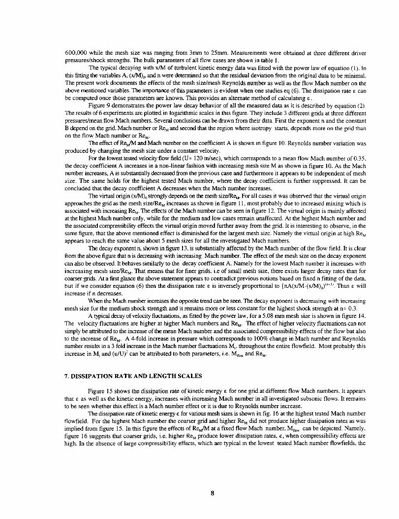
TheeffectofRer_MandMachnumberonthecoefficientA isshowninfigure10.Reynoldsnumbervariationwasproducedbychangingthemeshsizeunderaconstantvelocity.

Forthelowesttestedvelocityflowfield(U=120rn/sec),whichcorrespondstoameanflowMachnumberof0.35,thedecaycoefficientA increasesinanon-linearfashionwithincreasingmeshsizeMasshowninfigure10.AstheMachnumberincreases,Aissubstantiallydecreasedfi'omthepreviouscaseandfurthermoreit appearstobeindependentofmeshsize.ThesameholdsforthehighesttestedMachnumber,wherethedecaycoefficientisfurthersuppressed.ItcanbeconcludedthatthedecaycoefficientA decreaseswhentheMachnumberincreases.

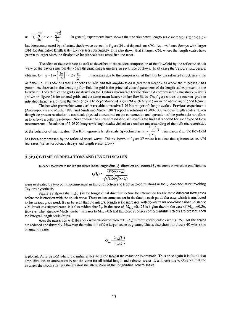
Thevirtualorion(x/M)0stronglydependsonthemeshsize/ReM.Forallcasesit wasobservedthatthevirtualoriginapproachesthegridasthemeshsize/ReMincreasesasshowninfigure11,mostprobablyduetoincreasedmixingwhichisassociatedwithincreasingR_.TheeffectsoftheMachnumbercanbeseeninfigure12.ThevirtualoriginismainlyaffectedatthehighestMachnumberonly,whileforthemediumandlowcasesremainunaffected.AtthehighestMachnumberandtheassociatedcompressibilityeffectsthevirtualoriginmovedfurtherawayfromthe_id.It isinterestingtoobserve,inthesamefi_mare,thattheabovementionedeffectisdiminishedforthelargestmeshsize.NamelythevirtualoriginathighReMappearstoreachthesamevalueabout5meshsizesforalltheinvestigatedMachnumbers.

Thedecayexponentn,showninfi_mare13,issubstantiallyaffectedbytheMachnumberoftheflowfield.It isclearfromtheabovefi_marethatnisdecreasingwithincreasingMachnumber.Theeffectofthemeshsizeonthedecayexponentcanalsobeobserved.ItbehavessimilarlytothedecaycoefficientA.NamelyforthelowestMachnumberit increaseswithincreasingmeshsize/ReM.Thatmeansthatforfinergrids,i.eofsmallmeshsize,thereexistslargerdecayratesthanforcoarsergrids.Atafirstglancetheabovestatementappearstocontradictpreviousnotionsbasedonfixednfittingofthedata,butif weconsiderequation(6)thenthedissipationrateeisinverselyproportionalto{nA(x/M-(x/M)J"+_.Thusewillincreaseif ndecreases.

WhentheMachnumberincreasestheoppositetrendcanbeseen.Thedecayexponentisdecreasingwithincreasingmeshsizeforthemediumshockstren_handit remainsmoreorlessconstantforthehighestshockstrengthatn-_0.3.

Atypicaldecayofvelocityfluctuations,asfittedbythepowerlaw,fora5.08mmmeshsizeisshowninfigure14.ThevelocityfluctuationsarehigherathigherMachnumbersandReM.TheeffectofhighervelocityfluctuationscannotsimplybeattributedtotheincreaseofthemeanMachnumberandtheassociatedcompressibilityeffectsoftheflowbutalsototheincreaseofReM. A 4-fold increase in pressure which corresponds to 100% change in Mach number and Reynolds

number results in a 3 fold increase in the Mach number fluctuations M,, throughout the entire flowfield. Most probably thisincrease in M, and (u/U) _"can be attributed to both parameters, i.e. MNo_ and Re M.

7. DISSIPATION RATE AND LENGTH SCALES

Figure 15 shows the dissipation rate of kinetic energy e for one grid at different flow Mach numbers. It appears

that E as well as the kinetic energy, increases with increasing Mach number in all investigated subsonic flows. It remainsto be seen whether this effect is a Mach number effect or it is due to Reynolds number increase.

The dissipation rate of kinetic energy • for various mesh sizes is shown in fig. 16 at the highest tested Mach numberflowfield. For the highest Mach number the coarser grid and higher Re Mdid not produce higher dissipation rates as was

implied from figure 15. In this figure the effects of ReM/M at a fixed flow Mach number, MnoW can be depicted. Namely,figure 16 suggests that coarser grids, i.e. higher ReMproduce lower dissipation rates, e, when compressibility effects arehigh. In the absence of large compressibility effects, which are typical in the lowest tested Mach number flowfields, the

reverseinfluenceofthemeshsizeone non-dimensionalized by the mean velocity and mesh size has been found as is shown

in figure 17. In this figure, non-dimensionalized e for the lowest tested flowfield of Mnow=0.35 is plotted for various meshsizes. The reverse trend is observed for eM/U 3 in the absence of strong compressibility effects. Since the mean flowfield

velocity U is equal for all plotted cases the effect presented in this figure is mainly due to the Mesh size M and ReM. In thiscase, the coarser _id with the largest mesh size and highest Re Mshows the largest non dimensionalized dissipation rate of

kinetic energy. For even higher mean Mach number flowfields (see figure 18) the effect of compressibility is rather strikingwhere, once more, the opposite trend of the dependence of eM/U 3 to the mesh size/Re Mis shown. For the medium testedMach number flowfield case the effect of the grid's mesh size becomes obvious when figure 19 is studied. From this figure

it can be summarized, that the coarser _ids with the _eater mesh sizes and highest Re Mflowfield produce a lower

dissipation rate e. The dissipation rate of kinetic energy for the medium tested Mach number foUows the trend that existslbr the highest tested Mach number and therelbre suggest that the presence of compressibility effects are felt in this flowfieldtoo. The difference and the influence of the compressibility effects for both flowfields can be estimated upon closer

investigation of fi_mares16 and 19. For almost a 4-fold increase in the mesh size and Re Mthe dissipation rate decreased 10times for M_,,w---0.6 and approximately 5 times for the Mnow=0.475 flowfield. Ttz.is verifies that higher Mach number

flowfields introduce higher compressibility effects.The dissipative length scale L_ indicates how fast the advected turbulent kinetic energy q2 at a given location, is

dissipated in to heat. As Mach number increases the results of the present investigation show that the dissipative length scaleL_ increases although the dissipation rate of turbulent kinetic energy, c, also increases. This increase in L e is attributed tothe increase in q'- with Mach number which apparently is larger than the corresponding increase of e.

A typical result is shown in figure 20 for the flow at three different Mach numbers and for the same mesh size. It

is interesting to observe that for the highest mean flow Mach number the dissipation length scale increased much more thanfor the medium case. Higher compressibility effects and higher ReM are the only logical parameters than can cause such adrastic increase. The effect of the gnd's mesh size on the dissipation length scale is shown in figure 21. The dissipation

length scale L_ increases with increasing mesh size and Re M. From this figure it can be seen that for the same mean Machnumber a 5-fold increase in L_ occurs for a 3-fold increase in the mesh size/ReM. The pivotal effect that the vid size exerts

on the length scales in the flowfield should be clear by now. It is apparent from both previous figures that the dissipation

length scale strongly depends on x/M.

,,2The effect of Mach number on the Taylor's microscale computed from E = 15v = 15v --_ is shown in

fi_tre 22 for three different Mach numbers and for the same mesh size. The Taylor's microscale appears to increase with

increasing Mach number. Increase of the Taylor's microscale is also observed for the flowfield produced by coarser grids.This is shown in figure 23 where four different grid sizes at the same Mach number are plotted. It is clear that the coarser

the grid, larger mesh size, the greater the Taylor's microscale. The dependance (increase) with increasing x/M is evident,as shown earlier for the dissipation length scale, is also shown for the Taylor's microscale.

As the Mach number increases the Kolmogorov's len_w.hscale (rl) decreases as it can be seen in figure 24 for

M=5.08 mm. This result was expected since the dissipation rate of kinetic energy increases with increasing Mach number.

Thus from the definition of _1= _ the previous result was obtained.

The effect of the different mesh sizes on the viscous scales can be shown for a constant velocity flowfield but with

different mesh size turbulence generating grids. Experimental results showed that the Kolmogorov's length scale increasesas the mesh size increases. Figure 25 presents four different mesh sizes for a decaying flowfield at a constant mean Machnumber of 0.6. Similar results are obtained for the rest of the tested flowfields.

The last two figures (24 and 25) can verify the influence of the compressibility effects on the viscous scales. Since

rl increases as the mesh size and ReM increase, then one might expect figure 25 to show an increase of 11when ReM is

increased by increasing the velocity of the flowfield only (mean flow Mach number). The latter trend is shown in figure 24to be incorrect and rather high compressibility effects associated with the corresponding flowfields are credited for suchbehavior ofrl. Namely for the case of the viscous scales, compressibility effects appear to suppress their size. The abovementioned measurements indicate values of _1 ranging from 0.015 to 0.06 mm The size of the probes expressed in terms

of Kolmogorov's length scales appears to be rl _=lw/_l=13 for the geatest scales and 52 for the smallest scales. The scalesat error start at about half of these values, 7 and 26 respectively. Based on these values, which determine the upper limit

of the valid part of the spectrum, estimates of the spectral power density of the spatially filtered scales have been obtainedfrom Wyngaard's (1968) work for subsonic flows. It appears that the spatially filtered scales amount to about 15% of the

totalspectraldensityofvelocityfluctuationstor measurements close to the _id where 11 is small and less than 4% formeasurements where rl is larger. The high resolution of the hot wire probes allows us to conclude that the results obtainedin regard to the compressibility effects on the viscous scales are not biased.

8. THE INTERACTION OF DECAYING TURBULENCE

Figure 26a shows the decay of the Mach number fluctuations downstream of the 2x2 (2 meshes per inch) gridbefore the interaction. It can be seen that the experimental data obey very closely the power law decay described by equation

2. It also clear that M, increases with the mean flow Mach number M i.e. driver pressure as shown earlier. After the passageof the shock the flow field changes. Velocity fluctuations in the longitudinal direction increase and Mach number fluctuations

(shown in fi_mare26b) are changed also but not very drastically because the amplification of velocity fluctuations u is offset

by an increase in mean temperature due to the compression. Thus M, after the interaction sometimes is higher and sometimesis lower than before the interaction.

Figure 27a demonstrates the power law decay behavior of all the measured data as it is described by equation (2).

The results of 6 experiments are plotted in logarithmic scales in this figure. They include 3 different grids at three differentpressures/mean flow Mach numbers and they correspond to the data shown in fig. 9.

The results after the passage of the shock are shown in figure 27b. The large region of a linear behavior in this log-log plot indicates that the flow follows the same power law decay with different n, B and (x/M)0. This is an indication thatthere is a quick return to isotropy of the flow after the passage of the shock which can be considered as a strong axisymmetricdisturbance imposed on the isotropic field.

Determination of the virtual origin (x/M)o, decay exponent n and decay coefficient B was accomplished by fittingthe experimental data to the power law of equation (2) so that the standard mean square deviation is minimized (seeMohamed and LaRue, 1990). Figure 28 shows a typical variation of the decay exponent n before and after the interaction

with the shock wave of M_-_1.37 for various mesh sizes of grids. The results show that n is a function of the mesh size i.e.initial conditions before the interaction and that these values are substantially less than one. The effect of the shock

interaction is very dramatic and depends on the M_, Mn,wand initial conditions.Figure 29 presents the ratio of the decay coefficient, after the interaction with the shock to that before the

interaction, nJno. It can be seen that this ratio is always _eater than one for all investigated cases. In the lowest subsonic

flow interaction with a M,-_ 1.2 shock, this ratio appears independent of initial conditions. This is in agreement withMohamed and LaRue, 1990. In the case of M_,w---0.475this ratio is very high at small ReM and decreases to 1.25 at high ReM

where it remains independent of it. At higher Mach numbers this ratio increases dramatically with ReM. Thus nJn Udependson initial conditions, flow Mach number Mnowand shock stren_h M,.

It was shown previously in section 6 that the velocity fluctuations are higher for higher mean Mach numberflowfields. The opposite trend is evident after interaction in figure 30 where the flow-field is compressed by the reflected

shock wave. Namely, after the interaction of the flow with the reflected shock wave, the lower Mach number flow possessesthe higher velocity fluctuations. Similar results are observed for the other coarser grids (larger mesh sizes). The effect of

the grid size on velocity fluctuations can be verified from figures 30 and 3 I. It appears that there exists higher velocityfluctuations in flowfields produced by finer grids with lower Re M.

From the information on the decay of velocity fluctuations and the use of the power law, the dissipation of kineticenergy for the compressed by the shock wave flowfield can be obtained by:

'-'-''I2 [M uj0] t-- j

where the subscripts u and d refer to the mean flow upstream and downstream of the shock wave respectively. In generalit can be concluded that the dissipation rate of kinetic energy (e) is drastically decreased after the interaction of the flowfield

with the reflected shock wave. Typical results of e are shown in Figures 32 and 33 for two different grids at the highestMach number tested.

From the analysis of the dissipation rate of kinetic energy the dissipative length scale, L¢, can be calculated

10

3

as -U aq--i = e = _ . In general, experiments have shown that the dissipative len_h scale increases after the flow3x Lc

has been compressed by reflected shock wave as seen in figure 34 and depends on x/M. As turbulence decays with larger

x/M, the dissipative len_th scale (L0 increases substantially. It is also shown that at larger x/M, where the length scales havegown to larger sizes the dissipative length scale was amplified the most.

The effect of the mesh size as well as the effect of the sudden compression of the flowfield by the reflected shockwave on the Taylor's microscale (k) are the principal parameters in such type of flows. In all cases the Taylor's microscale,

obtained by e = 15v = 15v L 2 , increases due to the compression of the flow by the reflected shock as shown

in figure 35. It is obvious that _, depends on x/M and this amplification is greater at larger x/M where the microscale has_own. As observed in the decaying flowfield the grid is the principal control parameter of the length scales present in the

flowfield. The effect of the gTid's mesh size on the Tayior's microscale for the flowfield compressed by the shock wave isshown in figure 36 for several grids and the same mean Mach number flowfields. The figure shows the coarser _ids tointroduce larger scales than the finer _ids. The dependance of _. on x/M is clearly shown in the above mentioned figure.

The hot wire probes that were used were able to resolve 7-26 Kolmogorov's length scales. Previous experiments(Andreopoulos and Muck, 1987, and Smits and Muck, 1987) report resolutions of 300-1000 viscous length scales. Even

though the present resolution is not ideal, physical constraints on the construction and operation of the probes do not allowus to achieve a better resolution. Nevertheless the current resolution achieved is the highest reported for such type of flow

measurements. Resolution of 7-26 Kolmogorov's length scales yielded an excellent understanding of the bulk characteristics

of the behavior of such scales. The Kolmogorov's len_h scale (11) defined as _ --- i , increases after the flowfield

has been compressed by the reflected shock wave. This is shown in figure 37 where it is clear that "q increases as x/Mincreases (i.e. as turbulence decays and length scales grow).

9. SPACE-TIME CORRELATIONS AND LENGTH SCALES

In order to estimate the length scales in the Ion_tudinal _ _direction and normal _: the cross correlation coefficients

r_j(_0 - ui(x)uj(x+_)

were evaluated by two point measurement in the _, direction and from auto-correlations in the __direction after invoking

Taylor's hypothesis.Figure 38 shows the Lt _(_ _) in the longitudinal direction before the interaction for the three different flow cases

before the interaction with the shock wave. There exists some scatter in the data in each particular case which is attributed

to the various grids used. It can be seen that the integal length scale increases with downstream non-dimensional distancex/M for all investigated cases. It is also evident that L_ in the case of Mnow=0.475 is higher than in the case of Mn,,,_=0.36.

However when the flow Mach number increases to Mno,.--0.6 and therefore stronger compressibility effects are present, then

the integral length scale drops.After the interaction with the shock wave the distribution ofL_ t(_ _)is more complicated (see fig. 39). All the scales

are reduced considerably. However the reduction of the larger scales is greater. This is also shown in figure 40 where theattenuation ratio

is plotted. At large x/M where the initial scales were the largest the reduction is dramatic. Thus once again it is found that

amplification or attenuation is not the same for all initial length and velocity scales. It is interesting to observe that thestronger the shock strength the _eatest the attenuation of the longitudinal length scales.

11

Thetwopointcorrelationr_(_2)inthelateraldirection_2ofthelongitudinalvelocityfluctuationsisshowninfigure41.Thesedatawereobtainedbyaspeciallydesignedcrosscorrelationprobeofsixparallelwiresandthreetemperaturewiresseparatedfromeachotherbylmm.Notallthecurvescrossthezerolineandthereforeit isverydifficulttointe_atetheminordertoobtaintheclassicallydefinedlengthscaleinthelateraldirection.Howevertheslopesofthesecurvesareindicativeoftheirtrend.ItisratherobviousthatthelengthscalesbeforeinteractionarereducedwithincreasingflowMachnumber.Thisbehaviorisverysimilartotha_,ofL__(__).Aftertheinteraction,howevertheleng_dascaleL__(_2)increasesinthefirsttwocasesanddecreasesinthestrongestinteraction.

InordertoinvestigatetheeffectofinitialconditionsonthiscorrelationatthehighestflowandshockMachnumberwherethelateralscalesareshowntoreduce(fig.41)variousgridswereused.Thedatashowninfigure42indicatethatthecorrelationincreasessubstantiallyinthecaseofthefinestgid, 8x8withthelowestRex,aftertheinteraction.Howeverthecoarsergrid,2x2gridwiththehighestRex=737,showsthegreatestattenuationinthelateralintegralscaleofturbulenceaftertheinteraction.

Theeffectoftheshockstrengthonthevelocityfluctuationsisshowninfig.43.Forthelxl grid,it appearsthattheamplificationofturbulencefluctuationsdefinedas

increaseswithdownstreamdistanceforagivenflowcaseandinteraction.AstheMnowincreasesGualsoincreases.Forfinergridstheeffectsofshockinteractionarefeltdifferently.Forthe2x2_idforinstance,thedatashowthatinthefirstcaseofapracticallyincompressibleupstreamflowinteractingwitharatherweakshock,amplificationofturbulenceoccursatx/M>35.Theamplificationisgreaterwhen_ increasesto0.436.However,whencompressibilityeffectsintheupstreamflowstarttobecomeimportantnoamplificationtakesplace(Guisabout1).

Somemoredramaticeffectsofcompressibilityareillustratedinfigure44,wheretheamplificationGuisplottedforthecaseofafinergridwithmeshsize5x5.TheinteractionofaweakshockwithapracticallyincompressibleturbulentflowproducesthehighestamplificationofvelocityfluctuationswithGureachingavaluecloseto2.AstheM_,_wincreases,GudecreasesandatMnow=0.576aslightattenuationoccursatdownstreamdistances.It isthereforeplausibletoconcludethatforhighshockstrength(highMachnumber)compressibilityeffectscontrolthevelocityfluctuationswhicharegeneratedbyfinegridsandnoamplificationofturbulentkineticenergyisobserved.

HannapelandFriedrich(1995)havealsoshownintheirDNSworkthatcompressibilityeffectsintheupstreamreduceturbulenceamplificationsignificantly.TheLinearInteractionAnalysisofRibner,whichwasinitiallydevelopedforanincompressibleisotropicturbulentfield,predictsamplificationofturbulencefluctuations.Mahesh,LeleandMoin(1997)haveshownrecentlythatLIAaswellasDNSmayshowacompletesuppressionofamplificationofkineticenergyiftheupstreamcorrelationbetweenvelocityandtemperaturefluctuationsispositive.It isthereforepossiblethatincaseofveryfinegridsandhighMachnumberflowswherethedissipationrateofturbulentkineticenergyishigh(seefigures15and16)thatentropyfluctuationsmayberesponsibleforcompletelysuppressingturbulenceamplification.

RapidDistortionTheory(seeJacquinetal.,1993)alsoshowssubstantialdampingofamplificationduetopressurefluctuations.OurpressurefluctuationdataatthewallbeneaththeboundarylayershowsignificantlyhigheramplificationofpressurefluctuationsGp(seefigure50)forfinergrids.If thedampingeffectsofpressurewereignoredRDTleadstothefollowingsimplerelationforGu

whereC=pd/p,.InthepresentexperimentsCisbetween1.25to1.7whichindicatesthatG_isbetween1.09to1.3.Althoughthedecayexponentincreasesafmrtheinteraction(seealsoJacquin,1991),thedissipationrateofkinetic

energydecreasesbecauseeisproportionalto:

Attenuationofthedissipationrateofkineticenergyisoftheorderof0.3forallthe_idstestedatthehighestMach

12

number. A 3-fold decrease of the dissipation rate of kinetic energy is found for the interacted (compressed) flow as shown

in figure 45. It is interesting to observe that at this high mean Mach number which produced flowfields with the greatest

compressibility effects, the grid's mesh size appears to be inconsequential to the attenuation of the dissipation rate of kinetic

energy.

The effect of the shock strength / mean flow Mach number on the attenuation of the dissipation rate was found when

the mesh size was kept constant and data presented for experiments of different mean flow Mach numbers is shown in figure

46. It is clear that the higher the mean flow Mach number/compressibility effects, the =,greater the attenuation of the

dissipation rate of kinetic energy. A 3-fold attenuation of c is observed for high (Mno_=0.7) and medium (M,a,>_=0.5) shock

strengths and a 2-fold attenuation for the lowest case (Mnow--0.3). The attenuation of e after the interaction of the flowfield

with the reflected shock wave was also independently calculated by inte_ating the wavenumber spectrum before and after

the interaction. The ratio of the two inte_als is shown in the same figure (scattered points). It is clear that both methods

present the attenuation of the dissipation rate of kinetic energy after interaction with the shock wave.

The dissipative teng_th scales L_, which express the distance within which the advected turbulent kinetic energy is

directly dissipated, increase after the interaction with the shock because the dissipation rate is attenuated.

Figure 47 shows the amplification of the dissipative length scales defined as:

Le,d

G L -

Le,u

where L_._ and L_.o are the length scales downstream and upstream of the shock respectively. At each location x/M, Lo and

turbulence intensity are different. The results suggest that at large x/M where L e is indeed large and velocity fluctuations are

small, L_ is amplified more. The data also indicate that Gk is increased with shock strength.

The present high resolution measurements, with hot-wire length of the order of 8 or less viscous units, allowed for

analysis of the data of the viscous scale level. Most of the previous experiments of compressible turbulence were carried out

with resolution of 300 to 1000 viscous lenph scales. Figure 48 shows the amplification of the viscous scales defined as:

G _'qd

.q

where .q=

It is interesting to observe that G n is considerably smaller than Gt_ and that it behaves somehow differently. Gn decreases

with downstream distance and shock strength. The different behavior of G,_, GL_ and G n clearly suggest that the result of

the shock interaction is not felt uniformly across all the length scales of the flow: Larger eddies are amplified or attenuated

more than smaller eddies. Both length scales Le and 11 depend on the dissipation rate e which in all experiments has been

found to be reduced after the interaction to about 0.2 of the upstream value. The DNS of Lee et al. (1993) indicate a moderate

increase in e after the shock interaction. This difference between the present experimental results and those of DNS leads

to different, qualitatively, description of the effect of the shock interaction on leng+,.h scale. In order to further assess the

behavior of len_,mt_scale independently from e, the Taylor's microscale _'_=L(.__) 2] has been computed from the time

derivative of u velocity after invoking Taylor's hypothesis. The amplification ratio

together with the amplification of the same scale _., obtained from:

Ii"E=--

2

is plotted in figure 49

13

ThedataclearlyindicatethatTaylor'smicroscaleincreasesaftertheinteraction.Amplificationofpressurefluctuationsisnotthesameforalldistancesawayfromthe_id. Figure50showsthe

efl_tofamplificationofpressurefluctuationsforthreedifferentgrids.The10xl0gridgeneratedhigherpressurefluctuationsthantheothertwogrids(4x4,2x2)andthusamplificationwashigher.Fromthesamepictureonecanalsodepicttheamplificationofpressurefluctuationsatrelativelylargedownstreamdistances.It isinterestingtopointoutthatatlargenon-dimensionaldistances(non-dimensionalizedwiththegridsize)x/M=720thepressurefluctuationsarestillamplified.

10. CONCLUDING REMARKS

The interaction of an isotropic and homogeneous turbulent flow with a strong axisymmetric disturbance, like a

normal shock, is the best paradigm of a test case where a turbulence model of the LES or RANS class can be evaluated. The

absence of turbulence production and the simplified flow geometry can expose the model's strengths and weaknesses.

Experimental realization of a homogeneous and isotropic flow interacting with a normal shock in the laboratory

is a formidable task. There are two major difficulties associated with this: Setting up a compressible and isotropic turbulent

flow is the first one and the generation of a normal shock interacting with flow is the second. These two problems may be

interrelated and may be not independent from each other. As a result of these difficulties two different categories of

experiments have been carried out. The experimental set up in shock tubes offers the possibility of unsteady shock

interactions with isotropic turbulence of various lengrth scales and intensity.

a. Compressibility effects in the incoming flow

The effects of compressibility in a nearly homogeneous and nearly isotropic flow of decaying turbulence have been

investigated experimentally by carrying out high resolution measurements in a large scale shock tube research facility. A

variety of grids of rectang'ular mesh size was used to generate the flow field. The Reynolds number of the flow based on the

mesh size Re Mwas ran_ng from 50x103 to 400x103 while the turbulent Reynolds number Re x based on Taylor's microscale

_. was between 200 and 700 which constitutes one of the highest ever achieved in laboratory scale flow. The range of Mach

number of the flows investigated was between 0.3 and 0.6 which was low enough to assure a shock free flow and reasonably

high enough to contain compressibility effects.

The isotropy of the present flow was verified experimentally and it was found to be within the range reported for

incompressible flows. In thcL it was established for the first time that isotropic compressible turbulence at moderate subsonic

Mach numbers can be setup experimentally. The decay of Mach number fluctuations was found to follow a power law similar

to that describing the decay of incompressible isotropic turbulence

where B, (x/M) o and n are constants depending on the flow Mach number as well as on the Re u. It was possible to investigate

the effects of the Mach number and Re Mon the flow development independently from each other. The decay coefficient B

and the decay exponent n decrease with increasing Mach number while the virtual origin (x/M),, increases with increasing

Mach number.

Most probably the mechanism responsible for this effect is the inherently low _owth rate of compressible shear

layers emanating from the cylindrical rods of the grid. Figure 51a shows a typical merging of shear layers to form an

isotropic flow in the case of incompressible flows. The case of compressible shear layers is depicted in figure 5 lb where

it is shown how a lower _owth rate can result in longer virtual orion. If a shock wave had been formed in the vicinity of

the grid as in the case ofZwart et al. (1996) the decay rate would have been drastically affected. Shock waves in the present

case is more likely to appear at Mach numbers higher than 0.7 because the open area of the grids used is _eater than that

required to choke the flow through the grids. Therefore it is plausible to attribute the present results to the lower _owth rate

of compressible shear layers.

The Taylor's microscale appears also to increase with increasing Mach number. The Kolmogorov's length scale

_1 decreases as the Mach number of the flow increases. The results also indicated that 11 increases as the mesh size increases

14

Table 2, presented at the end of this section, summarizes the conclusions for the parameters that were investigated in this

work and their response to an increase of the mean flow Mach number and an increase in the mesh size/Re M. In this table

three symbols are used: ( ) ) represents that the parameter increases with increasing Mt_o_.or increasing mesh size/Re M,

( i ) represents that the parameter decreases with increasing M_owor increasing mesh size/Re_ and finally ( I ) representsthat the parameter because of compressibility effects does not present a specific trend with increasing M,a,,_or increasingmesh size/Re M.

b. The interaction with the shock

An experimental study of the interaction of a normal shock wave with decaying _id generated nearly isotropicturbulence has been performed using time resolved pressure, velocity, temperature and Mach number measurements in a

shock tube. Spatial resolution of the order of 7-26 Kolmogorov viscous length scales was achieved in the measurements ofturbulence. A variety of turbulence generating grids provide a wide range of turbulence scales with flow Mach numbersranging from 0.3 to 0.7 and shock Mach numbers from 1.2 to 1.6.

The present results verified a proposed power law decay of the turbulent Mach number M_ in the range of 0.01 to

0.1. Longitudinal velocity fluctuations were amplified through the shock.The results show that the decay exponent, n, is a function of the mesh size i.e. initial conditions before the

interaction, and that its value is substantially less than one. The effect of the shock interaction is very dramatic and produces

a dependance of n on the M_, M)a,,_and initial conditions. The decay exponent after interaction is _eater than the oneobtained before interaction for all investigated cases.

Amplification of velocity fluctuations after the interaction was found in all case involving turbulence produced bycoarse grids. This amplification increases with shock strength and flow Mach number. In the case of fine grids, amplification

was found in all interaction with low Mn,,_.while at higher Mnowreduced or no amplification of turbulence was evident.These results indicate that the outcome of the interaction depends strongly on the upstream properties of the flow.

Inte_al lengxh scales in the lon_tudinal direction were reduced after the interaction in all investigated flow cases.The same length scales in the normal direction increased at low Mach numbers and decrease during stronger interactions.

It appears that at the weakest of the present interactions the eddies are compressed in the longitudinal direction drasticallywhile their extent in the normal direction remains relatively the same. As the shock strength increases the lateral length scale

increases while the lon_tudinal decreases. At the strongest interaction of the present cases the eddies are compressed in bothdirections. However, even at the highest Mach number case the issue is more complicated since amplification of the lateral

scales has been observed in fine grids. Thus the outcome of the interaction strongly depends on the initial conditions. Thedissipation rate was reduced through the interaction while all dissipative length scales were found to increase. DNS results

of Lee et al. (1994) have indicated a small increase of dissipative length scales through weak shock interactions. For shockstrengths greater than 1.25 DNS predicts a substantial decrease in L,. The Rex of the DNS was between 12 and 22 which

is considered lower than that in the present experiments and may be the cause of this disa_eement between experiments andDNS.

The present results clearly show most of the changes, either attenuation or amplification occur at large x/M

distances where the len_da scales of the incoming flows are high and turbulence intensities low. Thus large in size eddieswith low velocity fluctuations are affected the most by the interaction with the shock.

Table 3 summarizes in a similar fashion as before the conclusions for the parameters that were investigated in this work andtheir response to an increase of the mean flow Mach number and an increase in the mesh size/ReM.

15

REFERENCES

Adamson, T.C. and Messiter, A.F., 1980, "Analysis of two Dimensional Interactions Between Shock Waves and Boundary

Layers", Ann. Rev. Fluid Mech., vol.12, 103.

Agui, J., 1998, "Vorticity transfer through shock waves," PhD Thesis, City University of New York, (in preparation ).

Alem, D., 1995, "Analyse experimentale d' une turbulence homogene en ecoulement supersonoc soumise a un choc droit",

These de doctorat, Univerite de Poitiers.

Andreopoulos, J. and Muck, K.C., 1987, "Some New Aspects of the Shock-Wave Boundary Layer Interaction in

Compression Ramp Comer", J. Fluid Mech., vol. 180, 405.

Ardonceau, P.L, 1984, 'The Structure of Turbulence in a Supersonic Shock-Wave/Boundary Layer Interaction", AIAA J.,

vol.22 (9), 1254.

Anyiwo, J.C. and Bushnell, D.M., 1982, "Turbulence Amplification in Shock-Wave Boundary Layer Interaction", AIAA

J., vol.20, 893.

Barre, S., Allem, D., and Bonnet, J. P., 1996, "Experimental study of normal shock/homogeneous turbulence interaction",

AIAA J., vol. 34(5), pp. 968-974.

Blin, E., 1993, "Etude experimentale de l'interaction entre turbulence libre et une onde de choc", These de doctorat,

Universite Paris 6.

Briassulis, G.K., 1996, "Unsteady Nonlinear Interactions of Turbulence with Shock Waves", Ph.D. Thesis, City College of

CUNY.

Batchelor, G. K_, and Townsend, A. A., 1949, "The Nature of Turbulent Motion at High Wave Numbers," Proc. Roy. Soc.

A, 199, 238.

Bennett J. C. and Corrsin S., 1978, "Small Reynolds Number Nearly Isotropic Turbulence in a Straight Duct and

Contraction," Phys. Fluids, 21 (12), 2129.

Betchov, R. and Lorenzen, C., 1974, "Phase Relations in Isotropic Turbulence," Phys. Fluids, 17 (8), 1503.

Briassulis, G., Honkan, A., Andreopoulos, J., and Watkins, B. C., 1995, "Applications of Hot-Wire Anemometry in Shock

Tube Flows," Exp. in Fluids, vol 19, 29.

Buckingham, A., C., 1990, "Interactive Shock Structure Response to Turbulence," AIAA Paper No 90-1642.

Budwig, R., Zwart, P., J., Nguyen, V., and Tavoularis, S., "Grid Generated Turbulence in Compressible Streams," ASME,

2nd Symp. on Transitional and Turbulent Compressible Flows, Aug. 1995.

Cambon, C., Coleman, G.N., and Mansour, N.N., 1993, "Rapid distortionanalysis and direct simulation of compressible

homogeneous turbulence at finite Mach number", J. Fluid Mech., vol. 257, pp. 641-665.

Chu, B.T. and

Mech.,vol.3,

Debieve, J.F.

Dosanjh, D.S.

Kovasznay, L.S.G., 1957,"Non-linear Interactions in a viscous Heat-Conducting Compressible Flow", J. Fluid

494.

and Lacharme, J.P., 1985, "A Shock Wave Free Turbulence Interactions", IUTAM Conference, Paris.

and Weeks, T.M., 1964, "Interaction of a Starting Vortex as well as Karman Vortex Streets with Traveling

16

ShockWave",AIAAPaperNo.64-425.

Favre,A.,1965,"EquationsdesGazTurbulentsCompressiblesI,"J.M6c.,vol4,361.

Frenkiel,F.,N.,andKlebanoff,P.,H.,1971,"StatisticalPropertiesofVelocityDerivativesinTurbulentField,"J.FluidMech.,vol.48,183.

Frenkiel,F.,N.,Klebanoff,P.,H.,andHuang,T.,T.,1979,"GridTurbulenceinAirandWater,"Phys.Fluids,22(9), 1606.

Gutmark, E., J., Schadow, K., C., and Yu, K., H., 1995, "Mixing Enhancement in Supersonic Free Shear Flows," Annu. Rev.

Fluid Mech., vol. 27, 375.

Haas, J.F., and Sturtevant, B., 1987, "Interaction of Weak Shock Waves with Cylindrical and Spherical Gas

Inhomogeneities". J. Fluid Mech., vol.181,41.

Hannappel, R., and Fridrich, R., 1995, "Interaction ofisotropic turbulence with a normal shock-wave", Appl. Sci. Res.. Vol.

54, pp. 205-221.

Hancock, P. E. and Bradshaw P., 1983, "The Effect of Free-Stream Turbulence on Turbulent Boundary Layers," J. Fluid

Eng.. vol. 105,284.

Hayakawa, K., Smits, A. J., and Bogdonoff, S. M., 1984, "Turbulence Measurements in a Compressible Reattaching Shear

Layer," AIAA Journal, vol. 22, 889.

Hartung, L.C. and Duffy, R.E., 1986 "Effects of Pressure on Turbulence in Shock-Induced Flows", AIAA Paper No 86-

0127.

Hesselink, L. and Sturtevant, B., 1988, "Propagation of Weak Shocks Through Random Medium", J. Fluid Mech., vol. 196,

513.

Honkan, A. and Andreopoulos, J., 1992, "Rapid Compression of Grid-Generated Turbulence by a Moving Shock Wave",

Phys. Fluids A, 4 (11).

Honkan, A. and Andreopoulos, J., 1997, "Vorticity strain-rate and dissipation characteristics in the near wall region of

turbulent boundary layers", J. Fluid Mech., vot. 350, pp. 29-96.

Honkan, A., Watkins, C.B., and Andreopoulos, J., 1993, "Experiments of Shock Wave Interactions with Free Stream

Turbulence", ASME Fluids Engineering Conference, Washington D.C.

Honkan, A. Watkins C. B. and Andreopoulos, J., 1994, "Experimental Study of Interactions of Shock Wave with Free

Stream Turbulence", J. Fluids Eng., vol. 116, 763.

Hunt, J.R.C., 1973, "A Theory of Turbulent Flow Round Two-Dimensional Bluff Bodies", J. Fluid Mech., vol.61,625.

Jacquin, Blin and Geffroy, 1993, "En Experimental Study on Free Turbulence/Shock Wave Interaction", VIII Turbulent

Shear Flows (eds: Durst et al), pp 229-248, Springer Verlag.

Keller, J. and Merzkirch, W., 1990, "Interaction of a Normal Shock with a Compressible Turbulent Flow", Exp. Fluids 8,

241.

Kistler, A., L., and Vrebalovich, T., 1966, "Grid Turbulence at large Reynolds numbers," J. Fluid Mech., vol. 26, 37.

Kuo, A. Y., and Corrsin, S., 1971, "Experiments on Internal Intermittency and Fine Structure Distribution Functions in Fully

17

TurbulentFlows,"J.FluidMech.,vol.50,285.

Lee, L. and Lele, S.K. and Moin, P., 1991, "Direct Numerical Simulation and Analysis of Shock Turbulence Interaction",

AIAA Paper No 91-0523.

Lee, L., Lele, S. K and Moin, P., 1993, "Direct Numerical Simulation of Isotropic Turbulence Interacting with a Weak

Shock Wave", J. Fluid Mech., vol. 251,533.

Lee, L., Lele, S. K. and Moin, P., 1994, "Interaction of Isotropic Turbulence with a Strong Shock Wave," AIAA Paper No94-0311.

Mahesh, K., Lele, S.K.,and Moin, P., 1997, "The influence of entropy fluctuationson the interaction of turbulence with a

shock wave", J. Fluid Mech., vol. 334, pp353-379.

Mc Kenzie, J. F. and Westphal, K. O., 1968, "Interaction of Linear Waves with Oblique Shock Waves", Phys. of Fluids, vol.

11, No 11, 2350

Mills, R. R., Kistler, A., L., O'Brien, V., and Corrsin, S., 1958, "Turbulence and Temperature Fluctuations Behind a Heated

Grid," N.A.C.A. Tech. Note No. 4288.

Mohamed, S. M., and LaRue, C. J., 1990, 'The Decay Power Law in Grid Generated Turbulence," J. Fluid Mech., vol. 219,

195.

Morkovin M.V., 1960, "Note on Assessment of Flow Disturbances at a Blunt Body Traveling at Supersonic Speeds Owing

to Flow Disturbances in Free Stream" J. Applied Mechanics, vol. 27, 223.

Ribner, H.S., 1955, "Convection of a Pattern of Vorticity Through a Shock Wave," NACA Rept. 1233.

Ribner, H. S., 1986, "Spectra of Noise and Amplified Turbulence Emanating from Shock-Turbulence Interaction," AIAA

Journal, vol. 25, 436.

Rotman, D., 1991, "Shock Wave Effects on a Turbulent Flow," Phys. Fluids A, 3 (7).

Samimy M., and Addy A.L., 1985, "A Study of Compressible Turbulent Reattaching Free Shear Layers" AIAA Paper 85-1646.

Samimy, M., Petrie, H. L., and Addy, A. L., 1986, "A Study of Compressible Turbulent Reattaching Free Shear Layers,"

AIAA Journal, vol. 24, 261.

Sekundov, A.N., 1974, "Supersonic Flow Turbulence and Interaction With a Shock Wave," Izv. Akad. Nauk SSR Mekh.

Zhidk. Gaza, March - April.

Settles, G.S., Fitzpatrick, TJ. and Bogdonoff, S.M., 1979, "Detailed Study of Attached and Separated Compression Comer

Flow Fields in High Reynolds Numbers Supersonic Flow," AIAA J., vol. 17(5), 579.

Settles, G.S., Williams, D.R., Baca, B.K. and Bogdonoff, S.M., 1982, "Reattachment of a Compressible Turbulent Free

Shear Layer," AIAA J., vol. 20, 60.

Smits S.J., and Muck K.C., 1987,"Experimental study of three shock wave/boundary layer interactions," J. Fluid

Mech.,vol.182, pp 291-314.

Spina, E., F., Smits, A., J., and Robinson, S., K., 1994, '"The Physics of Supersonic Turbulent Boundary Layers," Annu. Rev.Fluid Mech., vol. 26, 287.

18

Stewart, R. W., and Townsend, A. A., 1951, "Similarity and Self Preservation in Isotropic Turbulence," Proc. Roy. Soc.

A, 243. 359.

Tan-Atichat, J., Nagib, H., M., and Loehrke, R., I., 1982, "Interaction of Free-Stream Turbulence with Screens and Grids:A Balance between Turbulence Scales," J. Fluid Mech., vol. 114, 501.

Tavoularis S., Bennett J. C. and Corrsin S., 1978, "Velocity derivative skewness in small Reynolds number, nearly isotropic

turbulence," J. Fluid Mech., vol. 88, 63.

Tennekes, H. and Lumley, J. L., 1972. "A First Course in Turbulence", Boston, MA., MIT press.

Trolier J.W. and Duffy, R.E., 1985, "Turbulent Measurements in Shock-Induced Flows," AIAA J., vol. 23(8), 1172.

Tsinober, A., Kit, E., and Dracos, T., 1992, "Experimental Investigation of the Field of Veloci_ Gradients in TurbulentFlows," J. Fluid Mech., vol. 242, 169.

Zang T.A., Hussaini, and Bushnell, D.M., 1982, "Numerical Computations of Turbulence Amplification in Shock WaveInteractions," AIAA Paper 82-0293.

Zwart, P., Budwig, R., and Tavoularis, S., 1996, "Grid Turbulence in Compressible Flow," private communication.

19

Grid Mesh size Incident Reflec_d Flow

(Meshes/in) M (mm x mm) Shock Shock Mach # Re M

M s M r Mlnw

8x8 3.18x3.18 1.27 1.18 0.371 37138

8x8 3.18x3.18 1.342 1.25 0.461 53506

8x8 3.18x3.18 1.486 1.392 0.592 63458

5x5 5.1x5.1 1.27 1.18 0.371 59654

5x5 5.1x5.1 1.367 1.26 0.477 86315

5x5 5.1x5.1 1.469 1.388 0.576 102421

4x4 6.35x6.35 1.254 1.175 0.354 68208

4x4 6.35x6.35 1.337 1.242 0.446 105389

4x4 6.35x6.35 1.489 1.393 0.594 132921

3x3 8.5x8.5 1.227 1.166 0.321 81687

3x3 8.5x8.5 1.364 1.258 0.474 124203

3x3 8.5x8.5 1.456 1.372 0.564 215043

2x2 12.7x12.7 1.248 1.17 0.346 137319

2x2 12.7x12.7 1.328 1.231 0.436 169025

2x2 12.7x12.7 1.486 1.392 0.592 261667

1.33xl.33 19.05x19.05 1.267 1.179 0.368 200371

1.33xl.33 19.05x19.05 1.394 1.278 0.504 295721

1.33xl.33 19.05x19.05 1.504 1.405 0.607 398661

lxl 25.4x25.4 1.274 1.184 0.376 256903

lxl 25.4x25.4 1.42 1.291 0.529 438727

Ixi 25.4x25.4 1.622 1.475 0.708 577040

Re_

162

195

246

222

250

325

223

277

355

224

316

654

267

405

737

270

550

68O

296

582

735

Table 1: Bulk flow parameters of the experiments performed.

20

INCREASING INCREASING

Mno,, Re M/M

A g

(x/M) o _

n _ ._

u _ ._

M, lr t

eM/U 3 11" t

L, 17 1?

L,,(_,) _

Table 2: Summary of conclusions for the decaying isotropic flowfield.

21

INCREASING

Mflow

A

(x/M) 0 It

n t

u

M!

_M/U 3

L_ _r

INCREASING

ReM/M

SHOCK WAVE

INTERACTION

Table 3: Summary of conclusions for the interaction of a decaying isotropic flowfield with a planar shockwave.

22

//

//

/F

/

/r

/

¢w'cW-

Before interaction

MR.$

After interaction

Figure 1a: Shock wave interaction with grid turbulence.

M

x/M

Figure 1b: Grid generated flow schematic.

23

I

_3v

30000

20000

10000

0

-10000

Shock wove position

-20000 I , I , i ,0.002 0.003 0.004 0.005

3OO

200

IO0 _

0.006 0.007 0.008

Time (s)

Figure lc: Velocity and vorticity signals through the interaction with shock

Oilphrlll

o"-" It_t,; .......... ,.. ,,.,....... ,.,,,, "'"'"" "d

]'<_'._J_ '='z-_<_(=o .r_) _=o,r,:, (s :r_:, o. .

D • lip Tlsk

7.25 el m elpl©it7

(256 el |t elplelty)

Figure 2: The new shock tube facility (not to scale)

24

SIDE VIEW

..... -----O -----O -"O ......

STURBULENCEGENERATIONGRID

_m_mmmmm_mL_mdlm'/i//i//i/ll/i.,'///_.

SHOCK TUBE WALLi

Ii

FRONT VIEW (SENSORS ONLY )

Figure 3: X-Wire probe location and arrangement in the shock tube.

25

GRID

SHOCK TUBE WALL

CABLES

RAKE ASSEMBLY

FLOW

SHOCK TUBE WALL

SIDE VIEW5 PROBES

Figure 4: Side view of the rake assembly in the shock tube.(not to scale)

26

Flow Direction

Shock Wave

Shock Wave 7

Figure 5: Shock wave visualization

27

Anisotropy Tensor

0.4

0.3

0.2

0.1

0.0

-0.1

-O.2

-0.3

-0.4

0

g _ Tslnober et at, (1 992)• i_ Ts_nober et ol. 41992)• b_ Tsinober et ol. (1992)

b,1 present dora.... /_ -- t>z2presenl data----E3-.- b_ presen_ doto

• • • .1_.

I EL .. ._-

IO• A'I m "'_ / "_" _••

dh

I I I I I I _ I _ I I I

20 40 60 80 1 O0 1 20

x/M

i I ,

140

Fig_m 6: Ani_tmpy T_r bovs _VI

M=5.08 mm

1.0

0.8

0.6

0.4

0.2

0.0

-0.2

-O.4

-0.6

-0.8

•I-l-i- M_,=0.371.... &... M_,=0.477_I_ M_,=0.576

--1 .0 i I I I I I I I , • I i i i I i I , I ; 1

0 20 40 60 80 1 O0 1 20 1 40 1 60 180 200

x/M

Figure 7: Sk_s ofvel_ity fluctuations for _ diff_mt flowfiel_.

28

1,0

0.9

0.8

0.7

0.6

0.5

0.5

0.4

0.3

0.2

0.1

L_Z_

0

1:2

A

o

4-

_o

0 •

0

Bate helor & Townsend(1 949)Stewart & Townsend(1 951 )

Mills et al (1958)

Frenkle/& Klebanoff('; 97; )

Kuo &: Corsin (1 971 )Betchov & Lorenzen(1 974)

Bennett & Corsin(1 978)

"fovoulods et o1.(1978)

Mohomed & LaRue(1 990)

Honkan et al. (1 994)Present Data

-+ ur_

©

V

17

_2, , ,I,l,i I I 1 I I I I , , , I . ,,1 I I 1 I I I I . , . i . .*1 J I 1 I I I J ,, . I . i.I _ [ I I t I

2 3 4 10 2 3 4 I 00 2 5 1 000 2 5 10000

Figure 8: Skewness of the derivative of velocity fluctuations for different flowfields.

10-2

M,,..=0.321, 3x3 Grid

......... M,,0.=0.474, 5x3 Grid

........ M,,o.=0.564, 3x3 Grid

+ M_,o.=0.346.2x2 Grid

\ + M_.,=0.368.1 .33xl .33 Grid

\ :-','_ ""." M'_'_ O0:65004:11 :i_: 11:531 OO;idd

.... . - .... 'm,-.'- -_.-,.,....................

2 3 4 5 6 7 8

x/M

Figure 9: Maeh number fluctuations for various experiments

29

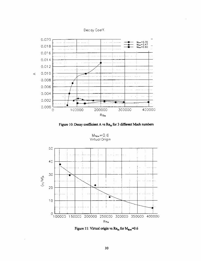
Dec oy Coeff.

<

0.020

0.01 8

0.01 6

0.01 4

0.01 2

0.01 0

0.008

0.006

0.004

0.002

0.000

D

........................ , ...................... _ .................. + Mrs,=0.30

"_ M_,=0.47:

: + Mf_.=0.60

i ih, i i i

0 100000 200000 300000 400000

ReM

Figure 10: Decay coofficient A vs Reu for 3 different Math numbers

x

5O

4O

5O

2O

10

M fJo,,= O. 6Virtual Origin

': •i i

100000 150000 200000 250000 300000 350000

' i : : i :: : ! i

D i i i i :

400000

ReM

Figure 11: Virtual origin vs Re_ for Mao,,=0.6

3O

:x:

C'-

5O

4O

50

2O

10

0

1.0

0.9

0.8

0.7

0.6

0.5

0.4

0.5

0.2

0.1

0.0

Virtual Origin

: + M_.=0.30

: _ M.f_.= 0.47

....... ! .................. :.................... : ....... ___ ...-_vi'a,k,.=n._o

• i :

: m.,< :

: \ ): .,,m :

i ? i !n !....: :

0 1 00000 200000 ,.300000 400000

Re_

Figure 12: Virtual origin vs Re_ for 3 different Math numbers

Decay Exponent

.................................................................... + Mf_.=0.30

Mf)_,,,= 0.47

: + M_,,= 0.60

: : ..P) .

............ ....................................................... I .....................

100000 200000 600000 400000

Re_

Figure 13: Decay oxponcnt n vs Re.M for 3 different Math numbers

31

M=5.08 mrr

r_

7

"6

5

'- M,I,,.,,= O. 57 ]

• ".... M,_,,= 0.477

"'.... " ........ M,_,=0.576

h _

10-4 , , , , , , , i , ,,,, ,,i.,,,., ,4 5 ,5 7 8 9 102

r , I

2

x/M

Figure 14: Decay of velocity fluctuations for various Mach numbers

Mesh size M=5.0Po mm

2"U

tO,

¢M

E

,G

40000

30000

20000

10000

0

M,o.=0.371 }M,,°.=0.477 from decay rate........ M_bo.=0.576

0 M...=0.371 }• Mn0.=0.477 fl'Olll spectra'_ M_k,.=0.576

Vk _..

\_ "'....,& "_.v .... _.......

1, r i _ ..... 1,, _ 1 ,

40 60 80 1O0

A

C "'_ --0 ....

I , 1 , I r I _ 1,

120 1 40 160 180 20',i

x/M

Figure 15: Dissipation rate of kinetic energy vs x/M for 3 different Mach numbers

32

M_lo.=0.6

_3

E

1 0 5

10 4.

103

-k \ , _. __ M=5.08mm

M=6.35 mm

\ ....... M=8.47 mm

\ -- ---- M=127 mm

...... M=19.1 mr'r"

×/M

Figure 16: Dissipation rate of kinetic energy for various mesh sizes.

M.o_=0.55

%

2

10-4

2

1 0-5

210_

' M=5.08 mm

, M=6.55 mm

• - . M=8.47 mm

' ....... M=I 2.7 mr,"

2 3 4 5 6 7 8 1 0 2 2

×/M

Figure 17: Non dimensional e for M_o_=0.35 and various mesh sizes.

33

Mr,o,,=0.6

%

10-6

54

1 01

• M=5.08 mm

",,,, _ M=6.35 mm

..... M=8.47 mm

"' \ ....... M=I 2.7 mm

\ _ M=!9,1 mrr-

\ \

---._..

%..-... ..

I , i , I , i i I , i , I ,i ,I ' j,' ' _ I , l b I

2 3 4 5 6 7 8 1 02 2

x/M

Figure 18: Non dimensional _ for lVI_---0.6 and various mesh sizes.

Mf_o,,=0.a75

2

1 05

,,.> 2

m 041

_g 2

10 3

2

102

1 0 _

_ M=508 mm

', M=6.35 mm

', ....... M=12.7 mm

_' t',/=191 tort

2 3 4. 5 6 7 8 10 2 2

x/M

Figure 19: Dissipation rate of kinetic energy for various mesh sizes at Maow=0.475

34

M=I 2.7 mm

E

3

0.6

0.5

0.4

0.5

0.2

0.1

0.0

M,_.=0.346

M,_.= 0.456 ..."

......... M,_=0.592 . .. -'"

T I , I h I , t , I , I , I , I t I k I

20 40 60 80 100 120 140 160 180 200

×/M

Figure 20: Dissipative length scale for three mean flow Math numbers.

Mf,o,.,=O. 475

0.20

0.18

0.16

0.14

0.12

E--.-- 0.10

0.08

0.06

O.04

0.02

0.00

M=5.08 mm //"/"

/M= 6.55 mm /"

j/....... M=I 27 mm /

/M=191 mrr /

j-

/

/

, I i I , I , I , I i I , F , I , i _ I

20 40 60 80 100 120 140 160 180 200

×/M

Figure 21" Dissipative length scale for several mesh sizes.

35

O.004 _ M_ 12, 7 ham

2 0.002/ .................................

ooo,/:::__.... ___0 0000_

X/M 160 180 200Fig_e 22: Tay/Or_ Z_'Crosca/e.,

O.003? "°',_ O.475 _ta_Set_,

0-0025 [ _ "°_.o._

0"0010/ ..'"'"

o.ooo_/// ....L........- ................

_u 200Fig_"e23: Taylor,s _2/Crosca_

t°r_v_at mesbsize.

36

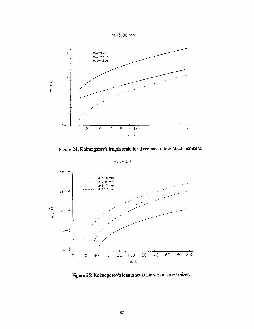
N=5.08 mm

E

M,_=0.477

......... IMt_,.= 0.575 _

4 5 6 7 8 9 _ 02 2

x/M

Figure 24: Kolmogorov's length scale for three mean flow Mach numbers.

/-'-.

£x._../

g--

5E-5

4E-5

3E-5

2E-5

1E-5

0

M,o,.,= 0.6

M=5.08 mm

M=6.35 mm

.... M=8.47mm . .............. .... "-'_........ M=I 2.7 mm

/..-):/. //

, L , I , 1 , ) i I i I i.. I i I , i , I

20 40 60 80 100 120 140 160 180 200

×/M

Figure 25: Kolmogorov's length scale for various mesh sizes.

37

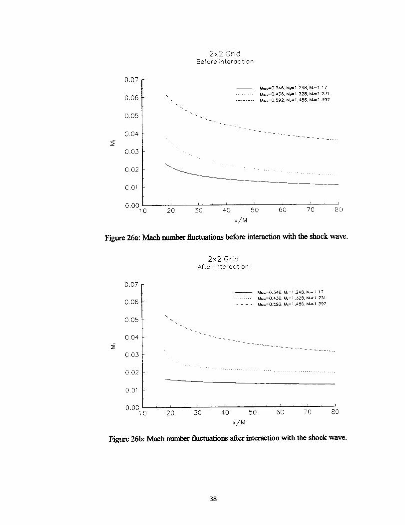
2x2 GridBefore interaction

0.07

0.06

0.05

0.04

0.03

0.02

O.01

0.0010

\

\

M.,_.,=0,346, M,_-1.248, M.=1.1 7

M,_,.,=0.436. M.=1.328. M.=t ,2.31

Mrs..= 0.592, M.=I .486. M,=1.592

I r I i I i I , I J I , I

20 50 40 50 60 70 80

x/M

Figure 26a: Mach n_ fluctuations before interaction with the shock wave.

2x2 Grid

Afterinteroction

0.07

0.06

0.05

0.04

0.05

0.02

0.01

0.00

\

M,,,_.=0.546, M.=I .248, M.=I 1 7

M,,.,.=0,436, M.=I .528. M,=1 231

M._.=0,592, M.=I .486, M,= I .592

,,, i a i I , I , I h l l I , I

0 20 30 40 50 60 70 80

x/M

Figure 26b: Mach number fluctuations after interaction with the shock wave.

38

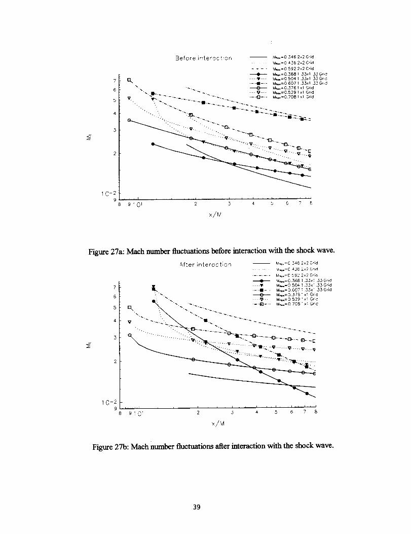
10-29

3efore interoc tion M._.-0.3462x2 Grid........ M,_=O 436 222 Grid

...... M._,=0.592 2*2 Grid

+ M_.,=0.368 1 33xl .33 Grid

I_ .... V"" MI_=O 504 1.33×1 33 Grid• ----m-.- _=0.607 1 33xl .33 Grid

"_. "_ .+ M_=0.376 1 xl Grid

""- I..._. "_'_ -. .... V"" M_,,=0.529 1 xl Grid

__ _ .... -._ . '-'-.. --.._-.- M,,o_.=O 708 1 xl Grid

•..... .:... .-...._... --m...... _.:Z:.i:z::n. - _

'::i ...... " :'-o..' .... "........ .:.-v. "--e-...

,, ,J,,,I , i , I , i , t , i , f , i , i , , , - , , ,-J

8 9101 2 5 4 5 6 7

x/M

Figure 27a: Math number fluctuations before interaction with the shock wave.

_,fter interoctiorq

I.

........ ...............' :::_ - e"_-:. :. ''e- ..... -e- .... B- - e- _r

•....... '....v .........._-W.ln.._..v ......v .....v ....

.... •",W:: _ .-_ ..........

""'i:...

M_,_.=0 346 2_2 Or;d

......... M,_.=G 436 2x2 Gr_d

........ M_,,.=0 592 2x2 GrOG

•_ M.,,.= 0.368 1.53xi .33 Grid

.... lit- -. M_,.=0.504 1.33xl .33 Grid

-"i- " M,_.=0.607 1.33xl ..35 Grid

+ M,_.=0.376 1 xl Grid

.... V"" M,_.=O 529 1 xl Grid

• -'_E]-" M_.=O 708 lxl Grid

t0-29 ,.i.,.[ i i , t , i , I , i , I , i , I . '' ,,i

8 9101 2 5 4 5 6 7 8

×/M

Figure 27b: Math number tluctuatiom after interaction with the shock wave.

39

1.0

M,,o,=0.475, M,=I .37, M,=I .25Decay Exponent

0.9

0.,6

0.7

0.6

0.5

0.4

0.3

0.2

0.1

0.00

Belore Interoction

! i .... 0... Afler InteroctTorr - .......... E..... _...........

i ,). . !................ ............. :..... ii

, 'o. , : ............... i .......... :: ....

....... ......... i............... ii_ ........

i

................ .................. i......... i .... i.i

i :

5 0 5 20 25

Mesh Size M (ram)

Figure 28: Turbulence decay exponent for various mesh sizes.

Ratio of the decoy exoonent

8

01 : t : I ....... ; ........ :..........

8 + M,_,=0.36. M,=I .26, M,=I .1 8 .... ; ....... i

7 .... &... M_,m=0.475. M,=1.37, Mr= 1.25 .... ..... '

6 _ ---'11--- Mtk,,=0.6, M,= 1.5, M,= 1.39 .... ; ........... : .......

5_:_:::::_:::::: ZIi::::::!:4:_:!:t::.!!::_!:!itt:_!:!!:!l:!:::!_!!:!::!!!i !i! !4 :i!!i!iiii i:i!i i]:::! :i:: ! i: i

_ _!!!!!! !i!!!!!!!!! . "2

;iii iiii:i:::iiii. ........._................./? .......... _...........' ........... !........ 1....... " : ....... j ........ i ..... d•.A.. : / i :

10o ! _'-'-- _ --"' ; ;

8 :::::::::::::::::::::::::::::::::::::::::::::::::::::::::::::::::: :::Ii:::::i'i::i!:i: i:i:"']::::

6 :5

1 00000 200000 50(_000 400000

ReM

Figure 29: Ratio of the decay exponem for various experiments.

4O

.,....""

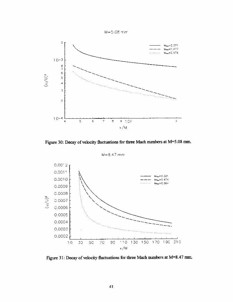
Mf_o,---0.576, M=5.08 rnrn

1 05

L) 1 04

U3

_ 3

d 2

1 03

Belore tnteroction "l

from Power= _ ......... *fter,o_eroct_ooJ"- _ • c from spectro Bef. In1.

_' "-...,,.... "'.._ • { from spec fro After ltd.

• "'.. "'"'"""'..°%°° •

'.o.

"'•,..

'°"°'...,,. •

5 6 7 8 9 102 2

x/#

Figure 32: Dissipation rate of kinetic energy l_fore and atter interaction at M=5.08mu_

Mf,o,=0.564, M=8.47 mm

1 05

1 0 4(.,)

&)

"_" 2

105

32

1 022

k Before Ioteroction _1

......... After Interoction ._ _ POWCI" law

• _, • _ from speclro Bef. Int.

'""....._ • _

'*'",,,

*-.,o.

',,,,

"-.

1 , , , I , , . I , , , I , L , t., ,I ,i,l,,,I , , I

3 4 5 6 7 8 9102 2

x/M

Figure 33: Dissipation rate of kinetic energy before and azffer interaction at M=8.47mm.

42

Mf,ow=0.321 , M=8.47 mm

Ev

0.16

0.14

0.12

0.10

O.O8

0.06

O.O4

0.02

0 00

Before lnterocgon .,-'""

......... After Interoc [ior "'"

°.,"

,"°

°

°

.°

°

°

I I i I , I I I i I _ I , I _ I , i , I

0 30 50 70 90 110 150 150 170 190 2_10

×/M

Figure 34: Dissipative length scale before and after interaction at M=8.47 mm

MfJo_=0.371 , M=5.08 mm

Ev

0.0030

0.0025

0.0020

0.001 5

0.00t 0

0.0005

..,°"

. ,,"

-- Before [n_eroction ."""

......... After Interoctlor .,-'""

°

/

0.0000 I , k , I , _ , I , f , I , i , I40 60 80 100 120 140 160 180 200

x/M

Figure 35: Taylor's microscale before and after interaction at M=5.08 mm_

43

0.006/ _"°'_o.47s

O.0o5/. _I ""_._ "_&Osm m

t ....... 'W_.6.35 mm0 "_ I "" .... _&4_

• ',JL)4/" .... M_122mm

O.oo_/ . .........0.002/_ , _..... ""'_"" . ...............

ooo,/.-:::::.:........................f ,..fi,-""..----7--- ,

o.oooL_.::.:. ..-,.._-o _o _o-__ '

6E_5 _ _"o,--o.327 ,, '5for se_,al _s h

''Vl_8.42mm _ $]IZeS.

5£_ 5 /I.. ......... ABfefOt,e Infer ..

_-, 4E = / 'e"n'"°_2'°

2E-5//

1C-5 _ ,

/0 _,90

-'" _°la2o_zo.,._ x/M , ou 75o _.__'gorovs lea_h ,., 770 790 .

scale before _ at}e_. _te_,,._. 210

""_on at M_g.47 _z_.

44

.,L.R

._J

5

4

5

.... A,...

M_,,=0.36, M,=I .26, M,=I .18

M_,,,,,=0.475, M,:I .37. M,:=I 25 •

M,_..,,=0.6, M,=I .5, M,=I .39

..... • .......... "'li'&

• i.& ........

ii-''i''' Jtl

0

0 i I i I i I i I i t , t L I t I , I , I

0 10 20 50 40 50 60 70 80 90 100

x/_

Figure 38: Longitudinal integral length scale for various experiments before interactionwith the shock wave.

-q

,X_.J

25

2.0

1.5

1.0

0.5

0.00

o

.... _o,.

"o°

°.

I;13D""_' t00

M,,o,=0.36. M,= 1 26, M,= _. 18

M,o,=0.475. M,=I .37, M,=I .25

M,oo=0.6, M,=I .5. M,=I .59

i I i i , I i I i I i I r I , I , I , I

1 0 20 50 4-0 50 60 70 80 90 1 O0

×/M

Figure 39: Longitudinal integral length scale for various experiments after interaction withthe shock wave.

45

1.0

0.9

0,8

0.7

0.6

.5 0.5o

0.4

0.5

0.2

0.1

0.00

Q """0"-- M o.=0 36. M.=I ,26, M,=I .1 8

• .... &.,. M,,o.=0.475, M,=1.57, M,=1.25

• -'g-.- Mt._.,=0.6. M.=I .5. M_=I .39

•.. Oil

'1

, I i I , I , I , I L I _ t , I , I _ I

10 20 30 40 50 60 70 80 90 100

x/M

Figure 40: Ratio of the longitudinal integral length scales for various experiments.

×/M=455x50rid

1.0

0.9

0.8

0.7

0.6

*_ 0.5E'- 0.4

0.3

0.2

0.1

0.0

-0.1

+ M.,,,.=0.371 ,M.= 'f 27. M,= 1.18 bef

Mt_,..=0.477, M.=1.367, M,=I .26 be'i

_,k_._. -'g- - M,,_,,,,=0.57,6. M+=1.46g. M,=1.3,88 bef":\_ 0 M+_,--.0.371, M,=1.27, M,=1.1 8 oft

%_'_ , - ',_-. I,,,h,,_=0+477, M,=1.367. M,=1.26 oft

_.,_X___ . - E)" .... M.o..=0.576. M,=1,469, M,=1.388 alL

,,\Xt'k

\\ " , -,,,_...........o........o

12_

0.0 0.1 0.2 0.3 0.4 0.5 0.6 0.7 0.8 0.9 1.0

_2/M

Figure 41" Space correlation in the lateral direction for three different flow cases.

46

1.0

0.9

0.8

0.7

0.6

0.5

0.4

0.5

0.2

0.1

0.0

-0.1

M_,ow=0.6, Ms=! .5, Mr=l ...39

+ x/M=36.2x2 Grid bef

+ x/kt=45, 5x5 Grid bet

-A- x/M=72, 8x8 Grid be_

_. _ x/M= _6.2x2 Grid oft

\._ O x/M=45. 5x5 Grid oft

\ _ _ -- _- x/M=72. SxSOridof_

" __ - - -A

, \ \

L -\

[]

0.0 0.2 0.4 0.6 0.8 1.0 1.2 1.4 ! .6

_2/v

Figure 42: Space correlation in the lateral direction for three different downstreamlocations.

47

M,o,,=0.346 2x2 Grid

......... M_,,=0.436 2x2 Grid

........ Mf_,,=0.592 2x2 Grid

2.2 + M_.=0.376 1 xl Grid

.... V -'- M,_.,-_0.529 1 xt Grid--'_3-'- Mf_,,-=0.708 t xl Gric_-

2.0 --B- "O'"4_ '"_

1 .8 .._.--_ ''°''_'__._- •"tD'''4_ _ _..--V-'-". v.'-'-'-''_" '" '_

1.6 "_'"" v v.-"v""-v.-':y....'.'. .........

1.4 .... "..........(:_ 1 .2 ,,_,.-.:v .... . .................

1.0

0.8

0.6 I0.4

0.2 J I , I r I _ I , P , I _ I , I _ I ,

1 0 ,_30 50 70 90 11 0 1 ,_30 1:.50 1 70 1 90

×/M

Figure 43: Amplification of velocity fluctuations

48

M=5.08 mm

2.4

2.2

2.0

1.8

1.6

1.4

1.2

1.0

M,.,,,,_ 0.,371

........ ki,b._ 0.477

....... Ma,_= 0.576

*.....

"'"'''.... ........

0.8 I i I i I i I i I i r i I i I _ l

40 60 80 1 O0 1 20 14-0 1 60 1 80 200

×/M

Figure 44: Amplification/Attenuation of velocity fluctuations.

Mfbo,,,,=O. 6

,3(..9

u= 5.08 rnm

........ M=6.35 mm

...... M=8.47 rnm

...... M=I 2.7 mm

M=191 rnrr

0

.... _..x.---.:,_-.-.........

, I _ I _ I _ I r I , I _ r , P t I r I

20 4-0 60 80 100 120 140 160 180 200

×/M

Figure 45: Attenuation of dissipation rate of kinetic energy.

49

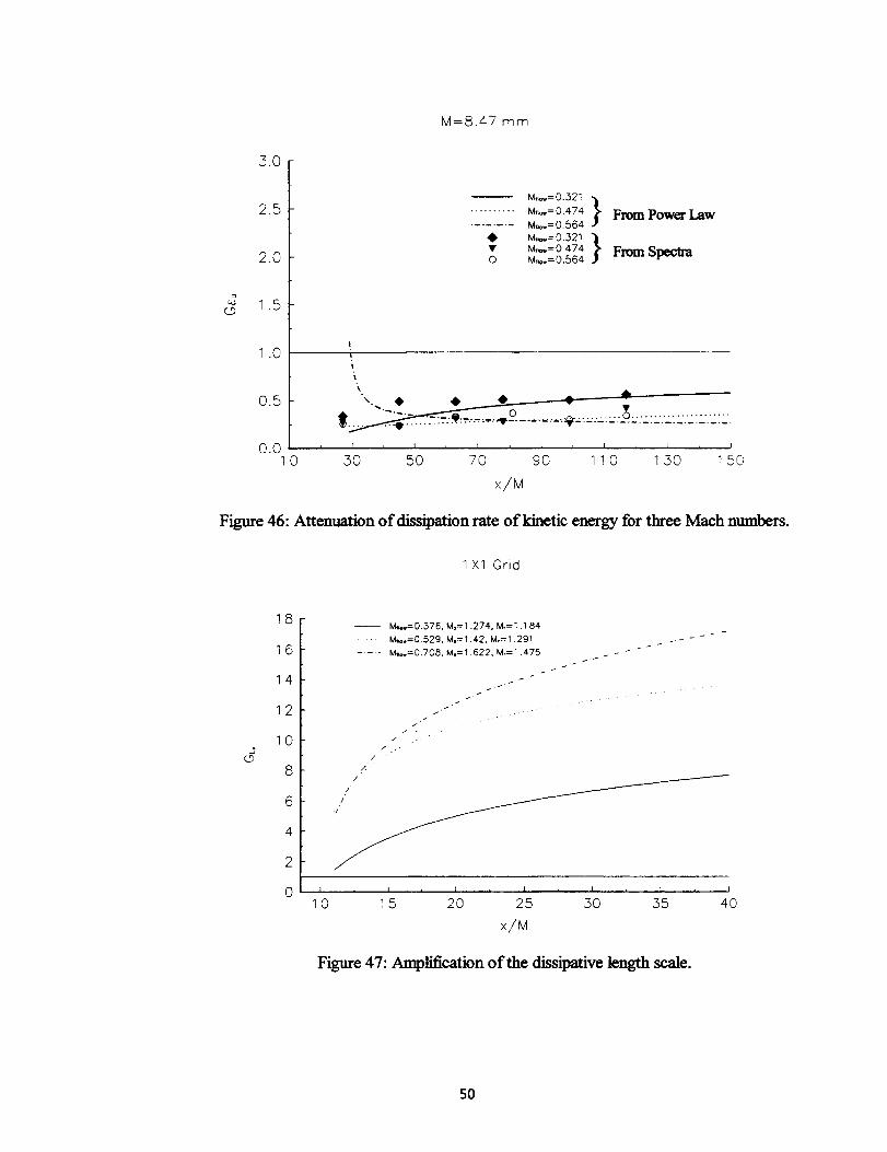
M=8.47 mrrl

5.0

o

2.5

2.0

1.5

1.0

0.5

M_ =0 321 }.......... M,L_,=O. 474 From Power Law........ M,_,,= 0.564

0 M,.,,= 0.321 }• M f_=O 474 From Spectra0 M_,=0.564

|

I

i

_. _ • • __.. ..... _2 ..........."_.... _:7.'.' ..... _._:u,'_.Z.'£:L.'L:2"./:L'._[_.

0 . 0 I l I 1 I f I { I I i _ I

1 0 50 50 70 90 11 0 1 50 1 50

×/M

Figure 46: Attenuation of dissipation rate of kinetic energy for three Mach numbers.

1 X1 Grid

_J

(_9

18

16

14

12

10

8

6

4

2

0

-- M_,,=0.376, M,=1.274, M,=I .1 84

...... M,_.=0.529, M,=1.42, M,=I .291

..... M,..=O 708 M,=I 622 M=I 475

/ , -

/ ../.

z

f

/

I i I i _ i I i I , I

1 0 1 5 20 25 30 35

×/M

Figure 47: Amplification of the dissipative length scale.

r

4O

5O

1xl Grid

1.8

1.7

1.6

1.5

1.4

1...%

1.2

1.1

1.0

M*k,_= 0.376. M,=1,274, M,=I .I 84

M.o._0.529, M,=1.42. M,=1.291

M,.,,..=0.708, M.=1,622. M,=1.475

I i I l I

0 1 5 2O 25

x/M

30 35P

40

Figure 48: Amplification of the viscous length scale.

1 xl Grid

d

2

@0

-- M_.=0.376, M.=1.274. M.=1.184. >,.

k&,,..=0.529, Mo=1.42, M,=1.291. X.

-- - M,',o.=0.708, M.=1.622, M,=I 475,

• M,_,=0.376, M.=1.274, M.= 1,184, _.

• M,.,.,=O 529, M.=I .42. M,= 1.291. _.

0 M,_.=O 708. M.=1.622. M.=I 475, l,

'/

o g

, I i I , I , I

1 0 20 50 40

x/M

Figure 49: Amplification of the Taylor's microscale.

51

Amplification of Pressure for various Grid SizesP4/P! =7.46

4--4--- 4 x 4 GRID....A... 2x2GRID•-.e-.- lOX 10 GRID---_-- Honkon et 01.(1 993)

3f , • .

2 _ ...... • ....• t ....... l ........... i .......... •

• "'"-.&. .... •

I s I • I I = I i I I |

0 0 1O0 200 300 400 500 600 700

x/M

i

8OO

Figure 50: Amplification of wan pressure fluctuations for various grids.

52

I

Figure 5 l a: Incompressible shear layer growth.

I

M ,

I ..........

Xo

Figure 51 b: Compressible shear layer growth.

53

REPORT DOCUMENTATION PAGE Po_nApp_o.,dOMB No. 0704-0188

Public reporting burden for this collection of information is eslJrnated to average 1 hour per resl_nse, including the lime for reviewing instructions, searching existing data sources,_atharing and maintaining the data needed, end completing and reviewthg the colection of information. Send comments regarding this burden estimate or any other aspect of this:ollection of informalion, including suggestions for recluc_ng this burden, to Washington Headquarters Services. Directorate for Inlormation Operations and Reports, 1215 JeffersonDavis Highway, Suite 1204, Arlington, VA 22202-4302, and to the Office of Management end Budget, Paperwork Reduction Project (0704-0188), Washington, De 20503.

1. AGENCY USE ONLY (Leave blank) 2. REPORT DATE 3. REPORT TYPE AND DATES COVERED

March 1998 Contractor Report

4. TITLE AND SUBTITLE 5. FUNDING NUMBERS

Studies of Shock Wave Interactions With Homogeneous and IsotropicTurbulence

6. AUTHOR(S)G. Brussels, J. Ague, C. B. Watkins, Y. Andreopoulos

7. PERFORMINGORGANIZATIONNAME(S)ANDADDRESS(ES)The City College of the City University of New YorkDepartment of Mechanical EngineeringNew York, NY 10031

9. SPONSORING/MONITORING AGENCY NAME(S) AND ADDRESS(ES)

National Aeronautics and Space AdministrationLangley Research CenterHampton, VA 23681-2199

G NAG1-1590

WU 282-10-01-01

8. PERFORMING ORGANIZATIONREPORT NUMBER

10. SPONSORING/MONITORING

AGENCY REPORT NUMBER

NASAJCR- 1998-206948

11. SUPPLEMENTARY NOTES

Langley Technical Monitor: Dennis M. BushnellFinal Report

12a. DISTRIBUTION/AVAILABILITY STATEMENT

Unclassified-Unlimited

Subject Category 34 Distribution: StandardAvailability: NASA CASI (301) 621-0390

12b. DISTRIBUTION CODE

13. ABSTRACT (Maximum 200 words)

A nearly homogeneous nearly isotropic compressible turbulent flow interacting with a normal shock wave has beenstudied experimentally in a large shock tube facility. Spatial resolution of the order of 8 Kolmogorov viscous lengthscales was achieved in the measurements of turbulence. A variety of turbulence generating grids provide a widerange of turbulence scales. Integral length scales were found to substantially decrease through the interaction withthe shock wave in all investigated cases with flow Mach numbers ranging from 0.3 to 0.7 and shock Mach numbersfrom 1.2 to 1.6. The outcome of the interaction depends strongly on the state of compressibility of the incomingturbulence. The length scales in the lateral direction are amplified at small Math numbers and attenuated at largeMach numbers. Even at large Mach numbers amplification of lateral length scales has been observed in the case offine grids. In addition to the interaction with the shock the present work has documented substantial compressibilityeffects in the incoming homogeneous and isotropic turbulent flow. The decay of Mach number fluctuations wasfound to follow a power law similar to that describing the decay of incompressible isotropic turbulence. It wasfound that the decay coefficient and the decay exponent decrease with increasing Mach number while the virtualorigin increases with increasing Mach number. A mechanism possibly responsible for these effects appears to bethe inherently low growth rate of compressible shear layers emanating from the cylindrical rods of the grid.

14. SUBJECT TERMS

Shock interaction; Turbulence amplification; Turbulence scale change

17. SECURITY CLASSIFICATION

OF REPORT

Unclassified

NSN 7540-01-280-5500

18. SECURITY CLASSIFICATION

OF THIS PAGE

Unclassified

19. SECURITY CLASSIFICATION

OF ABSTRACT

Unclassified

15. NUMBER OF PAGES

5816. PRICE CODE

A04

20. LIMITATION

OF ABSTRACT

Standard Form 298 (Revo 2-89)Prescribed by ANSi Std. Z39-18298-102

54