study of a night sky radiator cooling system utilizing ... · pdf filea thesis presented in...
TRANSCRIPT

Study of a Night Sky Radiator Cooling System Utilizing
Direct Fluid Radiation Emission and Varying Cover Materials
By
William Overmann
A Thesis Presented in Partial Fulfillment of the Requirements for the Degree
Master of Science
Approved November 2011 by the Graduate Supervisory Committee
Patrick Phelan Chair
Robert Taylor Steven Trimble
ARIZONA STATE UNIVERSITY
December 2011
i
ABSTRACT
As the demand for power increases in populated areas so will the demand for water
Current power plant technology relies heavily on the Rankine cycle in coal nuclear and solar
thermal power systems which ultimately use condensers to cool the steam in the system In dry
climates the amount of water to cool off the condenser can be extremely large Current wet
cooling technologies such as cooling towers lose water from evaporation One alternative to
prevent this would be to implement a radiative cooling system More specifically a system that
utilizes the volumetric radiation emission from water to the night sky could be implemented This
thesis analyzes the validity of a radiative cooling system that uses direct radiant emission to cool
water A brief study on potential infrared transparent cover materials such as polyethylene (PE)
and polyvinyl carbonate (PVC) was performed Also two different experiments to determine the
cooling power from radiation were developed and run The results showed a minimum cooling
power of 337 Wm2 for a vacuum insulated glass system and 3757 Wm2 for a tray system with a
maximum of 9861 Wm-2 at a point when conduction and convection heat fluxes were considered
to be zero The results also showed that PE proved to be the best cover material The minimum
numerical results compared well with other studies performed in the field using similar techniques
and materials The results show that a radiative cooling system for a power plant could be feasible
given that the cover material selection is narrowed down an ample amount of land is available and
an economic analysis is performed proving it to be cost competitive with conventional systems
ii
Thanks to my friends and family for putting up with me
iii
ACKNOWLEDGMENTS
Dr Patrick Phelan provided much input and support throughout the process of this thesis
Many of my fellow lab colleagues provided valuable insight and a helping hand including Rob
Jon Andrey Mark W Mark M Brent Carlos Erin Wei and Aziz as well as others Thank you to
all involved
iv
TABLE OF CONTENTS
Page
LIST OF TABLES vi
LIST OF FIGURES vii
NOMENCLATURE ix
INTRODUCTION 1
Motivation 1
Objective 2
Potential for Utilities 3
Background 4
Methodology 6
Atmospheric Window 7
PLANCKrsquoS LAW 9
EFFECTIVE NIGHT SKY 12
INFRARED ANALYSIS 14
Sample Materials 14
Infrared Camera Overview 14
IR Camera Experimental Setup and Process 15
IR Camera Results 15
FTIR Spectrometer 17
FTIR Results 19
RADIATIVE COOLING EXPERIMENTAL SETUP 24
Date amp Location 24
Vacuum Insulated Glass (VIG) 26
Tray Experiment 28
MODEL 32
EXPERIMENTAL RESULTS 38
v
Metric for Analysis 38
VIG Results 39
Tray Radiator Results 42
Experimental Uncertainty 46
DISCUSSION amp CONCLUSION 47
FUTURE WORK 49
REFERENCES 51
vi
LIST OF TABLES Table Page
1 Table 1 Summary of published sky radiator data 6
2 Table 2 Materials selected for IR 14
3 Table 3 Container radiation areas and water volumes 26
4 Table 4 Experiment data and calculations at ambient and water crossover point 45
vii
LIST OF FIGURES Figure Page
1 Setup of air cooling radiator room (Michell amp Biggs 1979) 1
2 Diagram of conventional aluminum radiator cooling system 2
3 Flowchart for experimental process 7
4 Percent transmittance of the Earthrsquos Atmosphere (Short) 8
5 Blackbody emissive power over a broad light spectrum (Carvalho 2010) 10
6 Blackbody emissive power at relevant cooling temperatures with the orange bar crossing at
the maximum values of E 11
7 FLIR ThermoCAMreg S60 (American Infrared) 15
8 IR camera test setup with glass slide sample 15
9 FLIR camera image of plastic wrap PVC 16
10 FLIR camera image of painterrsquos roll polyethylene 16
11 FLIR camera image of white trash bag polyethylene 17
12 FLIR camera image of glass slide 17
13 Diagram of ATR evanescent wave (Technologies 2010) 18
14 Nicolet FTIR spectrometer with Smart Orbit accessory (Universitat Politecnica de
Catalunya - Barcelona Tech 2011) 19
15 Selected materials from FTIR analysis 20
16 Extinction Coefficients of selected materials 23
17 Transmittance of selected materials with given thickness in Table 2 23
18 Experiment Location 24
19 CR23X Microloggerreg for Data Acquisition with attached thermocouples 25
20 Initial setup with 020A VIG fillers (foreground) and 70F VIG fillers (background) 27
21 Tray night sky radiator with white polyethylene cover 29
22 Diagram of tray experiment setup 30
23 Tray experiment setup 31
24 Diagram of the radiator model as a resistance network 33
viii
Figure Page
25 Theoretical model using ASU weather station temperature data from 1028-292011 37
26 VIG experimental data from 918-192011 where initial ambient temp gt water temp 40
27 VIG experimental data from 106-72011 where initial ambient temp ~ water temp 41
28 VIG experimental data from 107-82011 where initial ambient temp lt water temp 42
29 Tray experimental results of a clear PE cover to a white PE cover Run on 1025-26 43
30 Tray experimental results where the clear PE is covered with an opaque board eliminating
radiation Run on 1030-31 44
31 Tray experimental results comparing a clear PE cover to a black aluminum foil cover 45
ix
NOMENCLATURE
A area [m2]
co speed of light in a vacuum [ms]
cp specific heat at constant pressure [JkgK]
E emissive power [Wm2]
rate of thermal and mechanical energy transfer [W]
h convective heat transfer coefficient [Wm2K]
h universal Planck constant [Js]
I radiation intensity [Wm2sr]
k Boltzmann constant [JK]
q heat transfer rate [W]
qrdquo heat flux [Wm2] Rdarr atmospheric downwelling thermal radiation [Wm2]
T temperature [oC]
t time [s]
V volume [m3]
x y z rectangular coordinates [m]
Greek Symbols
η wavenumber [cm-1]
ρ density [kgm3]
λ wavelength [microm]
ε emissivity dimensionless
σ Stefan-Boltzmann constant [Wm2K4]
Subscripts
b blackbody
dp dew point
db dry bulb
rad radiation
x
st stored
sur surroundings
1
INTRODUCTION
Motivation
Radiative cooling has been occurring from the beginning of time Objects and areas give
off heat in the form of radiation because of simple laws of nature The desert is a prime example of
radiative cooling and how effective it can be Deserts in the southwest United States can reach
temperatures over 43 degrees Celsius during the day while at night the temperature can reach
around 16 degrees Celsius lower
Current radiative cooling techniques involve not only radiation but conduction and
convection as well Typically the fluid in the system is either water or air In systems with air as
the fluid a radiator is placed on top of the area being cooled The warm air rises and is transferred
through convection to a metal radiator typically made of aluminum (Michell amp Biggs 1979) The
heat then conducts to the other side of the metal and is radiated to the night sky This type of setup
can be seen in Figure 1 It should be noted that the term night sky relates to the effective sky
temperature Tsky which is based upon conditions in the atmosphere such as cloudiness and
moisture content The temperature can reach as low as 230 K (Incropera Dewitt Bergman amp
Lavine 2007) An expression for Tsky will be discussed later in the paper
Figure 1 Setup of air cooling radiator room (Michell amp Biggs 1979)
2
All radiators have a working fluid and often times that fluid is water Typically piping is
used to remove heat from a specified area by transferring heat to the water and then the water
flows to the radiating portion of the system Again the radiator is typically aluminum and the heat
is transferred to allow for the aluminum to radiate heat to the sky as shown in Figure 2
Figure 2 Diagram of conventional aluminum radiator cooling system
The aluminum can be covered in a material such as black paint to create more of a black
body effect during radiation resulting in higher emission (Kimball 1985) To reduce heat gain
from convection cover materials are placed over the top of the radiator and the sides are built
higher to create an air gap between the radiator and cover Materials such as polycarbonate and
polyethylene are used because they can be fairly cheap and have a high transmittance in the ideal
wavelength range (Ali Taha amp Ismail 1995) The ideal wavelength range will be discussed
further in the sections covering atmospheric radiation and Planckrsquos Law
Objective
Current radiative cooling techniques involve a minimum of three modes of heat transfer
From the example above the three heat transfer modes are convection from air to metal
conduction through the metal and finally radiation to the sky Implementing a system that directly
radiates heat from the fluid removes conduction through metal from the process as well as the
metal from the system A system with a material that has high transmittance in the proper infrared
(IR) range such as polyethylene (PE) or polyvinyl chloride (PVC) can allow the water to directly
radiate heat to the night sky This would decrease the cost of a large radiator system and
potentially make the system more efficient due to avoiding an extra mode of heat transfer The
objective is to design and build experiments that determine the cooling power of a direct fluid
3
radiative system Comparisons are then made to current radiant cooling technologies and the
practicality of the system is determined
Potential for Utilities
Engineers can utilize this radiative cooling technique to cool homes warehouses
factories office buildings and even power plants More specifically to power plants radiation can
be a useful method for cooling condensers The water needed to cool a condenser typically has a
change in temperature of 10 oC which is not an extremely high value for a radiative system to
achieve (Culp 1991) The majority of current cooling technology utilizes water and consists of
cooling towers as well as capturing flowing water from rivers and streams for cooling There are
also plants that use dry cooling (convection with air) and it should be noted that they are not as
efficient as wet cooling systems and ultimately lead to lower overall plant efficiencies (El-Wakil
2002)
The prominent methods of cooling condensers using water are single-pass cooling from
rivers and streams single-pass cooling from artificial ponds and cooling towers (Culp 1991)
These methods have their own drawbacks Single pass cooling from rivers and streams while very
efficient causes thermal pollution that can negatively affect the wildlife in the flowing rivers and
streams Cooling towers and artificial cooling ponds are effective based on the principal of
evaporation which consequently means there needs to be some amount of make-up water each
time the water cycles through Evaporation can result in a 1 to 15 loss of water for every
cycle (El-Wakil 2002) This may not seem like a significant amount but an example with
quantitative values may make this more eye opening Consider a 1000 MW power plant that
utilizes wet cooling towers These cooling towers circulate roughly 49520 Ls-1 of water In a hot
climate such as the Southwestern United States evaporation losses turn out to be around 631 Ls-1
of water (El-Wakil 2002) If this power plant is running at full power for 12 hours the loss of
water due to evaporation is 2726 million liters And there will be more water lost from
evaporation during the other 12 hours the plant runs although not at full power
One potential solution for power plant cooling issues in areas where water is a precious
resource is a radiative cooling system Instead of using dry or wet cooling towers a field of
4
radiators could be used to dissipate the heat to the sky at nighttime and with further research
potentially even during the daytime
Background
There have been many publications on radiative cooling Unfortunately there has not
been a break through formula or method for radiative cooling that has caught on and made it to the
marketplace However there are many promising ideas in the field and they are discussed below
Cooling buildings via radiative transfer is a concept that has been studied for years One
study conducted an experiment that compared two huts identical in structure but with different
roof coverings (Michell amp Biggs 1979) One hut was built with a steel roof that was painted with
a specific white coating to act as a selective surface coating which reflected certain wavelengths
and emitted other wavelengths The other hut roof was made of aluminum and given a special
coating to make it absorb and emit within the appropriate atmospheric window of 8 to 13 microm (For
a better understanding of the atmospheric window see the section Atmospheric Radiation) The
experiment was run at night and the results showed that the roofs yielded similar cooling
performance and achieved 22 Wm-2 overall in radiative cooling power The actual cooling was
higher but convection losses contributed to the decrease in cooling power More importantly this
publication found that there was little difference between a blackbody radiator and a selective
surface radiator
Another method of cooling buildings utilizes a small pond on the rooftop to collect the
heat that has risen inside the building (Erell amp Etzion 2000) The heat can then be directly
radiated from the pond or it can be run through a system of fabricated radiators An experiment
with this method used three commercially available solar collectors with some modifications to
perform as radiators Water from a roof pond was circulated through the collectors during the
nighttime and inlet and outlet temperatures were recorded The experiment did not explicitly show
temperature loss from radiation but it can be inferred from data that showed a 15 oC increase in
ambient temperature while the fluid temperature only rose between 005 oC to 04 oC over the
same period of time While this publication did not provide astonishing results it did reveal that
5
coupling night time radiators with daytime solar collectors is within the realm of possibility and
should be studied further
One of the more interesting concepts of radiative cooling is the application of a radiator
for cooling to the sky during the daytime The issue with this concept is that trying to keep
incoming radiation from heating up the radiator is extremely difficult Proper selective surface
materials are needed so that an atmospheric window will only allow certain wavelengths to
transfer This is realized theoretically through Planckrsquos Law which will be discussed later One
publication detailed an experiment that utilized a radiative cooling system for air for 24 hours in a
location near the equator (Nilsson amp Niklasson 1995) The radiators were insulated boxes with
heaters built in and utilized various covers that were shown to have high reflectance to solar
wavelengths and high transmittance in the infrared range All covers were varied in thickness The
results showed that a cover containing zinc sulfide (ZnS) which happened to be the thickest was
able to perform cooling over 19 hours of the day and allowed for the least amount of heating
around the middle of the day at only 72 Wm2 However the thinner covers were able to make up
for this by cooling more effectively during the nighttime hours Even though the ZnS cover
successfully cooled over 19 hour of the day its modified selective surface properties mean that it
would be very expensive to produce and therefore not currently feasible Unfortunately the
publication did not mention the exact price
Other studies have been done to evaluate the effect of a flowing system for cooling water
via radiation One experiment that was run used a gravity-fed water flowing system (Ali Taha amp
Ismail 1995) The water was run through parallel plates with the top plate being the radiator made
of aluminum and painted black The radiator was covered with different types of polyethylene to
prevent convective losses The system with the thinner polyethylene cover had an average cooling
power of 327 Wm2 during the nighttime hours The authors also concluded that flowing systems
were more efficient than stagnant cooling systems for two reasons higher convective resistance
between plate and water when not flowing and the inlet water temperature is warmer relative to
the plate than the stagnant water
6
In a similar experiment solar collectors were used to alternately work as radiators during
the night (Matsuta Terada amp Ito 1987) To make this work the cover was made of a spectrally
selective surface The publication claimed a cooling radiation flux of 51 Wm2 on a clear night
while still achieving 610 Wm2 of solar collective flux in good conditions This study gives
promise to the concept of having a solar thermal collector during the day act as a sky radiator
during the night thus making use of all 24 hours in a day
One final publication to mention also backs up the claims made by Matsuta et al An
experiment was performed testing a panel made for both daytime solar collecting and nighttime
radiation cooling (Yiping Yong Li amp Lijun 2008) The novel part of this experiment was that
the collectorradiator was designed as a structural element as well and can be integrated into the
building as a support More importantly the experiment resulted in a cooling capacity of 50 Wm2
with a polyethylene or polycarbonate cover and 47 Wm2 without any cover A summary of the
results found from the publications mention can be seen in Table 1
Table 1 Summary of published sky radiator data
Author(s) Year Description Result Michell amp Biggs 1979 Two huts with different material radiators 22 Wm2 Matsuta et al 1987 Solar collectorssky radiators 51 Wm2 Ali et al 1995 Gravity fed aluminum radiator 327 Wm2 Yiping et al 2008 Model of solar collectorsky radiator 50 Wm2 Nilsson amp Niklasson 1995 Box radiators with daytime cooling 19 hours of cooling
Methodology
A simple order was used for the structure of the experiments in this thesis and can be
seen in the flow chart shown in Figure 3 Once the general topic of radiation was chosen the
concept of using direct fluid emission for cooling was selected as a specific area of study The first
step was to determine the materials to be used for the covers of the radiators A simple experiment
analyzing different materials with an infrared camera was performed These materials were
narrowed down to the ones that showed promise for being the most transparent in the infrared
wavelengths of light The selected materials PVC and two different PEs were analyzed with a
Fourier Transform Infrared (FTIR) spectrometer and the top two materials both PEs were used
7
for the experiments The first experiment run was on a small scale and involved vacuum insulated
glass (VIG) cylinders filled with water This experiment was run to determine if the concept of
direct radiation emission from a fluid was feasible Once the concept was validated the two
chosen polyethylene materials were used as covers in the tray experiments which most closely
simulated a scaled sky radiator Finally the best cover material was compared to a conventional
metal covered radiator using the same tray experimental setup
Figure 3 Flowchart for experimental process
Atmospheric Window
Due to certain physical properties of the atmosphere radiating to the sky is possible An
atmospheric window exists between the wavelengths of 8 and 13 microm This atmospheric window
means that atmospheric radiation emission and absorption are very low compared to other
wavelength ranges Because these are so low transmittance of thermal radiation can be very high
This can be seen in Figure 4 Wienrsquos Displacement Law which will be discussed further in the
paper shows that the peak radiation emission occurs around 10 microm because of the correlation
where objects on Earth typically emit radiation between 250 and 320 K (Mills 1999) However
cloud cover can hamper the effect of radiation Therefore dry climates with minimal pollution
would be ideal for the radiator cooling system proposed in this thesis
8
Figure 4 Percent transmittance of the Earthrsquos Atmosphere (Short)
9
PLANCKrsquoS LAW
Radiation plays a role in the heating and cooling of everything in the universe Every
object radiates over a spectrum of wavelengths but will emit a maximum amount of radiation at a
certain wavelength that is related to its current temperature The relation between the wavelength
and temperature is called Planckrsquos Law Planckrsquos Law can be seen in Equation 1 (Incropera
Dewitt Bergman amp Lavine 2007)
2 1 (1)
where Iλ b is the blackbody spectral intensity λ is the wavelength in a vacuum T is the
temperature the universal Planck constant is h = 6626x10-34 Js the Boltzmann constant is k =
1318x10-23 JK-1 and the speed of light in a vacuum is co = 2998x108 ms-1 Sometimes Planckrsquos
Law is written in terms of spectral blackbody emissive power Eλ b
(2)
A plot of Eλ b versus λ can be seen in Figure 5 Incropera et al noted that the distribution has
important characteristics Those characteristics are the following
1 the emitted radiation varies continuously with wavelength 2 at any wavelength the
magnitude of the emitted radiation increases with the increasing temperature 3 the
spectral region in which the radiation is concentrated depends on temperature with
comparatively more radiation appearing at shorter wavelengths as the temperature
increases 4 a significant fraction of the radiation emitted by the sun which may be
approximated as a blackbody at 5800 K is in the visible region of the spectrum In
contrast for T less than or about equal to 800 K emission is predominantly in the
infrared region of the spectrum and is not visible to the eye (Incropera Dewitt Bergman
amp Lavine 2007 p 737)
This last characteristic is very important to the work of this thesis
10
Figure 5 Blackbody emissive power over a broad light spectrum (Carvalho 2010)
As stated earlier the degree of temperature change from inlet to outlet of the cooling
water will only be about 10 oC Assuming that the water drawn up to enter the system is at ambient
temperature the range of temperatures can be estimated to be between 50 and 100 oF which
converts to a range of 283 K to about 311 K From these temperatures the potential wavelengths
that the water will radiate at were determined To find these wavelengths Wienrsquos Displacement
Law needs to be taken into account The formula is
(3)
where C3 = 2898 micromK and is called the third radiation constant (Incropera Dewitt Bergman amp
Lavine 2007) For a temperature of 283 Kelvin the maximum emissive power is at a wavelength
of 102 microm Water at a typical room temperature of 298 K has a maximum emissive power at 97
microm and if water were at 311 K it would have a maximum emissive power at 93 microm Figure 6
shows the blackbody emissive power for a range of temperatures relevant to the radiant cooling
system discussed in this thesis The figure is the graphical interpretation of Planckrsquos Law
formulated by Matlab code (Spetzler amp Venables 2004) It should be noted that the cover used in
11
the system must have a high transmittance in the wavelength range of 9 to 11 microm to have the
highest possible emissive power transferred
Figure 6 Blackbody emissive power at relevant cooling temperatures with the orange bar crossing
at the maximum values of E
12
EFFECTIVE NIGHT SKY
An approximate net rate heat transfer equation for radiation can be given as (Incropera
Dewitt Bergman amp Lavine 2007)
$ amp()$+ )$ (4)
where qrad is the radiation heat transfer from the surface in W σ = 5670x10-8 Wm-2K-1 is the
Stefan-Boltzmann constant ε is the emissivity of the source A is the area of the emitting source in
m2 Tsource is the temperature of the source in K and Tsur is the temperature of the surroundings in
K Analyzing this equation it becomes clear that there are many ways to increase qrad A larger
surface area for radiating or a higher emissivity can increase the heat transfer rate The other way
to increase qrad is to achieve a large difference between the temperature of the source of radiation
and the temperature of the surroundings that are receiving the radiation (∆T) Buildings and
objects are typically at ambient temperature or may even be above if they have stored some heat
due to being a large thermal mass and are not good for creating large ∆Ts To cool below ambient
a large heat sink is necessary That heat sink is the night sky
The equivalent night sky temperature or effective night sky temperature is somewhat
unclear in the scientific community and has various models that try to predict it Perez-Garcia
provides the following for a definition
A simple model for the description of the general radiation budget between the
atmosphere and the ground allows to assess that in the absence of any other heat transfer
mechanism the temperature of an ideal radiator in equilibrium with the sky could reach
the value of the so called equivalent sky temperature or effective sky temperature Tsky
(Perez-Garcia 2004 p 396)
Tsky can be defined by the relation to the dry bulb temperature written as
(Perez-Garcia 2004)
)- (5)
where Tdb is the dry bulb temperature in K and ε is the sky emissivity which is a function of the
dew point temperature Tdp in oC A definition for the dry bulb temperature is the temperature that
is measured by a thermometer in a moist air environment (Moran amp Shapiro 2004) In other
13
words the air temperature people associate with when asking about the weather is the dry bulb
temperature
While Equation 5 is considered a standard differences in defining the night sky
temperature relate to the emissivity ε Multiple models exist for determining this value Perez-
Garcia takes four models and makes direct comparisons with experimental data in an attempt to
determine the accuracy of each model Of the four models presented the model by Brunt proved
to be the most accurate (Perez-Garcia 2004) However the Brunt model relies on parameters that
were calculated for different areas all over the world Unfortunately these parameters were not
given and they were not easily accessible The three remaining models were fairly similar in their
accuracy of determining the night sky temperature So for the sake of simplicity the model with
the least amount of inputs was chosen This model happened to be the one given by Berdahl and
Fromberg in 1986 This model was also cited in a publication that discussed experiments of
radiatively cooling a building using flat-plate solar collectors (Erell amp Etzion 2000) It should be
noted that the emissivity for both equations are for clear skies ie no clouds dust pollution etc
The emissivity for the night sky and day sky are
0123 0741 8 062 100lt (6)
- 0727 8 060 100lt (7)
where Tdp is the dew point temperature in oC (Perez-Garcia 2004) The night sky emissivity will
be used for the model to be calculated in this thesis while the daytime equation can be neglected
because all of the experiments will be run at night However if research of daytime cooling
progresses this would certainly be applicable
14
INFRARED ANALYSIS
Sample Materials
The sample materials to be used as a potential cover for the radiator tested using the IR
analysis were selected based on the general input from fellow engineers curiosity for certain
materials and a general notion that some plastics are good for IR transmittance Other factors that
played into the sample selections were price and availability at the local hardware store All
samples were tested with both the IR camera and the FTIR spectrometer regardless of the results
from the preliminary test with the IR camera The materials selected can be seen in Table 2
Table 2 Materials selected for IR
Material Thickness [microm] $m2 3M Transparency Film (sheets used for overhead projectors)
1140 381
Typical glass slide 10160 2871 Plexiglass (Non-glare Plaskolyte) 12700 3875 Clear painterrsquos sheeting [Polyethylene (PE)] 1270 041 Polyvinyl chloride (PVC) (plastic wrap) 254 007 White trash bag (PE) 254 010 Black trash bag (PE) 635 010 Light switch plate (thermoset plastic) 165100 3637
Infrared Camera Overview
As stated previously selecting potential cover materials to utilize in the experiments
depended on two factors cost and infrared transmissivity To determine the infrared
transmissivity two tests were conducted The first test involved using a FLIR ThermaCAMreg S60
thermal infrared (IR) camera shown in Figure 7 to quickly determine if materials selected showed
any signs of having high transmission in the IR wavelengths of light
15
Figure 7 FLIR ThermoCAMreg S60 (American Infrared)
IR Camera Experimental Setup and Process
A cap with a diameter of 0076 m and depth of 0019 m was filled with water from the
tap and placed in the microwave for 2 minutes on high The resulting temperature of the water was
hotter than the ambient and could easily be picked up by the IR camera Many of the material
samples were either not long enough or not strong enough to be able to lie across the cap so a
small holding template was made out of cardstock and placed on the lid The setup can be seen in
Figure 8 Each sample was placed on the setup and an infrared picture was taken
Figure 8 IR camera test setup with glass slide sample
IR Camera Results
The IR images that the camera provided showed that the PVC sample and the two
different PE samples had the highest transmissivity The captured images can be seen in Figure 9
Figure 10 and Figure 11 The square cutout of the cardstock can be seen due to the cardstockrsquos
16
low transmissivity The heated water is shown in a dark red to orange color while the area of the
sample PVC and PEs can be seen because of its slightly lighter orange color To contrast the
FLIR camera image of the glass slide sample can be seen in Figure 12 which shows low
transmission in the infrared light wave range
Figure 9 FLIR camera image of plastic wrap PVC
Figure 10 FLIR camera image of painterrsquos roll polyethylene
17
Figure 11 FLIR camera image of white trash bag polyethylene
Figure 12 FLIR camera image of glass slide
FTIR Spectrometer
The cover material samples were analyzed on a Fourier Transform Infrared (FTIR)
spectrometer with a wavelength range of 25 to 20 microm to determine IR properties particularly
transmittance The machine used was a Nicolet 6700 FT-IR spectrometer by the Thermo Electron
18
Corporation (Now Thermo Fisher Scientific) The spectrometer utilized the Smart Orbit which is a
single-bounce diamond attenuated total reflection (ATR) accessory ATR is a sampling tool that
sends an IR beam of light into a crystal with a large index of refraction The beam reflects from
the inside of the crystal creating an evanescent wave This wave enters the sample material that is
laid on top of the crystal at a right angle The evanescent wave loses some of its energy due to
absorption of the sample material while the remaining energy of the wave is sent back to the
detector The signal at the detector can then be converted into meaningful data such as the depth of
penetration From this absorbance and transmittance can be determined (Technologies 2010) A
diagram of how ATR works with a sample can be seen in Figure 13
Figure 13 Diagram of an ATR evanescent wave (Technologies 2010)
The FTIR spectrometer with Smart Orbit accessory can be seen in Figure 14 The
product configuration for the accessory was for the Nicolet Avatar and Nicolet Nexus Each
sample was first cleaned with isopropyl alcohol and the plate was cleaned with methanol To run
the test each sample was placed over the diamond crystal and held down with the pressure tower
that was hand tightened
19
Figure 14 Nicolet FTIR spectrometer with Smart Orbit accessory (Universitat Politecnica de
Catalunya - Barcelona Tech 2011)
The software the spectrometer used was Thermo Scientificrsquos Omnic package The
software required minimal setup Some important settings chosen were the following using 64
scans outputting the data in terms of transmittance and using a gain of 2 The 64 scans were
chosen due to unfamiliarity with the machine Sixteen scans would have been enough to gather a
reading of the material The gain of two was the default setting All other settings were kept at the
default settings Before testing each sample a background was collected This allowed for the
machine to compute the transmittance from the material and then display it in the correct terms
Each sample was tested three times using three different locations on the sample to provide an
average set of data
FTIR Results
The software provided a result for each test plotting the wavenumber cm-1 (x-axis)
against transmittance (y-axis) The data was transferred to Microsoft Excel and the
wavenumber η was converted to wavelength microm using the formula found in Equation 8 An
updated plot was then created
10000= (8)
20
The FTIR machine provided data to determine more specifically what materials were
suitable to test as cover materials Figure 15 shows the FTIR results for clear polyethylene
painterrsquos sheeting a white polyethylene trash bag and PVC plastic wrap All three of these
samples proved to be very transparent in the desired wavelength range with the two polyethylene
samples having a higher transmittance between 8 and 14 microm
It should be noted each set of data is an average of three samples from the FTIR
spectrometer Each sample was tested three times to display slight differences in testing conditions
due to the inability to apply the same amount of pressure with the clamp on the sample each time
Figure 15 Selected materials from FTIR analysis
Extinction Coefficients
The data from the FTIR spectrometer was used to calculate extinction coefficients for the
material tested This was useful because once an extinction coefficient is determined the
transmittance no longer only applies to a certain thickness but can be calculated at varying
thicknesses For simplicity Beerrsquos Law was applied to determine the extinction coefficients
Beerrsquos Law is written as
21
gt AB) (9)
where τη is the transmittance s is the thickness of the material and κη is the extinction coefficient
The subscript η denotes that it is a function of the wavenumber (Modest 2003) This can easily
be converted to wavelength by simply taking the reciprocal of the wavenumber
To find the extinction coefficients both values for the thickness and transmissivity were
needed The transmissivity values for the range of wavelengths were taken from the FTIR data
The thickness was found using equations from attenuated total reflection spectroscopy theory
This calculated thickness is called the effective path length (EPL) (Averett Griffiths amp
Nishikida 2008) Calculating the EPL requires looking at the effect of polarization on the
measurement from the FTIR spectrometer and therefore is dependent on certain properties of the
machine and setup The effect of polarization is split into two separate equations which are
C+) DEFGD1 DFHDG D (10)
C+ DEFG2FHDG DD1 DI1 8 DFHDG DJFHDG D (11)
where des is the effective thickness for perpendicular polarization dep is the effective thickness for
parallel polarization n21 is the ratio of the indices of refraction (n2n1) λo is the wavelength in a
vacuum θ is the angle of incidence of the inner surface of the diamond crystal n1 is the refractive
index of the diamond crystal and n2 is the refractive index of the sample (Harrick amp du Pre 1966)
The effective penetration is calculated as
C+ C+) 8 C+)2 (12)
Finally the EPL is given by
KL M N C+ (13)
where N is the number of reflections or bounces in the diamond crystal This EPL is then paired
with its respective wavelength in a vacuum λo and entered into Beerrsquos Law from Equation 9
(Technologies 2010)
22
The data from the FTIR was used to determine extinction coefficients for the PVC white
PE and clear PE It should be noted that the amplitude on the original data from the machine is not
accurate Looking back at Figure 15 the Transmittance is actually higher than 100 at certain
wavelengths This is the result of a focusing error within the machine where too much light is
reflected back into the detector due to a diverging parallel beam causing it to register a higher
intensity of light than is actually occurring (Young) To account for this a modification to the data
was made The highest transmittance value was determined for each material If that value was
higher than 1 the difference between the value and 1 was determined That difference value was
then subtracted from the other transmittances leaving the highest transmittance at a value of 1 The
modified transmittances were used in the Beerrsquos Law equation to calculate the extinction
coefficients
A plot of the extinction coefficients for the PVC clear PE and white PE can be seen in
Figure 16 Once the extinction coefficients were known the transmittance at all wavelengths was
calculated using the thickness of the material The thicknesses for the materials used for this thesis
can be found in Table 2 The actual transmittance for the materials can be seen in Figure 17 From
this figure it can be seen that the best option is the white polyethylene cover While it has
relatively the same extinction coefficients as the clear polyethylene itrsquos thickness of only 254 microm
makes it more transmissive than the 1016 microm clear PE The PVC is not appropriate for this
experiment because of its higher extinction coefficients and therefore a lower transmittance It
should be noted that each material shows an emissivity of 1 at some point in the plot ie the clear
PE has a transmittance of 1 between a wavelength of 4 and 5 microm This is due to the amplitude
error in the machine measurement as well as the modification that was made to the data
As Figure 17 shows the white polyethylene has the highest transmittance on average for
the three materials More specifically it has a value around 09 between the wavelengths of 8 and
13 microm Therefore the value for the transmittance of the cover in the model will be taken as 09
23
Figure 16 Extinction Coefficients of selected materials
Figure 17 Transmittance of selected materials with given thickness in Table 2
24
RADIATIVE COOLING EXPERIMENTAL SETUP
Date amp Location
The experiments took place between August and November of 2011 The experiments
were run on the rooftop of the Engineering Center F Wing on the Tempe Campus at Arizona State
University It should be noted that there were many objects and buildings in the surrounding area
and in the radiator field of view that could affect the radiative emission from the water and they
will be discussed later Figure 18 shows the layout of the rooftop and where the different
experiments were placed The reason that the experiments were in different locations was because
of the size of the setup and the proximity to an outlet for power The tray experiment was run
further away from the small room because the trays took up much more space than the glass
containers Also the location of the tray experiments helped reduce the shape factors of the
objects on the rooftop This was not considered as much of an issue with the glass containers
because it was only for validation
Figure 18 Experiment Location
Micrologger and Thermocouples
A Campbell Scientific CR23X Microloggerreg for Data Acquisition was used to measure
the temperatures of the water in the various containers as well as the ambient air Data collection
was performed by using the program PC200W version 41 This software allows the user to
monitor data in real time and collect data for further analysis with other software A Gigawarereg
USB-A to Serial DB9 connector was used to connect the CR23X Micrologger to a laptop
25
computer Five total thermocouples were used in the experiment The CR23X Micrologger setup
can be seen in Figure 19
Figure 19 CR23X Microloggerreg for Data Acquisition with attached thermocouples
Four Omega hermetically sealed tip insulated thermocouples were used for obtaining the
temperature of the various water samples Three of those thermocouples were type J and the other
was type K The thermocouples were 24 AWG stranded and 1 m in length Two different types
were used due to the limited supply of these thermocouples in the lab The thermocouples were
calibrated using the CR23X Micrologger while being submerged in ice water The temperatures
displayed were compared with the temperature measurement from a -5 oC to 30 oC Immersion
Thermometer by the Kessler Thermometer Corporation The results showed that the
thermocouples were only off by a maximum of 02 oC Originally the ambient air temperature was
measured using the reference temperature from the CR23X Micrologger But after a couple nights
of data collection this temperature was noticeably lower than recorded temperatures from weather
stations around the area This data was thrown out and the ambient air temperature was then
measured using a typical insulated type K thermocouple with an exposed junction which
produced much more accurate results This thermocouple was also calibrated in ice water with the
26
CR23X Micrologger and immersion thermometer During the experiment data was recorded
every two seconds This data was then averaged for a period of one minute The output data was
given in temperature every one minute
Vacuum Insulated Glass (VIG)
The experiment involved different vacuum insulated glass (VIG) inserts The original
idea came from the concept of a large Dewar flask This would eliminate the need to insulate the
sides Because Dewar flasks are very expensive older commercial vacuum flasks were the next
alternative Unfortunately due to vacuum flasks being out of date and relatively hard to find six
different flasks were purchased but consisted of four different types This was considered to be
acceptable due to the fact that this experiment was only used as a verification test for the larger
tray experiment
The first round of testing used two Aladdinreg VIC 020A fillers and two Thermosreg VIC
70F fillers The dimensions for these containers as well as containers used in latter experiments
can be seen in Table 3 The containers were placed in holes cut out in extruded polystyrene and
placed in a cardboard box as shown in Figure 20
Table 3 Container radiation areas and water volumes
Container 020A 040A 70F 72F Tray clear PE
Tray white PE
area [m2] 2819x10-3 5076x10-3 4774x10-3 4576x10-3 0344 0344
volume of water [m3] 25x10-4 37x10-4 30x10-4 37x10-4 12x10-2 17x10-2
27
Figure 20 Initial setup with 020A VIG fillers (foreground) and 70F VIG fillers (background)
The top portions of the containers were wrapped with reflective bubble wrap insulation
so that no glass was left exposed to the open air The 020A VIG containers were filled with 250
mL of water while the 70F containers were filled with 300 mL of water This left a distance of 2
and 3 inches of air between the water and the tops of the 020A and 70F containers respectively
The containers were covered with clear 4 mil (~100 microns) polyethylene painterrsquos sheeting To
keep the polyethylene attached rubber bands were placed around the covers The wrinkles were
smoothed out so that the water had a clear path to radiate to the sky Also shown in Figure 20 are
the thermocouples They were placed in the water by being bent over the edge of the container and
held down by the rubber band around the cover material
This setup was run multiple times with two different main conditions The first round of
experimenting started with water that was well below ambient temperature at the beginning of the
process The water in the containers was kept in a room with an average temperature of 27 degrees
Celsius while ambient was 37 degrees Celsius or higher The second experimental condition was
having the water in the containers start at ambient temperature This was done by placing the test
setup outside with a piece of cardboard covering the containers to prevent incoming radiation from
28
heating the water up or letting heat escape via radiation and cool the water down The cover was
then removed when the temperatures of the water were even with the ambient temperature
The next setup for the VIG containers involved plastic wrap to verify the results from the
FTIR analysis One of the 020A containers had the clear polyethylene removed and was replaced
with clear plastic wrap made of polyvinyl chloride (PVC) The tests run utilized all four
containers with the other three remaining the same as before The next series of tests involved
larger VIG 72F filler and medium sized 040A filler Both of these containers were filled with
approximately 370 mL which left a gap of approximately 2 and 3 inches from the top rim for the
medium and large containers respectively Both of these containers were covered with clear
polyethylene Another setup replaced the clear polyethylene cover with white polyethylene taken
from a trash bag The white polyethylene covered the 040A container
The overall goal of this experiment was to gain a sense of how successful an actual tray
radiator may be at radiating heat to the night sky The small containers were given different initial
conditions to determine if one the water could be cooled below ambient temperature by radiation
on a small scale and two to determine if different initial conditions affected the experiment in any
way It will be seen that the results of these experiments justified continuing the project by scaling
up the size of the radiators and simulating more closely the design of a potential commercial
radiator
Tray Experiment
Earlier in this thesis it was noted that one way to increase the rate of radiative heat
transfer is to increase the area being cooled The VIG containers have a radiation view area of
approximately 452 cm2 for the 70F 72F and 040A containers while the 020A containers have a
radiation view area of approximately 30 cm2 Presumably the experiments should scale up for
radiators with larger areas In order to provide experimental data to back this claim up two
fiberglass trays with a depth of approximately 2 inches and a total area of 0344 m2 were modified
into night sky radiators A modified tray can be seen in Figure 21 and a diagram of the entire tray
system can be seen in Figure 22 On each of the shorter ends of both trays a small hole with
diameter ~ 6 mm was drilled and an aluminum tube was fitted and bent up so that the top of the
29
tube was higher than the rim of the tray This was done to provide a way to submerge the
thermocouples in the water without having to seal them to the fiberglass Another hole of diameter
~ 25 cm was drilled to fit a PVC pipe on the same end as one of the aluminum tubes This was
built in for an easy access point to fill the system with water The two aluminum tubes and PVC
pipe were attached to the fiberglass tray using Loctitereg Professional Heavy Duty Epoxy Each
tube and pipe was also sealed with Polyseamseal reg Speed Seal Silicone Sealant to prevent water
leaking through any holes not completely covered with the epoxy
Figure 21 Tray night sky radiator with white polyethylene cover
30
Figure 22 Diagram of tray experiment setup
Each tray received a different cover One tray was covered with the clear polyethylene
painterrsquos sheet with a thickness of 101 microns The other tray was covered with white
polyethylene from a trash bag with a thickness of 25 microns Polyethylene is extremely difficult
to bond to other materials To achieve this 3Mreg Hi-Strength 90 Spray Adhesive was used
because itrsquos specifically designed for plastics Finally insulation was added to the trays to reduce
the effect of convection Two layers of one inch thick extruded polystyrene were added on the
bottom surface of the trays The outer walls were then covered with two layers of reflective
insulating bubble wrap Both the polystyrene and bubble wrap were attached using ACEreg Carpet
Tape Fiberglass and duct tape
Once the trays were fully modified they were filled with water Each tray was filled with
18 liters of water but this changed due to leaking in the system The white PE tray was estimated
to have 17 liters while the clear PE tray was estimated to have 12 liters The trays were filled up
near the top of the rim but a 001 m space was left for air to act as a barrier It should be noted that
the cover was not even with the edge of the tray but higher due to the flexible nature of the plastic
31
and the pressure from the air sitting on top of the water The same thermocouples and CR23X
Micrologger were used to take measurements Each tray utilized two thermocouples placed at
approximately the one third and two third marks on the tray to give a better idea of the overall
temperature of the water The setup for this experiment can be seen in Figure 23 A simple
variation was run with this setup as well In order to see how much of an effect convection had on
the system the experiment was run multiple times where the tray with the clear polyethylene was
covered with an opaque white poster board This was to effectively eliminate the heat loss from
the system due to radiation The last experiment involving these trays compared an aluminum
cover to the white polyethylene cover to determine if the direct fluid emission system can compete
with the conventional system The aluminum radiator was made by removing the clear
polyethylene from the other tray and adhering aluminum foil to the tray
Figure 23 Tray experiment setup
32
MODEL
A model was created to theoretically determine the effective cooling power of the
radiator The model was designed after the tray experiment using its dimensions as well as the
same materials and their properties A diagram of this model as a resistance network can be seen
in Figure 24 This diagram can be expressed by the equation
O PQCR SE FTU 8 PQCR SE infin 8 PQCR SE EWP 8 SEXY 8 FHCY 8 ZESSE[Y (14)
where qradw to sky is the radiation from the water to the sky qradw to infin is the radiation from the water
to the surroundings qradw to cover is the radiation from the water to the cover qtopR is the heat flux
calculated from the resistance network of the conduction through the air gap convection from the
cover to the surroundings and the radiation of the cover to the surroundings qsideR is the heat flux
from the resistance network of convection and conduction through the sides and qbottomR is the
heat flux from the resistance network of convection and conduction through the bottom The
radiation from the water to the cover can be neglected due to the very small difference in
temperature
33
Figure 24 Diagram of the radiator model as a resistance network
The model consists of 17 L of water inside the tray with dimensions of 0727 m by 0473
m for a total area of 0344 m The tray was 0048 m high The insulation on the bottom consisted
of 00508 m polystyrene with a conductive resistance Rcond of 4168 KW-1 and a convective
resistance Rconv of 0524 KW-1 The insulation on the sides consists of bubble wrap 00159 m
thick with Rcond of 0640 KW-1 and Rconv of 6369 KW-1 The air gap in between the water and the
cover is considered to be 001 m Because it is impossible to have forced convection between the
cover and water free convection was considered With some analysis using the Rayleigh number
and Nusselt number it can be seen that the air acts as a conductor with a thermal conductivity k
given for the appropriate temperature It should be noted that because the temperature range from
the experiment was from 300 K to 280 K an average temperature of air was used to determine
appropriate values That temperature was 293 K (20oC) for simplicity This was done only after
checking the equations utilizing associated values to this temperature with higher and lower
34
temperatures and seeing that the effect of using an average temperature was minimal From the
temperature of 293 K the following values were used for air density ρ = 1204 kgm-3 dynamic
viscosity micro = 182510-5 kgm-1s-1 thermal conductivity k = 002514 Wm-1K -1 and Prandtl
number Pr = 07308 (Ccedilengel 2007) The water also has an emissivity of 096 (Modest 2003)
Finally the cover was assumed to be polyethylene with a thickness of 254 microm an emissivity of
01 and a transmissivity of 09 from the FTIR analysis
It was assumed that the water can be taken as a lumped mass where the temperature is
constant throughout The experimental results can verify that the difference in temperature across
the water was rarely more than 05 oC From this lumped capacitance model a resistance network
was setup up to determine the heat moving in and out of the system Resistance networks utilize
the following equation
∆ΣY (15)
where ΣY is the sum of the resistances of each mode of heat transfer The first term found was the
heat transferred to the sky via radiation from the water written as
$^_)- ampgt( )- (16)
where σ is the Stefan-Boltzmann constant ε is the emissivity of the water τ is the transmissivity of
the cover A is the area of the water being radiated Tw is the temperature of the water and Tsky is
the same from the model mentioned in the Sky Temperature section of the thesis Along with
radiating to the sky the water also radiates to the surrounding area which was assumed to have a
temperature equal to the ambient temperature This expression is
$^_)$ ampgt(` )$ (17)
where Tsur is the temperature of the surrounding area and F is the shape factor computed by
analyzing the buildings and objects in the area It should be noted that the temperature of the
surrounding objects were assumed to be the same as the ambient temperature and may therefore be
also written as Tinfin F is determine by using the equation
12 SQD 1a aradicc 8 a SQD 1radicc 8 alt (18)
35
where F is the shape factor Y = ac and X = cb with a as the height b as the width and c as the
distance from the object (Modest 2003)
The cover also radiates to the sky and is represented by
$_)- ampd+$( )- (19)
where Tc is the temperature of the cover Its radiation to the surrounding objects can be neglected
because the temperature difference and emissivity are very small The terms for the conduction of
the water across the air to the cover the conduction across the cover and the convection from the
cover were lumped together in a resistance analysis written as
0d+$ )$e 1( 8 LT( 8 LT(f
(20)
where ha is the heat transfer coefficient of the air Lc is the thickness of the cover kc is the thermal
conductivity of the cover La is the characteristic length of the surface going through convection
(La = areaperimeter) and ka is the thermal conductivity of air The ha term was found by assuming
a value of 495 ms-1 for a wind speed taken from TMY3 data and finding the Reynoldrsquos number
which is
Y ghijk (21)
where Re is the Reynoldrsquos number uinfin is the wind speed x is the critical length and micro is the
dynamic viscosity From this equation the Nusselt number can be found using
Mhllll 2Mh 0664YKP (22)
where Mhllll is the average Nusselt number and Nu is the Nusselt Number Finally the Nussult
number can be plugged into the equation
Solving for h then gives ha This process is the same for finding the heat transfer coefficient for the
sides and bottom of the radiator as well Coupling the conductive and convective resistances
together gives the heat rate q for both the sides and bottom respectively
Finally the heat rates are totaled and set equal to the heat stored in the system shown by
Mh jT (23)
36
where V is the volume of water cp is the specific heat of water ΔT is the change in temperature of
the water and Δt is the time difference between each step To find the new temperature of the
water ΔT breaks up into
where Twold is the original temperature of the water and Twnew is the newly computed temperature
of the water The process was run with a Δt = 300 s over a 14 hour period Heat rates q were
calculated for each 300 s time step A 300 s time interval was considered adequate because the
ASU weather station data is given hourly therefore the 5 minute data is interpolated and not
entirely accurate with the 5 minute actual real time temperature data
The entire equation used for the model can be written as
The final result for the model can be seen in Figure 25 The plot shows the dry bulb
temperature the temperature change of the water the heat transfer rate and the sky temperature
The dry bulb temperature and dew point temperature used to calculate the sky temperature were
taken from the ASU weather station data center The data used was from October 28th through the
29th between 6 PM and 8 AM The heat flux at the crossover point (point when qconv and qcond = 0)
m gn ooS (24)
o p 0+^ (25)
gn p 0+^oS amp^gtd+$(3q )-r 8 amp^gtd+$(3` i8 iY301$ 8 Y30d+$ 8 Y30d1$ 8 Y3$d+$8 iY)1+)0s 8 Y)1+)0^$ 8 Y)1+)0d1$8 iY330s 8 Y330s 8 Y330d1$
(26)
37
is 7667 Wm-2 and occurs at 255 AM and the radiator efficiency (actual qradtotal divided by
qradideal) at this point is 092
Figure 25 Theoretical model using ASU weather station temperature data from 1028-292011
38
EXPERIMENTAL RESULTS
Metric for Analysis
To be able to compare the results from the conducted experiments the data collected
needed to be converted to a common metric A useful metric for this comparison is measuring the
heat flux per unit area This will also allow an easy comparison with the data reported in other
experiments as well Because the system is not flowing the only energy contained in the system is
the energy stored or the heat stored which can be written as
)3 )3 (27)
where )3 represents the energy stored and )3 represents the heat stored This will be the starting
point From here the heat stored can be represented as
)3 g ttS CjCUCu (28)
where ρ is the density cp is the specific heat vv3 is the time dependent temperature differential and
dxdydz is the combination differential of each direction (Incropera Dewitt Bergman amp Lavine
2007) Because the volume will not be changing
n CjCUCu (29)
where V is the volume Plugging this back into the heat stored equation gives
)3 gn ttS (30)
The temperature and time used for the analysis are simply the starting and ending temperatures for
each increment which results in
where ∆ is the difference in temperature and ∆S is the difference in time Finally the heat stored
term can be divided by the area to give the heat rate in terms of energy per unit area or Wm-2
giving
gn( p 0+^∆S (32)
)3 gn p 0+^∆S (31)
39
where A is the area of the surface that is radiating heat This qrdquo is the total heat flux of the system
which takes into account radiation convection and conduction Because qrdquo is not just the heat flux
due to radiation a specific value of the data will be looked This value is the crossover value
which is the point when the temperature of the water is the same as the temperature of the ambient
air At this point the difference in temperature is zero and therefore the heat flux can only be a
result of radiation
For the following results the density of water ρ was taken to be 1000 kgm-3 and the
specific heat of water was taken to be 4181 Jkg-1K-1 The areas of the containers and volume of
water are also needed to be able to perform the calculations These can be seen in Table 3
It should be noted that the heat flux values were calculated by averaging the one minute
interval values This interval was used because it was the interval that the CR23X Micrologger
retrieved data It contrasts to the model because the model uses 5 minute intervals of data While
the model could have used one minute intervals it was unnecessary because the temperature data
from the ASU Weather Station was only recorded on an hourly basis and therefore interpolation to
1 minute instead of 5 minutes would lead to the similar values for the heat flux
The tray experimental results make a comparison with the ideal heat flux due to radiation
This equation is
where the emissivity ε is for water The experimental results are divided by the ideal radiation
heat flux to give a radiation efficiency
VIG Results
This test was run multiple times to gather data for different initial conditions The
different initial conditions were having the water temperature initially warmer than the ambient
temperature the water temperature about equivalent to the ambient temperature and the water
temperature cooler than the ambient temperature All of these data presented is from experiments
that used clear PE which was considered the best because of durability
$1+p amp )- (33)
40
The experiment shown in Figure 26 had the initial condition of the ambient temperature
being higher than the water temperature The data shown reflects water from a 70F container The
heat flux was calculated to be 337 Wm-2 by averaging the one minute data over the entire period
This heat flux can only be from the effect of radiation because any other heat transfer mechanisms
would have increased the temperature of the water
Figure 26 VIG experimental data from 918-192011 where initial ambient temp gt water temp
The experiment shown in Figure 27 had the initial condition of the ambient temperature
being almost equal to the initial temperature of the water The data shown is from a 70F container
The heat flux for this experiment is 864 Wm-2 a figure much higher than the first experiment
discussed
41
Figure 27 VIG experimental data from 106-72011 where initial ambient temp ~ water temp
The final VIG experiment had the initial condition of the water temperature being higher
than the ambient temperature This data can be seen in Figure 28 Again this is data was taken
from the water temperature in a 70F container The total calculated heat flux from the data is 780
Wm-2
42
Figure 28 VIG experimental data from 107-82011 where initial ambient temp lt water temp
Taking these three experiments into account the water is certainly losing heat due to
radiation and therefore scaling up the experiment up to a larger radiator size with a more practical
shape is reasonable However the heat fluxes given all have other sources of heat loss and gain
affecting them both positively and negatively depending upon the temperature of the water in
relation to the ambient temperature When the water is warmer than the ambient air convection
helps decrease the temperature and makes the system more efficient and when the water is cooler
convection heats up the water negatively affecting the system
Tray Radiator Results
In these experiments the desired value is the heat flux due to radiation As shown in the
VIG experiments calculating the heat rate over the entire night gives the entire heat flux including
the effects of convection and conduction To eliminate these modes of heat transfer the portion of
the data where the ambient temperature is the same as the water temperature should be studied
This is because the temperature difference at these points is zero and therefore the convection and
conduction heat transfer is zero Due to the noise displayed in the ambient temperature data a ten
43
minute average was used to dampen the effect The value where the ambient temperature is the
same as the water temperature was selected and then the five data points before and after were
selected These correlating heat flux points of one minute of data were averaged to determine a
filtered value of the heat flux from radiation This value was then compared with the ideal heat
flux due to radiation from Equation 33
Figure 29 shows the tray radiators being exposed to the night sky and the water temperature started out higher than the ambient temperature Ultimately the heat flux of the entire period is not needed As stated previously the best point to estimate the heat flux due to radiation is at the crossover point of the water temperature and the ambient temperature For this set of data that crossover point has a heat flux of 6850 Wm-2 for the clear PE and 5635 Wm-2 for the white PE The radiation efficiencies at these points are 084 and 071 for the clear PE and white PE respectively All of this data along with other experimental data can be found in
Table 4 at the end of this section
Figure 29 Tray experimental results of a clear PE cover to a white PE cover Run on 1025-26
The data in Figure 30 displays an experiment run where the radiator with the clear PE
cover had the view of the night sky blocked by an opaque board This was done to show that the
temperature decrease when the temperature of the water is already below the ambient is caused
by radiation The water with the opaque board only decreases in temperature because of
44
convection and conduction The temperature of the water never drops below the ambient
temperature The heat flux at the crossover point for the white PE cover is 9861 Wm-2 and the
radiator efficiency is calculated to be 086
Figure 30 Tray experimental results where the clear PE is covered with an opaque board
eliminating radiation Run on 1030-31
The last figure of the section Figure 31 shows the data from the final tray experiment
run comparing the white PE cover to a conventional black painted aluminum cover The
temperatures of the water for both radiators follow each other closely The radiant heat flux at the
crossover point for the clear PE cover is 375 Wm-2 while the heat flux for the aluminum cover at
its crossover point is 5635 Wm-2 The radiator efficiency for the PE cover is 046 and for the
aluminum cover is 067
45
Figure 31 Tray experimental results comparing a clear PE cover to a black aluminum foil cover
Table 4 Experiment data and calculations at ambient and water crossover point
Date
PE
Cover
Time
[s]
Twater
[K]
Tinfin
[K]
Tsky
[K]
qrdquo rad total
[Wm -2]
qrdquo rad ideal
[Wm -2]
xyz||z~xyzz~1024-25 White 053 29800 29781 27880 4852 10456 046
1025-26 Clear 2230 29540 29520 27960 6850 8183 084
1025-26 White 020 29410 29414 27850 5635 7979 071
1027-28 Clear 2236 29053 29066 26915 6739 10218 066
1027-28 White 2236 29037 29066 26915 9078 10134 089
1030-31 White 2159 29491 29482 27181 9861 11460 086
1125-26 White 2334 28418 28414 26620 3757 8166 046
1125-26 Alum 2318 28474 28466 26630 5635 8408 067
46
Experimental Uncertainty
The root sum square method was used to determine the experimental uncertainty of the
data collected The three sources of error in the measurement came from the thermocouples the
CR23X Micrologger and the volume of the water The thermocouples had an error of 02oC when
first calibrated The CR23X operations manual states an error of 0025 when recording
temperature data between 0 and 20oC The error in the volume of water is due to leaks in the
system The error is +- 1 liter of water The assumed volume is 17 liters The root sum squares
method can be described as the following
h eh f 8 ehn f (34)
where uqq is the percent uncertainty in the heat rate which can be directly correlated to heat flux
uT is the uncertainty in the temperature and uV is the uncertainty in the volume For this analysis
the temperatures of 10 and 20oC will be considered because that is the range of temperatures in
which this experiment occurs At these selected temperatures the uncertainly from the Micrologger
can be neglected because it is much smaller than the uncertainty from the thermocouples At 20oC
the uncertainty percentage of qrdquo is 597 while the percent uncertainty of qrdquo at 10oC is 621 It
can be seen that the lower the temperature goes the higher the percent uncertainty becomes
47
DISCUSSION amp CONCLUSION
The vacuum insulated glass experiments showed that no matter the initial temperature of
the water relative to the ambient temperature radiation can create a heat flux that will cool the
water throughout the course of the night Even when the water temperature was below the ambient
temperature a radiant heat flux of 337 Wm-2 was achieved When considering the negative effects
of conduction and convection this number is certainly higher The VIG experiments that started
with a higher water temperature had much higher radiant heat fluxes with values around 80 Wm-2
While these cannot be directly attributed to radiation due to other heat transfer mode effects it is
clear that radiation helps decrease the temperature of the water and ultimately the experiment must
be scaled up to a more appropriate size such as the tray radiators
The data from the tray radiator experiments shows promise for the fluid emission
concept All the radiant heat fluxes at the crossover points have values higher than 35 Wm-2 with
the highest value of 9861 Wm-2 coming from the radiator with the white PE cover The white PE
cover also had the highest radiation efficiency of 086 The most important experimental results
are from the final experiment comparing the aluminum cover to the white PE cover The
aluminum cover outperformed the clear PE cover with radiant heat flux of 5635 Wm-2 compared
to 3757 Wm-2 These resulted in radiator efficiencies of 067 and 046 respectively The values in
Table 4 compare well to the model value of 7667 Wm-2 for the heat flux but do not compare as
well for the radiator efficiency of 091 Comparing these results to the ones achieved by other
researchers mentioned in the Background section these experiments were much more effective
One potential reason for the higher radiant heat flux may be due in part to geographic location and
therefore climate where the experiments took place Phoenix AZ is very dry which means it has a
lower dew point than most places This lower dew point directly affects the sky temperature by
causing it to be lower and thus creates a larger temperature difference between the water and its
heat sink the night sky Another potential reason for the differences may be because the system is
not flowing but without studying a flowing system this remains in question
An issue with these experiments and analysis originates from the ambient temperatures
First the thermocouple used was very sensitive and has quite a bit of noise during portions of the
48
varying experiments Essentially the two temperatures could cross multiple times due to the noise
in the ambient temperature data This created the need to average the one minute recorded heat
fluxes over a ten minute period Another issue is that the actual dew point temperature may be
slightly different than the dew point temperature data used from the ASU Weather Station This
may have resulted in a less accurate sky temperature
The cover materials used in the experiments all proved to be somewhat similar The two
PE covers provided very comparable results The white PE was chosen for comparison to the
aluminum cover because of the results from the FTIR analysis even though when directly
compared with the clear PE it was outperformed during one experiment as shown in Table 4
Potentially the clear PE cover could outperform the white PE if it were as thin as the white PE
However a system would need to be able to survive many years in the natural environment to be
cost effective Thicker polyethylene may need to be studied to determine if it can still be a good
infrared transmitter when made to be more durable
It is recommended that research in this area continue so that a more direct comparison to
the studies performed by other engineers and scientists can be made In particular the direct fluid
radiative cooling system described in this paper should be modified into a flowing system This
would give a more accurate depiction of whether or not a similar system could be ultimately
utilized in a power plant cooling process
49
FUTURE WORK
Based on the experimental data given in this thesis further studying the potential for
direct fluid radiative cooling would be recommended Many things could be done to improve upon
the experiments run The first step should be to better insulate the tray radiators While the VIG
containers were well insulated the trays were significantly affected by convection If possible
vacuum insulated trays would be ideal Based on the current shape that may not be possible A
potential variation to the project may be to add another cover over top of the radiator virtually
eliminating all but free convection This however would decrease the transmittance value
negatively affecting the radiative cooling value The convective heat gains to the system should be
measured against the radiative cooling losses to determine the wind speed at which point it would
be beneficial to add another cover
Testing for better cover materials would be another way to improve the project The
materials tested were not rigid Endurance may become an issue with the cover material due to a
lack of strength This is partly due to the reasoning that cheap materials mean a more economical
radiator It would also be worth testing materials found in nature such as BaF2 or AgBr known to
have high transmissivity in the appropriate IR range (Beamlines 2011) to see if radiative cooling
is improved
Once the ideal non-flowing system is determined the next step should be making the
system flow Many of the radiative cooling systems used for comparison in this paper were
flowing systems A direct comparison of a flowing system with a clear cover to a flowing system
using a metal radiator would be useful to determine which system would be more effective to cool
a fluid An economic analysis should also be performed to determine the cost of a system with
metal radiators compared to a system with IR transparent cover radiators
Another way to improve the radiative heat transfer is to increase the area being radiated
One possible way to do this is to tilt the radiators This would increase the area being radiated
while keeping the footprint the same A more in depth study of radiation shape factors would need
to be performed for this experiment One last idea to increase the radiation performance of the
system would be to utilize phase change materials in the water The goal would be to capture more
50
heat from the condenser by using materials such as waxes with a higher heat capacity than water
The waxes would be encapsulated and would transfer their heat to the water as the water is cooled
during the radiation process An alternative experiment to run that is similar to this would be using
nanofluids to see if the increased surface area from the particles increases the amount of cooling
from radiation
51
REFERENCES
Ali A H Taha I M amp Ismail I M (1995) Cooling of water flowing through a night sky radiator Solar Energy 235-253
American Infrared (nd) FLIR P0 FLIR P65 FLIR S60 FLIR S65 Infrared Sale Price or Rental Retrieved October 14 2011 from American Infrared httpwwwamericaninfraredcomProductDetailaspID=58
Carvalho M d (2010 July 7) Radiative Heat Transfer Retrieved October 24 2011 from Thermopedia (TM) BETA httpwwwthermopediacomcontent5491tid=104ampsn=132
Culp A W (1991) Principles of Energy Conversion New York McGraw-Hill Inc
El-Wakil M M (2002) Powerplant Technology New York The McGraw-Hill Companies Inc
Erell E amp Etzion Y (2000) Radiative cooling of buildings with flat-plate solar collectors Building and Environment 297-305
Incropera F P Dewitt D P Bergman T L amp Lavine A S (2007) Fundamentals of Heat and Mass Transfer 6th Edition Hoboken NJ John Wiley amp Sons Inc
Kimball B A (1985) Cooling performance and efficiency of night sky radiators Solar Energy 19-33
Matsuta M Terada S amp Ito H (1987) Solar heating and radiative cooling using a solar collector-sky radiator with a spectrally selective surface Solar Energy 183-186
Michell D amp Biggs K L (1979) Radiation Cooling of Buildings at Night Applied Energy 263-275
Moran M J amp Shapiro H N (2004) Fundamentals of Engineering Thermodynamics Hoboken NJ John Wiley amp Sons Inc
Nilsson T M amp Niklasson G A (1995) Radiative cooling during the day simulations and experiments on pigmented polyethylene cover foils Solar Energy Materials and Solar Cells 93- 118
Perez-Garcia M (2004) Simplified modelling of the nocturnal clear sky atmospheric radiation for environmental applications Ecological Modelling 395-406
Spetzler D amp Venables J (2004 February 18) Blackbody Radiation Retrieved October 6 2011 from Arizona State University httpvenablesasueduquantDavidSindexhtml
Universitat Politecnica de Catalunya - Barcelona Tech (2011 March) InfraredUV Spectroscopy - Center for Research in NanoEngineering Retrieved October 26 2011 from Universitat Politecnica de Catalunya - Barcelona Tech httpwwwupceducrneinfrastructureinfrared-uv- spectroscopy
Yiping W Yong C Li Z amp Lijun H (2008) Experiments on novel solar heating and cooling system Energy Conversion and Management 2083-2089
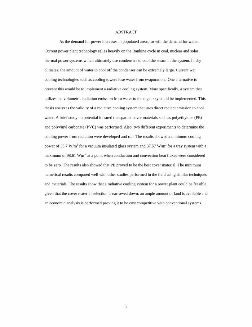
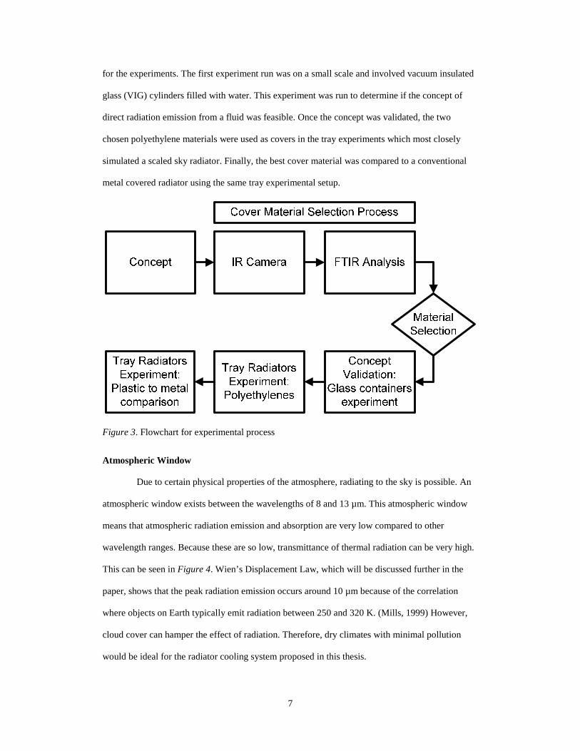
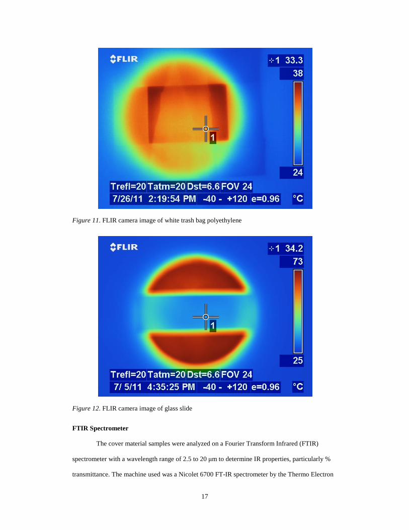
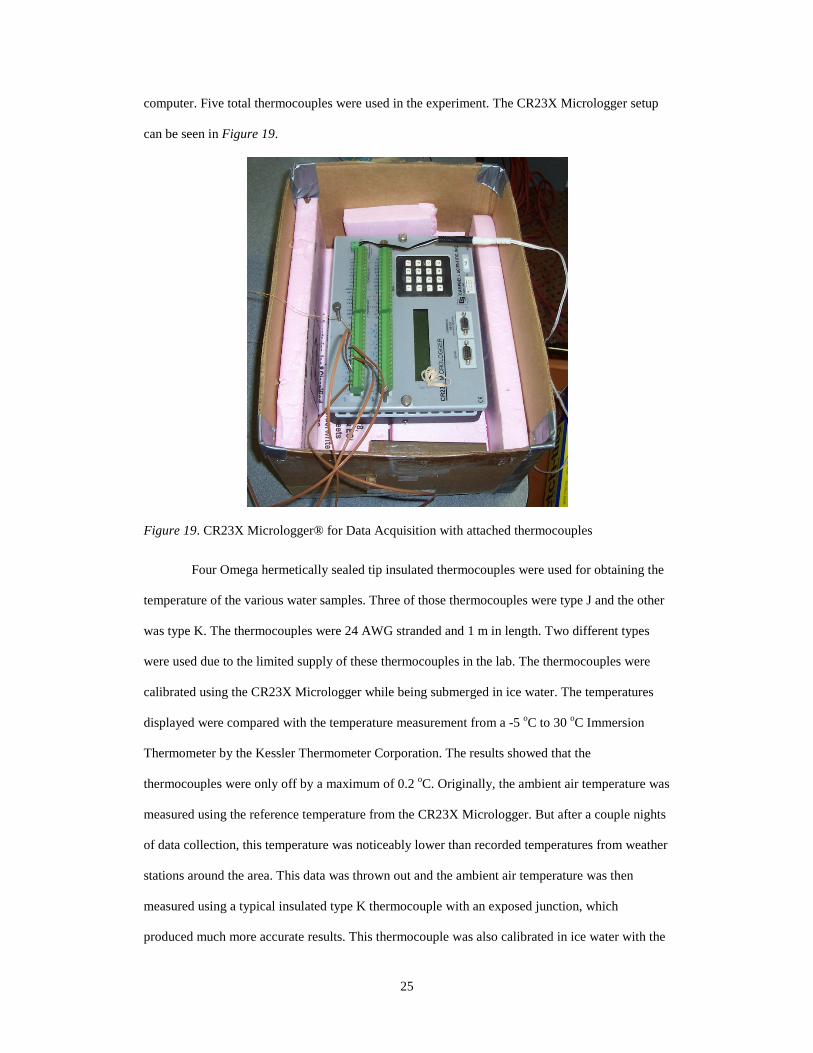
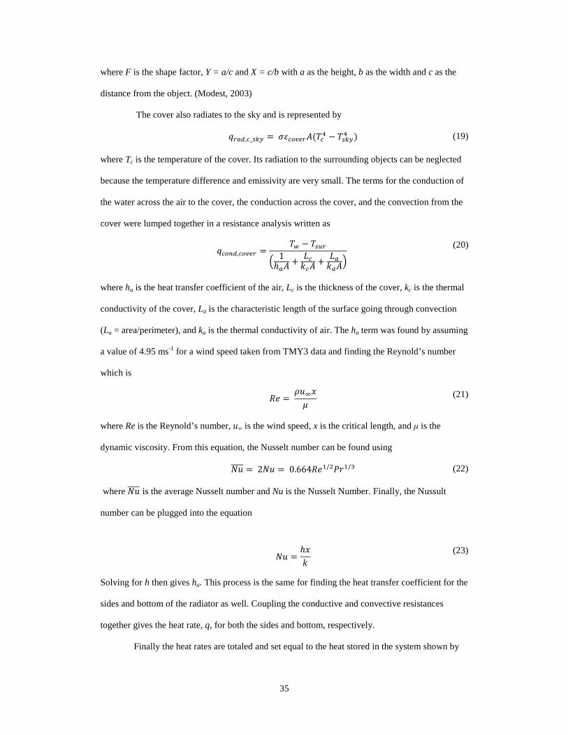
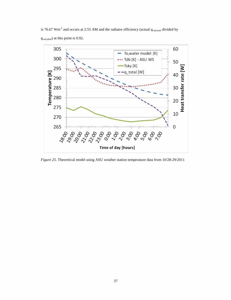