Study of Cell Nucleation in NanoPolymer Foams: An SCFT Approach

by

Yeongyoon Kim

A thesispresented to the University of Waterloo

in fulfillment of thethesis requirement for the degree of

Doctor of Philosophyin

Physics

Waterloo, Ontario, Canada, 2012

c© Yeongyoon Kim 2012

I hereby declare that I am the sole author of this thesis. This is a true copy of the thesis,including any required final revisions, as accepted by my examiners.

I understand that my thesis may be made electronically available to the public.

ii

Abstract

This thesis is about “nano-cellular” polymer foams, i.e., to understand nano-bubblenucleation and growth mechanisms, we used Self-Consistent Field Theory(SCFT) for theresearch.

Classical Nucleation Theory (CNT) is often used to calculate nucleation rates, butCNT has assumptions which break down for a nano-sized bubble: it assumes planar sharpinterfaces and bulk phases inside bubbles. Therefore, since the size of a nano-sized bubbleis comparable to the size of the polymer molecule, we assumed that a bubble surface is acurved surface, and we ivestigated effects of curvature on the nucleation barrier. SCFTresults show that sharper curvatures of smaller s cause a higher polymer configurationalentropy and lower internal energy, and also the collapse of the bulk phase for smaller bub-bles causes low internal energy. Consequently, the homogenous bubble nucleation barrierfor curved surfaces is much smaller than flat surface (CNT prediction).

We calculated direct predictions for maximum possible cell densities as a function ofbubble radius without calculation of nucleation barrier or nucleation rates in CNT. Ourresults show higher cell densities at higher solvent densities and lower temperatures. More-over, our cell density prediction reveals that rather than surface tension, the volume freeenergy, often labelled as a pressure difference in CNT, is the dominant factor for both celldensities and cell sizes. This is not predicted by CNT.

We also calculated direct predictions for the maximum possible cell densities as a func-tion of system volume in compressible systems. With an assumption that system pressurehas an optimal pressure which gives the maximal density of good quality foams (bulk phaseinside bubble), we calculated the inhomogeneous system pressure, the homogeneous sys-tem, and cell density as a function of system volume.Maximal cell prediction in compressible system shows the incompressible system predictionis the upperbound maximal cell density, and qualitatively consistent with the compressiblesystem results - higher cell densities at low temperatures and high solvent densities.In addition, our results show a bigger expansion as well as a high cell density at low tem-perature and high solvent density, but temperature is a more dominant factor than thesolvent density. From our results, we assume that a quick pressure dropping is required toget a better quality foam of a higher cell density.

iii

Acknowledgements

I would like to sincerely thank my supervisor, Prof. Russell B. Thompson. Withouthis help, this thesis wouldn’t have been completed. It has been a precious time for me tolearn from him and work with him for the past 4 years.

I would like to thank to my Graduate Committee members, Prof. Pu Chen, Prof.Bizheva Kostadinka, Prof. Bae-Yeun Ha, and Prof. Robert Wickham for their strong sup-port and kind guidance during my Ph. D. program. I would like to thank to my DefenceCommittee members, Prof. Apichart Linhananta, and Prof. Cecile Devaud for their kindand helpful comments on this thesis.

Especially, I would like to thank Prof. Chul B. Park for his help and encouragement.The conversations with him were very helpful for the researching this thesis.

I would like to thank to my colleagues in my office - Azadeh Bagheri, Kier von Konigslow,Yu-Cheng Su, Murthy SRC Ganti, Zheng Ma, Dr. Ying Jiang, Dr. Zi jian Long, Dr. SergeyMkrtchyan, and Dr. Wuyang Zhang, and my friends - Miok Park and Dr. Gopika Sree-nilayam. They were always willing to help me whenever I needed. It was a good time tohave been with them during my Ph. D. program.

And, especially I would like to thank to my current roommate, Ms. Becky Lawn, forher kind help with the grammar correction in this thesis.

Lastly, I would like to thank my beloved sisters and brother for their love. I dedicatethis thesis to my late parents, and I cannot help giving thanks to God since I believe inhis guidance in my life.

iv

Dedication

I dedicate this thesis to my parents.

v

Table of Contents

List of Figures viii

1 Introduction 1

1.1 Introduction to Polymer Foam . . . . . . . . . . . . . . . . . . . . . . . . . 2

1.2 Background literature . . . . . . . . . . . . . . . . . . . . . . . . . . . . . . 5

1.2.1 Theory . . . . . . . . . . . . . . . . . . . . . . . . . . . . . . . . . . 5

1.2.2 Experiment . . . . . . . . . . . . . . . . . . . . . . . . . . . . . . . 8

1.3 Outline of Thesis . . . . . . . . . . . . . . . . . . . . . . . . . . . . . . . . 11

2 Basic Theory 12

2.1 Classical Nucleation Theory . . . . . . . . . . . . . . . . . . . . . . . . . . 12

2.2 Self - Consistent Field Theory . . . . . . . . . . . . . . . . . . . . . . . . . 14

2.2.1 Modeling . . . . . . . . . . . . . . . . . . . . . . . . . . . . . . . . 14

2.2.2 Meanfield Theory and Density Functional Method . . . . . . . . . . 16

2.2.3 Numerical Method . . . . . . . . . . . . . . . . . . . . . . . . . . . 19

2.3 Theory for a Compressible System . . . . . . . . . . . . . . . . . . . . . . . 19

2.3.1 Compressible Lattice Liquid Theory . . . . . . . . . . . . . . . . . . 19

2.3.2 Equation of State . . . . . . . . . . . . . . . . . . . . . . . . . . . . 22

vi

3 Microscopic Origin of the Failure of Classical Nucleation Theory 24

3.1 Theory . . . . . . . . . . . . . . . . . . . . . . . . . . . . . . . . . . . . . . 25

3.2 Surface Tension, Volume Free Energy Density and Nucleation Barrier in aCurved Surface and a Flat Suface . . . . . . . . . . . . . . . . . . . . . . . 29

3.3 Microscopic Origins of the Failure of CNT . . . . . . . . . . . . . . . . . . 35

3.4 Discussion and Conclusion . . . . . . . . . . . . . . . . . . . . . . . . . . . 41

4 Maximal Cell Density and Temperature Effect on Cell Density 43

4.1 Calculation of Bubble Number Density . . . . . . . . . . . . . . . . . . . . 44

4.2 The ”Best” Foam . . . . . . . . . . . . . . . . . . . . . . . . . . . . . . . . 45

4.3 Temperature Effect on the Bubble Number Density . . . . . . . . . . . . . 52

4.4 Discussion and Conclusion . . . . . . . . . . . . . . . . . . . . . . . . . . . 58

5 Maximal Cell Density in Compressible Systems 59

5.1 Theory . . . . . . . . . . . . . . . . . . . . . . . . . . . . . . . . . . . . . . 60

5.1.1 Optimal Pressure . . . . . . . . . . . . . . . . . . . . . . . . . . . . 60

5.2 Maximal Cell Density . . . . . . . . . . . . . . . . . . . . . . . . . . . . . . 66

5.2.1 Different Temperature Cases with the Same Initial High Pressure . 66

5.2.2 Different Solvent Density Cases at the Same Temperature . . . . . 75

5.2.3 Different Temperature Cases with the Same Solvent Volume Fraction 75

5.3 Discussion and Conclusion . . . . . . . . . . . . . . . . . . . . . . . . . . . 78

6 Conclusions 82

Permissions 87

References 88

vii

List of Figures

1.1 Thermoplastic foaming process. . . . . . . . . . . . . . . . . . . . . . . . . 3

1.2 Schematic phase diagram of polymer solution at constant temperature usingpressure p and solvent molar fraction x as variables. In this diagram, thepressure quench ends in the unstable region,i.e., spinodal region. However,if the pressure quench ends in metastable region, then phase separation willstart by homogeneous nucleation. . . . . . . . . . . . . . . . . . . . . . . . 4

1.3 (a) Phase diagram at temperature kBT/ε = 0.75 ≈ 410C as a function ofpressure p and molar fraction x. Three constant nucleation barrier line areshown. We can see pressure jump would induce bubble nucleation. From[39] (b) Nucleation behavior of a hexadecane + carbon dioxide mixture atT = 400C. Full circles indicates the starting and ending point at which thehomogeneous nucleation is induced by pressure jump. Open circles markpoints at which no nucleation occur. From [50] . . . . . . . . . . . . . . . 7

1.4 (a) Processing temperature effect on foam structure. We can see small sizebubbles (high cell density) at low temperature. From [47] (b) Effects of(a)pressure drop rate (-dP/dt), (b) solvent density, (c) temperature. From[29] . . . . . . . . . . . . . . . . . . . . . . . . . . . . . . . . . . . . . . . 10

2.1 Plot of the nucleation barrier ∆F ∗ and critical radius R∗ . . . . . . . . . . 13

2.2 numerical method of solving self -consistent eqs. in real space . . . . . . . 20

viii

3.1 (a) Profile of the initial homogeneous system which has initial global vol-ume fraction values. (b) Profile of the bulk phase separated homogenoussystem which would be formed if there was no interface. Each bulk systemhas volume fraction values on either side of interface of the inhomogeneoussystem. Each bulk system volume V1 and V2 are determined by conservationof molecules. (c) Profile of the final inhomogeneous system after formationof a bubble, i.e., after formation of interface . . . . . . . . . . . . . . . . . 27

3.2 Homogeneous free energy versus global solvent volume fraction at χN = 140 30

3.3 (a) Profiles of local volume fractions of three different sizes of bubble in theflat surface case. (b) In this blow up graph, we can see that at the outsideof a bubble, three different sizes of bubble have the same solvent volumefraction value, which is the equilibrium value. . . . . . . . . . . . . . . . . 31

3.4 (a) Profiles of local volume fractions of three different sizes of bubble in thecurved surface case and one profile of a flat surface. (b) In this blow upgraph, we can see that in curved surface, three different sizes of bubble havedifferent solvent volume fraction values at the outside of a bubble. Comparedto the flat surface, in curved surface, smaller bubbles have more deviatedvolume fraction values from the equilibrium solvent volume fraction value. 32

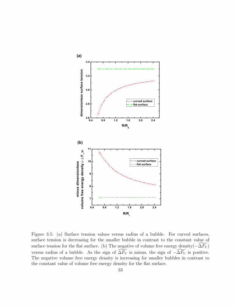
3.5 (a) Surface tension values versus radius of a bubble. For curved surfaces,surface tension is decreasing for the smaller bubble in contrast to the con-stant value of surface tension for the flat surface. (b) The negative of volume

free energy density(−∆̃FV ) versus radius of a bubble. As the sign of ∆̃FVis minus, the sign of −∆̃FV is positive. The negative volume free energydensity is increasing for smaller bubbles in contrast to the constant value ofvolume free energy density for the flat surface. . . . . . . . . . . . . . . . . 33

3.6 The solid line shows the free energy necessary to form a bubble of radius R(∆̃F (R)) in the flat surface case. The open circle and dotted line shows the

free energy necessary to form a bubble of radius R (∆̃F (R)) in the curvedsurface case. . . . . . . . . . . . . . . . . . . . . . . . . . . . . . . . . . . 34

3.7 Thermodynamic components of surface tension versus bubble radius R. In-creasing polymer configurational entropy is the main cause, and the de-creasing internal energy is a secondary cause of decreasing surface tensionfor smaller bubbles. Below 0.9 Rg, the internal energy shows a sharperdecreasing. . . . . . . . . . . . . . . . . . . . . . . . . . . . . . . . . . . . . 36

ix

3.8 In (a) and (b) the polymer has same configuration. However, for the flatsurface (a), since the surface is flat, the polymer has more contact withsolvent causing higher internal energy. (b) In the curved surface, since thesurface has curvature, the polymer has less contact with solvent causinglower internal energy. . . . . . . . . . . . . . . . . . . . . . . . . . . . . . 37

3.9 Thermodynamic components of volume free energy density versus bubbleradius R. By same mechanism of surface tension, together with increasinginternal energy, increasing entropy is the cause of increasing volume freeenergy density for smaller bubbles. . . . . . . . . . . . . . . . . . . . . . . 38

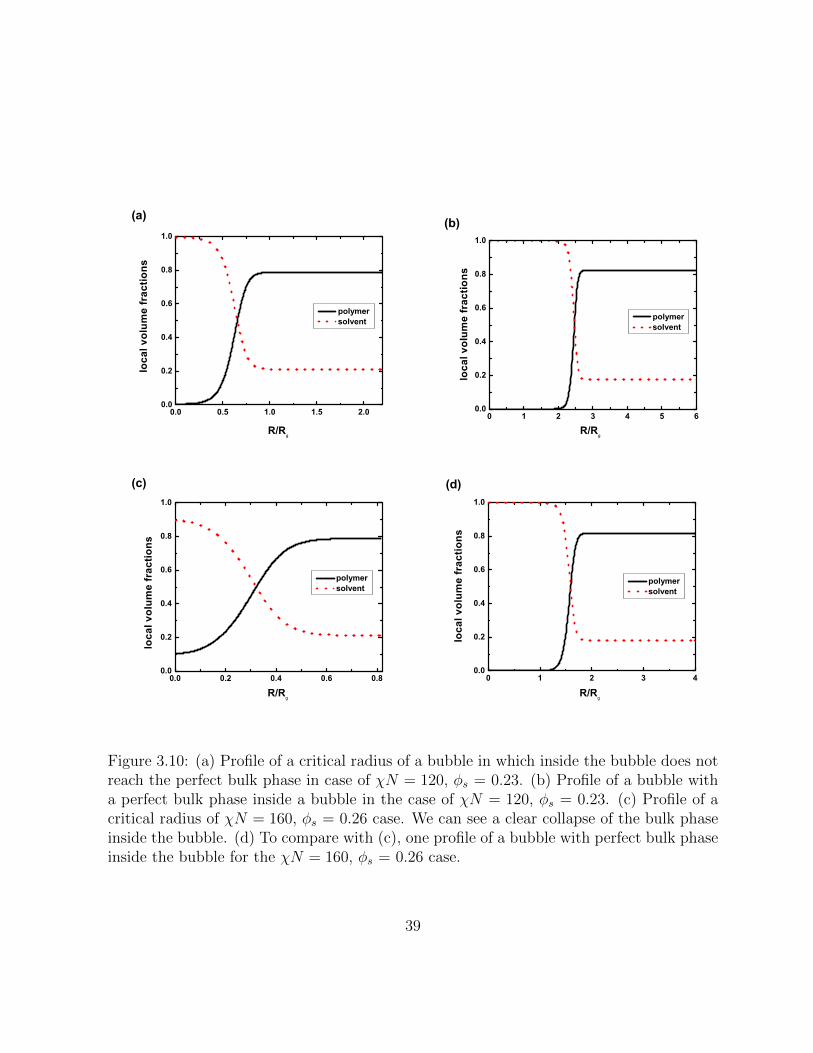
3.10 (a) Profile of a critical radius of a bubble in which inside the bubble does notreach the perfect bulk phase in case of χN = 120, φs = 0.23. (b) Profile ofa bubble with a perfect bulk phase inside a bubble in the case of χN = 120,φs = 0.23. (c) Profile of a critical radius of χN = 160, φs = 0.26 case. Wecan see a clear collapse of the bulk phase inside the bubble. (d) To comparewith (c), one profile of a bubble with perfect bulk phase inside the bubblefor the χN = 160, φs = 0.26 case. . . . . . . . . . . . . . . . . . . . . . . 39

3.11 Thermodynamic components of surface tension versus bubble radius R forthe case of χN = 160, φs = 0.26. Near the critical radius, at a small radiusof bubble, the decreasing internal energy becomes a main cause of decreasingsurface tension for smaller bubbles. . . . . . . . . . . . . . . . . . . . . . . 40

4.1 At χN = 160 (a) Dimensionless bubble number density versus radius of abubble. (b) Dimensionless bubble number density at the critical radius of abubble at different solvent volume fraction systems. . . . . . . . . . . . . . 46

4.2 At χN = 160 (a)Dimensionless bubble surface area per bubble box vol-ume (φs × Vbox) versus radius of bubble. (b) Dimensionless bubble numberdensity at the radius of the maximum of A/V . . . . . . . . . . . . . . . . . 47

4.3 At χN = 160 (a) Solvent volume fraction value at the center of bubbleversus radius of the bubble (b) Dimensionless bubble number density at thebubble radius R = 0.7Rg at different solvent volume fraction systems . . . 49

4.4 At χN = 160, dimensionless bubble number density at different solventvolume fraction systems in view of maximal number density, maximal bubblesurface area, and bulk condition at the center of a bubble. . . . . . . . . . 50

4.5 At χN = 160,(a) Dimensionless surface tension γ versus radius of bubble.(b) - ∆FV at R = 0.7Rg at different solvent volume fraction systems. . . . 51

x

4.6 Solvent volume fraction value at the center of a bubble versus radius of thebubble at different solvent volume fraction systems at χN= 160. (b) Surfacetension versus radius of a bubble at different solvent volume fraction systemsat χN = 120 and at χN = 160 . . . . . . . . . . . . . . . . . . . . . . . . 53

4.7 At χN = 120, (a) Negative volume free energy density ∆FV and (b) dimen-sionless bubble number density at different solvent volume fraction systems 54

4.8 At χN = 160, φs = 0.29 and χN = 120, φs = 0.29 (a) Dimensionless bubblenumber density. (b)∆FV versus radius of bubble . . . . . . . . . . . . . . . 56

4.9 At different solvent density systems at χN = 120 and χN = 160 (a) −∆FV(b) Dimensionless bubble number density . . . . . . . . . . . . . . . . . . . 57

5.1 (a) Plot of several bubble pressures at different system volumes. (b) Blowup of several bubble pressures at Vsys = 1.1V0. (c) Three representativebubble pressures at Vsys = 1.1V0. . . . . . . . . . . . . . . . . . . . . . . . 63

5.2 (a) Cell density versus bubble radius at different system volumes. (b)Abubble/Vbox versus bubble radius at different system volume. . . . . . . . . 64

5.3 (a) Solvent volume fraction value at the center of bubble versus bubbleradius at different system volumes. (b) Plot of three optimal pressuress ofsmallest cell, maximum Abubble/Vbox,and ϕs(0) ≈ 1 at the center of bubble. . 65

5.4 At T = 1.5 (a) Three optimal pressures versus system volume. (b) Blow upplot of optimal pressure values at Vsys = 1.1V0. . . . . . . . . . . . . . . . . 67

5.5 Three maximal cell densities corresponding to three optimal pressures versussystem volume at T = 1.5. . . . . . . . . . . . . . . . . . . . . . . . . . . . 68

5.6 At T = 2.0 (a) Three optimal pressures versus system volume. (b) Blow upplot of optimal pressure values at Vsys = 1.1V0. . . . . . . . . . . . . . . . 70

5.7 Three maximal cell densities corresponding to the three optimal pressuresversus system volume at T = 2.0. . . . . . . . . . . . . . . . . . . . . . . . 71

5.8 At T = 1.5 and T = 2.0 (a) Pressure of the inhomogeneous system and thehomogeneous system versus system volume (b) Blow up plot of the pressureat V = 1.05V0. (c) Blow up plot of the pressure at V = 1.3V0. . . . . . . . 73

5.9 Cell density versus system volume at T = 1.5 and T = 2.0 . . . . . . . . . 74

xi

5.10 At different solvent volume fractions (solubilities) for χN = 120 (a) Pressureof the inhomogeneous system and the homogeneous system versus systemvolume (b) Blow up plot of the pressure V = 1.05V0. (c) Blow up plot ofthe pressure at V = 1.1V0 . . . . . . . . . . . . . . . . . . . . . . . . . . . 76

5.11 Cell density versus system volume at different solvent volume fractions (sol-ubilities) for χN = 120 . . . . . . . . . . . . . . . . . . . . . . . . . . . . 77

5.12 At χN = 120, φs = 0.32 and χN = 160, φs = 0.32 (a) Pressure of theinhomogeneous system and the homogeneous system versus system volume(b) Blow up plot of pressure at V = 1.05V0. (c) Blow up plot of pressure atV = 1.1V0 . . . . . . . . . . . . . . . . . . . . . . . . . . . . . . . . . . . . 79

5.13 Cell density versus system volume at χN = 120, φs = 0.32 and χN = 160,φs = 0.32. . . . . . . . . . . . . . . . . . . . . . . . . . . . . . . . . . . . . 80

xii

Chapter 1

Introduction

Microcellular foam is a polymeric foam with a cell size less than 10 µm and a cell den-sity greater than 109 cells/cm3. It was first developed at the Massachusetts Institute ofTechnology [33] in the early 1980s to increase the toughness of materials and reduce thematerials consumption. Because of the small cell size, microcellular foams show increasedthermal and electrical insulation and superior mechanical properties. With these benefits,microcellular foams also reduce the material cost.Therefore, intensive efforts have been made to develop foams with a higher cell density andwith smaller bubble sizes such as nano-size. Nanocellular foam is a polymeric foam withcell size less than 0.1µm and cell density greater than 1015 cells/cm3. In recent years, sev-eral successful implementations of nanocellular foams have been reported [22, 11, 32, 69].However, due to the high cost and slow production rates, commercial application has beenlimited.Thus, for the large -scale production of a high quality foam such as a nanocellular poly-meric foam, it is required to understand the mechanism of bubble nucleation and growththat is influenced by foaming processing parameters such as temperature, pressure, solventconcentration, and depressurization rate, etc.

To have foams of a high cell density with small-sized bubbles, a high nucleation rateis required. People often use classical nucleation theory (CNT) for simplicity of approach.However, CNT has been shown to be insufficient in many cases [53, 42, 38, 44] , espe-cially for small-size bubble nucleation. Since we investigate nanocellular foams, we usedself-consitent field theory (SCFT), which is a mean field equilibrium statistical mechani-cal theory containing a microscopic model of polymer degrees of freedom. In addition, asthe cell size is comparable to the polymer molecular size, we assumed bubble surface as a

1

curved surface in contrast to the flat surface assumption for a bubble surface in CNT. Forsimplicity, we used an incompressible polymer + solvent system. We observed that the ho-mogeneous nucleation barrier of the curved surface is much smaller than the correspondingvalue of the flat surface. We investigated the microscopic origin of this by studying thethermodynamic components of the free energy.

To calculate the bubble number density by using CNT, one needs to calculate an ex-ponential prefactor and integrate over time of the nucleation rate. By using our model, wedirectly calculated the maximal cell density without the calculation in CNT.Based on our results, we investigated the cell density dependence on temperature and sol-vent density. Our results were qualitatively consistent with experimental results, but therewas qualitative difference between the expectation of SCFT and CNT. It turns out thatsurface tension is not a dominant factor for cell density and size.

To investigate a more realistic system,i.e., a compressible system, we used a hole-basedSCFT developed by Hong and Noolandi[17]. With an assumption that a system has anoptimal pressure which gives the best form,i.e., a foam which have the smallest bubblesthat reached the bulk phase at the center, we calculated system pressure, the maximal celldensity, expansion ratio, and void fraction as a function of system volume. Based on ourresult, we investigated cell density, expansion ratio, cell morphology for different processingconditions such as different temperatures and solvent densities.

In the first section, we briefly introduce polymer foam. In section 2, we present back-ground literature of theory and experiment, and in section 3, we outline the thesis.

1.1 Introduction to Polymer Foam

The word ”foam” originates from the medieval German word veim which means ”froth”[63]; however, the terminology ”foam” refers to bubbles dispersed in a dense continuum likea solid. Polymer foams, which consist of polymer matrices with fluid bubble inclusions, areused in furniture, automotive parts, construction materials, insulation board, and manyother areas [26].

Foaming is a temperature or pressure controlled phenomenon. Gas foaming can begenerated by dropping pressure or temperature. In this thesis we only investigate pres-

2

pressure

vo

lum

e

temperature

gas

polymer

gas

polymer

air

Figure 1.1: Thermoplastic foaming process.

sure induced foaming. Fig.(1.1) explains the process of thermoplastic foaming induced bypressure dropping. First, from state (A) to (B) by raising temperature and pressure, theraw plastic materials is heated and pressurized and blowing agent (solvent) is dissolved atthis fluid-like melt to form a homogeneous melt solution. Then, from state (B) to (C),suddenly by dropping pressure, the foaming processing occurs due to the instant supersat-uration induced by the pressure drop. And, finally from state (C) to (D) by replacing thegas to air the final foam product is made.

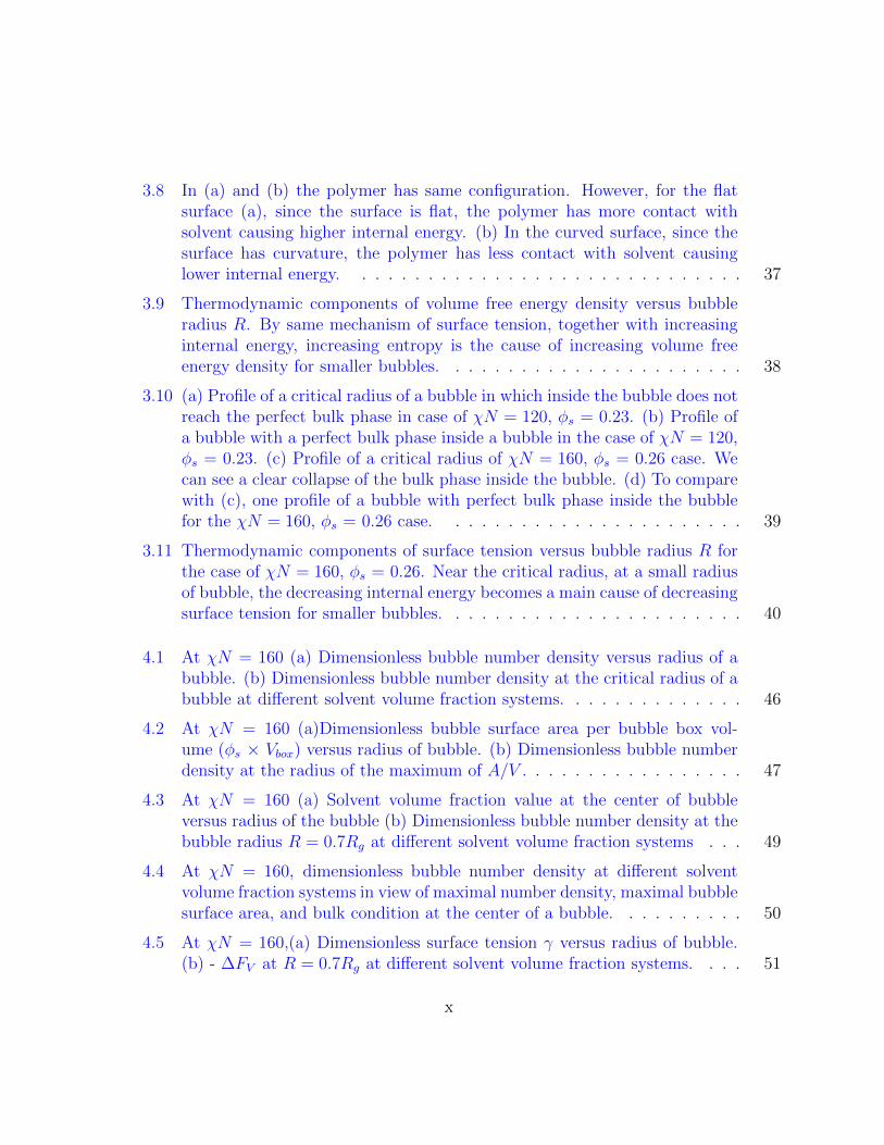
We regard foaming as a phenomenon of a phase transition from one phase to two phases.Fig.(1.2) shows a schematic phase diagram of a compressible polymer solution at constanttemperature. In this diagram, variables are pressure p and solvent molar fraction x. Wecan see the phase separation between the polymer and the molecular solvent is induced bya pressure jump, and Fig.(1.2) shows that the system would be separated two phases, i.e.,polymer with some dissolved solvent molecules and solvent (molar fraction x = 1) in thevapor phase. In the diagram, it is assumed the pressure jump ends in unstable (spinodal)region. However, if the pressure quench ends in the metastable (nucleation and growth)region, the phase separation will occur by homogeneous nucleation.

3

Figure 1.2: Schematic phase diagram of polymer solution at constant temperature usingpressure p and solvent molar fraction x as variables. In this diagram, the pressure quenchends in the unstable region,i.e., spinodal region. However, if the pressure quench ends inmetastable region, then phase separation will start by homogeneous nucleation.

On the other hand, there are fundamental relationships between foam structure andits properties. The properties of polymeric foams are determined by the following struc-tural parameters: cell density, cell size and its distribution, expansion ratio, and open cellcontent,etc. The density and distribution of cells are critical parameters in determiningthe final property of the polymeric foam. Also, the cell size is an important factor. It iswell known that insulation ability depends on the cell size. According to studies of mi-crocellular foam with a cell size on the order of 10 microns, small cells provide a betterenergy absorption capability. In addition, plastics with a high cell density and uniformcell density show superior mechanical properties such as higher toughness as well as betterthermal and acoustic insulation properties. [2, 45].And, the cells are divided into the open cell and closed cell. Open-cells are connected witheach other, and closed-cells are discrete, each surrounded by the polymer. Open-cell andclosed-cell each has advantages and disadvantages - open cell is desirable in gas exchange,absorption and sound deadening, but has poor mechanical properties. Thus, open cell con-tent is not desirable for closed-cell foams. In addition, the blowing agent(solvent)’s quality,quantity and nature are also important factors for the production of a foamed structure

4

with certain desired properties.

Therefore, there are enormous efforts to get an insight of mechanisms of bubble nucle-ation and growth and proper foaming process conditions for a desired foam morphology.In particular, the improvements of quality of foam are sought by reducing the cell size tonanometer dimensions for nanocellular foams.

1.2 Background literature

1.2.1 Theory

Colton and Suh [5, 6] used CNT as the basis to develop a model of the nucleation of mi-crocellular foam with additives. They used a polystyrene-zinc stearete system and usednitrogen and carbon dioxide as additives. They reported that the theoretical and experi-mental results reasonably agree. However, they considered that homogeneous nucleationand heterogeneous nucleation occur together, and that heterogeneous nucleation dominatesbecause of a high homogeneous nucleation barrier. It is considered that their classical ho-mogeneous nucleation is able to fully describe the nucleation activity.

Goel and Beckman [13] generated microcellular foam by a pressure quench in a CO2 -swollen poly(methymethacrylate), PMMA, sample. They used CNT for their model, andfound that agreement between experimental data and model calculation is very good athigh pressure. But, they observed a limited nucleation at low pressure (∼10MPa), andthey explained that it could be due to a high heterogeneous nucleation at low pressure. Inaddition, in their model, for the surface tension, they used the correlation for the surfacetension mixture given by Reid[?].

Shukla and Koelling [53] used a modified CNT which accounts for diffusional and vis-cosity constraints to calculate the rate of homogeneous nucleation of microcellular foamof a polystyrene - CO2 system. They found that the capillary approximation of CNT isnot valid for bubble nucleation. After a correction accounting for the curvature effect ofsurface tension along the lines suggested by Tolman [59], they observed the theoreticallypredicted rate is consistent with the experimental results.

5

On the other hand, there are also Monte Carlo simulation studies of droplet nucleationby using CNT. Neimark and Vishynyakov [42] studied nucleation barriers for droplets inLennard-Jones fluids. Based on their data by MC simulation, they investigated the limitsof applicability of the capillarity approximation of CNT and the Tolman equation. Theyreport that the Tolman equation can not be approximated for small droplets of a radiusless than four molecular diameters.

Merikanto and Vehkamaki [38] used CNT based on a liquid drop model. They showedthat CNT can be used to fit small cluster sizes, but there was error in modeling the smallestof clusters. They show that the liquid model can be used to calculate the work related toaddition of monomer to cluster sizes between 8 to 50 molecules. But they pointed out thatthe microscopic effect related to the formation of the smallest clusters, the total clusterwork given by CNT might introduce a large correction term.

Beyond CNT, Lee and Flumerfelt [24] used the integral overall energy balance and theintegral Clausius - Duhem inequality to analyze a bubble nucleation experiment. Theyobserved that for molten low-density polyethylene with dissolved nitrogen, surface tensiondecreases as the cluster size becomes smaller, and they explained the reduction of surfacetension is due to the dissolved gas in molten polymer and small critical cluster size.

As a nonclassical theory for a homogeneous nucleation of gas to liquid, Oxtoby andEvans [44] used a density functional method. They used a grand potential to be a func-tional of the inhomogeneous density, and used the Yukawa potential. Thus, the gas-liquidsurface free energy for a planar interface is inversely proportional to λ. λ is a parameterof Yukawa potential which is related to a range of attractive potential. Oxtoby and Evansobserved that the agreement of the nonclassical and classical expectation depends stronglyon the λ. For λ = 1,i.e., the range of attractive potential is equal to the hard spherediameter, the deviation between nonclassical and classical results for the bubble formationfrom liquid is much bigger than the liquid formation from gas. Especially, the classicaltheory predicts no transition to occur because the potential barrier is too high. Theyalso observed that in the density functional calculation, the potential barrier vanished atthe spinodal in contrast to the potential barrier which has a finite value at spinodal in CNT.

Ghosh and Ghosh[12] presented a theory for homogeneous nucleation using DFT witha square gradient approximation for the free energy functional to get an analytical ex-pression for the size-dependent free energy formation of a liquid drop. They applied the

6

Figure 1.3: (a) Phase diagram at temperature kBT/ε = 0.75 ≈ 410C as a function ofpressure p and molar fraction x. Three constant nucleation barrier line are shown. Wecan see pressure jump would induce bubble nucleation. From [39] (b) Nucleation behaviorof a hexadecane + carbon dioxide mixture at T = 400C. Full circles indicates the startingand ending point at which the homogeneous nucleation is induced by pressure jump. Opencircles mark points at which no nucleation occur. From [50]

theory for droplet nucleation from supersaturated vapor of Lennard-Jones fluid, and foundthe nucleation barrier calculated by the nonclassical theory is significantly lower than theprediction of CNT.

Parra and Grana [49] analyzed the influence of attractive pair-potentials in densityfunctional models of homogeneous nucleation. They showed that if asymptotic decay atinfinity of attractive potential is strong enough, then the ratio of nucleation barrier of thedensity functional and corresponding classical result weakly dependent on the form of thepair-potential. However, if the asymptotic decay at infinity is not weak enough, then thenucleation barrier ratio decreases significantly with interaction potential strength.

Binder et. al.[4] used SCFT as a nonclassical theory for homogeneous bubble nucleationin polymer + solvent systems. They chose the mixture of hexadecane with carbon dioxideas a polymer + solvent system. In the SCF calculation, they used the grand canonicalensemble and observed only critical bubbles. As we can see Fig. 1.4, they could reproducequalitative features of experimental data from Rathke et al.[50], i.e., measured nucleation

7

rate in hexadecane + CO2 mixture at 400C. They observed that in Fig. 1.4(a), as themolar fraction increases at constant pressure the nucleation barrier decreases, and it van-ishes at the spinodal, which is similar what we observe in our research - as pressure dropsat constant temperature the nucleation barrier approaches to the zero, i.e., approaches tospinodal.

We used SCFT in this thesis. It is a mean field equilibrium statistical equilibrium the-ory, but Oxtoby[43] pointed out that in the grand canonical ensemble in which the numberof molecules fluctuate, a dynamically unstable state like a critical radius is not stable, butin the canonical ensemble in which the number of molecules is fixed, a system consistingof a critical radius surrounded by original phase is thermodynamically stable.

In microcellular foams Goel and Beckman [13] reported that their results of microcellu-lar foam can be fit with CNT for high pressure, but they observed a limited nucleation atlow pressure and explained that it is due to a high heterogeneous nucleation at low pres-sure. For a homogeneous nucleation, Shukla and Kellings [53] were only able to fit withCNT when they modified their surface tension using the Tolman approximation. However,MC studies [42][38] showed that even the Tolman equation cannot be approximated forsmall droplets of a radius less than four molecular diameters, and pointed that microscopiceffects related to the smallest cluster might introduce a large correction term to CNT ex-pectations. Lee and Flumerfelt [24] showed that surface tension decreases as the clustersize becomes smaller, and the surface tension reduction is the cause of the seriously under-predicted nucleation rate of CNT. However, they couldn’t explain the microscopic originof the surface reduction at smaller cluster sizes. They assumed a perfectly sharp bubbleinterface and didn’t use a model containing polymer degrees of freedom. In this thesis, weused SCFT which is a coarse-grained microscopic model, and investigated the microscopicorigin of the failure of CNT.

1.2.2 Experiment

To make a desired foam morphology there have been enormous efforts to choose correctcombination of processing conditions such as temperature, solvent concentration, pressuredropping rate, etc.

Goel and Beckman [13], Leung et. al. [29], Ito et. al. [19], Tsivintzelis et. al. [60], Han

8

et. al. [14] investigated cell density dependence on solvent density by using a polymer withCO2. Their results show higher cell density with increased solvent density. Thus, therehave been also intensive researches for the solubility. [31, 15, 52, 30]

Also, Goel and Beckman [13], Leung et. al. [29],Tsivintzelis et. al.[60], Matuana et.al.[37], Wong et. al.[65] also investigated cell density dependence on temperature by usinga polymer with CO2. Higher cell density with lower temperature is observed

Surface tension is known to be a crucial factor in polymer foaming processes. Thus,there is much research about the surface tension. [48, 57, 57, 64, 9, 8, 27] Park et al.[48] investigated effect of temperature and pressure in surface tension of polystyrene insupercritical CO2. Their results show that surface tension decreases for high temperatureand pressure.However, we notice that Goel and Beckman[13] needed a low surface tension at low temper-ature to fit to CNT and their increased cell density at low temperature. Experimentally,Leung et. al.[28] observed high cell density at low temperature and found the surfacetension has a minimal effect. Amon and Deson [1] also found surface tension to be unim-portant to the foaming process in their theoretical work. We observed that the drivingforce to make the bubble,i.e., pressure difference in CNT, is a more dominant factor thanthe surface tension.

Aside from cell density and cell size, foam properties are also determined by foamvolume expansion ratio or open-cell content. There are efforts to know the expansionbehavior. [40, 66, 47, 41] The experimental results showed the volume expansion ratioincreased with decreased temperature. Fig. 1.3(a) shows Park et. al.’s result [47]. As forthe processing condition, except temperature or solvent density mentioned above, thereare also works to see effects of pressure dropping rate on foam properties. [45, 29, 25].Leung and Guo [29] investigated cell density by using polycarbonate foams blown withsupercritical CO2. Their results show high cell densities at higher pressure dropping rate.Fig. 1.3(b) shows their result.

We compared qualitatively our theoretical results,i.e., foam morphology dependence onprocessing conditions, with these experimental results.

9

(a)

T c = 170°C

T c = 150°C

T c = 120°C

(b)

(c)

(a) (b)

Figure 1.4: (a) Processing temperature effect on foam structure. We can see small sizebubbles (high cell density) at low temperature. From [47] (b) Effects of (a)pressure droprate (-dP/dt), (b) solvent density, (c) temperature. From [29]

10

1.3 Outline of Thesis

In chapter 2, we introduce basic theories used in this thesis.

In chapter 3, for nano-sized bubbles, since the curvature of the bubble surface is compa-rable to the size of the polymer molecule, we represent bubble surface as a curved surface.We investigate the effect of curvature on the nucleation energy of a bubble, and our re-sults show that a nano-sized polymeric bubble has a much smaller nucleation energy thanCNT predicts. We also investigate the microscopic origins of the failure of CNT for nano-polymeric foams.

In chapter 4, by using SCFT and our model, we calculate direct predictions for themaximal possible cell densities as a function of radius of a bubble without calculatingthe nucleation energy and nucleation rate, as is required for CNT. With the results ofcell density at different temperatures and solvent densities, we investigate the effects oftemperature and solvent density on cell density. We present result which contradict CNTprediction, and it is found that for different temperatures, the volume free energy densityis a more dominant factor than surface tension for both cell density and cell size.

In chapter 5, we drop the incompressible limitation used in chapter 3 and chapter 4.By using a hole-based SCFT developed by Hong and Noolandi, we calculate system pres-sure as a function of system volume. For the calculations, we assume our system has anoptimal pressure of the best foam in which the bulk phase is reached inside the bubble.Then, we calculate the maximal cell density and polymer density outside a bubble as wellas system pressure as a function of system volume. We investigate qualitatively the systemexpansion ratio and open cell content for different processing conditions such as differenttemperatures, solvent densities, and the pressure drop rate.

In chapter 6, conclusions and discussion are presented.

11

Chapter 2

Basic Theory

2.1 Classical Nucleation Theory

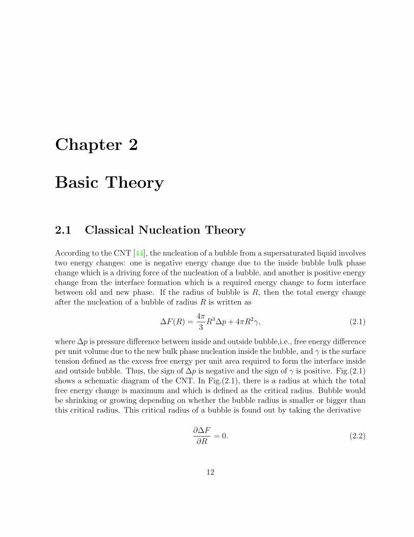
According to the CNT [44], the nucleation of a bubble from a supersaturated liquid involvestwo energy changes: one is negative energy change due to the inside bubble bulk phasechange which is a driving force of the nucleation of a bubble, and another is positive energychange from the interface formation which is a required energy change to form interfacebetween old and new phase. If the radius of bubble is R, then the total energy changeafter the nucleation of a bubble of radius R is written as

∆F (R) =4π

3R3∆p+ 4πR2γ, (2.1)

where ∆p is pressure difference between inside and outside bubble,i.e., free energy differenceper unit volume due to the new bulk phase nucleation inside the bubble, and γ is the surfacetension defined as the excess free energy per unit area required to form the interface insideand outside bubble. Thus, the sign of ∆p is negative and the sign of γ is positive. Fig.(2.1)shows a schematic diagram of the CNT. In Fig.(2.1), there is a radius at which the totalfree energy change is maximum and which is defined as the critical radius. Bubble wouldbe shrinking or growing depending on whether the bubble radius is smaller or bigger thanthis critical radius. This critical radius of a bubble is found out by taking the derivative

∂∆F

∂R= 0. (2.2)

12

0

F

radius

bulk energy interfacial energy total energy

F*

R*

Figure 2.1: Plot of the nucleation barrier ∆F ∗ and critical radius R∗

The critical radius is then found to be

R∗ = − 2γ

∆p(2.3)

Then, the nucleation barrier is defined as the total free energy at the critical radius,i.e., the bubble should overcome this nucleation barrier to grow. The nucleation barrier issimply found by substituting the critical radius in eq.(2.1)

∆F ∗ =16π

3

(γ3

∆p2

). (2.4)

13

According to CNT, the steady-state nucleation rate has the form

J = J0 exp

(−∆F ∗

kT

), (2.5)

where J0 is a dynamical prefactor that is related to the characteristic time scale for motionin the system, k is Bolzmann constant, and T is absolute temperature. Here we can seethat the nucleation barrier is a very important factor in determining the nucleation rate.If nucleation barrier is small, then the nucleation rate is increased exponentially. However,in CNT there are several limitations to calculate the nucleation barrier of nano-polymerbubble.

First of all, CNT assumes both the inside and outside bubble phases are bulk phase nomatter how much small the bubble size is. If the bubble size is nano-size, then the bubblemight be all interface without a bulk phase in the interior of the bubble, i.e., bubble mightnever reach the bulk phase at the center of a bubble. Secondly, CNT assumes the surfaceis a sharp flat surface, but for small bubbles like nano-sized bubbles, the surface curvatureis significant, so it is not proper to assume there is no curvature. The curvature effecton surface tension might be very significant. Thirdly, in CNT, they assume there is nothickness in interface assuming the interface be like step function. Due to these above CNTassumptions that are not suitable for nano-sized bubbles, CNT nucleation rate predictionsmight deviate significantly from real nucleation rates in nano-sized bubbles.

2.2 Self - Consistent Field Theory

We use Self - Consistent Field Theory(SCFT) to calculate the total free energy changebefore and after formation of a bubble. SCFT[35, 10] is an equilibrium statistical mechan-ical mean field theory. Oxtoby[43] pointed out that bubbles are stable as opposed to thegrand canonical ensemble in canonical ensemble formalism where the free energies can becorrectly calculated. Thus, SCFT is suitable to calculate free energy of inhomogeneouspolymer system. We use constraint free, canonical ensemble in this thesis. The bubbleswe study are stable against growth above the critical radius.

2.2.1 Modeling

Our system is a homopolymer + solvent system. We use a standard coarse-grained Gaus-sian string model for the polymer, so the polymer is described as a chain of segments whose

14

orientation is random and the distribution of a segment length is Gaussian distribution[34].We model the solvent as a particle which has an excluded volume. For the interaction ofmolecules, we assume there are contact interactions between polymer segments, solventmolecules,and polymer segment and solvent molecule. Then, the Hamiltonian of our sys-tem is written as the polymer configuration energy which is like a segment stretching energyto treat polymer configurational entropy plus the interaction energy between molecules.Hamiltonian H is given by

H =

np∑i=1

3

2Na2

∫ 1

0

ds

∣∣∣∣drα(s)

ds

∣∣∣∣2 + χ

∫φ̂p(r)φ̂s(r)dr, (2.6)

where a is a statistical segment length, rα(s) is a space curve of a polymer, χ is theFlory-Huggins parameter which is a segregation parameter defined by

χ = χ̃ps −1

2(χ̃pp + χ̃ss)

χ̃ij =ρiρjkBT

∫Vij(|r|)dr. (2.7)

φ̂p(r),φ̂s(r) are the concentration operator of polymer and solvent molecule at a given pointr and are defined as

φ̂p(r) =N

ρp

np∑α=1

∫ 1

0

dsδ (r− rα(s)) (2.8)

φ̂s(r) =1

ρs

ns∑i=1

δ (r− ri) , (2.9)

where N is the degree of polymerization based on the polymer segment volume ρ−1p , andnp, ns are number of polymer molecules and solvent molecules respectively, and ρ−1p , ρ−1sare the volumes of one segment of polymer molecule and a solvent molecule, respectively.Then, with an incompressible system constraint, the partition function of our system iswritten

Z =1

np!ns!

∫ np∏α=1

D̃rα

∫ ns∏i=1

driδ(

1− φ̂p(r)− φ̂s(r))

× exp

(−χρp

∫φ̂p(r)φ̂s(r)dr

), (2.10)

where

D̃rα ≡ Drα exp

(−3

2Na2

∫ 1

0

da

∣∣∣∣drα(s)

ds

∣∣∣∣2)

(2.11)

15

, which is a functional integral of all possible configurations of a polymer.

2.2.2 Meanfield Theory and Density Functional Method

To transform the operators φ̂p and φ̂s to the field functions Φp and Φs one uses the δfunctional integral representation,∫

DΦpδ[Φp(r)− φ̂p(r)]F (Φp(r)) = F (φ̂p(r)) (2.12)∫DΦsδ[Φs(r)− φ̂s(r)]F (Φs(r)) = F (φ̂s(r)) (2.13)

δ[Φp(r)− φ̂p(r)] =

∫ +i∞

−i∞DWp exp

[ρpN

∫drWp(r)(Φp(r)− φ̂p(r))

](2.14)

δ[Φsr)− φ̂s(r)] =

∫ +i∞

−i∞DWs exp

[ρs

∫drWs(r)(Φs(r)− φ̂s(r))

](2.15)

By using above expressions, partition function Z is written

Z =1

np!ns!

∫ np∏α=1

D̃rα

∫ ns∏i=1

dri

∫DΦpDΦsDWpDWsDΞ

× exp

[ρpN

∫drWp(r)(Φp(r)− φ̂p(r)) + ρs

∫drWs(r)(Φs(r)− φ̂s(r))

+ρpN

∫dr (Ξ(r)(1− Φp(r)− Φs(r))− χNΦp(r)Φs(r))

](2.16)

Here, by using the definition of φ̂p(r) and φ̂s(r),

ρpN

∫drWp(r)φ̂p(r)− ρs

∫drWs(r)φ̂s(r) = −

np∑α=1

∫dsWp(rα(s))−

ns∑i=1

Ws(ri) (2.17)

Now, the partition function is written with field functions

Z =1

np!ns!

∫DΦpDΦsDWpDWsDΞQnp

p Qnss

× exp

[ρpN

∫dr(Wp(r)Φp(r) +Ws(r)Φs(r)

+Ξ(r)(1− Φp(r)− Φs(r))− χNΦp(r)Φs(r))], (2.18)

16

where

Qp ≡∫D̃rαe

−∫ 10 dsWp(rα(s)) (2.19)

Qs ≡∫dre−αWs(r) (2.20)

which are the partition functions of a polymer and solvent molecule respectively basedon subject to the fields ωp and ωs. α is the ratio of the volume of a solvent molecule topolymer molecule (α = ρp/(Nρs)). Finally, we obtain the partition function

Z =1

np!ns!

∫DΦpDΦsDWpDWsDΞ exp

(− F

kBT

), (2.21)

where

F

kBT= np lnQp − ns lnQs

−ρpN

∫dr[Ξ(r)(1− Φp(~r)− Φs(r))− χNΦp(r)Φs(r)

+Wp(r)Φp(r) +Ws(r)Φs(r)]. (2.22)

Now, though we got the partition function expression of our system, we can not calculatethe functional integrals. Thus, in SCFT one approximates this integral by the extremumof the integrand. By the Saddle -Point method[7], we take the minimum Helmholtz freeenergy F = −kBT lnZ as our inhomogeneous system free energy. Thus, our inhomogeneousfree energy is given by F [ϕp, ϕs, ωp, ωs, ξ], where ϕp, ϕs, ωp, ωs, ξ are the functions for whichF has the minimum. From the minimum condition - the functional derivative of eachvariable is zero - we get following self consistent equations.

ωp(r) = χNϕs(r) + ξ(r) (2.23)

ωs(r) = χNϕp(r) + ξ(r) (2.24)

ϕp(r) + ϕs(r) = 1 (2.25)

ϕp(r) = −φpVQp

δQp

δωp(r)(2.26)

ϕs(r) =φsV

Qs

e−αωs(r) (2.27)

17

By solving these equations self-consistently, the inhomogeneous free energy is obtained.At this point, we can use an alternative expression of the partition function of a polymermolecule, i.e.,

Qp =

∫drq(r, 1), (2.28)

where the end-segment distribution function q(~r, 1) is given by

q(r, 1) =

∫DrαP [rα; 0, 1]δ(r− rα(1)) exp[−

∫ 1

0

ωp(rα(s))ds] (2.29)

which is the functional integral over all configuration with the functionals

P [rα; 0, 1] ∝ exp

{− 3

2Na2

∫ 1

0

ds| dds

rα(s)|2}

(2.30)

Then,with the identity [16],(3

2πNa2∆s

) 32

exp

[− 3

2Na2∆s|r− s|2

]= exp

(−1

6Na2∆s∇2

r

)δ(r− s), (2.31)

this end-segment distribution function satisfies the modified diffusion equation.

∂q(r, s)

∂s=

1

6Na2∇2q(r, s)− ωp(r)q(r, s) (2.32)

By solving this modified diffusion equation,the ϕp(r) is given by

ϕp(r) =φpV

Qp

∫ 1

0

q(r, s)ds (2.33)

From those self-consistent equations, once we obtain ϕp(r), ϕs(r), ωp(r), ωs(r), ξ(r), thedimensionless inhomogeneous system free energy is given by

NF

ρpkBTV= −φp ln

(Qp

V φp

)− φsα

ln

(Qs

V φs

)− 1

V

∫dr[ξ(r)(1− ϕp(r)− ϕs(r))− χNϕp(r)ϕs(r)

+ωp(r)ϕp(r) + ωs(r)ϕs(r)], (2.34)

where

Qp =

∫drq(r, 1) (2.35)

18

Qs ≡∫dre−αωs(r), (2.36)

φs and φp are the overall volume fractions of solvent and polymer, and ϕs(r) and ϕp(r) arethe local volume fractions of solvent and polymer, respectively. ωp(r) and ωs(r) are themean fields felt by polymer and solvent at position r.

This inhomogeneous free energy expression becomes to the Flory-Huggins homogeneousfree energy if ωp(r) and ωs(r) are constant, i.e.,

NF

ρpkBTV= φp lnφp +

φsα

lnφs + χNϕp(r)ϕs(r) (2.37)

2.2.3 Numerical Method

Equations (2.23) - (2.27) are self- consistently solved numerically in real space.First, we guess the fields ωp(r) and ωs(r), and with these we solve the modified diffusionequation (2.32). Then we compute the local volume fraction ϕp(r) from eq.(2.33) and ϕs(r)from eq.(2.25). Also from eq.(2.23) and eq.(2.24) we get

ξ(r) =1

2(ωp(r) + ωs(r)) + χN (2.38)

With the volume fraction values ϕp(r), ϕs(r), and pressure field ξ(r), we get new fieldsωp(r) and ωs(r). We iterate this process until the new fields and old fields differ 10−8 .Figure (2.2) shows the procedure.To solve the modified diffusion eq. we used a Crank-Nicolson algorithm with reflectingboundary conditions.

2.3 Theory for a Compressible System

2.3.1 Compressible Lattice Liquid Theory

To deal with a compressible system, we used a compressible field theory that Hong andNoolandi developed to take into account free volume effects[18]. Hong and Noolandi mod-ified their formalism for an incompressible multicomponent system simply by taking oneof the small-molecule components to be vacancies. Thus, we used exactly same formula

19

Figure 2.2: numerical method of solving self -consistent eqs. in real space

20

of the inhomogeneous free energy of the incompressible system for the inhomogeneous freeenergy of the compressible system, but our compressible system is homopolymer + solvent+ holes.With constraint of φp + φs + φh = 1 instead of φp + φs = 1 of the incompressible system,the dimensionless inhomogeneous free energy density functional of our compressible systemis given by

NF

ρpkBTV= −φp ln

(Qp

V φp

)− φsαs

ln

(Qs

V φs

)− φhαh

ln

(Qh

V φh

)+

1

V

∫dr

{χpsNϕp(r)ϕs(r) +

1

2χppNϕp(r)ϕp(r)

+1

2χssNϕs(r)ϕs(r)− ωp(r)ϕp(r)− ωs(r)ϕs(r)

−ωh(r)ϕh(r)− ξ(r)[1− ϕp(r)− ϕs(r)− ϕh(r)]

}(2.39)

with

Qp ≡∫d~rq(r, 1) (2.40)

Qs ≡∫dre−αsωs(r) (2.41)

Qh ≡∫dre−αhωh(r), (2.42)

where the all parameters meanings are the same as in the previous section except thesubscription h means hole. From the minimum condition of the Saddle - Point method,the variation of the above eq.(2.36) with respect to the functions φs(~r), φp(r), φh(r),ωs(r),ωpr),ωh(r),and ξ(r) results in a set of equations which are solved self-consistently.The equations are

ωs(r) = χpsNϕp(r) + χssNϕs(r) + ξ(r) (2.43)

ωp(r) = χpsNϕp(r) + χppNϕp(r) + ξ(r) (2.44)

ωh(r) = ξh(r) (2.45)

ϕs(r) + ϕp(r) + ϕh(r) = 1 (2.46)

ϕs(r) =φsV

Qs

e−αsωs(r) (2.47)

ϕh(r) =φhV

Qh

e−αhωh(r) (2.48)

21

ϕp(r) =φpV

Qp

∫ 1

0

dsq(r, s)q(r, 1− s) (2.49)

We solved these eqs. by using the numerical method described in section 2.2.3.

2.3.2 Equation of State

For a homogeneous system, the dimensionless free energy density of our compressible sys-tem is given by

NF

ρpkBTV= φp lnφp +

φsαs

lnφs +φhαh

lnφh

+χpsφpφs +1

2χppNφpφp +

1

2χssNφsφs (2.50)

To make contact with the equation of state theory of Sanchez and Lacombe [51, 23],wedefine

χpp = −2ε∗ppkBT

(2.51)

χss = − 2ε∗sskBT

(2.52)

χps = −2ε∗pskBT

(2.53)

φp =V ∗pV

(2.54)

φs =V ∗sV

(2.55)

φh = 1−(V ∗p + V ∗s )

V

)= 1− V ∗

V, (2.56)

where V ∗p and V ∗s are close-packed volumes of polymer and solvent molecules in the system,respectively.Then, the Helmholtz free energy is written

F = v∗p−1{kBTV

∗p

Nln

(V ∗pV

)+

1

αs

kBTV∗s

Nln

(V ∗sV

)+

1

αh

kBT (V − V ∗)N

ln

(1− V ∗

V

)−ε∗pp

V ∗p V∗p

V− ε∗ss

V ∗s V∗s

V− 2ε∗ps

V ∗p V∗s

V

}, (2.57)

22

and the pressure of the homogeneous system is

P = −(∂F

∂V

)T,Np,Ns

= −v∗p−1{− kBT

(V ∗pNV

+V ∗s

αsNV

)+kBT

αhNln

(1− V ∗

V

)+kBT

αhN

(V ∗

V

)+ε∗pp

V ∗p2

V 2− ε∗ss

V ∗s2

V 2− 2ε∗ps

V ∗p2

V 2

}(2.58)

with

αsN =v∗sv∗p

= 1 (2.59)

αhN =v∗hv∗p

= 1, (2.60)

where v∗p, v∗s , and v∗h are the close- packed volumes of one segment of polymer, one solvent

molecule, and the volume of a hole, respectively.If we set αsN = αhN = 1, then

P = −v∗p−1{kBT

[−( V ∗pNV

+V ∗sV

)+ ln

(1− V ∗

V

)+V ∗

V

]+ε∗pp

V ∗p2

V 2− ε∗ss

V ∗s2

V 2− 2ε∗ps

V ∗p V∗s

V 2

}, (2.61)

which is identical with the equation of state obtained by Lacombe and Sanchez.We set αsN = αhN = 1 in our compressible system.

23

Chapter 3

Microscopic Origin of the Failure ofClassical Nucleation Theory

Classical Nucleation Theory(CNT)[62, 70, 3] is often used to predict bubble nucleationrates in polymer foaming [28, 13], but due to several assumptions of CNT - sharp flat sur-face and bulk phase inside a bubble - CNT has limitations when calculating the nucleationrate of nano-cellular polymer foams. Since the size of the nano-cellular bubble is compara-ble with the polymer size, the polymer must “see” the interface curvature and the interfacecurvature must have effects on the nucleation of the nano-cellular bubble. Moreover, thenano bubble might not be in the bulk phase inside at all due to its small size.To investigate the effect of curvature on bubble nucleation, we used both flat and curvedbubble surfaces, and to compare the two cases, we used the same model for both. To esti-mate the nucleation rate based on CNT, we calculated the nucleation barrier by calculatingthe free energy of the inhomogeneous system with Self-Consistent Field Theory (SCFT).One example calculation presented in this chapter shows that a curved surface has severalorders of magnitude smaller homogenous nucleation rate than that of a flat surface casepredicted by CNT. We observed that surface tension and volume free energy density, whichcorresponds to the pressure difference between the inside and outside of a bubble in CNT,are functions of the radius of a bubble in contrast to the constant surface tension andvolume free energy density of the flat surface.Accordingly, we see that the origin of the significant deviation of nucleation rate from theprediction of CNT is the decreasing surface tension and the increasing (negative) volumefree energy density for smaller bubbles. We investigated the microscopic origin of thefailure of the CNT by calculating thermodynamic components of the surface tension andthe volume free energy density. It turns out that the main cause of the deviation is the

24

sharper curvature at smaller bubble radius which allows more available polymer configu-rations with lower internal energy. The collapse of the bulk region inside bubble for smallbubbles near the critical radius leading to lower internal energy is a secondary cause of thedecreasing surface tension for smaller bubbles. In addition, the same mechanisms, namelythe increasing internal energy causing increasing entropy for smaller bubbles is also themicroscopic origin of the increase of the (negative) volume free energy density.

In the first section of this chapter, we summarize how we calculate the nucleationbarrier,i.e., how surface tension and volume free energy density are defined and calculatedin our model. In section 2, we present an example calculation comparing the flat surfacecase and the curved surface case. In section 3, we discuss the microscopic origins of theCNT failure, and conclusions and discussions are presented in the final section.

3.1 Theory

In Classical Nucleation Theory, the homogeneous nucleation rate is given by

J = J0 exp(−∆F ∗/kBT ), (3.1)

where J0 is a prefactor associated with the characteristic time scales of motion of thesystem, and ∆F ∗ is the free energy necessary to form a critical radius bubble R∗ smallerthan which the bubble shrinks and disappears and larger than which the bubble grows [43].According to CNT, the free energy ∆F necessary to form a typical bubble of an arbitraryradius R is

∆F (R) =4π

3R3∆FV + 4πR2γ, (3.2)

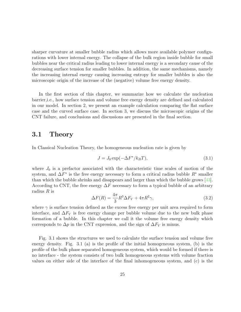
where γ is surface tension defined as the excess free energy per unit area required to forminterface, and ∆FV is free energy change per bubble volume due to the new bulk phaseformation of a bubble. In this chapter we call it the volume free energy density whichcorresponds to ∆p in the CNT expression, and the sign of ∆FV is minus.

Fig. 3.1 shows the structures we used to calculate the surface tension and volume freeenergy density. Fig. 3.1 (a) is the profile of the initial homogeneous system, (b) is theprofile of the bulk phase separated homogeneous system, which would be formed if there isno interface - the system consists of two bulk homogeneous systems with volume fractionvalues on either side of the interface of the final inhomogeneous system, and (c) is the

25

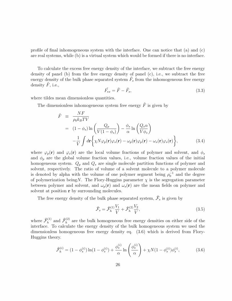
profile of final inhomogeneous system with the interface. One can notice that (a) and (c)are real systems, while (b) is a virtual system which would be formed if there is no interface.

To calculate the excess free energy density of the interface, we subtract the free energydensity of panel (b) from the free energy density of panel (c), i.e., we subtract the freeenergy density of the bulk phase separated system F̃s from the inhomogeneous free energydensity F̃ , i.e.,

F̃ex = F̃ − F̃s, (3.3)

where tildes mean dimensionless quantities.

The dimensionless inhomogeneous system free energy F̃ is given by

F̃ ≡ NF

ρ0kBTV

= (1− φs) ln

(Qp

V (1− φs)

)− φsα

ln

(Qsα

V φs

)− 1

V

∫dr

{χNϕp(r)ϕs(r)− ωp(r)ϕp(r)− ωs(r)ϕs(r)

}, (3.4)

where ϕp(r) and ϕs(r) are the local volume fractions of polymer and solvent, and φsand φp are the global volume fraction values, i.e., volume fraction values of the initialhomogeneous system. Qp and Qs are single molecule partition functions of polymer andsolvent, respectively. The ratio of volume of a solvent molecule to a polymer moleculeis denoted by alpha with the volume of one polymer segment being ρ−10 and the degreeof polymerization beingN . The Flory-Huggins parameter χ is the segregation parameterbetween polymer and solvent, and ωp(r) and ωs(r) are the mean fields on polymer andsolvent at position r by surrounding molecules.

The free energy density of the bulk phase separated system, F̃s is given by

F̃s = F̃ (1)h

V1V

+ F̃ (2)h

V2V, (3.5)

where F̃ (1)h and F̃ (2)

h are the bulk homogeneous free energy densities on either side of theinterface. To calculate the energy density of the bulk homogeneous system we used thedimensionless homogeneous free energy density eq. (3.6) which is derived from Flory-Huggins theory.

F̃ (i)h = (1− φ(i)

s ) ln(1− φ(i)s ) +

φ(i)s

αln

(φ(i)s

α

)+ χN(1− φ(i)

s )φ(i)s , (3.6)

26

0.0 0.5 1.0 1.5 2.0 2.5 3.00.0

0.2

0.4

0.6

0.8

1.0

loca

l vol

ume

frac

tions

R/Rg

polymer solvent

(a)

0.0 0.5 1.0 1.5 2.0 2.5 3.00.0

0.2

0.4

0.6

0.8

1.0

R/Rg

loca

l vol

ume

frac

tions

( V1 ) ( V2 = 1 - V1 )

(1) p

(1) s

(2) s

(2) p

polymer solvent

(b)

0.0 0.5 1.0 1.5 2.0 2.5 3.00.0

0.2

0.4

0.6

0.8

1.0

(1) p

(1) s

(2) s

(2) p

loca

l vol

ume

frac

tions

R/Rg

polymer solvent

(c)

Figure 3.1: (a) Profile of the initial homogeneous system which has initial global volumefraction values. (b) Profile of the bulk phase separated homogenous system which wouldbe formed if there was no interface. Each bulk system has volume fraction values on eitherside of interface of the inhomogeneous system. Each bulk system volume V1 and V2 aredetermined by conservation of molecules. (c) Profile of the final inhomogeneous systemafter formation of a bubble, i.e., after formation of interface

27

where φ(i)s , i = 1, 2, are solvent volume fraction values on either side of interface that would

be used to get F̃(1)h and F̃

(2)h respectively. V1 and V2 are the volumes of the homogeneous

phase separated regions given byV1 + V2 = V (3.7)

V1V

=φ(2)s − φs

φ(2)s − φ(1)

s

, (3.8)

which is derived by the conservation of total volume of solvent. Dividing the excess freeenergy by interfacial area A,the dimensionless surface tension γ is

γ̃ ≡ F̃exA

= F̃ex

(R2g

4πR2

), (3.9)

where R is the bubble radius and Rg is the radius of gyration of a polymer. Rg is the unitof length used in this thesis.

To calculate the ∆F (R) in eq.(3.2), we need to know the volume free energy density∆FV which corresponds to ∆p in CNT. ∆p in CNT is defined as the energy change due tothe phase transition of bulk inside the bubble divided by the bubble volume, which has anegative sign, i.e., the driving force of the bubble formation. Similarly, our ∆FV in eq.(3.2)is found by subtracting the homogeneous system energy from the bulk phase separatedhomogeneous system energy and dividing by the bubble volume. The dimensionless volumefree energy density ∆FV is given by

∆̃F V ≡V

V1(F̃s − F̃h), (3.10)

where F̃s is the free energy density of Fig.(3.1) panel(b) and F̃h is the free energy density ofFig.(3.1) panel(a), V and V1 are the volumes of the system and the bubble respectively. Wedefine volume V1 as the bubble volume[21], because this definition gives the same definitionof the bubble radius as CNT. The prefactor V

V 1is given by eq.(3.8).

The dimensionless free energy ∆̃F (R) necessary to form a bubble of an arbitrary radiusR is given by

∆̃F (R) = 4π

(R

Rg

)2

γ̃(R) +4π

3

(R

Rg

)3

˜∆FV (R), (3.11)

where R is radius of the bubble, i.e., radius of volume V1.

28

Alternatively, for the curved surface, we can calculate the ∆̃F (R) directly from SCFT.It is given by

∆̃F (R) =

(V (R)

R3g

)(F̃ (R)− F̃h(R)) (3.12)

We are now ready to calculate the free energy change as a function of the bubble radiusR. One should notice that the box volume is increasing as the bubble is growing, but wefix the global volume fraction values of the box. The global volume fraction values of allboxes of the bubbles need to be the same as the global volume fraction values of the initialhomogeneous system, because the bubbles we make have the same initial homogeneoussystem. Consequently our bubble is a representative bubble of our macroscopic system - inour macroscopic system, there must be many sizes of bubbles growing and shrinking, butwe can imagine one size of bubble as a representative bubble which fills in our macroscopicsystem, because the global solvent density of the system is the same as the global solventdensity of the macroscopic system.

3.2 Surface Tension, Volume Free Energy Density and

Nucleation Barrier in a Curved Surface and a Flat

Suface

We examined systems with α = 0.01, χN ranging from 120 to 160 and φs ranging from 0.2to 0.33 which is the nucleation and growth region. In this chapter, we present results of oneexample case of χN = 140 and φs = 0.23. Fig.(3.2) shows the homogeneous free energy asa function of solvent density. One can see that our system would be phase separated intoφs = 1(inside bubble) and φs = 0.16465 (outside bubble) in equilibrium.

Fig.(3.3) and Fig.(3.4) show local volume fractions of three different sizes of bubble withflat and curved surfaces, respectively. In the flat surface case, as we expected, Fig.(3.3)shows all the solvent volume fraction values outside the bubble are the same with theexpected value in Fig. (3.2) irrespective of bubble size. On the contrary, Fig.(3.4) showsthe solvent volume fraction values outside the bubble are changing depending on bubblesize, and we observe that for a smaller bubble, the solvent volume fraction value is moredeviated from the equilibrium solvent volume fraction value. Therefore, we can expectthat there must be a curvature effect in the formation of a curved surface bubble.

By using eqs.(3.8) (3.9) (3.10), we calculated the surface tension γ̃ and the volume free

energy ∆̃FV of flat and curved surface cases. For the flat surface case, we get a constant

29

0.0 0.2 0.4 0.6 0.8 1.0

-12

-10

-8

-6

-4

-2

0

2

4

6

(1)s = 1.0

Hom

ogen

eous

free

ene

rgy

s (global solvent volume fraction)

N = 140

(2)s = 0.16465

Figure 3.2: Homogeneous free energy versus global solvent volume fraction at χN = 140

30

0 1 2 3 4 50.0

0.2

0.4

0.6

0.8

1.0

R/Rg

loca

l vol

ume

frac

tions

polymer solvent

(a)

1 2 3 40.14

0.16

0.18

0.20

R/Rg

loca

l vol

ume

frac

tions polymer

solvent

(2)s = 0.16465

(b)

Figure 3.3: (a) Profiles of local volume fractions of three different sizes of bubble in theflat surface case. (b) In this blow up graph, we can see that at the outside of a bubble,three different sizes of bubble have the same solvent volume fraction value, which is theequilibrium value.

31

0 1 2 3 4 50.0

0.2

0.4

0.6

0.8

1.0

flat surface

loca

l vol

ume

frac

tions

R/Rg

polymer solvent

curved surface

(a)

1 2 3 40.14

0.16

0.18

0.20

flat surface

loca

l vol

ume

frac

tions

R/Rg

polymer solvent

curved surface

(b)

Figure 3.4: (a) Profiles of local volume fractions of three different sizes of bubble in thecurved surface case and one profile of a flat surface. (b) In this blow up graph, we can seethat in curved surface, three different sizes of bubble have different solvent volume fractionvalues at the outside of a bubble. Compared to the flat surface, in curved surface, smallerbubbles have more deviated volume fraction values from the equilibrium solvent volumefraction value. 32

0.4 0.8 1.2 1.6 2.0 2.42.6

2.8

3.0

3.2

3.4

R/Rg

dim

ensi

onle

ss s

urfa

ce te

nsio

n

curved surface flat surface

(a)

0.4 0.8 1.2 1.6 2.0 2.4

7

8

9

10

11

min

us d

imen

sion

less

vo

lum

e fr

ee e

nerg

y de

nsity

(-

F_v)

R/Rg

curved surface flat surface

(b)

Figure 3.5: (a) Surface tension values versus radius of a bubble. For curved surfaces,surface tension is decreasing for the smaller bubble in contrast to the constant value of

surface tension for the flat surface. (b) The negative of volume free energy density(−∆̃FV )

versus radius of a bubble. As the sign of ∆̃FV is minus, the sign of −∆̃FV is positive.The negative volume free energy density is increasing for smaller bubbles in contrast tothe constant value of volume free energy density for the flat surface.

33

0 0.2 0.4 0.6 0.8 1 1.2

−10

−5

0

5

10

R/Rg

∆ F

Figure 3.6: The solid line shows the free energy necessary to form a bubble of radius R(∆̃F (R)) in the flat surface case. The open circle and dotted line shows the free energy

necessary to form a bubble of radius R (∆̃F (R)) in the curved surface case.

34

value, ∆̃FV = 7.1 and γ̃ = 3.3 irrespective of bubble size, which is the expectation of CNT.However, for the curved surface case, we observe that the surface tension γ̃ and the volume

free energy density ∆̃FV are functions of bubble radius - for smaller bubbles, surface tensionis decreasing and negative volume free energy density is increasing. Fig.(3.5) shows theresults.

To calculate the dimensionless free energy ∆̃F (R) necessary to form a bubble of radiusR, for the flat surface case we used eq.(3.11) and used the constant values ˜∆FV = 7.1and γ̃ = 3.3. The solid line of Fig. (3.6) is the result of the flat surface case. For

curved surface case, we directly calculated the ∆̃F (R) using eq.(3.12). We made the boxvolume smaller until we could not find a solution which converged stably, i.e., which definedthe critical radius. We observed that below the critical radius, intermediate accuracycalculation showed the bubble is shrinking during the course of calculation. The opencircles in Fig.(3.6) is the result of the curved surface case.

From Fig. (3.6), we see that the flat surface (CNT expectation) has more than 1.5times bigger critical radius and more than 6 times bigger nucleation barrier than thecurved surface. Accordingly, our result indicates CNT predicts a much lower homogeneousnucleation rate than our results. Thus, due to the low nucleation rate expected by CNT,it has been thought that heterogeneous nucleation dominates bubble nucleation; however,our results indicate that there might be much more homogeneous nucleation possible thanpreviously thought.

3.3 Microscopic Origins of the Failure of CNT

In the previous section, our result shows much smaller nucleation barrier ∆̃F ∗ for curved

surfaces compared to the ∆̃F ∗ for flat surfaces(CNT). We noticed that for curved surfaces,

the value of surface tension γ̃ and volume free energy density ∆̃FV is a function of bubble

radius in contrast to the constant γ̃ and ∆̃FV for the flat surface. Therefore, we saw that

the variation of γ̃ and ∆̃FV as a function of bubble radius for small radius of bubbles (nano-

sized bubbles) was the reason for the significant devivation of ∆̃F ∗ for curved surfaces from

the ∆̃F ∗ of flat surfaces. We investigate the microscopic origin of the failure of CNT by

breaking down the free energy (i.e., γ̃ and ∆̃FV ) into the thermodynamic components, i.e.,internal free energy, polymer configurational entropy, polymer translational entropy, andsolvent translational entropy[36].

The below equations are used to calculate the components.

35

0.5 1 1.5 2 2.5−0.6

−0.5

−0.4

−0.3

−0.2

−0.1

0

0.1

0.2

R/Rg

dim

en

sio

nle

ss

su

rfa

ce

te

ns

ion

c

on

trib

uti

on

surface tension

polymer configurational entropy

polymer translational entropy

solvent translational entropy

internal energy

Figure 3.7: Thermodynamic components of surface tension versus bubble radius R. In-creasing polymer configurational entropy is the main cause, and the decreasing internalenergy is a secondary cause of decreasing surface tension for smaller bubbles. Below 0.9Rg, the internal energy shows a sharper decreasing.

U

ρpkBTV=χN

V

∫φp(~r)φs(r)dr (3.13)

ScpρpkBV

=1

V

∫ρp ln q(r, 1)dr +

1

V

∫ωp(r)φp(r)dr (3.14)

StpρpkBV

=1

V

∫ρp ln ρpdr, ρp = −φpV q(r, 1)

Qp

(3.15)

StsρpkBV

=φsα

ln

(Qs

φsV

)+

1

V

∫ωs(r)φs(r)dr. (3.16)

If we look at the surface tension result first, Fig. (3.7), we can see that the maincause of decreasing surface tension at smaller radii of bubbles is the increasing polymerconfigurational entropy at smaller radii. Fig.(3.8) explains why the polymer configurational

36

(a)solvent

phase

polymer

phase

Discouraged

x

Favorable

(b)

x

solvent

phase

polymer

phase

Figure 3.8: In (a) and (b) the polymer has same configuration. However, for the flatsurface (a), since the surface is flat, the polymer has more contact with solvent causinghigher internal energy. (b) In the curved surface, since the surface has curvature, thepolymer has less contact with solvent causing lower internal energy.

entropy is decreasing at the smaller radii. In Fig.(3.8) (a) and (b), one can see two polymerswhich have the same configuration. However, the polymer near curved surface has lessinteraction energy, because the polymer near curved surface has less interaction with solventmolecule due to the curvature of the surface - the solvent and polymer molecules areimmiscible.

Therefore, for bubbles with smaller radii, due to the sharper curvature of surface, thepolymer has more available configurations which have lower internal energy. Consequently,the increasing conformational entropy at higher curvatures makes the free energy decreasemore at smaller radii. And this causes the decreasing surface tension for smaller bubbles.

In addition, Fig.(3.7) shows that decreasing internal energy at higher curvatures is a sec-ondary contributor causing decreased surface tension for smaller radii bubbles. Decreasinginternal energy can be explained by the same mechanism as the increasing configurationalentropy - as explained in Fig.(3.8). Due to the higher curvature, more conformations whichhave less interaction energy are available for smaller bubble radii; accordingly the internalenergy is decreased and the surface tension decreases at smaller bubble radii.

From Fig.(3.7), we can also notice that the internal energy of surface tension decreasesmore sharply at bubbles smaller than 0.9 Rg. This is due to the disappearance of thebulk phase inside the bubble - See Fig.(3.10). Due to the collapse of the bulk phase inside

37

0.5 1 1.5 2 2.5−8

−6

−4

−2

0

2

4

6

R/Rg

dim

en

sio

nle

ss

vo

lum

e f

ree

en

erg

yc

on

trib

uti

on

volume free energy density

polymer translational entropy

solvent translational entropy

internal energy

Figure 3.9: Thermodynamic components of volume free energy density versus bubble ra-dius R. By same mechanism of surface tension, together with increasing internal energy,increasing entropy is the cause of increasing volume free energy density for smaller bubbles.

bubble, internal energy increases, i.e., there is more mixing of polymer and solvent. But,it turns out that the collapse of bulk phase inside a bubble causes a decrease of internalenergy. Since surface tension is found by subtracting the free energy of the bulk phaseseparated system from the free energy of the inhomogeneous system, and the internalenergy of the bulk phase separated system is increasing more quickly than internal energyof the inhomogeneous system, there is a sharp decrease of the internal energy at bubblessmaller than 0.9 Rg. Consequently, the collapse of the bulk phase inside the bubble appearsas a secondary cause of decreasing surface tension for smaller bubbles.

The changing volume free energy density ∆̃FV is also another cause of the small nucle-

ation barrier in curved surfaces. We broke down ∆̃FV into its thermodynamic components.Fig.(3.9) shows the result. We see the increasing entropy for smaller bubbles is a cause of

the increasing of ∆̃FV at small radii. This can be explained by the same mechanism withwhich we explained the decreasing surface tension for the small radii bubbles.

Due to the higher curvature of the surface and the collapse of the bulk phase inside the

38

0.0 0.5 1.0 1.5 2.00.0

0.2

0.4

0.6

0.8

1.0

loca

l vol

ume

frac

tions

R/Rg

polymer solvent

(a)

0 1 2 3 4 5 60.0

0.2

0.4

0.6

0.8

1.0

R/Rg

loca

l vol

ume

frac

tions

polymer solvent

(b)

0.0 0.2 0.4 0.6 0.80.0

0.2

0.4

0.6

0.8

1.0

loca

l vol

ume

frac

tions

R/Rg

polymer solvent

(c)

0 1 2 3 40.0

0.2

0.4

0.6

0.8

1.0

polymer solvent

loca

l vol

ume

frac

tions

R/Rg

(d)

Figure 3.10: (a) Profile of a critical radius of a bubble in which inside the bubble does notreach the perfect bulk phase in case of χN = 120, φs = 0.23. (b) Profile of a bubble witha perfect bulk phase inside a bubble in the case of χN = 120, φs = 0.23. (c) Profile of acritical radius of χN = 160, φs = 0.26 case. We can see a clear collapse of the bulk phaseinside the bubble. (d) To compare with (c), one profile of a bubble with perfect bulk phaseinside the bubble for the χN = 160, φs = 0.26 case.

39

0.0 0.5 1.0 1.5 2.0 2.5

-2.0

-1.5

-1.0

-0.5

0.0

0.5

1.0

dim

ensi

onle

ss s

urfa

ce te

nsio

nco

ntrib

utio

n

R/ Rg

surface tension polymer configurational entropy polymer translational entropy solvent translational entropy internal energy

Figure 3.11: Thermodynamic components of surface tension versus bubble radius R forthe case of χN = 160, φs = 0.26. Near the critical radius, at a small radius of bubble, thedecreasing internal energy becomes a main cause of decreasing surface tension for smallerbubbles.

40

bubble, there is more mixing of polymer and solvent molecules and consequently, there isincreasing internal energy for the smaller bubbles. Consequently, because of the balanceof internal energy and entropy, the entropy increases for smaller bubbles. The increasing

entropy results in increasing ∆̃FV for smaller bubbles and causes the small nucleationbarrier for curved surfaces.

In our example case, the increasing conformational entropy due to higher curvature wasthe main origin for the increasing surface tension, but for another case, χN = 160,φs = 0.26showed that the increasing internal energy due to the collapse of the bulk inside the bubbledominates the conformational entropy effect near the critical radius. Fig. (3.10)(c) showsthe volume fractions profile of the critical radius, and Fig.(3.11) shows the thermodynamiccomponents of the χN = 160, φs = 0.26 case. Thus, in the higher segregation case, theinternal energy effect might become a dominant factor though our example case in thischapter shows it as a minor origin.

3.4 Discussion and Conclusion

Considering that the flat interface assumption of CNT is not appropriate for nano-polymericbubbles, and since nano-polymeric bubbles are comparable to polymers in size, we mod-elled the surface of nano-polymeric bubbles as curved surfaces. To investigate the effect ofthe curvature on the nucleation of bubbles, we studied flat and curved surfaces by usingthe same model for both. We also compared the nucleation barrier calculated in bothcases. For the calculation of the free energy of inhomogeneous system, we used SCFT.For our example case, χN = 140, φs = 0.23 and α = 0.01, the results show that theflat surface(CNT expectation) has more than 1.5 times bigger critical radius, more than 6times bigger nucleation barrier and more than five orders smaller nucleation rate than thecorresponding values of curved surfaces.

Investigation of the microscopic origins of the failure of CNT revealed that higher curva-tures and the disappearance of the bulk phase inside bubbles causes the decreasing surfacetension and the increasing negative volume free energy density for smaller bubble. Conse-quently, there was a smaller nucleation barrier for the curved surface case. In our examplecase, the increasing conformational entropy due to higher curvature was the main originfor the increasing surface tension, but for a higher segregation case, our results showed theinternal energy effect is a dominant factor.

In conclusion, our calculation of nucleation rate for nano-polymeric bubbles using SCFTwith the assumption of curved surfaces shows much smaller nucleation barriers with the

41

smaller critical radii than predicted by CNT(flat surfaces). It turns out that the origins ofthe failure of the CNT are the assumptions of CNT which are not appropriate for nano-sized bubbles - sharp flat surfaces and bulk phases inside bubbles. Curved surface resultsshow that the high curvature and the collapse of the bulk phase inside a small bubble makesfor much smaller nucleation barriers, i.e., much bigger homogeneous nucleation rates thanCNT predicts. Thus, our results indicate that there is a much higher possibility of homo-geneous nucleation than previously thought based on CNT.

In this chapter we used an incompressible system for simplicity, but to deal with morerealistic systems, we will need to use a compressible model by using an equation of state,i.e., by incooperating pressure.

42

Chapter 4

Maximal Cell Density andTemperature Effect on Cell Density

Generally, “Good quality foam” means a foam which has a high cell density with closelyspaced and uniformly distributed small bubbles. CNT is often used to calculate cell density,but in CNT, calculation of the nucleation barrier or nucleation rates are needed to calculatethe cell density. However, as we showed in the previous chapter, CNT is not appropriatefor predicting nucleation rates for nano-cellular foams, as CNT makes assumptions that arenot applicable to nano-sized bubbles. In this chapter, we calculated the maximum possiblebubble number density directly by using SCFT without calculation of nucleation barrieror nucleation rates.

In contrast to CNT, which can only calculate nucleation rates at the critical radius,we calculated cell density as a function of bubble radius. Interestingly, our results showthat the radius of the maximal bubble surface area is different from the critical radius -it is slightly bigger than the critical radius. Also, we noticed that the bulk condition atthe center of the bubble is reached at yet another radius, which is slightly bigger than theradius of maximal surface area per unit volume. Thus, unlike CNT, we can find the upperbound maximal cell density corresponding to the critical radius, the radius of maximalbubble surface area, and the radius of the bubble with bulk condition at the center of thebubble. Thus, one can choose the “best foam” depending on the application.

On the other hand, our maximal cell density in this chapter is an upper bound on thecell density, i.e., experimentalists would get lower cell densities. However, our results can

43

qualitatively show at which experimental conditions - temperature, solvent density, ratioof solvent and polymer molecular weight, etc - experimentalists can get better foams. Weexamined maximal density in different solvent density cases at two different temperatures.Our results show that foams generally have higher maximal cell densities at lower temper-atures despite the higher surface tension at lower temperatures - contradicts with CNTprediction, since CNT predicts a higher cells density at higher temperatures because sur-face tension is lower at higher temperature. Our SCFT results also reveal that in polymericfoaming at different temperatures, the volume free energy density is a more important fac-tor than surface tension.

In the first section, we describe how we calculate bubble number density as a functionof bubble radius. In section 2, we show example results for χN = 160 - bubble numberdensity of three “best foams” in view of maximal cell density, maximal bubble surface areaper unit volume, and bulk condition at the center of a bubble at different solvent densitycases. Then, we discuss the conditions for the better foam which SCFT and CNT provideat one temperature. In section 4, we compare the results of two different temperaturecases, χN = 160 and χN = 120, and discuss the prediction of SCFT that CNT can’tprovide. In the final section, the conclusion and discussion are written.

4.1 Calculation of Bubble Number Density

In CNT,the nucleation rate is written

J = J0 exp

(−∆F ∗

kBT

)(4.1)

, where the nucleation barrier ∆F ∗ is given by

∆F ∗ =16π

3

(γ3

∆F2V

)(4.2)

Therefore, to calculate the cell density in CNT one needs to integrate the nucleationrate over time based on the nucleation barrier and also derive the prefactor J0 throughother means. We showed in the previous chapter that for high curvature surfaces, thenucleation barrier deviates from the nucleation barrier expected in CNT. Also, CNT canonly predict cell densities at the critical radius.

44

Using SCFT, we calculate the bubble number density as a function of the radius ofa bubble directly. In this chapter, we use the same inhomogeneous free energy formulaand the same model as the previous chapter. Therefore, as we described in the previouschapter, in our model, we change the size of a bubble by changing the size of the systemwhile the global volume fraction φs is held constant. In the previous chapter, since weexamined the free energy necessary to form a typical size of bubble, we had to subtractthe initial homogeneous system energy from the inhomogeneous system energy, i.e., thesystem after formation of the bubble. Since the number of molecules is conserved, we putthe global volume fraction value of the initial homogeneous system as our system globalvolume fraction value. Thus, our system global volume fraction values are the same as themacroscopic system global volume fraction values.

Therefore, our bubbles are representative bubbles of our macroscopic system,i.e., wecan think as if the macroscopic system is filled with the one representative bubble thoughin reality the macroscopic system would be filled with various sizes of bubbles. Thus, wecan calculate the bubble number density simply as the inverse of the system(box) volume.However, in this chapter, we use the cell density definition for polymer foaming, i.e., thenumber of bubbles per unit volume of polymer. Therefore, we calculate the cell density asthe inverse of the box volume times polymer volume fraction.

4.2 The ”Best” Foam

We investigated a case of χN = 160 and different global volume fraction values ranging from0.17 to 0.29, which is in the nucleation and growth region. As mentioned, we calculatedbubble number density, bubble surface area per polymer volume, and the solvent volumefraction at the center of a bubble as a function of bubble radius at each different solventvolume fraction case. Fig. 4.1 (a) shows the result of the bubble number density as afunction of radius of a bubble. It is not surprising that at the smallest radius, i.e., atthe critical radius, the foam has the maximal bubble number density. Thus, if we choosea foam which has the maximal bubble number density as the best foam, the best foamis formed at the critical radius, and we can simply get a result of Fig.4.1(b). Fig.4.1(b)shows the maximal bubble number density at different solvent volume fractions, and we seea higher cell density with increased blowing agent, which is consistent with observations.[13],[28],[19],[60],[14].

Fig. 4.2(a) shows the bubble surface area per bubble box volume as a function of bubbleradius at different solvent volume fractions. As mentioned above, surprisingly the maximal

45

0.4 0.8 1.2 1.6 2.0 2.4

0.0

0.2

0.4

0.6

0.8

1.0

1.2

S = 0.17

S = 0.20

S

= 0.23

S = 0.26

S = 0.29

cell

num

ber d

ensi

ty

R/Rg

(a)

0.3 0.4 0.5 0.6 0.7

0.0

0.2

0.4

0.6

0.8

1.0

1.2

s = 0.17s = 0.20

s = 0.23

s = 0.26

bubb

le n

umbe

r den

sity

R*/Rg

s = 0.29

(b)

Figure 4.1: At χN = 160 (a) Dimensionless bubble number density versus radius of abubble. (b) Dimensionless bubble number density at the critical radius of a bubble atdifferent solvent volume fraction systems.

46

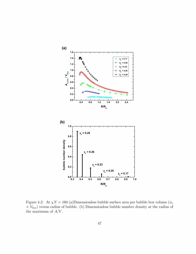
0.4 0.8 1.2 1.6 2.0 2.40.0

0.2

0.4

0.6

0.8

1.0

1.2

1.4

1.6

S = 0.17

S = 0.20

S

= 0.23

S = 0.26

S = 0.29

Abu

bble /

V box

R/Rg

(a)

0.3 0.4 0.5 0.6 0.7 0.8 0.9 1.00.0

0.2

0.4

0.6

0.8

1.0

s = 0.17s = 0.20

s = 0.23

s = 0.26

s = 0.29

bubb

le n

umbe

r de

nsity

R/Rg

(b)

Figure 4.2: At χN = 160 (a)Dimensionless bubble surface area per bubble box volume (φs× Vbox) versus radius of bubble. (b) Dimensionless bubble number density at the radius ofthe maximum of A/V .

47

surface area doesn’t occur at the critical radius - it occurs at a slightly bigger radius thanthe critical radius. Interestingly, this means that a foam which has the maximal numberdensity does not have the maximal bubble surface area. It seems that before the radiusof maximal surface area, bubble nucleation dominates the bubble growing, and after theradius of maximal surface area, the bubble growing dominates the bubble nucleation. Fig.4.2(a) shows the cell density as a function of bubble radius at different solvent volumefraction. We can see that at higher volume fraction of blowing agent, the radius of themaximal surface area is reached more quickly, so it seems that more active nucleation oc-curs with increased blowing agent. Fig. 4.2(b) shows the cell density at the radius of themaximal bubble surface area at different solvent volume fraction cases. It also shows thehigher cell density with increased solvent.

On the other hand, we examined the solvent volume fraction at the center of a bubble.Fig.(4.3)(a) is the plot of solvent volume fraction at the center of a bubble as a functionof bubble radius at different solvent volume fraction. It shows that at the critical radiusand the radius of the maximal bubble surface area, the bulk condition at the center ofa bubble was not reached. Thus, from the perspective of the quality of a bubble, at thecritical radius and the maximal surface area, the bubble quality is poor.

From the point of view of the quality of a bubble, the best foam can be defined as afoam filled with bubbles which reach the bulk condition at the center. Fig. 4.3(a) shows allpoints fall on top of each other irrespective of the global solvent density. That means thesolvent volume fraction at the center of a bubble is a function of bubble radius. We cansee that at the bubble radius R = 0.7Rg, the bulk condition is reached inside the bubbleirrespective of the global solvent density. Fig. 4.3(b) shows the bubble number density atR = 0.7Rg at different solvent volume fraction, and again this result shows a higher celldensity with increased solvent volume fraction.

For all three cases - critical radius, maximal surface area, and bulk condition at thecenter of a bubble - results show that the greater the solvent volume fraction, the higherthe cell density. However, at the critical radius case or at the maximal surface area case,the cell density was quickly increased with increased solvent volume fraction compared tothe bulk condition inside the bubble case. Also for the bubble size, at the critical radiusor at the maximal surface area cases, the bubble size is smaller with the increased blowingagent volume fraction whereas for the bulk condition at the center case, the bubble sizewas same.

Accordingly, SCFT shows several interesting results CNT can’t provide - 1) the radiusof the maximal surface area is different with the critical radius, i.e., a little bigger than the

48

0.4 0.8 1.2 1.6 2.0 2.40.80

0.84

0.88

0.92

0.96

1.00

S = 0.29

S = 0.26

S = 0.23

: S = 0.20

: S = 0.17

s at t

he c

ente

r of a

bub

ble

R/Rg

(a)

0.14 0.16 0.18 0.20 0.22 0.24 0.26 0.28 0.300.00

0.02

0.04

0.06

0.08

0.10

0.12

0.14

0.16

bubb

le n

umbe

r den

sity

s

(b)

Figure 4.3: At χN = 160 (a) Solvent volume fraction value at the center of bubbleversus radius of the bubble (b) Dimensionless bubble number density at the bubble radiusR = 0.7Rg at different solvent volume fraction systems

49

0.16

0.20

0.240.28

0.320.0

0.2

0.4

0.6

0.8

1.0

1.2

s

cel

l den

sity

Abubble/ Vsystem

cell density

bulk at center

Figure 4.4: At χN = 160, dimensionless bubble number density at different solvent volumefraction systems in view of maximal number density, maximal bubble surface area, andbulk condition at the center of a bubble.

50

0.4 0.8 1.2 1.6 2.0 2.40.5

1.0

1.5

2.0

2.5

3.0

3.5

4.0

4.5

S = 0.29

S = 0.26

S = 0.20

R/Rg

surf

ace

tens

ion

(a)

0.14 0.16 0.18 0.20 0.22 0.24 0.26 0.28 0.30 0.3212

14

16

18

20

22

24

FV

s

(b)

Figure 4.5: At χN = 160,(a) Dimensionless surface tension γ versus radius of bubble. (b)- ∆FV at R = 0.7Rg at different solvent volume fraction systems.

51

critical radius. 2) at the critical radius, and the maximal surface radius, the bulk conditionat the center of a bubble is not reached - interestingly, the solvent volume fraction is afunction of the radius of a bubble, and consequently, the radius of the bulk condition insidethe bubble is the same irrespective of the global solvent volume fraction.

Thus, if one is more interested in small bubble sizes and high bubble number densitiesrather than bubble quality, then high solvent volume fraction would be effective. But, ifone is more interested in bubble quality and the bubble size, then at the same temperature,the high solvent volume fraction would not be effective in that purpose. Even though thecell density would be still better at high solvent volume fraction, but the difference is notsignificant like at the critical radius and the maximal surface area as we can see in Fig. (4.4).

4.3 Temperature Effect on the Bubble Number Den-

sity

At mentioned above, qualitatively our SCFT results provide conditions under which abetter foam could be formed. Now, we investigate whether predictions of SCFT are qual-itatively consistent with CNT predictions. In the previous chapter, we showed that fornano-polymeric bubbles, surface tension γ and the volume free energy density ∆FV arefunctions of bubble radius whereas in CNT, γ and ∆FV are constant. Therefore, it isappropriate to compare the predictions of SCFT and CNT for cell density. First, at agiven temperature, i.e., χN = 160, we calculated surface tension γ and the volume freeenergy density ∆FV at different solvent volume fraction cases. Fig. 4.5 shows the results.Interestingly, like the solvent volume fraction at the center, all the points fall on top of eachother. This means surface tension γ is also a function of the radius of a bubble irrespectiveof the solvent volume fraction.Therefore, if we choose the good quality foam as the ”best” foam rather than the maximalcell density or maximal surface area, surface tension γ is same at different solvent vol-ume fraction. Thus, as far as γ is concerned the prediction of SCFT and CNT are same.However, for the ∆FV , our results show ∆FV increases with increasing solvent volumefraction.

Since our results show bigger ∆FV at higher solvent volume fraction,in CNT, accordingto eq. 4.2 the nucleation barrier is smaller at higher solvent volume fraction. That meanshigher nucleation and higher cell density at the higher solvent density, which is consistentwith SCFT predictions. Therefore, at a given temperature, both SCFT and CNT predic-

52

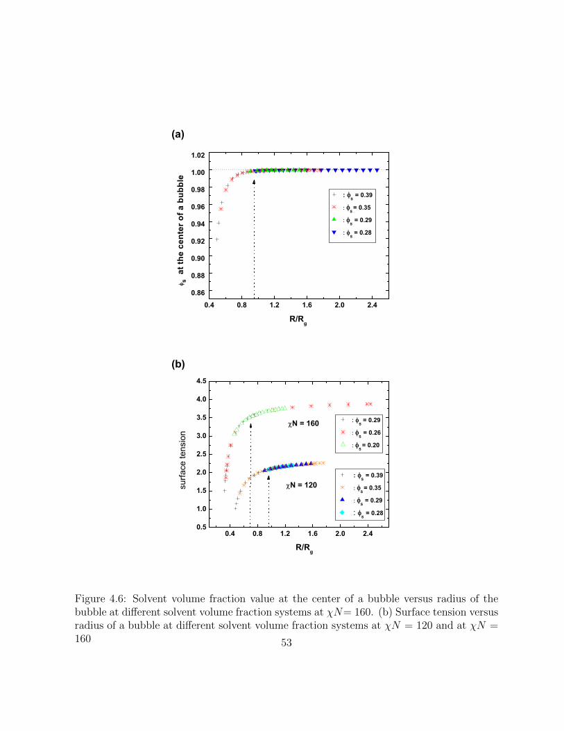
0.4 0.8 1.2 1.6 2.0 2.40.86

0.88

0.90

0.92

0.94

0.96

0.98

1.00

1.02

: S = 0.39

S = 0.35

S = 0.29

S = 0.28

s

at t

he c

ente

r of a

bub

ble

R/Rg

(a)

0.4 0.8 1.2 1.6 2.0 2.40.5

1.0

1.5

2.0

2.5

3.0

3.5

4.0

4.5

: S = 0.28

S = 0.29

S = 0.26

S = 0.20

: S = 0.39

S

= 0.35

S = 0.29

R/Rg

N = 120surfa

ce te

nsio

n

N = 160

(b)

Figure 4.6: Solvent volume fraction value at the center of a bubble versus radius of thebubble at different solvent volume fraction systems at χN= 160. (b) Surface tension versusradius of a bubble at different solvent volume fraction systems at χN = 120 and at χN =160 53

0.28 0.30 0.32 0.34 0.36 0.38 0.405.0

5.5

6.0

6.5

7.0

7.5

8.0

8.5

9.0

- F V

s

(a)

0.28 0.30 0.32 0.34 0.36 0.38 0.400.00

0.01

0.02

0.03

0.04

0.05

Bub

ble

num

ber

dens

ity

s

(b)

Figure 4.7: At χN = 120, (a) Negative volume free energy density ∆FV and (b) dimen-sionless bubble number density at different solvent volume fraction systems

54

tions are the same - higher cell density at a higher solvent volume fraction.

However, at different temperatures, we observe that SCFT reveals information whichCNT can not provide. We investigate a different temperature case, χN = 120, which isa higher temperature than χN = 160, with φs varying from 0.28 to 0.39, which is thenucleation and growth region. Like the case of χN = 160, the solvent volume fraction atthe center and surface tension are functions of bubble radius as can be seen from Fig. 4.6(a). Like the case of χN = 160, ∆FV and cell density are increasing with increased solventvolume fraction at χN = 120. Therefore, we can confirm that at a given temperature,SCFT and CNT give same information - higher cell density at a higher solvent volumefraction. However, unexpectedly at χN = 120, the bubble size at which bulk conditionsare reached at the center is R = 0.96Rg, which is bigger than the R = 0.7Rg at χN =160. We might expect at χN = 120, that the bubble size would be smaller, because as wecan see from Fig. 4.6 (b) at higher temperature, i.e., smaller χN = 120, surface tension issmaller. According to CNT, as critical radius is written as

R∗ =γ3

∆FV2 (4.3)

if γ is small, we can expect the critical radius to be small, and the radius of bulk conditionat the center of bubble to be smaller.However, we find the opposite result - a bigger bubble radius at a higher temperature.

Thus, we investigated the volume free energy density ∆FV , which is another parameterin CNT. To investigate the temperature effect, we chose the same solvent volume fractioncase for the two temperatures - φs = 0.29 at χN = 120 and χN = 160. From Fig. 4.8, we seethe bubble number density is bigger at χN = 160, low temperature, as is the bubble size.However, in Fig. 4.8(b) we see that ∆FV is bigger at the lower temperature case, χN = 160.Therefore, we can conclude that the volume free energy density ∆FV is a more dominantfactor than surface tension γ on cell density. From CNT eq.(4.2) we can predict this : ifsurface tension is smaller and volume free energy density is bigger, then the nucleationbarrier would be smaller, i.e., the cell density would be higher. But, CNT doesn’t predictwhich parameter is a more dominate factor on cell density. Fig. 4.9 (a) and (b) show bubblenumber density and ∆FV at χN = 120 and 160 at different solvent densities. Despite ofthe bigger surface tension at χN = 160, foamshaveahighercelldensityatχN = 160 exceptmuch smaller solvent density cases. Thus, our SCFT results reveal that the volume freeenergy density ∆FV is the dominant factor to make good quality, high cell density foams.Consequently, SCFT predicts that low temperature is more important than high solvent

55

0.4 0.6 0.8 1.0 1.2 1.4 1.6

0.0

0.2

0.4

0.6

0.8

1.0

1.2

N =120s = 0.29

bubb

le n

umbe

r de

nsity

R/Rg

N =160s = 0.29

(a)

0.0 0.5 1.0 1.5 2.0 2.5-25

-20

-15

-10

-5

0

N =120s = 0.29

N =160s = 0.29

F V

R/Rg

(b)

Figure 4.8: At χN = 160, φs = 0.29 and χN = 120, φs = 0.29 (a) Dimensionless bubblenumber density. (b)∆FV versus radius of bubble

56

0.150.20

0.250.30

0.350.40100

120

140160

1804

8

12

16

20

24

s

N

F V

(a)

0.150.20

0.250.30

0.350.40100

120

140160

1800.00

0.02

0.04

0.06

0.08

0.10

N

cel

l den

sity

s

(b)

Figure 4.9: At different solvent density systems at χN = 120 and χN = 160 (a) −∆FV(b) Dimensionless bubble number density

57

density for producing a good quality foam of high bubble density. These properties are notpredicted by CNT.

4.4 Discussion and Conclusion

By using a SCFT model, we directly calculated cell density as a function of bubble radiuswithout calculation of nucleation barrier and nucleation rates in CNT. Therefore, we in-vestigated the cell density in view of maximal cell density(critical radius), maximal bubblesurface area, and bulk conditions at the center of a bubble. Our examples show that themaximal cell density and maximal bubble surface area cases do not form good quality bub-bles - at the center of a bubble, bulk condition are not met - thus, we choose the best foamas the foam that has bubbles with bulk conditions at the center. By using the cell densityof the best foam at different solvent volume fractions, at a given temperature, SCFT andCNT predictions show the same trend - higher solvent volume fraction gives higher celldensity. However, at different temperatures, SCFT results reveal that at lower tempera-tures [13, 56, 55], a higher cell density is formed, despite the fact that surface tension isbigger at low temperatures. It turns out that the negative volume free energy, which ishigher at lower temperatures, contributes to the higher cell density at lower temperatures.Therefore, our SCFT results show that the volume free energy density is a more importantfactor than surface tension determining cell density of polymer foams.

In this chapter, we demonstrated that SCFT calculations show the optimal conditionssuch as temperature, chemistry, or amount of blowing agent for the formation of the bestfoams. At a given temperature, we see that CNT and SCFT prediction is same - higher celldensity at higher solvent density. However, we observed that SCFT results reveal highercell densities at lower temperatures and that volume free energy density ∆FV is a moreimportant factor than surface tensionγ for determining nucleation barriers. This is notpredicted by CNT.

Like the previous chapter, we used the incompressible system in this chapter for sim-plicity. For future work, we will need to use a compressible system which is a more realisticsystem, and confirm if the results of this chapter are qualitatively consistent with resultsof the compressible system.

58

Chapter 5

Maximal Cell Density inCompressible Systems

In this chapter, we drop the incompressible limitation we have in the previous chapters.We use a hole -based self-consistent field theory [17] to deal with a compressible system.Thus, by adding holes, our system volume expands, and our system volume is described asa function of hole volume fraction. According to our model, the representative bubble isfilled in the system, the system pressure should be the same as the representative bubblepressure. In view of a good quality foam, as a representative bubble we chose the smallestbubble of ϕs(0) ≈ 1. ϕs(0) ≈ 1 means that at the center of a bubble, the solvent volumefraction value is near 1.0, i.e., the bulk condition is reached at the center.

We calculated the inhomogeneous system pressure,homogeneous system pressure, andcell density as a function of the system volume. Inhomogeneous system is a system inwhich the representative bubbles are filled in, and homogeneous system is a system inwhich there is no bubble. Using the results we investigated not only the cell density butalso the correlation between the pressure drop rate and cell density. We also qualitativelycompared results of compressible system with the results of the incompressible system.

In the first section, we explain how the inhomogeneous system pressure is calculated.In the second section, we investigate the maximal cell density for three different processingconditions ; different temperatures with the same initial high pressure; different solventvolume fractions at the same temperature; and different temperatures with the same solventvolume fraction. Conclusions and discussion are written in the last section.

59

5.1 Theory

5.1.1 Optimal Pressure

In compressible systems, one needs to determine the system pressure at different systemvolume. At an initial high pressure, one can determine the system pressure experimentallybecause the system is in equilibrium with the outside pressure, and since the system is ho-mogeneous, one can calculate the initial pressure by using an equation of state. However,when system pressure is dropping, the system is inhomogeneous. Therefore, the systempressure is unknown, because we cannot use an equation of state to calculate the inhomo-geneous system pressure.

However, in this chapter with an assumption the system has an optimal pressure, wecalculate system pressure as a function of system volume by using our model. In ourincompressible system model in the previous chapters, the observed bubbles were the rep-resentative bubbles of the incompressible system. Since we use the same model used in thecompressible system, if we find out a representative bubble of a compressible system, thenthe representative bubble pressure should be same with the compressible system pressure.

The following is the method used to determine the optimal pressure of the inhomoge-neous system as a function of the system volume when the system volume expands withdropping pressure.

First, when the system volume expands, the system volume is described as a functionof the global hole volume fraction - by increasing the global hole volume fraction, we makethe system volume bigger. Since we assume the polymer and solvent closed packed volumesare not changed, the global polymer and solvent volume fraction values are described as afunction of the expanding system volume. As a result, the global hole volume fraction isalso a function of the expanding system volume by the constraint of the incompressibility.

If V ∗p ,V ∗s are the initial total polymer and solvent molecule closed packed volumes,V ∗p ,V ∗s are written

V ∗p = npNv∗p (5.1)

V ∗s = nsvs∗ (5.2)

, where np and ns are total number of polymer and solvent molecules respectively, N is thedegree of polymerization, and v∗p and v∗s are the closed packed polymer segment volume

60

and solvent molecule volume respectively. Therefore, V ∗p and V ∗s don’t change when thesystem volume expands. If V0 is the initial system volume, then the initial global polymervolume fraction φ0

p and initial global solvent volume fraction φ0s are written

φ0p =

V ∗pV0

(5.3)

φ0s =

V ∗sV0

(5.4)

V ∗p + V ∗s = V0 (5.5)

Then, at one specific expanded system volume Vsys,

Vsys = cV0, (c > 1) (5.6)

the global polymer, solvent, and hole volume fractions at one system volume Vsys arewritten

φp =V ∗pVsys

=V ∗pcV0

=1

cφ0p (5.7)

φs =V ∗sVsys

=V ∗scV0

=1

cφ0s (5.8)

φh =VhVsys

= 1− φp − φs (5.9)

The last eq. (5.9) obeys the relation

φp + φs + φh = 1 (5.10)

61

Therefore, the global polymer, solvent, and hole volume fraction values are functionsof system volume Vsys ( = cV0).

Second, we fix the system volume, i.e., at one constant c, we can change the cell size bychanging the bubble box volume until we get the critical cell in that fixed system volumeas we did in the incompressible system. Third, we determine a representative bubble fora specific system. As we did in the previous chapter, we choose three bubbles which givethe highest cell density, maximum bubble surface area per unit volume, and the smallestbubble with ϕs(0) ≈ 1. Then, we have three optimal pressures of the system correspond-ing to the highest cell density, the maximum bubble surface area per unit volume, and thesmallest bubble with ϕs(0) ≈ 1.

To calculate the bubble(box) pressure we use the thermodynamic pressure definition

P = −(∂F

∂V

)np,ns,T

, (5.11)

and calculate numerically.

For the numerical calculation of the pressure, we use the below equations for the valueof global volume fractions. To conserve the polymer and solvent molecules in the bubblebox, the global polymer, solvent, and hole volume fraction values at bubble box V + ∆Vare written

φp(V + ∆V ) =

(V

V + ∆V

)φp(V ) (5.12)

φs(V + ∆V ) =

(V

V + ∆V

)φs(V ) (5.13)

φh(V + ∆V ) = 1− φp(V + ∆V )− φs(V + ∆V ) (5.14)

Fig 5.1(a) shows one example plot of pressure at each system volume. Because of thescale of the plot, the pressure values looks the same in plot (a), but in plot (b), which isa blow-up figure of V = 1.1V0, we can see seven different pressure values correspondingto different sizes of bubble at V = 1.1V0. Plot (c) shows which bubble corresponds to arepresentative bubble of the highest cell density, the maximum bubble surface area perunit volume, and the smallest bubble with ϕs(0) ≈ 1.

Fig. 5.2 (a), (b) and Fig 5.3 (a) show plots of bubble density, bubble surface areaper unit volume, and solvent volume fraction at the center of a bubble respectively as a

62

1.0 1.1 1.2 1.3

100

200

300

400

500 1.001Vo

1.01 Vo

1.05 Vo

1.1 V0

1.2 V0

1.3 V0

Dim

esio

nles

s pr

essu

re

System volume (V0)

(a)

1.0 1.1 1.2 1.3185

190

195

200

1.1 V0

Dim

esio

nles

s pr

essu

re

System volume (V0)

(b)

1.0 1.1 1.2 1.3185

190

195

200

1.1 V0

Dim

esio

nles

s pr

essu

re

System volume (V0)

(c)

highest cell density

maximum A/V

s,inside ~ 1.0

Figure 5.1: (a) Plot of several bubble pressures at different system volumes. (b) Blow upof several bubble pressures at Vsys = 1.1V0. (c) Three representative bubble pressures atVsys = 1.1V0.

63

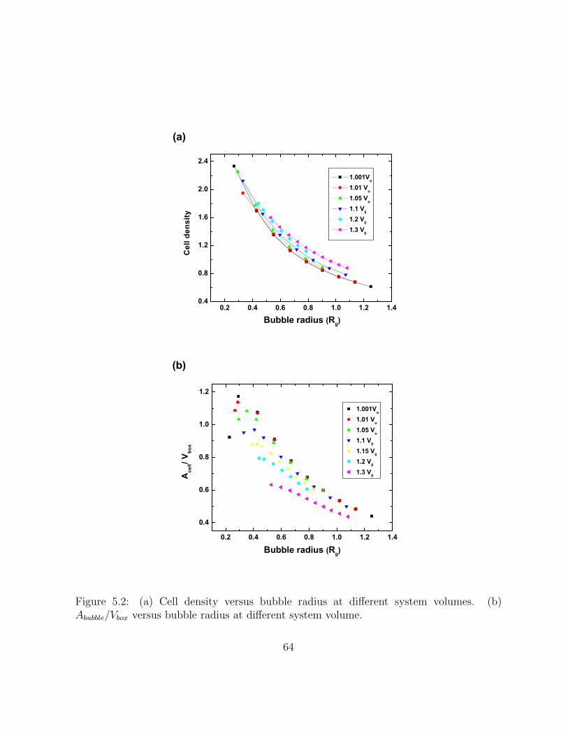
0.2 0.4 0.6 0.8 1.0 1.2 1.40.4

0.8

1.2

1.6

2.0

2.4

Bubble radius (Rg)

1.001Vo

1.01 Vo

1.05 Vo

1.1 V0

1.2 V0

1.3 V0

Cel

l den

sity

(a)

0.2 0.4 0.6 0.8 1.0 1.2 1.4

0.4

0.6

0.8

1.0

1.2

Bubble radius (Rg)

1.001Vo

1.01 Vo

1.05 Vo

1.1 V0

1.15 V0

1.2 V0

1.3 V0

Ace

ll/ Vbo

x

(b)

Figure 5.2: (a) Cell density versus bubble radius at different system volumes. (b)Abubble/Vbox versus bubble radius at different system volume.

64

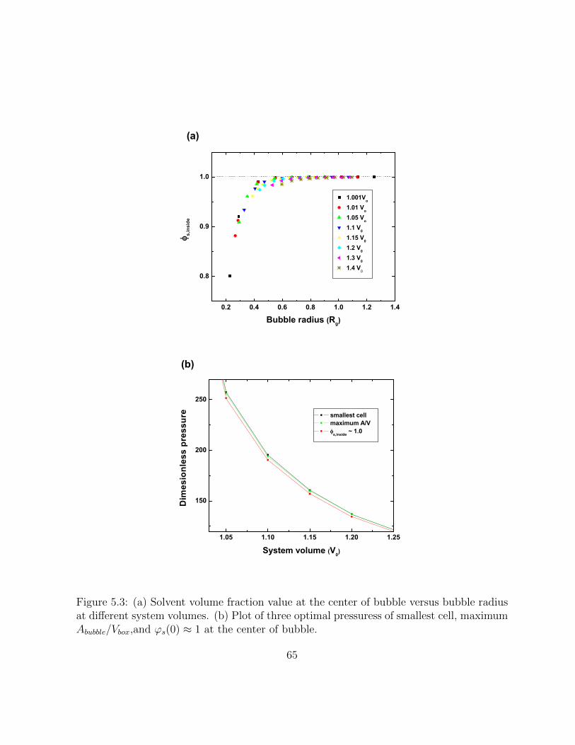
0.2 0.4 0.6 0.8 1.0 1.2 1.4

0.8

0.9

1.0

1.001Vo

1.01 Vo

1.05 Vo

1.1 V0

1.15 V0

1.2 V0

1.3 V0

1.4 V0

s,inside

Bubble radius (Rg)

(a)

1.05 1.10 1.15 1.20 1.25

150

200

250

smallest cell maximum A/V s,inside ~ 1.0

Dim

esio

nles

s pr

essu

re

System volume (V0)

(b)

Figure 5.3: (a) Solvent volume fraction value at the center of bubble versus bubble radiusat different system volumes. (b) Plot of three optimal pressuress of smallest cell, maximumAbubble/Vbox,and ϕs(0) ≈ 1 at the center of bubble.

65

function of bubble radius. We defined the radius at which the solvent and polymer volumefraction values are cross as the bubble radius. We can see from Fig. 5.2 (a) that at thecritical radius, the foam has the highest cell density. Also we can see from Fig. 5.2(b) thatat a little bigger radius than critical radius, a maximum Abubble/Vbox exists for a systemvolume just like the incompressible system. With data of Fig. 5.2 (a), (b) and Fig 5.3 (a)we plot the three optimal pressures corresponding to the highest cell density, a maximumAbubble/V and the smallest bubble with ϕs(0) ≈ 1. Fig. 5.3(b) shows one example result.

Like in the previous chapters, the cell density is calculated as the number of bubblesper unit volume of polymer, i.e., the inverse of the product of the bubble box volume timesthe global polymer volume fraction.

5.2 Maximal Cell Density

5.2.1 Different Temperature Cases with the Same Initial HighPressure

First, we examine a case of different dimensionless temperatures T = 1.5 and T = 2.0 withthe same initial high pressure. We assume a dimensionless temperature dependence foreach Flory-Huggins parameters χppN , χssN , and χpsN of

χN =A

T+B, (5.15)

where we choose App = -12, Ass = 0, Aps = 270, and all B’s as zero. We assume a weakattractive interaction between polymer molecules and a strong repulsive interaction be-tween polymer and solvent molecules. We think of the phase of the solvent as a gas phase.Therefore, for T = 1.5, the χ values are χppN = - 8, χss = 0, and χpsN = 180, and forT = 2.0, χppN = - 6, χss = 0, and χpsN = 135. For the same initial pressure, we choosethe initial solvent volume fraction φ0

s = 0.26 for T = 1.5, and φ0s = 0.31 for T = 2.0. From

the data, we observe that with our χN values, the solubility is higher at higher tempera-ture. This means our solvent is a nitrogen N2 like solvent not a carbon dioxide CO2 like,because N2 has higher solubility at higher temperature and CO2 has higher solubility atlower temperature. We will discuss this more later in the discussion and conclusions section.

Fig. 5.4 (a) shows the three optimal pressures as a function of the system volume atT = 1.5. Due to the scale of the plot, the three optimal pressure values seem the same, but

66

1.0 1.2 1.4 1.6 1.80

100

200

300

400

500

600

smallest cell maximum A/V s,inside ~ 1.0

Dim

esio

nles

s pr

essu

re

System volume (V0)

(a)

0.8 1.0 1.2390

395

400

405

smallest cell maximum A/V s,inside ~ 1.0

Dim

esio

nles

s pr

essu

re

System volume (V0)

(b)

Figure 5.4: At T = 1.5 (a) Three optimal pressures versus system volume. (b) Blow upplot of optimal pressure values at Vsys = 1.1V0.

67

1.0 1.2 1.4 1.6 1.8

0.5

1.0

1.5

2.0

2.5

System volume (V0)

Cel

l den

sity

smallest cellmaximum A/V

s,inside ~ 1.0

Figure 5.5: Three maximal cell densities corresponding to three optimal pressures versussystem volume at T = 1.5.

68

if we blow up the pressure values at 1.01 V0, in the blow-up Fig. 5.4 (b) one can see thatthe pressure of the smallest bubble is the highest and the pressure of ϕs(0) ≈ 1.0 bubbleis much lower than the smallest bubble pressure. From this, we can say that for the betterquality bubble formation, the system pressure needs to be dropped more.

Fig. 5.5 shows cell density as a function of system volume corresponding to the threeoptimal pressures. From this plot, we can easily see that at the smallest system volume,V = 1.01V0, the foam has the highest cell density for all three optimal pressures. There-fore, the incompressible system cell density must be the upper bound of the maximal celldensity for all three optimal pressures.

Also, unlike the incompressible system, Fig. 5.5 gives information on how much thesystem expand before the system is in the spinodal region. We notice that for systemsbigger than V = 1.8V0, i.e., 80% expansion, our code does not form a bubble, and thenucleation barrier approaches zero. We assume the system approaches to the spinodalregion as the nucleation barrier approaches zero.

We examine another temperature case T = 2.0 which has the same initial high pressureas the T = 1.5 case. As mentioned above, with our χN values the solubility is higher athigh temperature. For T = 2.0, φ0

s = 0.31, which is bigger than the solubility of T = 1.5case, φ0

s = 0.26.

Fig. 5.6 (a) shows the three optimal pressures for T = 2.0. If we blow up the pressuresat V = 1.01V0, Fig. 5.6 (b) shows that compared to T = 1.5 the pressure difference betweenthe smallest bubble and the ϕs(0) ≈ 1 bubble is smaller than T = 1.5 case. And, we alsonotice that the cell density difference between the smallest and the ϕs(0) ≈ 1 bubble issmaller than T = 1.5 case. In addition, like the T = 1.5case, thepressureoftheϕs(0) ≈ 1bubble is lower than the pressure of the critical radius. This means for a better qualityfoam it needs to drop more pressure, i.e. a higher pressure drop.

Fig. 5.7 shows the cell density of three optimal pressures for T = 2.0 as a functionof system volume. We also notice that at the smallest system volume the foam has thehighest cell density; thus, we conclude that the incompressible system has the upper boundmaximal cell density.

Now, to compare the two temperature cases, we choose the optimal pressure of theϕs(0) ≈ 1 bubble as the optimal pressure of a good quality foam as we did in the previouschapter. From this point, in this chapter, the optimal pressure means the optimal pressure

69

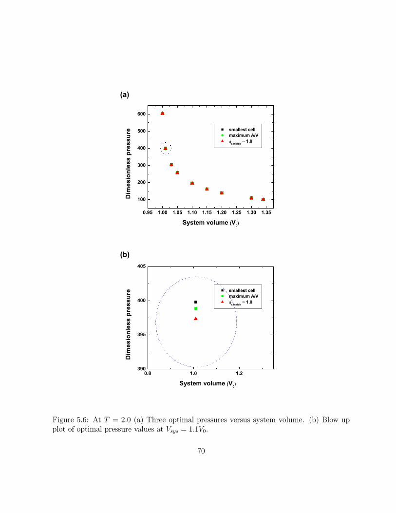
0.95 1.00 1.05 1.10 1.15 1.20 1.25 1.30 1.35

100

200

300

400

500

600

System volume (V0)

Dim

esio

nles

s pr

essu

re smallest cell maximum A/V s,inside ~ 1.0

(a)

0.8 1.0 1.2390

395

400

405

System volume (V0)

Dim

esio

nles

s pr

essu

re smallest cell maximum A/V s,inside ~ 1.0

(b)

Figure 5.6: At T = 2.0 (a) Three optimal pressures versus system volume. (b) Blow upplot of optimal pressure values at Vsys = 1.1V0.

70

1.0 1.1 1.2 1.3 1.4

0.4

0.8

1.2

1.6

smallest cellmaximum A/V

s,inside ~ 1.0

Cel

l den

sity

System volume (V0)

Figure 5.7: Three maximal cell densities corresponding to the three optimal pressuresversus system volume at T = 2.0.

71

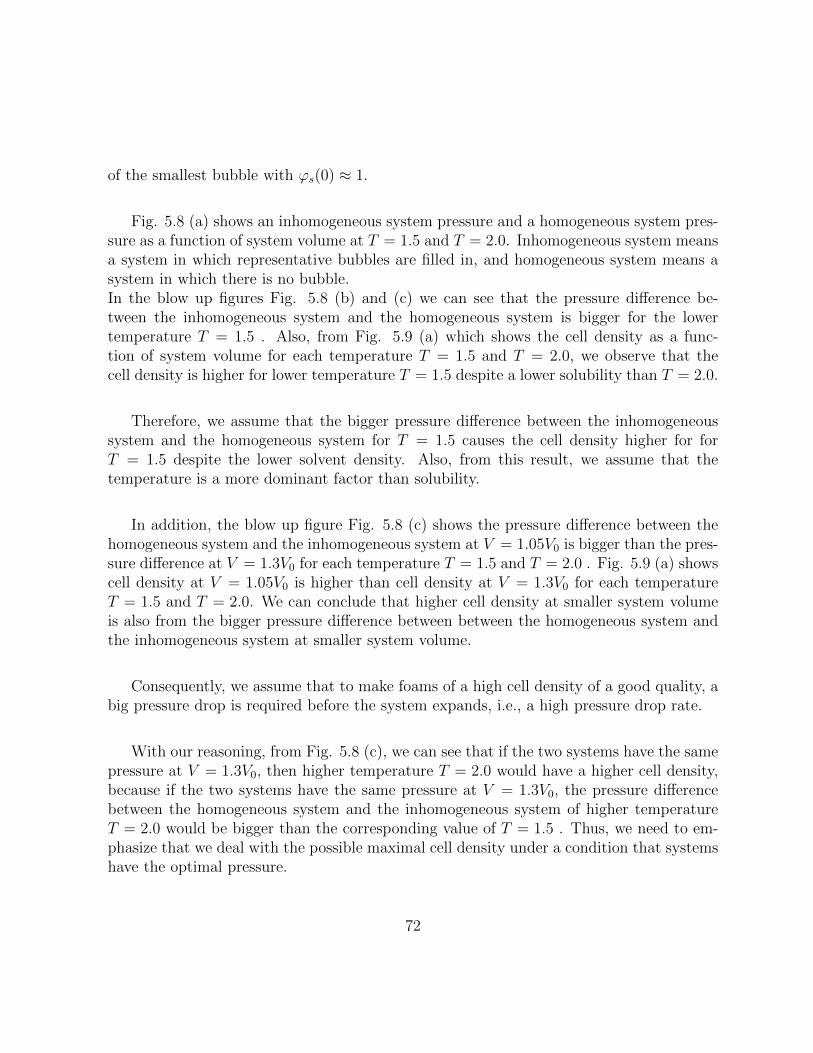
of the smallest bubble with ϕs(0) ≈ 1.

Fig. 5.8 (a) shows an inhomogeneous system pressure and a homogeneous system pres-sure as a function of system volume at T = 1.5 and T = 2.0. Inhomogeneous system meansa system in which representative bubbles are filled in, and homogeneous system means asystem in which there is no bubble.In the blow up figures Fig. 5.8 (b) and (c) we can see that the pressure difference be-tween the inhomogeneous system and the homogeneous system is bigger for the lowertemperature T = 1.5 . Also, from Fig. 5.9 (a) which shows the cell density as a func-tion of system volume for each temperature T = 1.5 and T = 2.0, we observe that thecell density is higher for lower temperature T = 1.5 despite a lower solubility than T = 2.0.

Therefore, we assume that the bigger pressure difference between the inhomogeneoussystem and the homogeneous system for T = 1.5 causes the cell density higher for forT = 1.5 despite the lower solvent density. Also, from this result, we assume that thetemperature is a more dominant factor than solubility.

In addition, the blow up figure Fig. 5.8 (c) shows the pressure difference between thehomogeneous system and the inhomogeneous system at V = 1.05V0 is bigger than the pres-sure difference at V = 1.3V0 for each temperature T = 1.5 and T = 2.0 . Fig. 5.9 (a) showscell density at V = 1.05V0 is higher than cell density at V = 1.3V0 for each temperatureT = 1.5 and T = 2.0. We can conclude that higher cell density at smaller system volumeis also from the bigger pressure difference between between the homogeneous system andthe inhomogeneous system at smaller system volume.

Consequently, we assume that to make foams of a high cell density of a good quality, abig pressure drop is required before the system expands, i.e., a high pressure drop rate.

With our reasoning, from Fig. 5.8 (c), we can see that if the two systems have the samepressure at V = 1.3V0, then higher temperature T = 2.0 would have a higher cell density,because if the two systems have the same pressure at V = 1.3V0, the pressure differencebetween the homogeneous system and the inhomogeneous system of higher temperatureT = 2.0 would be bigger than the corresponding value of T = 1.5 . Thus, we need to em-phasize that we deal with the possible maximal cell density under a condition that systemshave the optimal pressure.

72

1.0 1.2 1.4 1.6 1.8 2.00

100

200

300

400

500

600

700

(a)

Dim

ensi

onle

ss p

ress

ure

System volume (V0)

- pressure of inhomogeneous system

- pressure of homogeneous system

T = 1.5 ( s=0.26) T = 2.0 ( s=0.31)

T = 1.5 ( s=0.26)T = 2.0 ( s=0.31)

1.050

250

255

260

- pressure of inhomogeneous system

T = 1.5 ( s=0.26) T = 2.0 ( s=0.31)

T = 1.5 ( s=0.26) T = 2.0 ( s=0.31)

- pressure of homogeneous system

System volume (V0)

Dim

ensi

onle

ss p

ress

ure

(b)

1.300100

105

110

115

- pressure of inhomogeneous system

T = 1.5 ( s=0.26) T = 2.0 ( s=0.31)

T = 1.5 ( s=0.26) T = 2.0 ( s=0.31)

- pressure of homogeneous system

System volume (V0)

Dim

ensi

onle

ss p

ress

ure

(c)

Figure 5.8: At T = 1.5 and T = 2.0 (a) Pressure of the inhomogeneous system and thehomogeneous system versus system volume (b) Blow up plot of the pressure at V = 1.05V0.(c) Blow up plot of the pressure at V = 1.3V0.

73

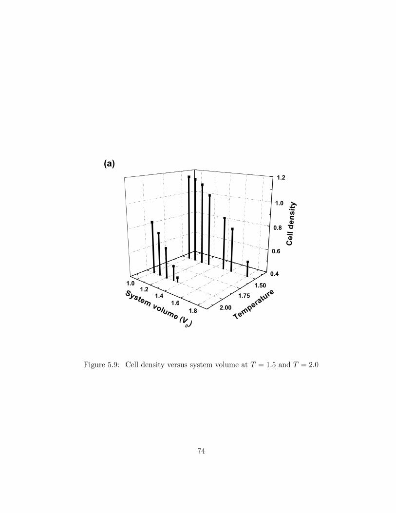
1.501.75

2.00

1.01.2

1.41.6

1.8

0.4

0.6

0.8

1.0

1.2

Cel

l den

sity

Temperature System volume (V0 )

(a)

Figure 5.9: Cell density versus system volume at T = 1.5 and T = 2.0

74

On the other hand, we also see that at lower temperature, the system expands more.We assume that the initial higher cell density at lower temperature causes the system vol-ume expand more.

5.2.2 Different Solvent Density Cases at the Same Temperature

In the previous chapter, we examined different solubility cases (different solvent volumefraction cases) at the same temperature. To check in the compressible system if we getthe same result as the incompressible system, we examined different solubility cases at thesame temperature in this section. We used the same parameter values as the incompress-ible system, χN = 120 ( χppN = - 6, χssN = 0, χpsN = 117 ) with φs ranging from 0.32 to0.39.

Fig. 5.10 shows the optimal pressure of ϕs(0) ≈ 1 bubble as we mentioned above, as wecan expect, despite of the scale of the plot we see that the highest solubility φs = 0.39 hasthe highest initial high pressure. The blow up Fig. 5.10 (b) and (c) show that the pressuredifference from the homogeneous system is bigger for higher solvent density. Therefore, weexpect a higher solvent case would have a higher cell density.

Fig. 5.11 shows the results of the cell density of the three solubility cases as a functionof system volume. As we expect, a higher solvent case has a higher cell density, and alsoexpands more in a higher solvent case.

Thus, we can conclude that for the different solvent density cases at the same temper-ature, the compressible system result is the same as the incompressible result - a highercell density at a higher solubility.

In addition, from Fig. 5.10 (a),(b) and Fig. 5.11, we can see

5.2.3 Different Temperature Cases with the Same Solvent Vol-ume Fraction

As we did in the previous chapter, to investigate the effect of temperature on cell density,we examine different χN value cases, i.e., χN = 120 (χppN = - 6, χssN = 0, χpsN = 117)

75

1.0 1.1 1.2 1.30

100

200

300

400

500

600

700

- pressure of inhomogeneous system

s = 0.39 s = 0.35 s = 0.32

s = 0.39 s = 0.35 s = 0.32

Dim

ensi

onle

ss p

ress

ure

System volume (V0)

(a)

- pressure of homogeneous system

1.050255

260

265

270

- pressure of inhomogeneous system

s = 0.39 s = 0.35 s = 0.32

s = 0.39 s = 0.35 s = 0.32

Dim

ensi

onle

ss p

ress

ure

System volume (V0)

(b)

- pressure of homogeneous system

1.100190

195

200

205

210

- pressure of inhomogeneous system

s = 0.39 s = 0.35 s = 0.32

s = 0.39 s = 0.35 s = 0.32

Dim

ensi

onle

ss p

ress

ure

System volume (V0)

(c)

- pressure of homogeneous system

Figure 5.10: At different solvent volume fractions (solubilities) for χN = 120 (a) Pressureof the inhomogeneous system and the homogeneous system versus system volume (b) Blowup plot of the pressure V = 1.05V0. (c) Blow up plot of the pressure at V = 1.1V0

76

0.320.34

0.360.38

0.40

0.5

0.6

0.7

0.8

0.9

1.0

1.0

1.11.2

1.31.4

Cel

l den

sity

System volume(V 0)

Solvent density (s )

Figure 5.11: Cell density versus system volume at different solvent volume fractions (sol-ubilities) for χN = 120

77

and χN = 160 (χppN = - 8, χssN = 0, χpsN = 156) with the same solvent volume fractionφs = 0.32. Fig. 5.12 (a) shows the optimal pressure of the two cases and the correspondinghomogeneous system pressure as a function of system pressure. We see at χN = 160, thelow temperature case needs higher pressure to have the same solubility as the χN = 120,high temperature, as we expect. In figure Fig. 5.12 (b) we see a much bigger pressuredifference between the inhomogeneous system pressure and the homogeneous system pres-sure at χN = 160. Thus, we can expect a much bigger higher cell density at χN = 160which we can see in Fig. 5.13 (a). Also, though we didn’t calculate a bigger system casethan 1.3V0 for χN = 160, we see more expansion at χN = 160.

Consequently, for the different temperature cases with the same solvent volume fraction,we also get the same result as the incompressible system - low temperature has a higher celldensity. In addition, we see also a bigger volume expansion at χN = 160, low temperature.We assume that this is from the higher cell density due to the bigger pressure differencebetween the inhomogeneous system pressure and homogeneous system pressure at thesmallest system volume for χN = 160.

5.3 Discussion and Conclusion

In this chapter, we chose the optimal pressure of φs(0) ≈ 1 bubble as the system pressure,and calculated pressure of inhomogeneous system and the homogeneous system, cell den-sity as a function of system volume.

Our compressible system prediction of cell density shows that the incompressible sys-tem cell density is the upperbound of the maximal cell density. Thus, in view of celldensity the compressible system predictions are consistent with the incompressible systempredictions - Low temperature and high solvent volume fraction have a higher maximalcell density[47, 41].

We noticed that when the system expands, the nucleation barrier approaches zero,and our code doesn’t form a bubble as the nucleation barrier approaches to zero . (around∼ 10−3) We assume the system approaches the spinodal region when the nucleation barrierapproaches zero.

We investigated three cases - different temperatures with the same initial high pressure;different solvent volume fraction at the same temperature; and different temperatures with

78

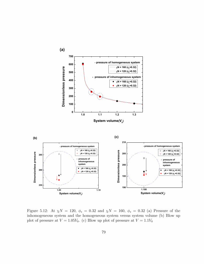
1.0 1.1 1.2 1.30

100

200

300

400

500

600

700

- pressure of inhomogeneous systemN = 160 ( s=0.32) N = 120 ( s=0.32)

- pressure of homogeneous system

N = 160 ( s=0.32) N = 120 ( s=0.32)

Dim

ensi

onle

ss p

ress

ure

System volume(V0)

(a)

1.05 1.10

255

260

265

- pressure of inhomogeneous system

N = 160 ( s=0.32) N = 120 ( s=0.32)

- pressure of homogeneous system

N = 160 ( s=0.32) N = 120 ( s=0.32)

Dim

ensi

onle

ss p

ress

ure

System volume(V0)

(b)

1.100190

195

200

205

210

(c)

- pressure of inhomogeneous system

N = 160 ( s=0.32) N = 120 ( s=0.32)

N = 160 ( s=0.32) N = 120 ( s=0.32)

- pressure of homogeneous system

System volume(V0)

Dim

ensi

onle

ss p

ress

ure

Figure 5.12: At χN = 120, φs = 0.32 and χN = 160, φs = 0.32 (a) Pressure of theinhomogeneous system and the homogeneous system versus system volume (b) Blow upplot of pressure at V = 1.05V0. (c) Blow up plot of pressure at V = 1.1V0

79

100120

140160

180

0.4

0.6

0.8

1.0

1.2

1.4

1.0

1.11.2

1.31.4

System volume (V 0)

Cel

l den

sity

N

Figure 5.13: Cell density versus system volume at χN = 120, φs = 0.32 and χN = 160,φs = 0.32.

80

the same solvent volume fraction.

Commonly for all cases, our results show that the highest cell density occurs at thesmallest system. And, bigger pressure difference between the homogeneous system and theinhomogeneous system makes higher cell density. Therefore, to make foams of the high celldensity with good quality bubbles, high pressure dropping rate is required. [45, 67, 46].And, also our result - high cell density at low temperature and high cell density for a highpressure drop rate - is similar with carbon dioxide case. Thus, since usually in experimentsof nitrogen solvent the solubility is very small, by using a higher χps and lower solubility,we can compare the results with the experimental results of nitrogen case - there is littleeffect of temperature and pressure drop rate on cell density.

On the other hand, by raising the pressure we can increase solubility with the sametemperature or lower temperature with same solubility. Our results show lowering temper-ature is a more efficient way to get a better quality foam than increasing solubility, whichis consistent with the result of the previous chapter - temperature is a dominant factor.

As for the solubility, according to our investigation, with magnitude of χps smallerthan half the magnitude of χpp or if χps has minus sign, the solubility has higher at lowertemperature which is a character of the solubility of CO2 [52]. However, our code does notmake a cell if we use above parameter values. Thus, to investigate the CO2 case, we mightneed to use the Simha -Chomkynsky eq. in which a van der Waals interaction potentialused. Or a modified Sanchez -Lacombe eq. can be used by setting polymer segment volumeand hole volume differently, i.e., v∗p 6= v∗h.

81

Chapter 6

Conclusions

We studied cell nucleation and growth in nano polymer foams in this thesis. For the calcu-lation of the inhomogeneous polymer system free energy we used self-consistent field theory(SCFT).

As our research is about nano-sized bubbles, which are comparable in size to polymermolecules, we represented a bubble surface as a curved surface, and investigated the cur-vature effect on cell nucleation. Unlike classical nucleation theory (CNT), in which valuesof surface tension γ and volume free energy density ∆FV are constant, our results showthat surface tension γ is decreasing and (negative) volume free energy density, −∆FV , isincreasing for smaller bubbles (higher curvature). We investigated the microscopic originsof the decreasing surface tension γ and increasing (negative) volume free energy density−∆FV at smaller bubbles by breaking down the components of free energy. It turns outthat the higher curvature of small bubbles gives polymer molecules more available config-urations leading to the lower internal energy, and also the bulk phase breakdown insidesmaller bubbles decreases the internal energy. Consequently, our SCFT results show thatnano-polymeric bubbles have a much smaller nucleation energy, i.e., a much larger nucle-ation rate than predicted by CNT ; therefore, we can expect a much higher possibility ofhomogeneous nucleation than previously calculated by CNT.

In our model, each bubble we make is a representative bubble of each correspondingsample system. With our model, we directly calculated the maximal cell density as afunction of bubble radius without calculation of nucleation barrier and nucleation ratesin CNT. We investigated under what conditions of parameters such as temperature and

82

solvent density better foams might be formed in view of cell density and cell size. Ourresults show that at one given temperature, CNT and SCFT predictions are the same -better foam at higher solvent density. However, for different temperatures, SCFT predic-tions show that a better foam (higher cell density and smaller cell size) is formed at lowertemperatures despite lower solvent density, and it turns out that the free volume energydensity,∆FV , is a more dominant factor than surface tension γ for cell density and criticalcell size predictions. This is not revealed by CNT.

We calculated the maximal density in compressible systems as well as the incompress-ible system. We used hole-based SCFT for compressible system calculations. With anassumption that our system has an optimal pressure at which the system has the maximalcell density with a good quality bubble, i.e., bulk condition inside a bubble, we calculatedinhomogeneous system pressure, homogeneous system pressure, maximal cell density, ex-pansion ratio, and void fraction as functions of system volume.We observed that when system volume expands nucleation barrier approaches to zero, andwe couldn’t make a bubble when the nucleation barrier is very small. Thus, we assumedthat when the nucleation barrier approaches to zero, system approaches to spinodal re-gion, and we assumed the biggest system volume which we could make is the final systemvolume.

Therefore, with data of cell density, pressure, expansion ratio, and void fraction wecould investigate maximal density, expansion ratio and cell morphology of the final sys-tem depending on different processing conditions - different temperatures with same initialhigh pressure, different solvent density cases at the same temperature, and different tem-peratures with same solvent volume fraction. First of all, our results showed that theincompressible maximal cell density is the upper bound of the maximal cell density, andqualitatively consistent with the compressible prediction; higher cell densities at lower tem-peratures and higher solvent densities.Our compressible systems also showed higher expansion ratio at low temperature and highsolvent densities. Since we noticed that the pressure difference between homogeneous sys-tem and inhomogeneous system is bigger at low temperature and high solvent cases, weconcluded that the bigger pressure difference between homogeneous system and inhomo-geneous system must cause the higher cell density, and the initial higher cell density mustcause the bigger final system volume. We also observed that for all our results, the smallestvolume has the highest cell density, thus; big pressure drop rate is required for high celldensity of good quality foams.

In addition, though higher solubility and low temperature make a higher cell density,

83

our results showed temperature is a more dominant factor for a higher cell density. Fromone system if we can raise solubility or lower temperature by raising a same amount of theinitial pressure, it turns out that raising temperature is more efficient to make a higher celldensity of good quality foam, but a bigger pressure drop rate was required.

On the other hand, overall our void fraction values were high since our system hasa high solubility. And, though our solvent type is nitrogen since with our χ values, ourcompressible system has higher solvent density at higher temperature[52], our results weresimilar with the carbon dioxide results - significant effect of temperature and pressure droprate on cell density. In experiments using nitrogen, usually the solubility is very small, andresults show little effect of temperature and pressure drop rate on cell density[25].

Therefore, for future work, we can use bigger χps and smaller solubility, and comparethe results with the experimental results, i.e., the extent of the effect of processing condi-tion on cell density.In addition, we observed that if the magnitude of repulsive force between polymer andsolvent,χps, was approximately smaller than half the magnitude of attractive force be-tween polymer molecules χpp or if repulsive force between polymer and solvent, χps, wasnegative, then the solubility is higher at lower temperatures, which is a character of thesolubility of carbon dioxide. If we use the range of above χps values, our code didn’t makea bubble. We assume the pair wise contact potential of the molecules interaction of ourmodel might cause the incapability for the carbon dioxide case. According to our investi-gation of χps values, the repulsive force of carbon dioxide and polymer molecules must bemuch smaller than the repulsive force of nitrogen and polymer molecules. thus; interactionrange between carbon dioxide and polymer molecules must be bigger. Therefore, for theinvestigation of the solvent carbon dioxide case, we might need to use the Simha - Som-cynsky equation[54, 20], because in Simha - Somcynsky equation, van der Waals potentialwhich has a longer attractive interaction range than our model is used.

On the other hand, in our model, by setting the closed packed polymer segment volumeis equal to hole volume, our code was based on Sanchez -Lacombe equation, but we mightuse a modified Sanchez -Lacombe equation [51, 23] by setting the closed packed polymersegment volume and hole volume differently,i.e., v∗p 6= v∗h.

Furthermore, we noticed that our results showed different homogeneous system pressurefor different χ values, thus; we might investigate effects of different χ or α values on foams

84

quality. And, our calculation was qualitative calculation, but quantitative calculation andcomparison with experiment would give more insight about bubble nucleation and growthmechanisms.

85

Permissions

This is a License Agreement between Yeongyoon Kim (”You”) and Elsevier (”Elsevier”)provided by Copyright Clearance Center (”CCC”).

Supplier : Elsevier LimitedThe Boulevard,Langford LaneKidlington,Oxford,OX5 1GB,UKRegistered Company Number : 1982084Customer name : Yeongyoon KimCustomer address : 314 BWaterloo, ON N2L 6P4License number : 3016000076124License date : Oct 25, 2012Licensed content publisher : ElsevierLicensed content publication : PolymerLicensed content title :Towards maximal cell density predictions for polymeric foamsLicensed content author :Yeongyoon Kim,Chul B. Park,P. Chen,Russell B. ThompsonLicensed content date : 10 November 2011Licensed content volume number : 52Licensed content issue number : 24Number of pages : 8Start Page : 5622End Page : 5629Type of Use : reuse in a thesis/dissertationIntended publisher of new work : otherPortion : full article

86

Format : electronicAre you the author of this Elsevier article? : YesWill you be translating? : NoOrder reference numberTitle of your thesis/dissertation :Study of cell nucleation in nano polymer foams : SCFT approachExpected completion date : Oct 2012Estimated size (number of pages) : 91Elsevier VAT number : GB 494 6272 12Permissions price : 0.00 USDVAT/Local Sales Tax : 0.0 USD / 0.0 GBPTotal : 0.00 USD

87

References

[1] M. Amon and C. D. Denson. A study of the dynamics of foam growth: Analysis ofthe growth of closely spaced spherical bubbles. Polym. Eng. Sci., 24(13):1026–1034,1984.

[2] D. F. Baldwin, D. Tate, Park. C. B., S. W. Cha, and N. P. Suh. Microcellular plasticsprocessing technology (1). J. Jpn. Soc. Polym. Proc., 6:187, 1994.

[3] D. F. Becker and W. Doring. Ann. Phys., 24:719, 1935.

[4] K. Binder, M Muller, P. Virnau, and L. G. MacDowell. Polymer + Solvent sys-tems:phase diagrams, interface free energy, and nucleation. Adv. Polym. Sci., 173:1,2005.

[5] J. S. Colton and N. P. Suh. The nucleation of microcellular thermoplastic foam withadditives: Part 2: Experimental results and discussion. Polym. Eng. Sci., 27(7):493–499, 1987.

[6] J. S. Colton and N. P. Suh. The nucleation of microcellular thermoplastic foam withadditives: Part 1:Theoretical consideration. Polym. Eng. Sci., 27(7):485–492, 1987.

[7] A. Das. Field Theory: A path integral approach. World Scientic, Singapore, 2006.

[8] G. T. Dee and B. B. Sauer. The molecular weight and temperature dependence ofpolymer surface tension: Comparison of experiment with interface gradient theory. J.Colloid. Interf. Sci., 152:85–103, 1992.

[9] G. T. Dee and B. B. Sauer. The surface tension of polymer liquids. Adv. Phys.,47:161–205, 1998.

[10] G. H. Fredrikson. The equilibrium theory of inhomogeneous polymers. Oxford Univer-sity Press, New York, 2006.

88

[11] Y. Fujimoto, S. S. Ray, and M. Okamoto. Well controlled biodegradable nano-composite foams: from microcellular to nanocellular. Macromol. Rapid Comm.,24:457–461, 2003.

[12] S. Ghosh and S. K. Ghosh. Homogeneous nucleation in vapor-liquid phas transi-tion of Lennard-Jones fluids: A density functional theory approach. J. Chem. Phys.,134(024502):1–8, 2011.

[13] S. K. Goel and E. J. Beckman. Generation of microcellular polymeric foams usingsupercritical carbon dioxide. 1: Effect of pressure and temperature on nucleation.Polym. Eng. Sci., 34(14):1137–1147, 1994.

[14] X. Han, K. W. Koelling, D. L. Tomasko, and L. J. Lee. Continuous microcellularpolystrene foam extrusion with supercritical study. Polym. Eng. Sci., 42:2094–2106,2002.

[15] M. M. Hasan, Y. G. Li, G. Li, C. B. Park, and P. Chen. Determination of solubilitiesof CO2 in linear and branched polypropylene using a magnetic suspension balanceand a PVT apparatus. J. Chem. Eng. Data, 55:4885–4895, 2010.

[16] Eugene Helfand. Theory of inhomogeneous polymers: Fundamentals of the Gaussianrandom-walk model. J. Chem. Phys., 62:999–1005, 1995.

[17] K. Hong and J. Noolandi. Conformational energy effects in a compressible lattice fluidtheory of polymers. Macromolecules, 14:1229–1234, 1981.

[18] K. Hong and J. Noolandi. Theory of inhomogeneous multicomponent polymer systems.Macromolecules, 14:727–736, 1981.

[19] S. Ito, K. Matsunaga, M. Tajima, and Y. Yoshida. Generation of microcellular polyure-tane with supercritical carbon dioxide. J. Appl. Polym. Sci., 106:3581–3586, 2007.

[20] R. K. Jain and R. Simha. On the statistical thermodynamics of multicomponentfluids: Equation of state. Macromolecule, 13(6):1501, 1980.

[21] R. A. L. Jones and R. W. Richards. Polymers at Surfaces and Interfaces. CambridgeUniversity Press, Cambridge, 1999.

[22] B. Krause, Dickmann K., van der Vegt, and Wessling N. F. A. Open nanoporousmorphologies from polymeric blends by carbon dioxide foaming. Macromolecules,35:1738–1745, 2003.

89

[23] R. H. Lacombe and I. C. Sanchez. Statistical thermodynamics of fluid mixtures. J.Phys. Chem., 80(23):2568, 1976.

[24] J. G. Lee and R. W. Flumerfelt. A refined approach to bubble nucleation and polymerfoaming process: Dissolved gas and cluster size effects. J. Colloid Interf. Sci., 184:335–348, 1994.

[25] J. W. S. Lee and C. B. Park. Use of nitrogen as a blowing agent for the production offine-celled high-density HDPE foams. Macromol. Mater. Eng., 291:1233–1244, 2006.

[26] S. T. Lee, B. C. Park, and N. S. Ramesh. Polymeric Foams: Science and Technology.CRC press, Boca Raton, 2007.

[27] D. G. LeGrand and G. L. Gains. The molecular weight dependence of polymer surfacetension. J. Colloid. Interf. Sci., 31:162–167, 1969.

[28] S. N. Leung, A. Wong, Q. Guo, C.B. Park, and J. H. Zong. Change in the criticalnucleation radius and its impact on cell stability during polymeric foaming process.Chem. Eng. Sci., 64:4899–4907, 2009.

[29] S. N. Leung, A. Wong, C. B. Park, and Q. Guo. Strategies to estimate the pressuredrop threshold of nucleation for polystyrene foam with carbon dioxide. Ind. Eng.Chem. Res., 48:1921–1927, 2002.

[30] G. Li, J. Wang, C. B. Park, P. Moulinie, and R. Simha. Comparison of ss-based andsl-based estimation of gas solubility. ANTEC2004, pages 2566–2575, 2004.

[31] G. Li, J. Wang, C. B. Park, and R. Simha. Measurement of gas solubility in lin-ear/branched PP melts. J. Polym. Sci. Pol. Phys., 45:2497–2508, 2007.

[32] L. Li, H. Yokoyama, T. Nemoto, and K. Sujiyama. Facile fabrication of nanocellularblock copolymer thin films using supercritical carbon dioxide. Adv. Mater., 16:1226–1229, 2004.

[33] J. Matini, F. A. Waldman, and N. P Suh. The production and analysis of microcellularthermoplastic foams. SPE ANTEC Technol. paper, 28:674, 1982.

[34] M. W. Matsen. The standard gaussian model for block copolymer. J. Phys-CondensMat., 14:R21–R47, 2002.

[35] M. W. Matsen. Self-consistent field theory and its appilcation. Soft Matter, 1:1–84,2006.

90

[36] M. W. Matsen and F. S. Bates. Block copolymer microstructures in the intermediate-segregation regime. J. Chem. Phys., 106:2436–2448, 1997.

[37] L. M Matuana and C. A. Diaz. Study of cell nucleation in microcellular poly(lacticacid)foamed with supercritical CO2 through a continuous-extrusion process. Ind. Eng.Chem. Res., 49:2186–2193, 2010.

[38] J. Merikanto, E. Zapadinsky, A. Lauri, and H. Vehkamaki. Origin of the failure ofclassical nucleation theory: incorrect description of the smallest clusters. Phy. Rev.Lett., 98(145702):1–4, 2007.

[39] M. Muller, L. G. MacDowell, P. Virnau, and K. Binder. Interface properties andbubble nucleation in compressible mixtures containing polymers. J. Chem. Phys.,117:5480, 2002.

[40] H. E. Naguib, C. B. Park, and P. C. Lee. Effect of Talc content on the volumeexpansion behavior of extended PP foams. J. Cell. Plast., 39:499, 2003.

[41] H. E. Naguib, C.B. Park, and N. Reichelt. Fundamental foaming mechanics gov-erning the volume expansion of extruded polypropylene foam. J. Appl. Polym. Sci.,91(4):2661–2668, 2004.

[42] V. Neimark and A. Vishnyakov. Monte carlo simulation study of droplet nucleation.J. Chem. Phys., 122(145702):1–11, 2005.

[43] D. W Oxtoby. Density functional methods in the statistical mechanics of materials.Annu. Rev. Mater. Res., 32:39–52, 2002.

[44] D. W. Oxtoby and R. Evans. Nonclassical nucleation theory for the gas-liquid tran-sition. J. Chem. Phys., 89:7529, 1988.

[45] C. B. Park, D. F. Baldwin, and N. P. Suh. Effect of pressure drop rate on cell nucleationin continuous processing of microcellular polymers. Polym. Eng. Sci., 35:432, 1995.

[46] C. B. Park and N. P. Suh. Filamentary extrusion of microcellular polymers using arapid decompressive element. Polym. Eng. Sci., 36:34, 1996.

[47] C.B. Park, A.H. Behravesh, and R.D. Venter. Low density, microcellularfoam pro-cessing in extrusion using CO2. Polym. Eng. Sci., 38(11):1812–1823, 1998.

91

[48] H. Park, R. B. Thompson, N. Lanson, C. Tzoganakis, C. B. Park, and P. Chen. Effectof temperature and pressure on surface tension of polystyrene in supercritical carbondioxide. J. Phys. Chem., 111:3859, 2007.

[49] E. Parra and J. C. Grana. Influence of the attractive pair-potential in density func-tional models of nucleation. J. Chem. Phys., 132(034702):1–9, 2010.

[50] B Rathke. Blasenbidung in gasgesattigten Flussigkeiten: Der Nachweis homogenerKeimbidung. Fortschritt-Berichte, 3:770, 2003.

[51] I. C. Sanchez and R. H. Lacombe. An elementary molecular theory of classical fluids.Pure fluids. J. Phys. Chem., 80(21):2352, 1976.

[52] Y. Sato, M. Yurugi, K. Fujiwara, S. Takishima, and H. Masuoka. Solubilities of carbondioxide and nitrogen in polystyrene under high temperature and pressure. Fluid PhaseEquilibr., 125:129–138, 1996.

[53] S. Schukla and K. W. Koelling. Classical nucleation theory applied to homogeneousbubble nucleation in the continuous microcellular foaming of the polystyrene-co2 sys-tem. Ind. Eng. Chem. Res., 48:7963–7615, 2009.

[54] R. Simha and T. Somkynsky. On the statistical thermodynamics of spherical andchain molecule fluids. Macromolecules, 2:342, 1969.

[55] V. Talanquer, C. Cunningham, and D. W. Oxtoby. Bubble nucleation in binarymixtures: A semiempirical approach. J. Chem. Phys., 114:6759–6762, 2001.

[56] V. Talanquer and D. W. Oxtoby. Nucleation of bubbles in binary fluids. J. Chem.Phys., 102:2156–2164, 1995.

[57] R. B. Thompson, J. R. MacDonald, and P. Chen. Origin of change in molecular-weightdependence for polymer surface tension. Phys. Rev. E, 78:030801, 2008.

[58] R. B. Thompson, C. B. Park, and P. Chen. Reduction of polymer surface tension bycrystalized polymer nanoparticles. J. Chem. Phys., 133:144913, 2010.

[59] R. C. Tolman. Consideration of gibbs theory of surface tension. J. Chem. Phys.,16:758–774, 1948.

[60] I. Tsivintzelis, Aangelopoulou A. G., and C. Panayiotou. Foaming of polymers withsupercritical co2. Polymer, 48:5928–5939, 2007.

92

[61] P. Virnau, M. Muller, L. G. MacDowell, and K. Binder. Phase separation kinetics incompressible polymer solutions: computer simulation of early stages. New J. Phys,6(7), 2004.

[62] M. Volmer and A. Z. Weber. Z. Phys. Chem., 119:227, 1926.

[63] D. Weaire and S. Hutzler. The Physics of Foams. Oxford University Press, New York,1999.

[64] H. Wei, R. B. Thompson, C. B. Park, and P. Chen. Surface tension of high densitypolyethylene (HDPE)in supercritical nitrogen:effect of polymer crystalization. ColloidSurface A, 354:347–352, 2010.

[65] A. Wong, S. N. Leung, G. Y. G Li, and C. B. Park. Role of processing temperaturein polystrene and polycarbonate foaming with carbon dioxide. Ind. Eng. Chem. Res.,46:7107–7116, 2007.

[66] X. Xu and C. B. Park. Effects of the die geometry on the expansion ratio of PS foamsblown with CO2. SPE ANTEC,technical papers, 49:1823, 2003.

[67] X. Xu and C. B. Park. SPE ANTEC Technical paper, page 1053, 2005.

[68] X. Xu, C. B. Park, D. Xu, and R. Pop-Ilieb. Effects of die geometry on cell nucleationof PS foams blown with CO2. Polym. Eng. Sci., 43:1378, 2003.

[69] H. Yokoyama, L. Li, T. Nemoto, and K. Sugiyama. Tunable nanocellular polymericmonoliths using fluorinated block copolymer templates and supercritical carbon diox-ide. Adv. Mater., 16:1542–1546, 2004.

[70] J. B. Zeldovich. Acta Physicochim, 18:1, 1943.

93