study of the behaviour of heuristics relying on the historical
TRANSCRIPT

HAL Id: inria-00071421https://hal.inria.fr/inria-00071421
Submitted on 23 May 2006
HAL is a multi-disciplinary open accessarchive for the deposit and dissemination of sci-entific research documents, whether they are pub-lished or not. The documents may come fromteaching and research institutions in France orabroad, or from public or private research centers.
L’archive ouverte pluridisciplinaire HAL, estdestinée au dépôt et à la diffusion de documentsscientifiques de niveau recherche, publiés ou non,émanant des établissements d’enseignement et derecherche français ou étrangers, des laboratoirespublics ou privés.
Study of the behaviour of heuristics relying on theHistorical Trace Manager in a (multi)client-agent-server
systemYves Caniou, Emmanuel Jeannot
To cite this version:Yves Caniou, Emmanuel Jeannot. Study of the behaviour of heuristics relying on the Historical TraceManager in a (multi)client-agent-server system. [Research Report] RR-5168, INRIA. 2004. <inria-00071421>

ISS
N 0
249-
6399
ISR
N IN
RIA
/RR
--51
68--
FR
+E
NG
ap por t de r ech er ch e
THÈME 1
INSTITUT NATIONAL DE RECHERCHE EN INFORMATIQUE ET EN AUTOMATIQUE
Study of the behaviour of heuristics relying on the Historical Trace
Manager in a (multi)client-agent-server system
Yves Caniou — Emmanuel Jeannot
N° 5168
April 2004

Unité de recherche INRIA LorraineLORIA, Technopôle de Nancy-Brabois, Campus scientifique,
615, rue du Jardin Botanique, BP 101, 54602 Villers-Lès-Nancy (France)Téléphone : +33 3 83 59 30 00 — Télécopie : +33 3 83 27 83 19
Study of the behaviour of heuristics relying on the Historical TraceManager in a (multi)client-agent-server system
Yves Caniou∗ , Emmanuel Jeannot
Thème 1 — Réseaux et systèmesProjet AlGorille
Rapport de recherche n° 5168 — April 2004 —54 pages
Abstract: We compare some dynamic scheduling heuristics that have shown good performances on simulationstudy against MCT on experiments on real solving platforms. The heuristics rely on a prediction module, theHistorical Trace Manager. They have been implemented in NetSolve, a Problem Solver Environment built onthe client-agent-server model. Numerous different scenarios have been examined and many metrics have beenconsidered. We show that the predicting module allows a better precision in task duration estimation and thatour heuristics optimize several metrics at the same time while outperforming MCT.
Key-words: time-shared resources, dynamic scheduling heuristics, historical trace manager, MCT, client-agent-server
∗ This work is partially supported by the Région Lorraine, the french ministry of research ACI GRID

Comparaison et étude du comportement d’heuristiques basées surl’enregistrement de l’historique des tâches dans un système
client-agent-serveurRésumé : Des expériences de simulation nous ont montré que certaines de nos heuristiques étaient à même dedonner de bons résultats sur une plate-forme réelle. Ces heuristiques reposent sur un module de prédictionde la durée des tâches, le gestionnaire de l’historique des tâches (HTM). Nous avons implanté nos heuristiqueset le HTM dans le code de NetSolve, un environement de résolution de problèmes utilisant le modèle client-agent-server. NetSolve utilise MCT, une heuristique réputée pour sa facilité d’implantantion et ses bons résultats,comme heuristique d’ordonnancement par défaut. Dans ce travail, nous comparons nos heuristiques à MCTsur dix scénarios différents et leurs performances sont analysées sur plusieurs métriques. Les résultats validentl’utilisation du HTM ainsi que nos heuristiques, qui donnent d’importants gains par rapport à MCT sur plusieursmétriques à la fois.
Mots-clés : ressources temps partagées, heuristiques dynamiques d’ordonnancement, gestionnaire d’historiquedes tâches, MCT, client-agent-serveur
1. Introduction
GridRPC [NMS+03] is an emerging standard promoted by the global grid forum (GGF)1. This standard definesboth an API and an architecture. A GridRPC architecture is heterogeneous and composed of three parts: a set ofclients, a set of servers and an agent (also called a registry). The agent has in charge to map a client request toa server. In order for a GridRPC system to be efficient, the mapping function must choose a server that fulfillsseveral criteria. First, the total execution time of the client application, e.g. the makespan, has to be as short aspossible. Second, each request of every clients must be served as fast as possible. Finally, the resource utilizationmust be optimized.
Several middlewares instantiate the GridRPC model (NetSolve [CD96], Ninf [NSS99], DIET [CDF+01], etc.).In these systems, a server executes each request as soon as it has been received: it never delays the start of theexecution. In this case, we say that the execution is time-shared (in opposition to space-shared when a server executesat most one task at a given moment). In NetSolve, the scheduling module uses MCT (Minimum CompletionTime) [MAS+99] to schedule requests on the servers. MCT was designed for scheduling an application for space-shared servers. The goal was to minimize the makespan of a set of independent tasks. This leads to the followingdrawbacks:
• mono-criteria and mono-client. MCT was designed to minimize the makespan of an application. It is not ableto give a schedule that optimizes other criteria such as the response time of each request. Furthermore, opti-mizing the last task completion date does not lead to minimize each client application makespan. However,in the context of GridRPC, the agent has to schedule requests from more than one client.
• load balancing. MCT tries to minimize the execution time of the last request. This leads to over-use thefastest servers. In a time-shared environments, this implies to delay previously mapped tasks and thereforedegrades the response time of the corresponding requests.
Furthermore, MCT requires sensors that give information on the system state. It is mandatory to know thenetwork and servers state in order to take good scheduling decisions. However, supervising the environment isintrusive and disturbs it. Moreover, the information are sent back from time to time to the agent: they can be outof date when the scheduling decision is taken.
In order to tackle these drawbacks we propose and study three scheduling heuristics designed for GridRPCsystems. Our approach is based on a prediction module embedded in the agent. This module is called the His-torical Trace Manager (HTM) and it records all scheduling decisions. It is not intrusive and since it runs on theagent there is no delay between the determination of the state and its availability. The HTM takes into accountthat servers run under the time-shared model and is able to predict the duration of a given task on a given serveras well as its impact on already mapped tasks. The proposed heuristics use the HTM to schedule the tasks. Wehave plugged the HTM and our heuristics in the NetSolve system and performed intensive series of tests on areal distributed platform (more than 50 days of continuous computations) for various experiments with severalclients.
In this paper, we compare our heuristics against MCT which is implemented by default in NetSolve on severalcriteria (Makespan, response time, quality of service). Results show that the proposed heuristics outperform MCTon at least two of the three criteria with gain up to 20% for the makespan and 60% for the average response time.
2. Models
The heuristics proposed in section 4 are conceived and studied for GridRPC environments [NMS+03]. Theyfocus on shared resources, aiming at better exploiting and less perturbing the potentially loaded system. Thesenotions are explained in this section.
1http://www.ggf.org
RR n° 5168

task arrival date size of the real completion simulated completion difference percentage ofmatrix date date error
1 33.00 1500 80.79 79.99 0.8 1.72 59.92 1200 92.08 93.19 -1.11 3.43 73.92 1800 142.79 142.50 0.29 0.41 29.41 1500 76.69 76.29 0.4 0.82 56.43 1200 89.15 89.50 -0.35 14 96.41 1200 136.97 139.40 -2.43 5.96 140.41 1200 204.84 204.85 -0.01 0.023 70.42 1800 210.61 195.74 14.87 10.65 121.43 1500 235.38 232.92 2.46 2.28 181.45 1200 248.02 248.56 -0.54 0.89 206.41 1200 259.91 261.63 -1.72 3.27 166.42 1800 289.08 288.91 0.17 0.1
Table 1. Two independent task sets executions
2.1. GridRPC Model
Some middlewares are available for common use and designed to provide network access to remote compu-tational resources for solving computationally intense scientific problems. Some of them, like NetSolve [CD96],Ninf [NSS99] and DIET [CDF+01], rely on the GridRPC model.
Recently, a standardization of Remote Procedure Call for GRID environments has been proposed 2. This stan-dardization defines an API and a model. The model is composed of three parts: clients which need some resourcesto solve numerous problems, servers which run on machines that have resources to share and an agent that con-tains the scheduler and maps the requested problems of clients to the available servers. Each machine of such asystem can be on a local or geographically distributed heterogeneous computing network.
The submission mechanism works as follows: the client requests the agent for a server that can compute itsjob. The agent sends back the identity of the server that scores the optimum.
In order to score each server, the scheduler needs the most accurate information on both the problem and theservers (static information) as well as on the system state (dynamic information). Static information concern eachserver (network and CPU peak performances) and problem descriptions (size of input and output data as wellas the task cost: number of operations requested to perform the problem). Dynamic information concern eachserver (current CPU load, current bandwidth and latency of the network).
2.2. Information Model
In order to select the ‘best’ available server, the scheduler which is embedded in the agent needs accurateinformation on the problem and on the servers (static information) as well as on the system state (dynamic infor-mation).
Static information concern each server (CPU and network peak performances) and problem descriptions (sizeof input and output data as well as the task cost: number of operations requested to perform the problem).
Dynamic information concern each server (current CPU load average, current bandwidth and latency betweenthe agent and the server). They are computed by monitors. A NetSolve server runs its own monitors. The agentrelies on the information sent by the server but may also use monitors beforehand installed such as those of
2https://forge.gridforum.org/projects/gridrpc-wg/document/GridRPC_EndUser_16dec03/en/1
INRIA

NWS [WSH99].
Then, the scheduler determines the server where to allocate the new task. In NetSolve, the communicationtime is computed by dividing the size of the data by the bandwidth and adding the latency. The computationtime is evaluated by dividing the task cost by the fraction of the currently available CPU speed. Thus, estimationsare computed assuming that the state of the environment stays constant during the execution of the request.
2.3. Shared Resources Model
At a given moment it is possible that a server has to run more than one job. This happens, for instance, whenthe system is heavily loaded or when the set of servers is heterogeneous (in that case, for performance reasons,even if it depends on the scheduling policy, the agent will be very likely to often select the fastest servers). This istrue even if servers are dedicated to the grid middleware.
We consider a simple but realistic model. When a server executes n tasks, each task is given 1/n of the totalpower of the resource. This model does not take into account the priorities of tasks (each task is supposed tohave the same importance). We have experimented this model on LINUX and SOLARIS systems when tasks arematrix multiplications and have the same priorities. Two examples are given in Table 1. Tasks are ranked by theircompletion date. We give for each task the percentage of error between the estimation and the real duration of thetask. It is defined by 100 multiplied by the absolute value of the difference divided by the real duration of the task).
We have designed a historical trace manager (HTM) that stores and keeps track of information about each task.It simulates the execution of tasks on resources and is able to predict the completion time of each task assigned toa server. It is used by our scheduling heuristics.
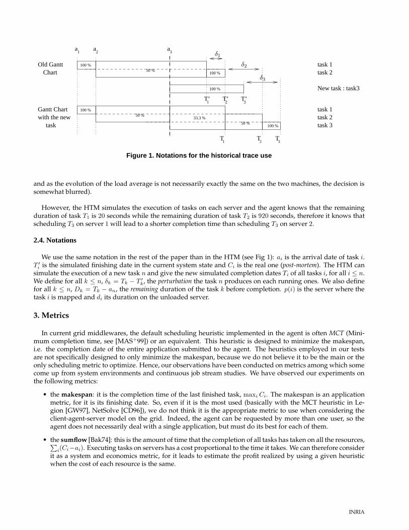
In order to make the estimations, the HTM performs a discrete simulation of the execution of each task. TheHTM can therefore build or update the Gantt chart for each server when a new incoming task is mapped as it ispresented in Figure 1. The agent disposes of the Gantt chart given on the top of the figure. Two tasks have beenscheduled on the server and a new one arrives at time t = a3. The agent simulates its execution. Therefore, thethree tasks share the processor capacity and each one receives 33.3% until time T1 where the first task finishes.Then, task 2 and task 3 receives 50% of the server CPU.
Using the HTM information leads to accurate prediction of the finishing time of the tasks assigned to a server,but the heuristics which have all those information can also consider the perturbation tasks have on each other, andconsequently envisage other metrics than the common makespan on which to score the servers. When assigninga new task, the HTM does not consider that the load of the server is constant to the one at the arrival date of thenew task all along its duration. Then, the information of the new or updated Gantt charts are used by the agentto schedule tasks more accurately to optimize the chosen metric.
The simulation of the distributed environment is done for each three parts of the tasks: input data transfer,computing phase and output data transfer.
Usefulness of the HTM Here follows an example that shows how the Historical Trace Manager can help intaking good scheduling decisions:
Let us suppose that the set of servers is made up of two identical servers (same network capabilities, same CPUpeak speed, same set of problems, etc.). At time 0, the client sends to these servers two tasks T1 and T2, whosedurations on each server is 100 and 1000 seconds respectively, with no input data. Let the agent schedule T1 onthe server 1 and T2 on the server 2 for example. At time 80, let a client request the agent to schedule a task T3
whose duration is 100 seconds.
Without the historical trace manager, the agent knows only that server 1 and server 2 have the same load andtherefore is not able to decide which is the best server to schedule T3 (in practice, as there are dynamic information
RR n° 5168
T’1
T’3
a3
T2
T1
T3
100 %50 %
50 %100 %
100 %
100 %
T’2
task 1task 2task 3
Gantt Chartwith the new
task
Old GanttChart
50 %100 %
33.3 %
a a1 2
task 1task 2
New task : task3
PSfrag replacements
δ1
δ2
δ3
Figure 1. Notations for the historical trace use
and as the evolution of the load average is not necessarily exactly the same on the two machines, the decision issomewhat blurred).
However, the HTM simulates the execution of tasks on each server and the agent knows that the remainingduration of task T1 is 20 seconds while the remaining duration of task T2 is 920 seconds, therefore it knows thatscheduling T3 on server 1 will lead to a shorter completion time than scheduling T3 on server 2.
2.4. Notations
We use the same notation in the rest of the paper than in the HTM (see Fig 1): ai is the arrival date of task i.T ′
i is the simulated finishing date in the current system state and Ci is the real one (post-mortem). The HTM cansimulate the execution of a new task n and give the new simulated completion dates Ti of all tasks i, for all i ≤ n.We define for all k ≤ n, δk = Tk − T ′
k, the perturbation the task n produces on each running ones. We also definefor all k ≤ n, Dk = Tk − an, the remaining duration of the task k before completion. p(i) is the server where thetask i is mapped and di its duration on the unloaded server.
3. Metrics
In current grid middlewares, the default scheduling heuristic implemented in the agent is often MCT (Mini-mum completion time, see [MAS+99]) or an equivalent. This heuristic is designed to minimize the makespan,i.e. the completion date of the entire application submitted to the agent. The heuristics employed in our testsare not specifically designed to only minimize the makespan, because we do not believe it to be the main or theonly scheduling metric to optimize. Hence, our observations have been conducted on metrics among which somecome up from system environments and continuous job stream studies. We have observed our experiments onthe following metrics:
• the makespan: it is the completion time of the last finished task, maxi Ci. The makespan is an applicationmetric, for it is its finishing date. So, even if it is the most used (basically with the MCT heuristic in Le-gion [GW97], NetSolve [CD96]), we do not think it is the appropriate metric to use when considering theclient-agent-server model on the grid. Indeed, the agent can be requested by more than one user, so theagent does not necessarily deal with a single application, but must do its best for each of them.
• the sumflow [Bak74]: this is the amount of time that the completion of all tasks has taken on all the resources,∑i(Ci−ai). Executing tasks on servers has a cost proportional to the time it takes. We can therefore consider
it as a system and economics metric, for it leads to estimate the profit realized by using a given heuristicwhen the cost of each resource is the same.
INRIA

• the maxstretch [BCM98]: we know by this value by what maximum factor, maxi ((Ci − ai)/di), a queryhas been slowed down relative to the time it takes on the same but unloaded server. A client can have anapproximation of the minimum time his task will take on a server, but a task can require much more timethan it would due to contention with previously allocated tasks and with hypothetical arriving ones. Thisvalue gives the worst case of slowdown for a task among all those submitted to the agent.
• the maxflow [BCM98]: this is the maximum time a task has spent in the system, maxi(Ci − ai). In a loadedsystem, a task will generally cost more than expected. This is even truer if it is allocated on a fast server(which is generally more solicited). This value can inform about high contention or about the use of theslowest servers in a high heterogeneous system.
• the meanflow which is also in our context where tasks are executed as soon as the input data is received themean response-time.
• the percentage of tasks that finish sooner: whereas this is not a metric, this value gives, in correlationto the previous metrics, a relevant idea of a quality of service given to each task when comparing twoheuristics. For instance, comparing the heuristics H1 with MCT (on the same set of tasks {t1 . . . tn} and sameenvironment), it is | {ti|Cti H1
< Cti MCT } | divided by n.
The user point of view is not that the last allocated task finishes the soonest (optimizing the makespan) butthat his own tasks (a subset of all client requests) finish as fast as possible. Therefore, if we can provide aheuristic where most of the tasks finish sooner than MCT’s without delaying too much other task completiondates (that can be verified with the sum-flow and the response-time for example), we can claim that thisheuristic, to the user point of view, outperforms MCT.
1 For each new task t2 For each server j that can resolve the new submitted problem3 Ask the HTM to compute the completion date of t, Tt, if t is executed on j4 Map task t to server j0 that minimizes Tt
5 Tell the HTM that task t is allocated to server j0
Figure 2. HMCT algorithm
1 For each new task t2 For each server j that can resolve the new submitted problem3 Ask the HTM to compute Pj =
∑i δi
4 If all Pj are equal5 map task to server j0 that minimizes Tt
6 Else Map task t to server j0 such as Pj0 = minj Pj
7 Tell the HTM that task t is allocated to server j0
Figure 3. MP algorithm
RR n° 5168
4. Proposed Heuristics
We have conducted several simulated experiments with the Simgrid API [Cas01]. Our investigations on severalheuristics are reported in [CJ02] where independent tasks have been submitted to the environment. Among them,some heuristics gave good results on most of the metrics observed here. Indeed, in the simulated experiments,these did generally not only optimize the makespan but also one or more other metrics. We only describe in thissection three of them that we have implemented and tested in real NetSolve environments: HMCT, MP and MSF.
When a new request arrives, the HTM simulates the execution of the task on each server. Our heuristics usethe HTM information, hence consider the perturbation that tasks induce on each other and compute the ‘best’server given an objective which is explained.
4.1. Historical Minimum Completion Time
HMCT is the MCT [MAS+99], Minimum Completion Time, algorithm relying on the HTM, in the time-sharemodel. When a new task arrives, the HTM simulates the mapping of the task on each server. Therefore, thescheduler has an estimation of the finishing date of this task on each server. The agent then allocates the task tothe server that minimizes its finishing date (see Fig. 2). Unlike MCT, which has been studied in the space-sharemodel, HMCT do not assume a constant behavior of the environment during the execution of the task to predictits finishing date (see Section 2.1). HMCT uses HTM estimations which are far more precise.
The goal of HMCT is the same as MCT’s: it expects to minimize the makespan of the application by minimizingthe completion date of incoming tasks.
The main drawback of this heuristic is that it tends to overload the fastest servers, which has two effects:unnecessarily delay task completion dates and servers may collapse, mainly due to a lack of memory or to theincapability to handle the too high throughput of requests.
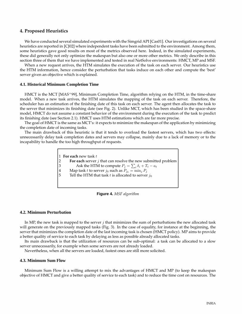
1 For each new task t2 For each server j that can resolve the new submitted problem3 Ask the HTM to compute Pj =
∑i δi + Tt − at
4 Map task t to server j0 such as Pj0 = minj Pj
5 Tell the HTM that task t is allocated to server j0
Figure 4. MSF algorithm
4.2. Minimum Perturbation
In MP, the new task is mapped to the server j that minimizes the sum of perturbations the new allocated taskwill generate on the previously mapped tasks (Fig. 3). In the case of equality, for instance at the beginning, theserver that minimizes the completion date of the last incoming task is chosen (HMCT policy). MP aims to providea better quality of service to each task by delaying as less as possible already allocated tasks.
Its main drawback is that the utilization of resources can be sub-optimal: a task can be allocated to a slowserver unnecessarily, for example when some servers are not already loaded.
Nevertheless, when all the servers are loaded, fastest ones are still more solicited.
4.3. Minimum Sum Flow
Minimum Sum Flow is a willing attempt to mix the advantages of HMCT and MP (to keep the makespanobjective of HMCT and give a better quality of service to each task) and to reduce the time cost on resources. The
INRIA

Scenario Application(s) Independent Tasks Experiment
nbclients width x depth nbtasks µ (sec) nbseeds x nbrun total nbtasks(a) 500 independent dgemm tasks - - 500 20 and 15 4 x 3 500(b) 500 independent tasks - - 500 20 and 15 3 x 3 , 3 x 5 500(c) 1D-mesh 10 1x50 - - 4 x 6 500(d) 1D-mesh 10 1x variable - - 4 x 6 500(e) 1D-mesh + 250 independent tasks 5 1x50 250 20 4 x 6 500(f) stencil (task 1) 1 10x50 - - 1 x 6 500(g) stencil (task 3) 1 10x50 - - 1 x 6 500(h) stencil + 174 independent tasks 1 10x25 174 28 2 x 3 424(i) stencil + 86 independent tasks 1 10x25 86 40 4 x 6 336(j) stencil + 86 independent tasks 1 5x25 86 25 4 x 6 211
Table 2. Scenarios, modalities and number of experiments
heuristic uses the HTM to compute the sum of the whole flow when assigning the last task to each server. Hence,the heuristic returns the identity of server j0 that minimizes the system sum flow, e.g.
minj
(
i=n∑
k 6=j,i=1
(T ′i,k − ai,k) +
i=n+1∑
i=1
(Ti,j − ai,j))
But as the difference between two values is only due to perturbations and to the new simulated task duration,the heuristic only needs to compute
∑t−1i=1 δi + Tt − at for each server j, that is to say the perturbation of the last
task on the server plus the HTM estimated length of the new task (Fig. 4). This heuristic is the same then MTI(Minimize Total Interference) proposed by Weissman in [Wei96].
5. Experiments
We have conducted simulation experiments to test several heuristics on the submission of independent tasksto an agent. Results are related in [CJ02].
A perfect modelling of a realistic environment including monitors is hard: for example, load information givenby censors and the frequency of the communications must be simplified (we work in a shared CPU context andscheduling decisions rely on the accuracy of the information given by the censors which, for example, return thenumber of tasks in place of the result of the ‘uptime’command). The objective of this work is to evaluate someof them in a real scale. Moreover, we also want to test them in experiments involving applications showing taskdependences. Hence, we have implemented the HTM and the three heuristics described in the previous section,HMCT, MP and MSF, that were a priori able to give good results in a real NetSolve platform. We have performedseveral experiments with different kind of applications.
We have compared our heuristics against an implementation of MCT (section 4.1, [MAS+99]), the schedulingheuristic used in NetSolve. The implementation in NetSolve of this heuristic benefits of some load correctionmechanisms: when the load of a server variates more than a given value, the server sends a load report to theagent, in the limit of one message per 60 seconds. Moreover, a mechanism adds a value to the chosen server lastrecorded load in the agent to take note of the affectation for further scheduling. Finally, the agent is informed ofthe finishing of a task and corrects the recorded load accordingly, waiting for a censor load report.
We firstly describe the application models, the different kind of tasks that compose a submitted application andthe modalities of the experiments. Then, we present in the corresponding subsection several sets of experiments,which we will refer next to scenarios, given in Table 2 (this table will be fully detailed in the next section).
RR n° 5168
5.1. Application Models, Task Types and Experiments Modalities
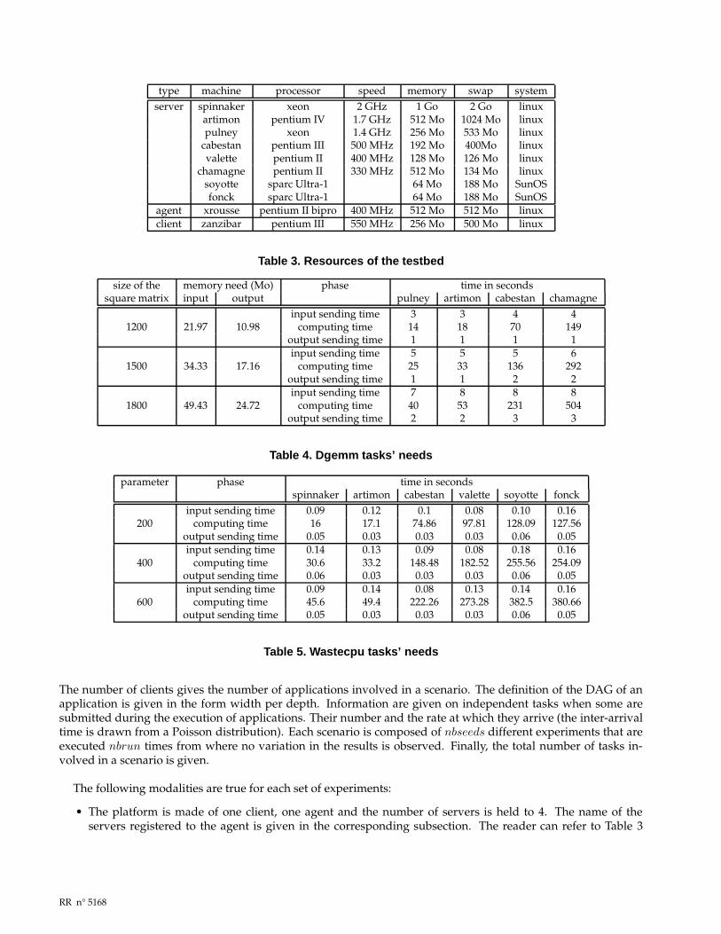
The experiments presented later are performed on a NetSolve environment composed of one client, one agentand four servers. The resources, given in Table 3, are distributed in the research center. They are interconnectedwith the research center network. Then, if servers are dedicated to the environment, the network is not. The setof servers composing the environment is given in the corresponding section.
A scenario involves one kind of task, which can be of the two following: dgemm or wastecpu. A dgemm is amatrix multiplication of the BLAS library. It needs more or less memory depending on the sizes of the matricesthat we generate randomly. Because of the heterogeneity of the NetSolve platform, we had troubles with Net-Solve using MCT. Indeed, servers collapsed as it is explained further. Hence, we have designed a CPU intensivetask which requires no memory that we have called wastecpu.
Given a kind of task, we use three different input data, conducting to three different durations. A task has auniform probability to be of each duration. The need of each task has been benchmarked, and the values has beenmade available directly in the code of NetSolve. Therefore, the HTM for our scheduling heuristics and NetSolveMCT use these values (Tables 4 and 5).
Dgemm tasks are multiplication of matrices of size 1200, 1500 or 1800. Parameters given to the wastecpu tasksare 200, 400, 600. We give in the next subsections what kind of task is used, and we refer to the fastest task by type1 (matrix of size 1200 or parameter equal to 200), an to the slowest task by type 3 (matrix of size 1800 or parameter600).
The submission of an independent task set can be submissions by one client of all of the tasks or at least onerequest by several clients. Previous works use that class of application to evaluate their performances [BSB+99,MAS+99]. As we explain later, we cannot expect a high difference on the makespan performance with MCT onthat kind of submission.
Results on independent tasks submission experiments led us to envisage the submission of applications withprecedence relations. But, as far as we know, there is no real structural benchmark for a typical application modelsubmitted in the client-agent-server model. Therefore, we have chosen to use linear applications, e.g. 1D meshapplications (fig 5), and stencil applications (fig 6) as applications implying precedence relations.
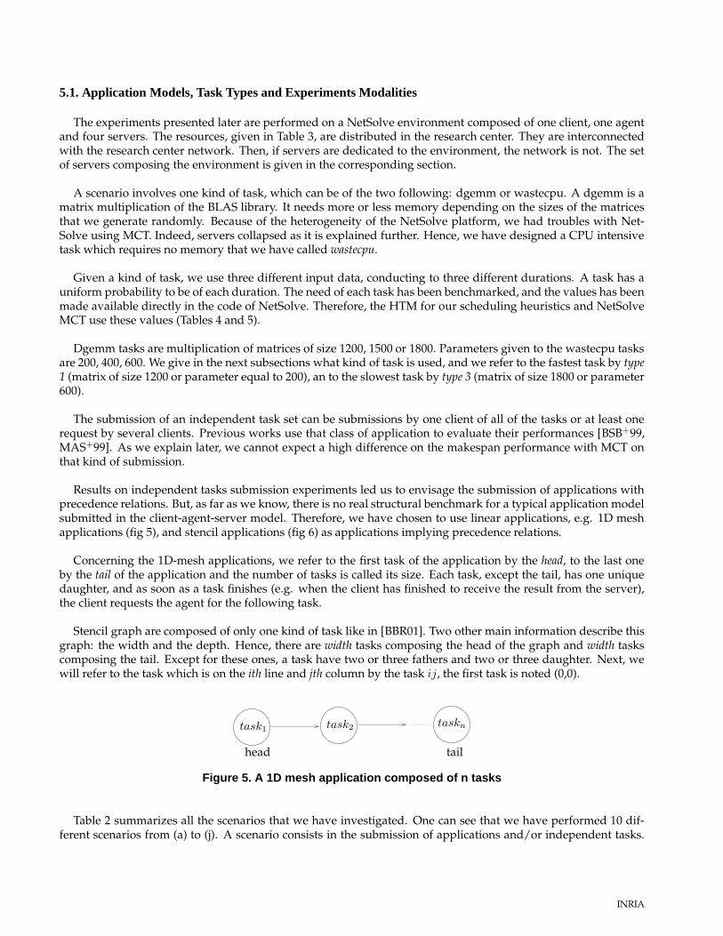
Concerning the 1D-mesh applications, we refer to the first task of the application by the head, to the last oneby the tail of the application and the number of tasks is called its size. Each task, except the tail, has one uniquedaughter, and as soon as a task finishes (e.g. when the client has finished to receive the result from the server),the client requests the agent for the following task.
Stencil graph are composed of only one kind of task like in [BBR01]. Two other main information describe thisgraph: the width and the depth. Hence, there are width tasks composing the head of the graph and width taskscomposing the tail. Except for these ones, a task have two or three fathers and two or three daughter. Next, wewill refer to the task which is on the ith line and jth column by the task ij, the first task is noted (0,0).PSfrag replacements
task1 task2 taskn
head tail
Figure 5. A 1D mesh application composed of n tasks
Table 2 summarizes all the scenarios that we have investigated. One can see that we have performed 10 dif-ferent scenarios from (a) to (j). A scenario consists in the submission of applications and/or independent tasks.
INRIA
type machine processor speed memory swap systemserver spinnaker xeon 2 GHz 1 Go 2 Go linux
artimon pentium IV 1.7 GHz 512 Mo 1024 Mo linuxpulney xeon 1.4 GHz 256 Mo 533 Mo linux
cabestan pentium III 500 MHz 192 Mo 400Mo linuxvalette pentium II 400 MHz 128 Mo 126 Mo linux
chamagne pentium II 330 MHz 512 Mo 134 Mo linuxsoyotte sparc Ultra-1 64 Mo 188 Mo SunOSfonck sparc Ultra-1 64 Mo 188 Mo SunOS
agent xrousse pentium II bipro 400 MHz 512 Mo 512 Mo linuxclient zanzibar pentium III 550 MHz 256 Mo 500 Mo linux
Table 3. Resources of the testbed
size of the memory need (Mo) phase time in secondssquare matrix input output pulney artimon cabestan chamagne
input sending time 3 3 4 41200 21.97 10.98 computing time 14 18 70 149
output sending time 1 1 1 1input sending time 5 5 5 6
1500 34.33 17.16 computing time 25 33 136 292output sending time 1 1 2 2input sending time 7 8 8 8
1800 49.43 24.72 computing time 40 53 231 504output sending time 2 2 3 3
Table 4. Dgemm tasks’ needs
parameter phase time in secondsspinnaker artimon cabestan valette soyotte fonck
input sending time 0.09 0.12 0.1 0.08 0.10 0.16200 computing time 16 17.1 74.86 97.81 128.09 127.56
output sending time 0.05 0.03 0.03 0.03 0.06 0.05input sending time 0.14 0.13 0.09 0.08 0.18 0.16
400 computing time 30.6 33.2 148.48 182.52 255.56 254.09output sending time 0.06 0.03 0.03 0.03 0.06 0.05input sending time 0.09 0.14 0.08 0.13 0.14 0.16
600 computing time 45.6 49.4 222.26 273.28 382.5 380.66output sending time 0.05 0.03 0.03 0.03 0.06 0.05
Table 5. Wastecpu tasks’ needs
The number of clients gives the number of applications involved in a scenario. The definition of the DAG of anapplication is given in the form width per depth. Information are given on independent tasks when some aresubmitted during the execution of applications. Their number and the rate at which they arrive (the inter-arrivaltime is drawn from a Poisson distribution). Each scenario is composed of nbseeds different experiments that areexecuted nbrun times from where no variation in the results is observed. Finally, the total number of tasks in-volved in a scenario is given.
The following modalities are true for each set of experiments:
• The platform is made of one client, one agent and the number of servers is held to 4. The name of theservers registered to the agent is given in the corresponding subsection. The reader can refer to Table 3
RR n° 5168

PSfrag replacements
task0 task1 task2 task3 task4
task10 task11
task20 taskij
Figure 6. 5x4 stencil task graph
to have further information on the platform resources. We call heterogeneity coefficient of the platform, themaximum on all servers and on all tasks of the division of the maximum computing need by the minimumcomputing need for the same task, e.g. maxtaski
maxservers di,s
minservers di,s;
• Only one kind of task (dgemm or wastecpu) is used to generate all the submitted applications in a scenario.Moreover, the same experiment has been carried out several times (equal to nbrun given in Table 2). This isreferred to as a run. Results are means on these runs ;
• There is 3 different possible sizes when a task of a given type is drawn. Then, one can generate 3n differentapplications composed of n tasks ;
• We note that in each experiment of each scenario, a scheduling decision cost is negligible compared to theduration of the shortest task (less than 0.1 second) for all the proposed heuristics.
5.2. Scenarios (a) and (b): Submission of 500 Independent Tasks
We present two kind of submissions with scenario (a) and (b): the first scenario is composed of dgemm tasksand the second is made of wastecpu tasks. As we consider in this paper three possible inputs, one can generate3500 different sets of independent tasks for one experiment in each scenario. Given a generated set of tasks, thedifference between two arrival dates is drawn from a Poisson distribution with a mean of µ = 20 seconds andµ = 15 seconds.
In the following, we describe more precisely the two scenarios then we explain the results.
5.2.1 Scenario (a): Dgemm Independent Tasks Submission
In the first set of experiments, the tasks are multiplications of square matrix (dgemm) of size 1200, 1500 and1800 leading to different time and memory cost (Table 4). The platform, described next, has an heterogeneouscoefficient equal to 504/40 = 12.6. For all the experiments, the testbed is composed of:
• client: zanzibar ;
• agent: xrousse ;
INRIA

NetSolve’s MCT HMCT MP MSFnumber of
completed tasks 500 500 500 500makespan 9906 9908 10162 9905sumflow 25922 19934 26383 19702maxflow 230 103 517 97
maxstretch 12.8 5.8 3.7 5.3percentage of
tasks that finish - 65% 66% 65%sooner than withNetSolve’s MCT
Table 6. Scenario (a): results in seconds for µ = 20 sec for dgemm Tasks
NetSolve’s MCT HMCT MP MSFnumber of
completed tasks 495 358 500 500makespan 7880 5600 7648 7626sumflow 89254 25092 34677 31375maxflow 1780 500 720 250
maxstretch 99 27.8 6.3 11.3percentage of
tasks that finish - <85%> 84% 87%sooner than withNetSolve’s MCT
Table 7. Scenario (a): results in seconds for µ = 15 sec for dgemm Tasks
• servers: chamagne ; pulney ; cabestan ; artimon.
Results on the makespan, the sumflow for µ = 20 seconds are given in Table 6 summarizes mean results forµ = 20 seconds on the number of completed tasks, the makespan, the sumflow, the maxflow, the maxstretch andthe percentage of tasks that finish sooner than if scheduled with MCT.
In Table 7, where µ = 15 and built the same way than the previous one, values for MCT and HMCT results arethose obtained from the run when the number of completed tasks was the maximum. Indeed, for µ = 15, MCTand HMCT are not able to handle the throughput of tasks. HMCT and MCT overload the fastest servers thatcannot accept any more jobs because they run out of memory. However, the NetSolve MCT has fault tolerancemechanisms that permit to schedule almost all tasks on some runs. For µ = 20, this phenomenon does not occurbecause the arrival rate lets faster servers complete more tasks before a new request.
One should note that for µ = 15 seconds, the NetSolve MCT gives very high values, and the highest for all theobserved metrics, showing lesser performances. There is a huge time and space contention on the fastest servers.This is confirmed, for MCT and for HMCT, by the load average sent to the agent (more than 12 on pulney).Consequently, some servers collapsed during the experiment.
Even when there is low contention, e.g. when µ = 20 seconds, one can see from the results that using anheuristic that uses HTM information leads to better performances than MCT benefiting from load correctionmechanisms. From these results, MSF is the best heuristic: it achieves the best performances regardless the metricand the rate of incoming submissions.
5.2.2 Scenario (b): Wastecpu Independent Tasks Submission
We use wastecpu tasks to prevent memory problems that we do not yet handle. The goal is to replace the multi-plication tasks, so its computation costs, dependent on the parameters, are similar to the multiplication tasks. Awastecpu task can have the parameter 200, 400 or 600 which determines the time it costs (Table 5).
RR n° 5168

Two platform have been used. We give next the experimentations and the results obtained for each of them.For the both of them, we can remark with relief that two runs of the same experiment give slightly the sameresults. This explains the small number of experiments undertaken. Moreover, for this scenario, all tasks of eachset have been submitted, accepted and computed by all of the five heuristics we have tested.
Platform 1 The heterogenous coefficient (the maximum computing cost divided by the minimum for the sametask) of the platform described next is 97/16 = 6. The experimental testbed for this set of experiments is made upof:
• client: zanzibar ;
• agent: xrousse ;
• servers: valette ; spinnaker ; cabestan ; artimon.
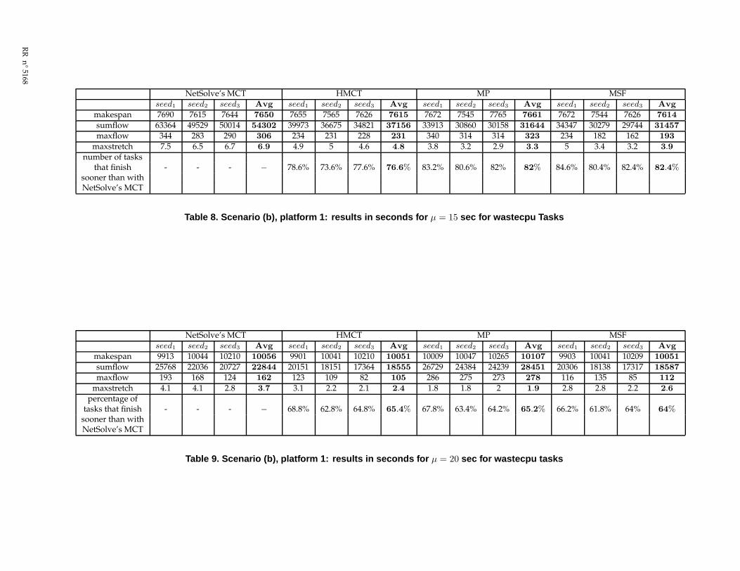
We generated three different sets of tasks, submitted at two different arrival rates. Results for µ = 20 seconds,given in Table 9, are obtained from 2 executions of the same metatask scheduled by each of the four tested heuris-tics. At this rate, the experiment finishes after about 10, 000 seconds. In Table 8, for µ = 15 seconds, values arethe mean of 4 executions for the NetSolve MCT and 3 for the three others. At this rate, the experiment needsabout 7, 700 seconds to complete. For a set of independent tasks scheduled according to a given heuristic, thepercentage of tasks that finish sooner is the mean of the values obtained from the comparison between each runfor this heuristic and each run for NetSolve (hence obtained from a comparison in ‘cross product’). Finally, we givein the column ‘Avg’ the mean on the observed metric of the values obtained for each run and each set.
HMCT and MSF outperform MCT regardless the rate and the observed metric. If they give slightly the sameresults for µ = 20, MSF even outperforms HMCT when µ = 15 seconds. On the opposite, MP shows performancegains only for µ = 15 seconds. Our heuristics are specifically designed for environments with contention: gainsincrease with it.
INRIA
NetSolve’s MCT HMCT MP MSFseed1 seed2 seed3 Avg seed1 seed2 seed3 Avg seed1 seed2 seed3 Avg seed1 seed2 seed3 Avg
makespan 7690 7615 7644 7650 7655 7565 7626 7615 7672 7545 7765 7661 7672 7544 7626 7614
sumflow 63364 49529 50014 54302 39973 36675 34821 37156 33913 30860 30158 31644 34347 30279 29744 31457
maxflow 344 283 290 306 234 231 228 231 340 314 314 323 234 182 162 193
maxstretch 7.5 6.5 6.7 6.9 4.9 5 4.6 4.8 3.8 3.2 2.9 3.3 5 3.4 3.2 3.9
number of tasksthat finish - - - − 78.6% 73.6% 77.6% 76.6% 83.2% 80.6% 82% 82% 84.6% 80.4% 82.4% 82.4%
sooner than withNetSolve’s MCT
Table 8. Scenario (b), platform 1: results in seconds for µ = 15 sec for wastecpu Tasks
NetSolve’s MCT HMCT MP MSFseed1 seed2 seed3 Avg seed1 seed2 seed3 Avg seed1 seed2 seed3 Avg seed1 seed2 seed3 Avg
makespan 9913 10044 10210 10056 9901 10041 10210 10051 10009 10047 10265 10107 9903 10041 10209 10051
sumflow 25768 22036 20727 22844 20151 18151 17364 18555 26729 24384 24239 28451 20306 18138 17317 18587
maxflow 193 168 124 162 123 109 82 105 286 275 273 278 116 135 85 112
maxstretch 4.1 4.1 2.8 3.7 3.1 2.2 2.1 2.4 1.8 1.8 2 1.9 2.8 2.8 2.2 2.6
percentage oftasks that finish - - - − 68.8% 62.8% 64.8% 65.4% 67.8% 63.4% 64.2% 65.2% 66.2% 61.8% 64% 64%
sooner than withNetSolve’s MCT
Table 9. Scenario (b), platform 1: results in seconds for µ = 20 sec for wastecpu tasks
RR
n°5168

Platform 2 The heterogeneous coefficient of the second platform is slightly superior to the previous and equalto 8.9. The following resources composed the environment:
• client: zanzibar ;
• agent: xrousse ;
• servers: spinnaker, artimon, soyotte, fonck.
Three different seeds have been used to instantiate Scenario (b), and the resulting experiments have been sub-mitted at three different rates: 20, 17 and 15 seconds. For µ = 17 and µ = 20 seconds, each experiment has beensubmitted 3 times conducting to 9 submissions per rate and per heuristic for this scenario. For µ = 15 seconds,each experiment has been submitted 6 times then 15 submissions have been performed on the platform for thisrate and for each heuristic. Tables presenting the results for µ = 20 are detailed next. Tables for µ = 17 and µ = 15are built the same way.
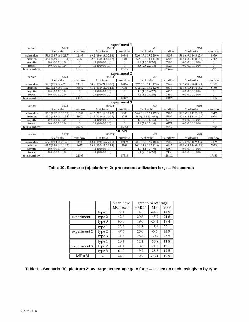
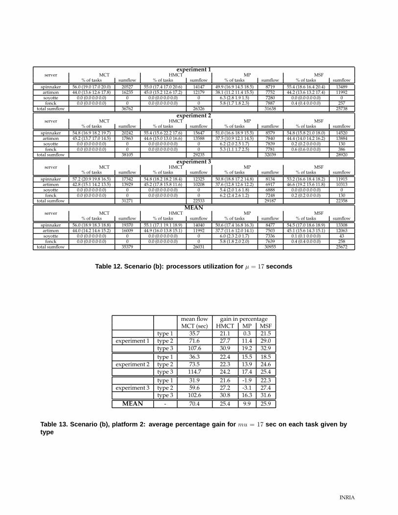
Results for the inter-arrival µ = 20 seconds are given in Tables 10, 11, 16. We describe in Table 10 the utilizationof each server by each heuristic during each experiment: given an experiment, each percentage of allocated taskson the 500 of the experiment (the corresponding part of each task type is precised in parenthesis) per server isgiven. The sumflow per server as well as the total sumflow that the experiment costs is also given.
Table 11 gives the mean flow recorded during the submission of the experiment scheduled by MCT and theaverage gain for each task type over MCT if the same experiment is scheduled by a given heuristic.
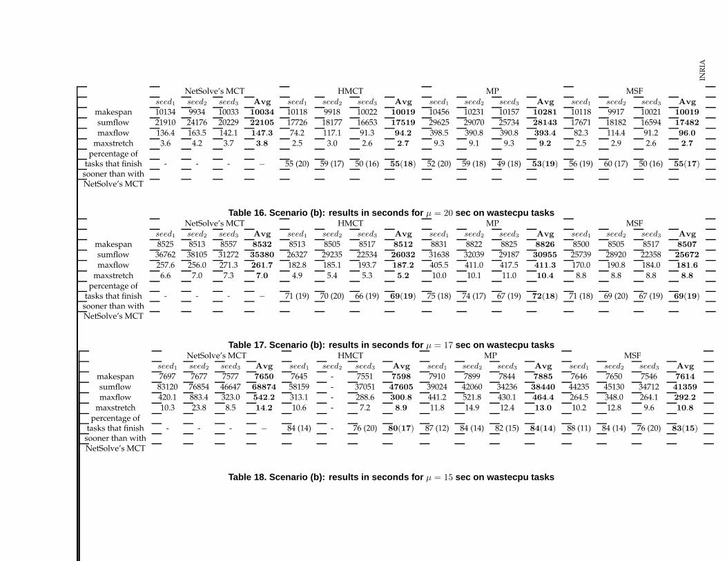
Table 16 summarizes many information: for each heuristic and each seed, mean results on the makespan, thesumflow, the maxflow, the maxstretch and the number of tasks finishing sooner than if scheduled by MCT aregiven.
Like for the previous platform, for each seed and each heuristic (naturally except MCT) the percentage of tasksthat finish sooner is the average percentage obtained from the comparison of terminaison dates between each runfor this heuristic and each run for NetSolve (hence from a comparison in ‘cross product’). A task is considered‘finishing sooner’ if the terminaison dates differ from at least 2 seconds between MCT and the other heuristic.Thus, we give in parenthesis the percentage of tasks that finish sooner with MCT than with the given heuristic:because there exists tasks that finish in a range of 2 seconds between a run with MCT and with another heuristic,the sum of the percentage of tasks that finish sooner with our heuristic and the percentage of tasks that finishsooner with MCT differs from 100. Finally the column ‘Avg’ contains the mean on the observed metric of thevalues for each run and each seed.
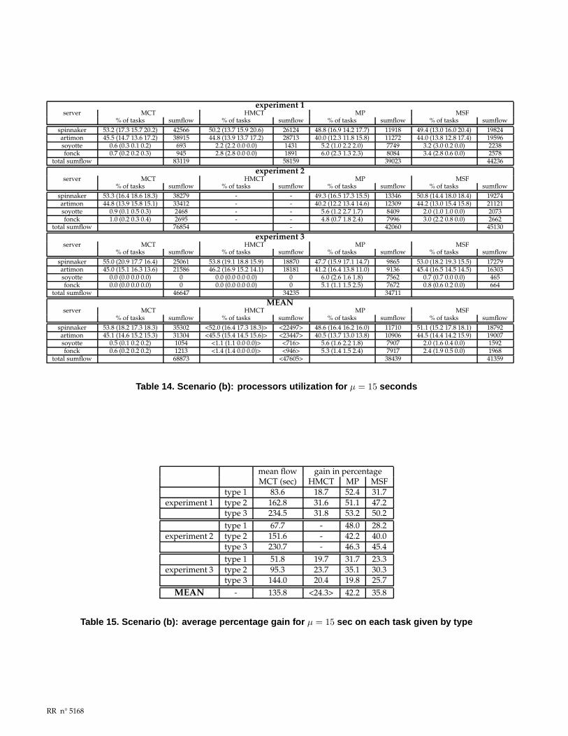
The same experiments have been conducted with µ = 17 and µ = 15 seconds and we present the results re-spectively in Tables 12, 13, 17 and in Tables 14, 15, 18.
With Tables 10, 12 and 14, one can see the evolution of the processor utilization in function of the heuristic.Regardless the heuristic, the percentage of tasks scheduled on spinnaker decreases slightly: all types of tasks areconcerned in the same manner. This benefits to the slower servers: only to artimon for HMCT, but MP and MSFgive also more jobs to fonck and soyotte.
If HMCT and MSF have the same behavior and outperform both MP and MCT for µ = 20 and µ = 17, MPachieves to reduce the total sumflow progression and outperfom all the others for µ15 seconds.
Table 11 confirms that for slow rate, MP achieve sub-optimal scheduling. The average gain over MCT is neg-ative: each task scheduled by MCT is 28% shorter than with MP. On the opposite, at this rate, HMCT and MSFshow nearly the same positive results: their scheduling leads to gain 20% on each task flow. Due to perturbations,when the rate increases to µ = 17 seconds, the average flow grows to 160% bigger with MCT. All of our heuristicsoutperfom MCT, HMCT and MSF maximising the gains for each task, allowing them to be 26% shorter. When therate is high (µ = 15), MP achieves the best gains with an average flow 42% shorter than for MCT.
INRIA
experiment 1server MCT HMCT MP MSF
% of tasks sumflow % of tasks sumflow % of tasks sumflow % of tasks sumflowspinnaker 56.9 (18.7 16.5 21.7) 12463 60.2 (19.6 18.0 22.6) 10344 52.6 (17.4 15.2 20.0) 8103 58.6 (19.4 16.8 22.4) 9959artimon 43.1 (13.9 13.1 16.1) 9447 39.8 (13.0 11.6 15.2) 7381 35.2 (10.8 10.4 14.0) 6307 41.4 (13.2 12.8 15.4) 7712soyotte 0.0 (0.0 0.0 0.0) 0 0.0 (0.0 0.0 0.0) 0 5.4 (1.6 1.8 2.0) 7185 0.0 (0.0 0.0 0.0) 0fonck 0.0 (0.0 0.0 0.0) 0 0.0 (0.0 0.0 0.0) 0 6.8 (2.8 2.2 1.8) 8029 0.0 (0.0 0.0 0.0) 0
total sumflow 21910 17725 29624 17671experiment 2
server MCT HMCT MP MSF% of tasks sumflow % of tasks sumflow % of tasks sumflow % of tasks sumflow
spinnaker 57.3 (17.9 19.4 20.0) 13515 58.8 (17.6 21.2 20.0) 10196 52.2 (15.8 19.0 17.4) 7949 58.6 (18.8 20.8 19.0) 10002artimon 42.7 (12.7 15.8 14.2) 10662 41.2 (13.0 14.0 14.2) 7981 37.2 (12.0 13.2 12.0) 6319 41.4 (11.8 14.4 15.2) 8180soyotte 0.0 (0.0 0.0 0.0) 0 0.0 (0.0 0.0 0.0) 0 4.8 (1.0 1.6 2.2) 6916 0.0 (0.0 0.0 0.0) 0fonck 0.0 (0.0 0.0 0.0) 0 0.0 (0.0 0.0 0.0) 0 5.8 (1.8 1.4 2.6) 7885 0.0 (0.0 0.0 0.0) 0
total sumflow 24177 18177 29069 18182experiment 3
server MCT HMCT MP MSF% of tasks sumflow % of tasks sumflow % of tasks sumflow % of tasks sumflow
spinnaker 57.8 (21.7 19.9 16.2) 11307 61.3 (22.1 19.9 19.3) 9908 54.4 (19.8 17.4 17.2) 7907 59.6 (21.2 19.2 19.2) 9617artimon 42.2 (14.3 14.1 13.8) 8922 38.7 (13.9 14.1 10.7) 6745 36.0 (12.6 13.8 9.6) 5809 40.4 (14.8 14.8 10.8) 6978soyotte 0.0 (0.0 0.0 0.0) 0 0.0 (0.0 0.0 0.0) 0 4.0 (0.8 1.6 1.6) 5640 0.0 (0.0 0.0 0.0) 0fonck 0.0 (0.0 0.0 0.0) 0 0.0 (0.0 0.0 0.0) 0 5.6 (2.8 1.2 1.6) 6377 0.0 (0.0 0.0 0.0) 0
total sumflow 20229 16653 25733 16595MEAN
server MCT HMCT MP MSF% of tasks sumflow % of tasks sumflow % of tasks sumflow % of tasks sumflow
spinnaker 57.3 (19.4 18.6 19.3) 12428 60.1 (19.8 19.7 20.6) 10149 53.1 (17.7 17.2 18.2) 7986 58.9 (19.8 18.9 20.2) 9859artimon 42.7 (13.6 14.3 14.7) 9677 39.9 (13.3 13.2 13.4) 7369 36.1 (11.8 12.5 11.9) 6145 41.1 (13.3 14.0 13.8) 7623soyotte 0.0 (0.0 0.0 0.0) 0 0.0 (0.0 0.0 0.0) 0 4.7 (1.1 1.7 1.9) 6580 0.0 (0.0 0.0 0.0) 0fonck 0.0 (0.0 0.0 0.0) 0 0.0 (0.0 0.0 0.0) 0 6.1 (2.5 1.6 2.0) 7430 0.0 (0.0 0.0 0.0) 0
total sumflow 22105 17518 28142 17483
Table 10. Scenario (b), platform 2: processors utilization for µ = 20 seconds
mean flow gain in percentageMCT (sec) HMCT MP MSF
type 1 22.1 14.5 -44.9 14.9experiment 1 type 2 42.6 20.8 -45.2 21.8
type 3 63.5 19.6 -27.1 19.4type 1 23.2 21.5 -15.6 22.1
experiment 2 type 2 47.5 25.0 -6.6 24.9type 3 71.7 25.6 -30.9 25.5type 1 20.3 12.1 -35.8 11.8
experiment 3 type 2 41.1 18.6 -21.2 19.1type 3 64.0 19.2 -28.3 19.5
MEAN - 44.0 19.7 -28.4 19.9
Table 11. Scenario (b), platform 2: average percentage gain for µ = 20 sec on each task given by type
RR n° 5168
experiment 1server MCT HMCT MP MSF
% of tasks sumflow % of tasks sumflow % of tasks sumflow % of tasks sumflowspinnaker 56.0 (19.0 17.0 20.0) 20527 55.0 (17.4 17.0 20.6) 14147 49.9 (16.9 14.5 18.5) 8719 55.4 (18.6 16.4 20.4) 13489artimon 44.0 (13.6 12.6 17.8) 16235 45.0 (15.2 12.6 17.2) 12179 38.1 (11.2 11.4 15.5) 7752 44.2 (13.6 13.2 17.4) 11992soyotte 0.0 (0.0 0.0 0.0) 0 0.0 (0.0 0.0 0.0) 0 6.3 (2.8 1.9 1.5) 7280 0.0 (0.0 0.0 0.0) 0fonck 0.0 (0.0 0.0 0.0) 0 0.0 (0.0 0.0 0.0) 0 5.8 (1.7 1.8 2.3) 7887 0.4 (0.4 0.0 0.0) 257
total sumflow 36762 26326 31638 25738experiment 2
server MCT HMCT MP MSF% of tasks sumflow % of tasks sumflow % of tasks sumflow % of tasks sumflow
spinnaker 54.8 (16.9 18.2 19.7) 20242 55.4 (15.6 22.2 17.6) 15647 51.0 (16.6 18.9 15.5) 8579 54.8 (15.8 21.0 18.0) 14520artimon 45.2 (13.7 17.0 14.5) 17863 44.6 (15.0 13.0 16.6) 13588 37.5 (10.9 12.1 14.5) 7840 44.4 (14.0 14.2 16.2) 13884soyotte 0.0 (0.0 0.0 0.0) 0 0.0 (0.0 0.0 0.0) 0 6.2 (2.0 2.5 1.7) 7839 0.2 (0.2 0.0 0.0) 130fonck 0.0 (0.0 0.0 0.0) 0 0.0 (0.0 0.0 0.0) 0 5.3 (1.1 1.7 2.5) 7781 0.6 (0.6 0.0 0.0) 386
total sumflow 38105 29235 32039 28920
experiment 3server MCT HMCT MP MSF
% of tasks sumflow % of tasks sumflow % of tasks sumflow % of tasks sumflowspinnaker 57.2 (20.9 19.8 16.5) 17342 54.8 (18.2 18.2 18.4) 12325 50.8 (18.8 17.2 14.8) 8134 53.2 (16.6 18.4 18.2) 11915artimon 42.8 (15.1 14.2 13.5) 13929 45.2 (17.8 15.8 11.6) 10208 37.6 (12.8 12.6 12.2) 6917 46.6 (19.2 15.6 11.8) 10313soyotte 0.0 (0.0 0.0 0.0) 0 0.0 (0.0 0.0 0.0) 0 5.4 (2.0 1.6 1.8) 6888 0.0 (0.0 0.0 0.0) 0fonck 0.0 (0.0 0.0 0.0) 0 0.0 (0.0 0.0 0.0) 0 6.2 (2.4 2.6 1.2) 7248 0.2 (0.2 0.0 0.0) 130
total sumflow 31271 22533 29187 22358MEAN
server MCT HMCT MP MSF% of tasks sumflow % of tasks sumflow % of tasks sumflow % of tasks sumflow
spinnaker 56.0 (18.9 18.3 18.8) 19370 55.1 (17.1 19.1 18.9) 14040 50.6 (17.4 16.8 16.3) 8477 54.5 (17.0 18.6 18.9) 13308artimon 44.0 (14.2 14.6 15.2) 16009 44.9 (16.0 13.8 15.1) 11992 37.7 (11.6 12.0 14.1) 7503 45.1 (15.6 14.3 15.1) 12063soyotte 0.0 (0.0 0.0 0.0) 0 0.0 (0.0 0.0 0.0) 0 6.0 (2.3 2.0 1.7) 7336 0.1 (0.1 0.0 0.0) 43fonck 0.0 (0.0 0.0 0.0) 0 0.0 (0.0 0.0 0.0) 0 5.8 (1.8 2.0 2.0) 7639 0.4 (0.4 0.0 0.0) 258
total sumflow 35379 26031 30955 25672
Table 12. Scenario (b): processors utilization for µ = 17 seconds
mean flow gain in percentageMCT (sec) HMCT MP MSF
type 1 35.7 21.1 0.3 21.5experiment 1 type 2 71.6 27.7 11.4 29.0
type 3 107.6 30.9 19.2 32.9type 1 36.3 22.4 15.5 18.5
experiment 2 type 2 73.5 22.3 13.9 24.6type 3 114.7 24.2 17.4 25.4type 1 31.9 21.6 -1.9 22.3
experiment 3 type 2 59.6 27.2 -3.1 27.4type 3 102.6 30.8 16.3 31.6
MEAN - 70.4 25.4 9.9 25.9
Table 13. Scenario (b), platform 2: average percentage gain for mu = 17 sec on each task given bytype
INRIA
experiment 1server MCT HMCT MP MSF
% of tasks sumflow % of tasks sumflow % of tasks sumflow % of tasks sumflowspinnaker 53.2 (17.3 15.7 20.2) 42566 50.2 (13.7 15.9 20.6) 26124 48.8 (16.9 14.2 17.7) 11918 49.4 (13.0 16.0 20.4) 19824artimon 45.5 (14.7 13.6 17.2) 38915 44.8 (13.9 13.7 17.2) 28713 40.0 (12.3 11.8 15.8) 11272 44.0 (13.8 12.8 17.4) 19596soyotte 0.6 (0.3 0.1 0.2) 693 2.2 (2.2 0.0 0.0) 1431 5.2 (1.0 2.2 2.0) 7749 3.2 (3.0 0.2 0.0) 2238fonck 0.7 (0.2 0.2 0.3) 945 2.8 (2.8 0.0 0.0) 1891 6.0 (2.3 1.3 2.3) 8084 3.4 (2.8 0.6 0.0) 2578
total sumflow 83119 58159 39023 44236experiment 2
server MCT HMCT MP MSF% of tasks sumflow % of tasks sumflow % of tasks sumflow % of tasks sumflow
spinnaker 53.3 (16.4 18.6 18.3) 38279 - - 49.3 (16.5 17.3 15.5) 13346 50.8 (14.4 18.0 18.4) 19274artimon 44.8 (13.9 15.8 15.1) 33412 - - 40.2 (12.2 13.4 14.6) 12309 44.2 (13.0 15.4 15.8) 21121soyotte 0.9 (0.1 0.5 0.3) 2468 - - 5.6 (1.2 2.7 1.7) 8409 2.0 (1.0 1.0 0.0) 2073fonck 1.0 (0.2 0.3 0.4) 2695 - - 4.8 (0.7 1.8 2.4) 7996 3.0 (2.2 0.8 0.0) 2662
total sumflow 76854 - 42060 45130experiment 3
server MCT HMCT MP MSF% of tasks sumflow % of tasks sumflow % of tasks sumflow % of tasks sumflow
spinnaker 55.0 (20.9 17.7 16.4) 25061 53.8 (19.1 18.8 15.9) 18870 47.7 (15.9 17.1 14.7) 9865 53.0 (18.2 19.3 15.5) 17279artimon 45.0 (15.1 16.3 13.6) 21586 46.2 (16.9 15.2 14.1) 18181 41.2 (16.4 13.8 11.0) 9136 45.4 (16.5 14.5 14.5) 16303soyotte 0.0 (0.0 0.0 0.0) 0 0.0 (0.0 0.0 0.0) 0 6.0 (2.6 1.6 1.8) 7562 0.7 (0.7 0.0 0.0) 465fonck 0.0 (0.0 0.0 0.0) 0 0.0 (0.0 0.0 0.0) 0 5.1 (1.1 1.5 2.5) 7672 0.8 (0.6 0.2 0.0) 664
total sumflow 46647 34235 34711MEAN
server MCT HMCT MP MSF% of tasks sumflow % of tasks sumflow % of tasks sumflow % of tasks sumflow
spinnaker 53.8 (18.2 17.3 18.3) 35302 <52.0 (16.4 17.3 18.3)> <22497> 48.6 (16.4 16.2 16.0) 11710 51.1 (15.2 17.8 18.1) 18792artimon 45.1 (14.6 15.2 15.3) 31304 <45.5 (15.4 14.5 15.6)> <23447> 40.5 (13.7 13.0 13.8) 10906 44.5 (14.4 14.2 15.9) 19007soyotte 0.5 (0.1 0.2 0.2) 1054 <1.1 (1.1 0.0 0.0)> <716> 5.6 (1.6 2.2 1.8) 7907 2.0 (1.6 0.4 0.0) 1592fonck 0.6 (0.2 0.2 0.2) 1213 <1.4 (1.4 0.0 0.0)> <946> 5.3 (1.4 1.5 2.4) 7917 2.4 (1.9 0.5 0.0) 1968
total sumflow 68873 <47605> 38439 41359
Table 14. Scenario (b): processors utilization for µ = 15 seconds
mean flow gain in percentageMCT (sec) HMCT MP MSF
type 1 83.6 18.7 52.4 31.7experiment 1 type 2 162.8 31.6 51.1 47.2
type 3 234.5 31.8 53.2 50.2type 1 67.7 - 48.0 28.2
experiment 2 type 2 151.6 - 42.2 40.0type 3 230.7 - 46.3 45.4type 1 51.8 19.7 31.7 23.3
experiment 3 type 2 95.3 23.7 35.1 30.3type 3 144.0 20.4 19.8 25.7
MEAN - 135.8 <24.3> 42.2 35.8
Table 15. Scenario (b): average percentage gain for µ = 15 sec on each task given by type
RR n° 5168
NetSolve’s MCT HMCT MP MSFseed1 seed2 seed3 Avg seed1 seed2 seed3 Avg seed1 seed2 seed3 Avg seed1 seed2 seed3 Avg
makespan 10134 9934 10033 10034 10118 9918 10022 10019 10456 10231 10157 10281 10118 9917 10021 10019
sumflow 21910 24176 20229 22105 17726 18177 16653 17519 29625 29070 25734 28143 17671 18182 16594 17482
maxflow 136.4 163.5 142.1 147.3 74.2 117.1 91.3 94.2 398.5 390.8 390.8 393.4 82.3 114.4 91.2 96.0
maxstretch 3.6 4.2 3.7 3.8 2.5 3.0 2.6 2.7 9.3 9.1 9.3 9.2 2.5 2.9 2.6 2.7
percentage oftasks that finish - - - − 55 (20) 59 (17) 50 (16) 55(18) 52 (20) 59 (18) 49 (18) 53(19) 56 (19) 60 (17) 50 (16) 55(17)
sooner than withNetSolve’s MCT
Table 16. Scenario (b): results in seconds for µ = 20 sec on wastecpu tasksNetSolve’s MCT HMCT MP MSF
seed1 seed2 seed3 Avg seed1 seed2 seed3 Avg seed1 seed2 seed3 Avg seed1 seed2 seed3 Avg
makespan 8525 8513 8557 8532 8513 8505 8517 8512 8831 8822 8825 8826 8500 8505 8517 8507
sumflow 36762 38105 31272 35380 26327 29235 22534 26032 31638 32039 29187 30955 25739 28920 22358 25672
maxflow 257.6 256.0 271.3 261.7 182.8 185.1 193.7 187.2 405.5 411.0 417.5 411.3 170.0 190.8 184.0 181.6
maxstretch 6.6 7.0 7.3 7.0 4.9 5.4 5.3 5.2 10.0 10.1 11.0 10.4 8.8 8.8 8.8 8.8
percentage oftasks that finish - - - − 71 (19) 70 (20) 66 (19) 69(19) 75 (18) 74 (17) 67 (19) 72(18) 71 (18) 69 (20) 67 (19) 69(19)
sooner than withNetSolve’s MCT
Table 17. Scenario (b): results in seconds for µ = 17 sec on wastecpu tasksNetSolve’s MCT HMCT MP MSF
seed1 seed2 seed3 Avg seed1 seed2 seed3 Avg seed1 seed2 seed3 Avg seed1 seed2 seed3 Avg
makespan 7697 7677 7577 7650 7645 - 7551 7598 7910 7899 7844 7885 7646 7650 7546 7614
sumflow 83120 76854 46647 68874 58159 - 37051 47605 39024 42060 34236 38440 44235 45130 34712 41359
maxflow 420.1 883.4 323.0 542.2 313.1 - 288.6 300.8 441.2 521.8 430.1 464.4 264.5 348.0 264.1 292.2
maxstretch 10.3 23.8 8.5 14.2 10.6 - 7.2 8.9 11.8 14.9 12.4 13.0 10.2 12.8 9.6 10.8
percentage oftasks that finish - - - − 84 (14) - 76 (20) 80(17) 87 (12) 84 (14) 82 (15) 84(14) 88 (11) 84 (14) 76 (20) 83(15)
sooner than withNetSolve’s MCT
Table 18. Scenario (b): results in seconds for µ = 15 sec on wastecpu tasks
INR
IA
5.2.3 Results
We have considered in this subsection the scheduling of a set of independent tasks whose inter-submissions fol-low a Poisson distribution of parameter µ equal to 15, 17 or 20 seconds. Therefore, the makespan is stronglydependent on the latest task arrival. We cannot expect at the very outset a big difference between two heuristicson that metric especially at low rate [MAS+99], even in a CPU shared environment. That is verified by our tests.Nonetheless, heuristics do not have the same performances.
The overall results converge even if gains are a bit better on the experiments performed on Platform 2: at thesame rate, there is more contention as the heterogeneity increases. Thus our heuristics that are designed to takeinto account the contention behave even better.
One can note that MCT and HMCT tend to not use the slowest servers fonck and soyotte. Indeed, a task hasto finish sooner on soyotte than on spinnaker to be scheduled there: this implies sufficient perturbations to doso, i.e. that during the execution of the task on spinnaker a number of tasks superior to the heterogeneity co-efficient be running concurrently for HMCT as well as an sufficient load on artimon as well. This clearly limitsthe throughput of tasks and even make HMCT unable to handle the second experiment on the platform 2 whenµ = 15 seconds.
To see how useful the HTM is, we compare results on the same heuristic: MCT and HMCT (in fact, these arenot exactly the same due to NetSolve load correction mechanisms). We see in Table 9 that HMCT needs onemissing hour (4289 seconds) of computations for a set of independent tasks whose time cost is of less than threehours (µ = 20) for the same makespan. Its performances are greater as the rate increases: a gain of 4.8 hours ofcomputations for a duration of 2.1 hours, and there too, a better quality of service (Table 8).
Moreover, a better quality of service is offered regardless the rate: HMCT shows a gain in average responsetime in Tables 11, 13 and 15 but cases exist where it cannot handle the throughput of submissions. Results arealways better for HMCT, and gains increase with the rate (see Tables 16, 17 and 18).
In consequence, the use of the HTM definitely leads to better results for Scenario (a) and (b), where the set ofindependent tasks can be perceived as one client with many tasks or many clients with at least one tasks.
MP has a better load balance property than MCT and HMCT (Table 9 and 8). Hence, when µ is large (lowarrival rate), it loads slower servers because they are idle. Whereas, when µ is low, no servers are idle, thenMP, like HMCT and MSF, tends also to load the fastest ones. MP presents the highest maxflow. It seems logicalconsidering that:
• for µ = 20, as tasks on faster servers are not necessarily finished, slower servers are used. The MP maxflowcomes from the maximum cost of a task on the slowest server.
• for µ = 15, there is contention even on the slowest servers. A task that had already a higher duration thanif allocated to a faster server requires even more time.
Therefore at low rate, MP is sub-optimal, but is rather good at higher rates: less sumflow (even compared to MSF)and a high number of tasks that finish sooner than MCT.
MSF tries to optimize the sumflow, hence finds a good balance between minimizing the perturbation andminimizing the new task duration. Therefore, it gives good performances on the makespan, the sumflow, evenon the maxflow and the percentage of tasks that finish sooner than with MCT is always very high (nearly the samethan MP’s for µ = 15 !). While MSF is not explicitly designed to optimize the makespan as is MCT, it appears thatit always outperforms MCT, as well as HMCT and MP on most of the metrics. Considering that an agent cannotguess the rate of the requests it will have to process, MSF is the best because it gives the same performances thanHMCT at low rates and better performances than others at higher rates.
5.3. Scenario (c): Submission of 10 1D-mesh Applications, Each Composed of 50 Wastecpu Tasks
An experiment consists in the submission of 10 applications composed of 50 wastecpu tasks each. An applica-tion is a 1D-mesh application (section 5.1), hence, when a client has received the result of its task, he immediately
RR n° 5168
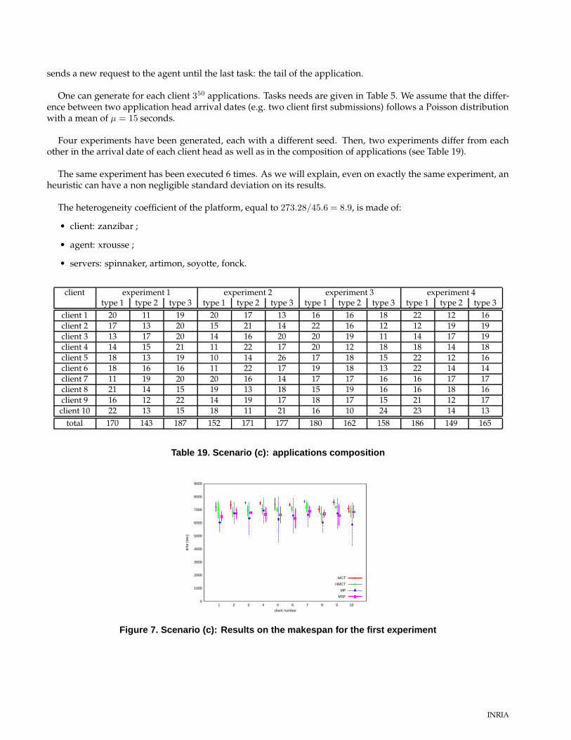
sends a new request to the agent until the last task: the tail of the application.
One can generate for each client 350 applications. Tasks needs are given in Table 5. We assume that the differ-ence between two application head arrival dates (e.g. two client first submissions) follows a Poisson distributionwith a mean of µ = 15 seconds.
Four experiments have been generated, each with a different seed. Then, two experiments differ from eachother in the arrival date of each client head as well as in the composition of applications (see Table 19).
The same experiment has been executed 6 times. As we will explain, even on exactly the same experiment, anheuristic can have a non negligible standard deviation on its results.
The heterogeneity coefficient of the platform, equal to 273.28/45.6 = 8.9, is made of:
• client: zanzibar ;
• agent: xrousse ;
• servers: spinnaker, artimon, soyotte, fonck.
client experiment 1 experiment 2 experiment 3 experiment 4type 1 type 2 type 3 type 1 type 2 type 3 type 1 type 2 type 3 type 1 type 2 type 3
client 1 20 11 19 20 17 13 16 16 18 22 12 16client 2 17 13 20 15 21 14 22 16 12 12 19 19client 3 13 17 20 14 16 20 20 19 11 14 17 19client 4 14 15 21 11 22 17 20 12 18 18 14 18client 5 18 13 19 10 14 26 17 18 15 22 12 16client 6 18 16 16 11 22 17 19 18 13 22 14 14client 7 11 19 20 20 16 14 17 17 16 16 17 17client 8 21 14 15 19 13 18 15 19 16 16 18 16client 9 16 12 22 14 19 17 18 17 15 21 12 17client 10 22 13 15 18 11 21 16 10 24 23 14 13
total 170 143 187 152 171 177 180 162 158 186 149 165
Table 19. Scenario (c): applications composition
0
1000
2000
3000
4000
5000
6000
7000
8000
9000
10987654321
time
(sec
)
client number
MCT
HMCT
MP
MSF
Figure 7. Scenario (c): Results on the makespan for the first experiment
INRIA
0
1000
2000
3000
4000
5000
6000
7000
8000
10987654321tim
e (s
ec)
client number
MCT
HMCT
MP
MSF
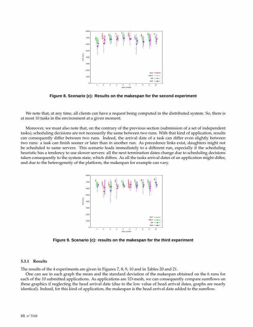
Figure 8. Scenario (c): Results on the makespan for the second experiment
We note that, at any time, all clients can have a request being computed in the distributed system. So, there isat most 10 tasks in the environment at a given moment.
Moreover, we must also note that, on the contrary of the previous section (submission of a set of independenttasks), scheduling decisions are not necessarily the same between two runs. With that kind of application, resultscan consequently differ between two runs. Indeed, the arrival date of a task can differ even slightly betweentwo runs: a task can finish sooner or later than in another run. As precedence links exist, daughters might notbe scheduled to same servers. This scenario leads immediately to a different run, especially if the schedulingheuristic has a tendency to use slower servers: all the next termination dates change due to scheduling decisionstaken consequently to the system state, which differs. As all the tasks arrival dates of an application might differ,and due to the heterogeneity of the platform, the makespan for example can vary.
0
1000
2000
3000
4000
5000
6000
7000
8000
10987654321
time
(sec
)
client number
MCT
HMCT
MP
MSF
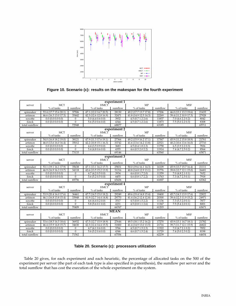
Figure 9. Scenario (c): results on the makespan for the third experiment
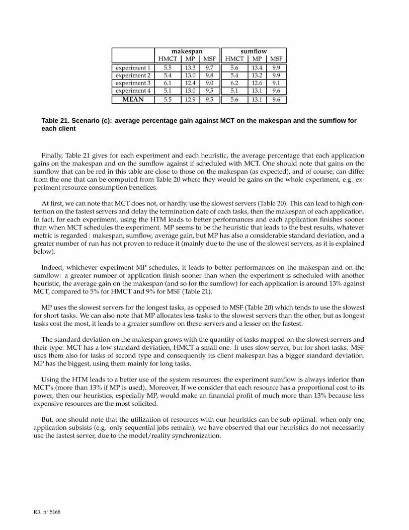
5.3.1 Results
The results of the 4 experiments are given in Figures 7, 8, 9, 10 and in Tables 20 and 21.One can see in each graph the mean and the standard deviation of the makespan obtained on the 6 runs for
each of the 10 submitted applications. As applications are 1D-mesh, we can consequently compare sumflows onthese graphics if neglecting the head arrival date (due to the low value of head arrival dates, graphs are nearlyidentical). Indeed, for this kind of application, the makespan is the head arrival date added to the sumflow.
RR n° 5168
0
1000
2000
3000
4000
5000
6000
7000
8000
10987654321tim
e (s
ec)
client number
MCT
HMCT
MP
MSF
Figure 10. Scenario (c): results on the makespan for the fourth experiment
experiment 1server MCT HMCT MP MSF
% of tasks sumflow % of tasks sumflow % of tasks sumflow % of tasks sumflowspinnaker 53.4 (17.7 15.6 20.1) 37506 47.1 (12.0 14.7 20.5) 28130 49.2 (17.7 13.7 17.8) 17206 46.0 (13.1 13.3 19.6) 21433artimon 46.6 (16.3 13.0 17.3) 35442 42.3 (12.6 12.8 16.9) 32471 41.8 (14.9 12.5 14.3) 22269 39.4 (11.2 10.9 17.3) 27928soyotte 0.0 (0.0 0.0 0.0) 0 5.0 (4.4 0.6 0.0) 3932 4.5 (0.7 1.2 2.6) 11837 7.0 (4.6 2.2 0.2) 8042fonck 0.0 (0.0 0.0 0.0) 0 5.6 (5.0 0.6 0.0) 4344 4.5 (0.7 1.2 2.6) 11873 7.5 (5.0 2.2 0.3) 8308
total sumflow 72948 68877 63185 65711experiment 2
server MCT HMCT MP MSF% of tasks sumflow % of tasks sumflow % of tasks sumflow % of tasks sumflow
spinnaker 54.0 (16.8 18.2 19.0) 38121 47.9 (11.3 17.6 19.1) 27366 49.2 (15.9 16.2 17.1) 17367 45.9 (11.2 15.8 18.9) 21761artimon 46.0 (13.6 16.0 16.4) 35012 42.2 (10.8 15.1 16.3) 33742 41.6 (13.6 14.2 13.8) 22521 40.2 (10.6 13.6 16.0) 27710soyotte 0.0 (0.0 0.0 0.0) 0 4.4 (3.5 0.9 0.0) 3683 4.5 (0.4 1.8 2.3) 11758 6.5 (3.9 2.2 0.3) 7836fonck 0.0 (0.0 0.0 0.0) 0 5.4 (4.8 0.6 0.0) 4355 4.6 (0.5 2.0 2.2) 11914 7.4 (4.7 2.5 0.2) 8564
total sumflow 73133 69146 63560 65871experiment 3
server MCT HMCT MP MSF% of tasks sumflow % of tasks sumflow % of tasks sumflow % of tasks sumflow
spinnaker 53.1 (19.1 16.1 17.9) 35638 47.1 (13.1 16.2 17.7) 25831 50.0 (19.6 16.1 14.3) 16109 45.9 (13.7 15.7 16.4) 21111artimon 46.9 (16.9 16.3 13.7) 34118 42.6 (13.5 15.2 13.9) 31216 40.8 (14.8 12.9 13.1) 21776 39.8 (12.7 12.1 15.0) 26681soyotte 0.0 (0.0 0.0 0.0) 0 4.7 (4.2 0.5 0.0) 3934 4.6 (0.8 1.7 2.0) 11359 7.0 (4.8 2.1 0.1) 7652fonck 0.0 (0.0 0.0 0.0) 0 5.6 (5.2 0.5 0.0) 4455 4.6 (0.8 1.7 2.2) 11763 7.3 (4.7 2.5 0.1) 7918
total sumflow 69756 65436 61007 63362experiment 4
server MCT HMCT MP MSF% of tasks sumflow % of tasks sumflow % of tasks sumflow % of tasks sumflow
spinnaker 53.9 (20.4 16.0 17.6) 36461 47.7 (14.5 15.0 18.2) 29249 49.6 (19.4 14.8 15.4) 18400 45.7 (14.3 13.9 17.6) 22822artimon 46.1 (16.8 13.8 15.4) 33948 41.9 (12.7 14.4 14.8) 29770 41.4 (16.2 12.4 12.8) 20300 39.4 (12.3 11.9 15.2) 24971soyotte 0.0 (0.0 0.0 0.0) 0 4.6 (4.4 0.2 0.0) 3517 4.5 (0.8 1.5 2.2) 11136 7.3 (5.3 2.0 0.1) 7877fonck 0.0 (0.0 0.0 0.0) 0 5.8 (5.6 0.1 0.0) 4231 4.5 (0.8 1.1 2.6) 11367 7.5 (5.4 2.0 0.1) 8001
total sumflow 70409 66767 61203 63671MEAN
server MCT HMCT MP MSF% of tasks sumflow % of tasks sumflow % of tasks sumflow % of tasks sumflow
spinnaker 53.6 (18.5 16.5 18.6) 36932 47.5 (12.7 15.9 18.9) 27644 49.5 (18.1 15.2 16.2) 17270 45.9 (13.1 14.7 18.1) 21782artimon 46.4 (15.9 14.8 15.7) 34630 42.3 (12.4 14.4 15.5) 31800 41.4 (14.9 13.0 13.5) 21716 39.7 (11.7 12.1 15.9) 26822soyotte 0.0 (0.0 0.0 0.0) 0 4.7 (4.1 0.6 0.0) 3766 4.5 (0.7 1.5 2.3) 11522 7.0 (4.7 2.1 0.2) 7852fonck 0.0 (0.0 0.0 0.0) 0 5.6 (5.2 0.4 0.0) 4346 4.6 (0.7 1.5 2.4) 11729 7.4 (5.0 2.3 0.2) 8198
total sumflow 71562 67556 62239 64654
Table 20. Scenario (c): processors utilization
Table 20 gives, for each experiment and each heuristic, the percentage of allocated tasks on the 500 of theexperiment per server (the part of each task type is also specified in parenthesis), the sumflow per server and thetotal sumflow that has cost the execution of the whole experiment on the system.
INRIA
makespanHMCT MP MSF
experiment 1 5.5 13.3 9.7experiment 2 5.4 13.0 9.8experiment 3 6.1 12.4 9.0experiment 4 5.1 13.0 9.5
MEAN 5.5 12.9 9.5
sumflowHMCT MP MSF
5.6 13.4 9.95.4 13.2 9.96.2 12.6 9.15.1 13.1 9.65.6 13.1 9.6
Table 21. Scenario (c): average percentage gain against MCT on the makespan and the sumflow foreach client
Finally, Table 21 gives for each experiment and each heuristic, the average percentage that each applicationgains on the makespan and on the sumflow against if scheduled with MCT. One should note that gains on thesumflow that can be red in this table are close to those on the makespan (as expected), and of course, can differfrom the one that can be computed from Table 20 where they would be gains on the whole experiment, e.g. ex-periment resource consumption benefices.
At first, we can note that MCT does not, or hardly, use the slowest servers (Table 20). This can lead to high con-tention on the fastest servers and delay the termination date of each tasks, then the makespan of each application.In fact, for each experiment, using the HTM leads to better performances and each application finishes soonerthan when MCT schedules the experiment. MP seems to be the heuristic that leads to the best results, whatevermetric is regarded : makespan, sumflow, average gain, but MP has also a considerable standard deviation, and agreater number of run has not proven to reduce it (mainly due to the use of the slowest servers, as it is explainedbelow).
Indeed, whichever experiment MP schedules, it leads to better performances on the makespan and on thesumflow: a greater number of application finish sooner than when the experiment is scheduled with anotherheuristic, the average gain on the makespan (and so for the sumflow) for each application is around 13% againstMCT, compared to 5% for HMCT and 9% for MSF (Table 21).
MP uses the slowest servers for the longest tasks, as opposed to MSF (Table 20) which tends to use the slowestfor short tasks. We can also note that MP allocates less tasks to the slowest servers than the other, but as longesttasks cost the most, it leads to a greater sumflow on these servers and a lesser on the fastest.
The standard deviation on the makespan grows with the quantity of tasks mapped on the slowest servers andtheir type: MCT has a low standard deviation, HMCT a small one. It uses slow server, but for short tasks. MSFuses them also for tasks of second type and consequently its client makespan has a bigger standard deviation.MP has the biggest, using them mainly for long tasks.
Using the HTM leads to a better use of the system resources: the experiment sumflow is always inferior thanMCT’s (more than 13% if MP is used). Moreover, If we consider that each resource has a proportional cost to itspower, then our heuristics, especially MP, would make an financial profit of much more than 13% because lessexpensive resources are the most solicited.
But, one should note that the utilization of resources with our heuristics can be sub-optimal: when only oneapplication subsists (e.g. only sequential jobs remain), we have observed that our heuristics do not necessarilyuse the fastest server, due to the model/reality synchronization.
RR n° 5168
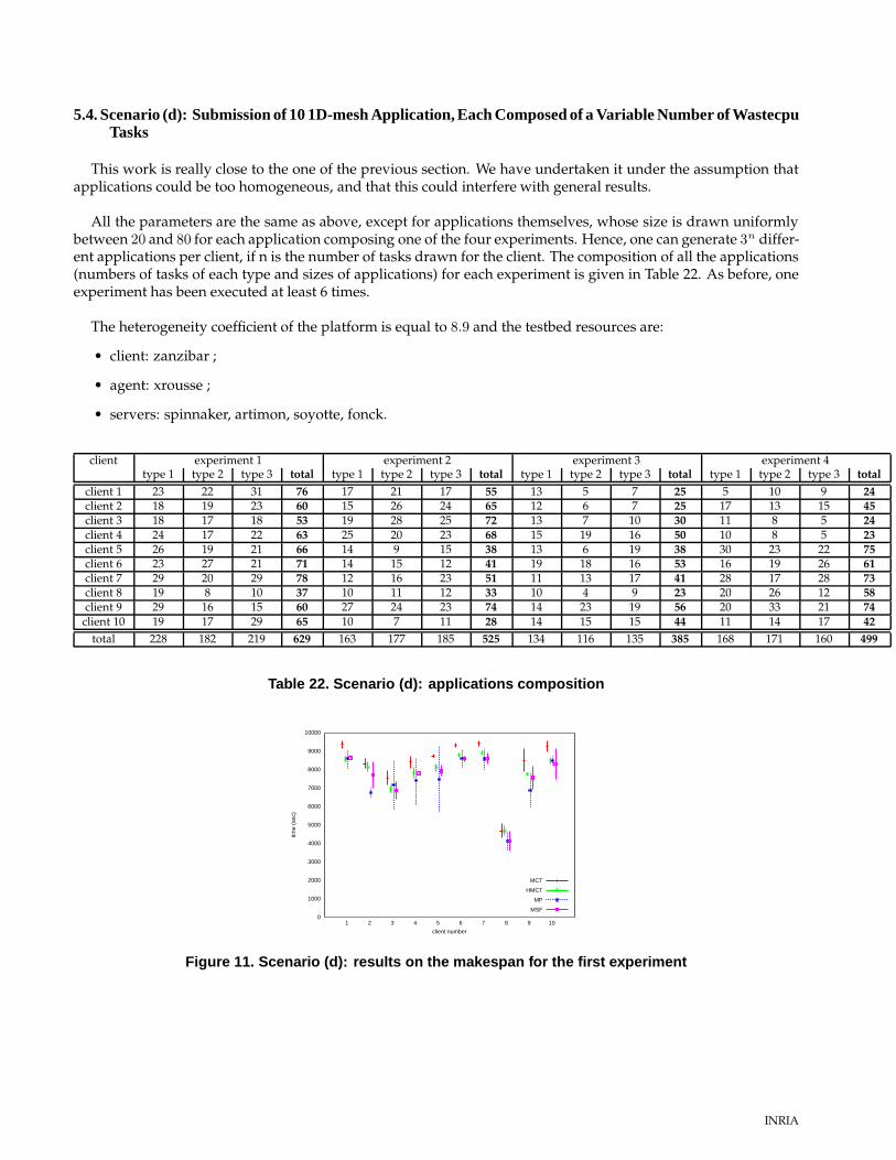
5.4. Scenario (d): Submission of 10 1D-mesh Application, Each Composed of a Variable Number of WastecpuTasks
This work is really close to the one of the previous section. We have undertaken it under the assumption thatapplications could be too homogeneous, and that this could interfere with general results.
All the parameters are the same as above, except for applications themselves, whose size is drawn uniformlybetween 20 and 80 for each application composing one of the four experiments. Hence, one can generate 3n differ-ent applications per client, if n is the number of tasks drawn for the client. The composition of all the applications(numbers of tasks of each type and sizes of applications) for each experiment is given in Table 22. As before, oneexperiment has been executed at least 6 times.
The heterogeneity coefficient of the platform is equal to 8.9 and the testbed resources are:
• client: zanzibar ;
• agent: xrousse ;
• servers: spinnaker, artimon, soyotte, fonck.
client experiment 1 experiment 2 experiment 3 experiment 4type 1 type 2 type 3 total type 1 type 2 type 3 total type 1 type 2 type 3 total type 1 type 2 type 3 total
client 1 23 22 31 76 17 21 17 55 13 5 7 25 5 10 9 24client 2 18 19 23 60 15 26 24 65 12 6 7 25 17 13 15 45client 3 18 17 18 53 19 28 25 72 13 7 10 30 11 8 5 24client 4 24 17 22 63 25 20 23 68 15 19 16 50 10 8 5 23client 5 26 19 21 66 14 9 15 38 13 6 19 38 30 23 22 75client 6 23 27 21 71 14 15 12 41 19 18 16 53 16 19 26 61client 7 29 20 29 78 12 16 23 51 11 13 17 41 28 17 28 73client 8 19 8 10 37 10 11 12 33 10 4 9 23 20 26 12 58client 9 29 16 15 60 27 24 23 74 14 23 19 56 20 33 21 74
client 10 19 17 29 65 10 7 11 28 14 15 15 44 11 14 17 42total 228 182 219 629 163 177 185 525 134 116 135 385 168 171 160 499
Table 22. Scenario (d): applications composition
0
1000
2000
3000
4000
5000
6000
7000
8000
9000
10000
10987654321
time
(sec
)
client number
MCT
HMCT
MP
MSF
Figure 11. Scenario (d): results on the makespan for the first experiment
INRIA

0
1000
2000
3000
4000
5000
6000
7000
8000
9000
10987654321tim
e (s
ec)
client number
MCT
HMCT
MP
MSF
Figure 12. Scenario (d): results on the makespan for the second experiment
0
1000
2000
3000
4000
5000
6000
7000
10987654321
time
(sec
)
client number
MCT
HMCT
MP
MSF
Figure 13. Scenario (d): results on the makespan for the third experiment
0
1000
2000
3000
4000
5000
6000
7000
8000
10987654321
time
(sec
)
client number
MCT
HMCT
MP
MSF
Figure 14. Scenario (d): results on the makespan for the fourth experiment
5.4.1 Results
Results of the 4 experiments are given in Figures 11, 12, 13, 14 and in Tables 23 and 24.One can see in each graph the mean and the standard deviation of the makespan obtained on the 6 runs of each
of the 10 submitted applications. Like explained in the previous section, since applications are 1D-mesh, graphs
RR n° 5168

of application sumflows are nearly identical to those for the makespan. Then, commentaries on applicationsmakespans are valid for applications sumflows.
Table 23 gives, for each experiment and each heuristic: the percentage per server of allocated tasks (the per-centage per type is also specified in parenthesis) on the number of tasks of the given experiment (which is givenin Table 22) ; the sumflow per server and the total sumflow that has cost the whole experiment on the system.
At last, Table 24 gives the average percentage gain that each application gains on the makespan and on thesumflow if scheduled with our heuristics against MCT.
experiment 1server MCT HMCT MP MSF
% of tasks sumflow % of tasks sumflow % of tasks sumflow % of tasks sumflowspinnaker 53.6 (18.8 15.7 19.1) 43246 47.8 (13.9 14.0 19.9) 31757 50.2 (18.7 15.1 16.5) 20456 44.7 (13.0 13.5 18.2) 24223artimon 46.4 (17.4 13.3 15.7) 38815 40.5 (12.0 13.9 14.6) 34357 40.5 (15.3 11.6 13.7) 24129 40.9 (14.5 10.9 15.5) 28759soyotte 0.0 (0.0 0.0 0.0) 0 5.3 (4.5 0.6 0.2) 5374 4.6 (1.2 0.9 2.5) 14770 7.1 (4.6 2.0 0.5) 10544fonck 0.0 (0.0 0.0 0.0) 0 6.4 (5.9 0.4 0.1) 6103 4.6 (1.1 1.4 2.1) 14001 7.4 (4.2 2.5 0.6) 11477
total sumflow 82061 77591 73356 75003experiment 2
server MCT HMCT MP MSF% of tasks sumflow % of tasks sumflow % of tasks sumflow % of tasks sumflow
spinnaker 54.5 (17.0 18.4 19.0) 35248 49.1 (13.1 16.7 19.3) 28022 50.5 (16.4 17.5 16.6) 17733 46.3 (10.8 16.9 18.7) 22008artimon 45.5 (14.0 15.3 16.2) 31211 42.4 (9.8 16.7 15.9) 29492 41.6 (14.0 13.6 14.0) 20934 39.5 (10.6 12.7 16.3) 23671soyotte 0.0 (0.0 0.0 0.0) 0 3.5 (3.5 0.0 0.0) 2474 3.4 (0.0 1.0 2.5) 9557 7.0 (4.7 2.2 0.1) 7420fonck 0.0 (0.0 0.0 0.0) 0 5.0 (4.6 0.4 0.0) 3665 4.5 (0.7 1.6 2.2) 11375 7.2 (5.0 2.0 0.2) 7486
total sumflow 66459 63653 59599 60585experiment 3
server MCT HMCT MP MSF% of tasks sumflow % of tasks sumflow % of tasks sumflow % of tasks sumflow
spinnaker 54.4 (19.7 16.2 18.4) 24492 51.2 (16.2 16.1 18.8) 20973 49.7 (18.1 14.9 16.8) 13027 46.5 (13.8 13.8 19.0) 15796artimon 45.6 (15.1 13.9 16.6) 22175 44.3 (14.0 14.0 16.2) 21776 41.3 (15.6 12.1 13.6) 13389 38.4 (9.0 13.4 16.1) 16904soyotte 0.0 (0.0 0.0 0.0) 0 1.4 (1.4 0.0 0.0) 708 4.5 (0.6 1.8 2.1) 7631 7.3 (5.8 1.4 0.0) 4648fonck 0.0 (0.0 0.0 0.0) 0 3.1 (3.1 0.0 0.0) 1537 4.4 (0.5 1.3 2.6) 7566 7.8 (6.2 1.6 0.0) 5026
total sumflow 46667 44994 41613 42374
experiment 4server MCT HMCT MP MSF
% of tasks sumflow % of tasks sumflow % of tasks sumflow % of tasks sumflowspinnaker 54.7 (19.0 19.0 16.6) 30543 48.9 (13.5 17.5 17.8) 24356 49.2 (17.8 16.2 15.1) 15402 46.3 (12.6 15.9 17.7) 18488artimon 45.3 (14.6 15.2 15.4) 25555 43.8 (12.8 16.7 14.2) 25334 41.7 (14.8 14.0 12.8) 16013 40.6 (11.8 14.5 14.2) 19653soyotte 0.0 (0.0 0.0 0.0) 0 2.7 (2.7 0.0 0.0) 1750 4.5 (0.5 1.9 2.1) 9848 6.0 (4.0 1.9 0.1) 5725fonck 0.0 (0.0 0.0 0.0) 0 4.6 (4.6 0.0 0.0) 2978 4.6 (0.5 2.1 2.0) 10226 7.1 (5.2 1.9 0.0) 6462
total sumflow 56098 54418 51489 50328MEAN
server MCT HMCT MP MSF% of tasks sumflow % of tasks sumflow % of tasks sumflow % of tasks sumflow
spinnaker 54.3 (18.7 17.3 18.3) 33382 49.2 (14.2 16.1 19.0) 26277 49.9 (17.7 15.9 16.2) 16654 45.9 (12.5 15.0 18.4) 20129artimon 45.7 (15.3 14.4 16.0) 29439 42.7 (12.2 15.3 15.2) 27740 41.3 (14.9 12.8 13.5) 18616 39.9 (11.5 12.9 15.5) 22247soyotte 0.0 (0.0 0.0 0.0) 0 3.2 (3.0 0.2 0.1) 2576 4.3 (0.6 1.4 2.3) 10452 6.8 (4.8 1.9 0.2) 7084fonck 0.0 (0.0 0.0 0.0) 0 4.8 (4.5 0.2 0.0) 3571 4.5 (0.7 1.6 2.2) 10792 7.4 (5.2 2.0 0.2) 7613
total sumflow 62821 60164 56514 57072
Table 23. Scenario (d): processors utilization
Same conclusions than in the previous section can be made here, even if sizes of applications are different fromeach other. MCT does not use any of the SUN servers because of their slow computation power, and gives theworst results whatever the considered metric is. This was expectable: because applications costs are more hetero-geneous that before, the throughput is not constantly high. MCT has even less the need of slower servers.
Using MP is not as good as before, but is still the best on average regardless the metric (even slightly againstMSF). One can also note that the standard deviation is smaller for all heuristics and especially for MP, althoughservers utilization is quiet identical: the lower throughput hence the lower contention on servers is the reasonthat explains these two facts.
Indeed, we can observe in Table 23 the same behaviour of the heuristics than in the previous section. MPmappes longer tasks to slower servers, HMCT uses them only to compute short tasks, and MSF avoids to allocate
INRIA
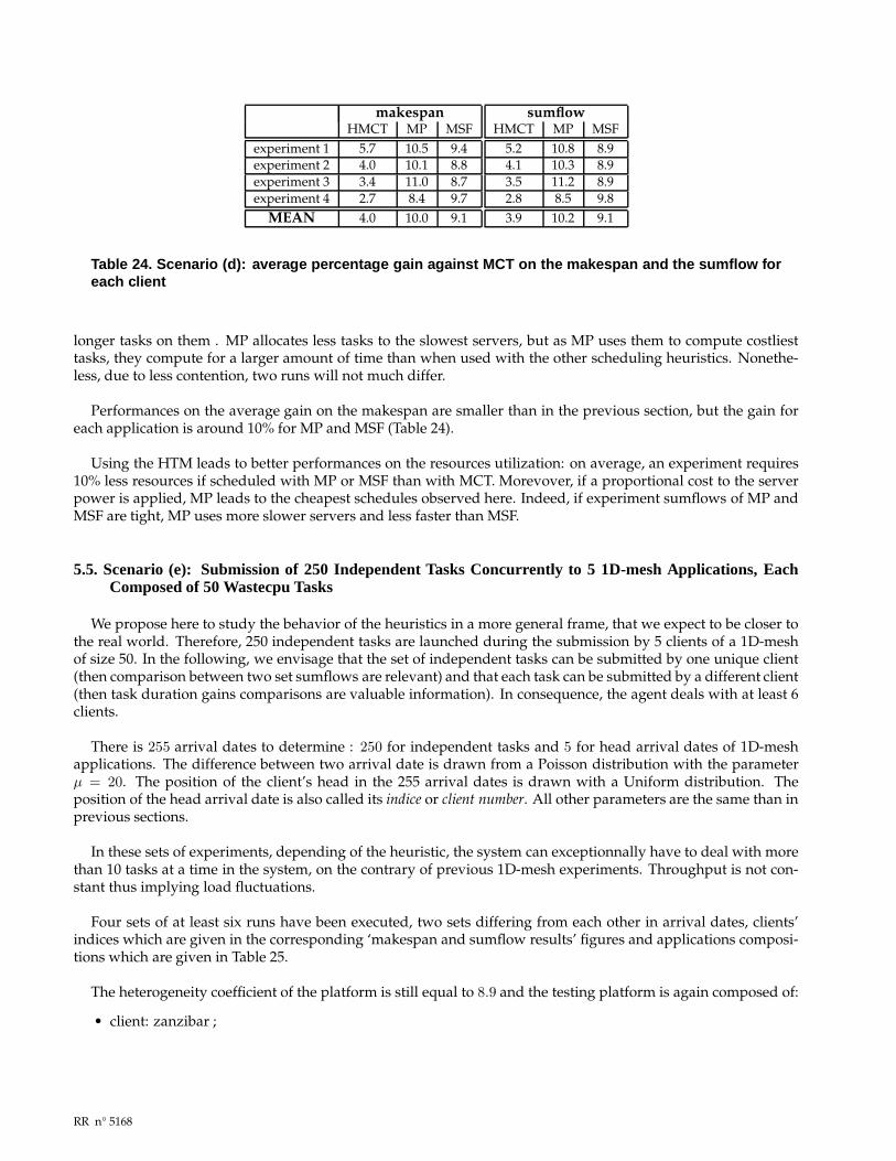
makespanHMCT MP MSF
experiment 1 5.7 10.5 9.4experiment 2 4.0 10.1 8.8experiment 3 3.4 11.0 8.7experiment 4 2.7 8.4 9.7
MEAN 4.0 10.0 9.1
sumflowHMCT MP MSF
5.2 10.8 8.94.1 10.3 8.93.5 11.2 8.92.8 8.5 9.83.9 10.2 9.1
Table 24. Scenario (d): average percentage gain against MCT on the makespan and the sumflow foreach client
longer tasks on them . MP allocates less tasks to the slowest servers, but as MP uses them to compute costliesttasks, they compute for a larger amount of time than when used with the other scheduling heuristics. Nonethe-less, due to less contention, two runs will not much differ.
Performances on the average gain on the makespan are smaller than in the previous section, but the gain foreach application is around 10% for MP and MSF (Table 24).
Using the HTM leads to better performances on the resources utilization: on average, an experiment requires10% less resources if scheduled with MP or MSF than with MCT. Morevover, if a proportional cost to the serverpower is applied, MP leads to the cheapest schedules observed here. Indeed, if experiment sumflows of MP andMSF are tight, MP uses more slower servers and less faster than MSF.
5.5. Scenario (e): Submission of 250 Independent Tasks Concurrently to 5 1D-mesh Applications, EachComposed of 50 Wastecpu Tasks
We propose here to study the behavior of the heuristics in a more general frame, that we expect to be closer tothe real world. Therefore, 250 independent tasks are launched during the submission by 5 clients of a 1D-meshof size 50. In the following, we envisage that the set of independent tasks can be submitted by one unique client(then comparison between two set sumflows are relevant) and that each task can be submitted by a different client(then task duration gains comparisons are valuable information). In consequence, the agent deals with at least 6clients.
There is 255 arrival dates to determine : 250 for independent tasks and 5 for head arrival dates of 1D-meshapplications. The difference between two arrival date is drawn from a Poisson distribution with the parameterµ = 20. The position of the client’s head in the 255 arrival dates is drawn with a Uniform distribution. Theposition of the head arrival date is also called its indice or client number. All other parameters are the same than inprevious sections.
In these sets of experiments, depending of the heuristic, the system can exceptionnally have to deal with morethan 10 tasks at a time in the system, on the contrary of previous 1D-mesh experiments. Throughput is not con-stant thus implying load fluctuations.
Four sets of at least six runs have been executed, two sets differing from each other in arrival dates, clients’indices which are given in the corresponding ‘makespan and sumflow results’ figures and applications composi-tions which are given in Table 25.
The heterogeneity coefficient of the platform is still equal to 8.9 and the testing platform is again composed of:
• client: zanzibar ;
RR n° 5168
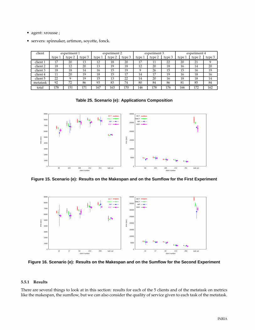
• agent: xrousse ;
• servers: spinnaker, artimon, soyotte, fonck.
client experiment 1 experiment 2 experiment 3 experiment 4type 1 type 2 type 3 type 1 type 2 type 3 type 1 type 2 type 3 type 1 type 2 type 3
client 1 17 20 13 12 18 20 17 11 22 20 21 9client 2 18 12 20 13 19 18 12 20 18 16 14 20client 3 18 18 14 16 15 19 9 26 15 15 16 19client 4 11 20 19 18 15 17 14 17 19 16 18 16client 5 22 9 19 15 13 22 14 20 16 18 18 14
metatask 92 72 86 93 83 74 80 84 86 81 85 84total 178 151 171 167 163 170 146 178 176 166 172 162
Table 25. Scenario (e): Applications Composition
0
1000
2000
3000
4000
5000
6000
7000
8000
9000
90 103 186 212 251 task set
time
(sec
)
client number
MCT
HMCT
MP
MSF
0
5000
10000
15000
20000
25000
30000
task set25121218610390
time
(sec
)
client number
MCT
HMCT
MP
MSF
Figure 15. Scenario (e): Results on the Makespan and on the Sumflow for the First Experiment
0
1000
2000
3000
4000
5000
6000
7000
8000
9000
14 17 64 213 250 task set
time
(sec
)
client number
MCT
HMCT
MP
MSF
0
5000
10000
15000
20000
25000
30000
35000
40000
task set250213641714
time
(sec
)
client number
MCT
HMCT
MP
MSF
Figure 16. Scenario (e): Results on the Makespan and on the Sumflow for the Second Experiment
5.5.1 Results
There are several things to look at in this section: results for each of the 5 clients and of the metatask on metricslike the makespan, the sumflow, but we can also consider the quality of service given to each task of the metatask.
INRIA
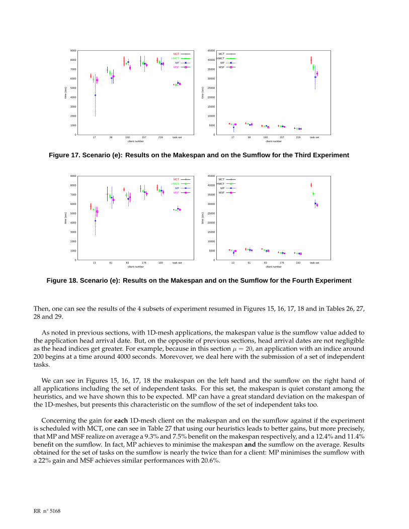
0
1000
2000
3000
4000
5000
6000
7000
8000
9000
17 38 150 157 219 task set
time
(sec
)
client number
MCT
HMCT
MP
MSF
0
5000
10000
15000
20000
25000
30000
35000
40000
45000
task set2191571503817
time
(sec
)
client number
MCT
HMCT
MP
MSF
Figure 17. Scenario (e): Results on the Makespan and on the Sumflow for the Third Experiment
0
1000
2000
3000
4000
5000
6000
7000
8000
9000
13 61 83 176 193 task set
time
(sec
)
client number
MCT
HMCT
MP
MSF
0
5000
10000
15000
20000
25000
30000
35000
40000
45000
task set193176836113
time
(sec
)
client number
MCT
HMCT
MP
MSF
Figure 18. Scenario (e): Results on the Makespan and on the Sumflow for the Fourth Experiment
Then, one can see the results of the 4 subsets of experiment resumed in Figures 15, 16, 17, 18 and in Tables 26, 27,28 and 29.
As noted in previous sections, with 1D-mesh applications, the makespan value is the sumflow value added tothe application head arrival date. But, on the opposite of previous sections, head arrival dates are not negligibleas the head indices get greater. For example, because in this section µ = 20, an application with an indice around200 begins at a time around 4000 seconds. Morevover, we deal here with the submission of a set of independenttasks.
We can see in Figures 15, 16, 17, 18 the makespan on the left hand and the sumflow on the right hand ofall applications including the set of independent tasks. For this set, the makespan is quiet constant among theheuristics, and we have shown this to be expected. MP can have a great standard deviation on the makespan ofthe 1D-meshes, but presents this characteristic on the sumflow of the set of independent taks too.
Concerning the gain for each 1D-mesh client on the makespan and on the sumflow against if the experimentis scheduled with MCT, one can see in Table 27 that using our heuristics leads to better gains, but more precisely,that MP and MSF realize on average a 9.3% and 7.5% benefit on the makespan respectively, and a 12.4% and 11.4%benefit on the sumflow. In fact, MP achieves to minimise the makespan and the sumflow on the average. Resultsobtained for the set of tasks on the sumflow is nearly the twice than for a client: MP minimises the sumflow witha 22% gain and MSF achieves similar performances with 20.6%.
RR n° 5168
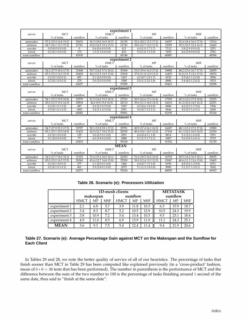
experiment 1server MCT HMCT MP MSF
% of tasks sumflow % of tasks sumflow % of tasks sumflow % of tasks sumflowspinnaker 55.2 (19.4 16.8 19.0) 25676 54.3 (18.8 16.8 18.7) 22159 52.6 (20.2 15.2 17.2) 14057 52.4 (18.4 16.0 17.9) 17014artimon 44.7 (16.1 13.3 15.2) 21781 43.8 (14.9 13.4 15.5) 21743 38.0 (12.7 12.0 13.3) 12059 39.2 (10.5 12.4 16.3) 16460soyotte 0.0 (0.0 0.0 0.0) 0 0.6 (0.6 0.0 0.0) 413 4.4 (1.0 1.7 1.7) 7112 3.8 (2.9 0.9 0.0) 3251fonck 0.2 (0.1 0.0 0.0) 173 1.3 (1.3 0.0 0.0) 833 5.0 (1.8 1.3 2.0) 7659 4.6 (3.8 0.8 0.0) 3781
total sumflow 47630 45148 40887 40506experiment 2
server MCT HMCT MP MSF% of tasks sumflow % of tasks sumflow % of tasks sumflow % of tasks sumflow
spinnaker 54.2 (17.9 18.4 17.9) 31848 50.7 (14.8 17.6 18.2) 30368 53.0 (19.6 16.0 17.4) 18888 48.2 (13.6 16.7 17.9) 24095artimon 45.3 (15.2 14.2 15.9) 30428 44.2 (13.5 14.9 15.8) 23818 37.8 (11.8 12.8 13.2) 14495 41.0 (11.5 13.6 15.9) 18074soyotte 0.2 (0.1 0.0 0.1) 491 2.1 (2.0 0.0 0.0) 1415 4.2 (0.7 1.8 1.7) 8152 5.5 (4.3 1.2 0.0) 5096fonck 0.2 (0.1 0.0 0.1) 270 3.0 (3.0 0.0 0.0) 1988 5.0 (1.3 2.0 1.8) 8886 5.4 (4.0 1.2 0.2) 5033
total sumflow 63037 57589 50421 52298experiment 3
server MCT HMCT MP MSF% of tasks sumflow % of tasks sumflow % of tasks sumflow % of tasks sumflow
spinnaker 54.1 (15.5 19.8 18.8) 33579 51.5 (14.0 19.2 18.3) 27253 50.9 (16.6 17.6 16.8) 17259 49.2 (12.6 17.8 18.8) 21923artimon 45.0 (13.5 15.6 16.0) 29834 42.6 (9.8 15.8 16.9) 28110 39.6 (11.3 14.0 14.3) 16610 41.2 (10.4 14.5 16.3) 22291soyotte 0.4 (0.1 0.1 0.2) 487 2.6 (2.3 0.3 0.0) 1947 4.5 (0.6 1.8 2.0) 8680 4.6 (2.9 1.7 0.0) 5306fonck 0.5 (0.1 0.1 0.3) 1083 3.4 (3.1 0.3 0.0) 2591 5.0 (0.7 2.2 2.1) 9646 5.0 (3.3 1.6 0.1) 5640
total sumflow 64983 59901 52195 55160experiment 4
server MCT HMCT MP MSF% of tasks sumflow % of tasks sumflow % of tasks sumflow % of tasks sumflow
spinnaker 54.7 (17.9 19.3 17.5) 33797 50.1 (13.8 19.1 17.2) 25791 49.9 (17.4 16.1 16.5) 16607 48.1 (13.2 17.2 17.8) 19589artimon 45.1 (15.1 15.0 14.9) 31432 42.9 (12.7 15.0 15.2) 28330 40.6 (14.1 14.5 12.0) 17104 41.1 (12.6 14.0 14.5) 21034soyotte 0.2 (0.1 0.0 0.0) 129 3.0 (2.9 0.1 0.0) 2091 4.4 (0.4 2.1 1.8) 8814 5.2 (3.6 1.6 0.0) 5391fonck 0.1 (0.0 0.0 0.0) 77 4.0 (3.8 0.2 0.0) 2888 5.1 (1.3 1.7 2.1) 9407 5.6 (3.8 1.6 0.1) 5715
total sumflow 65435 59100 51932 51729MEAN
server MCT HMCT MP MSF% of tasks sumflow % of tasks sumflow % of tasks sumflow % of tasks sumflow
spinnaker 54.5 (17.7 18.6 18.3) 31225 51.6 (15.4 18.2 18.1) 26393 51.6 (18.5 16.2 16.9) 16703 49.5 (14.4 16.9 18.1) 20655artimon 45.0 (15.0 14.5 15.5) 28369 43.4 (12.7 14.8 15.8) 25500 39.0 (12.4 13.3 13.2) 15067 40.6 (11.2 13.6 15.8) 19465soyotte 0.2 (0.1 0.0 0.1) 277 2.1 (2.0 0.1 0.0) 1466 4.4 (0.7 1.9 1.8) 8190 4.8 (3.4 1.3 0.0) 4761fonck 0.2 (0.1 0.1 0.1) 401 2.9 (2.8 0.1 0.0) 2075 5.1 (1.3 1.8 2.0) 8900 5.1 (3.7 1.3 0.1) 5042
total sumflow 60271 55434 48859 49923
Table 26. Scenario (e): Processors Utilization
1D-mesh clientsmakespan sumflow
HMCT MP MSF HMCT MP MSFexperiment 1 2.1 6.8 5.7 3.9 11.8 10.3experiment 2 3.4 8.3 8.7 5.2 10.5 12.9experiment 3 3.8 10.9 7.2 5.4 13.4 10.5experiment 4 4.9 11.0 8.5 6.9 13.9 11.9
MEAN 3.6 9.3 7.5 5.4 12.4 11.4
METATASKsumflow
HMCT MP MSF6.3 15.9 18.7
10.5 24.3 19.99.5 23.1 18.4
11.1 24.3 25.19.4 21.9 20.6
Table 27. Scenario (e): Average Percentage Gain against MCT on the Makespan and the Sumflow forEach Client
In Tables 29 and 28, we note the better quality of service of all of our heuristics. The percentage of tasks thatfinish sooner than MCT in Table 29 has been computed like explained previously (in a ‘cross-product’ fashion,mean of 6 ∗ 6 = 36 tests that has been performed). The number in parenthesis is the performance of MCT and thedifference between the sum of the two number to 100 is the percentage of tasks finishing around 1 second of thesame date, thus said to “finish at the same date”.
INRIA

mean flow gain in percentageMCT (sec) HMCT MP MSF
type 1 53.4 1.0 21.7 0.6experiment 1 type 2 104.0 10.9 17.7 19.0
type 3 164.6 5.7 13.0 24.8type 1 77.9 -0.6 29.5 -6.0
experiment 2 type 2 160.9 12.1 17.2 20.2type 3 241.3 15.0 30.0 30.6type 1 76.7 -2.9 32.5 -7.4
experiment 3 type 2 151.4 11.9 14.7 12.7type 3 244.2 11.3 25.0 28.8type 1 80.0 -1.9 31.9 4.5
experiment 4 type 2 170.1 15.6 20.2 27.4type 3 228.5 12.8 25.3 33.6
MEAN - 146.1 7.6 23.2 15.7
Table 28. Scenario (e): Average Percentage Gain for µ = 20 sec on Each Task Given by Type
We can see that our heuristics lead always to more tasks that finish soonner, and bests results are obtained forMP which achieves to place 80% of tasks that finish sooner than if scheduled with MCT. Still on the average, 5%of tasks finish ‘at the same date’. Nonetheless, neither MP nor MSF beat MCT on the maxtretch, e.g. the worstcase delay proportionnally to the time a task requires on the same server. Still, MCT beats MP on the maxflow,but MSF performs better (and HMCT even better).
To confirm the quality of the previous results, one can see in Table 28, for each type of task and each experiment,the mean flow obtained when the task has been scheduled with MCT. On the same line is given the percentage ofgain on the duration of the task when the experiment is scheduled with the given heuristic.
Each independent task is 23% or 15.7% shorter if using MP or MSF. One can also note that using the HTM withHMCT lead to improve the scheduling: better quality of service and better makespan and sumflow regardless theclient.
At last, one can see the experiments cost with the detailed sumflow values in Table 26. Our heuristics givebetter results, and MP beats the other on the average. We can observe that MP uses slower servers to preferablyscheduled average and long duration tasks (type 2 and 3). This leads to higher sumflows on slowest servers evenif less tasks than with MSF are mapped on them. On the opposite, HMCT and MSF compute a larger part of type1 tasks on them than other type. The heuristic behavior is identical to the one that has been observed in previousscenarios.
Finally, on a financial point of vue, as faster servers usage costs normally more than slower ones, MP minimisesthe cost of the experiment. Because tasks that are mapped to slower servers are at least of average duration, thetime required on these servers can be considered as huge against MCT’s (8900 seconds on fonck for MP against401 seconds for MCT in average), but also cheaper than the cost of the difference between the sumflow utilizedon faster servers (16703 seconds on spinnaker for MP against 31225 seconds for MCT, hence half the cost).
RR n° 5168

NetSolve’s MCT HMCT MP MSFseed1 seed2 seed3 seed4 Avg seed1 seed2 seed3 seed4 Avg seed1 seed2 seed3 seed4 Avg seed1 seed2 seed3 seed4 Avg
makespan 5377 5302 5350 5383 5353 5315 5148 5337 5340 5285 5448 5393 5544 5505 5472 5393 5254 5429 5399 5369
sumflow 26559 38461 39850 40133 36251 24888 34204 36138 35534 32691 22333 28669 30732 30294 28007 21594 30739 32649 29435 28604
maxflow 363.2 464.9 561.0 397.4 446.6 312.8 303.3 381.9 331.0 332.2 549.2 658.5 656.5 651.3 628.9 318.4 409.3 454.0 395.1 394.2
maxstretch 11.0 11.7 13.8 10.0 11.6 9.1 11.2 13.3 11.7 11.4 14.7 17.1 17.8 18.3 17.0 13.5 16.2 18.3 17.2 16.3
percentageof tasks - - - - − 53 (34) 61 (36) 62 (34) 64 (32) 60(34) 72 (16) 85 (14) 82 (15) 83 (14) 80(15) 65 (22) 71 (26) 72 (25) 76 (21) 71(24)
that finishsooner thanwith MCT
Table 29. Scenario (e) :Results in Seconds for µ = 20 sec on Wastecpu Tasks
INR
IA

5.6. Scenarios (f,g,h,i,j): Submissions Containing a Stencil Application
The kernel of a stencil application is given in Figure 6. Each of its tasks have same needs, and so require thesame amount of time. We present in this section different scenarios: submissions of a stencil application composedof tasks of type 1 then of type 3 ; submissions of a stencil application in parallel of a independent tasks submittedat two different rates and finally the submission of a smaller stencil graph concurrently to independent tasks.
Firstly, we point on some remarks on the common experiments background.
5.6.1 Notes
Relying on [BBR01], a stencil application in this work is composed of one type of task. It is composed of 10 or 5tasks width and the depth of the graph is also given in the corresponding subsection (50 for the first, 25 for theother).
When a client begins to request the agent for its stencil, width tasks are submitted. If no independent task issubmitted in parallel, a maximum of width tasks can be present in the system at a time. In the following, and aswritten in Figure 6, we refer by the task (i,j) to the task which is on the ith line and jth column.
"synchronization barrier"
task scheduled on a slowserver
task scheduled on a fastserver
Figure 19. Example of a 10x8 stencil application execution
The agent can have to theorically face a set of requests (10 at the beginning of the submission for example). Butin reality, the agent receives them in a given order. There are two remarks to do on that point: firstly, the submis-sion is implementation dependant. That means that the client can try to force tasks that are higher in the graph tobe submitted first in the pool of the ready tasks (tasks are submitted in a “lexical order” with the (i,j) information)but other submission orders can be made. We have chosen the first implementation. Second, because of the clientsystem (scheduling of threads and fork processes) or network problems (congestion), requests can be validatedby the agent in a different order than the one wanted by the client. Due to the experimental platform, we do nothave this problem in this work.
One should be cautious considering the results: we recall that the agent has no information on the applicationsit has to schedule. Furthermore, as one can see, this kind of graph is a priori a good counter-example for themakespan of the good behavior of MP in general and is done on purpose. Indeed, Figure 19 shows a MP scheduleof a 10*8 stencil application on a hypothetical testbed composed of 2 same fast servers and 2 same slow servers,
RR n° 5168

with the hypothesis that the heterogeneity coefficient is at least 13 (e.g. that task duration on a slow server is atleast 13 times superior to its duration on a fast one). Tasks that are assigned to slow servers are marked with adot in their center.
This example shows the main drawback of MP, that we have already explained in [CJ02]: if there are idleservers left in the system, MP chooses them to place the task. It can also use them if the perturbation is too highon the fastest servers, even if it is due to tasks that will finish in a few seconds and let the fast server idle. We willsee the effect of this scheduling strategy.
Indeed, one can easily see boundaries where faster servers are idle and wait for the ending of tasks mapped toslower ones. These boudaries give a synchronization barrier effect, and in our case, it is easy to show that they areof the same number than the depth of the graph. So MP is particularly targeted with that kind of kernel.
In the following sections, we have an heterogeneity of 8.9, and the testing environment is made with thefollowing servers:
• client: zanzibar ;
• agent: xrousse ;
• servers: spinnaker, artimon, soyotte, fonck.
5.6.2 Scenarios (f) and (g): Submission a Stencil Applications, Consequences of the Task Type
We consider in this section 2 submissions of a 10*50 stencil application: the first one composed of tasks of type 1and the second of tasks of type 3.
Scenario (f): 10*50 Stencil Composed of Tasks of Type 1The type of task involved in this scenario is the first one: the stencil is only made of the shortest duration tasktype (tasks durations are given in Table 5).
Makespan and sumflow graphs are given in Figure 20 and the detailed sumflow per server can be found inTable 30.
One can see that MP gives a higher makespan than MCT but minimises the sumflow: this is explained later.MSF minimises the makespan and behaves the same along the runs: the standard deviation for the makespan isvery low. It outperforms MCT with nearly half the sumflow.
We can also see the different behavior of MCT which uses more artimon than spinnaker (see Table 30. Thisis mainly because of the lack of precision of task durations which are computed with the load average sent bythe servers and corrected by the load correction mechanisms. On the opposite, HMCT which uses slower serversbehaves like usual when there is perturbation.
0
1000
2000
3000
4000
5000
6000
7000
1
time
(sec
)
client number
MCT
HMCT
MP
MSF
0
5000
10000
15000
20000
25000
30000
35000
40000
45000
1
time
(sec
)
client number
MCT
HMCT
MP
MSF
Figure 20. Scenario (f): makespan and sumflow results
INRIA

server MCT HMCT MP MSF% of tasks sumflow % of tasks sumflow % of tasks sumflow % of tasks sumflow
spinnaker 43.3 (43.3 0.0 0.0) 12383 53.3 (53.3 0.0 0.0) 18183 66.6 (66.6 0.0 0.0) 5720 50.6 (50.6 0.0 0.0) 10160artimon 56.7 (56.7 0.0 0.0) 27094 46.0 (46.0 0.0 0.0) 16065 22.2 (22.2 0.0 0.0) 2533 43.9 (43.9 0.0 0.0) 9375soyotte 0.0 (0.0 0.0 0.0) 0 0.2 (0.2 0.0 0.0) 150 2.3 (2.3 0.0 0.0) 1507 1.7 (1.7 0.0 0.0) 1115fonck 0.0 (0.0 0.0 0.0) 0 0.4 (0.4 0.0 0.0) 278 9.0 (9.0 0.0 0.0) 5805 3.7 (3.7 0.0 0.0) 2391
sumflow 39477 34676 15565 23041
Table 30. Scenario (f): servers utilization
The remark done in section 5.6.1 about the execution of the stencil application if scheduled with MP is notexactly valid here, because of the heterogeneity coefficient of 8.9. But the same kind of thing happens here (seeFigure 21):Tasks (0,2) and (0,3) are allocated to fonck and soyotte, and artimon and spinnaker receive and execute all thetasks available until tasks (2,8) and (2,9). It is interesting to see that tasks (2,8) and (2,9) are allocated to fonck andsoyotte, at time 119. It is surprising because these tasks have not yet finished, but the perturbation is minimumon these servers, and so tasks (0,2) and (0,3) are delayed in time. That’s why the scheduled plan explained insection 5.6.1 is only valid on a system with a higher heterogeneity coefficient. When tasks (2,8) and (2,9) areassigned, there is no task left to submit to the agent until tasks (0,2) and (0,3) finish at time 141. Spinnaker andartimon finish their last tasks at time 134 and 136 respectively, then they are idle at least 5 seconds. Fonck andsoyotte are chosen next to schedule tasks (3,2) and (3,3). All tasks until then are realized by the two fast servers.As before, tasks (2,8) and (2,9) were not finished, so they are delayed in time and finish finally at time 290. But,when task (4,5) finish at time 279, there is no work to do and all tasks previously assigned on the fast servers aredone. Fast servers are idle 12 seconds. This confirms the remark about MP and its possible results on this typeof kernel. But further works have to be done to conclude, because MP can still achieve an a priori good work in amulti-client system (see section 5.6.3).
This explains why MP achieves the worst makespan, but minimises the sumflow: there is less contention onfast servers thus the lower cost.
"synchronization barrier"
task scheduled on a slowserver
task scheduled on a fastserver
141
119
290
279
Figure 21. Scenario (f): schedule of MP
RR n° 5168

Scenario (g): 10*50 Stencil Composed of Tasks of Type 3Because of the duration of a run, this subset is only composed of one run. The main objective was to confirm, andit does, expected behaviours of heuristics in their tendancies regarding each metric.
The graph of the application is still composed of 10 tasks width and 50 depth, but the task type is the longestone, e.g. tasks are of type 3 (see Table 5 for more details).
Makespan and sumflow graphs are given in Figure 22 and the server utilization where information like thesumflow and the percentage of tasks scheduled per server can be found is given in Table 31.
0
2000
4000
6000
8000
10000
12000
14000
16000
18000
1
time
(sec
)
client number
MCT
HMCT
MP
MSF
0
20000
40000
60000
80000
100000
120000
1
time
(sec
)
client number
MCT
HMCT
MP
MSF
Figure 22. Scenario (g): makespan and sumflow results
server MCT HMCT MP MSF% of tasks sumflow % of tasks sumflow % of tasks sumflow % of tasks sumflow
spinnaker 46.4 (0.0 0.0 46.4) 38633 53.4 (0.0 0.0 53.4) 53743 47.8 (0.0 0.0 47.8) 13481 51.6 (0.0 0.0 51.6) 35985artimon 53.6 (0.0 0.0 53.6) 72776 46.6 (0.0 0.0 46.6) 51461 34.2 (0.0 0.0 34.2) 10498 45.0 (0.0 0.0 45.0) 34693soyotte 0.0 (0.0 0.0 0.0) 0 0.0 (0.0 0.0 0.0) 0 9.0 (0.0 0.0 9.0) 17204 0.6 (0.0 0.0 0.6) 1150fonck 0.0 (0.0 0.0 0.0) 0 0.0 (0.0 0.0 0.0) 0 9.0 (0.0 0.0 9.0) 17388 2.8 (0.0 0.0 2.8) 5343
sumflow 111409 105204 58571 77171
Table 31. Scenario (g): servers utilization
The results, if confirming the bad tendancies of MP on the makespan, are interesting for they show, on theopposite of the type 1 stencil where 66% of the tasks were assigned on spinnaker, that the slower servers are used.That means that, in this case, the “synchronization barrier effect” is radically minimized due to the duration oftasks. Indeed, the reason is the heterogeneity coefficient: 1 second of perturbation on slow servers can be seen asat least 8.9 seconds of perturbation on spinnaker.
ResultsOne can find a recapitulation of the gain realized by our heuristics against MCT on the makespan and the sum-flow in Table 5.6.2. Results show that the utilization of the HTM brings a lot in the decision making, even if onlyone application is involved: the schedule is built on top of a higher knowledge of what is done on each server.
First, one should note the same aspect of graphs for these two scenarios: we find the same behavior on themakespan and on the sumflow for both scenarios.
INRIA
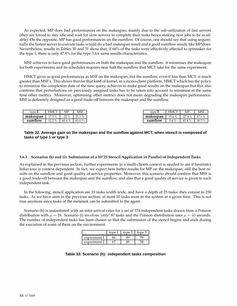
As expected, MP does bad performances on the makespan, mainly due to the sub-utilization of fast servers(they are forced to stay idle and wait for slow servers to complete their tasks hence making new jobs to be avail-able). On the opposite, MP has good performances on the sumflow. Of course, one should say that using sequen-tially the fastest server to execute tasks would do a bad makespan result and a good sumflow result, like MP does.Nevertheless, results in Tables 30 and 31 show that, if 66% of the tasks were effectively affected to spinnaker forthe type 1, there is only 47.8% for the type 3 for same results characteristics.
MSF achieves to have good performances on both the makespan and the sumflow: it minimises the makespanfor both experiments and its schedules requires near half the sumflow that MCT take for the same experiment.
HMCT gives as good preformances as MSF on the makespan, but the sumflow, even if less than MCT, is muchgreater than MSF’s. This shows that for that kind of kernel, in a mono-client platform, HMCT which has the policyto minimize the completion date of the new query, achieves to make good results on the makespan but this alsoconfirms that perturbations on previously assigned tasks has to be taken into account to minimise at the sametime other metrics. Moreover, optimising other metrics does not mean degrading the makespan performance:MSF is definetely designed as a good trade-off between the makespan and the sumflow.
type 1 HMCT MP MSFmakespan 17.3 % -22 % 21.1 %sumflow 12.2 % 60.6 % 41.6 %
type 3 HMCT MP MSFmakespan 15.6 % -27.4 % 17.1 %sumflow 5.6 % 47.4 % 30.7 %
Table 32. Average gain on the makespan and the sumflow against MCT, when stencil is composed oftasks of type 1 or type 3
5.6.3 Scenarios (h) and (i): Submission of a 10*25 Stencil Application in Parallel of Independent Tasks
As explained in the previous section, further experiments in a multi-clients context is needed to see if heuristicsbehaviour is context dependent. In fact, we expect here better results for MP on the makespan, still the best re-sults on the sumflow and good quality of service properties. Moreover, this scenario should confirm that MSF isa good trade-off between the makespan and the sumflow, and also that a good quality of service is given to eachindependent task.
In the folowing, stencil application are 10 tasks width wide, and have a depth of 25 tasks: they consist in 250tasks. As we have seen in the previous section, at most 10 tasks were in the system at a given time. This is nottrue anymore since tasks of the metatask can be submitted to the agent.
Scenario (h) is instantiated with an inter-arrival rates for a set of 174 independent tasks drawn from a Poissondistribution with µ = 28. Scenario (i) involves ‘only’ 87 tasks and the Poisson distribution uses µ = 45 seconds.The number of independent tasks has been chosen so that the submission of the stencil begins and ends duringthe execution of some of them on the environment.
type 1 type 2 type 3experiment 1 66 49 59experiment 2 67 49 58
Table 33. Scenario (h): independent tasks composition
RR n° 5168

Scenario (h)We have conducted two experiments of three runs each. One experiment consists in the submission of 174 inde-pendent tasks, whose detailed composition is given in Table 5.6.3, and a 10*25 stencil application. In consequence,424 tasks are submitted to the agent by two clients in a run.
The two experiments are generated with two different seeds to draw the arrival date of tasks of the indepen-dent tasks set and its composition. Then, even if the two sets have nearly the same composition (see Table 33), theorder and arrival dates are different). The difference between two arrival dates is drawn from a Poisson distribu-tion of mean equal here to µ = 28 seconds, and a task has a Uniform probability to be of one task type.
One should be coutious when reading HMCT results: during the first experiment, some independent taskshave not been accepted by servers (tasks 35 and 53, 38 and 49, and 37 in respectively the first, second and thirdrun). Moreover, in the second experiment, task 40 has been rejected in the first run. In the second run, task 48 andthe 48th submitted task of the stencil have not been processed. In the third run, the 46th and 71th submitted taskof the stencil have also been rejected. One must note that when a task is rejected by the environment, the task isconsidered as ‘done’ with a slightly nul duration. For independent tasks, this leads to an experiment with a lowerresource consumption in regard to the other heuristics. But for a task involved in a stencil, that also means thatsome tasks may be in a ready state before time.
Nonetheless, to have an idea of the HMCT results, we have used MCT results for the missing independenttasks and assumed that a missing stencil task have been mapped on spinnaker. HMCT is not able to handle thethroughput of this scenario at a high rate, but comparisons between MP, MSF and MCT are of course valid.
Average makespan and sumflow (with their respective standard deviation) of submitted applications graphsare presented in Figures 23 and 24. Detailed server utilization can be found in Table 34. Tables 35, 41 and 36contains respectively applications makespan and sumflow gains, results on different metrics for the independenttasks and average percentage per task gains.
0
500
1000
1500
2000
2500
3000
3500
4000
4500
5000
10 task set
time
(sec
)
client number
MCT
HMCT
MP
MSF
0
5000
10000
15000
20000
25000
30000
35000
10 task set
time
(sec
)
client number
MCT
HMCT
MP
MSF
Figure 23. Scenario (h): makespan and sumflow results for the first experiment
Results for HMCT are good and in one way the best we ever had in all the experiments, because for the firsttime it beats MSF on one metric: the makespan. But, as said previoulsy, some tasks are missing for being rejectedby a server that could not undertake it because of a too high load. Consequently these tasks have not interferedwith previoulsy and future assigned tasks on the corresponding server. Worst, the submission of the stencil isbiased, so the makespan. HMCT results can be seen as ‘ boosted up’.
We already encounter this situation during dgemm experiment (see section 5.2.1), with both MCT and HMCTheuristics. One must consider that HMCT tries to optimize MCT with the help of HTM information. Indeed,when the agent receives a new query, MCT computes its completion date as if no task would finish during itsexecution. This can be considered as a ‘worst case expectation’, because tasks can end up, minimizing the newquery completion date. HMCT tries to use the server capacity which is not able to accept another request. We donot have mechanisms to limit the number of tasks on a server, which could temperate the ‘aggressive’ behavior of
INRIA

0
500
1000
1500
2000
2500
3000
3500
4000
4500
5000
10 task set
time
(sec
)
client number
MCT
HMCT
MP
MSF
0
5000
10000
15000
20000
25000
30000
35000
10 task set
time
(sec
)
client number
MCT
HMCT
MP
MSF
Figure 24. Scenario (h): makespan and sumflow results for the second experiment
experiment 1server MCT HMCT MP MSF
% of tasks sumflow % of tasks sumflow % of tasks sumflow % of tasks sumflowspinnaker 49.1 (32.6 7.1 9.4) 28686 49.4 (33.8 7.3 8.3) 20656 50.7 (37.9 6.1 6.7) 15156 48.7 (33.5 7.3 7.9) 17467artimon 48.0 (40.3 3.7 4.0) 29052 40.3 (30.3 4.2 5.8) 23460 40.1 (30.4 4.3 5.3) 13735 39.4 (29.1 4.0 6.3) 15904soyotte 1.6 (0.8 0.4 0.4) 2183 5.0 (4.9 0.0 0.1) 2951 4.6 (3.3 0.5 0.9) 5896 5.8 (5.7 0.1 0.0) 4046fonck 1.4 (0.6 0.4 0.4) 1890 5.3 (5.3 0.0 0.0) 3179 4.6 (2.7 0.6 1.3) 6475 6.1 (6.0 0.2 0.0) 4462
total sumflow 61811 50246 41262 41879experiment 2
server MCT HMCT MP MSF% of tasks sumflow % of tasks sumflow % of tasks sumflow % of tasks sumflow
spinnaker 48.7 (33.3 6.7 8.7) 27258 48.8 (34.3 5.7 8.8) 18765 50.6 (38.0 5.4 7.2) 15337 47.4 (32.4 6.7 8.3) 17437artimon 48.6 (39.7 4.2 4.6) 30012 40.9 (30.0 5.8 5.1) 22099 41.4 (31.4 5.3 4.7) 14384 40.4 (30.0 4.8 5.6) 15988soyotte 1.0 (0.6 0.2 0.2) 1516 4.7 (4.7 0.0 0.0) 2757 4.0 (2.7 0.4 0.9) 5048 6.1 (6.1 0.0 0.0) 4299fonck 1.7 (0.9 0.5 0.3) 2364 5.6 (5.6 0.0 0.0) 3265 3.9 (2.4 0.5 1.0) 5566 6.1 (6.0 0.1 0.0) 4409
total sumflow 61150 46886 40335 42133MEAN
server MCT HMCT MP MSF% of tasks sumflow % of tasks sumflow % of tasks sumflow % of tasks sumflow
spinnaker 48.9 (33.0 6.9 9.0) 27972 49.1 (34.0 6.5 8.5) 19710 50.7 (37.9 5.8 7.0) 15246 48.0 (32.9 7.0 8.1) 17452artimon 48.3 (40.0 4.0 4.3) 29532 40.6 (30.1 5.0 5.5) 22780 40.8 (30.9 4.8 5.0) 14060 39.9 (29.6 4.4 5.9) 15946soyotte 1.3 (0.7 0.3 0.3) 1850 4.8 (4.8 0.0 0.0) 2854 4.3 (3.0 0.4 0.9) 5472 6.0 (5.9 0.0 0.0) 4172fonck 1.5 (0.7 0.4 0.4) 2127 5.5 (5.5 0.0 0.0) 3222 4.2 (2.6 0.6 1.1) 6020 6.1 (6.0 0.1 0.0) 4436
total sumflow 61480 48566 40798 42006
Table 34. Scenario (h): servers utilization
STENCILmakespan sumflow
HMCT MP MSF HMCT MP MSFexperiment 1 10.2 7.9 8.7 14.7 36.3 26.7experiment 2 8.5 6.0 8.2 20.4 36.2 26.9
MEAN 9.4 6.9 8.4 17.6 36.2 26.8
METATASKsumflow
HMCT MP MSF22.8 30.1 3825.5 31.4 36.224.2 30.8 37.1
Table 35. Scenario (h): average percentage gain against MCT on the makespan and the sumflow foreach client
HMCT, nor fault tolerance mechanisms (a client message would be needed to return the server ID to the agent),so the request is abandonned by the client.
RR n° 5168

mean flow gain in percentageMCT (sec) HMCT MP MSF
type 1 87.6 14.5 29.3 25.1experiment 1 type 2 163.0 22.8 28.7 38.0
type 3 279.1 25.6 31.1 42.4type 1 86.0 21.1 37.1 17.1
experiment 2 type 2 187.8 22.5 34.5 36.1type 3 250.0 31.0 28.1 42.3
MEAN - 175.6 22.9 31.5 33.5
Table 36. Scenario (h): average percentage gain for µ = 28 sec on each task given by type
Nonetheless, it is interesting to see that, even with this “time advantage”, MP and MSF are still beating HMCTon most of the metric on the average: this seems to confirm that minimizing the finishing completion time of thenew query without taking in account the interference with already assigned tasks is maybe not the right policy toundertake in our context.
We must also observe that MP does not give bad results on the makespan of the stencil application. Indeed,it even achieves a 7% gain. Because of independent tasks, we have not the ‘synchronization barier’ effect like inprevious scenarios.
Scenario (i)This section deals with the same kind of experiment as the one above. Inter-arrival date is drawn from a Poissondistribution with the parameter µ equal here to 40 seconds. 4 seeds have been used to generate the experimentswhose compositions are given in Table 37. Each of them have been submitted 6 times.
There are 86 independent tasks launched during the submission of a stencil application. The stencil graph is10 tasks wide width and 25 depth long. In consequence 336 tasks are submitted to the agent during a run.
type 1 type 2 type 3experiment 1 35 19 32experiment 2 30 24 32experiment 3 34 28 24experiment 4 28 28 30
Table 37. Scenario (i): independent tasks composition
One can see in Figures 25, 26, 27 and 28 graphs of the mean and standard deviation of the makespan andthe sumflow for stencil and metatask applications. Table 38 presents the cost per server in term of sumflow, thetotal sumflow cost of the experimentand tasks affectation percentages per server. In Table 39 gains realized onthe makespan and on the sumflow for the each client (here the client for the stencil and the client for the set ofindependent tasks) is given, and finally results on all metrics and quality of service for the independent tasks canbe found in Tables 40 and 42.
Firstly, one can observe that we obtain indentical results regardless the figure. On the makespan of the stencil,MSF is the best with a slight advance in front of MP and HMCT. On the sumflow, MP and MSF outperfom theother, MP with a higher standard deviation for the independent tasks and MSF for the stencil graph. Results havethen to decide between them.
Table 38 shows a that all heuristics behaves like they are used to unlike with scenarios (f) and (g).
INRIA
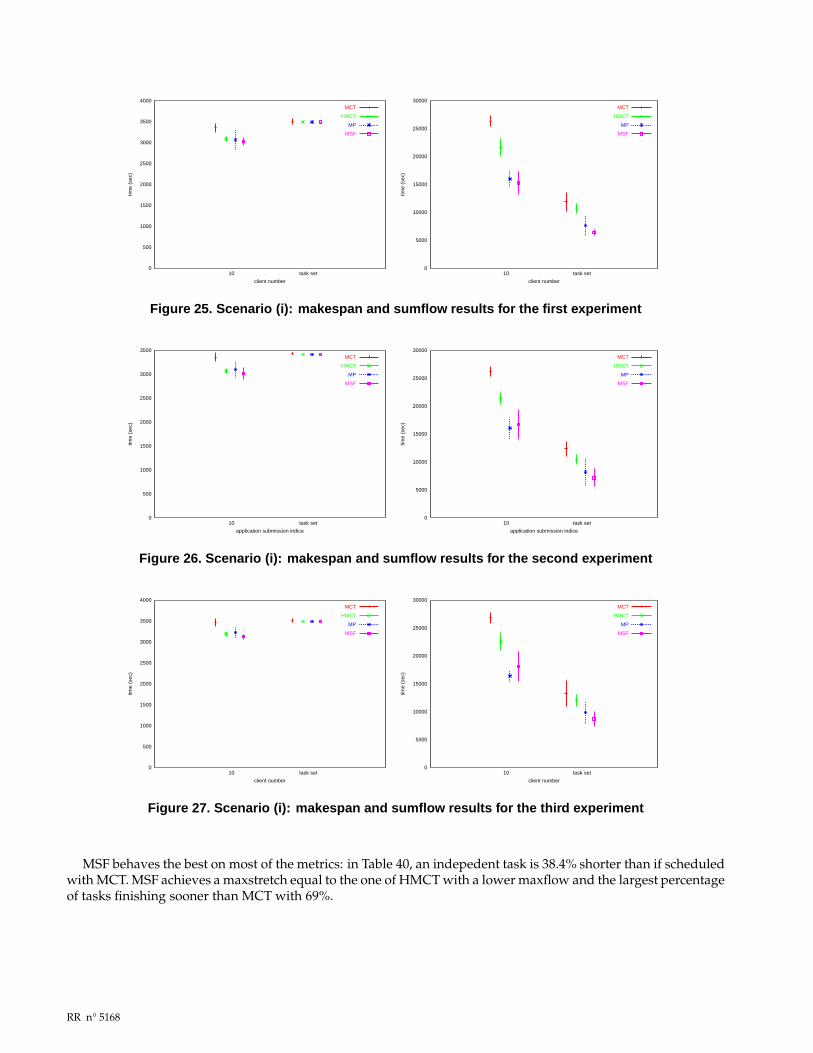
0
500
1000
1500
2000
2500
3000
3500
4000
10 task set
time
(sec
)
client number
MCT
HMCT
MP
MSF
0
5000
10000
15000
20000
25000
30000
10 task set
time
(sec
)
client number
MCT
HMCT
MP
MSF
Figure 25. Scenario (i): makespan and sumflow results for the first experiment
0
500
1000
1500
2000
2500
3000
3500
10 task set
time
(sec
)
application submission indice
MCT
HMCT
MP
MSF
0
5000
10000
15000
20000
25000
30000
10 task set
time
(sec
)
application submission indice
MCT
HMCT
MP
MSF
Figure 26. Scenario (i): makespan and sumflow results for the second experiment
0
500
1000
1500
2000
2500
3000
3500
4000
10 task set
time
(sec
)
client number
MCT
HMCT
MP
MSF
0
5000
10000
15000
20000
25000
30000
10 task set
time
(sec
)
client number
MCT
HMCT
MP
MSF
Figure 27. Scenario (i): makespan and sumflow results for the third experiment
MSF behaves the best on most of the metrics: in Table 40, an indepedent task is 38.4% shorter than if scheduledwith MCT. MSF achieves a maxstretch equal to the one of HMCT with a lower maxflow and the largest percentageof tasks finishing sooner than MCT with 69%.
RR n° 5168
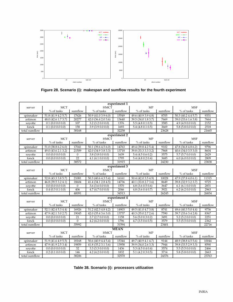
0
500
1000
1500
2000
2500
3000
3500
10 task set
time
(sec
)
client number
MCT
HMCT
MP
MSF
0
5000
10000
15000
20000
25000
30000
10 task set
time
(sec
)
client number
MCT
HMCT
MP
MSF
Figure 28. Scenario (i): makespan and sumflow results for the fourth experiment
experiment 1server MCT HMCT MP MSF
% of tasks sumflow % of tasks sumflow % of tasks sumflow % of tasks sumflowspinnaker 51.8 (41.9 4.2 5.7) 17626 50.9 (41.0 3.9 6.0) 15549 49.6 (40.9 3.9 4.8) 8705 50.3 (40.2 4.4 5.7) 9331artimon 48.0 (42.6 1.7 3.7) 20277 42.0 (36.4 2.0 3.6) 13640 39.5 (34.0 1.8 3.7) 7669 39.0 (33.6 1.6 3.8) 7664soyotte 0.1 (0.0 0.0 0.0) 107 3.2 (3.2 0.0 0.0) 1376 5.5 (4.8 0.1 0.5) 3585 4.9 (4.9 0.0 0.0) 2152fonck 0.1 (0.0 0.0 0.0) 158 3.9 (3.9 0.0 0.0) 1693 5.4 (4.8 0.1 0.5) 3669 5.8 (5.8 0.0 0.0) 2518
total sumflow 38168 32258 23628 21665experiment 2
server MCT HMCT MP MSF% of tasks sumflow % of tasks sumflow % of tasks sumflow % of tasks sumflow
spinnaker 51.0 (38.8 6.2 6.0) 17041 50.1 (39.6 4.5 6.0) 14763 49.4 (39.8 4.2 5.4) 9102 47.8 (36.8 4.8 6.2) 9796artimon 49.0 (43.6 2.1 3.2) 21509 42.0 (34.9 3.8 3.3) 13718 39.8 (33.3 3.3 3.2) 7868 40.6 (34.0 3.5 3.0) 8604soyotte 0.0 (0.0 0.0 0.0) 0 3.8 (3.8 0.0 0.0) 1639 5.4 (4.5 0.6 0.2) 3575 5.7 (5.7 0.0 0.0) 2629fonck 0.0 (0.0 0.0 0.0) 22 4.1 (4.1 0.0 0.0) 1795 5.4 (4.8 0.2 0.4) 3685 6.0 (6.0 0.0 0.0) 2809
total sumflow 38572 31915 24230 23838experiment 3
server MCT HMCT MP MSF% of tasks sumflow % of tasks sumflow % of tasks sumflow % of tasks sumflow
spinnaker 52.8 (43.3 3.8 5.7) 21081 50.3 (40.6 4.3 5.4) 16161 50.4 (42.0 3.5 4.9) 10028 47.9 (37.8 4.0 6.1) 11315artimon 46.8 (39.5 3.2 4.1) 18604 41.4 (34.1 2.8 4.5) 14736 40.1 (33.8 2.7 3.6) 8649 39.8 (32.9 3.2 3.7) 9725soyotte 0.0 (0.0 0.0 0.0) 0 3.6 (3.6 0.0 0.0) 1570 4.8 (3.6 0.5 0.6) 3647 6.1 (6.1 0.0 0.0) 2831fonck 0.4 (0.3 0.1 0.0) 406 4.7 (4.7 0.0 0.0) 2046 4.8 (3.6 0.4 0.7) 3921 6.2 (6.2 0.0 0.0) 2963
total sumflow 40091 34513 26245 26834experiment 4
server MCT HMCT MP MSF% of tasks sumflow % of tasks sumflow % of tasks sumflow % of tasks sumflow
spinnaker 52.1 (42.4 5.3 4.4) 16926 51.2 (42.3 4.8 4.2) 14903 49.5 (41.0 4.7 3.8) 8741 49.6 (40.3 5.0 4.4) 9736artimon 47.9 (42.1 3.0 2.7) 19045 42.0 (35.4 3.6 3.0) 13737 40.3 (35.0 2.7 2.6) 7590 39.7 (33.6 3.4 2.8) 8367soyotte 0.0 (0.0 0.0 0.0) 21 2.7 (2.7 0.0 0.0) 1158 5.6 (5.0 0.3 0.2) 3491 5.2 (5.2 0.0 0.0) 2251fonck 0.0 (0.0 0.0 0.0) 0 4.2 (4.2 0.0 0.0) 1796 4.7 (3.5 0.6 0.5) 3579 5.5 (5.5 0.0 0.0) 2362
total sumflow 35992 31594 23401 22716MEAN
server MCT HMCT MP MSF% of tasks sumflow % of tasks sumflow % of tasks sumflow % of tasks sumflow
spinnaker 51.9 (41.6 4.9 5.5) 18168 50.6 (40.9 4.4 5.4) 15344 49.7 (40.9 4.1 4.7) 9144 48.9 (38.8 4.5 5.6) 10044artimon 47.9 (41.9 2.5 3.4) 19859 41.8 (35.2 3.1 3.6) 13958 39.9 (34.0 2.6 3.3) 7944 39.8 (33.5 2.9 3.3) 8590soyotte 0.0 (0.0 0.0 0.0) 32 3.3 (3.3 0.0 0.0) 1436 5.3 (4.5 0.4 0.4) 3574 5.5 (5.5 0.0 0.0) 2466fonck 0.2 (0.1 0.0 0.0) 146 4.2 (4.2 0.0 0.0) 1832 5.1 (4.2 0.3 0.5) 3714 5.8 (5.8 0.0 0.0) 2663
total sumflow 38206 32570 24376 23763
Table 38. Scenario (i): processors utilization
INRIA
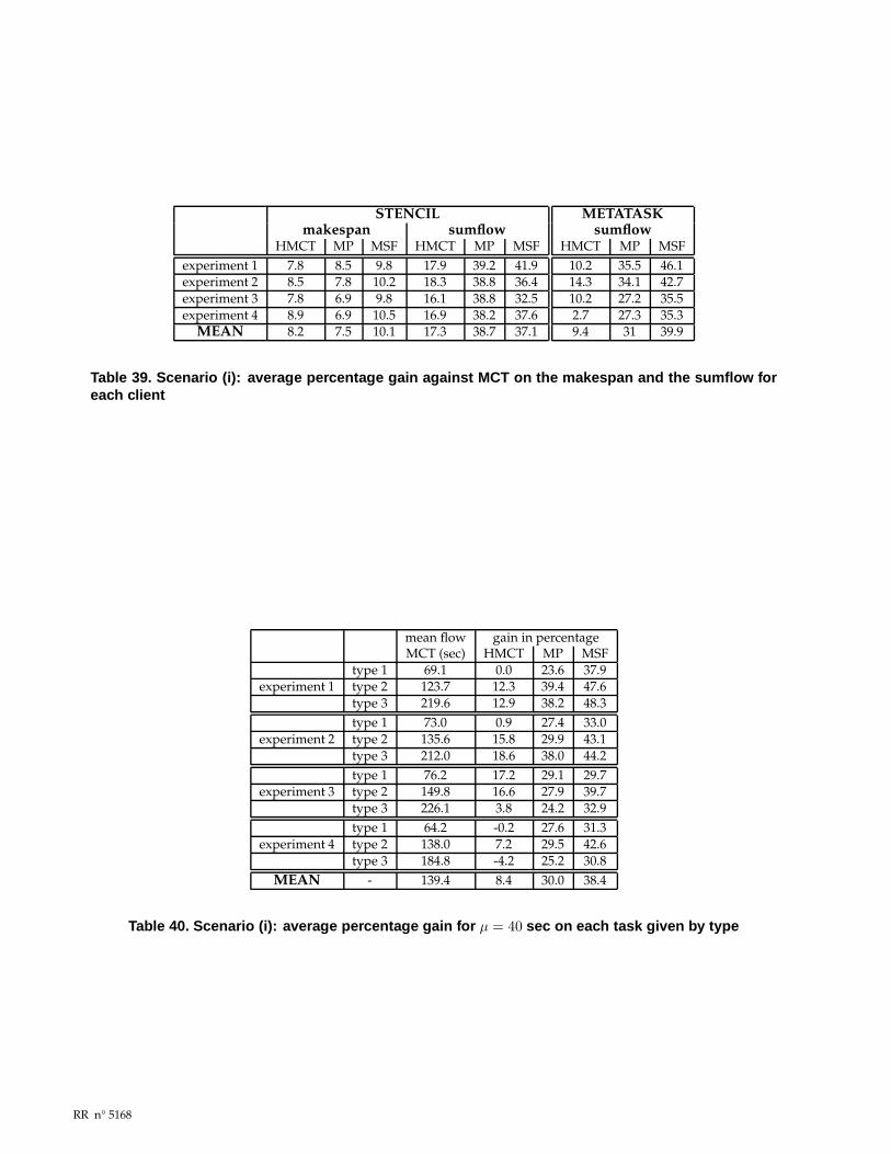
STENCILmakespan sumflow
HMCT MP MSF HMCT MP MSFexperiment 1 7.8 8.5 9.8 17.9 39.2 41.9experiment 2 8.5 7.8 10.2 18.3 38.8 36.4experiment 3 7.8 6.9 9.8 16.1 38.8 32.5experiment 4 8.9 6.9 10.5 16.9 38.2 37.6
MEAN 8.2 7.5 10.1 17.3 38.7 37.1
METATASKsumflow
HMCT MP MSF10.2 35.5 46.114.3 34.1 42.710.2 27.2 35.52.7 27.3 35.39.4 31 39.9
Table 39. Scenario (i): average percentage gain against MCT on the makespan and the sumflow foreach client
mean flow gain in percentageMCT (sec) HMCT MP MSF
type 1 69.1 0.0 23.6 37.9experiment 1 type 2 123.7 12.3 39.4 47.6
type 3 219.6 12.9 38.2 48.3type 1 73.0 0.9 27.4 33.0
experiment 2 type 2 135.6 15.8 29.9 43.1type 3 212.0 18.6 38.0 44.2type 1 76.2 17.2 29.1 29.7
experiment 3 type 2 149.8 16.6 27.9 39.7type 3 226.1 3.8 24.2 32.9type 1 64.2 -0.2 27.6 31.3
experiment 4 type 2 138.0 7.2 29.5 42.6type 3 184.8 -4.2 25.2 30.8
MEAN - 139.4 8.4 30.0 38.4
Table 40. Scenario (i): average percentage gain for µ = 40 sec on each task given by type
RR n° 5168

NetSolve’s MCT HMCT MP MSFseed1 seed2 Avg seed1 seed2 Avg seed1 seed2 Avg seed1 seed2 Avg
makespan 4911 4835 4873 4915 4839 4877 4911 4839 4875 4917 4839 4878
sumflow 30426 29625 30026 23485 21793 22639 21254 20209 20732 18863 19092 18978
maxflow 575.5 637.6 606.5 399.1 419.9 409.5 658.0 608.4 633.2 310.7 344.1 327.4
maxstretch 19.3 21.8 20.6 10.8 10.9 10.8 19.0 17.7 18.3 15.9 14.7 15.3
percentage oftasks that finish - - − 61 (30) 61 (26) 61(28) 69 (19) 70 (17) 70(18) 75 (16) 66 (21) 70(18)
sooner than withNetSolve’s MCT
Table 41. Scenario (h): results in seconds for µ = 28 sec on wastecpu tasksNetSolve’s MCT HMCT MP MSF
seed1 seed2 seed3 seed4 Avg seed1 seed2 seed3 seed4 Avg seed1 seed2 seed3 seed4 Avg seed1 seed2 seed3 seed4 Avg
makespan 3504 3437 3505 3464 3478 3489 3415 3480 3462 3462 3489 3415 3480 3462 3462 3489 3415 3480 3462 3462
sumflow 11853 12341 13270 10482 11986 10643 10496 12012 10392 10886 7640 8167 9819 7623 8312 6387 7146 8726 6788 7262
maxflow 405.5 429.7 401.2 415.1 412.9 317.3 286.8 337.8 325.9 316.9 463.0 468.7 482.4 457.0 467.8 199.3 220.1 274.0 237.7 232.8
maxstretch 10.7 10.4 10.1 10.1 10.3 8.3 9.5 8.4 8.6 8.7 14.3 13.3 14.2 13.2 13.8 6.7 9.3 10.8 8.3 8.8
percentageof tasks - - - - − 52 (40) 56 (37) 54 (39) 49 (41) 53(39) 67 (25) 69 (25) 67 (26) 60 (30) 66(26) 71 (21) 74 (20) 68 (25) 62 (29) 69(24)
that finishsooner thanwith MCT
Table 42. Scenario (i): results in seconds for µ = 40 sec on wastecpu tasks
INR
IA

5.7. Scenario (j): Submission of a 5*25 Stencil Application Concurrently to 87 Independent Tasks at a LowRate
We consider the submission of a 5*25 stencil application in parallel of 86 independent tasks. The syencil graphis composed of task of type 1 and its width is smaller than in previous scenarios in order to judge the heuristicsfacing a lower throughput.
Indeed, the inter-arrival date of two independent tasks is drawn from a Poisson distribution with parameterµ = 25 seconds and only 5 tasks are submitted at the beginning of the stencil submission.
Four seeds have been used to generate four instantiations of this scenario. Each of them have been submitted6 times to the environment composed of the following servers:
• client: zanzibar ;
• agent: xrousse ;
• servers: spinnaker, artimon, soyotte, fonck.
0
500
1000
1500
2000
2500
3000
3500
1 task set
time
(sec
)
client number
MCT
HMCT
MP
MSF
0
2000
4000
6000
8000
10000
12000
14000
1 task set
time
(sec
)
client number
MCT
HMCT
MP
MSF
Figure 29. Scenario (j): makespan and sumflow results for the first experiment
0
500
1000
1500
2000
2500
3000
1 task set
time
(sec
)
client number
MCT
HMCT
MP
MSF
0
2000
4000
6000
8000
10000
12000
14000
1 task set
time
(sec
)
client number
MCT
HMCT
MP
MSF
Figure 30. Scenario (j): makespan and sumflow results for the second experiment
Makespan and sumflow results are given in Figures 29, 30, 31 and 32. Servers utilization is given in Table 43and resulting gains are described in Table 44. Results on the response time is given in Table 45 and an overviewof the maxflow, maxtretch metrics as well as the percentage of tasks that finish sooner is provided in Table 46.
The first thing to point out is that MP does not achieve the same result on the makespan than in scenario (g)and (h): it gives the highest makespan, 33.8% higher than the one given by the MCT schedule for the stencil
RR n° 5168
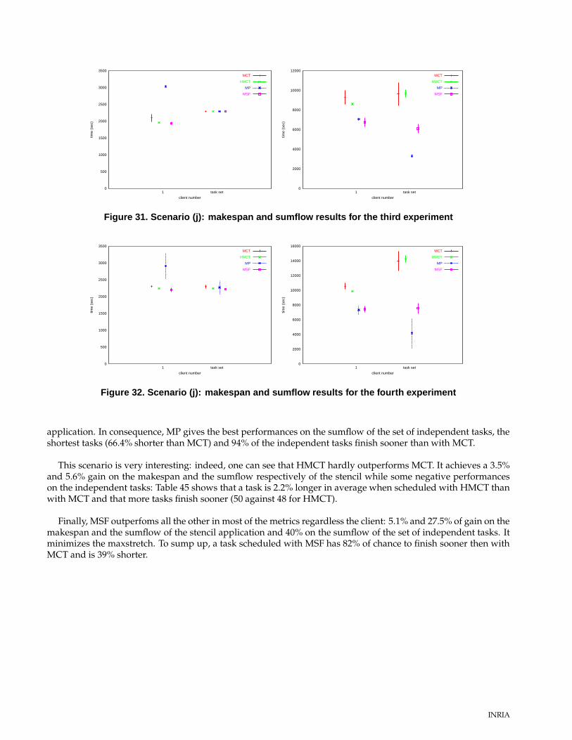
0
500
1000
1500
2000
2500
3000
3500
1 task set
time
(sec
)
client number
MCT
HMCT
MP
MSF
0
2000
4000
6000
8000
10000
12000
1 task set
time
(sec
)
client number
MCT
HMCT
MP
MSF
Figure 31. Scenario (j): makespan and sumflow results for the third experiment
0
500
1000
1500
2000
2500
3000
3500
1 task set
time
(sec
)
client number
MCT
HMCT
MP
MSF
0
2000
4000
6000
8000
10000
12000
14000
16000
1 task set
time
(sec
)
client number
MCT
HMCT
MP
MSF
Figure 32. Scenario (j): makespan and sumflow results for the fourth experiment
application. In consequence, MP gives the best performances on the sumflow of the set of independent tasks, theshortest tasks (66.4% shorter than MCT) and 94% of the independent tasks finish sooner than with MCT.
This scenario is very interesting: indeed, one can see that HMCT hardly outperforms MCT. It achieves a 3.5%and 5.6% gain on the makespan and the sumflow respectively of the stencil while some negative performanceson the independent tasks: Table 45 shows that a task is 2.2% longer in average when scheduled with HMCT thanwith MCT and that more tasks finish sooner (50 against 48 for HMCT).
Finally, MSF outperfoms all the other in most of the metrics regardless the client: 5.1% and 27.5% of gain on themakespan and the sumflow of the stencil application and 40% on the sumflow of the set of independent tasks. Itminimizes the maxstretch. To sump up, a task scheduled with MSF has 82% of chance to finish sooner then withMCT and is 39% shorter.
INRIA
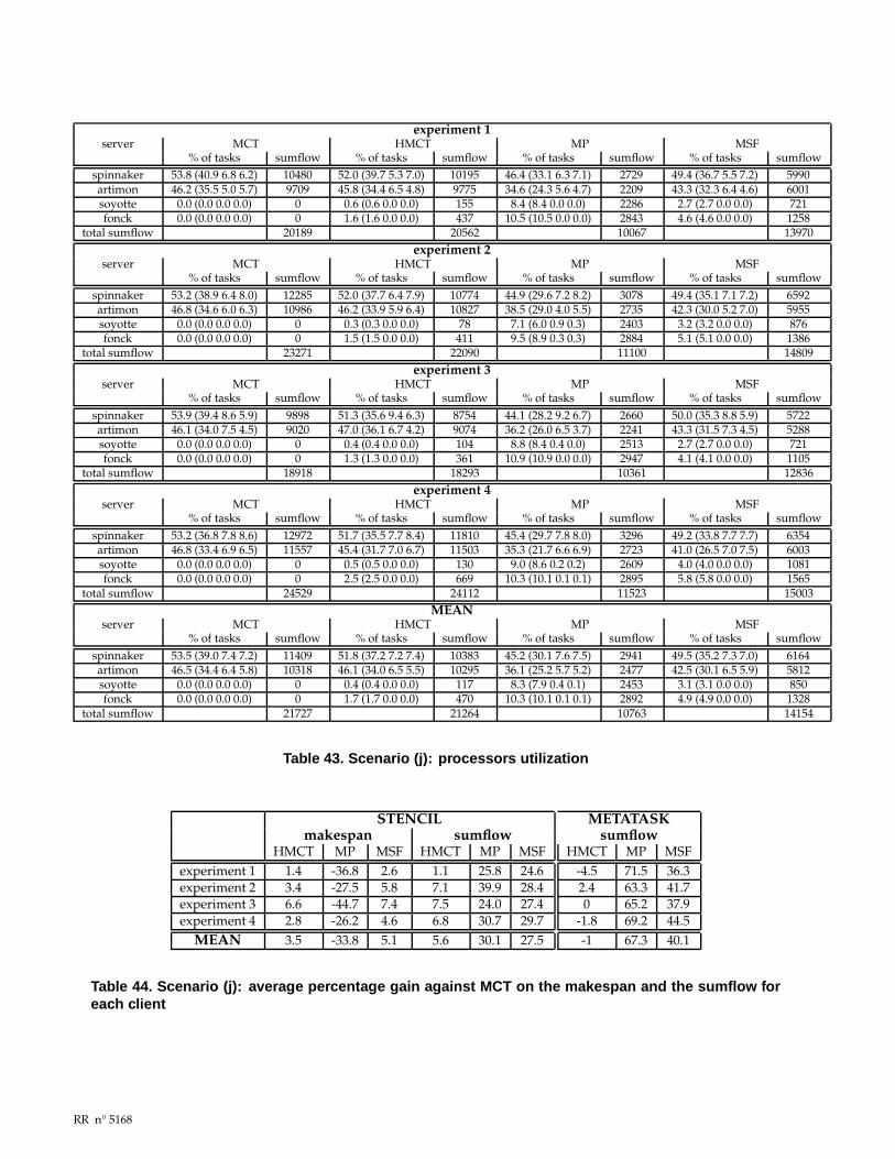
experiment 1server MCT HMCT MP MSF
% of tasks sumflow % of tasks sumflow % of tasks sumflow % of tasks sumflowspinnaker 53.8 (40.9 6.8 6.2) 10480 52.0 (39.7 5.3 7.0) 10195 46.4 (33.1 6.3 7.1) 2729 49.4 (36.7 5.5 7.2) 5990artimon 46.2 (35.5 5.0 5.7) 9709 45.8 (34.4 6.5 4.8) 9775 34.6 (24.3 5.6 4.7) 2209 43.3 (32.3 6.4 4.6) 6001soyotte 0.0 (0.0 0.0 0.0) 0 0.6 (0.6 0.0 0.0) 155 8.4 (8.4 0.0 0.0) 2286 2.7 (2.7 0.0 0.0) 721fonck 0.0 (0.0 0.0 0.0) 0 1.6 (1.6 0.0 0.0) 437 10.5 (10.5 0.0 0.0) 2843 4.6 (4.6 0.0 0.0) 1258
total sumflow 20189 20562 10067 13970experiment 2
server MCT HMCT MP MSF% of tasks sumflow % of tasks sumflow % of tasks sumflow % of tasks sumflow
spinnaker 53.2 (38.9 6.4 8.0) 12285 52.0 (37.7 6.4 7.9) 10774 44.9 (29.6 7.2 8.2) 3078 49.4 (35.1 7.1 7.2) 6592artimon 46.8 (34.6 6.0 6.3) 10986 46.2 (33.9 5.9 6.4) 10827 38.5 (29.0 4.0 5.5) 2735 42.3 (30.0 5.2 7.0) 5955soyotte 0.0 (0.0 0.0 0.0) 0 0.3 (0.3 0.0 0.0) 78 7.1 (6.0 0.9 0.3) 2403 3.2 (3.2 0.0 0.0) 876fonck 0.0 (0.0 0.0 0.0) 0 1.5 (1.5 0.0 0.0) 411 9.5 (8.9 0.3 0.3) 2884 5.1 (5.1 0.0 0.0) 1386
total sumflow 23271 22090 11100 14809experiment 3
server MCT HMCT MP MSF% of tasks sumflow % of tasks sumflow % of tasks sumflow % of tasks sumflow
spinnaker 53.9 (39.4 8.6 5.9) 9898 51.3 (35.6 9.4 6.3) 8754 44.1 (28.2 9.2 6.7) 2660 50.0 (35.3 8.8 5.9) 5722artimon 46.1 (34.0 7.5 4.5) 9020 47.0 (36.1 6.7 4.2) 9074 36.2 (26.0 6.5 3.7) 2241 43.3 (31.5 7.3 4.5) 5288soyotte 0.0 (0.0 0.0 0.0) 0 0.4 (0.4 0.0 0.0) 104 8.8 (8.4 0.4 0.0) 2513 2.7 (2.7 0.0 0.0) 721fonck 0.0 (0.0 0.0 0.0) 0 1.3 (1.3 0.0 0.0) 361 10.9 (10.9 0.0 0.0) 2947 4.1 (4.1 0.0 0.0) 1105
total sumflow 18918 18293 10361 12836experiment 4
server MCT HMCT MP MSF% of tasks sumflow % of tasks sumflow % of tasks sumflow % of tasks sumflow
spinnaker 53.2 (36.8 7.8 8.6) 12972 51.7 (35.5 7.7 8.4) 11810 45.4 (29.7 7.8 8.0) 3296 49.2 (33.8 7.7 7.7) 6354artimon 46.8 (33.4 6.9 6.5) 11557 45.4 (31.7 7.0 6.7) 11503 35.3 (21.7 6.6 6.9) 2723 41.0 (26.5 7.0 7.5) 6003soyotte 0.0 (0.0 0.0 0.0) 0 0.5 (0.5 0.0 0.0) 130 9.0 (8.6 0.2 0.2) 2609 4.0 (4.0 0.0 0.0) 1081fonck 0.0 (0.0 0.0 0.0) 0 2.5 (2.5 0.0 0.0) 669 10.3 (10.1 0.1 0.1) 2895 5.8 (5.8 0.0 0.0) 1565
total sumflow 24529 24112 11523 15003MEAN
server MCT HMCT MP MSF% of tasks sumflow % of tasks sumflow % of tasks sumflow % of tasks sumflow
spinnaker 53.5 (39.0 7.4 7.2) 11409 51.8 (37.2 7.2 7.4) 10383 45.2 (30.1 7.6 7.5) 2941 49.5 (35.2 7.3 7.0) 6164artimon 46.5 (34.4 6.4 5.8) 10318 46.1 (34.0 6.5 5.5) 10295 36.1 (25.2 5.7 5.2) 2477 42.5 (30.1 6.5 5.9) 5812soyotte 0.0 (0.0 0.0 0.0) 0 0.4 (0.4 0.0 0.0) 117 8.3 (7.9 0.4 0.1) 2453 3.1 (3.1 0.0 0.0) 850fonck 0.0 (0.0 0.0 0.0) 0 1.7 (1.7 0.0 0.0) 470 10.3 (10.1 0.1 0.1) 2892 4.9 (4.9 0.0 0.0) 1328
total sumflow 21727 21264 10763 14154
Table 43. Scenario (j): processors utilization
STENCILmakespan sumflow
HMCT MP MSF HMCT MP MSFexperiment 1 1.4 -36.8 2.6 1.1 25.8 24.6experiment 2 3.4 -27.5 5.8 7.1 39.9 28.4experiment 3 6.6 -44.7 7.4 7.5 24.0 27.4experiment 4 2.8 -26.2 4.6 6.8 30.7 29.7
MEAN 3.5 -33.8 5.1 5.6 30.1 27.5
METATASKsumflow
HMCT MP MSF-4.5 71.5 36.32.4 63.3 41.70 65.2 37.9
-1.8 69.2 44.5-1 67.3 40.1
Table 44. Scenario (j): average percentage gain against MCT on the makespan and the sumflow foreach client
RR n° 5168
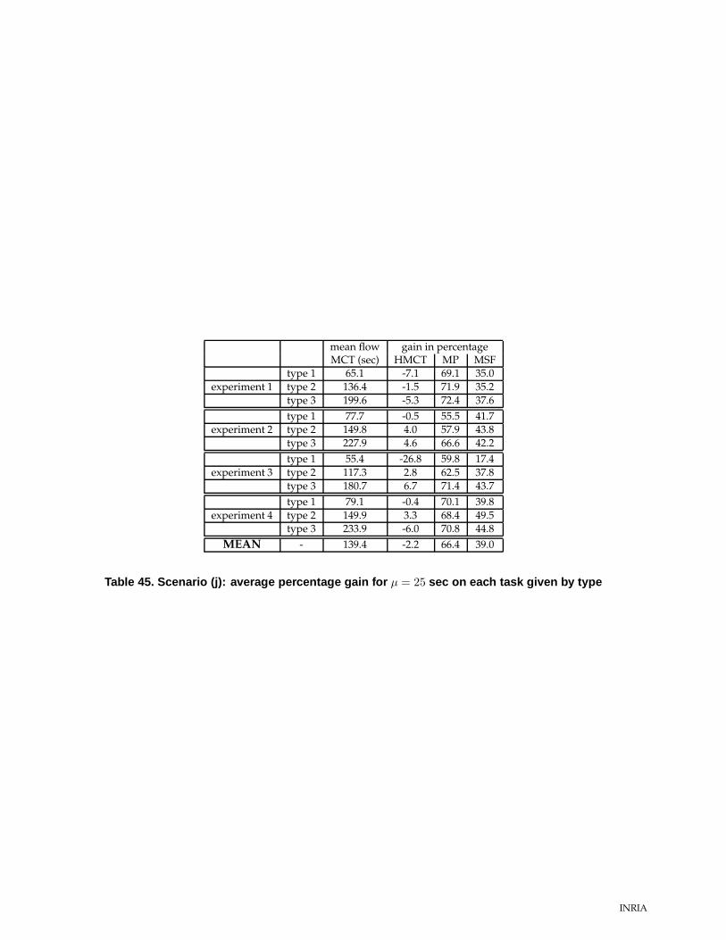
mean flow gain in percentageMCT (sec) HMCT MP MSF
type 1 65.1 -7.1 69.1 35.0experiment 1 type 2 136.4 -1.5 71.9 35.2
type 3 199.6 -5.3 72.4 37.6type 1 77.7 -0.5 55.5 41.7
experiment 2 type 2 149.8 4.0 57.9 43.8type 3 227.9 4.6 66.6 42.2type 1 55.4 -26.8 59.8 17.4
experiment 3 type 2 117.3 2.8 62.5 37.8type 3 180.7 6.7 71.4 43.7type 1 79.1 -0.4 70.1 39.8
experiment 4 type 2 149.9 3.3 68.4 49.5type 3 233.9 -6.0 70.8 44.8
MEAN - 139.4 -2.2 66.4 39.0
Table 45. Scenario (j): average percentage gain for µ = 25 sec on each task given by type
INRIA
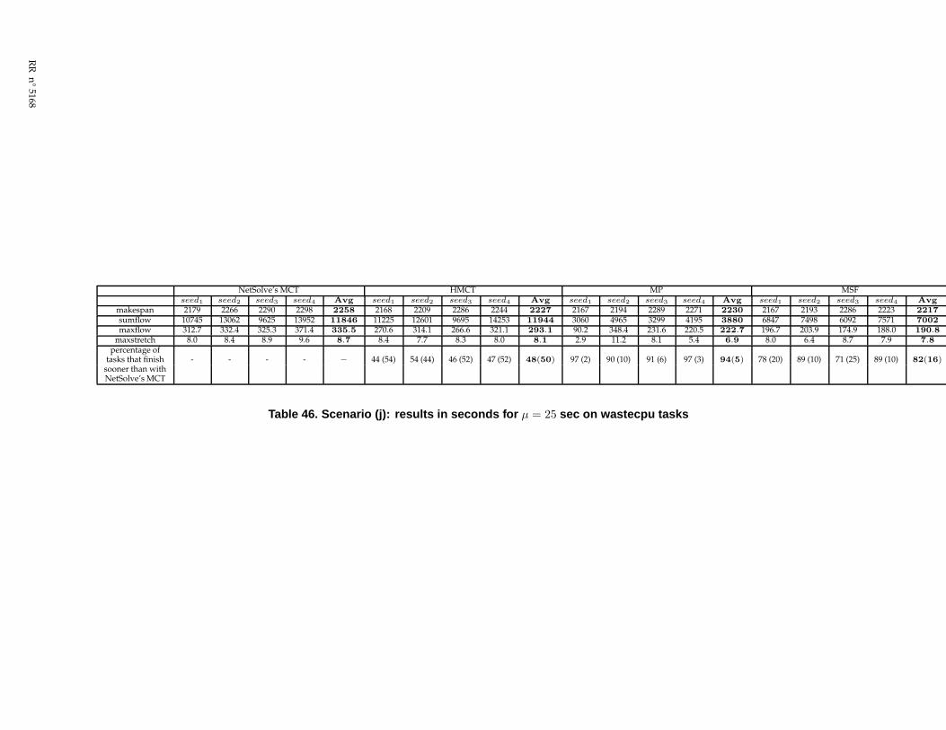
NetSolve’s MCT HMCT MP MSFseed1 seed2 seed3 seed4 Avg seed1 seed2 seed3 seed4 Avg seed1 seed2 seed3 seed4 Avg seed1 seed2 seed3 seed4 Avg
makespan 2179 2266 2290 2298 2258 2168 2209 2286 2244 2227 2167 2194 2289 2271 2230 2167 2193 2286 2223 2217
sumflow 10745 13062 9625 13952 11846 11225 12601 9695 14253 11944 3060 4965 3299 4195 3880 6847 7498 6092 7571 7002
maxflow 312.7 332.4 325.3 371.4 335.5 270.6 314.1 266.6 321.1 293.1 90.2 348.4 231.6 220.5 222.7 196.7 203.9 174.9 188.0 190.8
maxstretch 8.0 8.4 8.9 9.6 8.7 8.4 7.7 8.3 8.0 8.1 2.9 11.2 8.1 5.4 6.9 8.0 6.4 8.7 7.9 7.8
percentage oftasks that finish - - - - − 44 (54) 54 (44) 46 (52) 47 (52) 48(50) 97 (2) 90 (10) 91 (6) 97 (3) 94(5) 78 (20) 89 (10) 71 (25) 89 (10) 82(16)
sooner than withNetSolve’s MCT
Table 46. Scenario (j): results in seconds for µ = 25 sec on wastecpu tasks
RR
n°5168

5.8. Notes on Heuristics
MCT is the heuristic used by default in NetSolve [CD96]. In fact, it is the only proposed heuristic because it isconsidered as one of the easiest to implement and one of the best on the makespan metric (note that in [MAS+99],they study it in a space-share context).We use in this work a platform that has an heterogeneity coefficient (Section 5.1) of at least 6, but 8.9 in the ma-jority of the experiments exposed. On the platform corresponding to this last coefficient, e.g. spinnaker, artimon,fonck and soyotte (Table 3), MCT never really uses the 2 slower servers by itself: when they are used, then, forthe main part, it is consequent of the reject of the submission by all overloaded servers that were sorted beforein the list given to the client. So it is only thankful to the client error management that MCT may face such anheterogeneity. Consequently, scheduling decisions have disastrous consequences on applications performancesas well as on system integrity.Other remarks are presented below, because they are common with HMCT behavior, and are even easier to ex-plain there.
Historical-MCT relies on both MCT policy and the Historical Trace Manager (Section 2.3). This heuristic can beseen as a ‘perfect’ time-share MCT, because it has a priori a more accurate information on the system state. We useit to judge the pertinence of the idea to minimize the completion time of the last submitted task as regard to theobserved metrics. Nevertheless, results show that this policy is not the best even in a mono-client environment(see Scenarios (f) and (g)) and not only on the makespan. Moreover, HMCT tends to overload a server whichleads to the incapacity to handle all the submissions in some scenarios.
HMCT is better than MCT, but is well outperformed compared against MP and MSF which have constantlygood results regardless the metric, the environment, the number of clients or tasks in the system.
MP uses only the perturbation to compute where to map a new request. Consequently it uses more the slowestservers for tasks of long duration because that kind of task generates more perturbations on a fast and loadedserver. On the opposite, MSF uses the simulated duration and then, as long tasks are even longer on slow servers,the schedule generally tends to use slow servers for shorter tasks. These behaviors are confirmed by the results.
MP is better with contention: it gives the best results when the submission throughput is really high for theenvironment. We have pointed out a drawback that has been showed with Scenarios (f) and (g) for mono-clientexperiments. As soon as independent tasks are also involved, it can disappear (Scenarios (h) and (i)) or turn to anadvantage on other metrics (Scenario (j)).
MSF achieves great performances regardless the metric or the scenario. It gives a good makespan to each client,and good quality of service to independent tasks. It mixes HMCT and MP advantages without their respectivedrawbacks.
6. Improvements and Future Work
One of the first improvement to implement is the task feedback. There is three ways doing so. Indeed, it canbe considered that the job to inform the agent is the server’s, or the client’s or both. If the last one is used, thennetwork measures can also be computed.
In current NetSolve code, servers send load reports and finishing task messages to the agent. Nevertheless weneed to know in our work which task has been terminated on the server. In order to know this, the agent mustassign a unique number to each task and this IDentification must be known by the agent of course, but also by theclient or both the client and the server.
At current time, this work is done and also used in NetSolve and in the VisPerf monitor 3 to have more preciseinformation. The HTM has to change some cost values and the adjustment is taken into account for the nextsubmission, during the scheduling decision, when it gives information to the heuristic.
The completion feedback let to consider:
3http://icl.cs.utk.edu/netsolvedev/applications/visperf.html
INRIA
• It can be used to store the exact duration of some determinist tasks that have been executed on the envi-ronment. This can next be used to compute an interpolation of the complexity polynomial, and then moreprecise expectations of the duration of that class of tasks ;
• The memory management may be a mean to forbid expensive swap exchanges (which are not taken intoaccount in our heuristics) and limit the number of jobs on a server. Nonetheless, this should not be seen as apalliative to the HMCT drawback, because like most of experiments show, servers may even collapse withonly computing intensive tasks ;
• Job Cancellation is not feasible in the current state of our work, but seems an a priori direct algorithm tocode ;
• Even if computing intensive tasks are intrusive in a user system, the heuristic has to manage non-dedicatedplatforms. For this work, information coming from the /proc directory on Unix server can also be helpful.
These improvements let us envisage other heuristics, some relying on a tradeoff between load and memory con-sumption.
Moreover, further works has to be done to implement the HTM and the heuristics in DIET [CDF+01], a frenchProblem Solving Environment built on top of a hierarchical agent structure.
7. Conclusions
We have examined the behavior of four heuristics Minimum Completion Time, Historical MCT, MinimumPerturbation and Minimum Sumflow facing numerous different scenarios of submission in real environments.Some scenarios, like Scenarios (a) and (b), involve only independent tasks. Others involve 1D-mesh or stencilapplications like Scenarios (c), (d), (f) et (g). Scenarios (e), (h), (i) and (j) mix the two kinds. The experimentations,if extensive, cannot be exhaustive: there are an infinity of possible variants that would require too many time.Our work already represents more than 50 days of non-stop running. Nonetheless, we believe that our results aresignificant to validate the HTM and our heuristics.
We have compared our heuristics HMCT, MP and MSF against MCT, a widely used scheduling heuristic andthe default in NetSolve, a Problem Solving Environment. They rely on a prediction module called the HistoricalTrace Manager. The HTM simulates the execution of all the tasks on the environment and give according informa-tion on the duration of any task that has been submitted. These information can be exploited to try to minimizeother metric than the common makespan at the same time.
For this work, the HTM and the heuristics have been integrated in the code of NetSolve. The distributed hetero-geneous servers used for our experiments were dedicated to the environment, but the network is the laboratory’s.
Our work shows that MCT, with load correction mechanisms, do not achieve to perform well in a time-shareenvironment of heterogeneity coefficient of at least 6. HMCT gives much better results in average. This validatesthe HTM approach because HMCT and MCT rely on the same policy: to finish the last request the soonest inorder to minimize the overall makespan.
Nevertheless locally optimizing the makespan may not be the best policy: tasks that have been scheduled forsome reason on a server can be delayed by future request(s). With the HTM information, heuristics can considerthe perturbation tasks have on each other. This have the two following consequences: a better accuracy on thesystem state and the possiblity to exploit at best the available resources for the new task without penalizing stillrunning tasks. This gives a higher quality of service to each client.
Results show that HMCT, MP and MSF, specifically designed for heterogeneous environment where there isa high probablity of perturbation, outperform MCT. MSF appears to be the best averall heuristics as it alwaysoutperforms MCT on all criteria.
RR n° 5168
References
[Bak74] K.R. Baker. Introduction to Sequencing and Scheduling. Wiley, 1974.
[BBR01] O. Beaumont, V. Boudet, and Y. Robert. The iso-level scheduling heuristic for heterogeneous proces-sors. Technical Report RR-2001-22, LIP, ENS Lyon, May 2001.
[BCM98] M.A. Bender, S. Chakrabarti, and S. Muthukrishnan. Flow and stretch metrics for scheduling contin-uous job streams. In SODA: ACM-SIAM Symposium on Discrete Algorithms, 1998.
[BSB+99] T.D. Braun, H.J. Siegel, N. Beck, L. Bölöni, M. Maheswaran, A.I. Reuther, J.P. Robertson, M.D. Theys,B. Yao, D.H., and Richard F. Freund. A comparison study of static mapping heuritsics for a class ofmeta-tasks on heterogeneous computing systems. In Proceedings of the 8th Heterogeneous ComputingWorkshop (HCW ’99), april 1999.
[Cas01] H. Casanova. Simgrid: A toolkit for the simulation of application scheduling. In Proceedings of theIEEE Symposium on Cluster Computing and the Grid (CCGrid’01). IEEE Computer Society, may 2001.available on http://www-cse.ucsd.edu/ casanova/.
[CD96] H. Casanova and J. Dongarra. Netsolve : A network server for solving computational science prob-lems. In Proceedings of Super-Computing -Pittsburg, 1996.
[CDF+01] E. Caron, F. Desprez, E. Fleury, D. Lombard, J.M. Nicod, M. Quinson, and F. Suter. Une approchehiérarchique des serveurs de calcul. to appear in Calculateurs Parallèles, numéro spécial metacomputing,2001. http://www.ens-lyon.fr/ desprez/DIET/index.htm.
[CJ02] Y. Caniou and E. Jeannot. Dynamic mapping of a metatask on the grid: Historical trace, minimumperturbation and minimum length heuristics. Technical Report 4620, LORIA, nancy, oct 2002.
[GW97] A.S. Grimshaw and W.A. Wulf. The legion vision of a worldwide virtual computer. Communicationsof the ACM, 40(1):39–45, 1997.
[MAS+99] M. Maheswaran, S. Ali, H.J. Siegel, D. Hengsen, and R.F. Freund. Dynamic matching and schedul-ing of a class of independent tasks onto heterogeneous computing system. In Proceedings of the 8thHeterogeneous Computing Workshop (HCW ’99), april 1999.
[NMS+03] H. Nakada, S. Matsuoka, K. Seymour, J. Dongarra, C. Lee, and H. Casanova.A GridRPC Model and API for End-User Applications, December 2003.https://forge.gridforum.org/projects/gridrpc-wg/document/GridRPC_EndUser_16dec03/en/1.
[NSS99] H. Nakada, M. Sato, and S. Sekiguchi. Design and implementations of ninf: towards a global comput-ing infrastructure. Future Generation Computing Systems, Metacomputing Issue, 15:649–658, 1999.
[Wei96] J.B. Weissman. The interference paradigm for network job scheduling. In Proceedings of the 10th Inter-national Parallel Processing Symposium, HCW, 1996.
[WSH99] R. Wolski, N.T. Spring, and J. Hayes. The network service : A distributed resource performanceforecasting service for metacomputing. Journal of Future Generation Computing Systems, 15(5-6):757–768, october 1999.
INRIA

Unité de recherche INRIA LorraineLORIA, Technopôle de Nancy-Brabois - Campus scientifique
615, rue du Jardin Botanique - BP 101 - 54602 Villers-lès-Nancy Cedex (France)
Unité de recherche INRIA Rennes : IRISA, Campus universitaire de Beaulieu - 35042 Rennes Cedex (France)Unité de recherche INRIA Rhône-Alpes : 655, avenue de l’Europe - 38330 Montbonnot-St-Martin (France)
Unité de recherche INRIA Rocquencourt : Domaine de Voluceau - Rocquencourt - BP 105 - 78153 Le Chesnay Cedex (France)Unité de recherche INRIA Sophia Antipolis : 2004, route des Lucioles - BP 93 - 06902 Sophia Antipolis Cedex (France)
ÉditeurINRIA - Domaine de Voluceau - Rocquencourt, BP 105 - 78153 Le Chesnay Cedex (France)
http://www.inria.frISSN 0249-6399