STUDY OF THE EFFECTS OF NEUTRAL GAS HEATING IN A RADIO FREQUENCY INDUCTIVELY COUPLED

PLASMA

KANESH KUMAR A/L JAYAPALAN

DEPARTMENT OF PHYSICS FACULTY OF SCIENCE

UNIVERSITY OF MALAYA KUALA LUMPUR

2015

STUDY OF THE EFFECTS OF NEUTRAL GAS

HEATING IN A RADIO FREQUENCY INDUCTIVELY

COUPLED PLASMA

KANESH KUMAR A/L JAYAPALAN

THESIS SUBMITTED IN FULFILMENT OF

THE REQUIREMENTS FOR THE DEGREE OF

DOCTOR OF PHILOSOPHY

DEPARTMENT OF PHYSICS

FACULTY OF SCIENCE UNIVERSITY OF MALAYA

KUALA LUMPUR

2015

UNIVERSITY OF MALAYA

ORIGINAL LITERARY WORK DECLARATION

Name of Candidate: KANESH KUMAR A/L JAYAPALAN

I.C/Passport No: 831113-14-5095

Registration/Matric No: SHC080017

Name of Degree: DOCTOR OF PHILOSOPHY

Title of Thesis: STUDY OF THE EFFECTS OF NEUTRAL GAS HEATING IN A

RADIO FREQUENCY INDUCTIVELY COUPLED PLASMA

Field of Study: INDUCTIVELY COUPLED PLASMAS

I do solemnly and sincerely declare that:

(1) I am the sole author/writer of this Work; (2) This Work is original; (3) Any use of any work in which copyright exists was done by way of fair

dealing and for permitted purposes and any excerpt or extract from, or reference to or reproduction of any copyright work has been disclosed expressly and sufficiently and the title of the Work and its authorship have been acknowledged in this Work;

(4) I do not have any actual knowledge nor do I ought reasonably to know that the making of this work constitutes an infringement of any copyright work;

(5) I hereby assign all and every rights in the copyright to this Work to the University of Malaya (“UM”), who henceforth shall be owner of the copyright in this Work and that any reproduction or use in any form or by any means whatsoever is prohibited without the written consent of UM having been first had and obtained;

(6) I am fully aware that if in the course of making this Work I have infringed any copyright whether intentionally or otherwise, I may be subject to legal action or any other action as may be determined by UM.

Candidate’s Signature Date:

Subscribed and solemnly declared before,

Witness’s Signature Date:

Name:

Designation:

iii

ABSTRACT

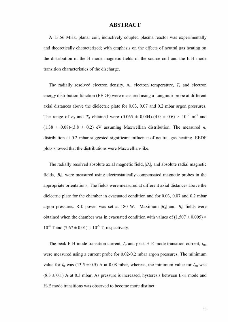
A 13.56 MHz, planar coil, inductively coupled plasma reactor was experimentally

and theoretically characterized; with emphasis on the effects of neutral gas heating on

the distribution of the H mode magnetic fields of the source coil and the E-H mode

transition characteristics of the discharge.

The radially resolved electron density, ne, electron temperature, Te and electron

energy distribution function (EEDF) were measured using a Langmuir probe at different

axial distances above the dielectric plate for 0.03, 0.07 and 0.2 mbar argon pressures.

The range of ne and Te obtained were (0.065 ± 0.004)-(4.0 ± 0.6) × 1017 m-3 and

(1.38 ± 0.08)-(3.8 ± 0.2) eV assuming Maxwellian distribution. The measured ne

distribution at 0.2 mbar suggested significant influence of neutral gas heating. EEDF

plots showed that the distributions were Maxwellian-like.

The radially resolved absolute axial magnetic field, |Bz|, and absolute radial magnetic

fields, |Br|, were measured using electrostatically compensated magnetic probes in the

appropriate orientations. The fields were measured at different axial distances above the

dielectric plate for the chamber in evacuated condition and for 0.03, 0.07 and 0.2 mbar

argon pressures. R.f. power was set at 180 W. Maximum |Bz| and |Br| fields were

obtained when the chamber was in evacuated condition with values of (1.507 ± 0.005) ×

10-4 T and (7.67 ± 0.01) × 10-5 T, respectively.

The peak E-H mode transition current, Itr and peak H-E mode transition current, Imt

were measured using a current probe for 0.02-0.2 mbar argon pressures. The minimum

value for Itr was (13.5 ± 0.5) A at 0.08 mbar, whereas, the minimum value for Imt was

(8.3 ± 0.1) A at 0.3 mbar. As pressure is increased, hysteresis between E-H mode and

H-E mode transitions was observed to become more distinct.

iv

The line averaged neutral gas temperature, Tn, was measured using a fiber probe with

the actinometry optical emission spectroscopy (AOES) technique at 0.03, 0.05, 0.07, 0.1

and 0.2 mbar argon pressure for different axial distances above the dielectric plate. R.f.

power was varied from 100 W to 200 W. The range of Tn obtained was

(350 ± 30)-(840 ± 30) K.

For theoretical characterization, two predictive models were used. The first was an

electromagnetic field model that simulates |Bz| and |Br|, using empirically fitted,

spatially resolved electron density, ne (r, z) and electron temperature, Te (r, z).

Simulations were run for spatially averaged Tn and heuristically fitted, spatially

distributed temperature, Tn (r, z). Tn (r, z) gave the closest agreement to the measured

magnetic fields.

The second model was a power deposition model that simulates Itr and Imt.

Simulations were run for Tn = 300 K and at elevated Tn. Calculations better matched the

measured values only when neutral gas heating was considered. The effect of hysteresis

in mode transition of the discharge was also demonstrated using a fitted 3D power

evolution plot.

These results indicate that neutral gas heating plays an important role in influencing

plasma parameters. Thus, knowledge of the effects of neutral gas heating is essential in

providing better understanding of the formation and maintenance of the plasma

discharge.

v

ABSTRAK

Reaktor plasma makmal yang berjanakan gegelung sesatah enam lilitan pada

frekuensi 13.56 MHz telah dicirikan secara eksperimen dan teori; dengan penekanan

diberikan kepada kesan-kesan pemanasan gas neutral terhadap taburan medan magnetik

mod H yang dijanakan oleh gegelung sesatah serta ciri-ciri peralihan mod E-H plasma.

Ketumpatan elektron, ne, suhu elektron, Te dan fungsi taburan tenaga elektron, EEDF

telah diukur mengikut jejari reaktor dengan menggunakan kuar Langmuir pada jarak

paksi berbeza di atas plet dielektrik untuk tekanan argon 0.03, 0.07 dan 0.2 mbar. Julat

ne dan Te yang diperoleh ialah (0.065 ± 0.004)-(4.0 ± 0.6) × 1017 m-3 dan

(1.38 ± 0.08)-(3.8 ± 0.2) eV dengan andaian taburan Maxwell. Ukuran taburan ne pada

tekanan 0.2 mbar telah menunjukkan pengaruh pemanasan gas neutral yang ketara.

EEDF yang diplot memberikan taburan yang menyerupai taburan Maxwell.

Medan magnet mutlak paksian, |Bz| dan medan magnet mutlak jejarian, |Br| juga telah

diukur mengikut jejari reaktor dengan mengunakan kuar magnetik lawanan elektrostatik

pada orientasi masing-masing. |Bz| dan |Br| juga telah diukur pada jarak paksi berbeza di

atas plat dielektrik untuk reaktor pada keadaan vakum dasar dan pada tekanan argon

0.03, 0.07 dan 0.2 mbar. Kuasa frekuensi radio telah ditetapkan pada 180 W. Medan |Bz|

dan |Br| maksima (masing-masing bernilai (1.507 ± 0.005) × 10-4 T dan (7.67 ± 0.01) ×

10-5 T) telah diperolehi untuk reaktor pada keadaan vakum dasar.

Arus puncak peralihan mod E ke mod H, Itr dan arus puncak peralihan mod H ke

mod E, Imt telah diukur dengan mengunakan kuar arus untuk julat tekanan argon 0.02-

0.2 mbar. Nilai minima untuk Itr ialah (13.5 ± 0.5) A pada tekanan 0.08 mbar, manakala

nilai minima untuk Imt ialah (8.3 ± 0.1) A pada tekanan 0.3 mbar. Apabila tekanan

argon meningkat, kesan histerisis di antara peralihan mod E-H dan peralihan mod H-E

bertambah ketara.

vi

Suhu purata satah gas neutral, Tn, telah diukur mengunakan kuar gentian optik

dengan teknik aktinometri spektroskopi pancaran optik (AOES) pada tekanan argon

0.03, 0.05, 0.07, 0.1 dan 0.2 mbar untuk jarak paksi berbeza di atas plet dielektrik.

Kuasa frequensi radio telah dibezakan dari 100-200 W. Julat Tn yang diperoleh ialah

(350 ± 30)-(840 ± 30) K.

Untuk pencirian teori, dua model ramalan telah digunakan. Model ramalan pertama

ialah model medan elektromagnetik yang mensimulasikan |Bz| dan |Br| dengan

mengunakan taburan ketumpatan elektron ruangan, ne (r, z) serta taburan suhu elektron

ruangan, Te (r, z) yang suaikan secara empirikal. Simulasi telah dijalankan dengan

menggunakan suhu purata Tn serta taburan suhu ruangan yang diperoleh daripada

penyesuaian heuristik, Tn (r, z). Simulasi dengan Tn (r, z) telah memberikan persetujuan

yang terbaik dengan medan magnet ukuran.

Model ramalan kedua ialah model pemendapan kuasa yang mensimulasikan Itr dan

Imt. Simulasi telah dijalankan pada suhu Tn = 300 K dan pada suhu Tn tertingkat. Nilai-

nilai simulasi lebih menyetujui nilai-nilai ukuran hanya apabila kesan pemanasan gas

neutral diambil kira. Kesan histerisis terhadap peralihan mod plasma juga telah

ditunjukkan dengan menggunakan plot evolusi kuasa 3 dimensi yang disuaikan.

Keputusan-keputusan ini menunjukkan bahawa pemanasan gas neutral memainkan

peranan penting dalam mempengaruhi parameter plasma. Oleh itu, pengetahuan tentang

kesan pemanasan gas neutral adalah penting untuk memberikan pemahaman yang lebih

baik tentang pembentukan dan pengekalan nyahcas plasma.

vii

ACKNOWLEDGEMENT

I would firstly, like to convey my heartfelt gratitude to my supervisor, Associate

Professor Dr. Chin Oi Hoong for her support and guidance towards the completion of

my Ph.D. Her presence and confidence in my abilities have given me the motivational

strength to persevere through the toughest times of my candidature.

I would also like to give my sincere appreciation to our centre’s technician Mr. Jasbir

Singh Atma Singh for his invaluable assistance, especially in purchasing and provision

of the required equipment and materials for this study.

I would next, like to extend the warmest thanks to all my peers and colleagues (in

past and in present) whom have supported me with advice and kindness. Their

friendship and camaraderie has made my journey in University Malaya a more positive

and memorable one. Special thanks to my lab mates, Choo Chee Yee, Tamilmany K.

Thandavan, Chan Li San and Siti Sarah Safaai for their help in experiments and in

situations which needed the extra pairs of hands.

I would also like to express my deepest appreciation to my parents for their

unwavering support throughout the numerous years of commitment and investment

made in pursuit of this higher degree. It is only their patience, love and encouragement

that have brought me this far in life.

I would finally, like to acknowledge the University Malaya Research Grants

(UMRG) PS329-2010A and RG135-10AFR and Short Term Research Fund (PJP)

FS280/2007C for funding of experimental and simulation work found in this thesis.

viii

LIST OF PUBLICATIONS 1. Chin, O. H., Jayapalan, K. K., & Wong, C. S. (2014, August). Effect of neutral gas

heating in argon radio frequency inductively coupled plasma. In International Journal of Modern Physics Conference Series (Vol. 32, p. 60320).

2. Jayapalan, K. K., & Chin, O. H. (2014). Effect of neutral gas heating on the wave

magnetic fields of a low pressure 13.56 MHz planar coil inductively coupled argon discharge. Physics of Plasmas, 21(4), 043510.

3. Jayapalan, K. K., & Chin, O. H. (2012). The effects of neutral gas heating on H

mode transition and maintenance currents in a 13.56 MHz planar coil inductively coupled plasma reactor. Physics of Plasmas, 19(9), 093501.

4. Jayapalan, K. K., & Chin, O. H. (2009, July). Simulation and Experimental Study

of a 13.56 MHz Planar Coil, Inductively Coupled Plasma Reactor. In Frontiers in Physics: 3rd International Meeting (Vol. 1150, No. 1, pp. 440-443).

LIST OF CONFERENCE PRESENTATIONS 1. National Physics Conference (PERFIK) 2014, Sunway Resort Hotel and Spa, Kuala

Lumpur, Malaysia: 18-19, November 2014. Contributed paper (poster presentation) titled 'Determination of Neutral Gas Temperature Using Actinometry Optical Emission Spectroscopy (AOES)'.

2. 3rd International Meeting on Frontiers of Physics (IMFP) 2009, Awana Golf and

Country Resort, Genting Highlands, Kuala Lumpur, Malaysia: 12-16th January 2009. Contributed paper (oral presentation) titled 'Simulation and experimental study of a 13.56 MHz planar coil, inductively coupled plasma reactor'.

3. 4th Mathematics and Physical Science Graduate Conference (MPSGC) 2008,

University of Malaya, Kuala Lumpur, Malaysia: 15-18 December 2008. Contributed paper (oral presentation) titled 'Hysteresis modeling for a 13.56 MHz planar coil, inductively coupled plasma system'.

4. 2nd International Conference on Science and Technology (ICSTIE) 2008-

Applications in Industry and Education, University Teknologi MARA, Pulau Pinang, Malaysia: 12-13 December 2008. Contributed paper (oral presentation) titled 'Simulation Of hysteresis between E- and H‐mode transitions for a 13.56 MHz planar coil ICP reactor'.

5. National Physics Conference (PERFIK) 2007, Heritage Bay Club, Pulau Duyong,

Kuala Terengganu, Terengganu, Malaysia: 26-28 December 2007. Contributed paper (oral presentation) titled 'Mapping of the electromagnetic field distribution in a planar coil, inductively coupled plasma reactor'.

6. 3rd Mathematics and Physical Science Graduate Conference (MPSGC) 2008,

University of Malaya, Kuala Lumpur, Malaysia: 12-14 December 2007. Contributed paper (poster presentation) titled 'Theoretical investigation of the electromagnetic field in a 13.56 MHz RF planar coil, inductively coupled plasma reactor'.

ix

TABLE OF CONTENTS

ABSTRACT iii

ABSTRAK v

ACKNOWLEDGEMENT vii

LIST OF PUBLICATIONS viii

LIST OF CONFERENCE PRESENTATIONS viii

TABLE OF CONTENTS ix

LIST OF FIGURES xiv

LIST OF TABLES xx

LIST OF SYMBOLS xxi

CHAPTER 1: INTRODUCTION 1

1.0. Introduction and Motivation of Study 1

1.1. Objectives of Study 4

1.1.1. Experiment 4

1.1.2. Simulation 5

1.2. Layout of Thesis 6

CHAPTER 2: LITERATURE REVIEW 8

2.0. History and Origins 8

2.1. E mode, H mode and Hysteresis 11

2.2. Theoretical Development and Simulation of Electrodeless Discharges and

ICPs

15

2.3. Measurement of Neutral Gas Heating and the Effects of Neutral Gas

Depletion

27

x

CHAPTER 3: EXPERIMENT 35

3.0. Experimental Setup 35

3.1. Langmuir Probe Setup 37

3.1.1. Langmuir Probe Diagnostics Setup 39

3.1.2. Langmuir Probe Theory and Analysis 40

3.2. Magnetic Probe Setup 47

3.2.1. Probe Theory and Analysis 49

3.3. Current and Voltage Probes 51

3.4. Actinometry Optical Emission Spectroscopy (AOES) Setup 52

3.4.1. AOES Theory and Analysis 53

CHAPTER 4: RESULTS, ANALYSIS AND DISCUSSION - EXPERIMENT 68

4.0. Measurement of Discharge Electrical Characteristics 68

4.0.1. Electron Density, ne and Electron Temperature, Te 68

4.0.2. Electron Energy Probability Function (EEPF) 77

4.1. Measurement of Discharge Magnetic Fields 81

4.1.1. Absolute Axial, |Bz| and Radial, |Br| Magnetic Fields 81

4.2. Measurement of Peak Coil Transition and Maintenance Currents 84

4.2.1. H Mode Peak Transition, Itr and Maintenance, Imt Currents 85

4.3. Measurement of Discharge Neutral Gas Temperature via AOES 87

4.3.1. Measured Neutral Gas Temperature, Tn 87

CHAPTER 5: SIMULATION 92

5.0. Electromagnetic Field Model 92

5.1. Analytical H mode fields 96

5.1.1. Separation of Variables Method for the H mode Fields 99

xi

5.1.2. Solving for H mode Boundary Constants 105

5.2. Numerical H mode fields

109

5.2.1. Calculation of Effective Collision Frequency, eff (r, z) 111

5.2.2. Five Point Stencil Algorithm 114

5.3. Analytical E mode fields 117

5.3.1. Separation of Variables Method for the E mode Fields 120

5.3.2. Solving for E mode Boundary Constants 124

5.4. Power Balance Model 128

5.4.1. Absorbed Electron Power, Pabs 128

5.4.2. Electron Power Loss, Ploss 131

CHAPTER 6: RESULTS, ANALYSIS AND DISCUSSION - SIMULATION 135

6.0. Predictive Simulation of the Discharge Magnetic Fields 135

6.0.1. Empirical fitting of the Spatially Resolved Electron Density, ne (r, z)

and Spatially Resolved Electron Temperature, Te (r, z)

135

6.0.2. Heuristic fitting of the Spatially Resolved Neutral Gas Temperature,

Tn (r, z)

143

6.0.3. Spatially averaged neutral gas temperatures, Tn,ave 149

6.0.4. Comparison of Measured and Simulated Magnetic Fields 149

6.1. Predictive Simulation of H mode Transition and Maintenance Currents 155

6.1.1. E-H mode Transition Dynamics and Hysteresis Effects in Discharge 155

6.1.2. Comparison of Measured H mode Transition Current, Itr and H mode

Maintenance Current, Imt with Simulation

160

CHAPTER 7: SUMMARY AND CONCLUSION 164

7.0. Overview 164

xii

7.1. Experimental Characterization

164

7.1.1. Measurement of Electron Density, ne and Electron Temperature, Te

and Electron Energy Distribution Function (EEDF)

164

7.1.2. Measurement of Absolute Axial Magnetic Field, |Bz| and Radial

Magnetic Field, |Br|

167

7.1.3. Measurement of Peak H mode Transition, Itr and H mode

Maintenance Currents, Imt

168

7.1.4. Measurement Neutral Gas Temperature, Tn 169

7.2. Theoretical Characterization 170

7.2.1. Predictive Simulation of the Discharge Magnetic Fields 171

7.2.2. Predictive Simulation of H mode Transition and Maintenance

Currents

171

7.3. Suggestions for Future Work 172

REFERENCES 175

APPENDIX A: LANGMUIR PROBE PARAMETRIC SOLVER

187

APPENDIX B: AOES Tn SOLVER 194

B.1. AOES Line Width and Line Position Convolution Solver 194

B.2. AOES Minimum 2 Neutral Gas Temperature Solver

201

APPENDIX C: ANALYTICAL H MODE FIELD MODEL

205

APPENDIX D: POWER BALANCE MODEL

212

xiii

APPENDIX E: AUXILLARY DATA AND RELATED PROGRAMS 219

E.1. Argon Collision Cross Section Spreadsheet ('ArgonCC.xls') 219

E.2. Bessel Zeros Function Code 221

E.3. Empty Excel Sheet Delete Code

223

APPENDIX F: FITTING PARAMETERS FOR SIMULATION 224

xiv

LIST OF FIGURES

Figure Caption Page

1.1

Laboratory 13.56 MHz r.f. argon ICP operating at (a) E mode and (b) H mode at 0.1 mbar.

2

1.2 The measured effects of hysteresis in the planar coil ICP reactor at 0.1 mbar argon pressure. The power required to cause a transition from E to H mode is higher (~82 W) than the power required for maintaining H mode (~ 66 W) (Lim, 2010).

2

1.3 The two types of coil configurations used in ICP design: (a) helical and (b) planar (Lieberman & Lichtenberg, 2005).

3

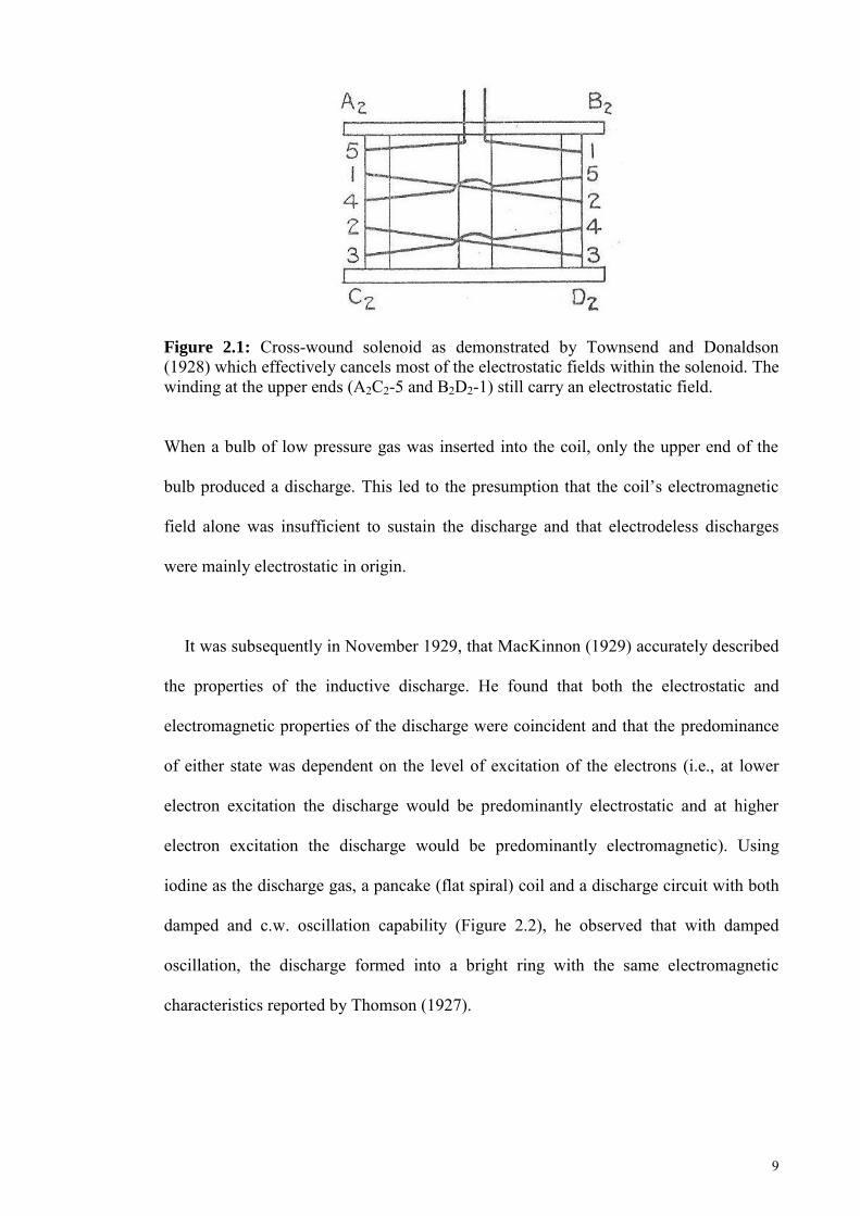
2.1 Cross-wound solenoid as demonstrated by Townsend and Donaldson (1928) which effectively cancels most of the electrostatic fields within the solenoid. The winds at the upper ends (A2C2-5 and B2D2-1) still carry an electrostatic field.

9

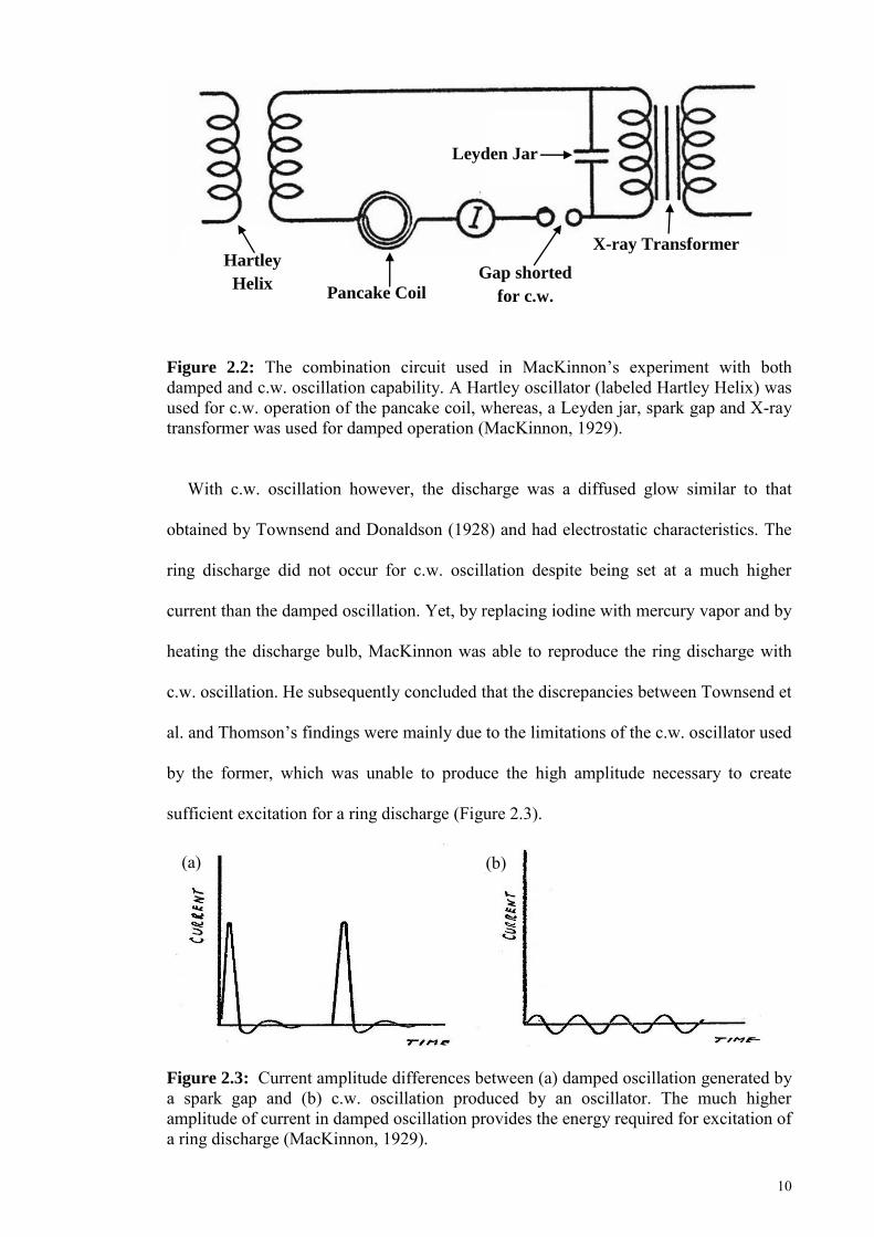
2.2 The combination circuit used in MacKinnon’s experiment with both damped and c. w. oscillation capability. A Hartley oscillator (labeled Hartley Helix) is used for c. w. operation of the pancake coil, whereas, a Leyden jar, spark gap and X-ray transformer was used for damped operation (MacKinnon, 1929).

10

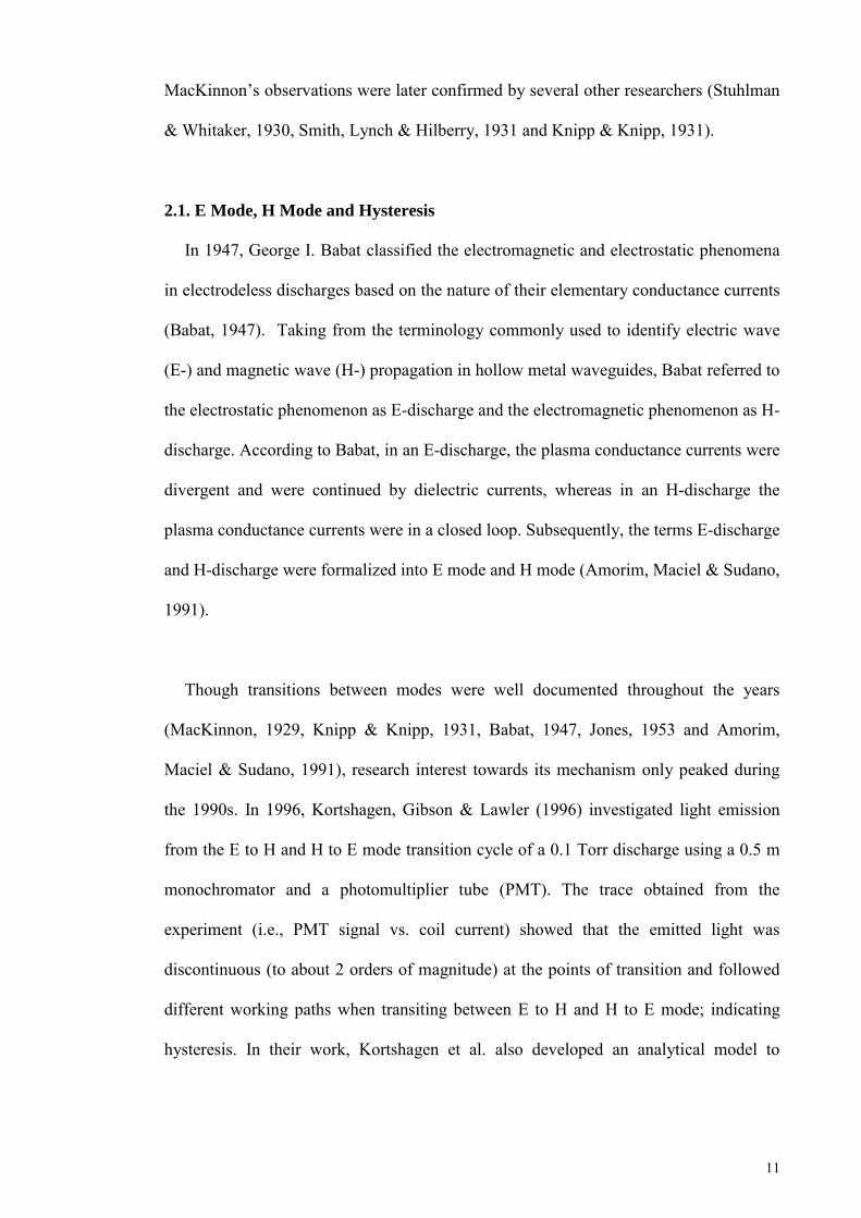
2.3 Current amplitude differences between (a) damped oscillation generated by a spark gap and (b) c. w. oscillation produced by an oscillator. The much higher amplitude of current in damped oscillation provides the energy required for excitation of a ring discharge (MacKinnon, 1929).

10

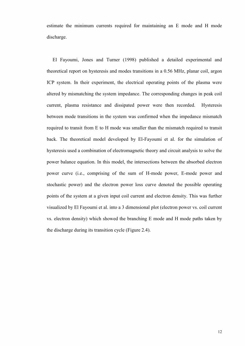
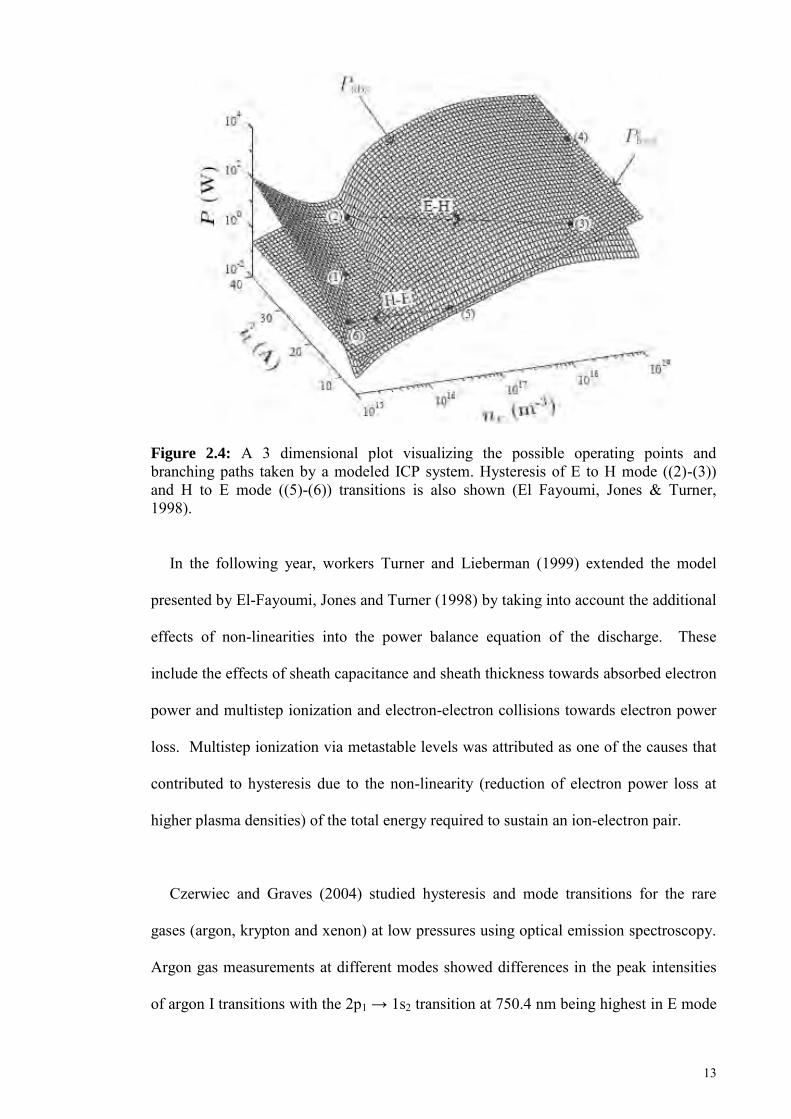
2.4 A 3 dimensional plot visualizing the possible operating points and branching paths taken by a modeled ICP system. Hysteresis of E to H mode ((2)-(3)) and H to E mode ((5)-(6)) transitions is also shown (El Fayoumi, Jones & Turner, 1998).

13

2.5 The (a) measured and (b) simulated magnetic field lines for an evacuated, planar coil, ICP source at 0.56 MHz (El Fayoumi & Jones, 1998).

20

2.6 Example of a basic Particle in Cell-Monte Carlo Collision (PIC-MCC) algorithm. Representative particles are updated for changes in their spatial properties under the influence of an electromagnetic field and by randomized collisions at discrete time steps (Birdsall, 1991).

21

2.7 Measured neutral gas density, nn (m-3) (black circles) versus radius, r (m) of an ICP reactor operating at 10 mTorr argon pressure and 2000 W power. Neutral gas depletion is seen nearing the discharge center at r = 0 m. Grey line shows the initial neutral gas density before discharge ignition (Shimada, Tynan & Cattolica, 2007).

27

xv

2.8 Graphs show (a) measured neutral gas temperature with increasing power at 0.05, 0.5 and 5 Pa and (b) measured contribution of electron pressure and gas temperature towards neutral gas depletion with increasing chamber pressure at 1000 W. Depletion of neutrals due to gas temperature becomes increasingly important as chamber pressure is increased (O’Connell et al., 2008).

31

2.9 Measured neutral gas temperature versus (a) discharge power and (b) logarithm of pressure for an argon discharge using AOES. The highest neutral gas temperature obtained was 1850 K at 600 W (Li et al., 2011).

34

3.1 Inductively Coupled Plasma (ICP) setup used for experiments.

36

3.2 Langmuir probe and mount schematics.

38

3.3 Langmuir probe diagnostics setup.

39

3.4 Measured Langmuir probe I-V signal and differential curve (d2Iprobe/dV2

probe) at 0.032 m axial height for 0.2 mbar pressure and 180 W r.f. power. I represents the ion saturation region, II represents the electron retardation region and III represents the electron saturation region. Measurement was taken at the plasma center (R = 0 m).

40

3.5 The four different current collection regimes for a Langmuir probe (Maurice, 2003).

42

3.6 Magnetic probe schematics and circuit. 48

3.7 Oscilloscope screen capture for the axial magnetic probe at 0.032 m axial distance above the dielectric plate, 0.07 mbar argon pressure and 180 W r.f. power. Measurement was taken at the plasma center (R = 0 m).

49

3.8 Axial and radial magnetic probe calibration curves.

50

3.9 Measured peak planar coil voltage, Vp,evac (V) versus peak planar coil current, Ip,evac (A) at evacuated condition.

51

3.10 AOES probe and mount schematics.

53

3.11 Measured H mode Ar/N2 emission spectra showing the nitrogen second positive system (N2C3

u-N2B3g) at 0.05 mbar pressure

(~95% Ar/~5% N2) and 200 W r.f. power. The chosen peak for simulation (0-2) is indicated.

55

3.12 Discrete synthetic spectrum for the 0-2 vibrational emission peak of the nitrogen second positive system

3 32 u 2 gN NC B at Tn = 550 K

61

3.13 Calibration curve for the HR4000 spectrometer.

61

3.14 Voigt profile fitted to the measured Hg peak at 435.8 nm. 63

xvi

3.15 The discrete synthetic spectra (a) is convolved with instrumental broadening (c) via Voigt function resulting in the convolved synthetic spectrum (b). The convolved synthetic spectrum takes the shape of the experimentally measured 0-2 vibro-rotational peak seen in Figure 3.11.

65

3.16 Demonstration of the measured spectrum intensity, x and convolved spectrum intensity, xo; interpolated to coincide with the central bin wavelength.

66

3.17 (a) χ2 plot showing minimum fitting value at 550 K (b) Experimental 0-2 vibro-rotational peak at 0.05 mbar Ar/N2 pressure and 200 W r.f. power fitted with the convolved synthetic spectrum at 550 K.

67

4.1a Maxwellian (i) electron density, ne and (ii) electron temperature, Te measured at 0.032 m distance above the dielectric plate for 0.03, 0.07 and 0.2 mbar argon pressures. R.f. power was set at 180 W.

69

4.1b EEDF (i) electron density, ne and (ii) electron temperature, Te measured at 0.032 m distance above the dielectric plate for 0.03, 0.07 and 0.2 mbar argon pressures. R.f. power was set at 180 W.

70

4.2a Maxwellian (i) electron density, ne and (ii) electron temperature, Te measured at 0.060 m distance above the dielectric plate for 0.03, 0.07 and 0.2 mbar argon pressures. R.f. power was set at 180 W.

71

4.2b EEDF (i) electron density, ne and (ii) electron temperature, Te measured at 0.060 m distance above the dielectric plate for 0.03, 0.07 and 0.2 mbar argon pressures. R.f. power was set at 180 W.

72

4.3a Maxwellian (i) electron density, ne and (ii) electron temperature, Te measured at 0.114 m distance above the dielectric plate for 0.03, 0.07 and 0.2 mbar argon pressures. R.f. power was set at 180 W.

73

4.3b EEDF (i) electron density, ne and (ii) electron temperature, Te measured at 0.114 m distance above the dielectric plate for 0.03, 0.07 and 0.2 mbar argon pressures. R.f. power was set at 180 W.

74

4.4 Electron energy probability function (EEPF) at 0.032 m distance above the dielectric plate for 0.03, 0.07 and 0.2 mbar argon pressures with corresponding parametric fit. R.f. power was at 180 W.

79

4.5 Electron energy probability function (EEPF) at 0.060 m distance above the dielectric plate for 0.03, 0.07 and 0.2 mbar argon pressures with corresponding parametric fit. R.f. power was at 180 W.

79

4.6 Electron energy probability function (EEPF) at 0.114 m distance above the dielectric plate for 0.03, 0.07 and 0.2 mbar argon pressures with corresponding parametric fit. R.f. power was at 180 W.

80

xvii

4.7 Measured absolute magnitudes of the (i) axial and (ii) radial magnetic fields at 0.032 m distance above the dielectric plate for evacuated, 0.03 mbar, 0.07 mbar and 0.2 mbar argon pressures. R.f. power was set at 180 W.

82

4.8 Measured absolute magnitudes of the (i) axial and (ii) radial magnetic fields at 0.060 m distance above the dielectric plate for evacuated, 0.03 mbar, 0.07 mbar and 0.2 mbar argon pressures. R.f. power was set at 180 W.

83

4.9 Measured H mode peak coil transition current, Itr (E-H) and H mode peak coil maintenance current, Imt (H-E) for 0.02-0.2 mbar argon pressure.

85

4.10 Measured neutral gas temperature, Tn at 0.03, 0.05, 0.07, 0.1 and 0.2 mbar Ar/N2 pressures for (i) increasing and (ii) decreasing r.f. power. Measurement was made at 0.032 m distance above the dielectric plate.

88

4.11 Measured neutral gas temperature, Tn at 0.03, 0.05, 0.07, 0.1 and 0.2 mbar Ar/N2 pressures for (i) increasing and (ii) decreasing r.f. power. Measurement was made at 0.060 m distance above the dielectric plate.

89

5.1 Numerical model diagram of the laboratory ICP reactor. 93

5.2 Analytical model diagram of the laboratory ICP reactor.

97

5.3 The five point stencil algorithm illustrated. The field values at the four adjacent (blue) grid points are used to calculate the new field value for the center (red) grid point.

114

5.4 Program flowchart for the numerical H mode fields.

116

6.1a Empirically fitted 2D Gaussian based distribution of electron density ne (r, z) used for the magnetic field simulation at 0.03 mbar argon pressure and 180 W r.f. power. (i) Fitment with measured values at 0.032 m, 0.060 m and 0.114 m distance above the dielectric plate. (ii) Modeled 2D contour plot (labels in m-3).

137

6.1b Empirically fitted 2D Gaussian based distribution of electron density ne (r, z) used for the magnetic field simulation at 0.07 mbar argon pressure and 180 W r.f. power. (i) Fitment with measured values at 0.032 m, 0.060 m and 0.114 m distance above the dielectric plate. (ii) Modeled 2D contour plot (labels in m-3).

138

6.1c Empirically fitted 2D Gaussian based distribution of electron density ne (r, z) used for the magnetic field simulation at 0.2 mbar argon pressure and 180 W r.f. power. (i) Fitment with measured values at 0.032 m, 0.060 m and 0.114 m distance above the dielectric plate. (ii) Modeled 2D contour plot (labels in m-3).

139

xviii

6.2a Empirically fitted 2D Gaussian based distribution of electron temperature Te (r, z) used for the magnetic field simulation at 0.03 mbar argon pressure and 180 W r.f. power. (i) Fitment with measured values at 0.032 m, 0.060 m and 0.114 m distance above dielectric plate. (ii) Modeled 2D contour plot (labels in eV).

140

6.2b Empirically fitted 2D Gaussian based distribution of electron temperature Te (r, z) used for the magnetic field simulation at 0.07 mbar argon pressure and 180 W r.f. power. (i) Fitment with measured values at 0.032 m, 0.060 m and 0.114 m distance above dielectric plate. (ii) Modeled 2D contour plot (labels in eV).

141

6.2c Empirically fitted 2D Gaussian based distribution of electron temperature Te (r, z) used for the magnetic field simulation at 0.2 mbar argon pressure and 180 W r.f. power. (i) Fitment with measured values at 0.032 m, 0.060 m and 0.114 m distance above dielectric plate. (ii) Modeled 2D contour plot (labels in eV).

142

6.3 Heuristically fitted 2D contour plot for spatially resolved neutral gas temperature, Tn (r, z) at (a) 0.03 mbar (b) 0.07 mbar and (c) 0.2 mbar argon pressure. Labeled temperatures are in K.

144-145

6.4 Calculated absorbed electron power, Pabs with (a) average measured electron density within the coil radius, ne,coil (m-3) and (b) calculated effective collision frequency, veff versus argon pressure.

148

6.5a Measured and simulated (i) axial magnetic fields, |Re(Bz)| and (ii) radial magnetic fields, |Re(Br)| versus radial distance, R for 0.03 mbar argon pressure at 0.032 m distance above the dielectric plate. R.f. input power was at 180 W and Ip = 14.4 A.

150

6.5b Measured and simulated (i) axial magnetic fields, |Re(Bz)| and (ii) radial magnetic fields, |Re(Br)| versus radial distance, R for 0.07 mbar argon pressure at 0.032 m distance above the dielectric plate. R.f. input power was at 180 W and Ip = 14.2 A.

151

6.5c Measured and simulated (i) axial magnetic fields, |Re(Bz)| and (ii) radial magnetic fields, |Re(Br)| versus radial distance, R for 0.2 mbar argon pressure at 0.032 m distance above the dielectric plate. R.f. input power was at 180 W and Ip = 13.4 A.

152

6.6 Simulated electron absorbed power and electron power loss versus electron density for 15 A peak r.f. coil current at 0.02 mbar argon pressure. I, II, and III represent the E mode, unstable operation, and H mode, respectively. Electron temperature, Te, neutral gas temperature, Tn, and the factor CD-M were set at 4.2 eV, 433 K and 6.6 × 104, respectively.

156

xix

6.7 A 3D plot of absorbed electron power, Pabs (magenta surface) and electron power loss, Ploss (dark blue surface) versus electron density, ne and peak coil current, Ip at 0.02 mbar argon pressure. Electron temperature, Te was set at 4.2 eV, neutral gas temperature, Tn set at 433K and CD-M = 6.6 × 104. The white arrows indicate the working path of the system, whereas the red arrows indicate mode transitions.

157

6.8 The simulated absorbed electron power (solid line) and power loss (dashed line) curves depicting (a) the current at which either E mode (13 A) or H mode operation (18 A) alone occurs.

158

6.9 The simulated absorbed electron power (solid line) and power loss (dashed line) curves depicting the threshold currents for E to H (16.41 A) and H to E (14.19 A) mode transitions.

159

6.10 Simulated (Sim.) and measured (Exp.) (a) H mode transition currents, Itr (b) H mode maintenance currents, Imt at 0.02-0.3 mbar argon pressure range.

161

xx

LIST OF TABLES Table Caption Page

2.1 Chronological summary of the theoretical development and simulation

of electrodeless discharges and ICPs. 25-26

3.1

List of parameters used to determine the probe collection regime.

44

3.2 List of rotational constants required for simulation of N2C3u-N2B3

g state transition (Huber & Herzberg, 1979, pp. 418-420).

58

3.3 Lists the line strength equations of the 3 degenerate state transitions for the rotational branches R, Q and P (Kovac, 1969).

60

6.1 Comparison of parameters of present setup with other reported works of similar ICPs.

146

6.2 Calculated values for effective collision frequency, veff and total absorbed electron power, Pabs with measured average coil electron density, ne,coil, average coil electron temperature, Te,coil and peak coil current, Ip (for 180 W input r.f. power) and set peak neutral gas temperature, Tn,peak at 0.03, 0.07 and 0.2 mbar argon pressure.

147

7.1 EEPF fitment trends at 0.03, 0.07 and 0.2 mbar argon pressure for 0.032 m, 0.060 m and 0.114 m axial distances above the dielectric plate.

167

7.2 Measured maximum and minimum Tn for increasing and decreasing r.f. power steps and different axial distances above the dielectric plate.

170

E.1 Electron energies (eV) and the corresponding argon collision cross

sections (m-2)

219-220

F.1 Empirical fitting parameters for spatially resolved electron density, ne (r, z) for different argon pressure.

224

F.2 Empirical fitting parameters for spatially resolved electron density, Te (r, z) for different argon pressure.

225

F.3 Heuristic fitting parameters for spatially resolved neutral gas temperature, Tn (r, z) for different argon pressures. Fitted Tn values were pegged at the minimum of 300 K (room temperature).

226

xxi

LIST OF SYMBOLS

Common Constants

kB = Boltzmann constant

me = Electron mass

e = Electronic charge

h = Planck’s constant

c = Speed of light

o = Free space permittivity

o = Free space permeability

MAr = Argon ion mass

nair = Refractive index of air

Common Dimensional Parameters

r, , z = Radial, azimuthal and axial cylindrical coordinates

a, d, b = Coil radius, dielectric radius and inner chamber radius

L, H, D = Effective height of chamber, full inner height of chamber and coil-chamber spacing

M, W = Height of indented cylinder and edge width of indented cylinder

R = Radial distance from chamber center (z-axis)

t = Temporal term for electromagnetic fields

Common Plasma Parameters

ne, ne,cm,

ne(r, z) = Electron density, electron density in cm, average coil electron density

and spatially resolved electron density

Te, Te,eff, Te,ave, Te(r, z)

= Electron temperature, effective electron temperature, spatially averaged electron temperature and spatially resolved electron temperature

ne,coil, Te,coil = Average coil electron density and average coil electron temperature

Tn, Tn,ave, Tn (r, z)

= Neutral gas temperature, spatially averaged neutral gas temperature, spatially resolved neutral gas temperature

xxii

mfp, en, in, ii

= Particle free mean path, electron-neutral free mean path, ion-neutral free mean path and ion-ion free mean path

Vs = Potential difference in plasma sheath

ng, ng (r, z) = Neutral gas density and spatially resolved neutral gas density

e, in = Electron-neutral total collision cross section and ion-neutral scattering cross section

Ti = Ion temperature

ln = Coulomb logarithm

P = Filling pressure or argon gas pressure

,<> = Electron energy and average electron energy

f (), EEDF = Electron energy density function

g (), EEPF = Electron energy probability function

, eff,eff (r, z)

= Collision frequency, effective collision frequency and spatially resolved effective collision frequency

p, p (r, z) = Plasma frequency and spatially resolved plasma frequency

(r, z) = Spatial conductivity parameter and spatially resolved spatial

conductivity parameter

en,ei,st

= Electron neutral collision frequency, electron ion collision frequency and stochastic collision frequency

, eff = Drive frequency and effective drive frequency

c (), c () = Collision frequency term of argon gas and collision cross section of argon gas

pi, pe = Ion pressure and electron pressure

ev = Average electron velocity

= Anomalous skin depth

uB = Bohm velocity Aeff = Effective surface area for particle loss in the reactor

hl, hr = Radial and axial plasma diffusion terms near the sheath edge

= Total energy lost per electron-ion pair created by the discharge

c, i, e = Total collisional energy loss per ion-electron pair, mean kinetic energy

lost per ion and mean kinetic energy lost per electron

xxiii

iz,ex = Argon ionization threshold energy and argon excitation threshold

energy

Kiz, Kex, Kel = Argon ionization, excitation and elastic scattering rate constants

Electrical Probe Parameters

Iion, Iion,sat = Ion current and ion saturation current

Iprobe, Vprobe,

I, V = Probe current and voltage, measured current and voltage

Vfloat, Vplasma = Floating potential and plasma potential

Ielec, Ielec,sat = Electron current and electron saturation current

Rprobe = Probe radius

lsheath = Sheath width

Ap = Probe collection area

Ip, Vp = Peak coil current and coil voltage

Ip,evac, Vp,evac = Peak coil current and coil voltage at evacuated condition

Itr, Imt = Peak E to H mode transition coil current (H mode transition current) and peak H to E mode transition coil current (H mode maintenance current)

Magnetic Probe Parameters

VCOIL1, VCOIL2, VNOISE

= Voltage signals from first (1) and second (2) winding of magnetic probe and from electrostatic noise

VMATH, VMATH, PEAK

= Differential and peak differential voltage signals from oscilloscope

VFIELD, AVE = Average magnetic field voltage

RH, NH = Helmholtz coil radius and number of coil windings

IH, PEAK, BH, PEAK

= Peak current and peak magnetic field through Helmholtz coil

mH, CH = Magnetic probe calibration constants

xxiv

Optical Emission Spectroscopy Parameters and Notations

TN2, TN2,rot = Translational temperature of nitrogen neutrals and vibro-rotational ground state temperature of the nitrogen neutrals

i = Line position of the spectral line for rotational transition branch, i = R, Q and P

i = Vibro-rotational wavenumber of the spectral line for rotational transition branch, i = R, Q and P

v, J = Vibrational and rotational quantum number

', '' = Notations for upper and lower transition states, i.e., J' is the upper state rotational quantum number

Telec, G(v), Fv(J)

= Electronic, vibrational and rotational terms for spectroscopy

v v = Electronic-vibrational constant for a single vibrational emission peak

e, exe, eye, Be, e,

e

= Vibrational and rotational constants

3x = Degenerate state for the rotational transition branches where, x = 0, 1, 2

Cspec = Parametric constant for rotational line intensity

SJ = Rotational line strength

exp, calib = Measured and standard (calibration) emission peak wavelengths

mOES COES = Optical emission spectroscopy (OES) probe/spectrometer calibration

constants

I(), I(peak) = Intensity at emission wavelength, and peak emission wavelength, peak

', peak = Emission wavelength, integration wavelength and peak emission wavelength

wl, wg, wv = Full width half maximum (FWHM) for Lorentzian, Gaussian and Voigt

functions/profiles vave = Average molecular velocity

f() = Voight function at wavelength

Iconv (),

I (') = Convoluted intensity at wavelength and intensity at the integration

wavelength,'

xxv

2 = Chi-squared statistical value

Pline = Probability (weight) of discrete lines for 2 analysis

Nbin = Total number of bins for 2 analysis

x, xo = Measured spectrum intensity and synthetic spectrum intensity at the

same wavelength

Parameters and Notations for Analytical Field Simulation

i, j = Imaginary units

, , = Time varying electric field, magnetic field and current density

E, B, J = Electric field, magnetic field and current density vectors

Er, E , Ez = Scalar radial electric field, azimuthal electric field and axial electric field components

Br, B , Bz = Scalar radial magnetic field, azimuthal magnetic field and axial magnetic field components

,K = Charge density and surface charge density terms

N = Number of turns in the coil

R(r), Z(z) = Single variable functions for separation of variables method

n = Bessel function root (subscript n denotes eigen values)

, k, q, sn, kn, qn, sn)

= Separation constants (eigen values for separation constants)

A, A1, A2, An; B, B1, B2, Bn;

C, C1, C2, Cn;

D, Dn; E, En; F, Fn; vn, un

= Boundary constants for analytical solutions of the electromagnetic fields (subscript n denotes the eigen values for the boundary constants)

Eo = Uniform radial electric field

p, r = Plasma permittivity term and dielectric constant of medium

xxvi

Parameters and Notations for Numerical Field Simulation

Δr, Δz

= Discretized radial spacing and axial spacing for numerical simulation

k = Superscript for number of iterations

n, m = Subscripts for radial and axial grid positions

Parameters for Power Balance Simulation

Pabs, Ploss = Absorbed electron power and electron power loss

Ph, Pe, Pstoc = H mode field power, E mode field power and power from stochastic heating of plasma capacitive sheath

dS = Integration term for induction coil area (Poynting vector)

*rB , *B = Complex conjugate of the radial magnetic field and complex conjugate

of the azimuthal magnetic field

S = Time averaged capacitive sheath thickness

Js = First harmonic component of current density through the sheath

Vs(r) = First harmonic component of voltage across the plasma sheath at the coil-dielectric interface

cD, cM = Druyvesteyn and Maxwellian electron-electron collision energy loss factors

CD-M = Exponential factor for the transition point between Druyvesteyn and Maxwellian EEDFs

Empirical and Heuristic Fitting Parameters

PP = EEPF fitting constants for argon pressure, P

ne,peak = Fitted peak electron density

Te,peak = Fitted peak electron temperature

Tn,peak = Fitted peak neutral gas temperature

r,ne, z,ne = Radial and axial fitting parameter for electron density

r,Te,z,Te = Radial and axial fitting parameter for electron temperature

r,Tn, z,Tn = Radial and axial fitting parameter for neutral gas temperature

1

CHAPTER 1: INTRODUCTION

1.0. Introduction and Motivation of Study

Radio frequency or r.f. inductively coupled plasmas (ICPs) have been extensively

used for the past two decades for various semiconductor processes including plasma

enhanced chemical vapor deposition (PECVD) and reactive ion etching (RIE). These

processes demand for high purity and high density plasmas which are able to give the

precise substrate modification required for fabricating present day electronic devices

(Hopwood, 1992). ICPs are induced mainly by the magnetic fields of a non-contact,

externally positioned source coil and are typically referred to as "electrodeless". The

nature of this "electrodeless" configuration allows for reduced impurities in generation

of plasma; especially in comparison to other plasmas with internal electrodes (Chen,

2008).

ICPs in practice have both capacitive and inductive means of power coupling which

together contribute towards the overall plasma. The primary mode of the plasma,

known as the H mode, is generated via predominant inductive coupling of the axial and

radial magnetic fields of the r.f. coil. The secondary mode of the plasma, known as the

E mode, is generated via capacitive axial and radial electric fields formed by the

potential difference across the coil. The E mode is usually found at lower input powers

where ionization from the potential difference of the coil is insufficient to ignite the

inductive discharge and power coupling from the electromagnetic fields of the coil is

low (Lieberman & Lichtenberg, 2005). An ICP at H mode and at E mode can be

differentiated by distinct features in electron density and luminosity (Figure 1.1). At H

mode, the plasma is highly luminous and has a high electron density (1016-1018 m3)

2

whereas, at E mode, the plasma is at low luminosity and has an electron density of about

one to two orders lower (Chabert & Braithwaite, 2011).

Figure 1.1: Laboratory 13.56 MHz r.f. argon ICP operating at (a) E mode and (b) H mode at 0.1 mbar. Transitions between E mode and H mode occur in sudden „jumps‟ of luminosity when a

threshold input power is applied. The threshold current which triggers these jumps

depends not only on external parameters (i.e., gas pressure, coil size, impedance

matching and gas type) but also on whether the input current is incremented or

decremented (Figure 1.2).

Figure 1.2: The measured effects of hysteresis in the planar coil ICP reactor at 0.1 mbar argon pressure. The power required to cause a transition from E to H mode is higher (~82 W) than the power required for maintaining H mode (~ 66 W) (Lim, 2010).

(a) (b)

3

This hysteresis phenomenon has become a point of interest for many researchers in this

field of study and is well documented (Cunge, et al., 1999, Daltrini et al., 2008, El-

Fayoumi, Jones & Turner, 1998, and Xu, et al., 2000).

The magnetic fields required for formation of an ICP can be generated from either

one of two types of source coil configurations, i.e., the helical coil configuration or the

planar coil configuration (Figure 1.3).

Figure 1.3: The two types of coil configurations used in ICP design: (a) helical and (b) planar (Lieberman & Lichtenberg, 2005).

For industrial ICPs, the planar coil configuration is preferred due to the distribution of

the induced fields which results in higher uniformity in power deposition and plasma

density (Steward, et al., 1995 and Xu, et al., 2001). In material processing applications

such as PECVD and RIE, a silicon substrate is typically placed in the vicinity of the

plasma to be treated by ion bombardment. With a higher uniformity in plasma density,

better process control is achieved in terms of reproducibility and evenness of substrate

treatment (Ogle, 1990). The optimization and simulation of the source magnetic fields

for control of plasma uniformity has been a frequent subject of applied ICP research

(Cuomo et al., 1994, Hopwood et al., 1993, Patrick et al., 1995, Paranjpe, 1994, and El-

Fayoumi & Jones, 1998).

Helical Coil

Planar Coil (a) (b)

4

In recent years, spectroscopic measurement techniques have revealed that ICP

neutral gas temperatures are much higher than the previously stipulated near-room

temperatures commonly associated with low temperature discharges. Measurements

made by Li et al. (2011) for argon ICPs have shown neutral gas temperatures of up to

1750 K for the r.f. input power 200 W. In simulation, intrinsic ICP parameters such as

electron density and electron temperature have been reported to be influenced by

elevated neutral gas temperatures; with comparison of measured results and simulation

giving better agreement (Hash et al., 2001 and Ostrikov, et al., 2002). Temperature

effects on extrinsic ICP parameters, such as magnetic field distribution and discharge

mode transitions, however, have yet to be explicitly characterized. Thus, in this work,

the effects of neutral gas temperature on these parameters will be experimentally and

theoretically studied.

1.1. Objectives of Study

This study aims to experimentally and theoretically characterize the effects of neutral

gas heating on key ICP parameters; with focus on predictive simulation of the discharge

magnetic fields and E-H mode transition currents at elevated temperature. The study is

divided into two parts:

1.1.1. Experiment

For experiment, the following plasma parameters will be measured with several

diagnostic probes and techniques:

(a) Electron density, ne and electron temperature, Te

A laboratory Langmuir probe will be used to measure the radially resolved electron

density, ne and electron temperature, Te at 0.032, 0.060 and 0.114 m axial distances

5

above the dielectric plate for 0.03, 0.07 and 0.2 mbar argon pressures. R.f. power is set

at 180 W. The electron energy density distribution (EEDF) is also measured at the

chamber center for all cases.

(b) Absolute axial magnetic field, |Bz| and radial magnetic field, |Br|

Two electrostatically compensated magnetic probes will be used to measure the

absolute axial magnetic field, |Bz| and radial magnetic field |Br| magnitudes at 0.032 and

0.060 m axial distances above the dielectric plate for 0.03, 0.07 and 0.2 mbar argon

pressures. R.f. power is set at 180 W.

(c) H mode transition current, Itr and H mode maintenance current, Imt

A current probe will be used to measure the H mode transition current, Itr and H

mode maintenance current, Imt at the argon pressure range of 0.02-0.3 mbar.

(d) Neutral gas temperature, Tn

An optical fiber probe will be used to measure the neutral gas temperature, Tn via

actinometry optical emission spectroscopy (AOES) technique. Measurements will be

made at 0.03, 0.05, 0.07, 0.1 and 0.2 mbar Ar/N2 pressures for 0.032 m and 0.060 m

axial distances above the dielectric plate and for increasing and decreasing steps of r.f.

power, i.e., 100-200 W and 200-100 W.

1.1.2. Simulation

For simulation, two models will be developed based on existing derivations, i.e., the

electromagnetic model (El-Fayoumi & Jones, 1998) and the power balance model (El-

Fayoumi, Jones & Turner, 1998):

6

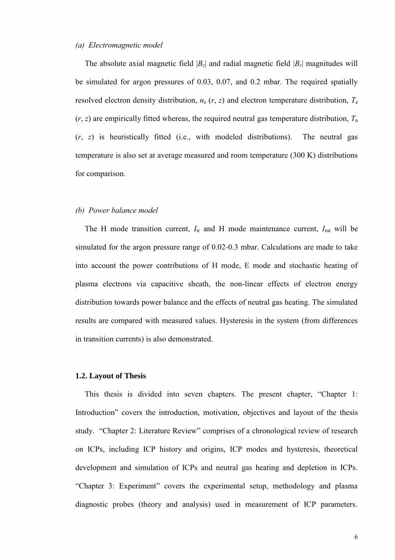
(a) Electromagnetic model

The absolute axial magnetic field |Bz| and radial magnetic field |Br| magnitudes will

be simulated for argon pressures of 0.03, 0.07, and 0.2 mbar. The required spatially

resolved electron density distribution, ne (r, z) and electron temperature distribution, Te

(r, z) are empirically fitted whereas, the required neutral gas temperature distribution, Tn

(r, z) is heuristically fitted (i.e., with modeled distributions). The neutral gas

temperature is also set at average measured and room temperature (300 K) distributions

for comparison.

(b) Power balance model

The H mode transition current, Itr and H mode maintenance current, Imt will be

simulated for the argon pressure range of 0.02-0.3 mbar. Calculations are made to take

into account the power contributions of H mode, E mode and stochastic heating of

plasma electrons via capacitive sheath, the non-linear effects of electron energy

distribution towards power balance and the effects of neutral gas heating. The simulated

results are compared with measured values. Hysteresis in the system (from differences

in transition currents) is also demonstrated.

1.2. Layout of Thesis

This thesis is divided into seven chapters. The present chapter, “Chapter 1:

Introduction” covers the introduction, motivation, objectives and layout of the thesis

study. “Chapter 2: Literature Review” comprises of a chronological review of research

on ICPs, including ICP history and origins, ICP modes and hysteresis, theoretical

development and simulation of ICPs and neutral gas heating and depletion in ICPs.

“Chapter 3: Experiment” covers the experimental setup, methodology and plasma

diagnostic probes (theory and analysis) used in measurement of ICP parameters.

7

“Chapter 4: Results and Discussion - Experiment” discusses the immediate results and

findings obtained from measurement. Derivations of equations for electromagnetic and

power balance models along with methodology for numerical simulation are covered in

“Chapter 5: Simulation”. “Chapter 6: Results and Discussion - Simulation” discusses

the key results and findings of predictive simulation using measured and empirically

fitted parameters from Chapter 4 and the derived models from Chapter 5. The thesis is

concluded with “Chapter 7: Summary and Conclusion” which gives the summaries and

conclusions drawn from the results obtained in Chapters 4 and 6.

8

CHAPTER 2: LITERATURE REVIEW

2.0. History and Origins

The advent of research in inductively coupled discharges began with the discovery of

the ‘electrodeless ring discharge’ by Johann Wilhelm Hittorf (Hittorf, 1884). In

Hittorf’s experiment, a Leyden jar and spark gap was used to send sparks (or damped

oscillating pulses) at high frequency through a wire which was coiled helically around a

vacuum tube; resulting in a bright ring shaped discharge. Hittorf attributed the

formation of the discharge to the excitation of electrons by the electromagnetic fields of

the coil. More detailed experimentation and explanation towards this phenomenon was

later done by Sir J. J. Thomson (Thomson, 1927). Sir Thomson’s work included the

effects of light and gas impurities towards discharge maintenance and the development

of a theory which describes the discharge’s electromagnetic characteristics. His

derivations also highlighted the dependence of the discharge ignition on input spark

frequency and tube gas pressure. His theoretical work, however, was disputed the

following year by Townsend and Donaldson (1928). They argued that the calculated

electrostatic field intensity between the ends of a typical solenoid was more than 30

times larger than its electromagnetic field intensity and thus, the cause of the discharge

was predominantly electrostatic. This notion was also demonstrated experimentally by

using a continuous wave (c.w.) oscillator (i.e., replacing the previous Leyden jar and

spark gap) which was connected to a cross-wound solenoid. The solenoid was wound in

a manner that cancels out much of the electrostatic field (Figure 2.1); leaving only

electromagnetic fields within the coil. The upper end of the coil which was unwound

however, still had electrostatic fields.

9

Figure 2.1: Cross-wound solenoid as demonstrated by Townsend and Donaldson (1928) which effectively cancels most of the electrostatic fields within the solenoid. The winding at the upper ends (A2C2-5 and B2D2-1) still carry an electrostatic field. When a bulb of low pressure gas was inserted into the coil, only the upper end of the

bulb produced a discharge. This led to the presumption that the coil’s electromagnetic

field alone was insufficient to sustain the discharge and that electrodeless discharges

were mainly electrostatic in origin.

It was subsequently in November 1929, that MacKinnon (1929) accurately described

the properties of the inductive discharge. He found that both the electrostatic and

electromagnetic properties of the discharge were coincident and that the predominance

of either state was dependent on the level of excitation of the electrons (i.e., at lower

electron excitation the discharge would be predominantly electrostatic and at higher

electron excitation the discharge would be predominantly electromagnetic). Using

iodine as the discharge gas, a pancake (flat spiral) coil and a discharge circuit with both

damped and c.w. oscillation capability (Figure 2.2), he observed that with damped

oscillation, the discharge formed into a bright ring with the same electromagnetic

characteristics reported by Thomson (1927).

10

Figure 2.2: The combination circuit used in MacKinnon’s experiment with both damped and c.w. oscillation capability. A Hartley oscillator (labeled Hartley Helix) was used for c.w. operation of the pancake coil, whereas, a Leyden jar, spark gap and X-ray transformer was used for damped operation (MacKinnon, 1929).

With c.w. oscillation however, the discharge was a diffused glow similar to that

obtained by Townsend and Donaldson (1928) and had electrostatic characteristics. The

ring discharge did not occur for c.w. oscillation despite being set at a much higher

current than the damped oscillation. Yet, by replacing iodine with mercury vapor and by

heating the discharge bulb, MacKinnon was able to reproduce the ring discharge with

c.w. oscillation. He subsequently concluded that the discrepancies between Townsend et

al. and Thomson’s findings were mainly due to the limitations of the c.w. oscillator used

by the former, which was unable to produce the high amplitude necessary to create

sufficient excitation for a ring discharge (Figure 2.3).

Figure 2.3: Current amplitude differences between (a) damped oscillation generated by a spark gap and (b) c.w. oscillation produced by an oscillator. The much higher amplitude of current in damped oscillation provides the energy required for excitation of a ring discharge (MacKinnon, 1929).

Pancake Coil

(a) (b)

Hartley

Helix

Leyden Jar

Gap shorted

for c.w.

X-ray Transformer

11

MacKinnon’s observations were later confirmed by several other researchers (Stuhlman

& Whitaker, 1930, Smith, Lynch & Hilberry, 1931 and Knipp & Knipp, 1931).

2.1. E Mode, H Mode and Hysteresis

In 1947, George I. Babat classified the electromagnetic and electrostatic phenomena

in electrodeless discharges based on the nature of their elementary conductance currents

(Babat, 1947). Taking from the terminology commonly used to identify electric wave

(E-) and magnetic wave (H-) propagation in hollow metal waveguides, Babat referred to

the electrostatic phenomenon as E-discharge and the electromagnetic phenomenon as H-

discharge. According to Babat, in an E-discharge, the plasma conductance currents were

divergent and were continued by dielectric currents, whereas in an H-discharge the

plasma conductance currents were in a closed loop. Subsequently, the terms E-discharge

and H-discharge were formalized into E mode and H mode (Amorim, Maciel & Sudano,

1991).

Though transitions between modes were well documented throughout the years

(MacKinnon, 1929, Knipp & Knipp, 1931, Babat, 1947, Jones, 1953 and Amorim,

Maciel & Sudano, 1991), research interest towards its mechanism only peaked during

the 1990s. In 1996, Kortshagen, Gibson & Lawler (1996) investigated light emission

from the E to H and H to E mode transition cycle of a 0.1 Torr discharge using a 0.5 m

monochromator and a photomultiplier tube (PMT). The trace obtained from the

experiment (i.e., PMT signal vs. coil current) showed that the emitted light was

discontinuous (to about 2 orders of magnitude) at the points of transition and followed

different working paths when transiting between E to H and H to E mode; indicating

hysteresis. In their work, Kortshagen et al. also developed an analytical model to

12

estimate the minimum currents required for maintaining an E mode and H mode

discharge.

El Fayoumi, Jones and Turner (1998) published a detailed experimental and

theoretical report on hysteresis and modes transitions in a 0.56 MHz, planar coil, argon

ICP system. In their experiment, the electrical operating points of the plasma were

altered by mismatching the system impedance. The corresponding changes in peak coil

current, plasma resistance and dissipated power were then recorded. Hysteresis

between mode transitions in the system was confirmed when the impedance mismatch

required to transit from E to H mode was smaller than the mismatch required to transit

back. The theoretical model developed by El-Fayoumi et al. for the simulation of

hysteresis used a combination of electromagnetic theory and circuit analysis to solve the

power balance equation. In this model, the intersections between the absorbed electron

power curve (i.e., comprising of the sum of H-mode power, E-mode power and

stochastic power) and the electron power loss curve denoted the possible operating

points of the system at a given input coil current and electron density. This was further

visualized by El Fayoumi et al. into a 3 dimensional plot (electron power vs. coil current

vs. electron density) which showed the branching E mode and H mode paths taken by

the discharge during its transition cycle (Figure 2.4).

13

Figure 2.4: A 3 dimensional plot visualizing the possible operating points and branching paths taken by a modeled ICP system. Hysteresis of E to H mode ((2)-(3)) and H to E mode ((5)-(6)) transitions is also shown (El Fayoumi, Jones & Turner, 1998).

In the following year, workers Turner and Lieberman (1999) extended the model

presented by El-Fayoumi, Jones and Turner (1998) by taking into account the additional

effects of non-linearities into the power balance equation of the discharge. These

include the effects of sheath capacitance and sheath thickness towards absorbed electron

power and multistep ionization and electron-electron collisions towards electron power

loss. Multistep ionization via metastable levels was attributed as one of the causes that

contributed to hysteresis due to the non-linearity (reduction of electron power loss at

higher plasma densities) of the total energy required to sustain an ion-electron pair.

Czerwiec and Graves (2004) studied hysteresis and mode transitions for the rare

gases (argon, krypton and xenon) at low pressures using optical emission spectroscopy.

Argon gas measurements at different modes showed differences in the peak intensities

of argon I transitions with the 2p1 → 1s2 transition at 750.4 nm being highest in E mode

14

and the 2p3 → 1s5 transition at 763.51 nm and the 2p9 → 1s5 transition at 811.53 nm

being highest in H-mode. The shift in peak intensities of the argon emission lines were

linked to the added role of metastable excitation states. The hysteresis loop (E to H

mode and H to E mode) of argon and krypton were also demonstrated.

Also in 2004, the temporal dynamics of E to H mode transition for argon plasma at

atmospheric pressure were examined by researchers Razzak et al. (2004) using a 4500

f/s high speed camera (FASTCAM-ultima SE) and CCD camera. From experimental

investigation, they found that on E to H mode transition, the E mode plasma develops

multiple streamer-like discharges of axial direction which were subsequently,

transformed into a bright ring which forms the H mode plasma. Transition dynamics

was also seen in the behavior of the plasma loading impedance, whereby an almost

linear increase in loading impedance was observed during E to H mode transition. In

this study, Razzak et al. also developed a theoretical model to estimate transition time

(400-900 ms) which showed good agreement with the experimentally measured range

(500-1000 ms).

Daltrini et al. (2008) discovered that hysteresis in inductively coupled plasmas was

mostly due to power losses in the system’s impedance matching network. It was found

that when plasma parameters (i.e., electron density, electron temperature, argon

metastable density and ion density) were plotted against plasma power (corrected for

coil and hardware losses) instead of input r.f. power, no hysteresis was observed. It was

also seen that when plotting against corrected plasma power, an inaccessible region was

formed between modes at which no stable discharge was produced.

15

The influence of impedance matching on hysteresis and mode transitions was also

shown by workers Gao et al. (2010) in their report which demonstrated the relationship

between matching network capacitance and plasma parameters. In their experiment at

30 mTorr and 100 mTorr argon pressure, the capacitance of a -type matching network

capacitor was varied between 114-127 pF and the corresponding changes of input

current, input voltage, forward power, phase angle and plasma density were recorded. It

was found that the increase in matching capacitance expanded the hysteresis loop of

circuit parameters and plasma density (versus applied power). Also, at higher matching

capacitances (120.0 pF, 121.2 pF and 123.3 pF), the hysteresis loop for input current

was found to be inverse, i.e., E to H mode transition caused a jump from lower to higher

input current instead of the expected higher to lower jump.

Lee, Kim and Chung (2013) demonstrated the absence of hysteresis between mode

transitions when using an automated matching network (which removes system

impedance matching discrepancies) at 13.56 MHz r.f. frequency and 100 mTorr argon

pressure. However, when the same experiment was run at 350 mTorr argon pressure,

hysteresis was still observed. Lee et al. attributed this to the effects of non-linear power

balance which occurs more distinctly at higher pressures. It was thus, concluded that

both impedance matching and non-linear power balance play a part in contributing to

the hysteresis phenomenon.

2.2. Theoretical Development and Simulation of Electrodeless Discharges and ICPs

The first theoretical treatment for the electromagnetic fields of an electrodeless

discharge was given by Thomson (1927). Sir Thomson correlated the peak cyclotron

velocity of a single plasma electron with the ionization potential of the discharge,

stating that the discharge will only be initiated if the electron reaches the minimum

16

kinetic velocity given by the ionization potential. He further concluded that in order to

obtain this velocity, the initiating electron must not encounter collisions from other

particles; thus, deriving the threshold pressure required to initiate the discharge from the

free mean path of the electron. Thomson (1930), derived from the input oscillating

electric fields, the conditions of electron ionization energy, discharge tube length,

pressure and ion recombination rate required to maintain an electrodeless discharge.

These maintenance conditions were shown to hold good approximation with available

experimental data (Kirchner, 1925).

Townsend (1932) developed a parallel plate model describing the electrostatically

driven electrodeless discharge. The discharge was assumed to occur in a quartz chamber

midway between two parallel plate electrodes with a high frequency oscillating electric

field. Townsend derived the analytical approximations for electron density and electron

excitation energy in terms of the mean electrostatic force between particles and electron

diffusion and ionization coefficients. The expansion to Thomson’s (1927)

electromagnetic theory for electrodeless discharges was later done by Kunz (1932).

Kunz derived the electromagnetically induced ring current of the discharge and also

circuit parameters such as self inductance, mutual inductance, oscillation frequency

difference (with and without plasma) and discharge conductivity. He also included the

derivations of discharge conductivity and self inductance for the electrostatic case.

Kunz’s circuit theory of the electrodeless discharge can be said to be the precursor of

modern day circuit theory for ICPs.

Eckert (1962) published a paper detailing a plasma diffusion theory for electrodeless

discharges based on Schottky’s (1924) electron balance solution for the positive plasma

column. The experimental parameters for hydrogen were used to illustrate the theory.

17

From the model, Eckert deduced that the maximum obtainable electron density for an

electrodeless discharge was strongly dependent on the product of discharge frequency

and magnetic field, moderately dependent on gas pressure and independent of chamber

radius. Henriksen, Keefer and Clarkson (1971) derived a closed form solution of the

electromagnetic fields for a low pressure electrodeless discharge using non-uniform

complex plasma conductivity with a parabolic distribution. The magnitude of field

variations within the discharge were found to be qualitatively similar to previous studies

which generally assumed uniform and weakly reactive (real) plasma conductivity

(Thomson, 1927 and Eckert, 1962). Two years later, Keefer, Sprouse and Loper (1973)

solved the 1D cylindrical energy balance equation for a confined, inductive

electrodeless arc with the consideration of convective energy transport due to radial

inflow of gas. Using experimental values of electrical and thermal conductivity and

specific radiation for argon at atmospheric pressure, the arc temperature profile

calculated by Keefer’s model (i.e., with convection) showed better agreement with

experimental results compared to a reference model without convection.

Boulos (1976) presented a model which calculates the 2D flow and temperature

fields of an atmospheric, argon inductive plasma torch at 3 MHz r.f. frequency and 3.77

kW power. The simulated coil was helical and of radius, 2.4 cm. The corresponding

momentum, continuity and energy equations were solved simultaneously using 1D

magnetic and electric field equations. Results demonstrated the existence of a magnetic

pumping effect (via recirculation eddy currents) which was responsible for radial inflow

at the center of the coil. Back flow at the upstream end of the coil was of the order of 20

ms-1 and was responsible for particle repulsion in the area. Significant reduction of heat

flux to the plasma tube was also seen when gas flow rate was increased. The model was

further expanded by Mostaghimi and Boulos (1989) to include 2D electromagnetic

18

fields which enabled the prediction of coil geometry effects on the flow and temperature

fields of the discharge.

Vahedi et al. (1995) derived a simple analytical model to describe power deposition

in a cylindrical inductively coupled plasma source with a planar coil. The model was

valid of all collisionality regimes of the plasma, i.e., with both ohmic (collisional)

heating and stochastic (collisionless) heating components considered. An effective

electron collision frequency with contributions from both components was devised for

this purpose. From the model, it was concluded that stochastic heating had a dominant

influence in power deposition for ICPs at low pressure.

In the same year, Li, Wu and Chen (1995) developed a time averaged two-

dimensional fluid model for a planar coil inductive plasma source which included an

electromagnetic module with self-consistent power deposition to calculate transport

parameters. Some of the assumptions made for the model were negligible gas flow,

Maxwellian electron energy density function (EEDF), equal ion and neutral temperature

and spatially uniform neutral gas temperature and distribution. The planar spiral coil

was simulated as three co-axial flat circular coils. Li et al. simulated the plasma density,

electron temperature, azimuthal electric field intensity, plasma potential and ionization

rate spatial profiles for the case of 500 W r.f power and 10 mTorr neutral gas pressure.

The effects of gas pressure and plasma power on electron temperature and electron

density were also demonstrated i.e., with the electron temperature increasing slightly

with plasma power and decreasing slightly with pressure and the electron density

increasing linearly with both parameters. These simulated trends were in accordance to

experimentally measured results by Hopwood et al. (1993).

19

Gudmundsson and Lieberman (1998) calculated the effective electron collision

frequency, electron density and electron temperature of planar coil argon plasma using

an axis symmetric, global volume-averaged discharge model. In a global model,

spatially varying experimental parameters, such as electron density and electron

temperature were assumed to be of a predefined value or distribution (i.e., for

simplicity). In this model, the electron density was assumed to be the average value

across the chamber radius, with exception of the boundaries whereby the density values

fall sharply. Three component collision frequencies, i.e., electron-neutral, electron-ion

and stochastic collision frequency were used to calculate the effective electron collision

frequency. Using the electron power balance equation and calculated plasma

parameters, Gudmundsson et al. determined the mutual inductance, self inductance,

plasma resistance and inertia inductance of the discharge as a function of skin depth and

absorbed plasma power. Calculated values of induced plasma current (derived from

plasma resistance) provided a reasonable estimate to experimental values measured by

El-Fayoumi and Jones (1997).

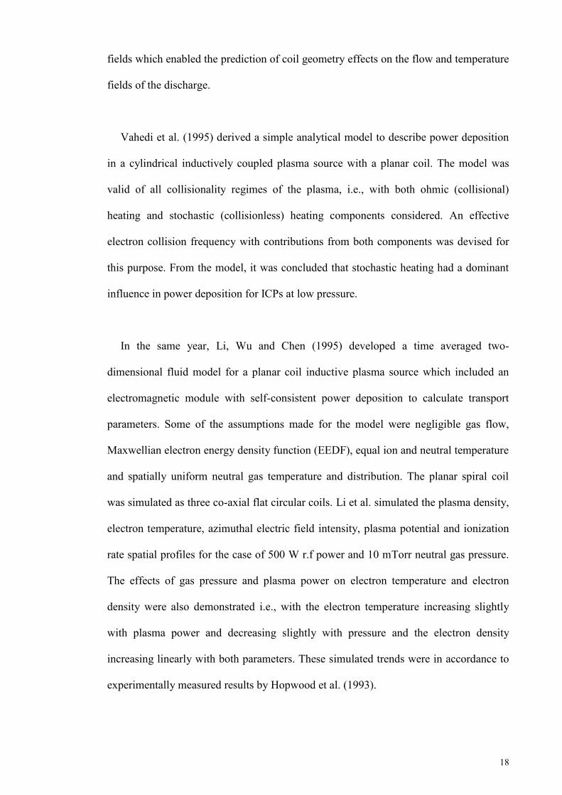
El-Fayoumi and Jones (1998), also presented a comprehensive theoretical treatment

of the spatial distribution of the H mode fields within a 0.56 MHz, planar coil, ICP

source. The azimuthal electric, radial magnetic and axial magnetic fields were solved

analytically for the cases of evacuated and plasma filled chamber with constant electron

density. The case of a spatially varying electron density was also solved using the

method of finite difference. Temporo-spatial magnetic field lines were visualized and

compared for both measured (Figure 2.5 (a)) and simulated (Figure 2.5 (b)) fields. El-

Fayoumi et al. also compared the measured and simulated phase variations at different

radial distances from the chamber center. From comparisons, it was concluded that

20

within a factor of two, meaningful information of plasma properties can be deduced by

the analysis of magnetic field data.

Figure 2.5: The (a) measured and (b) simulated magnetic field lines for an evacuated, planar coil, ICP source at 0.56 MHz (El Fayoumi & Jones, 1998).

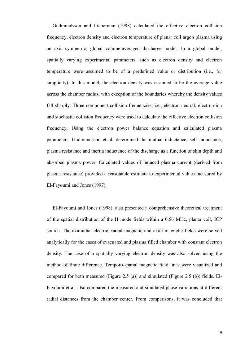
Nanbu (2000) compiled a review article on kinetic particle simulation of low

pressure, high density plasma sources which included ICPs. In the simulation, Nanbu

solved the kinetic Boltzmann transport equation using the method of particle-in-cell

(PIC) (Birdsall, 1991), i.e., a method in which 1000s of representative particles were

generated and moved within predetermined spatial grids at discrete time steps.

Displacement and velocity of the particles (by influence of the electromagnetic fields of

the source) were determined using the Lorentz force equation. Collisional processes

which occur during particle movement were treated using Monte Carlo (Birdsall, 1991)

and direct simulation Monte Carlo schemes (Serikov, Kawamoto & Nanbu 1999); both

of which were probabilistic methods of determining the type of collision (Figure 2.6).

(a) (b)

21

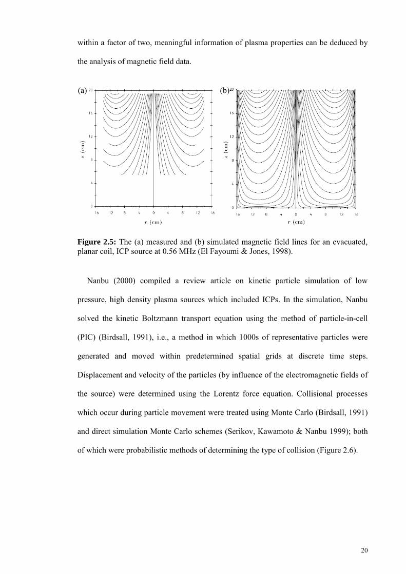
Figure 2.6: Example of a basic Particle in Cell-Monte Carlo Collision (PIC-MCC) algorithm. Representative particles are updated for changes in their spatial properties under the influence of an electromagnetic field and by randomized collisions at discrete time steps (Birdsall, 1991).

Collisional processes considered in Nanbu’s simulation were extensive, included

were electron-molecule and ion-molecule collisions (which include elastic collisions,

excitation and ionization), molecule-molecule hard sphere collisions and Coulomb

collisions (electron-electron, ion-ion and ion-electron charge based influence on particle

movement). Trajectory and velocity of particles were adjusted according to the

collisional influences of each time step. In these simulations, were illustrated the

influence of the different types of collisions on the statistical distribution of electron

energy of argon plasma via electron energy distribution function (EEDF). The number

density distributions of CF3+, CF3

-, F- and electrons of a simulated CF3 discharge were

also shown.

Panagopoulos et al. (2002) developed a 3D cylindrical, finite element fluid model

(MPRES-3D) to study azimuthal asymmetries in inductively coupled plasmas and its

effects on ion etch uniformity in etching applications. The model was made up of

several iteration modules that repeatedly compute the electromagnetic, electron energy,

22

particle transport, particle flux and sheath equations in a cyclical fashion till a

convergence was reached. The power deposition, electrostatic potential, electron

temperature, particle densities, etch rate and etch uniformity was calculable from the

converged solution. Silicon wafer etching with chlorine in a planar coil reactor was

simulated for four different cases, i.e., azimuthally uniform power deposition without a

focus ring, azimuthally uniform power deposition with a focus ring, non-uniform power

deposition without a focus ring and non-uniform power deposition with a focus ring.

The power deposition profiles, Cl+ densities and Cl densities were compared at 14 cm

from the wafer plane and at the wafer plane. The etch rate distributions were also

compared. It was found that when the etching was ion driven, etch uniformity was

strongly dependent on the power deposition profile. For the cases with uniform power

deposition, however, asymmetric pumping (of discharge gas) became a more prominent

factor for etch uniformity. The cases simulated with a focus ring had significantly

reduced azimuthal non-uniformities compared to the cases without.

Nam and Economou (2004) developed a two dimensional self consistent fluid model

for the miniaturized inductively coupled plasma (mICP) presented by Hopwood,

Minayeva and Yin (2000). The chamber was 5 mm in radius and 6 mm in length with a

planar coil of diameter of 5 mm. The equations of plasma power deposition, electron

temperature and particle species were solved for 370-770 mTorr argon pressure and 0-

1.3 W r.f. power at 450 MHz. The plasma electrons in the model were assumed to be

Maxwellian and the plasma sheath was not taken into consideration. The simulated

electron temperature distribution was found to peak at the power deposition region near

the coil. Warm electrons were also observed to persist outside the deposition region due

to the high thermal conductivity of the plasma area. Nam et al. also noted that Langmuir

probe measurements would be challenging due to the strong ion density gradients seen

23

in the simulation. Comparisons between experimental and theoretical results for ion and

electron density and temperature were of reasonable agreement.

Takao et al. (2010) developed a two-dimensional axis-symmetric PIC-MCC model to

simulate the same mICP source developed by Hopwood, Minayeva and Yin (2000).

Two types of power deposition schemes (i.e., collisional and kinetic) were used to

simulate coupling between the r.f. fields and the plasma. The collisional scheme used

the cold electron approximation and the electron velocity distribution to solve plasma

power deposition whereas the kinetic scheme used the current density calculated

directly from particle trajectories to solve plasma power deposition. Calculations were

performed at 370-770 mTorr pressure at the rf frequency of 450 MHz for powers below

3.5 W. Results were compared to the experimental data measured by Hopwood et al.

and the fluid model developed by Nam and Economou (2004). The spatial plasma

density distribution of the simulation was found to be close to the Nam and Economou

fluid model in which steep gradient densities were obtained. Takao et al. also found that

the plasma sheath was non-negligible in simulation and sheath thickness was almost

10% of the simulated reactor length. The electron energy density distribution of the

plasma was non-Maxwellian throughout the entire plasma region with depletion at

higher electron energies due to inelastic collisions. Non-consideration of the sheath and

assumption of Maxwellian electrons in the Nam and Economou fluid model showed

electron temperature distribution that was different from the Takao et al.’s PIC-MCC

model. Pressure dependence of the plasma density also showed different tendency

between the collisional and kinetic schemes in the PIC-MCC model with the collisional

scheme showing decrease of plasma density and the kinetic scheme showing increase of

plasma density with increasing pressure. The collisional scheme did not reflect the trend

shown in experiment and this was attributed by Takao et al. to be due to the inadequacy

24

of the collisional model which did not consider the effects of non-collisional heating

processes.

The chronological development of ICP simulation and theory (as detailed in this

section) is summarized in Table 2.1.

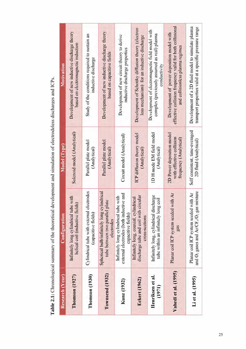
25

Tab

le 2

.1: C

hron

olog

ical

sum

mar

y of

the

theo

retic

al d

evel

opm

ent a

nd si

mul

atio

n of

ele

ctro

dele

ss d

isch

arge

s and

ICPs

.

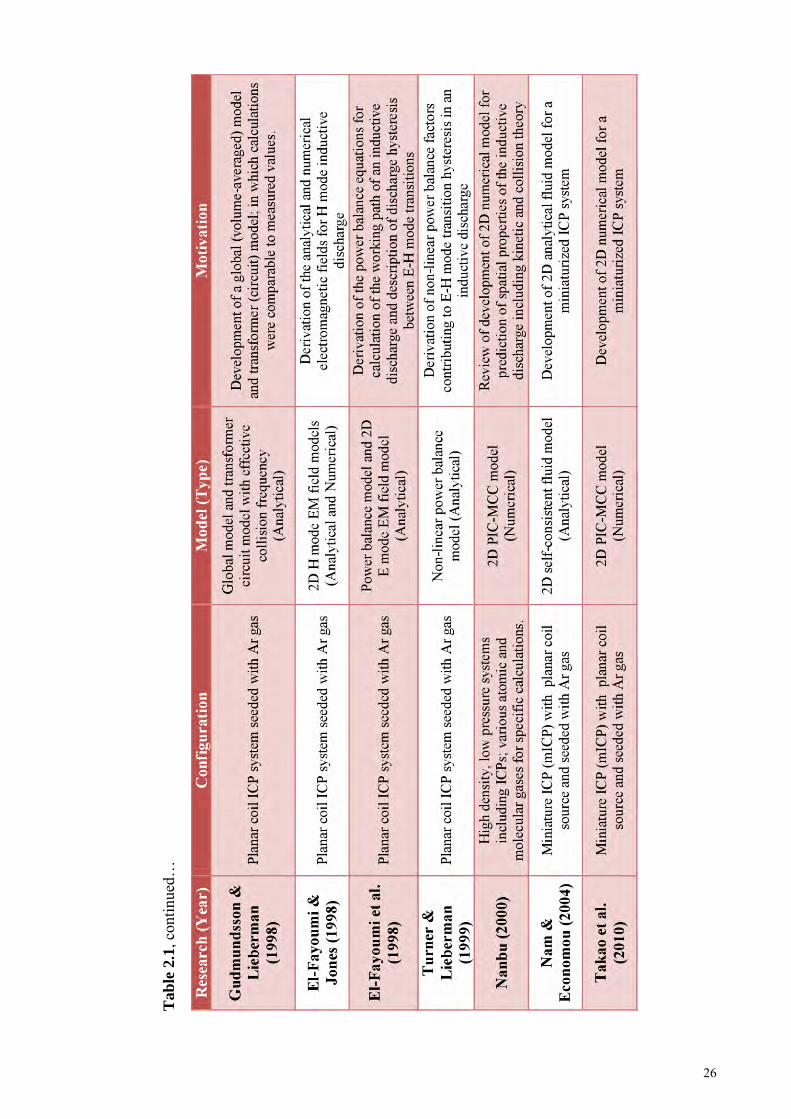
26

Tab

le 2

.1, c

ontin

ued…

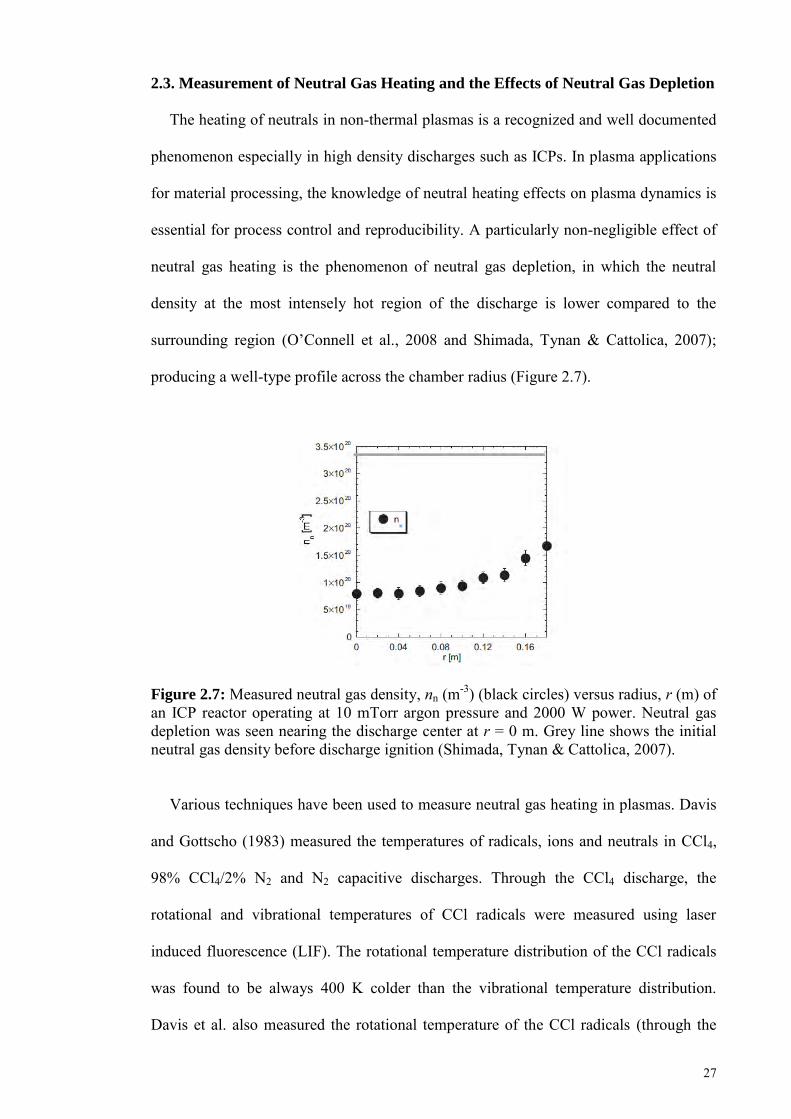
27

2.3. Measurement of Neutral Gas Heating and the Effects of Neutral Gas Depletion

The heating of neutrals in non-thermal plasmas is a recognized and well documented

phenomenon especially in high density discharges such as ICPs. In plasma applications

for material processing, the knowledge of neutral heating effects on plasma dynamics is

essential for process control and reproducibility. A particularly non-negligible effect of

neutral gas heating is the phenomenon of neutral gas depletion, in which the neutral

density at the most intensely hot region of the discharge is lower compared to the

surrounding region (O’Connell et al., 2008 and Shimada, Tynan & Cattolica, 2007);

producing a well-type profile across the chamber radius (Figure 2.7).

Figure 2.7: Measured neutral gas density, nn (m-3) (black circles) versus radius, r (m) of an ICP reactor operating at 10 mTorr argon pressure and 2000 W power. Neutral gas depletion was seen nearing the discharge center at r = 0 m. Grey line shows the initial neutral gas density before discharge ignition (Shimada, Tynan & Cattolica, 2007).

Various techniques have been used to measure neutral gas heating in plasmas. Davis

and Gottscho (1983) measured the temperatures of radicals, ions and neutrals in CCl4,

98% CCl4/2% N2 and N2 capacitive discharges. Through the CCl4 discharge, the

rotational and vibrational temperatures of CCl radicals were measured using laser

induced fluorescence (LIF). The rotational temperature distribution of the CCl radicals

was found to be always 400 K colder than the vibrational temperature distribution.

Davis et al. also measured the rotational temperature of the CCl radicals (through the

28

98% CCl4/2% N2 discharge) and N2 ions and neutrals (through the N2 discharge) using

the then novel technique of actinometry optical emission spectroscopy (AOES).

Comparisons between measured rotational temperatures for LIF and AOES were of

general agreement, however, AOES was found to be less viable when measurements

were made close to surfaces. At 19 mm axial distance from the lower chamber

electrode, the measured rotational temperatures for CCl radicals were 535 ± 25 K and

570 ± 30 K for LIF and AOES techniques, respectively

In 1987, Wormhoudt, Stanton, Richards and Sawin (1987) first introduced the use of

a tunable diode laser technique, i.e., tunable diode laser absorption spectroscopy

(TDLAS), to measure the neutral gas temperatures and atomic chlorine concentrations

in a chlorine (Cl2) glow discharge. The infrared transition used for measurement was

between the 2P1/2←2P3/2 spin orbit levels and occurred at 11.33 m wavelength. The

measured atomic chlorine translational temperature was 770 ± 100 K and was consistent

with measured rotational temperature found via AOES with nitrogen seed gas (95%

chlorine/5% nitrogen). Atomic chlorine concentration was shown to increase with

power (0-100 W) and pressure (200-800 mTorr) with the measured chlorine fractions in

the discharge being between 3-8% or (1.8-6.6)×1014 cm-3.

Hopwood and Asmussen (1991) measured the neutral gas temperatures in a 2.45

GHz, multipolar electron cyclotron resonance plasma source seeded with argon and

helium gases. Spectroscopic equipment which included an optical fiber probe, a Fabry-

Perot interferometer, a ramp generator, a photomultiplier tube and a monochromator

were used for this purpose. The argon and helium emission line profiles at 549.6 nm and

501.6 nm, respectively were measured and deconvolved with instrumental broadening

which was determined using the 480.7 nm emission of a 150 W, 0.67 mTorr and 10

29

sccm xenon ECR discharge. The effects of Zeeman splitting were also compensated in

the calculation to reveal constant Doppler broadening (widths) across the radius of the

plasma. Neutral gas heating of argon at 0.77 mTorr was found to increase from 300 K to

500 K when microwave power was increased from 80 to 330 W. Both helium and argon

neutral gas temperatures were shown to decrease as the neutral mean path increases

which, according to Hopwood et al. indicates that the gases may be heated by ion-

neutral collisional processes.

In a theoretical study, Fruchtman et al. (2005) investigated the impact of neutral gas

depletion in the enhancement of plasma transport by self-consistently solving the

pressure balance equations of plasma and neutral gas. Several parameters, including

electron temperature, rate of ionization and plasma density were also derived

analytically and visualized. It was found that the occurrence of neutral depletion in

simulation also lead to non-linear enhancement of plasma transport. This was attributed

to increased ionization and energy coupling in the region of interest. The enhancement

of plasma transport also lead to unexpected decrease in plasma density despite increase

in plasma power. In 2007, Liard et al. (2007) further extended the 2005 Fruchtman

model by self consistently incorporating the effects of neutral gas heating. With neutral

gas heating, stronger depletion was observed due to enhanced plasma transport to the

walls, i.e., larger plasma flux leaving the discharge at a given plasma density.

Also in 2005, Abdel-Rahman et al. used the Abel inversion of Fulcher line intensities

from OES to measure the phase and space resolved rotational temperatures of a

hydrogen, planar coil RF ICP with the consideration of cascading effects of higher level

molecular transitions. The rotational temperatures for different input powers and

operational modes of the discharge were characterized and compared at the pressure of

30

15 Pa. Cross-checking with linewidth measurements of translational (i.e., neutral gas)

temperature showed agreement. With the inclusion of cascading, it was found that

neutral gas temperatures within the coil axis could reach up to 650 K for the input

power of 350 W. Changes in these elevated temperatures were small throughout the r.f.

cycle; especially in comparison to an r.f. capacitively coupled plasma.

Shimada, Tynan and Cattolica (2007) measured the radial neutral gas temperature,

electron density, neutral gas pressure and total gas pressure profiles for pure N2,

He/5%N2 and Ar/5%N2 plasmas in an ICP reactor at ≤10 mTorr pressure. A radial

optical probe with a small light dump was used to measure the radial neutral gas

temperature via AOES. From measurements, a significant rise of neutral gas

temperature from room temperature, i.e., 600-900 K was observed for the three cases.

Neutral gas density at the central region of the chamber was found to be reduced by the

factor of 2-4 in the presence of the plasma (Figure 2.7). This depletion of neutrals was

attributed by Shimada et al. to the electron pressure in high density plasma which was

comparable to neutral gas pressure. Also in high density plasmas, the effects of neutral

gas heating become significant and affect neutral gas density. By correcting the effects

of thermal transpiration (which was neglected in previously published results, i.e.,

Tynan, 1999 and Yun, Taylor and Tynan, 2000) Shimada et al. found that the measured

total gas pressure remained uniform across the chamber radius despite variations in

neutral gas pressure.

O’Connell et al. (2008) investigated the neutral gas depletion mechanism in an

inductively coupled, magnetic neutral loop argon plasma at different pressure regimes.

In a magnetic neutral loop configuration, the inductive coil is designed to create a

neutral field region in which the plasma is generated; providing higher plasma

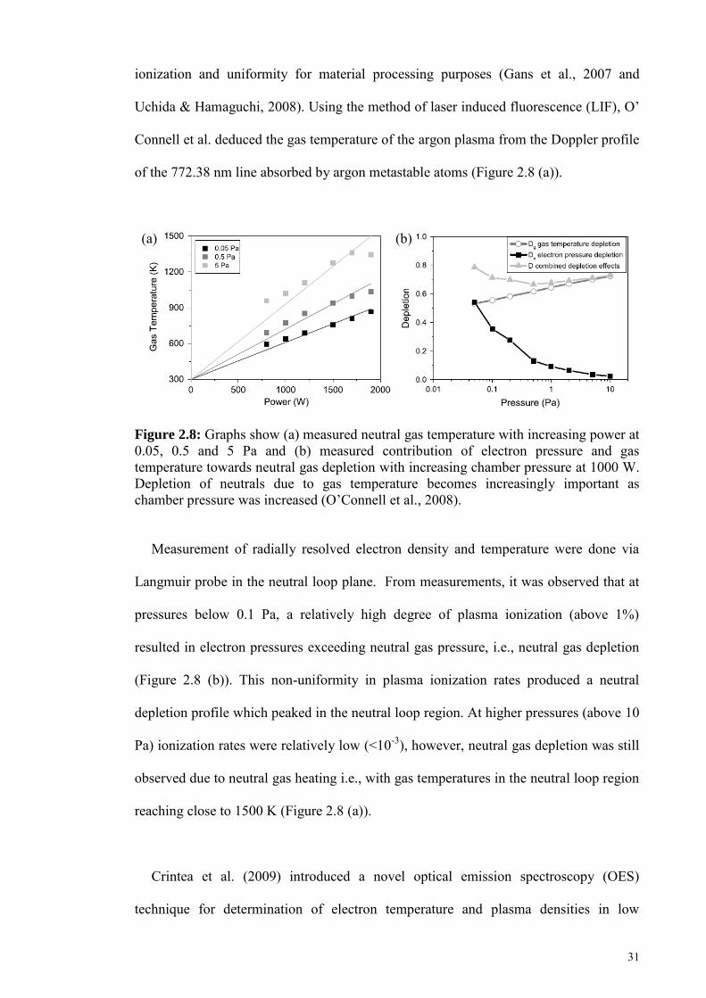
31

ionization and uniformity for material processing purposes (Gans et al., 2007 and

Uchida & Hamaguchi, 2008). Using the method of laser induced fluorescence (LIF), O’

Connell et al. deduced the gas temperature of the argon plasma from the Doppler profile

of the 772.38 nm line absorbed by argon metastable atoms (Figure 2.8 (a)).

Figure 2.8: Graphs show (a) measured neutral gas temperature with increasing power at 0.05, 0.5 and 5 Pa and (b) measured contribution of electron pressure and gas temperature towards neutral gas depletion with increasing chamber pressure at 1000 W. Depletion of neutrals due to gas temperature becomes increasingly important as chamber pressure was increased (O’Connell et al., 2008).

Measurement of radially resolved electron density and temperature were done via

Langmuir probe in the neutral loop plane. From measurements, it was observed that at

pressures below 0.1 Pa, a relatively high degree of plasma ionization (above 1%)

resulted in electron pressures exceeding neutral gas pressure, i.e., neutral gas depletion

(Figure 2.8 (b)). This non-uniformity in plasma ionization rates produced a neutral

depletion profile which peaked in the neutral loop region. At higher pressures (above 10

Pa) ionization rates were relatively low (<10-3), however, neutral gas depletion was still

observed due to neutral gas heating i.e., with gas temperatures in the neutral loop region

reaching close to 1500 K (Figure 2.8 (a)).

Crintea et al. (2009) introduced a novel optical emission spectroscopy (OES)

technique for determination of electron temperature and plasma densities in low

(a) (b)

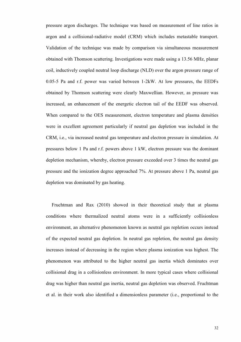
32

pressure argon discharges. The technique was based on measurement of line ratios in

argon and a collisional-radiative model (CRM) which includes metastable transport.

Validation of the technique was made by comparison via simultaneous measurement

obtained with Thomson scattering. Investigations were made using a 13.56 MHz, planar

coil, inductively coupled neutral loop discharge (NLD) over the argon pressure range of

0.05-5 Pa and r.f. power was varied between 1-2kW. At low pressures, the EEDFs

obtained by Thomson scattering were clearly Maxwellian. However, as pressure was

increased, an enhancement of the energetic electron tail of the EEDF was observed.

When compared to the OES measurement, electron temperature and plasma densities

were in excellent agreement particularly if neutral gas depletion was included in the

CRM, i.e., via increased neutral gas temperature and electron pressure in simulation. At

pressures below 1 Pa and r.f. powers above 1 kW, electron pressure was the dominant

depletion mechanism, whereby, electron pressure exceeded over 3 times the neutral gas

pressure and the ionization degree approached 7%. At pressure above 1 Pa, neutral gas

depletion was dominated by gas heating.

Fruchtman and Rax (2010) showed in their theoretical study that at plasma

conditions where thermalized neutral atoms were in a sufficiently collisionless

environment, an alternative phenomenon known as neutral gas repletion occurs instead

of the expected neutral gas depletion. In neutral gas repletion, the neutral gas density

increases instead of decreasing in the region where plasma ionization was highest. The

phenomenon was attributed to the higher neutral gas inertia which dominates over

collisional drag in a collisionless environment. In more typical cases where collisional

drag was higher than neutral gas inertia, neutral gas depletion was observed. Fruchtman

et al. in their work also identified a dimensionless parameter (i.e., proportional to the

33

ratio of plasma density and neutral gas density) that if larger or smaller than a critical

value was able to predict the occurrence of neutral repletion or depletion.

Song, Lee and Chung (2011) characterized the properties of a low pressure,

inductively coupled nitrogen-argon plasma using a combination of Langmuir probe and

AOES. The plasma was characterized at the pressure range of 1-30 mTorr and applied

r.f. power of 200-600 W. The actinometer used for AOES measurements was argon gas.

Electron energy probability function, electron density and electron temperature were

measured using an r.f. compensated Langmuir probe. The percentage of argon gas was

varied between 5%-80% and its effects on plasma density, electron temperature and the

dissociation fraction of nitrogen were observed. From experiments, it was found that as

the percentage of argon increased, the dissociation fraction of nitrogen also increased.

This was attributed to the increase in Penning excitation of the nitrogen atoms and the

Penning dissociation of nitrogen molecules due to increased presence of argon

metastables. Also, with increased argon percentage, the electron density was found to

increase and electron temperature to slightly decrease. Song et al. further calculated the

rotational and vibrational temperatures of +2N and N2 using the +

2N first negative system

2 2( ') ( ")u gB v X v and N2 second positive system 3 3( ') ( ")u gC v B v from

the molecular optical emission spectrum wavelength of 300-400 nm. The rotational

temperatures and vibrational temperatures at 1.4 mTorr pressure were derived to be

between 300-500 K and 8500-16500 K, respectively; with both values increasing with

argon percentage.

Li et al. (2011) investigated the dependence of neutral gas temperature on gas

pressure and r.f. power for argon and nitrogen inductively coupled plasmas using

actinometry optical emission spectroscopy (AOES). For the argon plasma, 5% nitrogen

34

gas was added to the total gas flow as an actinometer. The highest neutral gas

temperature measured for argon plasma was 1850 K at 1 Torr pressure and 600 W r.f.

power (Figure 2.9 (a)).

Figure 2.9: Measured neutral gas temperature versus (a) discharge power and (b) logarithm of pressure for an argon discharge using AOES. The highest neutral gas temperature obtained was 1850 K at 600 W and 1 Torr (Li et al., 2011).

The measured neutral gas temperature for argon (at H mode) was observed to vary

almost linearly with the logarithm of gas pressure (2 mTorr-1 Torr) but vary only

slightly within the r.f. power range (100-600 W) (Figure 2.9 (b)). E to H mode transition

occurred during the increase of gas pressure for the nitrogen plasma which resulted in

the sudden increase of measured values of neutral gas temperature. However, once in H

mode, neutral gas temperatures for nitrogen plasma varied linearly with pressure as seen

in argon plasma.

(a) (b)

35

CHAPTER 3: METHODOLOGY

3.0. Experimental Setup

A cylindrical stainless steel chamber of 0.29 m diameter and 0.30 m height was used

to generate the plasma for experiments (Figure 3.1). A 0.20 m diameter and 0.01 m

thick quartz dielectric plate is placed at the bottom of the chamber to allow transmission

of the fields from the source. A total of twelve NW50 ports (four ports at each of the

three levels) are located at the sides of the chamber for insertion of probes, vacuum

pump fittings and gas inlet fittings. The chamber was pumped down using a KYKY

FB450A turbo-molecular pump backed with an Edwards E2M18 rotary pump. A 6 turn

planar coil of 0.09 m diameter is connected to a T&C Power Conversion AG0613 13.56

MHz 600 W r.f. power supply and is used to generate the plasma. A 7:1 step-down

transformer was used to reduce the 50 source impedance to the range of the plasma

impedance (~1 ) which was fine tuned using a variable air capacitor to match the

plasma impedance. The primary discharge gas for the experiments, i.e., pure argon

(99.999%) was seeded through a molecular sieve (to remove moisture) before being

introduced into the system. The gas flow is controlled by two Dwyer GFC-2014 mass

flow controllers. Gas pressure measurements are made using an APG100-XLC Pirani

gauge. Chamber pressure was set by adjusting the flow rate of the mass flow controllers.

For actinometrical measurement of neutral gas temperature, a secondary gas, nitrogen is

added to the plasma in minuscule amounts (<5%). This gas is also flowed through an

additional direct reading flow meter (Gilmont, EW-03232-23) and a series of needle

valves for finer adjustment of the amount required.

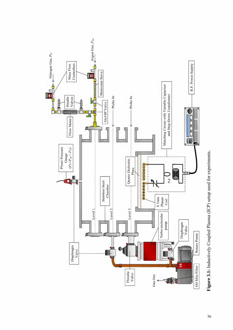
36

Fig

ure

3.1

: In

duct

ivel

y C

oupl

ed P

lasm

a (I

CP)

setu

p us

ed fo

r exp

erim

ents

.

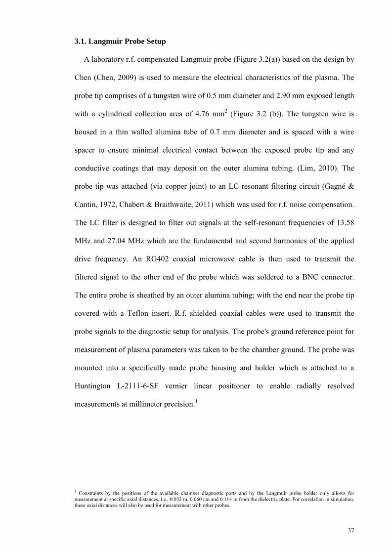
37

3.1. Langmuir Probe Setup

A laboratory r.f. compensated Langmuir probe (Figure 3.2(a)) based on the design by

Chen (Chen, 2009) is used to measure the electrical characteristics of the plasma. The

probe tip comprises of a tungsten wire of 0.5 mm diameter and 2.90 mm exposed length

with a cylindrical collection area of 4.76 mm2 (Figure 3.2 (b)). The tungsten wire is

housed in a thin walled alumina tube of 0.7 mm diameter and is spaced with a wire

spacer to ensure minimal electrical contact between the exposed probe tip and any

conductive coatings that may deposit on the outer alumina tubing. (Lim, 2010). The

probe tip was attached (via copper joint) to an LC resonant filtering circuit (Gagné &

Cantin, 1972, Chabert & Braithwaite, 2011) which was used for r.f. noise compensation.

The LC filter is designed to filter out signals at the self-resonant frequencies of 13.58

MHz and 27.04 MHz which are the fundamental and second harmonics of the applied

drive frequency. An RG402 coaxial microwave cable is then used to transmit the

filtered signal to the other end of the probe which was soldered to a BNC connector.

The entire probe is sheathed by an outer alumina tubing; with the end near the probe tip

covered with a Teflon insert. R.f. shielded coaxial cables were used to transmit the

probe signals to the diagnostic setup for analysis. The probe's ground reference point for

measurement of plasma parameters was taken to be the chamber ground. The probe was

mounted into a specifically made probe housing and holder which is attached to a

Huntington L-2111-6-SF vernier linear positioner to enable radially resolved

measurements at millimeter precision.1

1 Constraints by the positions of the available chamber diagnostic ports and by the Langmuir probe holder only allows for measurement at specific axial distances, i.e., 0.032 m, 0.060 cm and 0.114 m from the dielectric plate. For correlation in simulation, these axial distances will also be used for measurement with other probes.

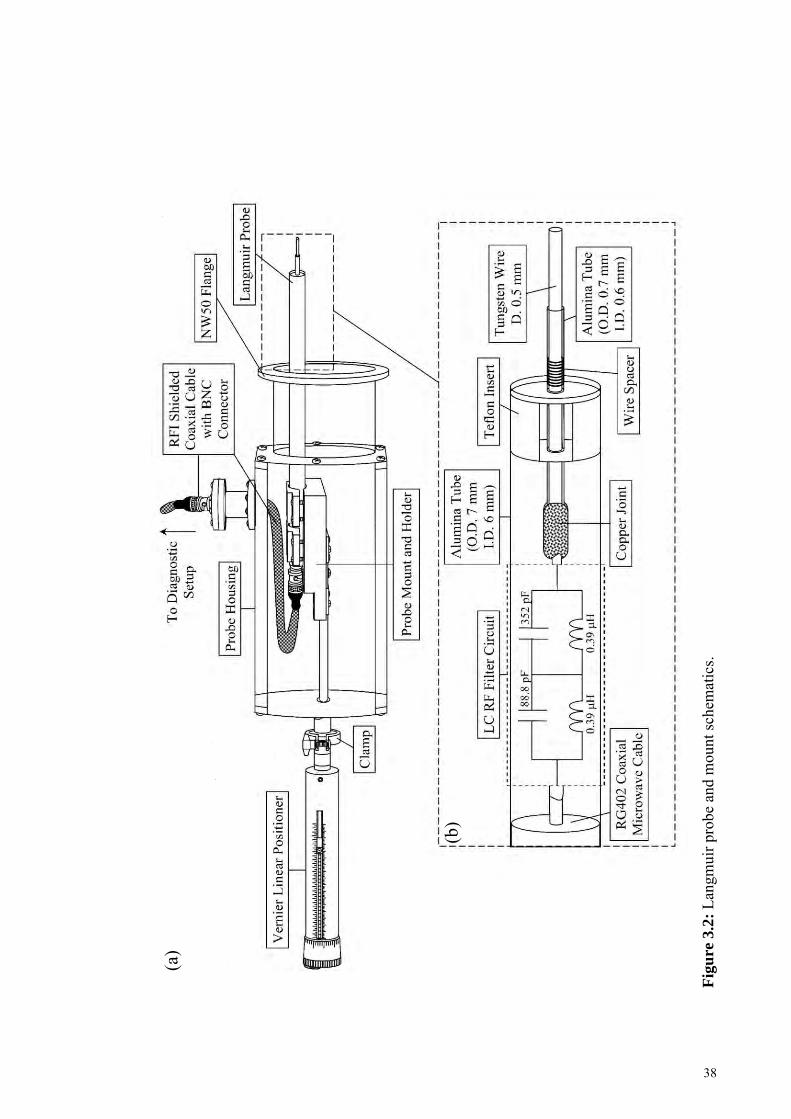
38

Fig

ure

3.2

: La

ngm

uir p

robe

and

mou

nt sc

hem

atic

s.

(a)

(b)

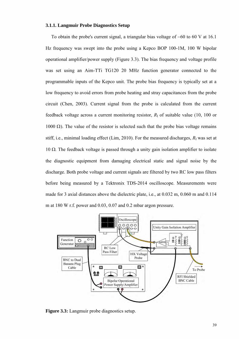
39

3.1.1. Langmuir Probe Diagnostics Setup

To obtain the probe's current signal, a triangular bias voltage of 60 to 60 V at 16.1

Hz frequency was swept into the probe using a Kepco BOP 100-1M, 100 W bipolar

operational amplifier/power supply (Figure 3.3). The bias frequency and voltage profile

was set using an Aim-TTi TG120 20 MHz function generator connected to the

programmable inputs of the Kepco unit. The probe bias frequency is typically set at a

low frequency to avoid errors from probe heating and stray capacitances from the probe

circuit (Chen, 2003). Current signal from the probe is calculated from the current

feedback voltage across a current monitoring resistor, RI of suitable value (10, 100 or

1000 ). The value of the resistor is selected such that the probe bias voltage remains

stiff, i.e., minimal loading effect (Lim, 2010). For the measured discharges, RI was set at

10 The feedback voltage is passed through a unity gain isolation amplifier to isolate

the diagnostic equipment from damaging electrical static and signal noise by the

discharge. Both probe voltage and current signals are filtered by two RC low pass filters

before being measured by a Tektronix TDS-2014 oscilloscope. Measurements were

made for 3 axial distances above the dielectric plate, i.e., at 0.032 m, 0.060 m and 0.114

m at 180 W r.f. power and 0.03, 0.07 and 0.2 mbar argon pressure.

Figure 3.3: Langmuir probe diagnostics setup.

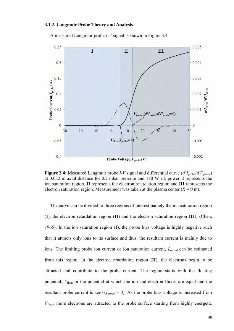
40

3.1.2. Langmuir Probe Theory and Analysis

A measured Langmuir probe I-V signal is shown in Figure 3.4.

Figure 3.4: Measured Langmuir probe I-V signal and differential curve (d2Iprobe/dV2probe)

at 0.032 m axial distance for 0.2 mbar pressure and 180 W r.f. power. I represents the ion saturation region, II represents the electron retardation region and III represents the electron saturation region. Measurement was taken at the plasma center (R = 0 m).

The curve can be divided to three regions of interest namely the ion saturation region

(I), the electron retardation region (II) and the electron saturation region (III) (Chen,

1965). In the ion saturation region (I), the probe bias voltage is highly negative such

that it attracts only ions to its surface and thus, the resultant current is mainly due to

ions. The limiting probe ion current or ion saturation current, Iion,sat can be estimated

from this region. In the electron retardation region (II), the electrons begin to be

attracted and contribute to the probe current. The region starts with the floating

potential, Vfloat or the potential at which the ion and electron fluxes are equal and the

resultant probe current is zero (Iprobe = 0). As the probe bias voltage is increased from

Vfloat, more electrons are attracted to the probe surface starting from highly energetic

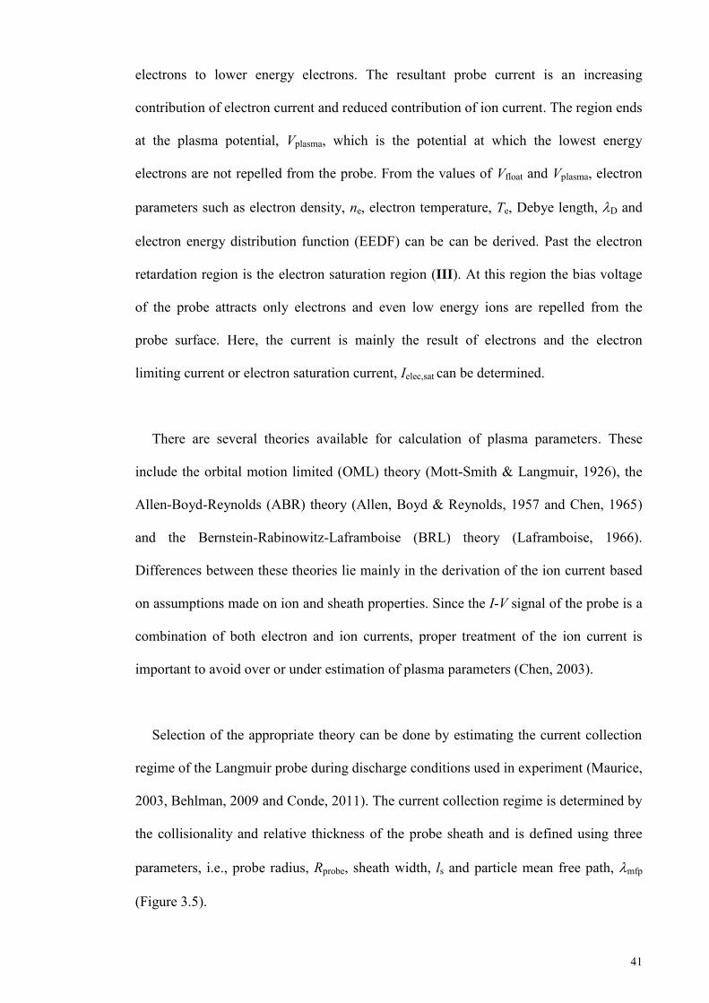
41

electrons to lower energy electrons. The resultant probe current is an increasing

contribution of electron current and reduced contribution of ion current. The region ends

at the plasma potential, Vplasma, which is the potential at which the lowest energy

electrons are not repelled from the probe. From the values of Vfloat and Vplasma, electron

parameters such as electron density, ne, electron temperature, Te, Debye length, D and

electron energy distribution function (EEDF) can be can be derived. Past the electron

retardation region is the electron saturation region (III). At this region the bias voltage

of the probe attracts only electrons and even low energy ions are repelled from the

probe surface. Here, the current is mainly the result of electrons and the electron

limiting current or electron saturation current, Ielec,sat can be determined.

There are several theories available for calculation of plasma parameters. These

include the orbital motion limited (OML) theory (Mott-Smith & Langmuir, 1926), the

Allen-Boyd-Reynolds (ABR) theory (Allen, Boyd & Reynolds, 1957 and Chen, 1965)

and the Bernstein-Rabinowitz-Laframboise (BRL) theory (Laframboise, 1966).

Differences between these theories lie mainly in the derivation of the ion current based

on assumptions made on ion and sheath properties. Since the I-V signal of the probe is a

combination of both electron and ion currents, proper treatment of the ion current is

important to avoid over or under estimation of plasma parameters (Chen, 2003).

Selection of the appropriate theory can be done by estimating the current collection

regime of the Langmuir probe during discharge conditions used in experiment (Maurice,

2003, Behlman, 2009 and Conde, 2011). The current collection regime is determined by

the collisionality and relative thickness of the probe sheath and is defined using three

parameters, i.e., probe radius, Rprobe, sheath width, ls and particle mean free path, mfp

(Figure 3.5).

42

Figure 3.5: The four different current collection regimes for a Langmuir probe (Maurice, 2003).

A thin or thick probe sheath regime is deduced by comparing the probe sheath

thickness, ls with the probe radius, Rprobe, i.e., ls << Rprobe and ls >> Rprobe for thin and

thick sheath, respectively. On the other hand, sheath collisionality in experiment

conditions can be determined by comparing ls to the mean free path, mfp of important

particle interactions near the probe sheath including electron-neutral mean free path, en

ion-neutral mean free path, in and ion-ion mean free path, ii. If ls < mfp, the sheath is

considered to be collisonless, else if ls > mfp, the sheath is seen as collisional. The probe

sheath thickness, ls for regime determination can be generally approximated by using

Child-Langmuir relation (Lieberman & Lichtenberg, 2005 and Chabert & Braithwaite,

2011), i.e.,

43

3/4

ss D

e

.VlT

(3.1.1)

Here, Vs is the potential difference of the plasma sheath in V and Te is the electron

temperature in eV. The Debye length,D (in m) is given by,

eD

e, cm

7.43 ,Tn

(3.1.2)

where, ne, cm is the electron density in cm-3. To estimate the mean free paths en, in and

ii, the following equations were used (Lieberman & Lichtenberg, 2005 and Maurice,

2003),

eng en

1 ,n

(3.1.3)

ing in

1 ,n

(3.1.4)

and

17 2i

iie

2.8 10 ,ln

Tn

(3.1.5)

where, ng is the neutral gas density in m-3, en and in are the electron-neutral total

collision cross section and ion-neutral scattering cross section, respectively in m2, Ti is

the ion temperature in eV, ne is the electron density in m-3 and ln is the Coulomb

logarithm. ng is calculated by using ideal gas law, i.e.,

.nB

g TkPn (3.1.6)

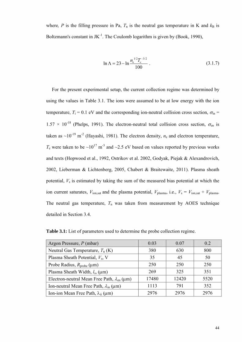
44

where, P is the filling pressure in Pa, Tn is the neutral gas temperature in K and kB is

Boltzmann's constant in JK-1. The Coulomb logarithm is given by (Book, 1990),

1/2 3/2eln 23 ln .100

en T

(3.1.7)

For the present experimental setup, the current collection regime was determined by

using the values in Table 3.1. The ions were assumed to be at low energy with the ion

temperature, Ti = 0.1 eV and the corresponding ion-neutral collision cross section, in =

1.57 × 10-18 (Phelps, 1991). The electron-neutral total collision cross section, en is

taken as ~10-19 m-2 (Hayashi, 1981). The electron density, ne and electron temperature,

Te were taken to be ~1017 m-3 and ~2.5 eV based on values reported by previous works

and texts (Hopwood et al., 1992, Ostrikov et al. 2002, Godyak, Piejak & Alexandrovich,

2002, Lieberman & Lichtenberg, 2005, Chabert & Braitewaite, 2011). Plasma sheath

potential, Vs is estimated by taking the sum of the measured bias potential at which the

ion current saturates, Vion,sat and the plasma potential, Vplasma, i.e., Vs = Vion,sat + Vplasma.

The neutral gas temperature, Tn was taken from measurement by AOES technique

detailed in Section 3.4.

Table 3.1: List of parameters used to determine the probe collection regime.

Argon Pressure, P (mbar) 0.03 0.07 0.2 Neutral Gas Temperature, Tn (K) 380 630 800 Plasma Sheath Potential, Vs, V 35 45 50 Probe Radius, Rprobe (m) 250 250 250 Plasma Sheath Width, ls, (m) 269 325 351 Electron-neutral Mean Free Path, en (m) 17480 12420 5520 Ion-neutral Mean Free Path, in (m) 1113 791 352 Ion-ion Mean Free Path, ii (m) 2976 2976 2976

45

For the range of pressures used in experiment, the probe sheath was found to be thick

(ls > Rprobe) and collisionless (ls < mfp). Based on the probe collection regime, the orbital

motion limited (OML) theory was found to be most suitable for calculation of plasma

parameters. The plasma potential, Vp is first determined by taking the crossing point of

the second derivative of the probe I-V curve with zero, i.e. d2I/dV2 = 0. This technique

allows for more accurate determination of Vp without the ambiguity of approximate

methods. The floating potential, Vf is determined by taking the potential at which I = 0.

As previously mentioned, probe current, Iprobe, is the sum of the ion current, Iion and the

electron current, Ielec, i.e., Iprobe = Iion + Ielec. Thus, before calculation of electron

parameters, Iion has to be first subtracted from Iprobe to obtain Ielec across the signal range.

A linear extrapolation from the ion saturation region is used as the estimation of Iion for

subtraction (Chen, 2003).

The electron temperature, Te and electron density, ne is subsequently calculated using

the following equations (Maurice, 2003 and Chen, 2009):

p

fe

ee p

( )

( )

V

VI V dV

TI V

(3.1.8)

and

1/2e p e

e 2p B e

( ) 2 .I V mn

A e k T

(3.1.9)

Here, Ie(V) and Ie(Vp) are the electron current and the electron current at the plasma

potential, respectively, in A. Ap is the probe collection area in m2, me is the mass of

electrons in kg, Te is the electron temperature in K and e is the electronic charge in C.

The electron energy distribution function, f () or EEDF provides important information

46

of the energy distribution of electrons at a particular position from which the collisional

processes involving the particles can be deduced. is the electron energy between V = 0

to V = Vp, in eV. Assuming that in the electron retardation region, the second derivative

of the I-V curve is equal to the second derivative of the electron current (i.e., the second

derivative of the ion current is negligible), the EEDF can be calculated by using the

Druyvesteyn expression (Godyak, Piejak & Alexandrovich, 2002 and Magnus &

Gudmundsson, 2008),

1/2e

e3/2p

2( ) 2 .If m Ve A

(3.1.10)

The EEDF can also alternately be used to calculate the electron density, ne (m-3) and

effective electron temperature, Te,eff (eV) using,

0e )( dfn (3.1.11)

and

e,eff2 .3

T

(3.1.12)

Here, <> is the average electron energy in eV which can be found by using,

0

e

( ) .

f dn

(3.1.13)

47

To calculate plasma parameters from the current-voltage characteristics a MATLAB

code was written (see Appendix A). The electron density and electron temperature were

calculated using both Maxwellian distribution assumption and EEDF methods.

3.2. Magnetic Probe Setup

Electrostatic noise compensated, center-tapped, axial and radial magnetic probes

(Chakrabarty, 2006) were constructed to measure the radially resolved magnetic field

distributions in the plasma (Figure 3.6(a)). Each probe (pick-up coil) was made using

two 0.25 mm diameter copper wires which were wound together and grounded at

opposing ends (Figure 3.6 (b)) on a small quartz tube of 2 mm in diameter and 5 mm

length. The ends of the windings are twisted and the wires are run through a 48 cm long

copper tube of 3.3 mm diameter which is attached to a cylindrical copper housing that

holds two BNC connectors. The copper housing and tubing are ensured to be properly

sealed together with copper foil tape to minimize pickup of stray r.f. signals. The ends

of the wires were soldered to two BNC connectors. The axial probe solenoid is

perpendicular to the copper tube (z-direction), whereas the radial probe solenoid is

parallel (r-direction), i.e., (Figure 3.6 (c)). A port attachment with two fixed Pyrex tubes

was fitted to the chamber for shielding of the magnetic probe during radially resolved

measurements of the plasma. Measurements were made at 0.032 m and 0.060 m axial

distances above the dielectric plate for 180 W r.f. power and 0.03, 0.07 and 0.2 mbar

argon pressures. Simultaneous measurements of coil current and voltage were also made

during the measurement of the fields with the respective probes (probe details in Section

3.3). Results were collected via Tektronix TDS-2014 oscilloscope.

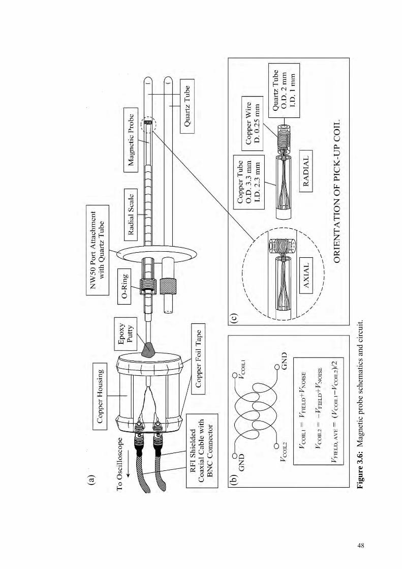
48

Fig

ure

3.6

: M

agne

tic p

robe

sche

mat

ics a

nd c

ircui

t.

(b)

(c

)

(a)

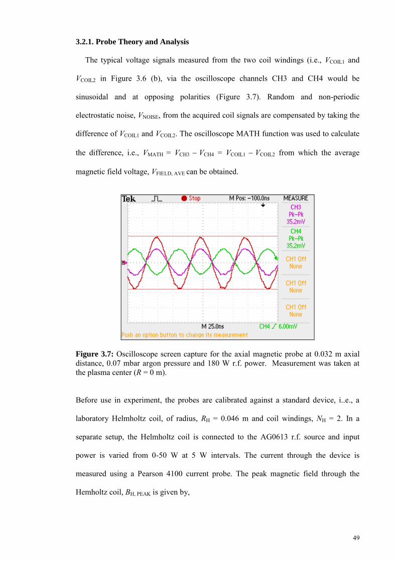
49

3.2.1. Probe Theory and Analysis

The typical voltage signals measured from the two coil windings (i.e., VCOIL1 and

VCOIL2 in Figure 3.6 (b), via the oscilloscope channels CH3 and CH4 would be

sinusoidal and at opposing polarities (Figure 3.7). Random and non-periodic

electrostatic noise, VNOISE, from the acquired coil signals are compensated by taking the

difference of VCOIL1 and VCOIL2. The oscilloscope MATH function was used to calculate

the difference, i.e., VMATH = VCH3 VCH4 = VCOIL1 VCOIL2 from which the average

magnetic field voltage, VFIELD, AVE can be obtained.

Figure 3.7: Oscilloscope screen capture for the axial magnetic probe at 0.032 m axial distance, 0.07 mbar argon pressure and 180 W r.f. power. Measurement was taken at the plasma center (R = 0 m).

Before use in experiment, the probes are calibrated against a standard device, i..e., a

laboratory Helmholtz coil, of radius, RH = 0.046 m and coil windings, NH = 2. In a

separate setup, the Helmholtz coil is connected to the AG0613 r.f. source and input

power is varied from 0-50 W at 5 W intervals. The current through the device is

measured using a Pearson 4100 current probe. The peak magnetic field through the

Hemholtz coil, BH, PEAK is given by,

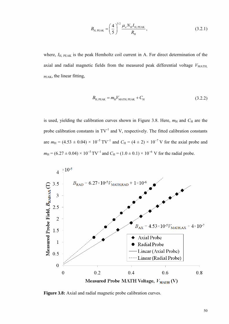
50

3/2H H, PEAK

H, PEAKH

4 ,5

oN IB

R

(3.2.1)

where, IH, PEAK is the peak Hemholtz coil current in A. For direct determination of the

axial and radial magnetic fields from the measured peak differential voltage VMATH,

PEAK, the linear fitting,

H, PEAK H MATH, PEAK HB m V C (3.2.2)

is used, yielding the calibration curves shown in Figure 3.8. Here, mH and CH are the

probe calibration constants in TV-1 and V, respectively. The fitted calibration constants

are mH = (4.53 ± 0.04) × 105 TV1 and CH = (4 ± 2) × 107 V for the axial probe and

mH = (6.27 ± 0.04) × 105 TV1 and CH = (1.0 ± 0.1) × 106 V for the radial probe.

Figure 3.8: Axial and radial magnetic probe calibration curves.

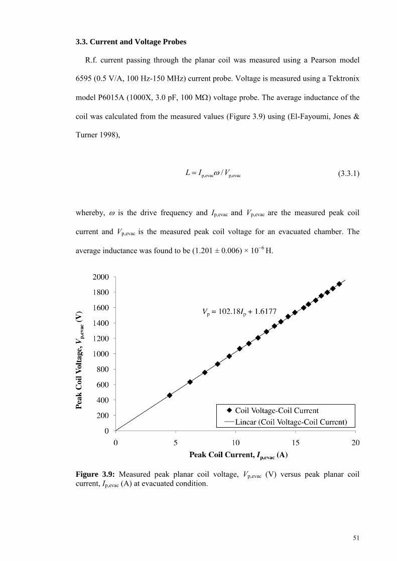
51

3.3. Current and Voltage Probes

R.f. current passing through the planar coil was measured using a Pearson model

6595 (0.5 V/A, 100 Hz-150 MHz) current probe. Voltage is measured using a Tektronix

model P6015A (1000X, 3.0 pF, 100 M voltage probe. The average inductance of the

coil was calculated from the measured values (Figure 3.9) using (El-Fayoumi, Jones &

Turner 1998),

p,evac p,evac/L I V (3.3.1)

whereby, is the drive frequency and Ip,evac and Vp,evac are the measured peak coil

current and Vp,evac is the measured peak coil voltage for an evacuated chamber. The

average inductance was found to be (1.201 ± 0.006) × 106 H.

Figure 3.9: Measured peak planar coil voltage, Vp,evac (V) versus peak planar coil current, Ip,evac (A) at evacuated condition.

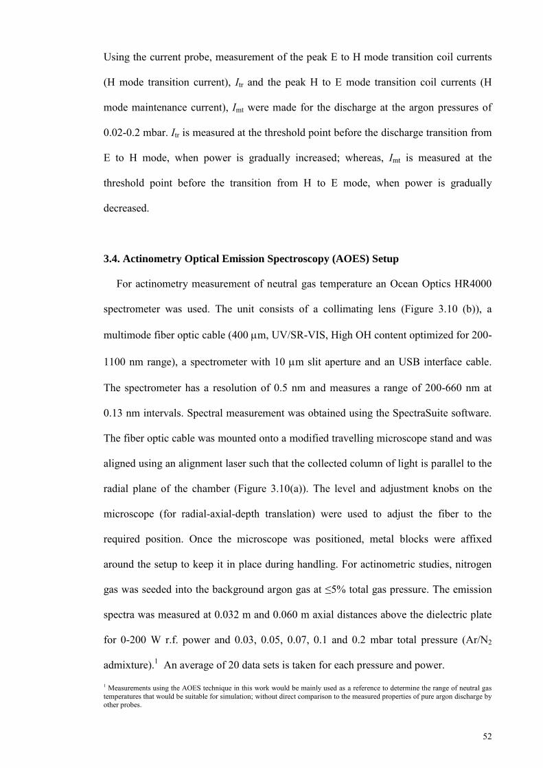
52

Using the current probe, measurement of the peak E to H mode transition coil currents

(H mode transition current), Itr and the peak H to E mode transition coil currents (H

mode maintenance current), Imt were made for the discharge at the argon pressures of

0.02-0.2 mbar. Itr is measured at the threshold point before the discharge transition from

E to H mode, when power is gradually increased; whereas, Imt is measured at the

threshold point before the transition from H to E mode, when power is gradually

decreased.

3.4. Actinometry Optical Emission Spectroscopy (AOES) Setup

For actinometry measurement of neutral gas temperature an Ocean Optics HR4000

spectrometer was used. The unit consists of a collimating lens (Figure 3.10 (b)), a

multimode fiber optic cable (400 m, UV/SR-VIS, High OH content optimized for 200-

1100 nm range), a spectrometer with 10 m slit aperture and an USB interface cable.

The spectrometer has a resolution of 0.5 nm and measures a range of 200-660 nm at

0.13 nm intervals. Spectral measurement was obtained using the SpectraSuite software.

The fiber optic cable was mounted onto a modified travelling microscope stand and was

aligned using an alignment laser such that the collected column of light is parallel to the

radial plane of the chamber (Figure 3.10(a)). The level and adjustment knobs on the

microscope (for radial-axial-depth translation) were used to adjust the fiber to the

required position. Once the microscope was positioned, metal blocks were affixed

around the setup to keep it in place during handling. For actinometric studies, nitrogen

gas was seeded into the background argon gas at ≤5% total gas pressure. The emission

spectra was measured at 0.032 m and 0.060 m axial distances above the dielectric plate

for 0-200 W r.f. power and 0.03, 0.05, 0.07, 0.1 and 0.2 mbar total pressure (Ar/N2

admixture).1 An average of 20 data sets is taken for each pressure and power.

1 Measurements using the AOES technique in this work would be mainly used as a reference to determine the range of neutral gas temperatures that would be suitable for simulation; without direct comparison to the measured properties of pure argon discharge by other probes.

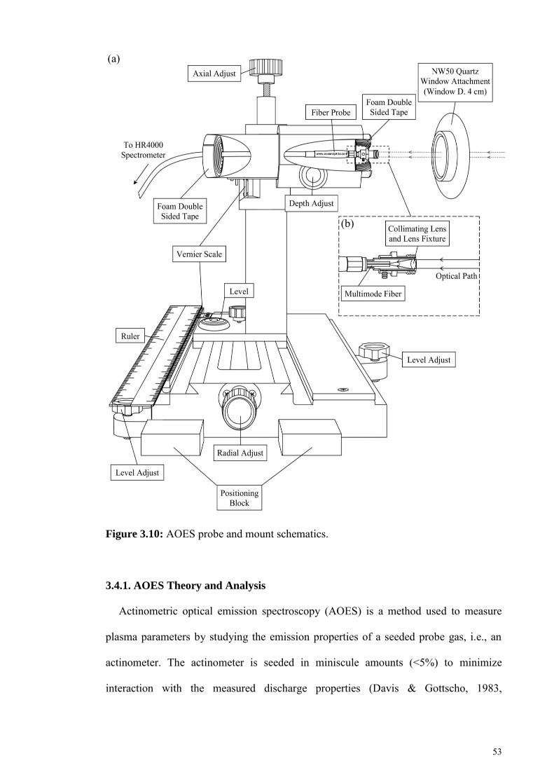
53

Figure 3.10: AOES probe and mount schematics.

3.4.1. AOES Theory and Analysis

Actinometric optical emission spectroscopy (AOES) is a method used to measure

plasma parameters by studying the emission properties of a seeded probe gas, i.e., an

actinometer. The actinometer is seeded in miniscule amounts (<5%) to minimize

interaction with the measured discharge properties (Davis & Gottscho, 1983,

(a)

(b)

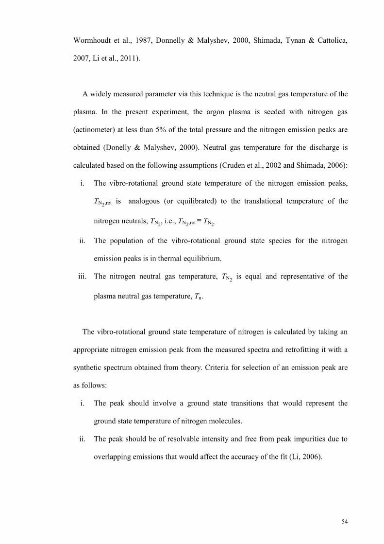
54

Wormhoudt et al., 1987, Donnelly & Malyshev, 2000, Shimada, Tynan & Cattolica,

2007, Li et al., 2011).

A widely measured parameter via this technique is the neutral gas temperature of the

plasma. In the present experiment, the argon plasma is seeded with nitrogen gas

(actinometer) at less than 5% of the total pressure and the nitrogen emission peaks are

obtained (Donelly & Malyshev, 2000). Neutral gas temperature for the discharge is

calculated based on the following assumptions (Cruden et al., 2002 and Shimada, 2006):

i. The vibro-rotational ground state temperature of the nitrogen emission peaks,

TN2,rot is analogous (or equilibrated) to the translational temperature of the

nitrogen neutrals, TN2, i.e., TN2,rot ≡ TN2.

ii. The population of the vibro-rotational ground state species for the nitrogen

emission peaks is in thermal equilibrium.

iii. The nitrogen neutral gas temperature, TN2 is equal and representative of the

plasma neutral gas temperature, Tn.

The vibro-rotational ground state temperature of nitrogen is calculated by taking an

appropriate nitrogen emission peak from the measured spectra and retrofitting it with a

synthetic spectrum obtained from theory. Criteria for selection of an emission peak are

as follows:

i. The peak should involve a ground state transitions that would represent the

ground state temperature of nitrogen molecules.

ii. The peak should be of resolvable intensity and free from peak impurities due to

overlapping emissions that would affect the accuracy of the fit (Li, 2006).

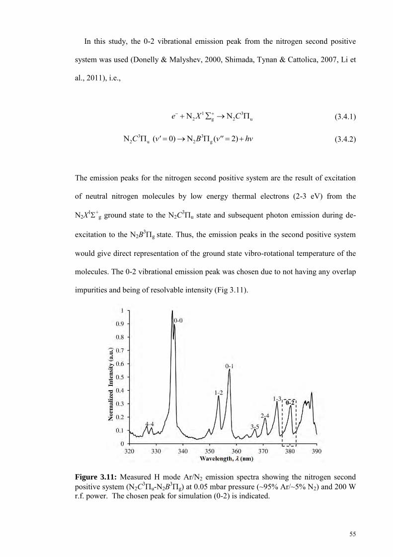
55

In this study, the 0-2 vibrational emission peak from the nitrogen second positive

system was used (Donelly & Malyshev, 2000, Shimada, Tynan & Cattolica, 2007, Li et

al., 2011), i.e.,

1 32 g 2 uN Ne X C (3.4.1)

3 32 u 2 gN ( 0) N ( 2)C v' B v'' hv (3.4.2)

The emission peaks for the nitrogen second positive system are the result of excitation

of neutral nitrogen molecules by low energy thermal electrons (2-3 eV) from the

N2X1

+g ground state to the N2C3

u state and subsequent photon emission during de-

excitation to the N2B3g state. Thus, the emission peaks in the second positive system

would give direct representation of the ground state vibro-rotational temperature of the

molecules. The 0-2 vibrational emission peak was chosen due to not having any overlap

impurities and being of resolvable intensity (Fig 3.11).

Figure 3.11: Measured H mode Ar/N2 emission spectra showing the nitrogen second positive system (N2C3

u-N2B3g) at 0.05 mbar pressure (~95% Ar/~5% N2) and 200 W

r.f. power. The chosen peak for simulation (0-2) is indicated.

56

To calculate the neutral gas temperature, the theoretical vibro-rotational spectral lines

have to be determined and matched with experimental measurement. There are 3 steps

involved (Shimada, 2006 and Li, 2006):

i. To calculate all possible quantum spectral line positions and intensities as

prescribed by atomic/molecular physics theory.

ii. To convolve the discrete spectral lines with instrumental broadening to form a

continuous spectrum similar to that of experimental measurement.

iii. To retrofit the continuous theoretical spectrum with measured experimental

spectrum using minimum chi squared (2) analysis by varying rotational

temperature (higher rotational temperature results in overall increased spectral

broadening) and finding the minimum 2 value.

The synthetic vibro-rotational nitrogen emission peak for fitting with experiment is

calculated using the atomic and molecular quantum theory found in Herzberg (1950),

Kovac (1969) and Hollas (2004). A vibrational emission peak for an electronic state

transition (e.g., 3 32 u 2 gN NC B ) is made up of many discretized rotational

emissions of which its line positions can be expressed as,

air

1( , , , ) ,( , , , )i

i

v v ' J J 'v v ' J J ' n

(3.4.3)

where, nair is the refractive index of air, i is the transitional vibro-rotational

wavenumber of the spectral line in cm-1, v is the vibrational quantum number and J is

the rotational quantum number. The notations ' and '' represent the upper and lower

transition states, respectively, i.e., for the 0-2 vibrational emission peak, the upper state

(N2C3u) vibrational quantum number, v' = 0 and the lower state (N2B3

g) vibrational

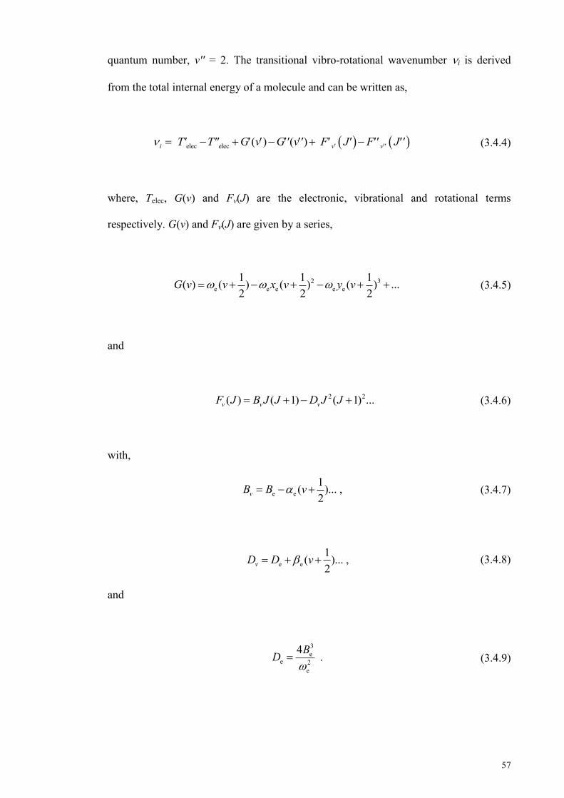
57

quantum number, v'' = 2. The transitional vibro-rotational wavenumber i is derived

from the total internal energy of a molecule and can be written as,

elec elec ( ) ( ) i v vT' T" G v G' v ' F J' F J ' (3.4.4)

where, Telec, G(v) and Fv(J) are the electronic, vibrational and rotational terms

respectively. G(v) and Fv(J) are given by a series,

2 3e e e e e

1 1 1( ) ( ) ( ) ( ) ... 2 2 2

G v v x v y v (3.4.5)

and

2 2( ) ( 1) ( 1) ... v v vF J B J J D J J (3.4.6)

with,

e e1( )... ,2vB B v (3.4.7)

e e1( )... ,2vD D v

(3.4.8)

and

3e

e 2e

4 .BD

(3.4.9)

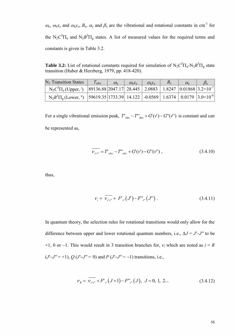
58

e, exe and eye, Be, e and e are the vibrational and rotational constants in cm-1 for

the N2C3u and N2B3

g states. A list of measured values for the required terms and

constants is given in Table 3.2.

Table 3.2: List of rotational constants required for simulation of N2C3

u-N2B3g state

transition (Huber & Herzberg, 1979, pp. 418-420).

N2 Transition States Telec e exe eye Be e e

N2C3u (Upper, ') 89136.88 2047.17 28.445 2.0883 1.8247 0.01868 3.2×10-7

N2B3g (Lower, '') 59619.35 1733.39 14.122 -0.0569 1.6374 0.0179 3.0×10-8

For a single vibrational emission peak, elec elec ( ) ( )T T ' G v G' v ' is constant and can

be represented as,

( ) ( ) ,v v elec elecT T ' G v G' v ' (3.4.10)

thus,

.i v v v vF J F ' J ' (3.4.11)

In quantum theory, the selection rules for rotational transitions would only allow for the

difference between upper and lower rotational quantum numbers, i.e., ΔJ = J'J'' to be

+1, 0 or 1. This would result in 3 transition branches for,i which are noted as i = R

(J'J'' = +1), Q (J'J'' = 0) and P (J'J'' = 1) transitions, i.e.,

1 , 0, 1, 2...R v v v vF J F ' J J (3.4.12)

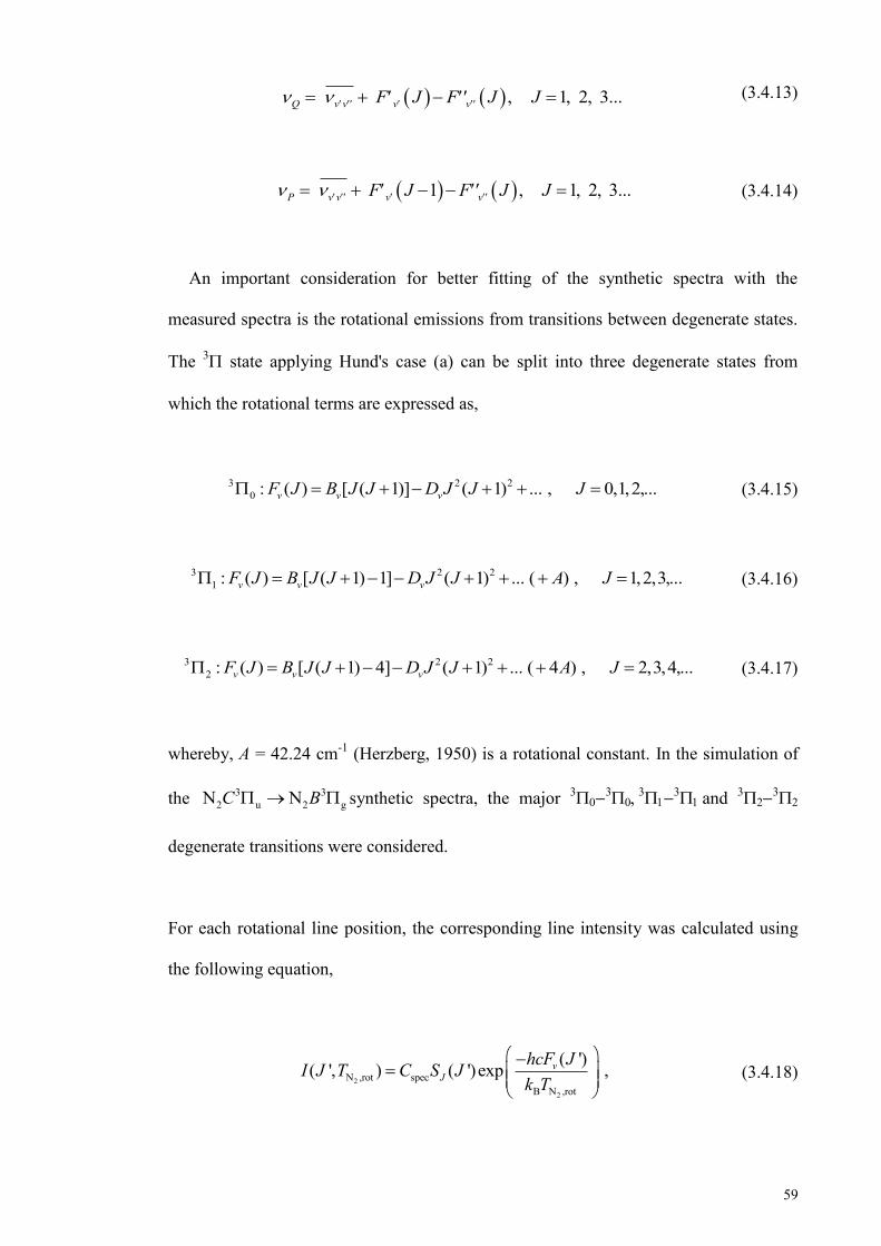
59

, 1, 2, 3...Q v v v vF J F ' J J (3.4.13)

1 , 1, 2, 3...P v v v vF J F ' J J

(3.4.14)

An important consideration for better fitting of the synthetic spectra with the

measured spectra is the rotational emissions from transitions between degenerate states.

The 3 state applying Hund's case (a) can be split into three degenerate states from

which the rotational terms are expressed as,

3 2 20 : ( ) [ ( 1)] ( 1) ... , 0,1,2,...v v vF J B J J D J J J (3.4.15)

3 2 2

1 : ( ) [ ( 1) 1] ( 1) ... ( ) , 1,2,3,...v v vF J B J J D J J A J

(3.4.16)

3 2 22 : ( ) [ ( 1) 4] ( 1) ... ( 4 ) , 2,3,4,...v v vF J B J J D J J A J

(3.4.17)

whereby, A = 42.24 cm-1 (Herzberg, 1950) is a rotational constant. In the simulation of

the 3 32 u 2 gN NC B synthetic spectra, the major 3

3

3

3and 3

3

degenerate transitions were considered.

For each rotational line position, the corresponding line intensity was calculated using

the following equation,

2

2

N ,rot specB N ,rot

( ')( ', ) ( ')exp ,vJ

hcF JI J T C S Jk T

(3.4.18)

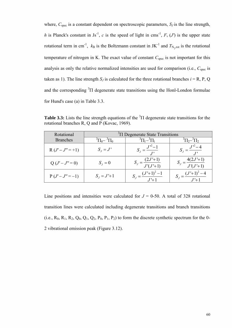
60

where, Cspec is a constant dependent on spectroscopic parameters, SJ is the line strength,

h is Planck's constant in Js-1, c is the speed of light in cms-1, Fv (J') is the upper state

rotational term in cm-1, kB is the Boltzmann constant in JK-1 and TN2,rot is the rotational

temperature of nitrogen in K. The exact value of constant Cspec is not important for this

analysis as only the relative normalized intensities are used for comparison (i.e., Cspec is

taken as 1). The line strength SJ is calculated for the three rotational branches i = R, P, Q

and the corresponding 3 degenerate state transitions using the Honl-London formulae

for Hund's case (a) in Table 3.3.

Table 3.3: Lists the line strength equations of the 3 degenerate state transitions for the rotational branches R, Q and P (Kovac, 1969).

Rotational Branches

3 Degenerate State Transitions 3

3

3

3

3

3

R (J' J'' = +1) 'JS J 2' 1

'JJS

J

2' 4'J

JSJ

Q (J' J'' = 0) 0JS (2 ' 1)

'( ' 1)JJS

J J

4(2 ' 1)'( ' 1)J

JSJ J

P (J' J'' = 1) ' 1JS J 2( ' 1) 1

' 1JJS

J

2( ' 1) 4' 1J

JSJ

Line positions and intensities were calculated for J = 0-50. A total of 328 rotational

transition lines were calculated including degenerate transitions and branch transitions

(i.e., R0, R1, R2, Q0, Q1, Q2, P0, P1, P2) to form the discrete synthetic spectrum for the 0-

2 vibrational emission peak (Figure 3.12).

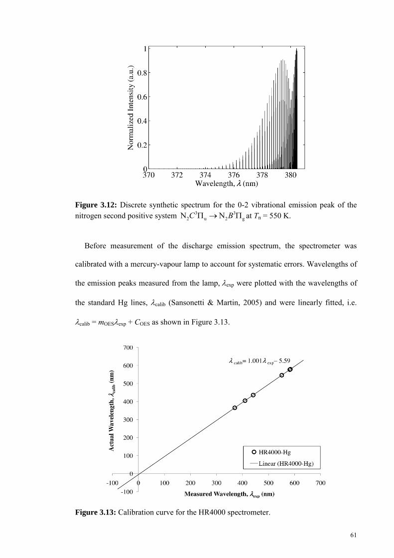
61

Figure 3.12: Discrete synthetic spectrum for the 0-2 vibrational emission peak of the nitrogen second positive system

3 32 u 2 gN NC B at Tn = 550 K.

Before measurement of the discharge emission spectrum, the spectrometer was

calibrated with a mercury-vapour lamp to account for systematic errors. Wavelengths of

the emission peaks measured from the lamp,exp were plotted with the wavelengths of

the standard Hg lines, calib (Sansonetti & Martin, 2005) and were linearly fitted, i.e.

calib = mOESexp + COES as shown in Figure 3.13.

Figure 3.13: Calibration curve for the HR4000 spectrometer.

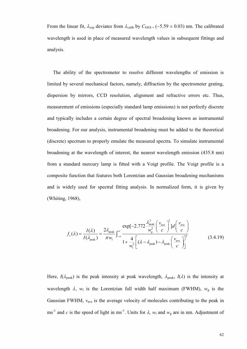
62

From the linear fit, exp deviates from calib by COES = (5.59 ± 0.03) nm. The calibrated

wavelength is used in place of measured wavelength values in subsequent fittings and

analysis.

The ability of the spectrometer to resolve different wavelengths of emission is

limited by several mechanical factors, namely, diffraction by the spectrometer grating,

dispersion by mirrors, CCD resolution, alignment and refractive errors etc. Thus,

measurement of emissions (especially standard lamp emissions) is not perfectly discrete

and typically includes a certain degree of spectral broadening known as instrumental

broadening. For our analysis, instrumental broadening must be added to the theoretical

(discrete) spectrum to properly emulate the measured spectra. To simulate instrumental

broadening at the wavelength of interest, the nearest wavelength emission (435.8 nm)

from a standard mercury lamp is fitted with a Voigt profile. The Voigt profile is a

composite function that features both Lorentzian and Gaussian broadening mechanisms

and is widely used for spectral fitting analysis. In normalized form, it is given by

(Whiting, 1968),

22peak ave ave

2peak g

v 2peak l ave

peak peak2l

exp[ 2.772 ]2( )( )

( ) 41 ( )

v vdw c cIf

I w vw c

(3.4.19)

Here, I(peak) is the peak intensity at peak wavelength, peak, I() is the intensity at

wavelength , wl is the Lorentzian full width half maximum (FWHM), wg is the

Gaussian FWHM, vave is the average velocity of molecules contributing to the peak in

ms-1 and c is the speed of light in ms-1. Units for wl and wg are in nm. Adjustment of

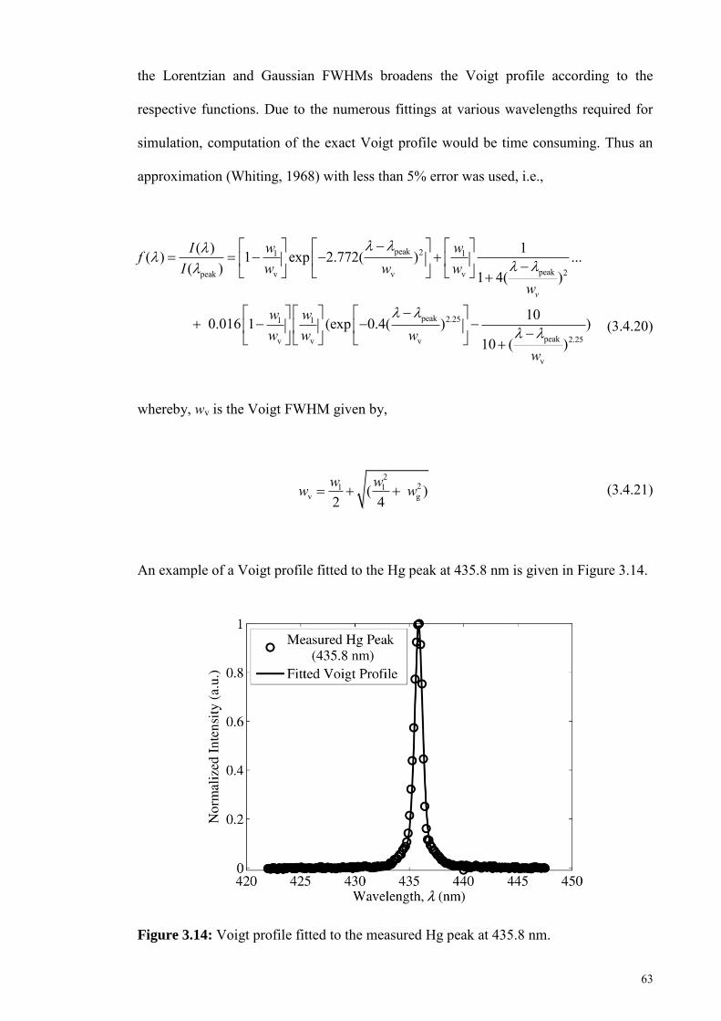
63

the Lorentzian and Gaussian FWHMs broadens the Voigt profile according to the

respective functions. Due to the numerous fittings at various wavelengths required for

simulation, computation of the exact Voigt profile would be time consuming. Thus an

approximation (Whiting, 1968) with less than 5% error was used, i.e.,

peak 2l l

peak 2peak v v v

peak 2.25l l

peak 2.25v v v

v

( ) 1( ) 1 exp 2.772( ) ...( ) 1 4( )

10 0.016 1 (exp 0.4( ) )10 ( )

v

w wIfI w w w

w

w ww w w

w

(3.4.20)

whereby, wv is the Voigt FWHM given by,

22l l

v g( )2 4w ww w (3.4.21)

An example of a Voigt profile fitted to the Hg peak at 435.8 nm is given in Figure 3.14.

Figure 3.14: Voigt profile fitted to the measured Hg peak at 435.8 nm.

64

From the fitting of measured data, wl, wg and wv were found to be 0.5 nm, 0.6 nm and

0.9 nm, respectively. These values were used to simulate instrumental broadening for all

the discrete rotational emissions of the synthetic spectra. To incorporate the broadening,

the method of convolution was used, i.e.,

conv · I I f d

(3.4.22)

Here, Iconv () is the convoluted intensity at wavelength , I (') is the intensity at the

integration wavelength'and f (') is the Voigt profile with peak wavelength at

displacement '. The result of convolution on the synthetic spectra is demonstrated in

Figure 3.15.

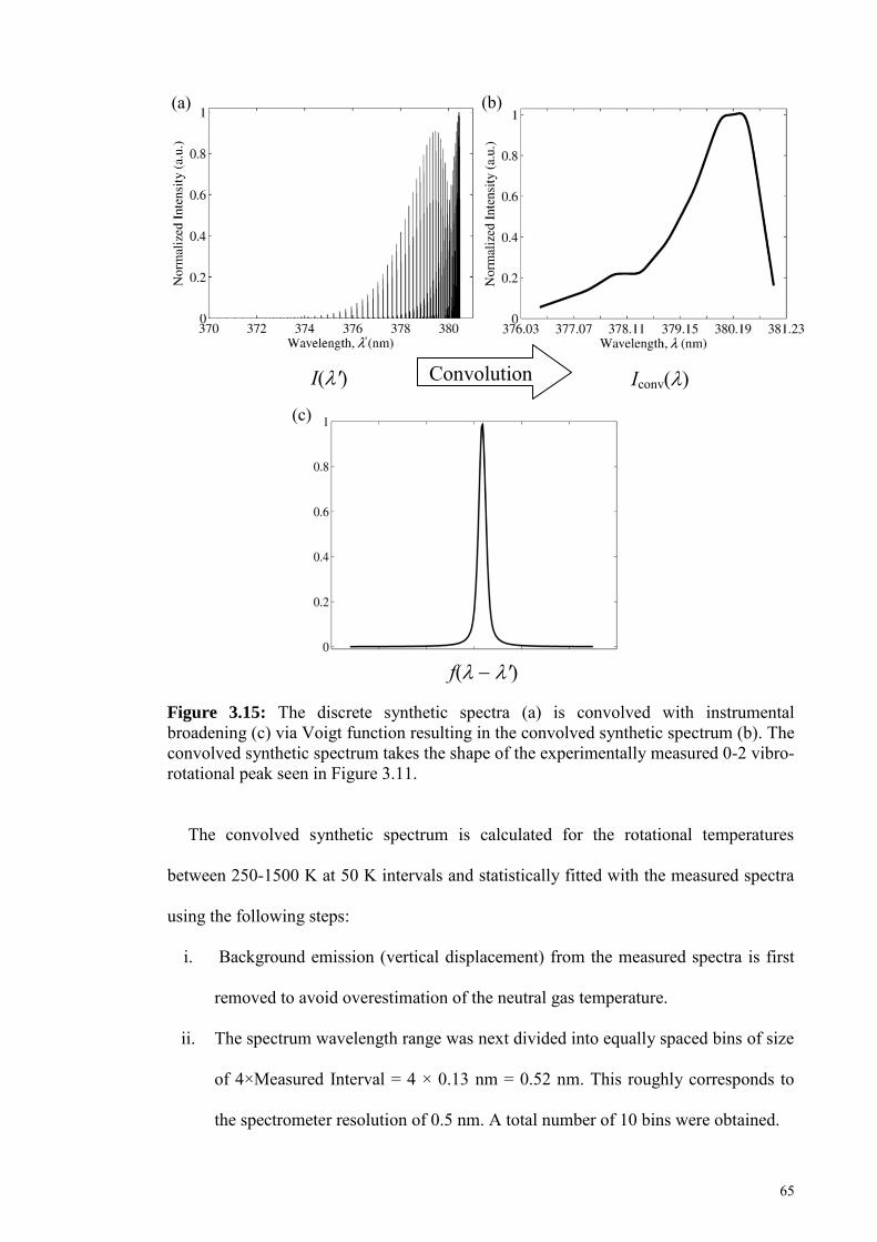
65

Figure 3.15: The discrete synthetic spectra (a) is convolved with instrumental broadening (c) via Voigt function resulting in the convolved synthetic spectrum (b). The convolved synthetic spectrum takes the shape of the experimentally measured 0-2 vibro-rotational peak seen in Figure 3.11.

The convolved synthetic spectrum is calculated for the rotational temperatures

between 250-1500 K at 50 K intervals and statistically fitted with the measured spectra

using the following steps:

i. Background emission (vertical displacement) from the measured spectra is first

removed to avoid overestimation of the neutral gas temperature.

ii. The spectrum wavelength range was next divided into equally spaced bins of size

of 4×Measured Interval = 4 × 0.13 nm = 0.52 nm. This roughly corresponds to

the spectrometer resolution of 0.5 nm. A total number of 10 bins were obtained.

Convolution I(') Iconv()

f(')

(a) (b)

(c)

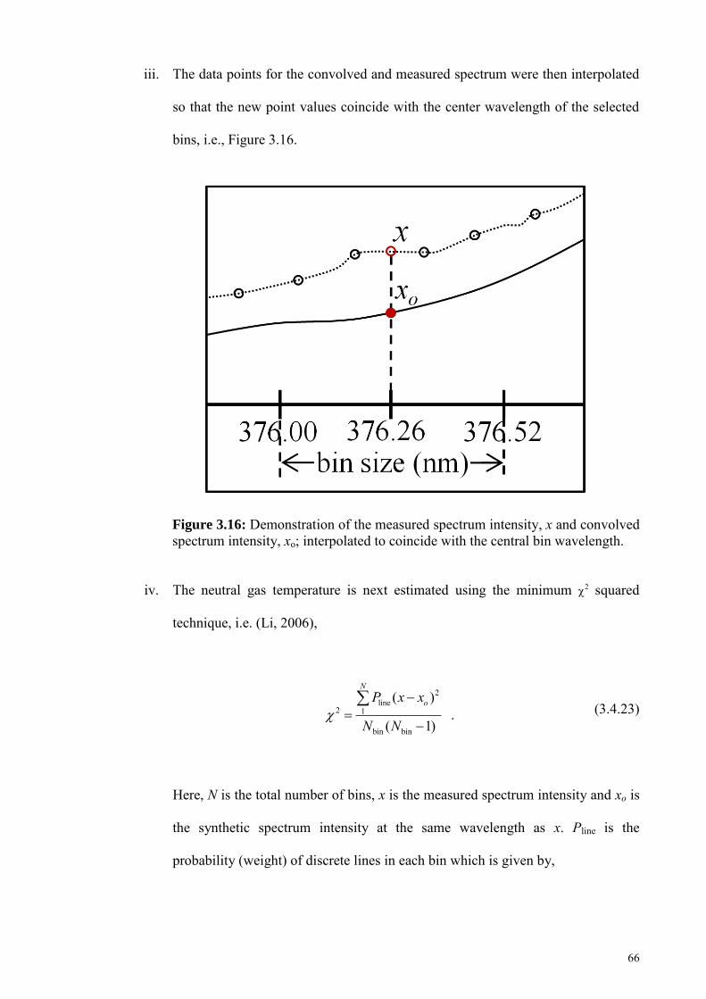
66

iii. The data points for the convolved and measured spectrum were then interpolated

so that the new point values coincide with the center wavelength of the selected

bins, i.e., Figure 3.16.

Figure 3.16: Demonstration of the measured spectrum intensity, x and convolved spectrum intensity, xo; interpolated to coincide with the central bin wavelength.

iv. The neutral gas temperature is next estimated using the minimum 2 squared

technique, i.e. (Li, 2006),

2line

2 1

bin bin

( ) .

( 1)

N

oP x x

N N

(3.4.23)

Here, N is the total number of bins, x is the measured spectrum intensity and xo is

the synthetic spectrum intensity at the same wavelength as x. Pline is the

probability (weight) of discrete lines in each bin which is given by,

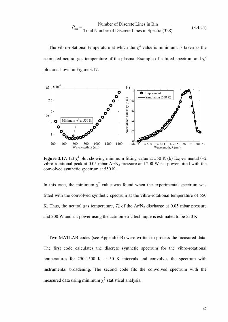
67

line

Number of Discrete Lines in BinTotal Number of Discrete Lines in Spectra (328)

P (3.4.24)

The vibro-rotational temperature at which the 2 value is minimum, is taken as the

estimated neutral gas temperature of the plasma. Example of a fitted spectrum and 2

plot are shown in Figure 3.17.

Figure 3.17: (a) χ2 plot showing minimum fitting value at 550 K (b) Experimental 0-2 vibro-rotational peak at 0.05 mbar Ar/N2 pressure and 200 W r.f. power fitted with the convolved synthetic spectrum at 550 K.

In this case, the minimum χ2 value was found when the experimental spectrum was

fitted with the convolved synthetic spectrum at the vibro-rotational temperature of 550

K. Thus, the neutral gas temperature, Tn of the Ar/N2 discharge at 0.05 mbar pressure

and 200 W and r.f. power using the actinometric technique is estimated to be 550 K.

Two MATLAB codes (see Appendix B) were written to process the measured data.

The first code calculates the discrete synthetic spectrum for the vibro-rotational

temperatures for 250-1500 K at 50 K intervals and convolves the spectrum with

instrumental broadening. The second code fits the convolved spectrum with the

measured data using minimum statistical analysis.

a) b)

68

CHAPTER 4: RESULTS AND DISCUSSION - EXPERIMENT

4.0. Measurement of Discharge Electrical Characteristics

Measurement of discharge electrical characteristics is divided to two parts. The first

part shows the measured radial distributions of electron density and electron

temperature at different pressures and axial distances above the dielectric plate. These

measurements are fitted into 2D Gaussian based distributions and subsequently used in

predictive electromagnetic simulation (Chapter 6, Section 6.0.1). The second part shows

the measured electron probability distribution function (EEPF) which is parametrically

fitted with Maxwellian and Druyvestyen distributions to provide a guided assumption of

the distribution to be used for simulation.

4.0.1. Electron Density, ne and Electron Temperature, Te

Figures 4.1, 4.2 and 4.3 show the radial distributions of the (i) electron densities, ne

and (ii) electron temperatures, Te for three argon pressures (0.03 mbar, 0.07 mbar and

0.2 mbar) measured at 0.032 m, 0.060 m and 0.114 m axial distances above the

dielectric plate, respectively. R.f. power was set at 180 W. The label suffixes 'a' and 'b'

(e.g. Figure 4.1a) denote the Maxwellian and EEDF calculation methods, respectively.

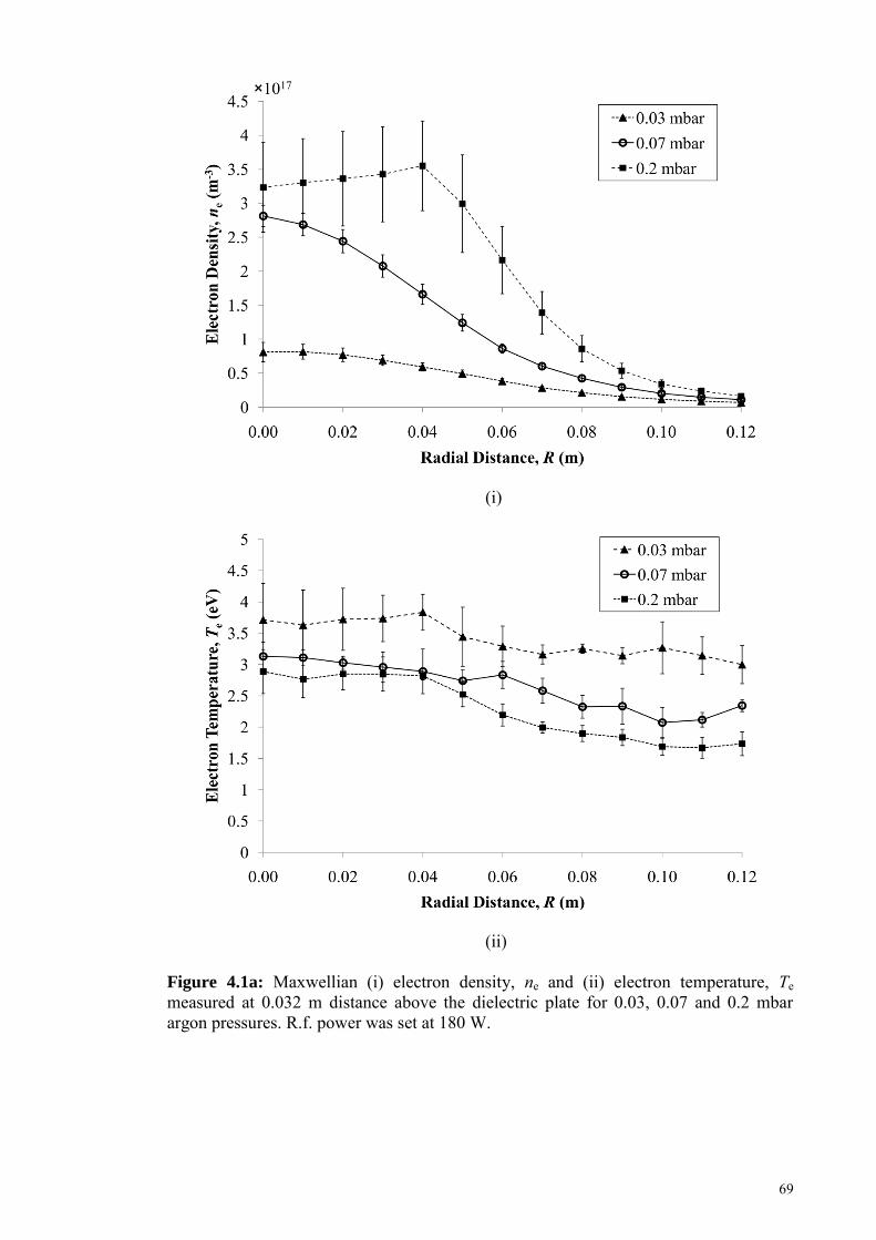
69

(i)

(ii)

Figure 4.1a: Maxwellian (i) electron density, ne and (ii) electron temperature, Te measured at 0.032 m distance above the dielectric plate for 0.03, 0.07 and 0.2 mbar argon pressures. R.f. power was set at 180 W.

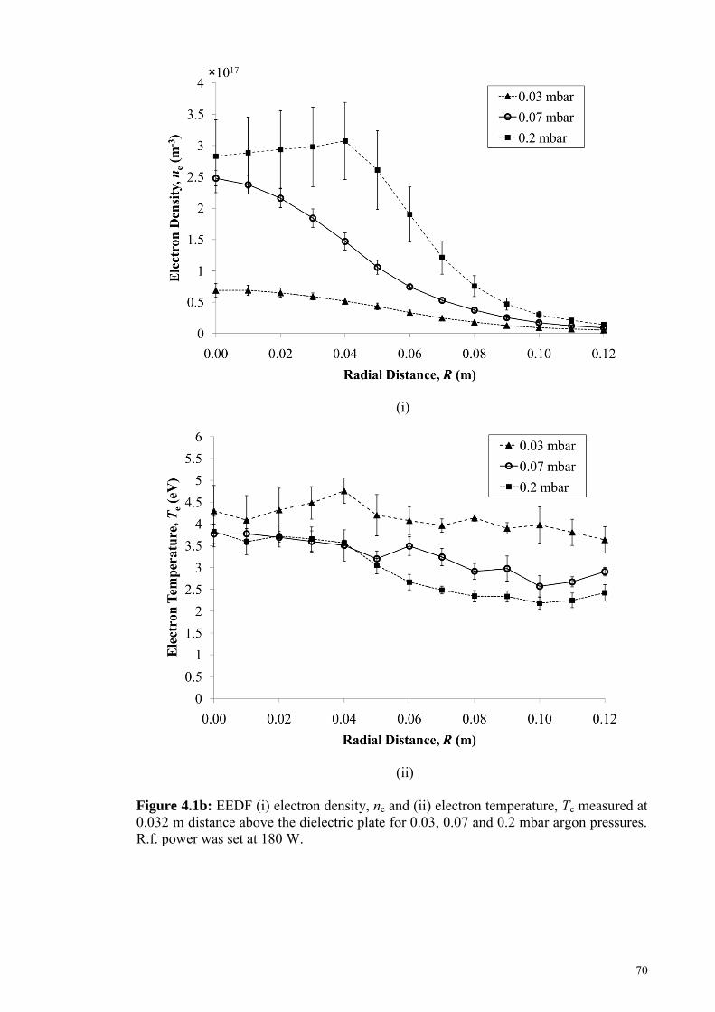
70

(i)

(ii)

Figure 4.1b: EEDF (i) electron density, ne and (ii) electron temperature, Te measured at 0.032 m distance above the dielectric plate for 0.03, 0.07 and 0.2 mbar argon pressures. R.f. power was set at 180 W.

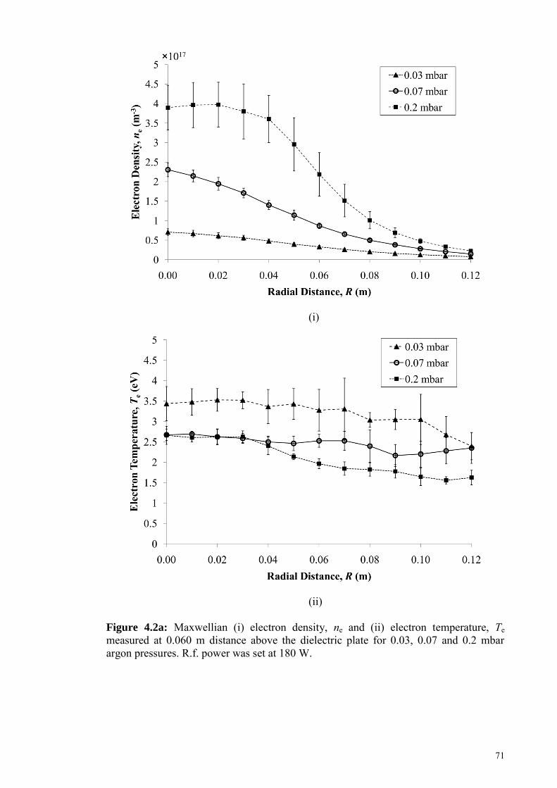
71

(i)

(ii)

Figure 4.2a: Maxwellian (i) electron density, ne and (ii) electron temperature, Te measured at 0.060 m distance above the dielectric plate for 0.03, 0.07 and 0.2 mbar argon pressures. R.f. power was set at 180 W.

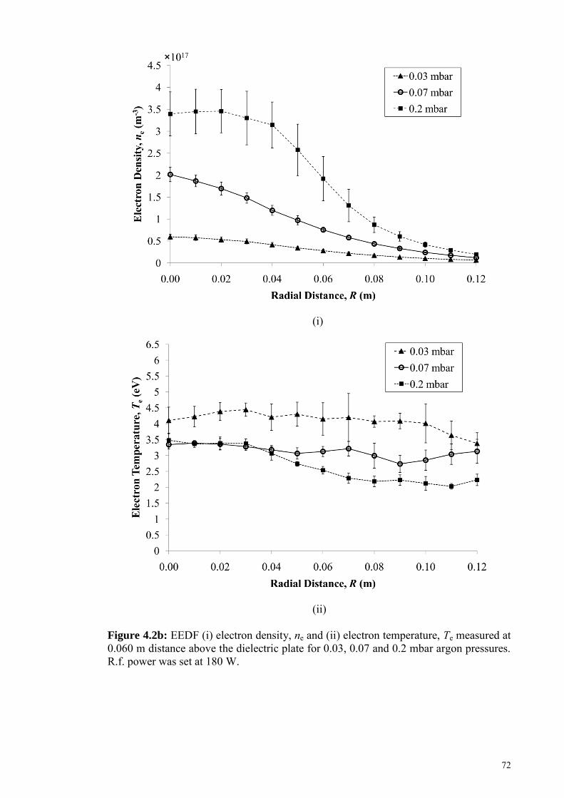
72

(i)

(ii)

Figure 4.2b: EEDF (i) electron density, ne and (ii) electron temperature, Te measured at 0.060 m distance above the dielectric plate for 0.03, 0.07 and 0.2 mbar argon pressures. R.f. power was set at 180 W.

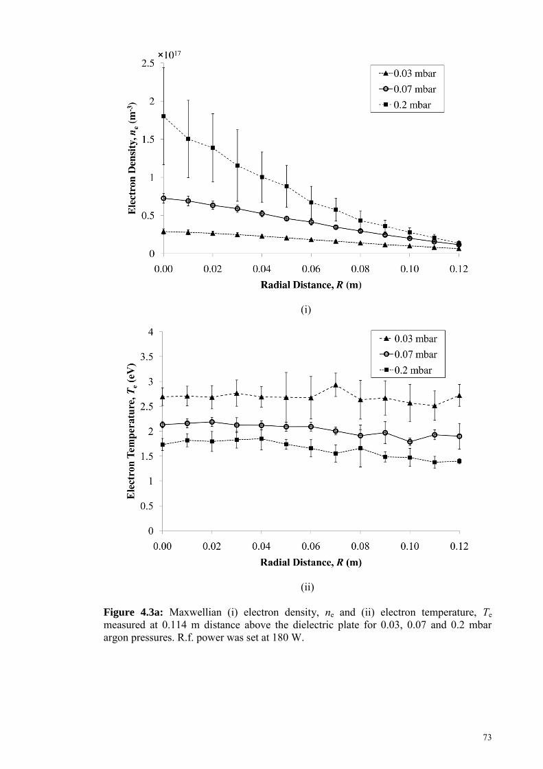
73

(i)

(ii)

Figure 4.3a: Maxwellian (i) electron density, ne and (ii) electron temperature, Te measured at 0.114 m distance above the dielectric plate for 0.03, 0.07 and 0.2 mbar argon pressures. R.f. power was set at 180 W.

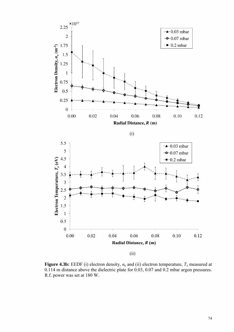
74

(i)

(ii)

Figure 4.3b: EEDF (i) electron density, ne and (ii) electron temperature, Te measured at 0.114 m distance above the dielectric plate for 0.03, 0.07 and 0.2 mbar argon pressures. R.f. power was set at 180 W.

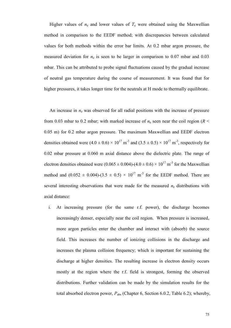
75

Higher values of ne and lower values of Te were obtained using the Maxwellian

method in comparison to the EEDF method; with discrepancies between calculated

values for both methods within the error bar limits. At 0.2 mbar argon pressure, the

measured deviation for ne is seen to be larger in comparison to 0.07 mbar and 0.03

mbar. This can be attributed to probe signal fluctuations caused by the gradual increase

of neutral gas temperature during the course of measurement. It was found that for

higher pressures, it takes longer time for the neutrals at H mode to thermally equilibrate.

An increase in ne was observed for all radial positions with the increase of pressure

from 0.03 mbar to 0.2 mbar; with marked increase of ne seen near the coil region (R <

0.05 m) for 0.2 mbar argon pressure. The maximum Maxwellian and EEDF electron

densities obtained were (4.0 ± 0.6) × 1017 m-3 and (3.5 ± 0.5) × 1017 m-3, respectively for

0.02 mbar pressure at 0.060 m axial distance above the dielectric plate. The range of

electron densities obtained were (0.065 ± 0.004)-(4.0 ± 0.6) × 1017 m-3 for the Maxwellian

method and (0.052 ± 0.004)-(3.5 ± 0.5) × 1017 m-3 for the EEDF method. There are

several interesting observations that were made for the measured ne distributions with

axial distance:

i. At increasing pressure (for the same r.f. power), the discharge becomes

increasingly denser, especially near the coil region. When pressure is increased,

more argon particles enter the chamber and interact with (absorb) the source

field. This increases the number of ionizing collisions in the discharge and

increases the plasma collision frequency; which is important for sustaining the

discharge at higher densities. The resulting increase in electron density occurs

mostly at the region where the r.f. field is strongest, forming the observed

distributions. Further validation can be made by the simulation results for the

total absorbed electron power, Pabs (Chapter 6, Section 6.0.2, Table 6.2); whereby,

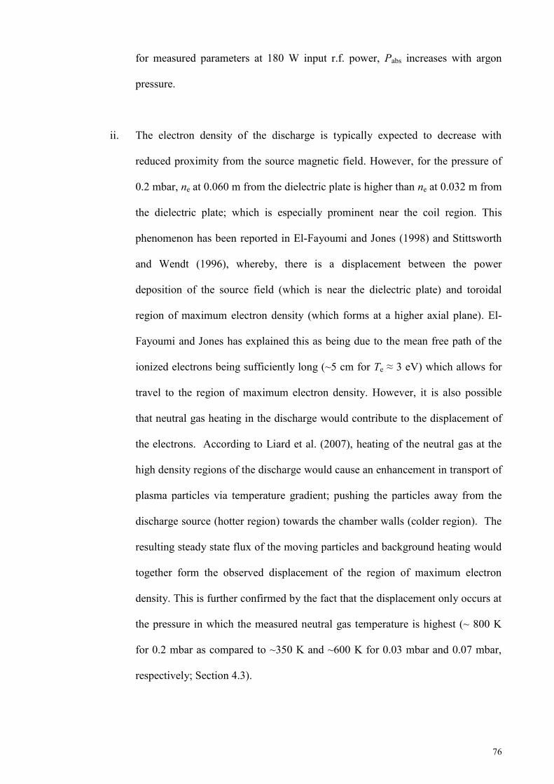
76

for measured parameters at 180 W input r.f. power, Pabs increases with argon

pressure.

ii. The electron density of the discharge is typically expected to decrease with

reduced proximity from the source magnetic field. However, for the pressure of

0.2 mbar, ne at 0.060 m from the dielectric plate is higher than ne at 0.032 m from

the dielectric plate; which is especially prominent near the coil region. This

phenomenon has been reported in El-Fayoumi and Jones (1998) and Stittsworth

and Wendt (1996), whereby, there is a displacement between the power

deposition of the source field (which is near the dielectric plate) and toroidal

region of maximum electron density (which forms at a higher axial plane). El-

Fayoumi and Jones has explained this as being due to the mean free path of the

ionized electrons being sufficiently long (~5 cm for Te ≈ 3 eV) which allows for

travel to the region of maximum electron density. However, it is also possible

that neutral gas heating in the discharge would contribute to the displacement of

the electrons. According to Liard et al. (2007), heating of the neutral gas at the

high density regions of the discharge would cause an enhancement in transport of

plasma particles via temperature gradient; pushing the particles away from the

discharge source (hotter region) towards the chamber walls (colder region). The

resulting steady state flux of the moving particles and background heating would

together form the observed displacement of the region of maximum electron

density. This is further confirmed by the fact that the displacement only occurs at

the pressure in which the measured neutral gas temperature is highest (~ 800 K

for 0.2 mbar as compared to ~350 K and ~600 K for 0.03 mbar and 0.07 mbar,

respectively; Section 4.3).

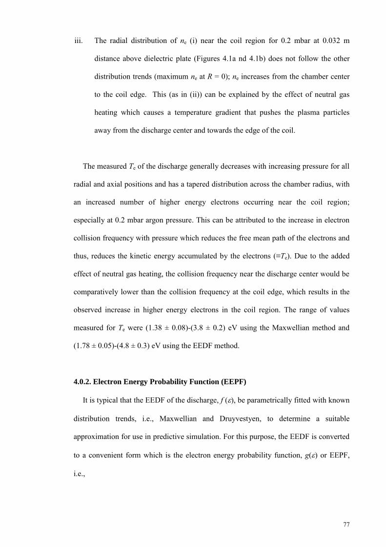
77

iii. The radial distribution of ne (i) near the coil region for 0.2 mbar at 0.032 m

distance above dielectric plate (Figures 4.1a nd 4.1b) does not follow the other

distribution trends (maximum ne at R = 0); ne increases from the chamber center

to the coil edge. This (as in (ii)) can be explained by the effect of neutral gas

heating which causes a temperature gradient that pushes the plasma particles

away from the discharge center and towards the edge of the coil.

The measured Te of the discharge generally decreases with increasing pressure for all

radial and axial positions and has a tapered distribution across the chamber radius, with

an increased number of higher energy electrons occurring near the coil region;

especially at 0.2 mbar argon pressure. This can be attributed to the increase in electron

collision frequency with pressure which reduces the free mean path of the electrons and

thus, reduces the kinetic energy accumulated by the electrons (≡Te). Due to the added

effect of neutral gas heating, the collision frequency near the discharge center would be

comparatively lower than the collision frequency at the coil edge, which results in the

observed increase in higher energy electrons in the coil region. The range of values

measured for Te were (1.38 ± 0.08)-(3.8 ± 0.2) eV using the Maxwellian method and

(1.78 ± 0.05)-(4.8 ± 0.3) eV using the EEDF method.

4.0.2. Electron Energy Probability Function (EEPF)

It is typical that the EEDF of the discharge, f (), be parametrically fitted with known

distribution trends, i.e., Maxwellian and Druyvestyen, to determine a suitable

approximation for use in predictive simulation. For this purpose, the EEDF is converted

to a convenient form which is the electron energy probability function, g() or EEPF,

i.e.,

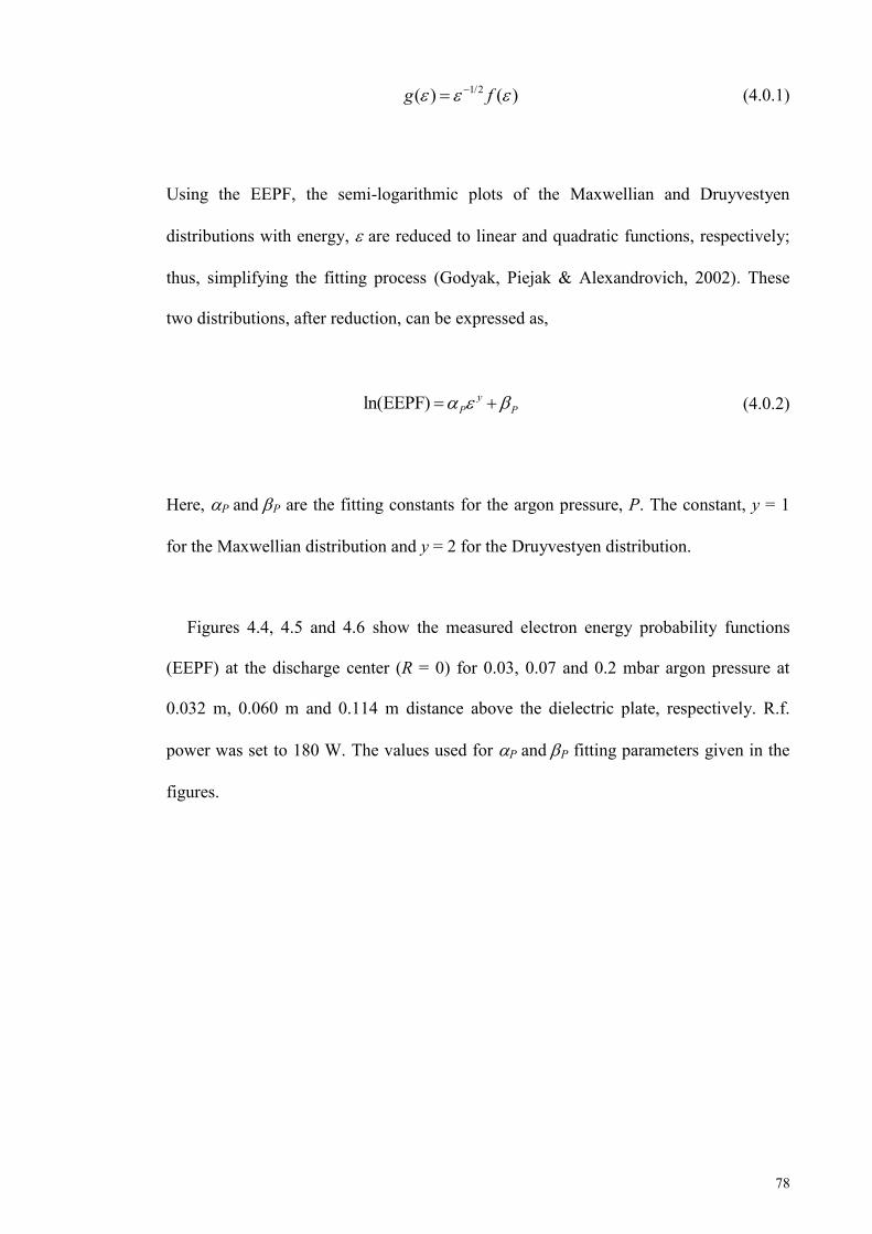
78

1/2( ) ( )g f (4.0.1)

Using the EEPF, the semi-logarithmic plots of the Maxwellian and Druyvestyen

distributions with energy, are reduced to linear and quadratic functions, respectively;

thus, simplifying the fitting process (Godyak, Piejak & Alexandrovich, 2002). These

two distributions, after reduction, can be expressed as,

ln(EEPF) yP P (4.0.2)

Here, PandP are the fitting constants for the argon pressure, P. The constant, y = 1

for the Maxwellian distribution and y = 2 for the Druyvestyen distribution.

Figures 4.4, 4.5 and 4.6 show the measured electron energy probability functions

(EEPF) at the discharge center (R = 0) for 0.03, 0.07 and 0.2 mbar argon pressure at

0.032 m, 0.060 m and 0.114 m distance above the dielectric plate, respectively. R.f.

power was set to 180 W. The values used for PandP fitting parameters given in the

figures.

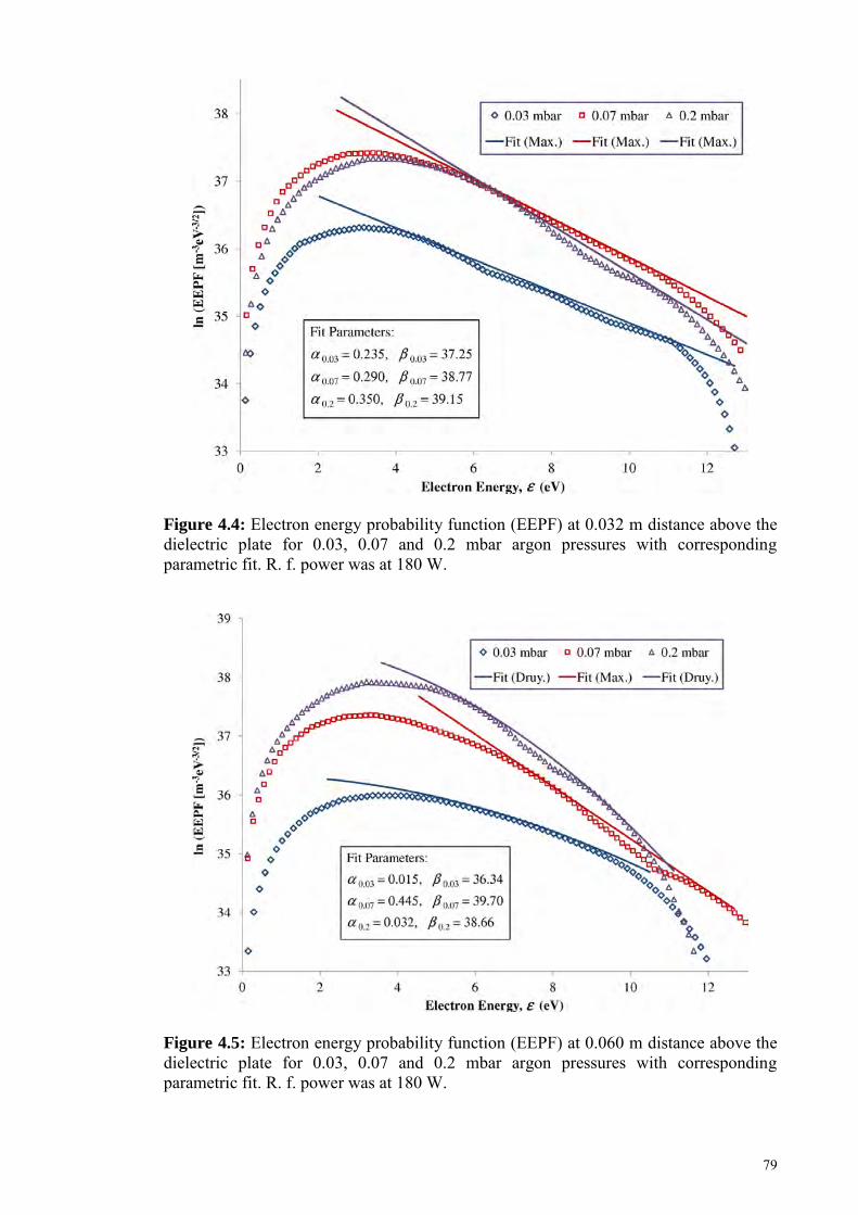
79

Figure 4.4: Electron energy probability function (EEPF) at 0.032 m distance above the dielectric plate for 0.03, 0.07 and 0.2 mbar argon pressures with corresponding parametric fit. R. f. power was at 180 W.

Figure 4.5: Electron energy probability function (EEPF) at 0.060 m distance above the dielectric plate for 0.03, 0.07 and 0.2 mbar argon pressures with corresponding parametric fit. R. f. power was at 180 W.

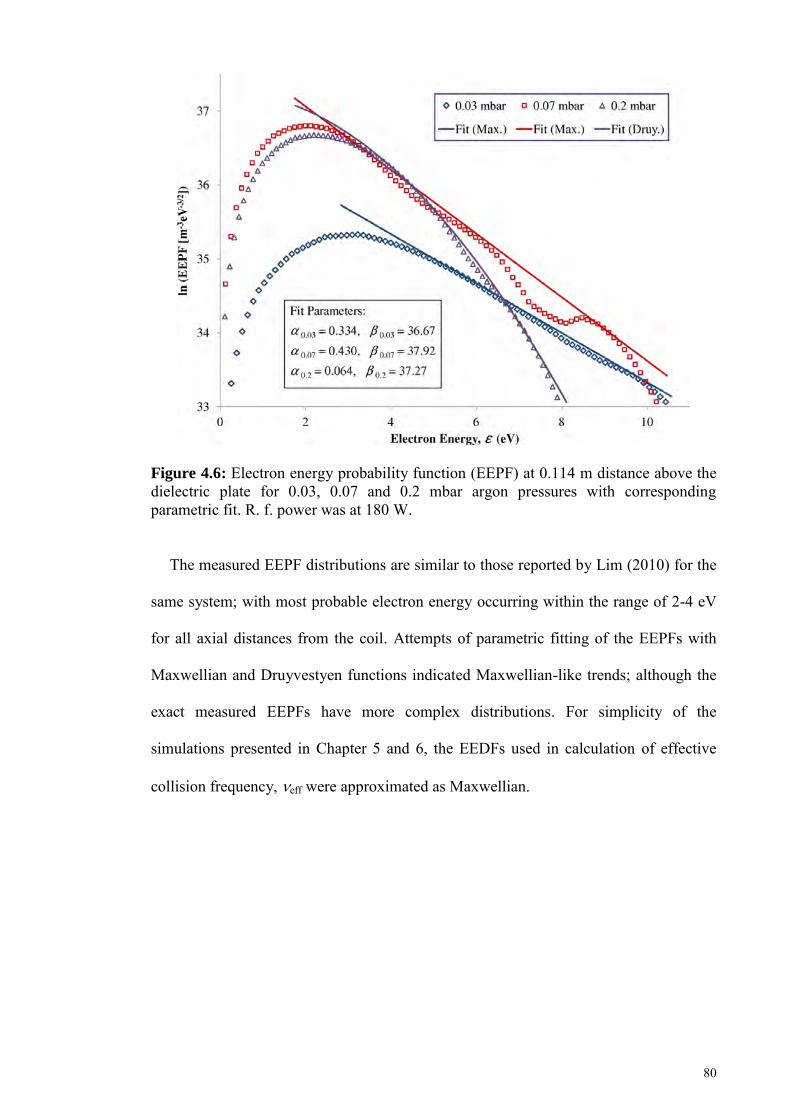
80

Figure 4.6: Electron energy probability function (EEPF) at 0.114 m distance above the dielectric plate for 0.03, 0.07 and 0.2 mbar argon pressures with corresponding parametric fit. R. f. power was at 180 W.

The measured EEPF distributions are similar to those reported by Lim (2010) for the

same system; with most probable electron energy occurring within the range of 2-4 eV

for all axial distances from the coil. Attempts of parametric fitting of the EEPFs with

Maxwellian and Druyvestyen functions indicated Maxwellian-like trends; although the

exact measured EEPFs have more complex distributions. For simplicity of the

simulations presented in Chapter 5 and 6, the EEDFs used in calculation of effective

collision frequency, eff were approximated as Maxwellian.

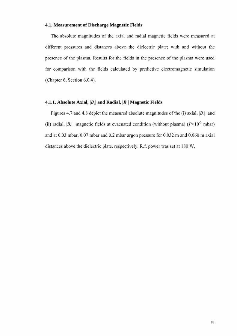
81

4.1. Measurement of Discharge Magnetic Fields

The absolute magnitudes of the axial and radial magnetic fields were measured at

different pressures and distances above the dielectric plate; with and without the

presence of the plasma. Results for the fields in the presence of the plasma were used

for comparison with the fields calculated by predictive electromagnetic simulation

(Chapter 6, Section 6.0.4).

4.1.1. Absolute Axial, |Bz| and Radial, |Br| Magnetic Fields

Figures 4.7 and 4.8 depict the measured absolute magnitudes of the (i) axial, |Bz| and

(ii) radial, |Br| magnetic fields at evacuated condition (without plasma) (P<10-3 mbar)

and at 0.03 mbar, 0.07 mbar and 0.2 mbar argon pressure for 0.032 m and 0.060 m axial

distances above the dielectric plate, respectively. R.f. power was set at 180 W.

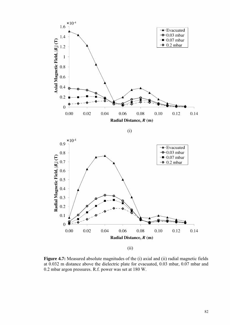
82

(i)

(ii)

Figure 4.7: Measured absolute magnitudes of the (i) axial and (ii) radial magnetic fields at 0.032 m distance above the dielectric plate for evacuated, 0.03 mbar, 0.07 mbar and 0.2 mbar argon pressures. R.f. power was set at 180 W.

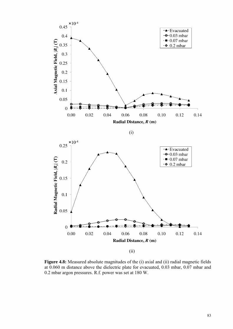
83

(i)

(ii)

Figure 4.8: Measured absolute magnitudes of the (i) axial and (ii) radial magnetic fields at 0.060 m distance above the dielectric plate for evacuated, 0.03 mbar, 0.07 mbar and 0.2 mbar argon pressures. R.f. power was set at 180 W.

84

When the chamber is evacuated (without plasma), the measured axial and radial

magnetic fields gave the highest magnitudes with (1.507 ± 0.005) × 10-4 T and (7.67 ±

0.01) × 10 -5 T, respectively for 0.032 m and (3.90 ± 0.02) × 10-5 T and (2.30 ± 0.03) ×

10-5 T, respectively for 0.060 m. The peak coil current, Ip obtained when measuring the

magnetic fields were (19.2 ± 0.2) A at evacuated condition, (14.4 ± 0.2) A at 0.03 mbar,

(14.2 ± 0.2) A at 0.07 mbar and (13.4 ± 0.2) at 0.2 mbar.

Increased suppression of the magnetic field magnitudes was seen as pressure was

increased for both the axial and radial magnetic fields at both distances above the

dielectric plate; indicating increased utilization of the magnetic fields by the plasma.

With increase of pressure, it is also noted that a trough is formed in both the axial and

radial magnetic field magnitudes within the coil region (R < 0.05 m), whereby the

magnetic fields near the center of the chamber is more highly utilized. This is

consistent with the trends seen in the electron density in Figures 4.1 and 4.2 at which the

discharge becomes more confined to the coil region and less diffused as pressure is

increased. Beyond the coil region (R > 0.05 m), the field is to be out of phase and is

negative (when plotted as absolute values, the field is positive and inverted). This is

mainly due to the geometry of the chamber in which the coil, chamber and dielectric

diameters are different.

4.2. Measurement of Peak Coil Transition and Maintenance Currents

The H mode peak coil transition and maintenance currents were measured for a range

of argon pressures. These values were compared with predictive simulation of the

currents using the power deposition model (Chapter 6, Section 6.1).

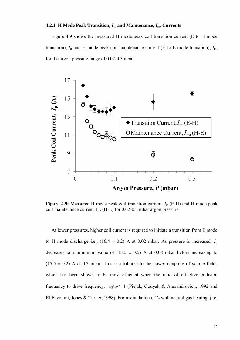
85

4.2.1. H Mode Peak Transition, Itr and Maintenance, Imt Currents

Figure 4.9 shows the measured H mode peak coil transition current (E to H mode

transition), Itr and H mode peak coil maintenance current (H to E mode transition), Imt

for the argon pressure range of 0.02-0.3 mbar.

Figure 4.9: Measured H mode peak coil transition current, Itr (E-H) and H mode peak coil maintenance current, Imt (H-E) for 0.02-0.2 mbar argon pressure.

At lower pressures, higher coil current is required to initiate a transition from E mode

to H mode discharge i.e., (16.4 ± 0.2) A at 0.02 mbar. As pressure is increased, Itr

decreases to a minimum value of (13.5 ± 0.5) A at 0.08 mbar before increasing to

(15.5 ± 0.2) A at 0.3 mbar. This is attributed to the power coupling of source fields

which has been shown to be most efficient when the ratio of effective collision

frequency to drive frequency, eff≈ 1 (Piejak, Godyak & Alexandrovich, 1992 and

El-Fayoumi, Jones & Turner, 1998). From simulation of Itr with neutral gas heating (i.e.,

86

Section 6.1.2.), eff≈ 1 is found near the measured argon pressure range of 0.07-0.08

mbar; at which least current is required to initiate a transition to H mode.

In the case of Imt, higher values are also required to maintain the discharge in H mode

operation at low pressures, i.e., (14.3 ± 0.2) A at 0.02 mbar. As pressure is increased, Imt

decreases to (8.3 ± 0.1) A at 0.3 mbar. The increasing deviation between Itr and Imt with

increasing pressure indicates the more prominent effect of hysteresis in the working

path of the system. The effect of hysteresis is more thoroughly discussed in Chapter 6.

Several factors can be attributed to the lower Imt requirement for the discharge at higher

pressures:

i. At higher pressures, the electron density of the H mode discharge is higher.

Multi-step ionization (i.e., ionization of the neutrals through intermediate

excitation states) becomes the primary process of conversion of absorbed excited

state energy over radiative de-excitation processes (Turner and Lieberman, 1999).

Thus, more energy from the excitation collisions that occur in the discharge

contributes toward the ionization of particles, allowing for maintenance of the H

mode discharge at lower currents.

ii. At higher pressures, there are also more plasma particles that are present in the

chamber. The increase in collision frequency of these particles would also result

in more ionizing collisions, which allows for maintenance of the H mode

discharge at lower currents.

iii. The neutral gas temperature of the discharge is also seen to increase (in reference

to Section 4.3) at higher pressure. This may result in the neutral particles being

more readily ionized due to more of the background particles having higher

87

kinetic energies. This may have some contribution in enabling the sustenance of

the H mode discharge at lower currents for higher pressures.

4.3. Measurement of Discharge Neutral Gas Temperature via AOES

Using the AOES technique, the neutral gas temperature of the discharge was

measured at different pressures and distances above the dielectric plate for increasing

and decreasing input r.f. powers. Results from measurement were taken as reference for

the predictive simulations found in Chapter 6.

4.3.1. Measured Neutral Gas Temperature, Tn

Figure 4.10 and 4.11 shows the measured neutral gas temperatures, Tn at 0.03, 0.05,

0.07, 0.1 and 0.2 mbar Ar/N2 pressure for (i) increasing and (ii) decreasing r.f. power at

0.032 m and 0.060 m axial distance above the dielectric plate, respectively.

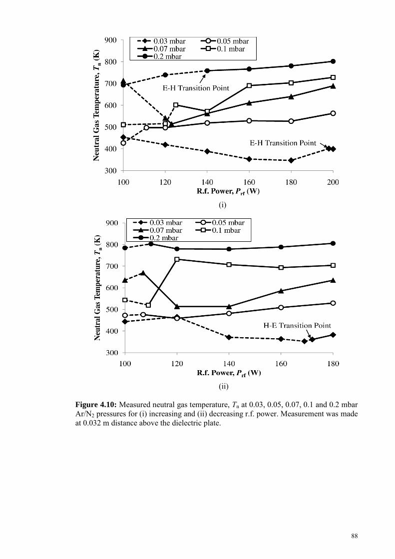
88

(i)

(ii)

Figure 4.10: Measured neutral gas temperature, Tn at 0.03, 0.05, 0.07, 0.1 and 0.2 mbar Ar/N2 pressures for (i) increasing and (ii) decreasing r.f. power. Measurement was made at 0.032 m distance above the dielectric plate.

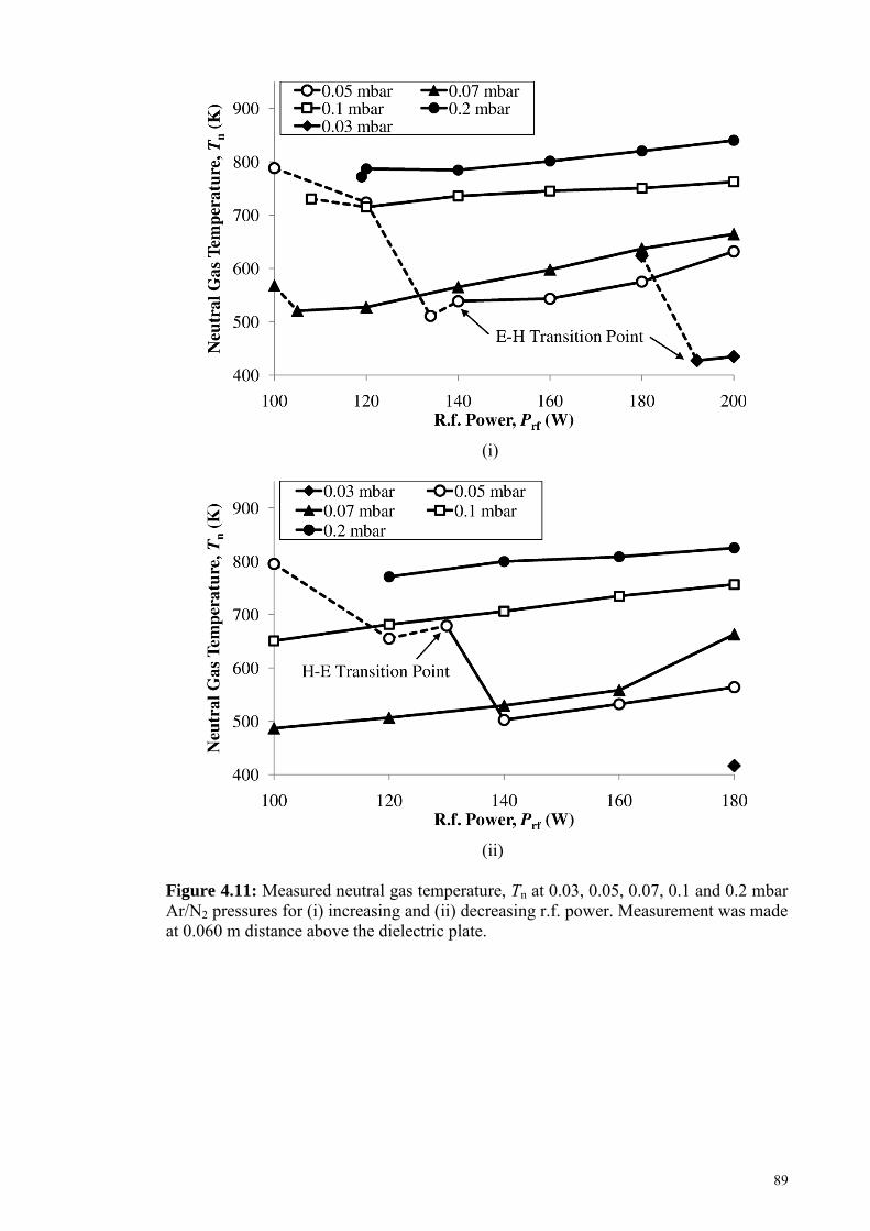
89

(i)

(ii)

Figure 4.11: Measured neutral gas temperature, Tn at 0.03, 0.05, 0.07, 0.1 and 0.2 mbar Ar/N2 pressures for (i) increasing and (ii) decreasing r.f. power. Measurement was made at 0.060 m distance above the dielectric plate.

90

The dashed lines on the plots represent the discharge at E mode state, whereas, the

solid lines represent the discharge in H mode state. The mode transition point is the

point between the dashed and solid lines. Tn measured in E mode state had higher errors

on average (i.e., 10-20 % error for the discharge in E mode compared to 5-12 % error in

H mode) due to the lower definitions of the fitted peak, especially for 0.060 m distance

above the dielectric plate. At certain powers, Tn was not measured due to the reference

peak being not of resolvable intensity.

With r.f. power and distance above the dielectric plate, Tn is seen to have little

variation; within the bounds of measured error. With increase in gas pressure, however,

Tn becomes markedly increased. These observed trends are explained as follows:

i. As Ar/N2 pressure is increased at a fixed input r.f. power, more energy is coupled

into the plasma. This is demonstrated by calculations tabulated in Chapter 6,

Section 6.0.2, Table 6.2, whereby, absorbed electron power, Pabs is higher at

higher pressure, P for the same input r.f. power of 180 W. With increased power

coupled into the discharge, electron density and ion density increases. Because of

the presence of more charged and neutral particles within the same volume for

higher pressure, the collision frequency of the plasma particles increases.

Transfer of kinetic energy from charged particles to neutral particles is increased

via charge transfer collision of energetic ions with neutrals and de-excitation

collision of ions by electrons (Lieberman & Lichtenberg, 2005). This raises the

number of thermalized neutrals within the plasma, thus, increasing Tn.

ii. With collisional processes between charged and neutral particles limited by the

collision frequency which is correlated with Ar/N2 pressure (as mentioned in the

91

previous point, i.), variation of r.f. power does not significantly affect Tn; due to

the limited energy transfer from charged particles to the neutrals.

iii. The convection of thermalized neutrals from "hotter" plasma regions (i.e., nearer

to the source field, where the discharge is more intense) to colder regions (away

from the source field) would mean that the particles would also be distributed to

regions further from the source (noted in Section 4.0.1 for electron density). Thus,

at the measured axial distances of 0.032 m and 0.060 m, Tn does not show

significant variation beyond the discrepancy obtained in measurement.

For increasing r.f. power at H mode and 0.032 m plate distance, values of Tn ranged

from (350 ± 30) K at 0.03 mbar to (800 ± 20) K at 0.2 mbar. For decreasing r.f. power

at H mode and 0.032 m plate distance, values of Tn were from (380 ± 10) K at 0.03

mbar to (810 ± 20) K at 0.2 mbar. In the case of increasing r.f. power at H mode and

0.060 m plate distance, values for Tn ranged from (430 ± 20) K at 0.03 mbar to

(840 ± 30) K at 0.2 mbar. For decreasing r.f. power at H mode and 0.060 m plate

distance, values for Tn were from (420 ± 20) K at 0.03 mbar to (830 ± 30) K at 0.2

mbar. These values of Tn will be used as a reference range for the simulations shown in

Chapter 6.

92

CHAPTER 5: SIMULATION

5.0. Electromagnetic Field Model

Simulation of the E mode and H mode electromagnetic fields used in this work

(Sections 5.1, 5.2, 5.3 and 5.4) is based on the field theory derived by El-Fayoumi et al.

(El-Fayoumi, 1996; El-Fayoumi & Jones, 1998; El-Fayoumi, Jones & Turner, 1998). To

obtain a more accurate representation of the laboratory ICP reactor fields, certain

aspects of the original model were improved. These include:

i. Modifications of the model field grid to more closely resemble the actual

dimensions of the laboratory reactor.

ii. Independent adjustment of radius of the planar coil source, quartz dielectric plate

and chamber.

iii. Extended calculation of the collision frequency parameter; accounting for the

effects of important collisional processes.

iv. Spatially resolved plasma parameters such as electron density, electron

temperature and neutral gas temperature; which interact with the fields.

The E mode and H mode electromagnetic fields in the laboratory ICP reactor are

modeled in cylindrical coordinates (r, , z) with the following measured dimensions:

radius of the 6-turn planar coil, a = 0.045 m; radius of the 0.010 m thick quartz

dielectric plate, d = 0.100 m; inner radius of chamber, b = 0.145 m; full inner height of

chamber, H = 0.304 m; effective height of chamber, L = 0.218 m; height of indented

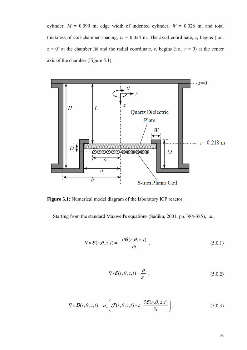
93

cylinder, M = 0.099 m; edge width of indented cylinder, W = 0.026 m; and total

thickness of coil-chamber spacing, D = 0.024 m. The axial coordinate, z, begins (i.e.,

z = 0) at the chamber lid and the radial coordinate, r, begins (i.e., r = 0) at the center

axis of the chamber (Figure 5.1).

Figure 5.1: Numerical model diagram of the laboratory ICP reactor.

Starting from the standard Maxwell's equations (Sadiku, 2001, pp. 384-385), i.e.,

( , , , )( , , , ) ,r z tr z tt

(5.0.1)

o

( , , , ) ,r z t

(5.0.2)

o o

( , , , )( , , , ) ( , , , ) ,r z tr z t r z tt

(5.0.3)

94

and

( , , , ) 0 ,r z t (5.0.4)

the following assumptions were applied:

i. The reactor is azimuthally symmetric, thus, the fields only vary in the -r and -z

directions.

ii. The plasma mainly consists of low energy electrons and the immobile ions thus,

satisfying the local Ohm’s Law equation,

e2

e

( , , , )( , , , ) ( , , , ) ,m r z tr z t r z tn e t

(5.0.5)

where, me is the electronic mass in kg, e is the electronic charge in C, ne is the

electron density in m-3 and is the electron collision frequency in s-1.

iii. For free space, the charge density term, , thus, reducing Eq. (5.0.2) to,

( , , , ) 0 .r z t (5.0.6)

iv. The steady state temporal term of the r.f. field is represented by exp(jt), where

is the r.f. angular frequency (rad/s), i.e., 2× 13.56 MHz .

Here, , and are the time varying electric field in Vm-1, magnetic field in T and

current density in Am-2, respectively. ois the free space permeability in Hm-1 and o is

95

the free space permittivity in Fm-1. With these assumptions, Eqs. (5.0.1-5.0.5) can be

subsequently simplified as,

( , ) ( , ) ,r z j r z E B (5.0.7)

( , ) 0 ,r z E (5.0.8)

o o o( , ) ( , ) ( , ) ,r z r z j r z B J E (5.0.9)

( , ) 0 ,r z B (5.0.10)

and

2o p( , ) ( , ) ,r z r z

j

J E (5.0.11)

p is the plasma frequency in s-1 and is given by,

1/22e

po e

.n em

(5.0.12)

The equations were solved both analytically and numerically for the H mode fields

with the initial field values for boundary convergence of the numerical solution being

analytically derived. Analytical E mode fields were also derived for use in the power

balance model in Section 5.4. Solutions for each of the fields are addressed separately in

the following sections.

96

5.1. Analytical H mode fields

To solve for the analytical H mode fields from Eqs. (5.0.7-5.0.12), further

assumptions and boundary conditions were applied:

a) The displacement current term in Eq. (5.0.9) is neglected (i.e., jooE(r,z) = 0). This

is due to the higher free excitation wavelength (~22 m for 13.56 MHz) as

compared to the chamber dimensions. Eq. (5.0.9) then reduces to,

o( , ) ( , ) .r z r z B J (5.1.1)

b) The planar coil is assumed to be an infinitesimally thin disc of moving uniform

charge and has a surface current density of,

p ,NI

Ka (5.1.2)

where Ip is the peak coil current in A, N is the number of turns in the coil and a is

the coil radius in m.

c) The chamber is a simple azimuthally symmetric cylinder of radius, b and

effective height, L with a coil radius of a. The coil-chamber spacing is D (Figure

5.2).

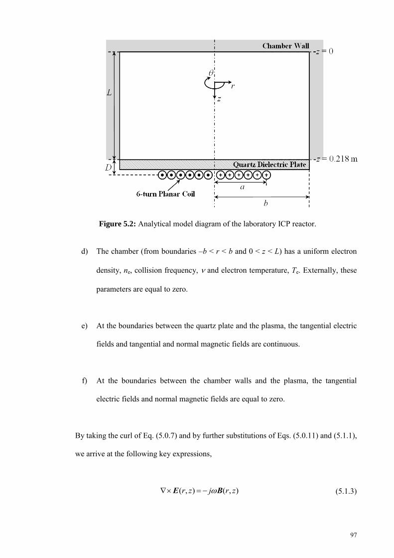
97

Figure 5.2: Analytical model diagram of the laboratory ICP reactor.

d) The chamber (from boundaries –b < r < b and 0 < z < L) has a uniform electron

density, ne, collision frequency, and electron temperature, Te. Externally, these

parameters are equal to zero.

e) At the boundaries between the quartz plate and the plasma, the tangential electric

fields and tangential and normal magnetic fields are continuous.

f) At the boundaries between the chamber walls and the plasma, the tangential

electric fields and normal magnetic fields are equal to zero.

By taking the curl of Eq. (5.0.7) and by further substitutions of Eqs. (5.0.11) and (5.1.1),

we arrive at the following key expressions,

( , ) ( , )r z j r z E B (5.1.3)

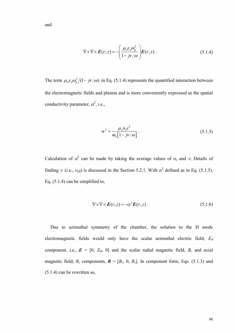
98

and

2o o p( , ) ( , ) .

1r z r z

j

E E (5.1.4)

The term 2o o p (1 )j in Eq. (5.1.4) represents the quantified interaction between

the electromagnetic fields and plasma and is more conveniently expressed as the spatial

conductivity parameter, ,i.e.,

22 o e

e

.1

n em j

(5.1.5)

Calculation of 2 can be made by taking the average values of ne and . Details of

finding i.e.,eff is discussed in the Section 5.2.1. With 2 defined as in Eq. (5.1.5),

Eq. (5.1.4) can be simplified to,

2( , ) ( , ) .r z r z E E (5.1.6)

Due to azimuthal symmetry of the chamber, the solution to the H mode

electromagnetic fields would only have the scalar azimuthal electric field, E

component, i.e., E = [0, E, 0] and the scalar radial magnetic field, Br and axial

magnetic field, Bz components, B = [Br, 0, Bz]. In component form, Eqs. (5.1.3) and

(5.1.4) can be rewritten as,

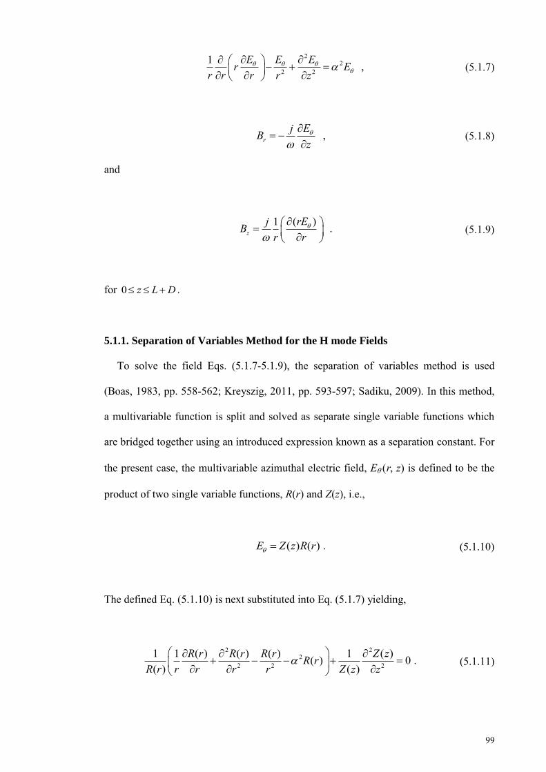
99

22

2 2

1 ,E E Er Er r r r z

(5.1.7)

,rEjBz

(5.1.8)

and

( )1 .zrEjB

r r

(5.1.9)

for 0 z L D .

5.1.1. Separation of Variables Method for the H mode Fields

To solve the field Eqs. (5.1.7-5.1.9), the separation of variables method is used

(Boas, 1983, pp. 558-562; Kreyszig, 2011, pp. 593-597; Sadiku, 2009). In this method,

a multivariable function is split and solved as separate single variable functions which

are bridged together using an introduced expression known as a separation constant. For

the present case, the multivariable azimuthal electric field, Erz is defined to be the

product of two single variable functions, R(r) and Z(z), i.e.,

( ) ( ) .E Z z R r (5.1.10)

The defined Eq. (5.1.10) is next substituted into Eq. (5.1.7) yielding,

2 22

2 2 2

1 1 ( ) ( ) ( ) 1 ( )( ) 0 .( ) ( )

R r R r R r Z zR rR r r r r r Z z z

(5.1.11)

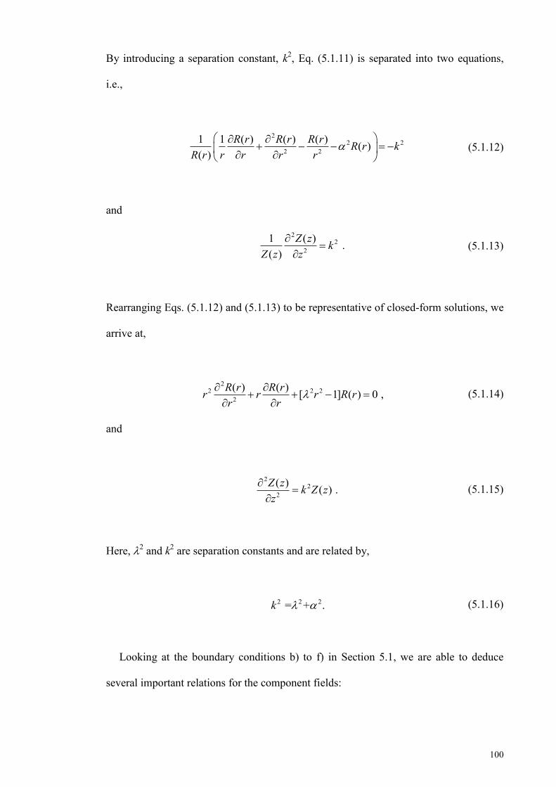
100

By introducing a separation constant, k2, Eq. (5.1.11) is separated into two equations,

i.e.,

22 2

2 2

1 1 ( ) ( ) ( ) ( )( )

R r R r R r R r kR r r r r r

(5.1.12)

and

22

2

1 ( ) .( )

Z z kZ z z

(5.1.13)

Rearranging Eqs. (5.1.12) and (5.1.13) to be representative of closed-form solutions, we

arrive at,

22 2 2

2

( ) ( ) [ 1] ( ) 0 ,R r R rr r r R rr r

(5.1.14)

and

22

2

( ) ( ) .Z z k Z zz

(5.1.15)

Here, 2 and k2 are separation constants and are related by,

2 2 2 = + .k (5.1.16)

Looking at the boundary conditions b) to f) in Section 5.1, we are able to deduce

several important relations for the component fields:

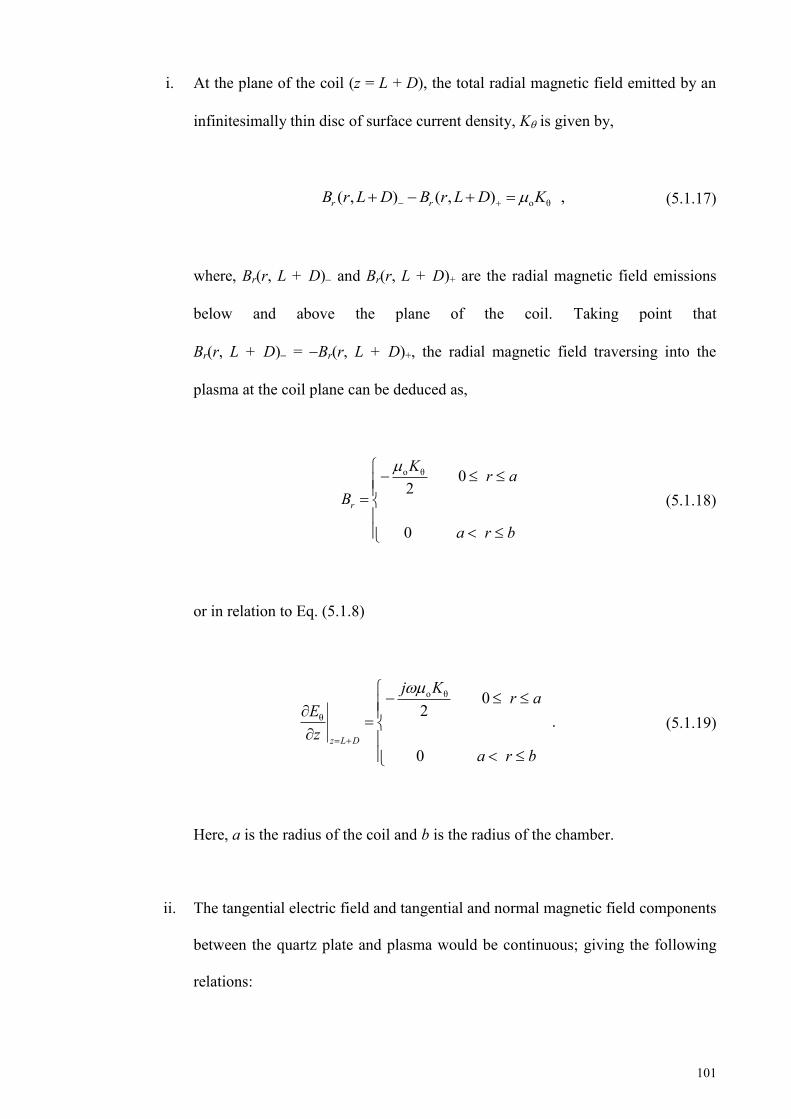
101

i. At the plane of the coil (z = L + D), the total radial magnetic field emitted by an

infinitesimally thin disc of surface current density, K is given by,

o θ( , ) ( , ) ,r rB r L D B r L D K (5.1.17)

where, Br(r, L + D) and Br(r, L + D)+ are the radial magnetic field emissions

below and above the plane of the coil. Taking point that

Br(r, L + D) = Br(r, L + D)+, the radial magnetic field traversing into the

plasma at the coil plane can be deduced as,

o θ 0 2

0

r

K r aB

a r b

(5.1.18)

or in relation to Eq. (5.1.8)

o θ

θ

0 2

.

0 z L D

j K r aEz

a r b

(5.1.19)

Here, a is the radius of the coil and b is the radius of the chamber.

ii. The tangential electric field and tangential and normal magnetic field components

between the quartz plate and plasma would be continuous; giving the following

relations:

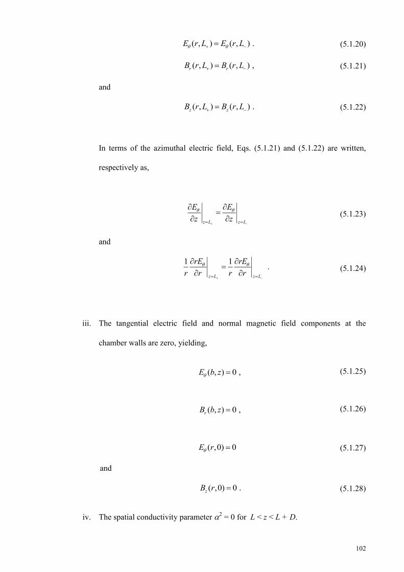
102

( , ) ( , ) .E r L E r L (5.1.20)

( , ) ( , ) ,r rB r L B r L (5.1.21)

and

( , ) ( , ) .z zB r L B r L (5.1.22)

In terms of the azimuthal electric field, Eqs. (5.1.21) and (5.1.22) are written,

respectively as,

z L z L

E Ez z

(5.1.23)

and

1 1 .z L z L

rE rEr r r r

(5.1.24)

iii. The tangential electric field and normal magnetic field components at the

chamber walls are zero, yielding,

( , ) 0 ,E b z (5.1.25)

( , ) 0 ,rB b z (5.1.26)

( ,0) 0 E r

and

(5.1.27)

( ,0) 0 .zB r (5.1.28)

iv. The spatial conductivity parameter 2 = 0 for L < z < L + D.

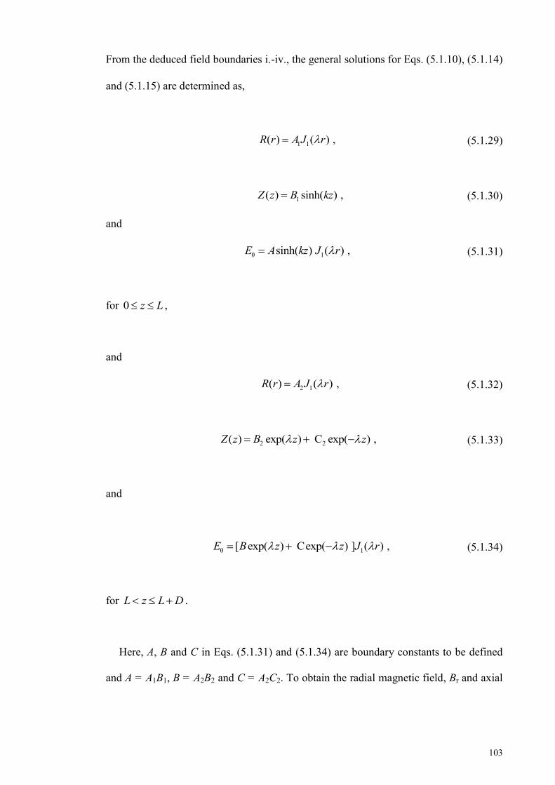
103

From the deduced field boundaries i.-iv., the general solutions for Eqs. (5.1.10), (5.1.14)

and (5.1.15) are determined as,

1 1( ) ( ) ,R r A J r (5.1.29)

1( ) sinh( ) ,Z z B kz (5.1.30)

and

θ 1sinh( ) ( ) ,E A kz J r (5.1.31)

for 0 z L ,

and

2 1( ) ( ) , R r A J r (5.1.32)

2 2( ) exp( ) C exp( ) ,Z z B z z (5.1.33)

and

θ 1[ exp( ) Cexp( ) ] ( ) ,E B z z J r (5.1.34)

for L z L D .

Here, A, B and C in Eqs. (5.1.31) and (5.1.34) are boundary constants to be defined

and A = A1B1, B = A2B2 and C = A2C2. To obtain the radial magnetic field, Br and axial

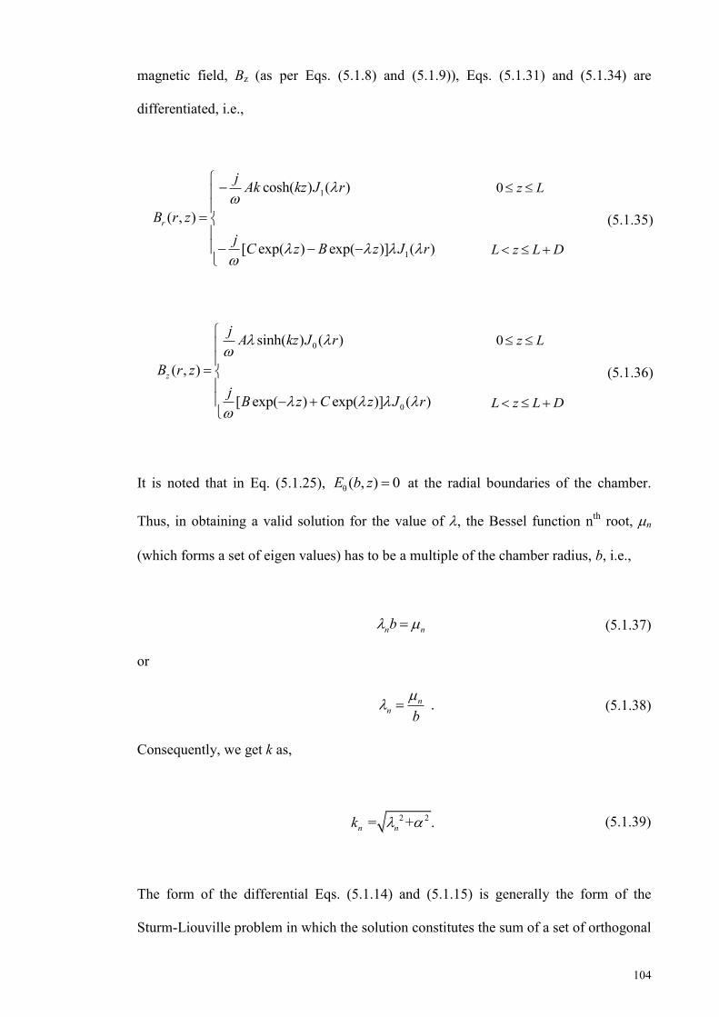
104

magnetic field, Bz (as per Eqs. (5.1.8) and (5.1.9)), Eqs. (5.1.31) and (5.1.34) are

differentiated, i.e.,

1

1

cosh( ) ( )

( , )

[ exp( ) exp( )] ( )

r

j Ak kz J r

B r zj C z B z J r

0 z L

L z L D

(5.1.35)

0

0

sinh( ) ( )

( , )

[ exp( ) exp( )] ( )

z

j A kz J r

B r zj B z C z J r

0 z L

L z L D

(5.1.36)

It is noted that in Eq. (5.1.25), θ ( , ) 0E b z at the radial boundaries of the chamber.

Thus, in obtaining a valid solution for the value of , the Bessel function nth root, n

(which forms a set of eigen values) has to be a multiple of the chamber radius, b, i.e.,

n nb (5.1.37)

or

.nn b

(5.1.38)

Consequently, we get k as,

2 2 = + .n nk (5.1.39)

The form of the differential Eqs. (5.1.14) and (5.1.15) is generally the form of the

Sturm-Liouville problem in which the solution constitutes the sum of a set of orthogonal

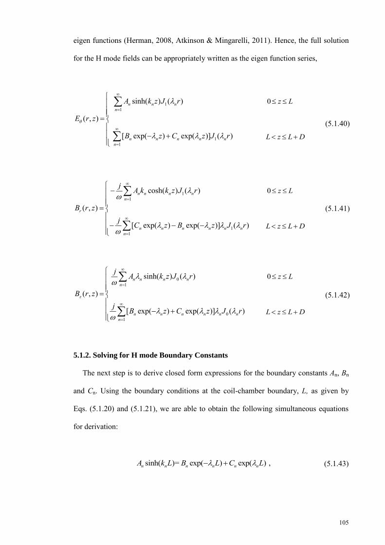
105

eigen functions (Herman, 2008, Atkinson & Mingarelli, 2011). Hence, the full solution

for the H mode fields can be appropriately written as the eigen function series,

11

11

sinh( ) ( )

( , )

[ exp( ) exp( )] ( )

n n nn

n n n n nn

A k z J r

E r z

B z C z J r

0 z L

L z L D

(5.1.40)

11

11

cosh( ) ( )

( , )

[ exp( ) exp( )] ( )

n n n nn

r

n n n n n nn

j A k k z J r

B r zj C z B z J r

0 z L

L z L D

(5.1.41)

01

01

sinh( ) ( )

( , )

[ exp( ) exp( )] ( )

n n n nn

z

n n n n n nn

j A k z J r

B r zj B z C z J r

0 z L

L z L D

(5.1.42)

5.1.2. Solving for H mode Boundary Constants

The next step is to derive closed form expressions for the boundary constants An, Bn

and Cn. Using the boundary conditions at the coil-chamber boundary, L, as given by

Eqs. (5.1.20) and (5.1.21), we are able to obtain the following simultaneous equations

for derivation:

sinh( )= exp( ) exp( ) ,n n n n n nA k L B L C L (5.1.43)

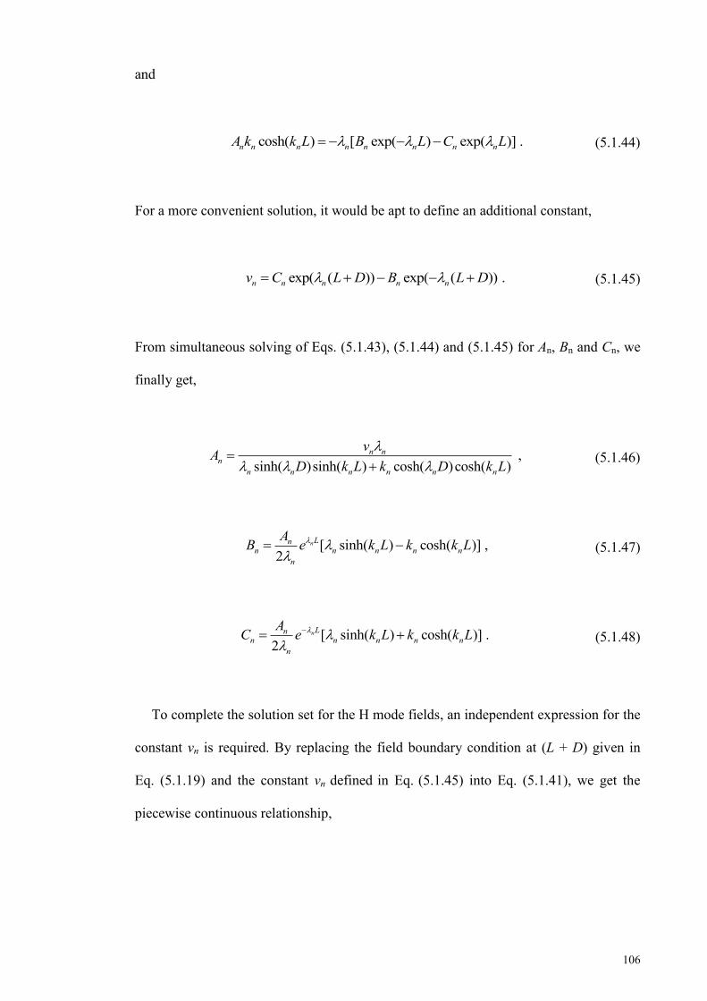
106

and

cosh( ) [ exp( ) exp( )] .n n n n n n n nA k k L B L C L (5.1.44)

For a more convenient solution, it would be apt to define an additional constant,

exp( ( )) exp( ( )) .n n n n nv C L D B L D (5.1.45)

From simultaneous solving of Eqs. (5.1.43), (5.1.44) and (5.1.45) for An, Bn and Cn, we

finally get,

,sinh( )sinh( ) cosh( )cosh( )

n nn

n n n n n n

vAD k L k D k L

(5.1.46)

[ sinh( ) cosh( )] ,2

nLnn n n n n

n

AB e k L k k L

(5.1.47)

[ sinh( ) cosh( )] .2

nLnn n n n n

n

AC e k L k k L

(5.1.48)

To complete the solution set for the H mode fields, an independent expression for the

constant vn is required. By replacing the field boundary condition at (L + D) given in

Eq. (5.1.19) and the constant vn defined in Eq. (5.1.45) into Eq. (5.1.41), we get the

piecewise continuous relationship,

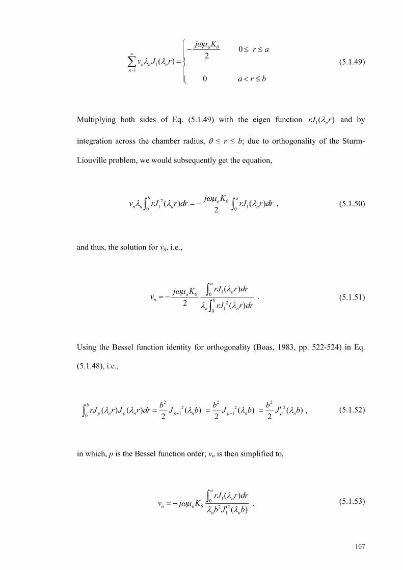
107

o

11

0 2

( )

0

n n nn

j K r av J r

a r b

(5.1.49)

Multiplying both sides of Eq. (5.1.49) with the eigen function 1( )nrJ r and by

integration across the chamber radius, ≤ r ≤ b; due to orthogonality of the Sturm-

Liouville problem, we would subsequently get the equation,

2 o1 10 0

( ) ( ) ,2

b a

n n n nj Kv rJ r dr rJ r dr

(5.1.50)

and thus, the solution for vn, i.e.,

1o 0

210

( ) .

2 ( )

a

nn b

n n

rJ r drj KvrJ r dr

(5.1.51)

Using the Bessel function identity for orthogonality (Boas, 1983, pp. 522-524) in Eq.

(5.1.48), i.e.,

2 2 22 2 2

1 10( ) ( ) ( ) ( ) ( ) ,

2 2 2b

p n p n p n p n p nb b brJ r J r dr J b J b J b

(5.1.52)

in which, p is the Bessel function order; vn is then simplified to,

10o 2 2

1

( ) .

( )

a

nn

n n

rJ r drv j K

b J b

(5.1.53)

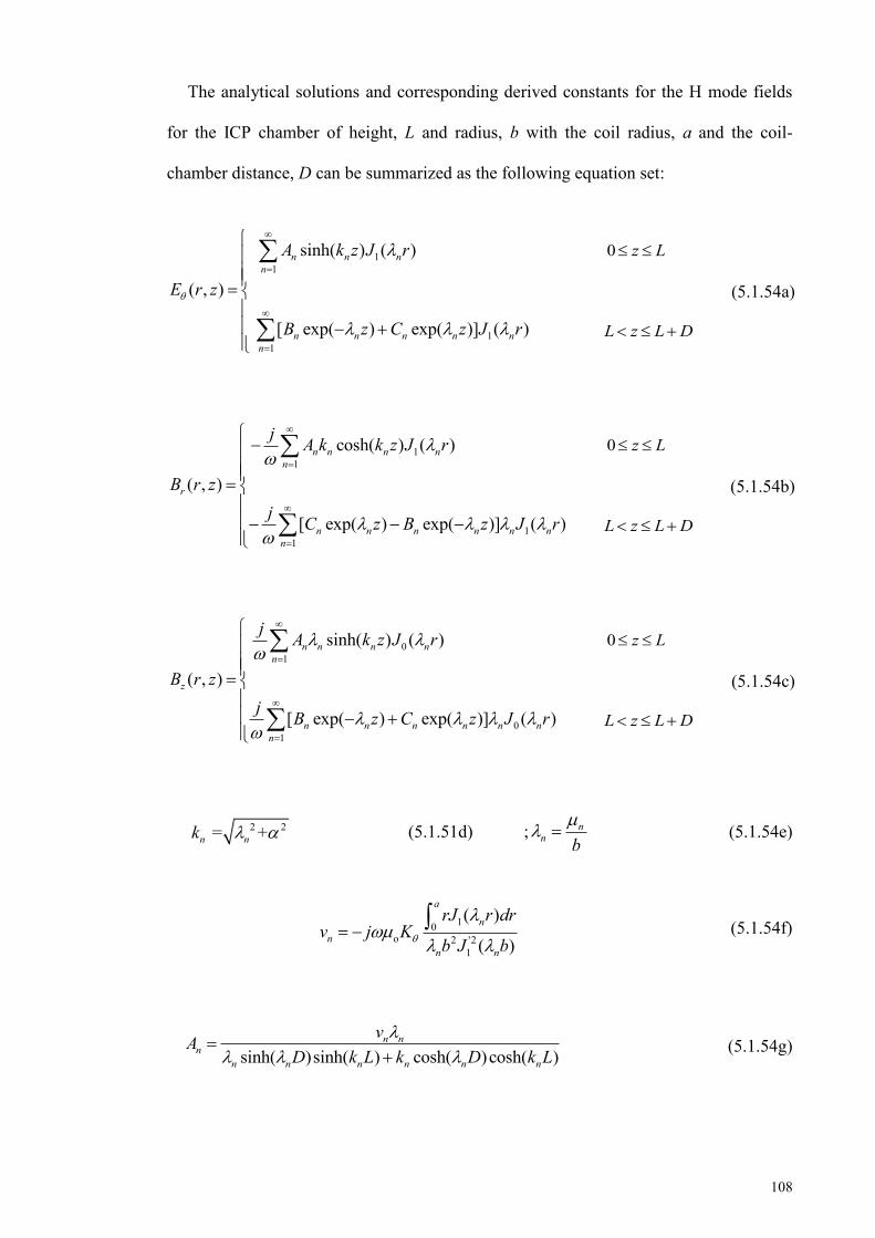
108

The analytical solutions and corresponding derived constants for the H mode fields

for the ICP chamber of height, L and radius, b with the coil radius, a and the coil-

chamber distance, D can be summarized as the following equation set:

11

11

sinh( ) ( )

( , )

[ exp( ) exp( )] ( )

n n nn

n n n n nn

A k z J r

E r z

B z C z J r

0 z L

L z L D

(5.1.54a)

11

11

cosh( ) ( )

( , )

[ exp( ) exp( )] ( )

n n n nn

r

n n n n n nn

j A k k z J r

B r zj C z B z J r

0 z L

L z L D

(5.1.54b)

01

01

sinh( ) ( )

( , )

[ exp( ) exp( )] ( )

n n n nn

z

n n n n n nn

j A k z J r

B r zj B z C z J r

0 z L

L z L D

(5.1.54c)

2 2 = +n nk (5.1.51d) ; nn b

(5.1.54e)

10o 2 '2

1

( )

( )

a

nn

n n

rJ r drv j K

b J b

(5.1.54f)

sinh( )sinh( ) cosh( )cosh( )n n

nn n n n n n

vAD k L k D k L

(5.1.54g)

109

exp( )[ sinh( ) cosh( )]2

nn n n n n n

n

AB L k L k k L

(5.1.54h)

exp( )[ sinh( ) cosh( )]2

nn n n n n n

n

AC L k L k k L

(5.1.54i)

A MATLAB code for solving the analytical H mode fields (equation set (5.1.54)) can be

found in Appendix C.

5.2. Numerical H mode fields

The numerical H mode fields are solved using Eqs. (5.1.7-5.1.9) with the finite

difference method (Sadiku, 2009; Zhou, 1993; Salon & Chari, 2000). One of the

advantages of solving the fields numerically is the ability to input spatially resolved (-r

and –z varying) plasma parameters such as electron density, ne (r, z), electron

temperature, Te (r, z) and neutral gas temperature, Tn (r, z) which will give a better

theoretical visualization of the electromagnetic fields in the laboratory reactor. The

actual chamber dimensions can also be straightforwardly modeled by this method.

In the finite difference method, the plasma chamber is divided into a 2 dimensional

grid of equally spaced cells with a radial spacing, Δr and axial spacing, Δz. Δr and Δz

are chosen to be small enough such that,

, 1, , 1, ,2

n m n mE E Er r

(5.2.1)

2, 1, , , , 1,

2 2

2 ,

( )n m n m n mE E E E

r r

(5.2.2)

110

, , 1 , , 1 ,2

n m n mE E Ez z

(5.2.3)

and

2, , 1 , , , , 1

2 2

2 .

( )n m n m n mE E E E

z z

(5.2.4)

Here, the n and m subscripts represent the radial and axial positions of the calculated

field points on the grid. Rewriting Eqs. (5.1.7-5.1.9) in finite difference notation, we

get,

, 1, , , 1 , 1, , , , 1, , ,2 2

, ,

, , 1 , , , , 1 2, , ,2

212 ( )

2 ( , ) ,

( )

n m n m n m n m n m n m

n m n m

n m n m n mn m n m

E E E E E Er r r r

E E Er z E

z

(5.2.5)

, , 1 , , 1, , ,

2n m n m

r n m

E EjBz

(5.2.6)

and

1, , 1, 1, , 1,, ,

,

1 .2

n m n m n m n mz n m

n m

r E r EjBr r

(5.2.7)

2, ( , )n m r z represents the radially and axially resolved spatial conductivity parameter for

the grid position (n, m). To avoid singularity for Eqs. (5.2.5) and (5.2.7) as r approaches

zero, i.e., r→0, L'Hôpital's rule was applied to Eqs. (5.1.7) and (5.1.9) for calculations

at r 0, yielding the reduced finite difference solutions,

111

, 1, , , , 1,2

, , 1 , , , , 1 2, , ,2

232 ( )

2 ( , ) ,

( )

n m n m n m

n m n m n mn m n m

E E Er

E E Er z E

z

(5.2.8)

and

, 1, , , , 1,, , 2

22 .( )

n m n m n mz n m

E E EjBr

(5.2.9)

In a spatially resolved form, the spatial conductivity parameter is represented by a

spatially varying electron density, ne (r, z) and effective collision frequency, eff (r, z)

i.e.,

22 o e

e eff

( , )( , ) .1 ( , )

n r z er zm j r z

(5.2.10)

5.2.1 Calculation of Effective Collision Frequency, eff (r, z)

The effective electron collision frequency, eff (r, z) consists of the sum of most

frequent particle collisions occurring in the plasma. For the present setup, the sum of the

three largest collision frequencies were used to estimate eff (r, z), i.e., the electron

neutral collision frequency, en, electron ion collision frequency, ei, and stochastic

collision frequency, st (Gudmundsson & Lieberman, 1998; Maurice, 2003, pp. 74-75).

eff (r, z) is thus, denoted as,

eff en ei st( , )r z (5.2.11)

112

The electron-neutral collision frequency, en is obtained from the integral between the

argon atom collision frequency and EEDF, i.e. (Lister, Li & Godyak, 1996),

13 2

en eff 0c

3 ( ) ,2 ( )

dfj dj d

(5.2.12)

with being the electron energy in J, eff being the effective drive frequency in Hz, ,c

() is the collision frequency term for argon gas and f() is the EEDF. For simplicity of

calculation, a Maxwellian EEDF is used and is defined as,

),(exp

),(12)(

e23

e zrTzreTf

(5.2.13)

where, Te (r, z) is the electron temperature in eV. The collision frequency term,c () of

argon gas is given by,

ecgc

2)(),()(mezrn

(5.2.14)

Here, ng (r, z) is the neutral gas density of the plasma in m3 and c () is the collision

cross section of argon gas in m2 taken from Hayashi (1981); Appendix E, Table E.1.

ng (r, z) for this model is deduced from the ideal gas law,

g e B ni B, / , /( , .) nn r z P p k T r z P k rp T z (5.2.15)

P, pi and pe are the argon filling pressure, ion pressure and electron pressure,

respectively in Pa, kB is the Boltzmann constant in JK1 and Tn (r, z) is the neutral gas

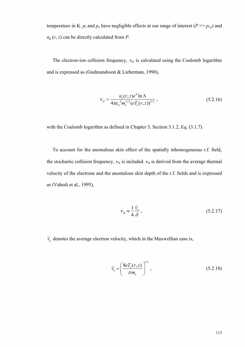
113

temperature in K. pi and pe have negligible effects at our range of interest (P >> pi,e) and

ng (r, z) can be directly calculated from P.

The electron-ion collision frequency, ei is calculated using the Coulomb logarithm

and is expressed as (Gudmundsson & Lieberman, 1998),

4e

ei 2 1/2 3/2o e e

( , ) ln ,4 ( ( , ))

n r z em eT r z

(5.2.16)

with the Coulomb logarithm as defined in Chapter 3, Section 3.1.2, Eq. (3.1.7).

To account for the anomalous skin effect of the spatially inhomogeneous r.f. field,

the stochastic collision frequency, st is included. st is derived from the average thermal

velocity of the electrons and the anomalous skin depth of the r.f. fields and is expressed

as (Vahedi et al., 1995),

est

1 ,4

v

(5.2.17)

ev denotes the average electron velocity, which in the Maxwellian case is,

1/2

ee

e

8 ( , ) ,eT r zvm

(5.2.18)

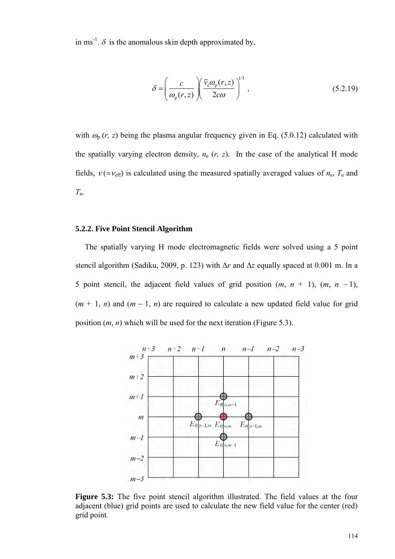
114

in ms-1. is the anomalous skin depth approximated by,

1/3e p

p

( , ),

( , ) 2v r zc

r z c

(5.2.19)

with p (r, z) being the plasma angular frequency given in Eq. (5.0.12) calculated with

the spatially varying electron density, ne (r, z). In the case of the analytical H mode

fields, eff) is calculated using the measured spatially averaged values of ne, Te and

Tn.

5.2.2. Five Point Stencil Algorithm

The spatially varying H mode electromagnetic fields were solved using a 5 point

stencil algorithm (Sadiku, 2009, p. 123) with Δr and Δz equally spaced at 0.001 m. In a

5 point stencil, the adjacent field values of grid position (m, n + 1), (m, n 1),

(m + 1, n) and (m 1, n) are required to calculate a new updated field value for grid

position (m, n) which will be used for the next iteration (Figure 5.3).

Figure 5.3: The five point stencil algorithm illustrated. The field values at the four adjacent (blue) grid points are used to calculate the new field value for the center (red) grid point.

115

This cycle of calculations are repeated until the field values remain unchanged between

successive iterations within an acceptable magnitude of error, i.e. convergence. The

calculations are bounded within the chamber dimensions using the following boundary

conditions:

i. The walls of the chamber are assumed to be infinitely conducting, such that all

fields at the walls are equal to zero.

ii. The radial magnetic fields at the coil surface (L + D) for the coil radius of

–a ≤ r ≤ a is constant and is given by,

o θ .2rKB

(5.2.20)

A flowchart of the program algorithm is shown in Figure 5.4.

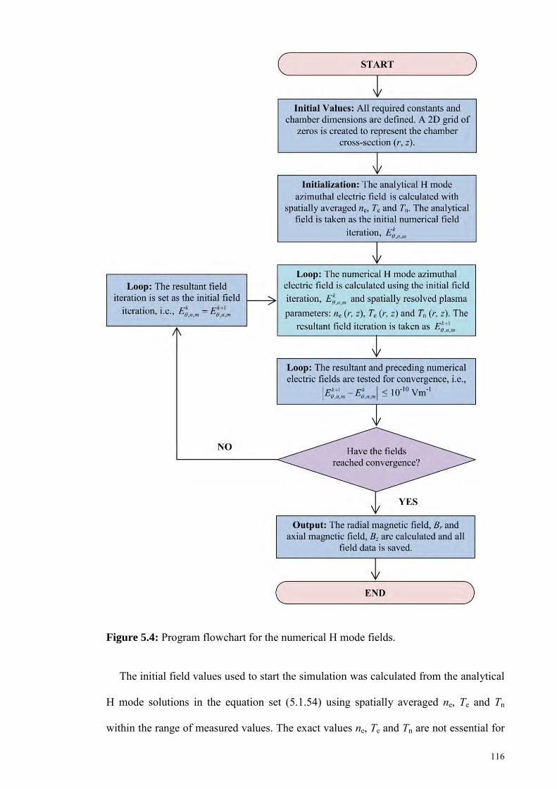
116

Figure 5.4: Program flowchart for the numerical H mode fields.

The initial field values used to start the simulation was calculated from the analytical

H mode solutions in the equation set (5.1.54) using spatially averaged ne, Te and Tn

within the range of measured values. The exact values ne, Te and Tn are not essential for

117

accuracy, however, closer estimates to expected values would yield faster convergence.

The convergence point for the algorithm is set at a maximum deviation of 1010 T

between successive iterations.

5.3. Analytical E mode fields

For deriving the analytical E mode fields, a similar set of assumptions and boundary

conditions as the H mode fields were applied to Eqs. (5.0.7-5.0.12):

a) The coil (at a ≤ r ≤ a) is assumed to be an infinitely thin disc with an uniform

radial electric field, Eo of magnitude,

po .

VE

a (5.3.1)

where Vp is the peak coil current in V and a is the coil radius in m.

b) The chamber is an azimuthally symmetric cylinder of radius, b and effective

height, L with a coil radius of a. The coil-chamber spacing is D.

c) The chamber (from boundaries –b < r < b and 0 < z < L) has a uniform electron

density, ne, collision frequency, and electron temperature, Te. Externally, these

parameters are equal to zero.

d) At the boundaries between the chamber walls and the plasma, the normal

magnetic fields and tangential electric fields are equal to zero.

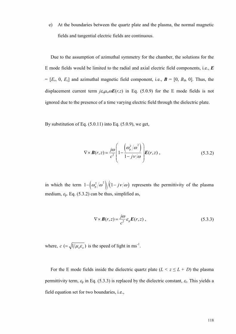
118

e) At the boundaries between the quartz plate and the plasma, the normal magnetic

fields and tangential electric fields are continuous.

Due to the assumption of azimuthal symmetry for the chamber, the solutions for the

E mode fields would be limited to the radial and axial electric field components, i.e., E

= [Er, 0, Ez] and azimuthal magnetic field component, i.e., B = [0, B, 0]. Thus, the

displacement current term jooE(r,z) in Eq. (5.0.9) for the E mode fields is not

ignored due to the presence of a time varying electric field through the dielectric plate.

By substitution of Eq. (5.0.11) into Eq. (5.0.9), we get,

22p

2( , ) 1 ( , ) ,1

jr z r zc j

B E (5.3.2)

in which the term

22p1 1 j represents the permittivity of the plasma

medium, p. Eq. (5.3.2) can be thus, simplified as,

p2( , ) ( , ) ,jr z r zc B E (5.3.3)

where, o o ( 1 )c is the speed of light in ms-1.

For the E mode fields inside the dielectric quartz plate (L < z ≤ L + D) the plasma

permittivity term,p in Eq. (5.3.3) is replaced by the dielectric constant,r. This yields a

field equation set for two boundaries, i.e.,

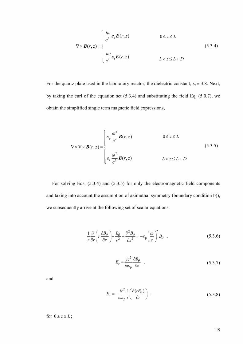
119

p2

r2

( , )

( , )

( , )

j r zc

r zj r zc

E

B

E

0 z L

L z L D

(5.3.4)

For the quartz plate used in the laboratory reactor, the dielectric constant, r 3.8. Next,

by taking the curl of the equation set (5.3.4) and substituting the field Eq. (5.0.7), we

obtain the simplified single term magnetic field expressions,

2

p 2

2

r 2

( , )

( , )

( , )

r zc

r z

r zc

B

B

B

0 z L

L z L D

(5.3.5)

For solving Eqs. (5.3.4) and (5.3.5) for only the electromagnetic field components

and taking into account the assumption of azimuthal symmetry (boundary condition b)),

we subsequently arrive at the following set of scalar equations:

22

p2 2 ,1 B B Br Br r r cr z

(5.3.6)

2

p ,r

BjcEz

(5.3.7)

and

2

p

(1 )

.zrBjcE

r r

(5.3.8)

for 0 z L ;

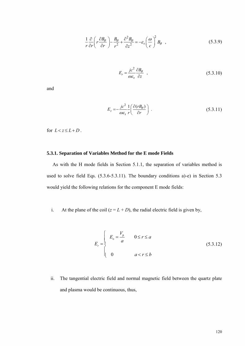
120

22

r2 2 ,1 B B Br Br r r cr z

(5.3.9)

2

r ,r

BjcEz

(5.3.10)

and

2

r

(1 )

.zrBjcE

r r

(5.3.11)

for L z L D .

5.3.1. Separation of Variables Method for the E mode Fields

As with the H mode fields in Section 5.1.1, the separation of variables method is

used to solve field Eqs. (5.3.6-5.3.11). The boundary conditions a)-e) in Section 5.3

would yield the following relations for the component E mode fields:

i. At the plane of the coil (z = L + D), the radial electric field is given by,

po 0

0

r

VE r a

aE

a r b

(5.3.12)

ii. The tangential electric field and normal magnetic field between the quartz plate

and plasma would be continuous, thus,

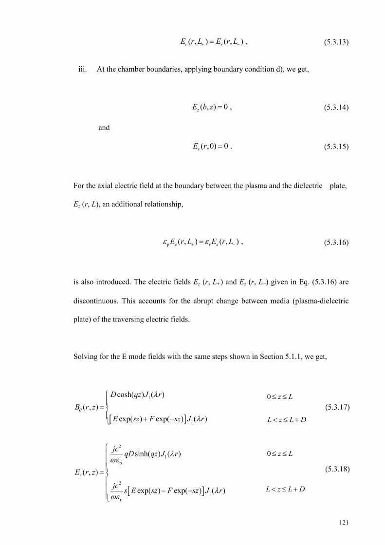
121

( , ) ( , ) ,r rE r L E r L (5.3.13)

iii. At the chamber boundaries, applying boundary condition d), we get,

( , ) 0 ,zE b z (5.3.14)

and

( ,0) 0 .rE r (5.3.15)

For the axial electric field at the boundary between the plasma and the dielectric plate,

Ez (r, L), an additional relationship,

p r( , ) ( , ) ,z zE r L E r L (5.3.16)

is also introduced. The electric fields Ez (r, L+) and Ez (r, L) given in Eq. (5.3.16) are

discontinuous. This accounts for the abrupt change between media (plasma-dielectric

plate) of the traversing electric fields.

Solving for the E mode fields with the same steps shown in Section 5.1.1, we get,

1

1

cosh( ) ( ) ( , )

exp( ) exp( ) ( )

D qz J rB r z

E sz F sz J r

0 z L

L z L D (5.3.17)

2

1

2

r

1p

sinh( ) ( )

( , )

exp( ) exp( ) ( )

r

qz J r

E r z

E sz F sz J

jc qD

jc s r

0 z L

L z L D

(5.3.18)

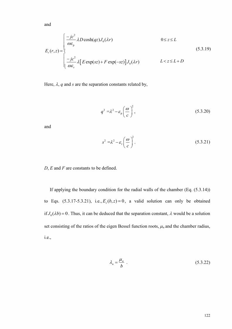
122

and

2

0

0

p

2

r

cosh( ) ( )

( , )

exp( ) exp( ) ( )

r

qz J r

E r z

E sz F

jc D

jc sz J r

0 z L

L z L D

(5.3.19)

Here, , q and s are the separation constants related by,

22

p2 = ,

cq

(5.3.20)

and

22

r2 = .

cs

(5.3.21)

D, E and F are constants to be defined.

If applying the boundary condition for the radial walls of the chamber (Eq. (5.3.14))

to Eqs. (5.3.17-5.3.21), i.e., ( , ) 0zE b z , a valid solution can only be obtained

if 0( ) 0J b . Thus, it can be deduced that the separation constant, would be a solution

set consisting of the ratios of the eigen Bessel function roots,n and the chamber radius,

i.e.,

.nn b

(5.3.22)

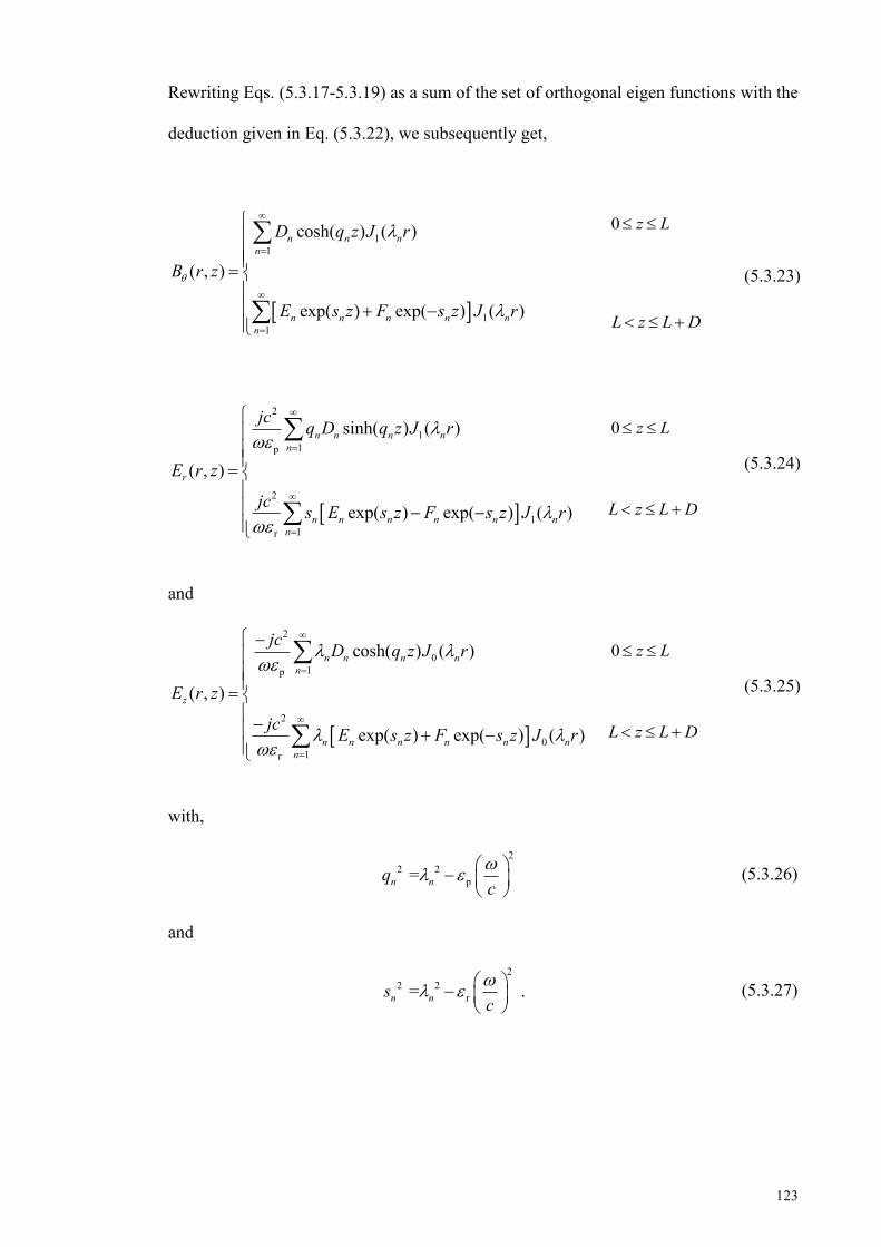
123

Rewriting Eqs. (5.3.17-5.3.19) as a sum of the set of orthogonal eigen functions with the

deduction given in Eq. (5.3.22), we subsequently get,

11

11

cosh( ) ( )

( , )

exp( ) exp( ) ( )

n n nn

n n n n nn

D q z J r

B r z

E s z F s z J r

0 z L

L z L D

(5.3.23)

2

p

2

r

11

11

sinh( ) ( )

( , )

exp( ) exp( ) ( )

n nn

r

n n

n n

n n n nn

q z J r

E r z

E s z F s z J

jc q D

jc s r

0 z L

L z L D

(5.3.24)

and

01

0

2

r 1

2

p

cosh( ) ( )

( , )

exp( ) exp( ) ( )

n n nn

z

n n n n n n

n

n

q z J r

E r z

E s z

j

F s z J r

c D

jc

0 z L

L z L D

(5.3.25)

with,

p

22 2 =n nq

c

(5.3.26)

and

r

22 2 = .n n c

s

(5.3.27)

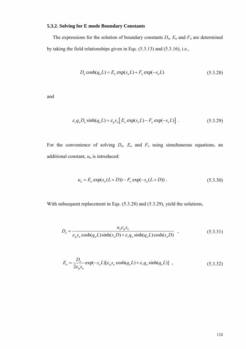
124

5.3.2. Solving for E mode Boundary Constants

The expressions for the solution of boundary constants Dn, En and Fn are determined

by taking the field relationships given in Eqs. (5.3.13) and (5.3.16), i.e.,

cosh( ) exp( ) exp( )n n n n nn q L E s L F s LD (5.3.28)

and

r psinh( ) exp( ) exp( ) .n n nn n n n nq L E s L F sq D s L (5.3.29)

For the convenience of solving Dn, En and Fn using simultaneous equations, an

additional constant, un is introduced:

exp( ( )) exp( ( )) .n n n n nu E s L D F s L D (5.3.30)

With subsequent replacement in Eqs. (5.3.28) and (5.3.29), yield the solutions,

p

p r

,cosh( )sinh( ) sinh( )cosh( )

n nn

n n n n n n

u sD

s q L s D q q L s D

(5.3.31)

p rp

exp( )[ cosh( ) sinh( )] ,2

nn n n n n n

n

DE s L s q L q q Ls

(5.3.32)

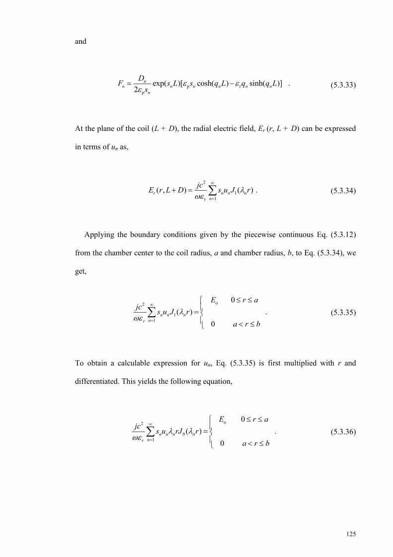
125

and

p rp

exp( )[ cosh( ) sinh( )] .2

nn n n n n n

n

DF s L s q L q q Ls

(5.3.33)

At the plane of the coil (L + D), the radial electric field, Er (r, L + D) can be expressed

in terms of un as,

2

11

r

( )( , ) .r n nn

nJjcE r L D s u r

(5.3.34)

Applying the boundary conditions given by the piecewise continuous Eq. (5.3.12)

from the chamber center to the coil radius, a and chamber radius, b, to Eq. (5.3.34), we

get,

o2

11

0( ) .

0 nn n

nr

jc s uE r a

J ra r b

(5.3.35)

To obtain a calculable expression for un, Eq. (5.3.35) is first multiplied with r and

differentiated. This yields the following equation,

o2

10

0( ) .

0 n n

nrn n

E r aJ rjc

as u r

r b

(5.3.36)

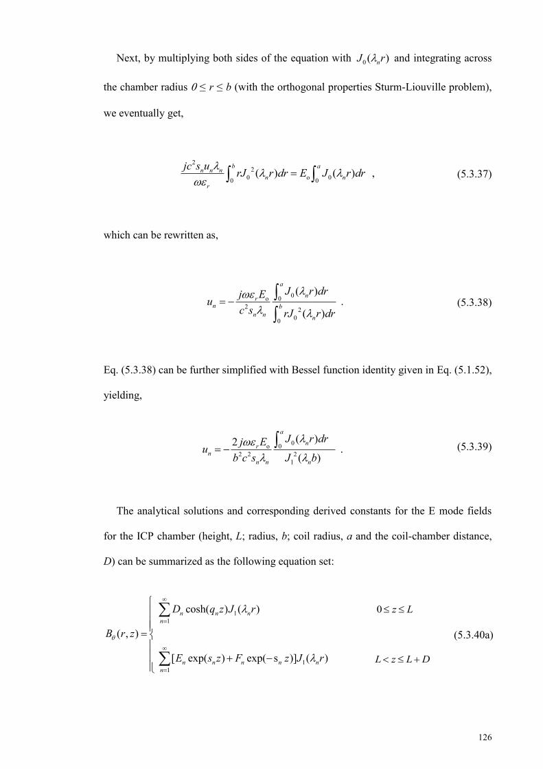
126

Next, by multiplying both sides of the equation with 0 ( ) nJ r and integrating across

the chamber radius ≤ r ≤ b (with the orthogonal properties Sturm-Liouville problem),

we eventually get,

20 o 00 0

2

( ) ( ) ,b an

n nn n

r

J r drjc s E J ru r r d

(5.3.37)

which can be rewritten as,

0o 0

20

2

0

( ) .

( )

a

n

bn

rn

n n

J r drE

J r

j

r dc s ru

(5.3.38)

Eq. (5.3.38) can be further simplified with Bessel function identity given in Eq. (5.1.52),

yielding,

0o 0222

1

( ) 2 .( )

a

n

n

rn

nn

juc

J r drEsb J b

(5.3.39)

The analytical solutions and corresponding derived constants for the E mode fields

for the ICP chamber (height, L; radius, b; coil radius, a and the coil-chamber distance,

D) can be summarized as the following equation set:

11

11

cosh( ) ( )

( , )

[ exp( ) exp( s )] ( )

n n nn

n n n n nn

D q z J r

B r z

E s z F z J r

0 z L

L z L D

(5.3.40a)

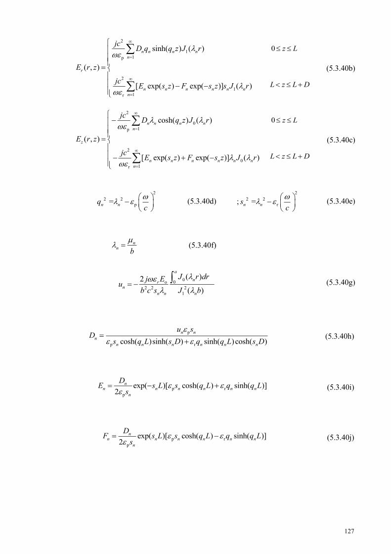
127

2

11p

2

11r

sinh( ) ( )

( , )

[ exp( ) exp( )] ( )

n n n nn

r

n n n n n nn

jc D q q z J r

E r z

jc E s z F s z s J r

0 z L

L z L D

(5.3.40b)

2

01p

2

01r

cosh( ) ( )

( , )

[ exp( ) exp( )] ( )

n n n nn

z

n n n n n nn

jc D q z J r

E r z

jc E s z F s z J r

0 z L

L z L D

(5.3.40c)

p

22 2 =n nq

c

(5.3.40d) ; r

22 2 = n n c

s

(5.3.40e)

nn b

(5.3.40f)

0o 02

122

( ) 2( )

r

n n nn

a

njuc

J r drEb J bs

(5.3.40g)

p

p rcosh( )sinh( ) sinh( )cosh( )n n

nn n n n n n

u sD

s q L s D q q L s D

(5.3.40h)

p rp

exp( )[ cosh( ) sinh( )]2

nn n n n n n

n

DE s L s q L q q Ls

(5.3.40i)

p rp

exp( )[ cosh( ) sinh( )]2

nn n n n n n

n

DF s L s q L q q Ls

(5.3.40j)

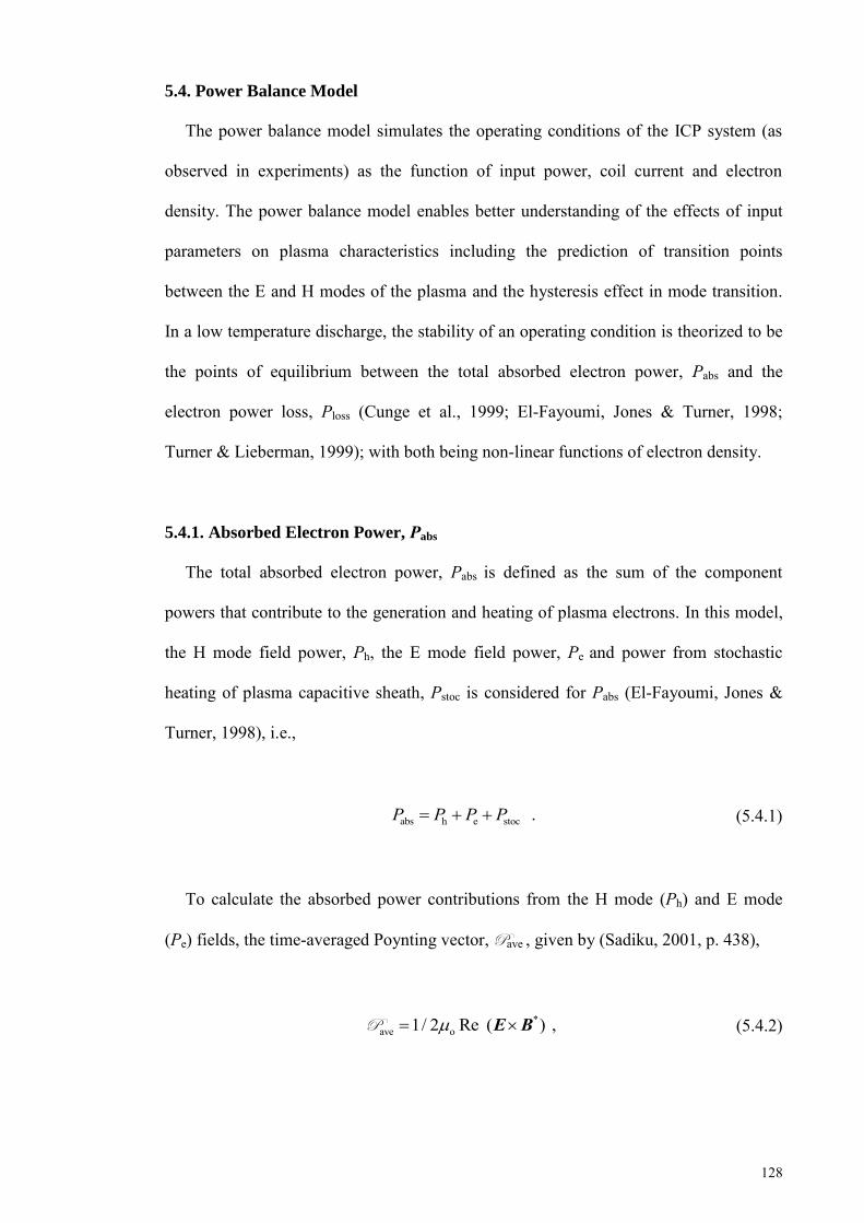
128

5.4. Power Balance Model

The power balance model simulates the operating conditions of the ICP system (as

observed in experiments) as the function of input power, coil current and electron

density. The power balance model enables better understanding of the effects of input

parameters on plasma characteristics including the prediction of transition points

between the E and H modes of the plasma and the hysteresis effect in mode transition.

In a low temperature discharge, the stability of an operating condition is theorized to be

the points of equilibrium between the total absorbed electron power, Pabs and the

electron power loss, Ploss (Cunge et al., 1999; El-Fayoumi, Jones & Turner, 1998;

Turner & Lieberman, 1999); with both being non-linear functions of electron density.

5.4.1. Absorbed Electron Power, Pabs

The total absorbed electron power, Pabs is defined as the sum of the component

powers that contribute to the generation and heating of plasma electrons. In this model,

the H mode field power, Ph, the E mode field power, Pe and power from stochastic

heating of plasma capacitive sheath, Pstoc is considered for Pabs (El-Fayoumi, Jones &

Turner, 1998), i.e.,

abs h e stoc .PP P P (5.4.1)

To calculate the absorbed power contributions from the H mode (Ph) and E mode

(Pe) fields, the time-averaged Poynting vector, Pave , given by (Sadiku, 2001, p. 438),

*ave o1/ 2 Re ( ) , E BP (5.4.2)

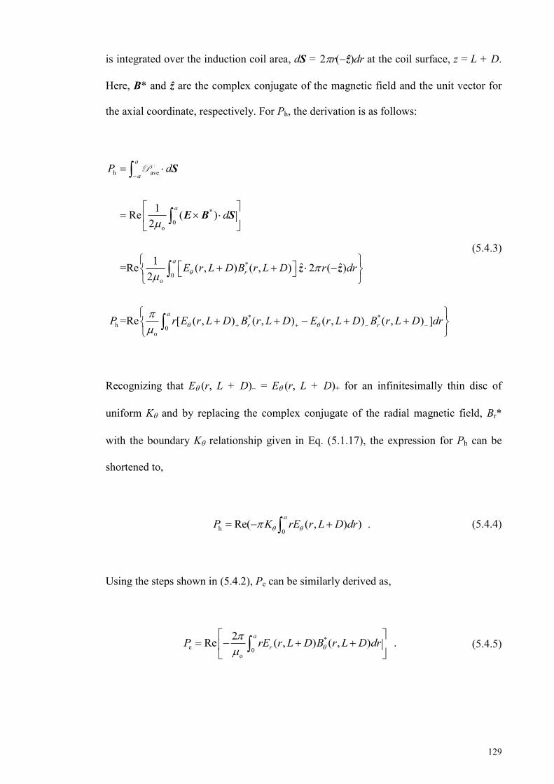
129

is integrated over the induction coil area, dS = 2rẑ)dr at the coil surface, z = L + D.

Here, B* and ẑ are the complex conjugate of the magnetic field and the unit vector for

the axial coordinate, respectively. For Ph, the derivation is as follows:

ave

0o

*

0o

* *

0o

h

h

1Re (2

1 ˆ ˆ=Re ( , ) ( , ) 2 (

)

)2

=Re [ ( , ) ( , ) ( , ) ( , ) ]

a

a

a

a

r

a

r r

P d

d

P

E r L D B r L D r dr

r E r L D B r L D E r L D B r L D dr

*

z z

S

E B S

P

(5.4.3)

Recognizing that E(r, L + D) = E(r, L + D)+ for an infinitesimally thin disc of

uniform K and by replacing the complex conjugate of the radial magnetic field, Br*

with the boundary K relationship given in Eq. (5.1.17), the expression for Ph can be

shortened to,

0h Re( ( , ) ) .a

K rE rP L D dr (5.4.4)

Using the steps shown in (5.4.2), Pe can be similarly derived as,

*e 0

o

2Re ( , ) ( , ) .a

rP rE r L D B r L D dr

(5.4.5)

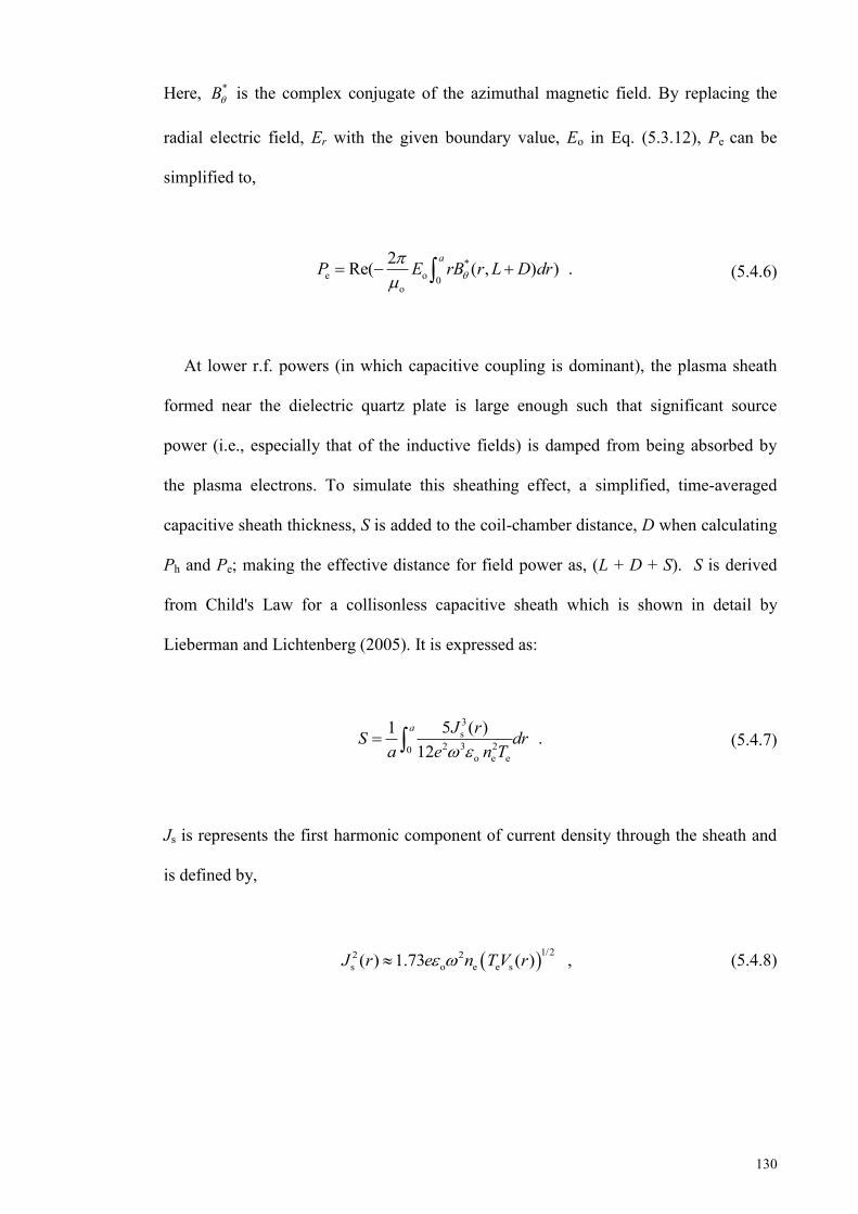
130

Here, *B is the complex conjugate of the azimuthal magnetic field. By replacing the

radial electric field, Er with the given boundary value, Eo in Eq. (5.3.12), Pe can be

simplified to,

*e o 0

o

2Re( ( , ) ) .a

E rB r LP D dr

(5.4.6)

At lower r.f. powers (in which capacitive coupling is dominant), the plasma sheath

formed near the dielectric quartz plate is large enough such that significant source

power (i.e., especially that of the inductive fields) is damped from being absorbed by

the plasma electrons. To simulate this sheathing effect, a simplified, time-averaged

capacitive sheath thickness, S is added to the coil-chamber distance, D when calculating

Ph and Pe; making the effective distance for field power as, (L + D + S). S is derived

from Child's Law for a collisonless capacitive sheath which is shown in detail by

Lieberman and Lichtenberg (2005). It is expressed as:

3s

2 3 20o e e

5 ( )1 .12

a J rS dra e n T

(5.4.7)

Js is represents the first harmonic component of current density through the sheath and

is defined by,

1/22 2

s o e e s ( ) 1.73 ( ) ,J r e n T V r (5.4.8)

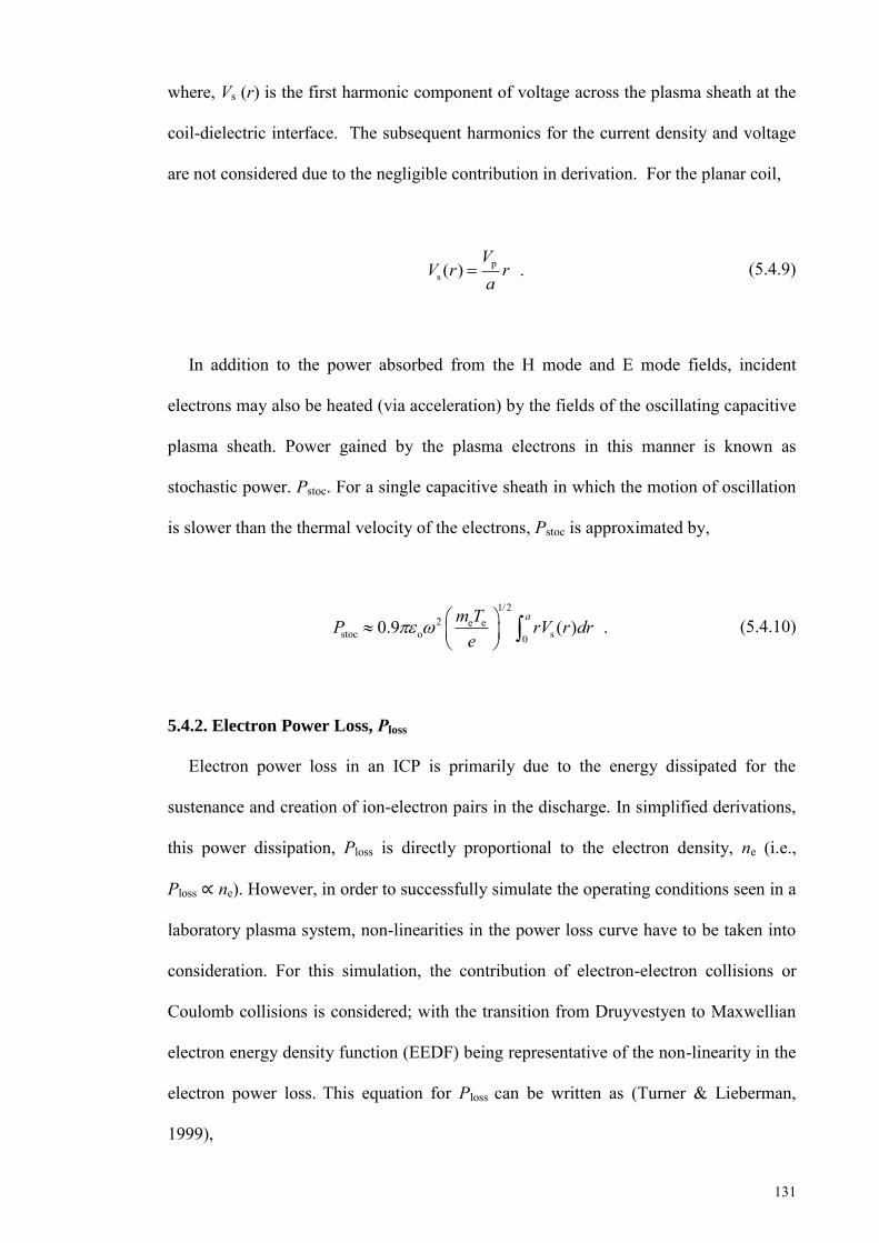
131

where, Vs (r) is the first harmonic component of voltage across the plasma sheath at the

coil-dielectric interface. The subsequent harmonics for the current density and voltage

are not considered due to the negligible contribution in derivation. For the planar coil,

ps ( ) .

VV r r

a (5.4.9)

In addition to the power absorbed from the H mode and E mode fields, incident

electrons may also be heated (via acceleration) by the fields of the oscillating capacitive

plasma sheath. Power gained by the plasma electrons in this manner is known as

stochastic power. Pstoc. For a single capacitive sheath in which the motion of oscillation

is slower than the thermal velocity of the electrons, Pstoc is approximated by,

1/22 e e

stoc o s0 0.9 ( ) .

am TP rV r dre

(5.4.10)

5.4.2. Electron Power Loss, Ploss

Electron power loss in an ICP is primarily due to the energy dissipated for the

sustenance and creation of ion-electron pairs in the discharge. In simplified derivations,

this power dissipation, Ploss is directly proportional to the electron density, ne (i.e.,

Ploss ∝ ne). However, in order to successfully simulate the operating conditions seen in a

laboratory plasma system, non-linearities in the power loss curve have to be taken into

consideration. For this simulation, the contribution of electron-electron collisions or

Coulomb collisions is considered; with the transition from Druyvestyen to Maxwellian

electron energy density function (EEDF) being representative of the non-linearity in the

electron power loss. This equation for Ploss can be written as (Turner & Lieberman,

1999),

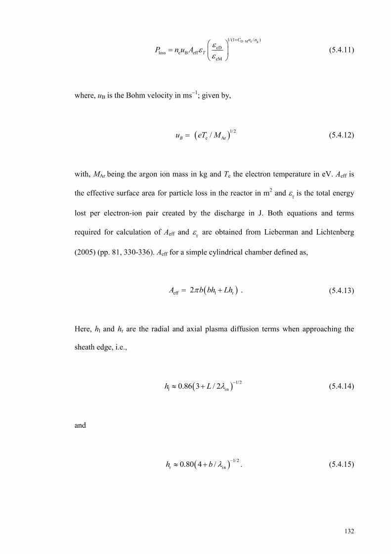
132

D M e g1/(1 / )

cDloss e B eff

cM

C n n

TP n u A

(5.4.11)

where, uB is the Bohm velocity in ms1; given by,

1/2

e Ar /Bu eT M (5.4.12)

with, MAr being the argon ion mass in kg and Te the electron temperature in eV. Aeff is

the effective surface area for particle loss in the reactor in m2 and is the total energy

lost per electron-ion pair created by the discharge in J. Both equations and terms

required for calculation of Aeff and are obtained from Lieberman and Lichtenberg

(2005) (pp. 81, 330-336). Aeff for a simple cylindrical chamber defined as,

eff l r 2 .A b bh Lh (5.4.13)

Here, hl and hr are the radial and axial plasma diffusion terms when approaching the

sheath edge, i.e.,

1/2

l in0.86 3 / 2h L

(5.4.14)

and

1/2

r in0.80 4 / .h b

(5.4.15)

133

L, b and in are the effective chamber height in m, chamber radius in m and ion-neutral

mean free path (given by Chapter 3, Section 3.1.2, Eq. (3.1.4)) in m, respectively.

(calculated in terms of eV) is defined the sum of the collisional energy loss per

ion-electron pair, c, the mean kinetic energy lost per ion,i and the mean kinetic

energy lost per electron, e, i.e.,

T c i e . (eV) (5.4.16)

For argon plasma, the kinetic energy lost per ion and per electron is approximated by, i

≈ 5.2Te and e ≈ 2Te, respectively. The collisional energy loss per ion-electron pair, c,

itself comprises of the total collisional losses due to ionization, excitation and elastic

scattering of electrons with neutrals. It is expressed as,

ex eliz ex e

i

ec

Arz iz

= .3 K K TmMK K

(5.4.17)

Here, iz (eV) is the argon ionization threshold energy and ex (12.14 eV) is

the argon excitation threshold energy. Kiz, Kex and Kel are the argon ionization,

excitation and elastic scattering rate constants (m3s-1) given respectively by,

14 0.59iz e e2.34 10 exp( 17.44 ) ,K T T (5.4.18)

14 0.33ex e e2.48 10 exp( 12.78 ) ,K T T (5.4.19)

134

and

14 1.609 2 3el e e e2.336 10 exp(0.0618ln( ) 0.1171ln( ) ) .K T T T (5.4.20)

respectively. The term (cD/cM)1/(1 + CD-M ne/ng) in Eq. (5.4.11) accounts for the non-linear

effect of transition in electron energy distribution function (EEDF) from Druyvesteyn to

Maxwellian when approaching higher electron densities. The exponential factor CD-M,

adjusts for the experimental discrepancy (due to random and systematic errors) of the

transition point between Druyvesteyn and Maxwellian EEDFs; which is concurrent with

the transition of the discharge from E mode to H mode (Cunge, et al., 1999). ng is the

neutral gas density and is determined from Eq. (5.2.15). cD/cM is the ratio of the

Druyvesteyn and Maxwellian electron-electron collision energy loss factors which is

approximated as,

cD

cM e

9.731.27 .T

(5.4.21)

A MATLAB code for solving the power balance model can be found in Appendix D.

135

CHAPTER 6: RESULTS AND DISCUSSION - SIMULATION

6.0. Predictive Simulation of the Discharge Magnetic Fields

The absolute magnitudes of the axial, |Bz| and radial, |Br| magnetic fields at 0.032 m

distance above the dielectric plate for 0.03, 0.07 and 0.2 mbar argon pressure were

simulated using the numerical H mode model detailed in Chapter 5, Section 5.2. Initial

values for the model were calculated from the analytical H mode model derived in

Chapter 5, Section 5.1. The required spatially resolved electron density, ne (r, z) and

electron temperature, Te (r, z) were empirically fitted. The spatially resolved neutral gas

temperature Tn (r, z), on the other hand, was heuristically fitted in simulation to give the

closest agreement with measured fields at 0.032 m distance above the dielectric plate

and at 180 W r. f. power. For comparison, the magnetic fields were also simulated using

two spatially averaged neutral gas temperatures, Tn,ave; one set at room temperature (300

K) and the other from AOES measurement.1

6.0.1. Empirical Fitting of the Spatially Resolved Electron Density, ne (r, z) and

Spatially Resolved Electron Temperature, Te (r, z)

The spatially resolved electron density, ne (r, z) and the spatially resolved electron

temperature, Te (r, z) required for Eqs. (5.2.10-5.2.13) and Eqs. (5.2.15-5.2.19) were

empirically fitted from the measured Maxwellian values at 0.032, 0.060 and 0.114 m

axial distance above the dielectric plate and at 0.03, 0.07 and 0.2 mbar argon pressure

(Chapter 4, Figures 4.1a, 4.2a and 4.3a) using the following modified Gaussian

distributions:

1 Results in this section comprises of edited and revised material that has been published in Jayapalan and Chin (2014). The thesis author is the primary author and investigator for the paper.

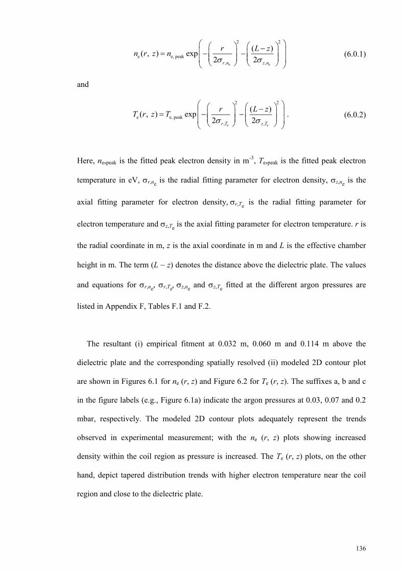
136

e e

e e, peak, ,

2 2( )( , ) exp

2 2

r n z n

r L zn r z n

(6.0.1)

and

e e

e e, pe

2

k, ,

2

a( )( , ) e xp

2 2.

r T z T

r L zT r z T

(6.0.2)

Here, ne,peak is the fitted peak electron density in m-3, Te,peak is the fitted peak electron

temperature in eV, r,ne is the radial fitting parameter for electron density, z,ne is the

axial fitting parameter for electron density,r,Te is the radial fitting parameter for

electron temperature and z,Te is the axial fitting parameter for electron temperature. r is

the radial coordinate in m, z is the axial coordinate in m and L is the effective chamber

height in m. The term (L z) denotes the distance above the dielectric plate. The values

and equations for r,ne, r,Tez,ne and z,Te fitted at the different argon pressures are

listed in Appendix F, Tables F.1 and F.2.

The resultant (i) empirical fitment at 0.032 m, 0.060 m and 0.114 m above the

dielectric plate and the corresponding spatially resolved (ii) modeled 2D contour plot

are shown in Figures 6.1 for ne (r, z) and Figure 6.2 for Te (r, z). The suffixes a, b and c

in the figure labels (e.g., Figure 6.1a) indicate the argon pressures at 0.03, 0.07 and 0.2

mbar, respectively. The modeled 2D contour plots adequately represent the trends

observed in experimental measurement; with the ne (r, z) plots showing increased

density within the coil region as pressure is increased. The Te (r, z) plots, on the other

hand, depict tapered distribution trends with higher electron temperature near the coil

region and close to the dielectric plate.

137

(i)

(ii)

Figure 6.1a: Empirically fitted 2D Gaussian based distribution of electron density ne (r, z) used for the magnetic field simulation at 0.03 mbar argon pressure and 180 W r. f. power. (i) Fitment with measured values at 0.032 m, 0.060 m and 0.114 m distance above the dielectric plate. (ii) Modeled 2D contour plot (labels in m-3).

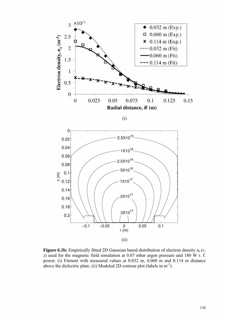
138

(i)

(ii)

Figure 6.1b: Empirically fitted 2D Gaussian based distribution of electron density ne (r, z) used for the magnetic field simulation at 0.07 mbar argon pressure and 180 W r. f. power. (i) Fitment with measured values at 0.032 m, 0.060 m and 0.114 m distance above the dielectric plate. (ii) Modeled 2D contour plot (labels in m-3).

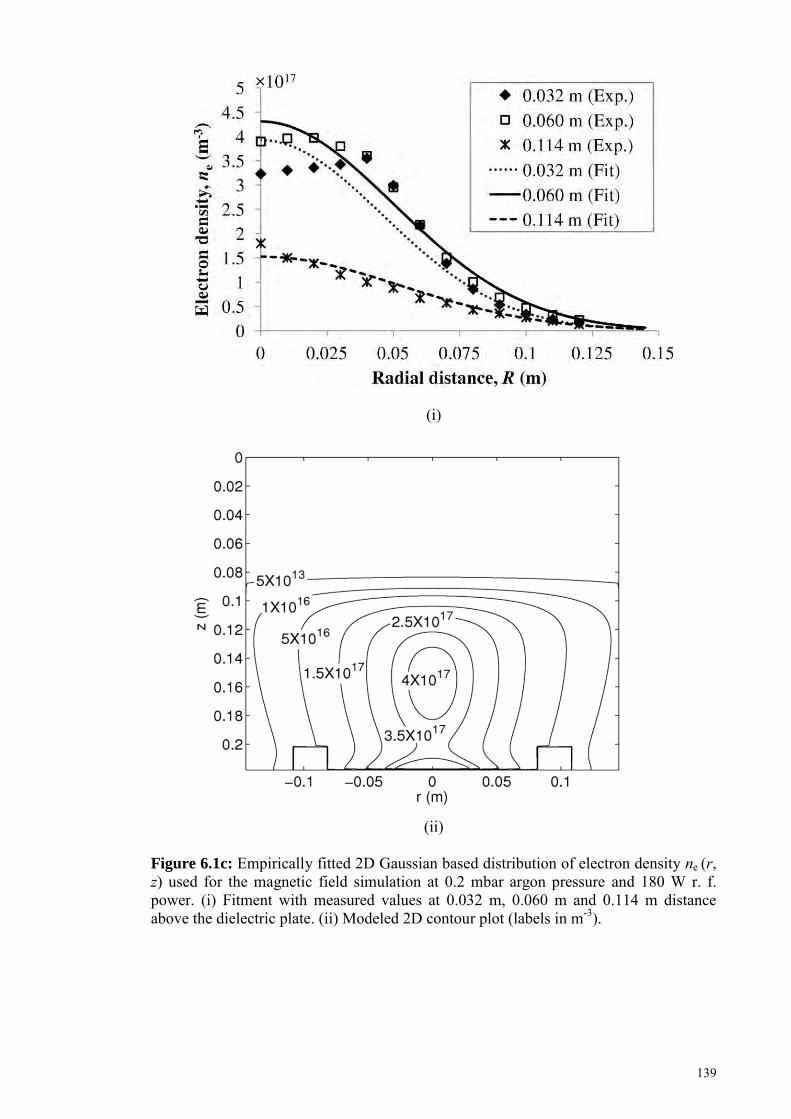
139

(i)

(ii)

Figure 6.1c: Empirically fitted 2D Gaussian based distribution of electron density ne (r, z) used for the magnetic field simulation at 0.2 mbar argon pressure and 180 W r. f. power. (i) Fitment with measured values at 0.032 m, 0.060 m and 0.114 m distance above the dielectric plate. (ii) Modeled 2D contour plot (labels in m-3).

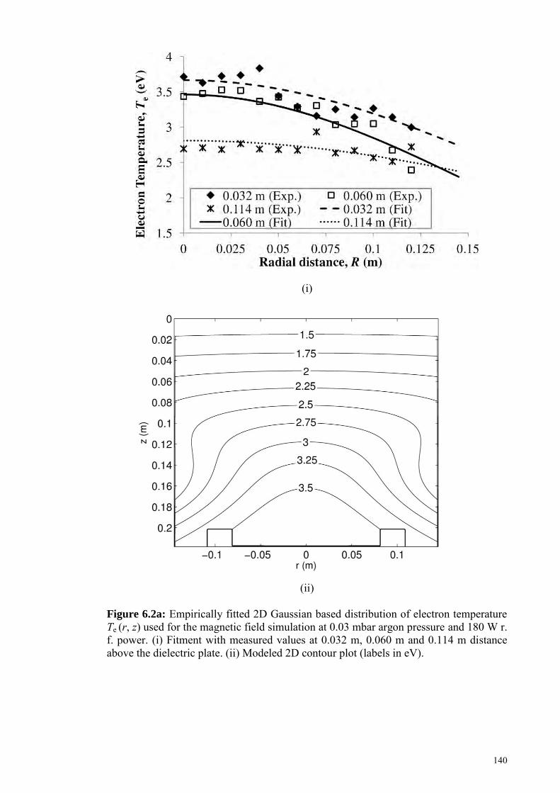
140

(i)

(ii)

Figure 6.2a: Empirically fitted 2D Gaussian based distribution of electron temperature Te (r, z) used for the magnetic field simulation at 0.03 mbar argon pressure and 180 W r. f. power. (i) Fitment with measured values at 0.032 m, 0.060 m and 0.114 m distance above the dielectric plate. (ii) Modeled 2D contour plot (labels in eV).

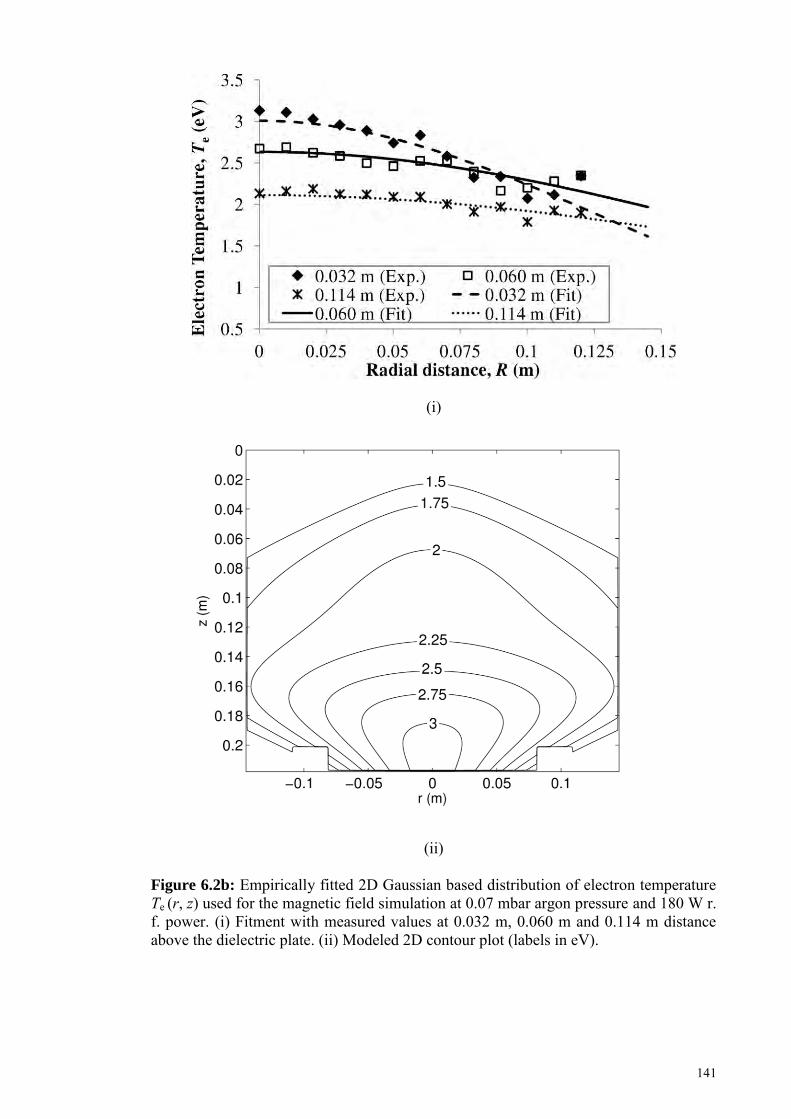
141

(i)

(ii)

Figure 6.2b: Empirically fitted 2D Gaussian based distribution of electron temperature Te (r, z) used for the magnetic field simulation at 0.07 mbar argon pressure and 180 W r. f. power. (i) Fitment with measured values at 0.032 m, 0.060 m and 0.114 m distance above the dielectric plate. (ii) Modeled 2D contour plot (labels in eV).

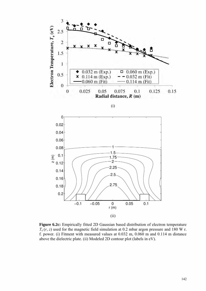
142

(i)

(ii)

Figure 6.2c: Empirically fitted 2D Gaussian based distribution of electron temperature Te (r, z) used for the magnetic field simulation at 0.2 mbar argon pressure and 180 W r. f. power. (i) Fitment with measured values at 0.032 m, 0.060 m and 0.114 m distance above the dielectric plate. (ii) Modeled 2D contour plot (labels in eV).

143

6.0.2. Heuristic fitting of the Spatially Resolved Neutral Gas Temperature, Tn (r, z)

Using the similar modified Gaussian function in Section 6.0.1, the spatially resolved

neutral gas temperature, Tn (r, z) was heuristically fitted in simulation to values that give

the closest agreement to the measured magnetic fields at 0.032 m axial distance above

the dielectric plate and 180 W r. f. power. The function can be written as,

n

n n, peak,

2

,

2( )( , ) ex p

2 2,

nr T z T

r L zT r z T

(6.0.3)

where, Tn,peak is the fitted peak neutral gas temperature in K, r,Tn is the radial fitting

parameter for neutral gas temperature and z,Tn is the axial fitting parameter for neutral

gas temperature. Values for r,Tn and z,Tn for different argon pressures simulated are

given in Appendix F, Table F.3.

The 2D contour plots of the heuristic Tn (r, z) fitments that gave the best agreement

with measured values for 0.03, 0.07 and 0.2 mbar argon pressures are shown in Figures

6.3 (a), 6.3 (b) and 6.3 (c), respectively. The fitted peak temperatures, Tn,peak were in the

range of 1800-2300 K; values which may be considered high if compared with other

reported works (Table 6.1). The distribution of Tn (r, z) was observed to peak at the

center of the chamber above the dielectric plate; tapering off gradually at the axial

direction and rapidly towards the edge of the coil at all pressures. Heating of the

neutrals (i.e., Tn (r, z) > 300 K) for all pressures was mostly confined within the coil

region, with increase in distribution temperature as argon pressure was increased.

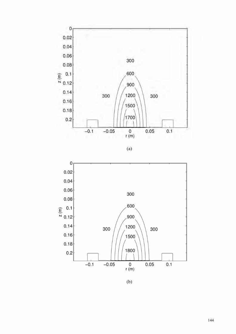
144

(a)

(b)

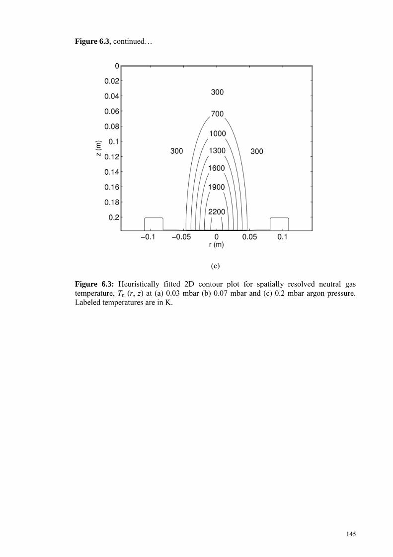
145

Figure 6.3, continued…

(c)

Figure 6.3: Heuristically fitted 2D contour plot for spatially resolved neutral gas temperature, Tn (r, z) at (a) 0.03 mbar (b) 0.07 mbar and (c) 0.2 mbar argon pressure. Labeled temperatures are in K.

146

Table 6.1: Comparison of parameters of present setup with other reported works of similar ICPs.

Parameters Present Setup

Ostrikov et al.

(2002)

Hebner (1996)

Sadeghi et al,

(1997)

Shimada et al.

(2007, 2008)

Li et al. (2011)

Pressure P (mbar) 0.07 0.04 0.04 0.05 0.01 0.07

ne (m3) 1017 1017 1017 - 1017 1017

Te (eV) 2.0-3.1 2.0-2.1 - - 2.5 -

Measured Tn (K) 630 543 1100 650 - 1200 Radial range of Tn

(K) 300-1900 - - - 600-900 -

Coil radius, a (m) *helical coil 0.045 0.160 0.055 *0.050 *0.055 0.104

Chamber inner radius, b (m) 0.145 0.160 0.065 0.075 0.175 0.104

Axial distance from dielectric plate,

(L z) (m) 0.032 0.060 0.016 - 0.160 -

Power (W) 180 612.4 200 400 2000 200

Surface power density, r. f. power /

coil area (Wm2) 2.82 0.76 2.10 - - 0.59

r. f. Frequency (MHz) 13.56 0.46 13.56 13.56 13.56 13.56

These observations can be justified by the following points:

i. The surface power density (2.82 Wm-2) is higher for the present setup as

compared to the other works due to smaller coil dimensions, i.e., coil radius ~

0.045 m whereas, chamber radius ~ 0.145 m. This translates to more

concentrated heating of the plasma particles by the source power over a smaller

chamber volume, which subsequently results in increased localized

thermalization of the neutral particles. Other comparative systems have larger

coils (at equal diameters with the chamber) which would attribute to a lower

surface power density at the same power. Thus, the power deposited by the

147

inductive coils into these systems would be distributed in a wider area and the

consequential effect of neutral gas heating would be less.

ii. The trend of the spatial distributions obtained (i.e., in which the neutral gas is the

hottest at the center above the dielectric plate and tapers off rapidly at the axial

direction and towards the edge of the coil) is valid and has been reported in

measurement by Shimada, Tynan and Cattolica, 2007.

iii. The increase in neutral gas heating with argon pressure is attributed to increased

r. f. power coupling from the source coil to the plasma particles with pressure.

To demonstrate this, it would be convenient to first tabulate the relevant power

balance parameters; derived from the theoretical equations in Chapter 5,

Sections 5.2.1 and 5.4. The effective collision frequency, veff and the total

absorbed electron power, Pabs were calculated for the fitted argon pressures, P

using the measured peak coil current, Ip, the measured average electron density,

ne,coil and electron temperature, Te,coil across the coil radius (for 180 W input r.f.

power) and the set peak neutral gas temperature, Tn,peak (Table 6.2).

Table 6.2: Calculated values for effective collision frequency, veff and total absorbed electron power, Pabs with measured average coil electron density, ne,coil, average coil electron temperature, Te,coil and peak coil current, Ip (for 180 W input r.f. power) and set peak neutral gas temperature, Tn,peak at 0.03, 0.07 and 0.2 mbar argon pressure.

Argon Pressure, P (mbar)

ne, coil (m-3) Te, coil (eV) Ip (A) Tn,peak (K) veff (s-1) Pabs (W)

0.03 6.95 × 1016 3.68 14.8 1800 5.46 × 107 79.9

0.07 2.15 × 1017 2.97 14.2 1900 8.35 × 107 118.2

0.2 3.31 × 1017 2.78 13.8 2300 1.29 × 108 145.0

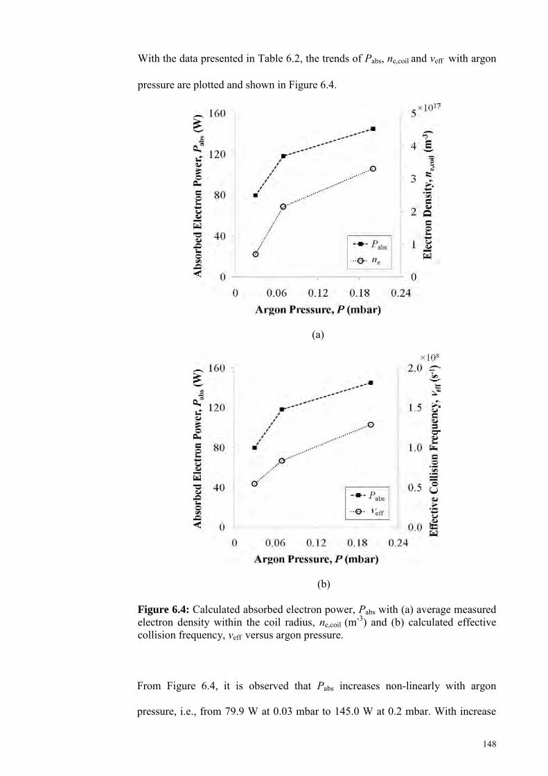
148

With the data presented in Table 6.2, the trends of Pabs, ne,coil and veffwith argon

pressure are plotted and shown in Figure 6.4.

(a)

(b)

Figure 6.4: Calculated absorbed electron power, Pabs with (a) average measured electron density within the coil radius, ne,coil (m-3) and (b) calculated effective collision frequency, veff versus argon pressure.

From Figure 6.4, it is observed that Pabs increases non-linearly with argon

pressure, i.e., from 79.9 W at 0.03 mbar to 145.0 W at 0.2 mbar. With increase

149

in Pabs, ne,coil also becomes higher (Figure 6.4 (a)). Higher ne,coil at higher

pressures would mean that there is higher number of ions available within the

coil region for heating by the oscillating r. f. fields (Shimada, Tynan & Cattolica,

2008). These accelerated ions are highly energized and can reach very high

temperatures (Hebner, 1996). Since effective collision frequency also increases

with pressure (Figure 6.4 (b)), more of these highly energized ions would be

converted into thermalized neutrals via de-excitation with electrons and elastic

or charge transfer collisions with other neutrals (Lieberman & Lichtenberg,

2005). Hence, the increase in formation thermalized neutrals would contribute to

the increase in neutral gas heating with pressure; as seen in fitment.

6.0.3. Spatially averaged neutral gas temperatures, Tn,ave

For comparison with simulations using Tn(r, z), the magnetic fields were also

calculated with spatially averaged neutral gas temperature values, Tn,ave. Tn,ave was set at

both room temperature (Tn,ave = 300 K) and measured temperature. The measured values

used for simulation were 380, 630 and 800 K for 0.03, 0.07 and 0.2 mbar argon

pressure, respectively; corresponding to the results at 0.032 m axial distance obtained

from Chapter 4, Section 4.3.1, Figure 4.10.

6.0.4. Comparison of Measured and Simulated Magnetic Fields

Measured axial and radial magnetic fields are compared to simulated values for 0.03,

0.07 and 0.2 mbar argon pressures at 0.032 m above the dielectric plate as shown in

Figures 6.5a, 6.5b and 6.5c. At 180 W r. f. power, the measured peak coil currents, Ip

were 14.4 A for 0.03 mbar, 14.2 A for 0.07 mbar and 13.4 A for 0.2 mbar; values

that were used for simulation.

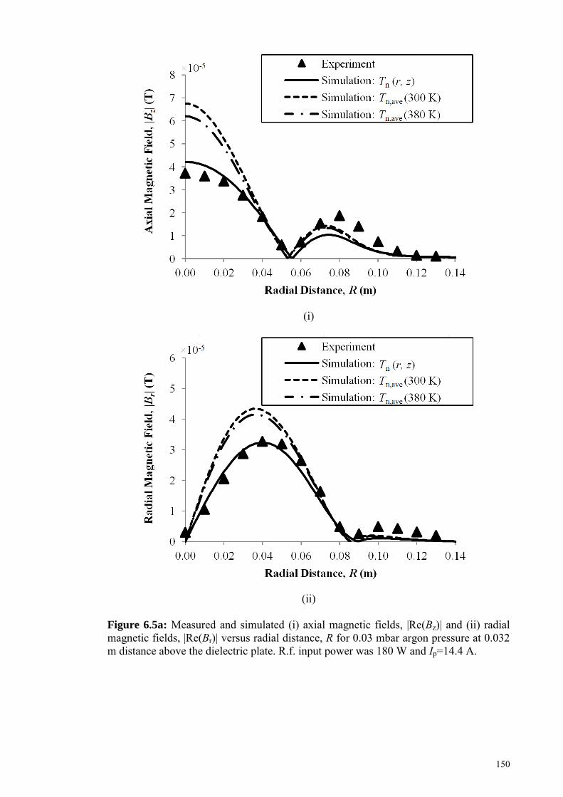
150

(i)

(ii)

Figure 6.5a: Measured and simulated (i) axial magnetic fields, |Re(Bz)| and (ii) radial magnetic fields, |Re(Br)| versus radial distance, R for 0.03 mbar argon pressure at 0.032 m distance above the dielectric plate. R.f. input power was 180 W and Ip=14.4 A.

151

(i)

(ii)

Figure 6.5b: Measured and simulated (i) axial magnetic fields, |Re(Bz)| and (ii) radial magnetic fields, |Re(Br)| versus radial distance, R for 0.07 mbar argon pressure at 0.032 m distance above the dielectric plate. R.f. input power was 180 W and Ip=14.2 A.

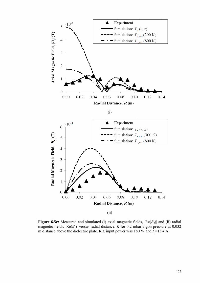
152

(i)

(ii)

Figure 6.5c: Measured and simulated (i) axial magnetic fields, |Re(Bz)| and (ii) radial magnetic fields, |Re(Br)| versus radial distance, R for 0.2 mbar argon pressure at 0.032 m distance above the dielectric plate. R.f. input power was 180 W and Ip=13.4 A.

153

The simulated fields were computed using neutral gas temperature that was spatially

resolved, Tn (r, z) and its spatially averaged values Tn,ave at room and measured

temperature. Suppression of the magnetic fields (especially at the centre axis of the

chamber, i.e., R 0 m) is seen to progressively increase with chamber pressure and is

especially prominent at 0.07 mbar and 0.2 mbar. This suppression trend is only

sufficiently matched by the simulation with the spatially resolved neutral gas

temperature, Tn (r, z) and not the spatially averaged neutral temperatures, Tn,ave.

The mechanism of the suppression of the magnetic fields can be explained as

follows. When the discharge is initiated, inductive coupling would result in ionization of

the argon neutrals to form ion-electron pairs. These ion-electron pairs move freely in the

plasma region and may be thermalized under the influence of the bulk ambipolar

electrostatic field (Shimada, Tynan & Cattolica, 2008). Further thermalization of the

charged particles also occurs via Coulomb collisions and stochastic heating by the

oscillating capacitive sheath (Gudmunsson & Lieberman, 1998). Ions thermalized by

these interactions (reaching temperatures of 1000-4000 K as reported by Hebner, 1996)

will subsequently undergo collisional processes with electrons via de-excitation and

elastic or charge transfer collisions with other neutrals, forming thermalized neutrals

that increase the neutral temperature in the vicinity. These thermalized neutrals, which

at the beginning, are formed mostly at the center of the discharge region would create a

pressure and temperature gradient across the coil radius that would lead to convection of

these particles towards the edge of the coil.

As a result of this convection, a depletion of neutral gas density will start to occur at

the central region of the plasma. As this depletion profile grows, the mean free path of

the plasma particles (including the neutrals) is increased, thus, allowing for more highly

energetic particles to exist (Fruchtman et al., 2005). Heating of these background

154

particles would also generate a localized environment whereby less energy is required to

sustain ion-electron pairs; increasing the utilization of the magnetic fields by the plasma

(Turner & Lieberman, 1999). The depletion of neutrals at the centre of the plasma

region would continue until an equilibrium state is formed between the number of

available neutrals and ionization of new plasma electrons.

At higher pressures, this equilibrium state occurs at higher electron densities due to

the higher number of neutrals, thus, resulting in higher utilization of the incident fields

with increased suppression (Figure 6.5c). Consequently, the increased utilization of the

magnetic fields in the centre reduces the skin depth in the region of effect, i.e., the coil

radius. The comparative effect of neutral gas heating on the magnetic fields can be seen

in Figures 6.5 whereby in the case of 300 K, the simulated fields are much higher than

the experimentally measured values. This suggests that part of the energy coupled into

the plasma particles has been distributed to the neutrals and hence, it is inferred that

neutral gas heating plays an important role in determining the skin depth of the

magnetic fields. Knowledge of the non-uniform distribution of neutral gas temperature

across the chamber radius is also essential for accurate deduction of field suppression

trends.

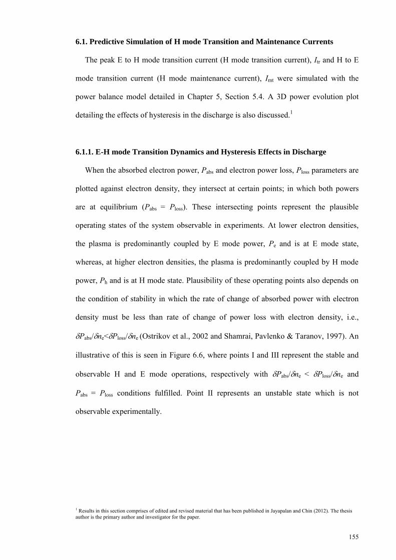
155

6.1. Predictive Simulation of H mode Transition and Maintenance Currents

The peak E to H mode transition current (H mode transition current), Itr and H to E

mode transition current (H mode maintenance current), Imt were simulated with the

power balance model detailed in Chapter 5, Section 5.4. A 3D power evolution plot

detailing the effects of hysteresis in the discharge is also discussed.1

6.1.1. E-H mode Transition Dynamics and Hysteresis Effects in Discharge

When the absorbed electron power, Pabs and electron power loss, Ploss parameters are

plotted against electron density, they intersect at certain points; in which both powers

are at equilibrium (Pabs = Ploss). These intersecting points represent the plausible

operating states of the system observable in experiments. At lower electron densities,

the plasma is predominantly coupled by E mode power, Pe and is at E mode state,

whereas, at higher electron densities, the plasma is predominantly coupled by H mode

power, Ph and is at H mode state. Plausibility of these operating points also depends on

the condition of stability in which the rate of change of absorbed power with electron

density must be less than rate of change of power loss with electron density, i.e.,

Pabs/ne<Ploss/ne (Ostrikov et al., 2002 and Shamrai, Pavlenko & Taranov, 1997). An

illustrative of this is seen in Figure 6.6, where points I and III represent the stable and

observable H and E mode operations, respectively with Pabs/ne < Ploss/ne and

Pabs = Ploss conditions fulfilled. Point II represents an unstable state which is not

observable experimentally.

1 Results in this section comprises of edited and revised material that has been published in Jayapalan and Chin (2012). The thesis author is the primary author and investigator for the paper.

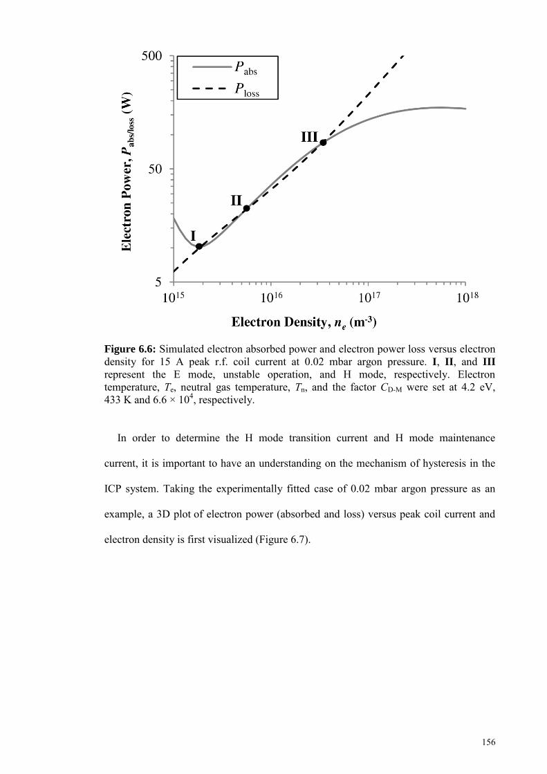
156

Figure 6.6: Simulated electron absorbed power and electron power loss versus electron density for 15 A peak r.f. coil current at 0.02 mbar argon pressure. I, II, and III represent the E mode, unstable operation, and H mode, respectively. Electron temperature, Te, neutral gas temperature, Tn, and the factor CD-M were set at 4.2 eV, 433 K and 6.6 × 104, respectively.

In order to determine the H mode transition current and H mode maintenance

current, it is important to have an understanding on the mechanism of hysteresis in the

ICP system. Taking the experimentally fitted case of 0.02 mbar argon pressure as an

example, a 3D plot of electron power (absorbed and loss) versus peak coil current and

electron density is first visualized (Figure 6.7).

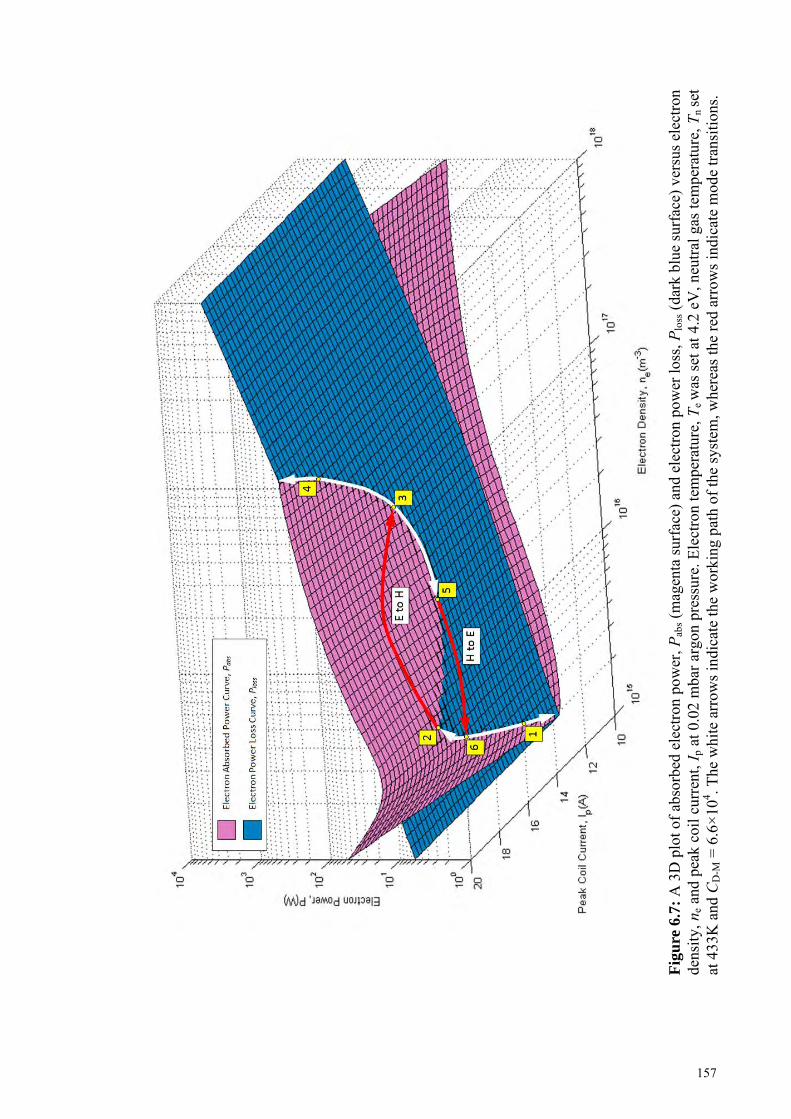
157

Fig

ure

6.7

: A

3D

plo

t of a

bsor

bed

elec

tron

pow

er, P

abs (

mag

enta

surf

ace)

and

ele

ctro

n po

wer

loss

, Plo

ss (d

ark

blue

surf

ace)

ver

sus e

lect

ron

dens

ity, n

e and

pea

k co

il cu

rren

t, I p

at 0

.02

mba

r arg

on p

ress

ure.

Ele

ctro

n te

mpe

ratu

re, T

e w

as se

t at 4

.2 e

V, n

eutra

l gas

tem

pera

ture

, Tn

set

at 4

33K

and

CD

-M =

6.6

×104 . T

he w

hite

arr

ows i

ndic

ate

the

wor

king

pat

h of

the

syst

em, w

here

as th

e re

d ar

row

s ind

icat

e m

ode

trans

ition

s.

158

The magenta (lighter) surface of the 3D plot represents the evolution of absorbed

electron power, Pabs whereas dark blue (darker) surface represents the evolution of

electron power loss, Ploss. As aforementioned, the intersections between the two surfaces

represent the working path of the system. In a typical experiment, the input coil current

starts at zero. As the input coil current (or r.f. power) is increased, the operating point of

the system moves to point 1 (Figures 6.7 and 6.8).

Figure 6.8: The simulated absorbed electron power (solid line) and power loss (dashed line) curves depicting (a) the current at which either E mode (13 A) or H mode operation (18 A) alone occurs.

At this point, the low density E mode plasma is observed (E mode was ignited before

point 1 at input coil current of 5.2 ± 0.2 A). A further increase in current would shift the

operating point of the system to point 2. Point 2 is the threshold at which any further

increase in coil current would trigger a transition from E to H mode, marking the H

mode transition current (Figures 6.7 and 6.9).

159

(b)

Figure 6.9: The simulated absorbed electron power (solid line) and power loss (dashed line) curves depicting the threshold currents for E to H (16.41 A) and H to E (14.19 A) mode transitions. From point 2, the system jumps to point 3 which is in H mode. Point 3 is determined

experimentally and is affected by the sensitivity and accuracy of the impedance

matching circuit (El-Fayoumi, Jones & Turner, 1998, Cunge, et al., 1999 and Turner &

Lieberman, 1999). Increase in coil current at point 3 would bring system operation to

point 4 (Figures 6.7 and 6.8) which is higher density plasma in H mode. When coil

current is decreased from point 4, the system follows the working H mode path until

point 5. Point 5 is the threshold at which a further decrease would trigger a transition to

E mode (Figures 6.7 and 6.9). This threshold point is measured as the minimum or

maintenance current for H mode plasma. The disparity between transition and

maintenance currents (as observed in the plot) denotes the effect of hysteresis in the

working path of the system. From point 5, a decrease in coil current shifts the system

operation to point 6 which is in E mode.

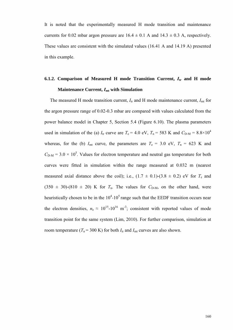
160

It is noted that the experimentally measured H mode transition and maintenance

currents for 0.02 mbar argon pressure are 16.4 ± 0.1 A and 14.3 ± 0.3 A, respectively.

These values are consistent with the simulated values (16.41 A and 14.19 A) presented

in this example.

6.1.2. Comparison of Measured H mode Transition Current, Itr and H mode

Maintenance Current, Imt with Simulation

The measured H mode transition current, Itr and H mode maintenance current, Imt for

the argon pressure range of 0.02-0.3 mbar are compared with values calculated from the

power balance model in Chapter 5, Section 5.4 (Figure 6.10). The plasma parameters

used in simulation of the (a) Itr curve are Te = 4.0 eV, Tn = 583 K and CD-M = 8.8×104

whereas, for the (b) Imt curve, the parameters are Te = 3.0 eV, Tn = 623 K and

CD-M = 3.0 × 105. Values for electron temperature and neutral gas temperature for both

curves were fitted in simulation within the range measured at 0.032 m (nearest

measured axial distance above the coil); i.e., (1.7 ± 0.1)-(3.8 ± 0.2) eV for Te and

(350 ± 30)-(810 ± 20) K for Tn. The values for CD-M, on the other hand, were

heuristically chosen to be in the 104-105 range such that the EEDF transition occurs near

the electron densities, ne ≈ 1015-1016 m-3; consistent with reported values of mode

transition point for the same system (Lim, 2010). For further comparison, simulation at

room temperature (Tn = 300 K) for both Itr and Imt curves are also shown.

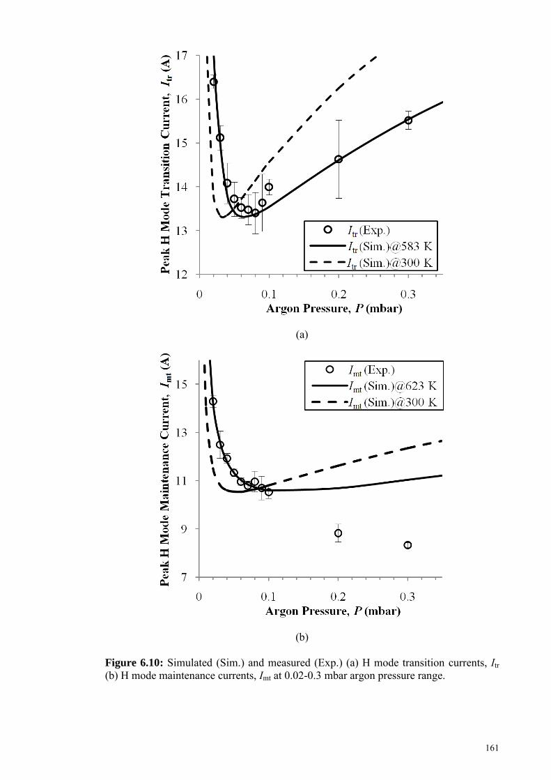
161

(a)

(b)

Figure 6.10: Simulated (Sim.) and measured (Exp.) (a) H mode transition currents, Itr (b) H mode maintenance currents, Imt at 0.02-0.3 mbar argon pressure range.

162

In Figure 6.10 (a), it is observed that the simulated Itr curve is well matched to the

measured values when neutral gas heating is considered. At room temperature, however,

the Itr curve does not match. Measured Itr values are higher than simulated Itr values at

room temperature at lower filling pressures of <0.06 mbar; whereas, at higher filling

pressures of >0.06 mbar, the measured Itr, values are lower. At lower filling pressure,

thermalization of the neutrals diffuses the particles in the plasma in accordance to ideal

gas law (O' Connell et al., 2008, Shimada, Tynan & Cattolica, 2008). Since, the plasma

is diffused, higher input current is required to generate sufficient plasma ionization and

reach threshold electron density to attain H mode (Fruchtman, 2008). At higher filling

pressures, the neutral gas density of the plasma has become high enough such that

thermalization of the neutral particles increases the power transfer efficiency by

assisting plasma collisional processes (Lieberman & Lichtenberg, 2005 and Suzuki et

al., 1998). This reduces the input Itr required to sustain H mode.

In Figure 6.10 (b), the simulated Imt curve with neutral gas heating is well matched to

the measured values at the range of and 0.02-0.1 mbar. Discrepancy between the

measured Imt and simulated Imt curves at room temperature can also be explained in the

same way as the Itr curve; with thermalization of the neutrals in experiment diffusing the

plasma at lower filling pressures (<0.09 mbar) and assisting in plasma collision

processes at higher filling pressures (>0.09 mbar). The higher pressure region at which

diffusion of the particles influence Imt (~0.09 mbar) as compared to Itr (~0.06 mbar) is

due to the lower plasma density at which the H to E mode transition occurs.

The increasing deviation at higher pressures of 0.2-0.3 mbar between the simulated

and experimental Imt curves is suspected to be due to the non-linear effects of multistep

ionization which is yet to be included in the simulation. At higher pressures, complex

163

ionization processes occurring from intermediary or metastable excitation states become

more significant such that the total energy required to sustain the ion-electron pairs

created in the discharge is further reduced, i.e., lower electron power loss (Turner &

Lieberman, 1999). This effect, in part, explains the ability of the H mode discharge in

experiment to be maintained at a much lower current than the values obtained by

simulation.

164

CHAPTER 7: SUMMARY AND CONCLUSION

7.0. Overview

In this study, a 13.56 MHz, 6 turn planar coil, argon inductively coupled plasma

(ICP) was characterized with a combination of experimental diagnostic techniques and

predictive simulation; from which the effects of neutral gas heating was observed.

Summary of the results obtained are given in following sections along with key findings

and suggestions for future work.

7.1. Experimental Characterization

Experimental characterization was done using several diagnostic probes; with each

measuring different properties of the plasma. Electrical properties such as the radially

resolved electron density, ne, the radially resolved electron temperature, Te and the

electron energy distribution function, EEDF at the chamber center (R = 0) were

measured using a r.f. compensated Langmuir probe. The spatially resolved absolute

axial magnetic fields, |Bz| and absolute radial magnetic fields, |Br| were measured using

two electrostatically compensated magnetic probes at the respective orientations. The

peak H mode transition current, Itr and peak H mode maintenance peak current, Imt were

measured using a current probe attached to the source coil. The neutral gas temperature,

Tn of the discharge was measured via the AOES technique.

7.1.1. Measurement of Electron Density, ne and Electron Temperature, Te and

Electron Energy Distribution Function (EEDF)

The radially resolved electron density, ne and electron temperature, Te of the

discharge were measured at 0.03, 0.07 and 0.2 mbar argon pressure for 0.032 m, 0.060

and 0.114 axial distances above the dielectric plate and calculated using Maxwellian and

165

EEDF methods. R.f. power was set at 180 W. Higher values of ne and lower values of Te

were obtained using the Maxwellian method in comparison to the EEDF method. With

increase in argon pressure for all measured radial positions, ne increases and Te decreases.

The range of electron densities obtained were (0.065 ± 0.004)-(4.0 ± 0.6) × 1017 m-3 for the

Maxwellian method and (0.052 ± 0.004)-(3.5 ± 0.5) × 1017 m-3 for the EEDF method.

The range of values measured for Te, on the other hand, were (1.38 ± 0.08)-(3.8 ± 0.2) eV

using the Maxwellian method and (1.78 ± 0.05)-(4.8 ± 0.3) eV using the EEDF method.

Several important observations were made:

i. As argon pressure was increased, the discharge becomes increasingly denser

within the coil region (R < 0.05 m). This was attributed to the increase in plasma

collision frequency with argon particles, producing more ionizing collisions in

the region where the r.f. source field was the strongest. This was further validated

by the simulation results for the total absorbed electron power, Pabs (Chapter 6,

Section 6.0.2, Table 6.2); whereby, for measured parameters at 180 W input r.f.

power, Pabs increases with argon pressure.

ii. ne at 0.2 mbar did not decrease (as expected) with reduced proximity from the

source r.f. field. Instead, ne within the coil region was highest at 0.060 m axial

distance above the dielectric plate. The observed displacement between power

deposition of the source r.f. field and region of maximum ne was likely to be from

enhanced plasma transport due to neutral gas heating; with particles forming a

steady state flux due to temperature gradient and travelling away from the source

coil and towards the chamber walls.

166

iii. The radial distribution of ne at 0.2 mbar argon pressure for 0.032 m axial distance

above the dielectric plate (close to the source) was higher at the edge of the coil

region and did not follow the other distribution trends which peaked at R = 0.

This was also attributed to enhanced plasma transport due to neutral gas heating;

as plasma particles were pushed away from the discharge center towards the edge

of the coil region due to temperature gradient.

iv. Te distribution for 0.2 mbar argon pressure showed increased number of higher

energy electrons near the coil region. This supports the notion of neutral gas

heating, which would cause the plasma collision frequency in the vicinity of

effect to be comparatively less than the plasma collision frequency of the

surrounding area and thus, allow for higher accumulation of electron energy via

increased free mean path.

As with ne and Te, the EEDFs at the chamber center (R 0) at 0.03, 0.07 and 0.2

mbar argon pressure for 0.032 m, 0.060 and 0.114 axial distances above the dielectric

plate were also calculated and parametrically fitted (as the electron energy probability

function or EEPF) with defined Maxwellian or Druyvestyen functions (Table 7.1).

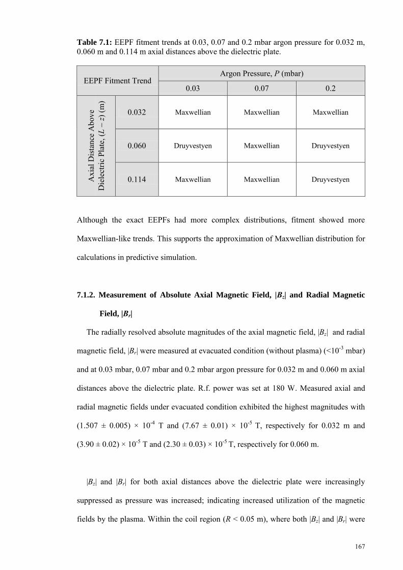
167

Table 7.1: EEPF fitment trends at 0.03, 0.07 and 0.2 mbar argon pressure for 0.032 m, 0.060 m and 0.114 m axial distances above the dielectric plate.

EEPF Fitment Trend Argon Pressure, P (mbar)

0.03 0.07 0.2 A

xial

Dis

tanc

e A

bove

D

iele

ctric

Pla

te, (

L z)

(m)

0.032 Maxwellian Maxwellian Maxwellian

0.060 Druyvestyen Maxwellian Druyvestyen

0.114 Maxwellian Maxwellian Druyvestyen

Although the exact EEPFs had more complex distributions, fitment showed more

Maxwellian-like trends. This supports the approximation of Maxwellian distribution for

calculations in predictive simulation.

7.1.2. Measurement of Absolute Axial Magnetic Field, |Bz| and Radial Magnetic

Field, |Br|

The radially resolved absolute magnitudes of the axial magnetic field, |Bz| and radial

magnetic field, |Br| were measured at evacuated condition (without plasma) (<10-3 mbar)

and at 0.03 mbar, 0.07 mbar and 0.2 mbar argon pressure for 0.032 m and 0.060 m axial

distances above the dielectric plate. R.f. power was set at 180 W. Measured axial and

radial magnetic fields under evacuated condition exhibited the highest magnitudes with

(1.507 ± 0.005) × 10-4 T and (7.67 ± 0.01) × 10-5 T, respectively for 0.032 m and

(3.90 ± 0.02) × 10-5 T and (2.30 ± 0.03) × 10-5 T, respectively for 0.060 m.

|Bz| and |Br| for both axial distances above the dielectric plate were increasingly

suppressed as pressure was increased; indicating increased utilization of the magnetic

fields by the plasma. Within the coil region (R < 0.05 m), where both |Bz| and |Br| were

168

most utilized, a trough was formed with increase in pressure. This observation was

consistent with the distribution trends seen in ne.

7.1.3. Measurement of Peak H Mode Transition, Itr and H Mode Maintenance

Currents, Imt

H mode transition current (E to H mode transition current), Itr and H mode

maintenance current (H to E mode transition current), Imt was measured for the argon

pressure range of 0.02-0.3 mbar. At 0.02 mbar, Itr = (16.4 ± 0.2) A was required to

initiate a transition from E mode to H mode. As pressure was increased, Itr decreased to

a minimum value of (13.5 ± 0.5) A at 0.08 mbar before subsequently increasing to

(15.5 ± 0.2) A at 0.3 mbar. This is attributed to the power coupling of source fields

which has been shown to be most efficient when eff≈ 1; found at the simulated

pressures of 0.07-0.08 mbar. For Imt at 0.02 mbar, (14.3 ± 0.2) A was required to

maintain the discharge. As pressure was increased, Imt decreases consistently to (8.3 ±

0.1) A at 0.3 mbar. The effect of hysteresis in the working path of the system with

pressure was seen from the increasing deviation between Itr and Imt values. The lower Imt

requirement at higher pressures was explained by the following points:

i. At higher discharge pressures (with higher electron densities), multi-step

ionization becomes the primary process of conversion of absorbed excited state

energy over radiative de-excitation processes. Thus, more energy from the

excitation collisions that occur contributes toward the ionization of particles, i.e.,

lower Imt.

ii. Increase in plasma collision frequency with pressure increases the number of

ionizing collisions, allowing for lower Imt.

169

iii. From results in AOES measurement, the neutral gas temperature of the discharge

was also seen to increase with pressure. With the background particles having

higher kinetic energy, they were more readily ionized in collisional processes.

This would result in lower Imt with pressure.

7.1.4. Measurement of Neutral Gas Temperature, Tn

The neutral gas temperature, Tn was measured at 0.03, 0.05, 0.07, 0.1 and 0.2 mbar

Ar/N2 pressures for increasing and decreasing r.f. power steps at 0.032 m and 0.060 m

axial distance above the dielectric plate. Changes in r.f. power and distances above the

dielectric plate showed little variation in Tn. Significant increase in Tn, however, was

observed when pressure was increased. These trends were explained by the following

points:

i. As Ar/N2 pressure is increased at a fixed input r.f. power, more energy is coupled

into the plasma; thus, increasing electron density and ion density. With more

charged and neutral particles within the same volume, the collision frequency of

the plasma particles increases. Transfer of kinetic energy from charged particles

to neutral particles is increased via charge transfer collision of energetic ions with

neutrals and de-excitation collision of ions by electrons; raising the number of

thermalized neutrals within the plasma and increasing Tn.

ii. With collisional processes limited by collision frequency, variation of r.f. power

does not significantly affect Tn; owing to the limited energy transfer from

charged particles to the neutrals.

iii. The convection of thermalized neutrals would mean that the particles would also

be distributed to regions further from the source. Thus, at the measured axial

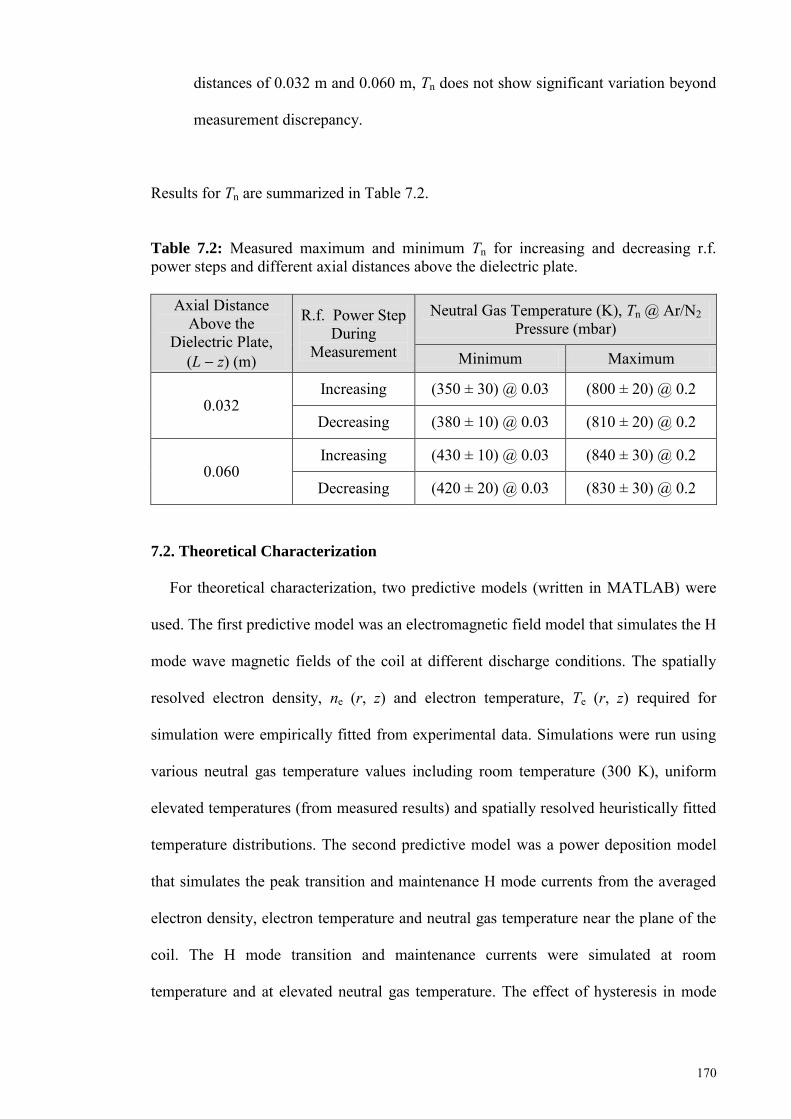
170

distances of 0.032 m and 0.060 m, Tn does not show significant variation beyond

measurement discrepancy.

Results for Tn are summarized in Table 7.2.

Table 7.2: Measured maximum and minimum Tn for increasing and decreasing r.f. power steps and different axial distances above the dielectric plate.

Axial Distance Above the

Dielectric Plate, (L z) (m)

R.f. Power Step During

Measurement

Neutral Gas Temperature (K), Tn @ Ar/N2 Pressure (mbar)

Minimum Maximum

0.032 Increasing (350 ± 30) @ 0.03 (800 ± 20) @ 0.2

Decreasing (380 ± 10) @ 0.03 (810 ± 20) @ 0.2

0.060 Increasing (430 ± 10) @ 0.03 (840 ± 30) @ 0.2

Decreasing (420 ± 20) @ 0.03 (830 ± 30) @ 0.2

7.2. Theoretical Characterization

For theoretical characterization, two predictive models (written in MATLAB) were

used. The first predictive model was an electromagnetic field model that simulates the H

mode wave magnetic fields of the coil at different discharge conditions. The spatially

resolved electron density, ne (r, z) and electron temperature, Te (r, z) required for

simulation were empirically fitted from experimental data. Simulations were run using

various neutral gas temperature values including room temperature (300 K), uniform

elevated temperatures (from measured results) and spatially resolved heuristically fitted

temperature distributions. The second predictive model was a power deposition model

that simulates the peak transition and maintenance H mode currents from the averaged

electron density, electron temperature and neutral gas temperature near the plane of the

coil. The H mode transition and maintenance currents were simulated at room

temperature and at elevated neutral gas temperature. The effect of hysteresis in mode

171

transition of the discharge was also demonstrated using an experimentally fitted 3D

power evolution plot.

7.2.1. Predictive Simulation of the Discharge Magnetic Fields

The axial and radial magnetic field distributions in a 13.56 MHz 6-turn planar coil

ICP reactor were predictively simulated for 0.03, 0.07, and 0.2 mbar argon pressures

with the consideration of the effect of neutral gas heating. The spatially resolved

electron densities, ne (r, z) and electron temperatures, Te (r, z) required for simulation

were empirically fitted using 2D Gaussian based distributions from experimental data.

Neutral heating (and depletion) were simulated by using spatially resolved neutral gas

temperatures, Tn (r, z) which were heuristically fitted, modified Gaussian distributions.

As a reference, simulation with spatially averaged neutral gas temperature, Tn,ave

(including room temperature at 300 K) was also done for each pressure. The

experimental fields were more sufficiently matched with the simulation using spatially

resolved Tn (r, z) as compared to the simulation using uniform Tn,ave. This shows that

neutral gas heating (and in effect, neutral gas depletion) plays an important role in

determining the skin depth of the magnetic fields. Heating of the neutrals via ion-

electron and ion-neutral collisional processes with the subsequent effect of neutral gas

depletion results in a localized environment whereby less energy was required to sustain

ion-electron pairs. This increases the utilization of the incident magnetic fields by the

plasma (especially within the coil radius) and thus, reduces the skin depth of the fields.

7.2.2. Predictive Simulation of H mode Transition and Maintenance Currents

Hysteresis occurring in the ICP plasma system was visualized via an experimentally

matched, 3D power evolution surface plotted at 0.02 mbar argon pressure. Also, the

simulation of H mode transition and maintenance currents in a 13.56 MHz laboratory 6

172

turn planar coil ICP reactor was done at the low pressure argon discharge range of

0.02-0.3 mbar for elevated and ambient neutral gas temperature. Experimental results

were in good agreement for the range of 0.02-0.3 mbar for transition currents and 0.02-

0.1 mbar for maintenance currents for the simulation that included neutral gas heating.

The mismatch of the maintenance currents at 0.2 and 0.3 mbar was likely to be due to

the non-linear effects of multistep ionization. When using ambient temperature, the

simulations were poorly matched. It can be thus concluded that neutral gas heating plays

a non-negligible role in determining the E to H and H to E mode transition points (i.e.,

H mode transition and maintenance currents) in an r.f. ICP system.

7.3. Suggestions for Future Work

As the effects of neutral gas heating in an ICP discharge have been established,

further improvements and follow-up studies can be made for better understanding of the

discharge mechanism in theory and application:

(a) Spatially resolved measurement of neutral gas temperature, Tn (r, z)

In the present study, the AOES technique was applied to deduce the neutral gas

temperature, Tn and the spatially resolved temperature, Tn (r, z) had to be

heuristically deduced. In future works, more innovative measurement methods can

be developed and utilized for in situ radial measurement of Tn, e.g., with the

incorporation of appropriate lenses that focus emissions from only the point of

measurement or the development of specialized, inert resistance thermometers with

adequate protection from the discharge oxidation to make localized measurements.

173

(b) Theoretical calculation of spatially resolved neutral gas temperature, Tn (r, z) from

the magnetic fields

With established methods and probes for measuring the magnetic fields and phases

in the discharge, a novel theoretical derivation can be developed to back-calculate in

situ Tn values at different radial positions from measured magnetic fields with the

existing field simulation code.

(c) Improvement of power balance model by inclusion of multistep ionization

The power balance model in Chapter 5, Section 5.4 can be improved by the

inclusion of multistep ionization effect into the power loss equation. This may help

improve predictive simulation of H mode maintenance current, Imt at higher argon

pressures; which was deviated in the present model.

(d) Particle in Cell-Monte Carlo collisions (PIC-MCC) modeling of ICP particles with

elevated neutral gas temperature profiles

Expansion of the present numerical field model into a self-contained PIC-MCC

model would be the next step of development for simulation of ICP. The PIC-MCC

model directly tracks the motion of a fixed amount of plasma particles in the reactor

space for a set period of time. The particles are subject to interaction with the source

field and from random (Monte Carlo) collision processes with other particles. The

dynamics of the discharge particles with time at elevated neutral gas temperatures

can be more thoroughly observed and may give interesting findings.

(e) Development of material processing aspect in simulation for applications

Another aspect of simulation that can be developed from the present model is

discharge interaction with substrate surfaces for material deposition or etching

174

applications. Together with PIC-MCC, modeling of chemical and kinetic interaction

of plasma particles with substrate structures at elevated temperatures would be the

first initiative of incorporation of this study into applicative material fields.

175

REFERENCES

Abdel-Rahman, M., Gans, T., Schulz-von der Gathen, V., & Döbele, H. F. (2005).

Space and time resolved rotational state populations and gas temperatures in an inductively coupled hydrogen RF discharge. Plasma Sources Science and Technology, 14(1), 51. doi: http://dx.doi.org/10.1088/0963-0252/14/1/007

Allen, J. E., Boyd, R. L. F., & Reynolds, P. (1957). The collection of positive ions by a

probe immersed in a plasma. Proceedings of the Physical Society. Section B, 70(3), 297. doi: http://dx.doi.org/10.1088/0370-1301/70/3/303

Amorim, J., Maciel, H. S., & Sudano, J. P. (1991). High-density plasma mode of an

inductively coupled radio frequency discharge. Journal of Vacuum Science & Technology B: Microelectronics and Nanometer Structures, 9(2), 362-365. doi: http://dx.doi.org/10.1116/1.585576

Atkinson, F., & Mingarelli, A. (2011). Multiparameter Eigenvalue Problems Sturm-

Liouville Theory. Boca Raton: CRC Press. Babat, G. I. (1947). Electrodeless discharges and some allied problems. Journal of the

Institution of Electrical Engineers-Part III: Radio and Communication Engineering, 94(27), 27-37.

Behlman, N. J. (2009). Electron Energy Distribution Measurements in the Plume

Region of a Low Current Hollow Cathode. Worcester Polytechnic Institute, Worcester.

Bird, G. A. (1976). Molecular Gas Dynamics. Oxford: Clarendon Press. Birdsall, C. K. (1991). Particle-in-cell charged-particle simulations, plus Monte Carlo

collisions with neutral atoms, PIC-MCC. Plasma Science, IEEE Transactions on, 19(2), 65-85. doi: http://dx.doi.org/10.1109/27.106800

Birdsall, C. K., & Langdon, A. B. (1985). Plasma Simulation via Computer Simulation.

NewYork: McGraw-Hill Book Company. Boas, M. (1983). Mathematical Methods in the Physical Sciences. Mathematical

methods in physical sciences (2nd ed.). Hoboken: John Wiley & Sons. Book, D. L. (1990). NRL Plasma Formulary. Revision (No. NRL-PUB-177-4405).

Washington, D.C.: Naval Research Lab.

176

Boulos, M. I. (1976). Flow and temperature fields in the fire-ball of an inductively coupled plasma. Plasma Science, IEEE Transactions on, 4(1), 28-39. doi: http://dx.doi.org/10.1109/TPS.1976.4316928

Chabert, P., & Braithwaite, N. (2011). Physics of Radio-Frequency Plasmas.

Cambridge: Cambridge University Press. Chakrabarty, C. K. (2006). Magnetic field measurements for N2 and H2 discharges from

a low frequency RF inductively coupled plasma source. Measurement, 39(8), 736-739. doi: http://dx.doi.org/10.1016/j.measurement.2006.03.003

Chen, F. F. (1965). Electric Probes. In R. H. Huddlestone & S. L. Leornard (Eds.),

Plasma Diagnostic Techniques. New York: Academic Press Inc. Chen, F. F. (2003). Mini-Course on Plasma Diagnostics: Langmuir Probe Diagnostics.

Paper presented at the IEEE-ICOPS Meeting, Jeju, Korea. Chen, F. F. (2008). RF plasma sources for semiconductor processing. In d'Agostino, R.,

Favia, P., Kawai, Y., Ikegami, H., Sato, N., & Arefi-Khonsari, F. (Eds.). Advanced Plasma Technology. Hoboken, New Jersey: John Wiley & Sons, Inc.

Chen, F. F. (2009). Langmuir probes in RF plasma: surprising validity of OML theory.

Plasma Sources Science and Technology, 18(3), 035012. doi: http://dx.doi.org/10.1088/0963-0252/18/3/035012

Conde, L. (2011). An introduction to Langmuir probe diagnostics of plasmas.

Universidad Politécnica de Madrid. Crintea, D. L., Czarnetzki, U., Iordanova, S., Koleva, I., & Luggenhölscher, D. (2009).

Plasma diagnostics by optical emission spectroscopy on argon and comparison with Thomson scattering. Journal of Physics D: Applied Physics, 42(4), 045208. doi: http://dx.doi.org/10.1088/0022-3727/42/4/045208

Cruden, B. A., Rao, M., Sharma, S. P., & Meyyappan, M. (2002). Neutral gas

temperature estimates in an inductively coupled CF4 plasma by fitting diatomic emission spectra. Journal of Applied Physics, 91(11), 8955-8964. doi: http://dx.doi.org/10.1063/1.1474614

Cunge, G., Crowley, B., Vender, D., & Turner, M. M. (1999). Characterization of the E

to H transition in a pulsed inductively coupled plasma discharge with internal coil geometry: bi-stability and hysteresis. Plasma Sources Science and Technology, 8(4), 576. doi: http://dx.doi.org/10.1088/0963-0252/8/4/309

177

Cuomo, J. J., Guarnieri, C. R., Hopwood, J. A., & Whitehair, S. J. (1994). U.S. Patent No. 5,280,154. Washington, DC: U.S. Patent and Trademark Office.

Czerwiec, T., & Graves, D. B. (2004). Mode transitions in low pressure rare gas

cylindrical ICP discharge studied by optical emission spectroscopy. Journal of Physics D: Applied Physics, 37(20), 2827. doi: http://dx.doi.org/10.1088/0022-3727/37/20/009

Daltrini, A. M., Moshkalev, S. A., Morgan, T. J., Piejak, R. B., & Graham, W. G.

(2008). Plasma power measurement and hysteresis in the E-H transition of a rf inductively coupled plasma system. Applied Physics Letters, 92(6), 061504-061504-061503. doi: http://dx.doi.org/10.1063/1.2844885

Davis, G. P., & Gottscho, R. A. (1983). Measurement of spatially resolved gas-phase

plasma temperatures by optical emission and laser-induced fluorescence spectroscopy. Journal of Applied Physics, 54(6), 3080-3086. doi: http://dx.doi.org/10.1063/1.332514

Donnelly, V. M., & Malyshev, M. V. (2000). Diagnostics of inductively coupled

chlorine plasmas: Measurements of the neutral gas temperature. Applied Physics Letters, 77(16), 2467-2469. doi: http://dx.doi.org/10.1063/1.1318727

Eckert, H. U. (1962). Diffusion theory of the electrodeless ring discharge. Journal of

Applied Physics, 33(9), 2780-2788. doi: http://dx.doi.org/10.1063/1.1702549 El-Fayoumi, I. M. (1996). The Electrical and Electromagnetic Properties of a Low

Frequency, Inductively Coupled RF Plasma Source. Flinders University of South Australia, Adelaide.

El-Fayoumi, I. M., & Jones, I. R. (1997). Measurement of the induced plasma current in

a planar coil, low-frequency, RF induction plasma source. Plasma Sources Science and Technology, 6(2), 201. doi: http://dx.doi.org/10.1088/0963-0252/6/2/014

El-Fayoumi, I. M., & Jones, I. R. (1998). Theoretical and experimental investigations of

the electromagnetic field within a planar coil, inductively coupled RF plasma source. Plasma Sources Science and Technology, 7(2), 162. doi: http://dx.doi.org/10.1088/0963-0252/7/2/011

El-Fayoumi, I. M., Jones, I. R., & Turner, M. M. (1998). Hysteresis in the E-to H-mode

transition in a planar coil, inductively coupled rf argon discharge. Journal of Physics D: Applied Physics, 31(21), 3082. doi: http://dx.doi.org/10.1088/0022-3727/31/21/014

178

Fruchtman, A. (2008). Neutral depletion in a collisionless plasma. Plasma Science, IEEE Transactions on, 36(2), 403-413. doi: http://dx.doi.org/10.1109/TPS.2008.

918777 Fruchtman, A., Makrinich, G., Chabert, P., & Rax, J.-M. (2005). Enhanced plasma

transport due to neutral depletion. Physical Review Letters, 95(11), 115002. doi: http://dx.doi.org/10.1103/PhysRevLett.95.115002

Fruchtman, A., & Rax, J. M. (2010). Neutral-gas depletion and repletion in plasmas.

Physics of Plasmas, 17, 043502. doi: http://dx.doi.org/10.1063/1.3368041 Gagné, R. R. J., & Cantin, A. (1972). Investigation of an rf plasma with symmetrical

and asymmetrical electrostatic probes. Journal of Applied Physics, 43(6), 2639-2647. doi: http://dx.doi.org/10.1063/1.1661573

Gans, T., Crintea, D. L., O'Connell, D., & Czarnetzki, U. (2007). A planar inductively

coupled radio-frequency magnetic neutral loop discharge. Journal of Physics D: Applied Physics, 40(15), 4508. doi: http://dx.doi.org/10.1088/0022-3727/40/15/021

Gao, F., Zhao, S.-X., Li, X.-S., & Wang, Y.-N. (2010). Effects of matching network on

the hysteresis during E and H mode transitions in argon inductively coupled plasma. Physics of Plasmas, 17, 103507. doi: http://dx.doi.org/10.1063/1.34963 85

Godyak, V. A., Piejak, R. B., & Alexandrovich, B. M. (2002). Electron energy

distribution function measurements and plasma parameters in inductively coupled argon plasma. Plasma Sources Science and Technology, 11(4), 525. doi: http://dx.doi.org/10.1088/0963-0252/11/4/320

Gottscho, R. A., & Donnelly, V. M. (1984). Optical emission actinometry and spectral

line shapes in rf glow discharges. Journal of Applied Physics, 56(2), 245-250. doi: http://dx.doi.org/10.1063/1.333954

Gudmundsson, J. T., & Lieberman, M. A. (1998). Magnetic induction and plasma

impedance in a planar inductive discharge. Plasma Sources Science and Technology, 7(2), 83. doi: http://dx.doi.org/10.1088/0963-0252/7/2/002

Hash, D. B., Bose, D., Rao, M. V. V. S., Cruden, B. A., Meyyappan, M., & Sharma, S.

P. (2001). Impact of gas heating in inductively coupled plasmas. Journal of Applied Physics, 90(5), 2148-2157. doi: http://dx.doi.org/10.1063/1.1390503

179

Hayashi, M. (1981). Recommended Values of Transport Cross Sections for Elastic Collision and Total Collision Cross Section of Electrons in Atomic and Molecular Gases, IPPJ- AM-19. Nagoya.

Hebner, G. A. (1996). Spatially resolved, excited state densities and neutral and ion

temperatures in inductively coupled argon plasmas. Journal of applied physics, 80(5), 2624-2636. doi: http://dx.doi.org/10.1063/1.363178

Henriksen, B. B., Keefer, D. R., & Clarkson, M. H. (1971). Electromagnetic field in

electrodeless discharge. Journal of Applied Physics, 42(13), 5460-5464. doi: http://dx.doi.org/10.1063/1.1659964

Herman, R., 2008. A Second Course in Ordinary Differential Equations: Dynamical

Systems and Boundary Value Problems, Available at: http://people.uncw.edu/ hermanr/mat463/ODEBook/Book/ODE_Main.pdf.

Herzberg, G. (1950). Spectra of diatomic molecules (2 ed. Vol. 1). New York: D. Van

Nostrand Company, Inc. Hittorf, W. (1884). Ueber die electricitätsleitung der gase. Annalen der Physik, 257(1),

90-139. doi: http://dx.doi.org/10.1002/andp.18842570105 Hollas, J. M. (2004). Modern Spectroscopy (4 ed.). Chichester, West Sussex: John

Wiley & Sons. Hopwood, J. (1992). Review of inductively coupled plasmas for plasma

processing. Plasma Sources Science and Technology, 1(2), 109. doi: http://dx.doi.org/10.1088/0963-0252/1/2/006

Hopwood, J., & Asmussen, J. (1991). Neutral gas temperatures in a multipolar electron

cyclotron resonance plasma. Applied Physics Letters, 58(22), 2473-2475. Hopwood, J., Guarnieri, C. R., Whitehair, S. J., & Cuomo, J. J. (1993). Langmuir probe

measurements of a radio frequency induction plasma. Journal of Vacuum Science & Technology A: Vacuum, Surfaces, and Films, 11(1), 152-156. doi: http://dx.doi.org/10.1063/1.105232

Hopwood, J., Minayeva, O., & Yin, Y. (2000). Fabrication and characterization of a

micromachined 5 mm inductively coupled plasma generator. Journal of Vacuum Science & Technology B: Microelectronics and Nanometer Structures, 18(5), 2446-2451. doi: http://dx.doi.org/10.1116/1.1288945

180

Huber, K. P., & Herzberg, G. (1979). Constants of Diatomic Molecules. New York: Van Nostrad Reinhold Company.

Jayapalan, K. K., & Chin, O. H. (2012). The effects of neutral gas heating on H mode

transition and maintenance currents in a 13.56 MHz planar coil inductively coupled plasma reactor. Physics of Plasmas (1994-present), 19(9), 093501. doi: http://dx.doi.org/10.1063/1.4750055

Jayapalan, K. K., & Chin, O. H. (2014). Effect of neutral gas heating on the wave

magnetic fields of a low pressure 13.56 MHz planar coil inductively coupled argon discharge. Physics of Plasmas (1994-present), 21(4), 043510. doi: http://dx.doi.org/10.1063/1.4872004

Jones, F. L. (1953). Electrical discharges. Reports on Progress in Physics, 16(1), 216.

doi: http://dx.doi.org/10.1088/0034-4885/16/1/306 Kaufman, M. (1976). Some Novel Diagnostic Techniques for Plasma Chemistry. Pure

and Applied Chemistry, 48(2), 155-161. Keeble, F. (1989). U. S. Patent No. 4,844,775. Washington, DC: U.S. Patent and

Trademark Office. Keefer, D. R., Sprouse, J. A., & Loper, F. C. (1973). The Electrodeless Arc with Radial

Inflow. Plasma Science, IEEE Transactions on, 1(4), 71-75. doi: http://dx.doi.org/10.1109/TPS.1973.4316116

Kirchner, F. (1925). Über die Glimmentladung bei schnell wechselndem Feld. Annalen

der Physik, 382(11), 287-301. Knipp, C. T., & Knipp, J. K. (1931). Electrodeless Discharge: Method of Measuring

Induced Current, Variation of Current with Pressure for Various Gases. Physical Review, 38(5), 948. doi: http://dx.doi.org/10.1103/PhysRev.38.948

Kortshagen, U., Gibson, N. D., & Lawler, J. E. (1996). On the E-H mode transition in

RF inductive discharges. Journal of Physics D: Applied Physics, 29(5), 1224. doi: http://dx.doi.org/10.1088/0022-3727/29/5/017

Kovács, I. (1969). Rotational structure in the spectra of diatomic molecules. London:

Adam Hilger Ltd.

181

Kreyszig, E. (2011). Advanced Engineering Mathematics (10th ed.). Hoboken: John Wiley & Sons.

Kunz, J. (1932). XC. Theory of electromagnetic and electrostatic induction in

electrodeless discharges. The London, Edinburgh, and Dublin Philosophical Magazine and Journal of Science, 13(87), 964-975.

Laframboise, J. G. (1966). Theory of spherical and cylindrical Langmuir probes in a

collisionless, Maxwellian plasma at rest. University of Toronto, Toronto. Lee, H. C., Kim, D. H., & Chung, C. W. (2013). Discharge mode transition and

hysteresis in inductively coupled plasma. Applied Physics Letters, 102(23), 234104. doi: http://dx.doi.org/10.1063/1.4809925

Li, H. (2006). Measurements of electron energy distribution function and neutral gas

temperature in an inductively coupled plasma. University of Saskatchewan, Saskatoon.

Li, H., Xiao, C., Zhang, E., Singh, A. K., & Hirose, A. (2011). Measurement of neutral

gas temperature in inductively coupled plasmas. Radiation Effects & Defects in Solids, 166(6), 399-407. doi: http://dx.doi.org/10.1080/10420150.2011.566876

Li, M., Wu, H.-M., & Chen, Y. (1995). Two-dimensional simulation of inductive

plasma sources with self-consistent power deposition. Plasma Science, IEEE Transactions on, 23(4), 558-562. doi: http://dx.doi.org/10.1109/27.467975

Liard, L., Raimbault, J. L., Rax, J. M., & Chabert, P. (2007). Plasma transport under

neutral gas depletion conditions. Journal of Physics D: Applied Physics, 40(17), 5192. doi: http://dx.doi.org/10.1088/0022-3727/40/17/026

Lieberman, M. A., & Lichtenberg, A. J. (2005). Principles of Plasma Discharges and

Materials Processing (2nd ed.). Hoboken, New Jersey: John Wiley & Sons, Inc. Lim, A. N. (2010). Characterization of an inductively coupled plasma produced in

argon at 13.56 MHz. University of Malaya, Kuala Lumpur. Lister, G. G., Li, Y.-M., & Godyak, V. A. (1996). Electrical conductivity in high-

frequency plasmas. Journal of Applied Physics, 79(12), 8993. doi: http://dx.doi.org/+10.1063/ 1.362631

182

MacKinnon, K. A. (1929). LXVI. On the origin of the electrodeless discharge. The London, Edinburgh, and Dublin Philosophical Magazine and Journal of Science, 8(52), 605-616.

Magnus, F., & Gudmundsson, J. T. (2008). Digital smoothing of the Langmuir probe IV

characteristic. Review of Scientific Instruments, 79(7), 073503. doi: http://dx.doi.org/10.1063/1.2956970

Maurice, C. Y. M. (2003). Inductively Coupled Plasmas: Ion dynamics and interactions

with bone tissue. Technische Universiteit Eindhoven, Eindhoven. Mostaghimi, J., & Boulos, M. I. (1989). Two-dimensional electromagnetic field effects

in induction plasma modelling. Plasma chemistry and plasma processing, 9(1), 25-44. doi: http://dx.doi.org/10.1116/1.575936

Mott-Smith, H. M., & Langmuir, I. (1926). The theory of collectors in gaseous

discharges. Physical review, 28(4), 727. doi: http://dx.doi.org/10.1103/PhysRev .28.727

Nam, S. K., & Economou, D. J. (2004). Two-dimensional simulation of a miniaturized

inductively coupled plasma reactor. Journal of Applied Physics, 95(5), 2272-2277. doi: http://dx.doi.org/10.1063/1.1644043

Nanbu, K. (2000). Probability theory of electron-molecule, ion-molecule, molecule-

molecule, and Coulomb collisions for particle modeling of materials processing plasmas and cases. Plasma Science, IEEE Transactions on, 28(3), 971-990. doi: http://dx.doi.org/10.1109/27.887765

O'Connell, D., Gans, T., Crintea, D. L., Czarnetzki, U., & Sadeghi, N. (2008). Neutral

gas depletion mechanisms in dense low-temperature argon plasmas. Journal of Physics D: Applied Physics, 41(3), 035208. doi: http://dx.doi.org/10.1088/0022-3727/41/3/035208

Ogle, J. S. (1990). U. S, Patent 4,948,458. Washington, DC: U.S. Patent and Trademark

Office. Ostrikov, K. N., Denysenko, I. B., Tsakadze, E. L., Xu, S., & Storer, R. G. (2002).

Diagnostics and two-dimensional simulation of low-frequency inductively coupled plasmas with neutral gas heating and electron heat fluxes. Journal of applied physics, 92(9), 4935-4946. doi: http://dx.doi.org/10.1063/1.1510598

183

Panagopoulos, T., Kim, D., Midha, V., & Economou, D. J. (2002). Three-dimensional simulation of an inductively coupled plasma reactor. Journal of Applied Physics, 91(5), 2687-2696. doi: http://dx.doi.org/10.1063/1.1448673

Paranjpe, A. P. (1994). Modeling an inductively coupled plasma source. Journal of

Vacuum Science & Technology A, 12(4), 1221-1228. doi: http://dx.doi.org/10.11 16/1.579299

Patrick, R., Bose, F., Schoenborn, P., & Toda, H. (1995). U.S. Patent No. 5,401,350. Washington, DC: U.S. Patent and Trademark Office.

Phelps, A. V. (1991). Cross sections and swarm coefficients for nitrogen ions and

neutrals in N2 and argon ions and neutrals in Ar for energies from 0.1 eV to 10 keV. Journal of physical and chemical reference data, 20(3), 557-573. doi: http://dx.doi.org/10.1063/1.555889

Phillips, D. M. (1976). Determination of gas temperature from unresolved bands in the

spectrum from a nitrogen discharge. Journal of Physics D: Applied Physics, 9(3), 507. doi: http://dx.doi.org/10.1088/0022-3727/9/3/017

Piejak, R. B., Godyak, V. A., & Alexandrovich, B. M. (1992). A simple analysis of an

inductive RF discharge. Plasma sources science and technology, 1(3), 179. doi: http://dx.doi.org/10.1088/0963-0252/1/3/006

Razzak, M. A., Kondo, K., Uesugi, Y., Ohno, N., & Takamura, S. (2004). Transition

from electrostatic-to-electromagnetic mode in a radio-frequency Ar inductively coupled plasma in atmospheric pressure. Journal of Applied Physics, 95(2), 427-433. doi: http://dx.doi.org/10.1063/1.1635650

Sadeghi, N., Van De Grift, M., Vender, D., Kroesen, G. M. W., & De Hoog, F. J.

(1997). Transport of argon ions in an inductively coupled high-density plasma reactor. Applied physics letters, 70(7), 835-837. doi: http://dx.doi.org/10.1063/1.

118218 Sadiku, M. (2001). Elements of Electromagnetics (3rd ed.). New York: Oxford

University Press. Sadiku, M. (2009). Numerical Techniques in Electromagnetics with MATLAB (3rd ed.).

Boca Raton: CRC Press. Salon, S., & Chari, M. (2000). Numerical Methods in Electromagnetism. San Diego:

Academic Press Inc.

184

Sansonetti, J. E., Martin, W. C., & Young, S. L. (2005). Handbook of basic atomic spectroscopic data. Journal of physical and chemical reference data, 34(4), 1559-2260. doi: http://dx.doi.org/10.1063/1.1800011

Schottky, W. (1924). Wandströme und Theorie der positiven Säule. Phys. Z, 25, 342-

348. Serikov, V. V., Kawamoto, S., & Nanbu, K. (1999). Particle-in-cell plus direct

simulation Monte Carlo (PIC-DSMC) approach for self-consistent plasma-gas simulations. Plasma Science, IEEE Transactions on, 27(5), 1389-1398. http://dx.doi.org/10.1109/27.799817

Shamrai, K. P., Pavlenko, V. P., & Taranov, V. B. (1997). Excitation, conversion and

damping of waves in a helicon plasma source driven by an m = 0 antenna. Plasma physics and controlled fusion, 39(3), 505. doi: http://dx.doi.org/

10.1088/0741-3335/39/3/011 Shimada, M. (2006). Experimental and numerical studies of neutral gas depletion in an

inductively coupled plasma. University of California, San Diego. Shimada, M., Tynan, G. R., & Cattolica, R. (2007). Neutral gas density depletion due to

neutral gas heating and pressure balance in an inductively coupled plasma. Plasma Sources Science and Technology, 16(1), 193. doi: http://dx.doi.org/10.1 088/0963-0252/16/1/024

Shimada, M., Tynan, G. R., & Cattolica, R. (2008). Neutral depletion in inductively

coupled plasmas using hybrid-type direct simulation Monte Carlo. Journal of Applied Physics, 103(3), 033304-033304. doi: http://dx.doi.org/10.1063/1.28369

38 Smith, H., Lynch, W. A., & Hilberry, N. (1931). The electrodeless discharge in mercury

vapor. Physical Review, 37(9), 1091. doi: http://dx.doi.org/10.1103/PhysRev.37. 1091 Song, M. A., Lee, Y. W., & Chung, T. H. (2011). Characterization of an inductively

coupled nitrogen-argon plasma by Langmuir probe combined with optical emission spectroscopy. Physics of Plasmas, 18(2), 023504-023512. doi: http://dx.doi.org/10.1063/1.3554706

Stewart, R. A., Vitello, P., Graves, D. B., Jaeger, E. F., & Berry, L. A. (1995). Plasma uniformity in high-density inductively coupled plasma tools. Plasma Sources Science and Technology, 4(1), 36. doi: http://dx.doi.org/10.1088/0963-0252/4/1/005

185

Stittsworth, J. A., & Wendt, A. E. (1996). Reactor geometry and plasma uniformity in a planar inductively coupled radio frequency argon discharge. Plasma Sources Science and Technology, 5(3), 429. doi: http://dx.doi.org/10.1088/0963-0252/5/3/011

Stuhlman, O., & Whitaker, M. D. (1930). High Frequency Electrodeless Discharge

Characteristics. Review of Scientific Instruments, 1(12), 772-779. doi: http://dx.doi.org/10.1063/1.1748667

Suzuki, K., Nakamura, K., Ohkubo, H., & Sugai, H. (1998). Power transfer efficiency

and mode jump in an inductive RF discharge. Plasma Sources Science and Technology, 7(1), 13. doi: http://dx.doi.org/10.1088/0963-0252/7/1/003

Takao, Y., Kusaba, N., Eriguchi, K., & Ono, K. (2010). Two-dimensional particle-in-

cell Monte Carlo simulation of a miniature inductively coupled plasma source. Journal of Applied Physics, 108(9), 093309-093308. doi: http://dx.doi.org/10.1063/1.3506536

Taylor, H. E. (2001). Inductively coupled plasma-mass spectrometry: practices and

techniques: London, England: Academic Press. Thomson, J. (1930). XXII. On the mechanism of the electrodeless discharge. The

London, Edinburgh, and Dublin Philosophical Magazine and Journal of Science, 10(63), 280-291.

Thomson, J. J. (1927). The electrodeless discharge through gases. Proceedings of the

Physical Society, 40(1), 79. doi: http://dx.doi.org/10.1088/0959-5309/40/1/314 Townsend, J. S. (1932). LXX. Electrodeless discharges. The London, Edinburgh, and

Dublin Philosophical Magazine and Journal of Science, 13(86), 745-759. Townsend, J. S., & Donaldson, R. H. (1928). XVI. Electrodeless discharges. The

London, Edinburgh, and Dublin Philosophical Magazine and Journal of Science, 5(27), 178-191.

Turner, M. M., & Lieberman, M. A. (1999). Hysteresis and the E-to-H transition in

radiofrequency inductive discharges. Plasma Sources Science and Technology, 8(2), 313. doi: http://dx.doi.org/10.1088/0963-0252/8/2/312

Tynan, G. R. (1999). Neutral depletion and transport mechanisms in large-area high

density plasma sources. Journal of Applied Physics, 86(10), 5356-5364. doi: http://dx.doi.org/10.1063/1.371532

186

Uchida, T., & Hamaguchi, S. (2008). Magnetic neutral loop discharge (NLD) plasmas for surface processing. Journal of Physics D: Applied Physics, 41(8), 083001. doi: http://dx.doi.org/10.1088/0022-3727/41/8/083001

Vahedi, V., Lieberman, M. A., DiPeso, G., Rognlien, T. D., & Hewett, D. (1995).

Analytic model of power deposition in inductively coupled plasma sources. Journal of Applied Physics, 78(3), 1446-1458. doi: http://dx.doi.org/10.1063/1.360723

Whiting, E. E. (1968). An empirical approximation to the Voigt profile. Journal of

Quantitative Spectroscopy and Radiative Transfer, 8(6), 1379-1384. doi: http://dx.doi.org/10.1016/0022-4073(68)90081-2

Wormhoudt, J., Stanton, A. C., Richards, A. D., & Sawin, H. H. (1987). Atomic

chlorine concentration and gas temperature measurements in a plasma etching reactor. Journal of Applied Physics, 61(1), 142-148. doi: http://dx.doi.org/10.1063/1.338846

Xu, S., Ostrikov, K. N., Li, Y., Tsakadze, E. L., & Jones, I. R. (2001). Low-frequency,

high-density, inductively coupled plasma sources: Operation and applications. Physics of Plasmas, 8(5), 2549-2557. doi: http://dx.doi.org/10.1063

/1.1343887

Xu, S., Ostrikov, K. N., Luo, W., & Lee, S. (2000). Hysteresis and mode transitions in a low-frequency inductively coupled plasma. Journal of Vacuum Science & Technology A, 18(5), 2185-2197. doi: http://dx.doi.org/10.1116/1.1286142

Yun, S., Taylor, K., & Tynan, G. R. (2000). Measurement of radial neutral pressure and

plasma density profiles in various plasma conditions in large-area high-density plasma sources. Physics of Plasmas, 7, 3448. doi: http://dx.doi.org/10.1063/1.87

4209 Zhou, P. (1993). Numerical Analysis of Electromagnetic Fields. (J. Kassakian & D. H.

Naunin, Eds.). New York: Springer-Verlag Berlin Heidelberg.

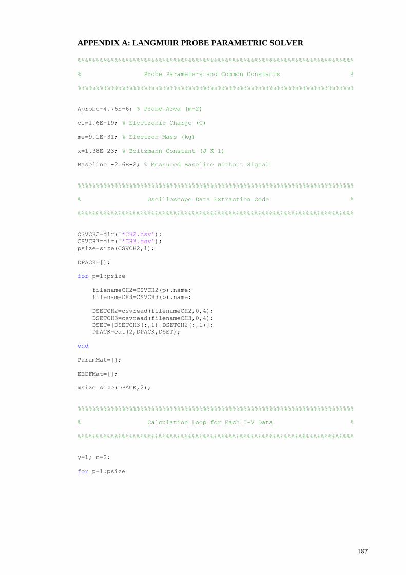
187

APPENDIX A: LANGMUIR PROBE PARAMETRIC SOLVER

%%%%%%%%%%%%%%%%%%%%%%%%%%%%%%%%%%%%%%%%%%%%%%%%%%%%%%%%%%%%%%%%%%%%%%%%%%%

% Probe Parameters and Common Constants %

%%%%%%%%%%%%%%%%%%%%%%%%%%%%%%%%%%%%%%%%%%%%%%%%%%%%%%%%%%%%%%%%%%%%%%%%%%%

Aprobe=4.76E-6; % Probe Area (m-2)

el=1.6E-19; % Electronic Charge (C)

me=9.1E-31; % Electron Mass (kg)

k=1.38E-23; % Boltzmann Constant (J K-1)

Baseline=-2.6E-2; % Measured Baseline Without Signal

%%%%%%%%%%%%%%%%%%%%%%%%%%%%%%%%%%%%%%%%%%%%%%%%%%%%%%%%%%%%%%%%%%%%%%%%%%%

% Oscilloscope Data Extraction Code %

%%%%%%%%%%%%%%%%%%%%%%%%%%%%%%%%%%%%%%%%%%%%%%%%%%%%%%%%%%%%%%%%%%%%%%%%%%%

CSVCH2=dir('*CH2.csv');

CSVCH3=dir('*CH3.csv');

psize=size(CSVCH2,1);

DPACK=[];

for p=1:psize

filenameCH2=CSVCH2(p).name;

filenameCH3=CSVCH3(p).name;

DSETCH2=csvread(filenameCH2,0,4);

DSETCH3=csvread(filenameCH3,0,4);

DSET=[DSETCH3(:,1) DSETCH2(:,1)];

DPACK=cat(2,DPACK,DSET);

end

ParamMat=[];

EEDFMat=[];

msize=size(DPACK,2);

%%%%%%%%%%%%%%%%%%%%%%%%%%%%%%%%%%%%%%%%%%%%%%%%%%%%%%%%%%%%%%%%%%%%%%%%%%%

% Calculation Loop for Each I-V Data %

%%%%%%%%%%%%%%%%%%%%%%%%%%%%%%%%%%%%%%%%%%%%%%%%%%%%%%%%%%%%%%%%%%%%%%%%%%%

y=1; n=2;

for p=1:psize

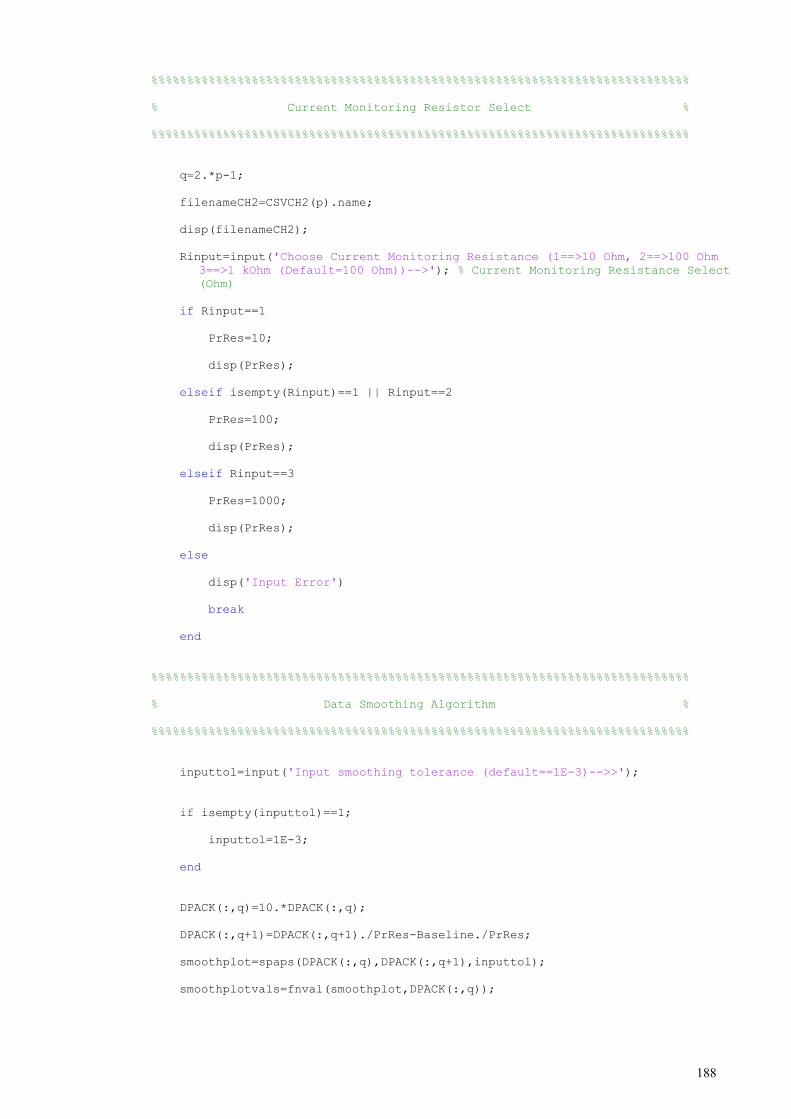
188

%%%%%%%%%%%%%%%%%%%%%%%%%%%%%%%%%%%%%%%%%%%%%%%%%%%%%%%%%%%%%%%%%%%%%%%%%%%

% Current Monitoring Resistor Select %

%%%%%%%%%%%%%%%%%%%%%%%%%%%%%%%%%%%%%%%%%%%%%%%%%%%%%%%%%%%%%%%%%%%%%%%%%%%

q=2.*p-1;

filenameCH2=CSVCH2(p).name;

disp(filenameCH2);

Rinput=input('Choose Current Monitoring Resistance (1==>10 Ohm, 2==>100 Ohm

3==>1 kOhm (Default=100 Ohm))-->'); % Current Monitoring Resistance Select

(Ohm)

if Rinput==1

PrRes=10;

disp(PrRes);

elseif isempty(Rinput)==1 || Rinput==2

PrRes=100;

disp(PrRes);

elseif Rinput==3

PrRes=1000;

disp(PrRes);

else

disp('Input Error')

break

end

%%%%%%%%%%%%%%%%%%%%%%%%%%%%%%%%%%%%%%%%%%%%%%%%%%%%%%%%%%%%%%%%%%%%%%%%%%%

% Data Smoothing Algorithm %

%%%%%%%%%%%%%%%%%%%%%%%%%%%%%%%%%%%%%%%%%%%%%%%%%%%%%%%%%%%%%%%%%%%%%%%%%%%

inputtol=input('Input smoothing tolerance (default==1E-3)-->>');

if isempty(inputtol)==1;

inputtol=1E-3;

end

DPACK(:,q)=10.*DPACK(:,q);

DPACK(:,q+1)=DPACK(:,q+1)./PrRes-Baseline./PrRes;

smoothplot=spaps(DPACK(:,q),DPACK(:,q+1),inputtol);

smoothplotvals=fnval(smoothplot,DPACK(:,q));

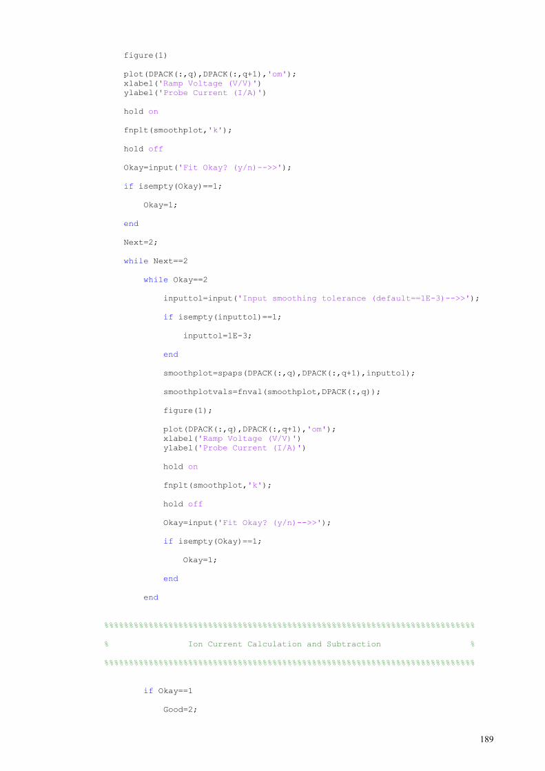
189

figure(1)

plot(DPACK(:,q),DPACK(:,q+1),'om');

xlabel('Ramp Voltage (V/V)')

ylabel('Probe Current (I/A)')

hold on

fnplt(smoothplot,'k');

hold off

Okay=input('Fit Okay? (y/n)-->>');

if isempty(Okay)==1;

Okay=1;

end

Next=2;

while Next==2

while Okay==2

inputtol=input('Input smoothing tolerance (default==1E-3)-->>');

if isempty(inputtol)==1;

inputtol=1E-3;

end

smoothplot=spaps(DPACK(:,q),DPACK(:,q+1),inputtol);

smoothplotvals=fnval(smoothplot,DPACK(:,q));

figure(1);

plot(DPACK(:,q),DPACK(:,q+1),'om');

xlabel('Ramp Voltage (V/V)')

ylabel('Probe Current (I/A)')

hold on

fnplt(smoothplot,'k');

hold off

Okay=input('Fit Okay? (y/n)-->>');

if isempty(Okay)==1;

Okay=1;

end

end

%%%%%%%%%%%%%%%%%%%%%%%%%%%%%%%%%%%%%%%%%%%%%%%%%%%%%%%%%%%%%%%%%%%%%%%%%%%

% Ion Current Calculation and Subtraction %

%%%%%%%%%%%%%%%%%%%%%%%%%%%%%%%%%%%%%%%%%%%%%%%%%%%%%%%%%%%%%%%%%%%%%%%%%%%

if Okay==1

Good=2;

190

while Good==2

figure(1);

plot(DPACK(:,q),DPACK(:,q+1),'om');

xlabel('Ramp Voltage (V/V)')

ylabel('Probe Current (I/A)')

hold on

fnplt(smoothplot,'k');

hold off

disp('Choose Ion Saturation Current Region');

[Vionpoints Iionpoints]=ginput(2);

Iionsat=fnmin(smoothplot,[Vionpoints(1,1) Vionpoints(2,1)]); % Ion

Saturation Current (A)

IonCurrentFit=polyfit(Vionpoints, Iionpoints,1);

IonCurrentVals=IonCurrentFit(1).*DPACK(:,q)+IonCurrentFit(2);

ElectronCurrent=smoothplotvals-IonCurrentVals;

figure(2)

fnplt(smoothplot,'b')

hold on

plot(DPACK(:,q),IonCurrentVals,'g');

plot(DPACK(:,q),ElectronCurrent,'k');

hold off

Good=input('Good Representation? (y/n)-->>');

end

smoothplotelec=spaps(DPACK(:,q),ElectronCurrent,0);

Good=2;

%%%%%%%%%%%%%%%%%%%%%%%%%%%%%%%%%%%%%%%%%%%%%%%%%%%%%%%%%%%%%%%%%%%%%%%%%%%

% Electron Saturation Current Calculation %

%%%%%%%%%%%%%%%%%%%%%%%%%%%%%%%%%%%%%%%%%%%%%%%%%%%%%%%%%%%%%%%%%%%%%%%%%%%

figure(2)

fnplt(smoothplotelec,'k');

while Good==2

disp('Choose Electron Saturation Current Extrapolation Points');

[Velecpoints Ielecpoints]=ginput(2);

[IelecCoeff IelecLin]=polyfit([Velecpoints(1,1)

Velecpoints(2,1)],[fnval(smoothplotelec,Velecpoints(1,1))

fnval(smoothplotelec,Velecpoints(2,1))],1);

IelecLinmin=polyval(IelecCoeff,DPACK(1,q));

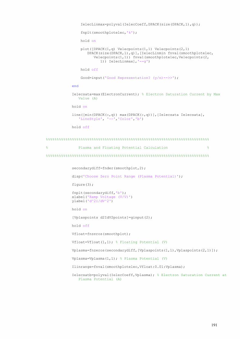
191

IelecLinmax=polyval(IelecCoeff,DPACK(size(DPACK,1),q));

fnplt(smoothplotelec,'k');

hold on

plot([DPACK(1,q) Velecpoints(1,1) Velecpoints(2,1)

DPACK(size(DPACK,1),q)],[IelecLinmin fnval(smoothplotelec,

Velecpoints(1,1)) fnval(smoothplotelec,Velecpoints(2,

1)) IelecLinmax],'--g')

hold off

Good=input('Good Representation? (y/n)-->>');

end

Ielecsata=max(ElectronCurrent); % Electron Saturation Current by Max

Value (A)

hold on

line([min(DPACK(:,q)) max(DPACK(:,q))],[Ielecsata Ielecsata],

'LineStyle', '--','Color','b')

hold off

%%%%%%%%%%%%%%%%%%%%%%%%%%%%%%%%%%%%%%%%%%%%%%%%%%%%%%%%%%%%%%%%%%%%%%%%%%%

% Plasma and Floating Potential Calculation %

%%%%%%%%%%%%%%%%%%%%%%%%%%%%%%%%%%%%%%%%%%%%%%%%%%%%%%%%%%%%%%%%%%%%%%%%%%%

secondarydiff=fnder(smoothplot,2);

disp('Choose Zero Point Range (Plasma Potential)');

figure(3);

fnplt(secondarydiff,'b');

xlabel('Ramp Voltage (V/V)')

ylabel('d^2I/dV^2')

hold on

[Vplaspoints d2IdV2points]=ginput(2);

hold off

Vfloat=fnzeros(smoothplot);

Vfloat=Vfloat(1,1); % Floating Potential (V)

Vplasma=fnzeros(secondarydiff,[Vplaspoints(1,1),Vplaspoints(2,1)]);

Vplasma=Vplasma(1,1); % Plasma Potential (V)

Ilinrange=fnval(smoothplotelec,Vfloat:0.01:Vplasma);

Ielecsatb=polyval(IelecCoeff,Vplasma); % Electron Saturation Current at

Plasma Potential (A)

192

%%%%%%%%%%%%%%%%%%%%%%%%%%%%%%%%%%%%%%%%%%%%%%%%%%%%%%%%%%%%%%%%%%%%%%%%%%%

% Plasma Parameters Calculation %

%%%%%%%%%%%%%%%%%%%%%%%%%%%%%%%%%%%%%%%%%%%%%%%%%%%%%%%%%%%%%%%%%%%%%%%%%%%

TeM=trapz(Vfloat:0.01:Vplasma,Ilinrange)./(fnval(smoothplotelec,

Vplasma)); % Maxwellian Method Electron Temperature (eV)

neM=(fnval(smoothplotelec,Vplasma)./Aprobe).*(2.*pi.*me./(el.^2.*k.*

(TeM*11604.5))).^0.5; % Maxwellian Method Electron Density (m-3)

yDM=743.*(TeM./(neM.*1E-6)).^0.5; % Maxwellian Method Debye Length(m-3)

dEEDF=abs(min(DPACK(:,q)-Vplasma))/2500;

eV=permute(0:dEEDF:abs(min(DPACK(:,q)-Vplasma)),[2 1]);

d2IdV2=permute(fnval(secondarydiff,Vplasma:-dEEDF:min(DPACK(:,q))),[2

1]);

EEDF=(2.*me./(el.^2.*Aprobe)).*(2.*el.*eV./me).^0.5.*d2IdV2; % EEDF(m-3

eV-3/2)

ne=trapz(eV,EEDF);

Teff=2./3.*trapz(eV,eV.*EEDF); % EEDF Method Electron Temperature (eV)

yDeff=743.*(Teff./(ne.*1E-6)).^0.5; % EEDF Method Electron Density(m-3)

figure(4);

plot(eV,EEDF,'b')

xlabel('Electron Energy (E/eV)')

ylabel('EEDF (m-3 eV-3/2)')

else

disp('Input Error');

return

end

Next=input('Next? (y/n)-->>');

if Next==2

Okay=2;

elseif Next==1

ParamMat=cat(1,ParamMat,[p Iionsat Ielecsata Ielecsatb Vplasma Vfloat

neM ne TeM Teff yDM yDeff]);

EEDFMat=cat(2,EEDFMat,[eV EEDF]);

continue

else

disp('Input Error');

return

end

end

end

193

%%%%%%%%%%%%%%%%%%%%%%%%%%%%%%%%%%%%%%%%%%%%%%%%%%%%%%%%%%%%%%%%%%%%%%%%%%%

% Save File Algorithm %

%%%%%%%%%%%%%%%%%%%%%%%%%%%%%%%%%%%%%%%%%%%%%%%%%%%%%%%%%%%%%%%%%%%%%%%%%%%

SaveParamID={'Set', 'Iionsat (A)', 'Ielecsata (A)','Ielecsatb (A)', 'Vplasma (V)',

'Vfloat (V)','neM (m^-3)', 'ne (m^-3)',...

'TeM (eV)', 'Teff (eV)', 'yDM (m)', 'yDeff (m)'};

SaveFile=input('Enter Save Filename -->>','s');

warning off MATLAB:xlswrite:AddSheet

xlswrite([SaveFile,'.xls'],SaveParamID,[SaveFile,' cm'],'A1')

xlswrite([SaveFile,'.xls'],ParamMat,[SaveFile,' cm'],'A2')

xlswrite([SaveFile,'.xls'],{'Average'},[SaveFile,' cm'],['A',num2str(psize+2)]);

xlswrite([SaveFile,'.xls'],{'Standard Deviation'},[SaveFile,'

cm'],['A',num2str(psize+3)]);

xlswrite([SaveFile,'.xls'],mean(ParamMat(:,2:size(ParamMat,2)),1),[SaveFile,'

cm'],['B',num2str(psize+2)]);

xlswrite([SaveFile,'.xls'],std(ParamMat(:,2:size(ParamMat,2)),0,1),[SaveFile,'

cm'],['B',num2str(psize+3)]);

VIString=[];

SetString=[];

EEDFString=[];

for p=1:psize

SetString=cat(2,SetString,{['Set ',num2str(p)],' '});

VIString=cat(2,VIString,{'Voltage,V(V)','Current,I(A)'});

EEDFString=cat(2,EEDFString,{'Electron Energy(eV)','EEDF (m-3 eV-3/2)'});

end

xlswrite([SaveFile,'.xls'],SetString,[SaveFile,' cm'],'O1')

xlswrite([SaveFile,'.xls'],EEDFString,[SaveFile,' cm'],'O2')

xlswrite([SaveFile,'.xls'],EEDFMat,[SaveFile,' cm'],'O3')

xlswrite([SaveFile,'.xls'],SetString,['Raw Data ',SaveFile,' cm'],'A1')

xlswrite([SaveFile,'.xls'],VIString,['Raw Data ',SaveFile,' cm'],'A2')

xlswrite([SaveFile,'.xls'],DPACK,['Raw Data ',SaveFile,' cm'],'A3')

deleteEmptyExcelSheets([cd,'/',SaveFile,'.xls']); % Empty Excel Sheet Delete Code

(Appendix E.3)

disp('Done!')

194

APPENDIX B: AOES Tn SOLVER

This solver is divided into two parts, i.e., B.1 and B.2. Code B.1 must be pre-loaded in

MATLAB workspace before running code B.2. Code B.1 calculates the rotational line

widths and positions for all tested rotational temperatures and convolves the discrete

spectrum with instrumental broadening. Code B.2 extracts experimental data and uses

the minimum 2method to estimate the neutral gas temperature.

---------------------------------------------------------------------------

B.1. AOES Line Width and Line Position Convolution Solver

%%%%%%%%%%%%%%%%%%%%%%%%%%%%%%%%%%%%%%%%%%%%%%%%%%%%%%%%%%%%%%%%%%%%%%%%%%%

% Common Spectroscopy Constants %

%%%%%%%%%%%%%%%%%%%%%%%%%%%%%%%%%%%%%%%%%%%%%%%%%%%%%%%%%%%%%%%%%%%%%%%%%%%

h=6.62606957E-34; % Planck's Constant (m2kgs-1)

c=299792458; % Speed of Light (ms-1)

k=1.3806488E-23; % Boltzmann Constant (JK-1)

nair=1.0003; % Refraction Index of Air

%%%%%%%%%%%%%%%%%%%%%%%%%%%%%%%%%%%%%%%%%%%%%%%%%%%%%%%%%%%%%%%%%%%%%%%%%%%

% Nitrogen Vibro-rotational Constants and Terms %

%%%%%%%%%%%%%%%%%%%%%%%%%%%%%%%%%%%%%%%%%%%%%%%%%%%%%%%%%%%%%%%%%%%%%%%%%%%

% 1 Denotes Upper State, 2 Denotes Lower State %

we1=2047.17;

we2=1733.39;

wexe1=28.445;

wexe2=14.122;

weye1=2.0883;

weye2=-0.0569;

Be1=1.8247;

Be2=1.6374;

alphae1=0.01868;

alphae2=0.0179;

v1=0; % Upper State Vibrational Number

v2=2; % Upper State Vibrational Number

195

A=42.24;

De1=(4.*Be1.^3)/we1.^2;

De2=(4.*Be2.^3)/we2.^2;

betae1=De1.*(8.*wexe1./we1-5.*alphae1./Be1-alphae1.^2.*we1./(24.*Be1.^3));

betae2=De2.*(8.*wexe2./we2-5.*alphae2./Be2-alphae2.^2.*we2./(24.*Be2.^3));

Te1=89136.88; % Upper State Electronic Term (cm-1)

Te2=59619.35; % Lower State Electronic Term (cm-1)

Bv1=Be1-alphae1.*(v1+0.5); % Upper State Rotational Term 1 (cm-1)

Bv2=Be2-alphae2.*(v2+0.5); % Upper State Rotational Term 1 (cm-1)

Dv1=De1+betae1.*(v1+0.5); % Upper State Rotational Term 2 (cm-1)

Dv2=De2+betae2.*(v2+0.5); % Upper State Rotational Term 2 (cm-1)

Gv1=we1.*(v1+0.5)-wexe1.*(v1+0.5).^2+weye1.*(v1+0.5).^3; % Upper State Vibrational

Term (cm-1)

Gv2=we2.*(v2+0.5)-wexe2.*(v2+0.5).^2+weye2.*(v2+0.5).^3; % Lower State Vibrational

Term (cm-1)

Vv1v2=Te1-Te2+Gv1-Gv2;

%%%%%%%%%%%%%%%%%%%%%%%%%%%%%%%%%%%%%%%%%%%%%%%%%%%%%%%%%%%%%%%%%%%%%%%%%%%

% Rotational Line Position/Intensity Calculation Loop %

%%%%%%%%%%%%%%%%%%%%%%%%%%%%%%%%%%%%%%%%%%%%%%%%%%%%%%%%%%%%%%%%%%%%%%%%%%%

ConvSpecGroupStack=[];

TempStart=250; % Starting Rotational Temperature (K)

TempEnd=1500; % Ending Rotational Temperature (K)

dTemp=50; % Spacing Between Temperature Iterations (K)

CorrectedLambd=xlsread('CorrectedLambd.xls'); % Calibrated Spectrometer Wavelength

(Obtained in Calibration Experiment) (nm)

DataSelect=CorrectedLambd(1380:1418); % Wavelength Range of Selected (0-2) Peak

for Trot=TempStart:dTemp:TempEnd;

disp(['Fit Calculation for Temperature =',num2str(Trot), ' K'])

SynSpecMat=[];

for JR=0:50 % R Rotational Branch Calculations

FvR1D0=Bv1.*(JR+1).*(JR+2)-Dv1.*(JR+1).^2.*(JR+2).^2;

FvR2D0=Bv2.*JR.*(JR+1)-Dv2.*JR.^2.*(JR+1).^2;

VRD0=Vv1v2+FvR1D0-FvR2D0;

LRD0=1E-2./(VRD0.*nair);

SJRD0=JR+1;

IREmissD0=SJRD0.*exp(-100.*FvR1D0.*h.*c./(k.*Trot));

196

if JR>=1

FvR1D1=Bv1.*((JR+1).*(JR+2)-1)-Dv1.*(JR+1).^2.*(JR+2).^2+A;

FvR2D1=Bv2.*(JR.*(JR+1)-1)-Dv2.*JR.^2.*(JR+1).^2+A;

VRD1=Vv1v2+FvR1D1-FvR2D1;

LRD1=1E-2./(VRD1.*nair);

SJRD1=((JR+1).^2-1)./(JR+1);

IREmissD1=SJRD1.*exp(-100.*FvR1D1.*h.*c./(k.*Trot));

else

LRD1=[];

SJRD1=[];

IREmissD1=[];

end

if JR>=2

FvR1D2=Bv1.*((JR+1).*(JR+2)-4)- Dv1.*(JR+1).^2.*(JR+2).^2+

4.*A;

FvR2D2=Bv2.*(JR.*(JR+1)-4)-Dv2.*JR.^2.*(JR+1).^2+4.*A;

VRD2=Vv1v2+FvR1D2-FvR2D2;

LRD2=1E-2./(VRD2.*nair);

SJRD2=((JR+1).^2-4)./(JR+1);

IREmissD2=SJRD2.*exp(-100.*FvR1D2.*h.*c./(k.*Trot));

else

LRD2=[];

SJRD2=[];

IREmissD2=[];

end

SynSpecSeg=[LRD0 IREmissD0 SJRD0; LRD1 IREmissD1 SJRD1; LRD2

IREmissD2 SJRD2];

SynSpecMat=cat(1, SynSpecMat,SynSpecSeg);

end

for JQ=1:50 % Q Rotational Branch Calculations

FvQ1D0=Bv1.*JQ.*(JQ+1)-Dv1.*JQ.^2.*(JQ+1).^2;

FvQ2D0=Bv2.*JQ.*(JQ+1)-Dv2.*JQ.^2.*(JQ+1).^2;

VQD0=Vv1v2+FvQ1D0-FvQ2D0;

LQD0=[];

SJQD0=[];

IQEmissD0=[];

FvQ1D1=Bv1.*(JQ.*(JQ+1)-1)-Dv1.*JQ.^2.*(JQ+1).^2+A;

197

FvQ2D1=Bv2.*(JQ.*(JQ+1)-1)-Dv2.*JQ.^2.*(JQ+1).^2+A;

VQD1=Vv1v2+FvQ1D1-FvQ2D1;

LQD1=1E-2./(VQD1.*nair);

SJQD1=(2.*JQ+1)./(JQ.*(JQ+1));

IQEmissD1=SJQD1.*exp(-100.*FvQ1D1.*h.*c./(k.*Trot));

if JQ>=2

FvQ1D2=Bv1.*(JQ.*(JQ+1)-4)-Dv1.*JQ.^2.*(JQ+1).^2+4.*A;

FvQ2D2=Bv2.*(JQ.*(JQ+1)-4)-Dv2.*JQ.^2.*(JQ+1).^2+4.*A;

VQD2=Vv1v2+FvQ1D2-FvQ2D2;

LQD2=1E-2./(VQD2.*nair);

SJQD2=4.*(2.*JQ+1)./(JQ.*(JQ+1));

IQEmissD2=SJQD2.*exp(-100.*FvQ1D2.*h.*c./(k.*Trot));

else

LQD2=[];

SJQD2=[];

IQEmissD2=[];

end

SynSpecSeg=[LQD0 IQEmissD0 SJQD0; LQD1 IQEmissD1 SJQD1; LQD2

IQEmissD2 SJQD2];

SynSpecMat=cat(1, SynSpecMat,SynSpecSeg);

end

for JP=1:50 % P Rotational Branch Calculations

FvP1D0=Bv1.*JP.*(JP-1)-Dv1.*JP.^2.*(JP-1).^2;

FvP2D0=Bv2.*JP.*(JP+1)-Dv2.*JP.^2.*(JP+1).^2;

VPD0=Vv1v2+FvP1D0-FvP2D0;

LPD0=1E-2./(VPD0.*nair);

SJPD0=JP;

IPEmissD0=SJPD0.*exp(-100.*FvP1D0.*h.*c./(k.*Trot));

if JP>=2

FvP1D1=Bv1.*(JP.*(JP-1)-1)-Dv1.*JP.^2.*(JP-1).^2+A;

FvP2D1=Bv2.*(JP.*(JP+1)-1)-Dv2.*JP.^2.*(JP+1).^2+A;

VPD1=Vv1v2+FvP1D1-FvP2D1;

LPD1=1E-2./(VPD1.*nair);

SJPD1=(JP+1).*(JP-1)./JP;

IPEmissD1=SJPD1.*exp(-100.*FvP1D1.*h.*c./(k.*Trot));

198

else

LPD1=[];

SJPD1=[];

IPEmissD1=[];

end

if JP>=3

FvP1D2=Bv1.*(JP.*(JP-1)-4)-Dv1.*JP.^2.*(JP-1).^2+4.*A;

FvP2D2=Bv2.*(JP.*(JP+1)-4)-Dv2.*JP.^2.*(JP+1).^2+4.*A;

VPD2=Vv1v2+FvP1D2-FvP2D2;

LPD2=1E-2./(VPD2.*nair);

SJPD2=(JP+2).*(JP-2)./JP;

IPEmissD2=SJPD2.*exp(-100.*FvP1D2.*h.*c./(k.*Trot));

else

LPD2=[];

SJPD2=[];

IPEmissD2=[];

end

SynSpecSeg=[LPD0 IPEmissD0 SJPD0; LPD1 IPEmissD1 SJPD1; LPD2

IPEmissD2 SJPD2];

SynSpecMat=cat(1, SynSpecMat,SynSpecSeg);

end

SynSpecMat=sortrows(SynSpecMat,1);

%%%%%%%%%%%%%%%%%%%%%%%%%%%%%%%%%%%%%%%%%%%%%%%%%%%%%%%%%%%%%%%%%%%%%%%%%%%

% Voigt Profile Matrix Loop %

%%%%%%%%%%%%%%%%%%%%%%%%%%%%%%%%%%%%%%%%%%%%%%%%%%%%%%%%%%%%%%%%%%%%%%%%%%%

% Voigt Profile Broadening is Calculated for Wavelengths/Line Positions and Column-

stacked as a Matrix %

dDataSelect=abs(DataSelect(1,1)-DataSelect(2,1)); % Spectrometer

Pixel Resolution (nm)

dLambd=4*dDataSelect; % Bin Size (nm)

LambdSynSpec=SynSpecMat(:,1)./1E-9;

LambdAdd=permute(max(LambdSynSpec)+0.01:0.01:round(max(LambdSynSpec)

)+1,[2 1]);

LambdFullSynSpec=cat(1,LambdSynSpec,LambdAdd);

IntSynSpec=SynSpecMat(:,2);

IntAdd=zeros(numel(LambdAdd),1);

IntFullSynSpec=cat(1,IntSynSpec,IntAdd);

199

LambdGroup=min(DataSelect(:,1)):dLambd:max(DataSelect(:,1));

ConvSpecGroup=zeros(1,numel(LambdGroup));

VoiGroup=[];

FWHMLor=0.6; % Lorentz FWHM

FWHMGau=0.5; % Gaussian FWHM

for n=1:numel(LambdFullSynSpec)

FWHMVoi=FWHMLor./2+sqrt(FWHMLor.^2./4+FWHMGau.^2); % Voigt FWHM

VoiNorm=real((1-FWHMLor./FWHMVoi).*exp(-

4.*log(2).*((LambdFullSynSpec-LambdFullSynSpec(n))

./FWHMVoi).^2)+(FWHMLor./FWHMVoi).*(1./(1+4.*

((LambdFullSynSpec-LambdFullSynSpec(n))

./FWHMVoi).^2))+0.016.*(1-FWHMLor./FWHMVoi)

.*(FWHMLor./FWHMVoi).*(exp(- 0.4

.*((LambdFullSynSpec-LambdFullSynSpec(n))

./FWHMVoi).^2.25)-10./(10+((LambdFullSyn

Spec-LambdFullSynSpec(n))./FWHMVoi)

.^2.25)));

VoiGroup=cat(2,VoiGroup,permute(VoiNorm,[1 2]));

end

%%%%%%%%%%%%%%%%%%%%%%%%%%%%%%%%%%%%%%%%%%%%%%%%%%%%%%%%%%%%%%%%%%%%%%%%%%%

% Bin Probability Calculation for Minimum Chi-Squared Method (B.2) %

%%%%%%%%%%%%%%%%%%%%%%%%%%%%%%%%%%%%%%%%%%%%%%%%%%%%%%%%%%%%%%%%%%%%%%%%%%%

LineSum=zeros(numel(LambdGroup),1);

for n=1:numel(LambdFullSynSpec)

for p=1:numel(LambdGroup);

if LambdFullSynSpec(n)>=LambdGroup(p)-

dLambd/2&&LambdFullSynSpec(n) <LambdGroup(p)+dLambd/2

LineSum(p)=LineSum(p)+1;

else

end

end

end

LineProb=LineSum./sum(LineSum); % Line Probability for Bins

%%%%%%%%%%%%%%%%%%%%%%%%%%%%%%%%%%%%%%%%%%%%%%%%%%%%%%%%%%%%%%%%%%%%%%%%%%%

% Convolution Matrix Loop %

%%%%%%%%%%%%%%%%%%%%%%%%%%%%%%%%%%%%%%%%%%%%%%%%%%%%%%%%%%%%%%%%%%%%%%%%%%%

for m=1:numel(LambdFullSynSpec)

ConvSpecStack=[];

200

ConvIntSpec=zeros(numel(LambdFullSynSpec),1);

ConvIntSpec(m)=IntFullSynSpec(m);

for n=1:numel(LambdFullSynSpec)

ConvSpec=trapz(LambdFullSynSpec,ConvIntSpec.*VoiGroup(:,n));

ConvSpecStack=cat(1,ConvSpecStack, ConvSpec);

for p=1:numel(LambdGroup);

if LambdFullSynSpec(n)>=LambdGroup(p)-dLambd/2&&

LambdFullSynSpec(n)<LambdGroup(p)+dLambd/2

ConvSpecGroup(p)=ConvSpecGroup(p)+ConvSpec;

else

end

end

end

end

ConvSpecGroupNorm=permute(ConvSpecGroup./max(ConvSpecGroup),[2 1]);

ConvSpecGroupStack=cat(2,ConvSpecGroupStack,permute(ConvSpecGroup

Norm, [1 2])); % Normalized Convolved Spectrum Stack for

Rotational Temperature Range

end

disp('Done!')

201

B.2. AOES Minimum 2

Neutral Gas Temperature Solver

%%%%%%%%%%%%%%%%%%%%%%%%%%%%%%%%%%%%%%%%%%%%%%%%%%%%%%%%%%%%%%%%%%%%%%%%%%%

% Definition of Set Plasma Parameters %

%%%%%%%%%%%%%%%%%%%%%%%%%%%%%%%%%%%%%%%%%%%%%%%%%%%%%%%%%%%%%%%%%%%%%%%%%%%

TempMatrix=[];

ArgPres=input('Input Argon Pressure ----->'); % Set Argon Pressure for Save File

AxialH=input('Input Axial Height ----->'); % Set Axial Height for Save File

DataCollect=dir('*.txt'); % Collection of ASCII (*.txt) Output Files from

SpectraSuite Software

DataCollSize=size(DataCollect,1);

%%%%%%%%%%%%%%%%%%%%%%%%%%%%%%%%%%%%%%%%%%%%%%%%%%%%%%%%%%%%%%%%%%%%%%%%%%%

% Data Filename Sorter %

%%%%%%%%%%%%%%%%%%%%%%%%%%%%%%%%%%%%%%%%%%%%%%%%%%%%%%%%%%%%%%%%%%%%%%%%%%%

% This Code Extracts and Sorts Data Files According to Parameters Labeled in

Filename. %

% Filename Should Have the Following Format:'[R.f. Power][Plasma Mode]*.txt' for

Code to Work, e.g. 180WHmode*.txt %

% 20 Data Sets were Obtained for Each Measured Point. %

PlasPowMat=[];

for dc=1:DataCollSize

DataCollName=DataCollect(dc).name;

PPVal1=num2str(str2num(DataCollName(1)));

PPVal2=num2str(str2num(DataCollName(2)));

PPVal3=num2str(str2num(DataCollName(3)));

PlasPowComp=str2num(strcat(PPVal1,PPVal2,PPVal3));

PPMatSize=numel(PlasPowMat);

if isempty(PlasPowMat)==1;

PlasPowMat=cat(2,PlasPowMat,PlasPowComp);

elseif PlasPowComp==PlasPowMat(PPMatSize);

else

PlasPowMat=cat(2,PlasPowMat,PlasPowComp);

end

end

PlasPowMat=sort(PlasPowMat);

for PlasmPower=PlasPowMat % Sorting by R.f. Power and Plasma Mode

202

DataGroup=dir([num2str(PlasmPower),'W*.txt']);

DataSize=size(DataGroup,1);

DataSelect=CorrectedLambd(1380:1418); % 0-2) Peak Calibrated Wavelength Range

(nm)

for dt=1:DataSize

DataName=DataGroup(dt).name;

for dn=1:numel(DataName);

if DataName(dn)=='H'

PlasmaType={'H'};

disp('H-mode');

elseif DataName(dn)=='E'

PlasmaType={'E'};

disp('E-mode');

else

end

end

disp(DataName);

DataAqui=dlmread(DataName,'\t',[17 1 3664 1]);

DataSet=DataAqui(1380:1418); % (0-2) Peak Intensity Data From File

DataSet=DataSet-min(DataSet); % Removal of Background Emission Noise

DataSet=DataSet./max(DataSet); % Normalizing of (0-2) Peak Intensity Data

DataSelect=cat(2,DataSelect,DataSet); % Stacking of Acquired and Processed

Data

end

%%%%%%%%%%%%%%%%%%%%%%%%%%%%%%%%%%%%%%%%%%%%%%%%%%%%%%%%%%%%%%%%%%%%%%%%%%%

% Minimum Chi-Squared Loop %

%%%%%%%%%%%%%%%%%%%%%%%%%%%%%%%%%%%%%%%%%%%%%%%%%%%%%%%%%%%%%%%%%%%%%%%%%%%

Chi2Stack=[];

for Tmp=1:size(ConvSpecGroupStack,2);

DataNum=numel(LambdGroup);

Chi2StackH=[];

for n=1:DataSize

DataSelectChi=permute(interp1(DataSelect(:,1),

DataSelect(:,n+1),LambdGroup),[2 1]);

Chi2Val=sum(LineProb.*(DataSelectChi-

ConvSpecGroupStack(:,Tmp)).^2)./(DataNum.*(DataNum-1));

203

Chi2StackH=cat(2,Chi2StackH,Chi2Val);

end

Chi2Stack=cat(1,Chi2Stack,Chi2StackH);

end

NeutralTemp=TempStart:dTemp:TempEnd;

TempDataSet=[];

for n=1:DataSize

figure(1) % Chi-Squared Curve

plot(NeutralTemp, Chi2Stack(:,n), 'o');

xlabel('Neutral Gas Temperature, T_n (K)')

ylabel('X^2 (arb. units)')

[MinChi2 MinChi2I]=min(Chi2Stack(:,n));

MinFitTemp=NeutralTemp(MinChi2I);

TempDataSet=cat(1,TempDataSet,MinFitTemp);

disp(['Estimated Neutral Temperature = ',num2str(MinFitTemp), ' K'])

figure(2) % Measured and Convolved(0-2)Peaks at Best Fitted Temperature

plot(LambdGroup,ConvSpecGroupStack(:,MinChi2I),'k');

xlabel('Wavelength (nm)')

ylabel('Intensity (arb. units)')

ylim([0 max(ConvSpecGroupStack(:,MinChi2I))]);

hold on

plot(DataSelect(:,1),DataSelect(:,n+1),'or');

hold off

end

TempAve=mean(TempDataSet); % Mean Temerature for 20 Data Sets at Measured Point

TempStd=std(TempDataSet); % Standard Deviation for 20 Data Sets at Measured

Point

TempMatrix=cat(1,TempMatrix,[PlasmPower TempAve TempStd]); % Save File Matrix

Stack

end

%%%%%%%%%%%%%%%%%%%%%%%%%%%%%%%%%%%%%%%%%%%%%%%%%%%%%%%%%%%%%%%%%%%%%%%%%%%

% Save File Algorithm %

%%%%%%%%%%%%%%%%%%%%%%%%%%%%%%%%%%%%%%%%%%%%%%%%%%%%%%%%%%%%%%%%%%%%%%%%%%%

warning off MATLAB:xlswrite:AddSheet

TempID={'Plasma Power (W)','Average Neutral Temperature (K)', 'Standard Deviation

(K)'};

xlswrite([num2str(AxialH),' cm Neutral Gas Temperature Data.xls'],

TempID,[num2str(ArgPres), ' mbar '],'A1');

204

xlswrite([num2str(AxialH),' cm Neutral Gas Temperature Data.xls'],

TempMatrix,[num2str(ArgPres), ' mbar '],'A2');

deleteEmptyExcelSheets([cd,'/',num2str(AxialH),' cm Neutral Gas Temperature

Data.xls']); % Empty Excel Sheet Delete Code (Appendix E.3)

disp('Done!')

205

APPENDIX C: ANALYTICAL H MODE FIELD MODEL

%%%%%%%%%%%%%%%%%%%%%%%%%%%%%%%%%%%%%%%%%%%%%%%%%%%%%%%%%%%%%%%%%%%%%%%%%%%

% Chamber and Coil Dimensions %

%%%%%%%%%%%%%%%%%%%%%%%%%%%%%%%%%%%%%%%%%%%%%%%%%%%%%%%%%%%%%%%%%%%%%%%%%%%

L=21.8E-2; % Effective Chamber Height (m)

D=2.4E-2; % Chamber-Coil Spacing (m)

b=14.5E-2; % Chamber Radius (m)

a=4.5E-2; % Planar Coil Radius (m)

N=6; % Number of Coil Turns

%%%%%%%%%%%%%%%%%%%%%%%%%%%%%%%%%%%%%%%%%%%%%%%%%%%%%%%%%%%%%%%%%%%%%%%%%%%

% Iteration Parameters and Boundary Conditions %

%%%%%%%%%%%%%%%%%%%%%%%%%%%%%%%%%%%%%%%%%%%%%%%%%%%%%%%%%%%%%%%%%%%%%%%%%%%

dr=0.5E-2; % Radial Iteration Spacing (m)

dri=0.1E-2; % Interpolated Radial Spacing (m)

dz=0.5E-2; % Axial Iteration Spacing (m)

dzi=0.1E-2; % Interpolated Axial Spacing (m)

[r,z]=meshgrid(-b:dr:b,0:dz:L+D); % Field Grid Allocation (m)

[ri zi]=meshgrid(-b:dri:b,0:dzi:L+D); % Interpolated Field Grid (m)

rlim=size(r,2); % Radial Limit

zlimL=size(0:dz:L,2); % Reactor Axial Limit

zlimLD=size(0:dz:L+D,2); % Reactor-Coil Axial Limit

%%%%%%%%%%%%%%%%%%%%%%%%%%%%%%%%%%%%%%%%%%%%%%%%%%%%%%%%%%%%%%%%%%%%%%%%%%%

% R.f. Parameters and Constants %

%%%%%%%%%%%%%%%%%%%%%%%%%%%%%%%%%%%%%%%%%%%%%%%%%%%%%%%%%%%%%%%%%%%%%%%%%%%

f=13.56E6; % RF Frequency (Hz)

w=2.*pi.*f; % RF Angular Frequency (rad s-1)

Irms=13.9; % RMS Coil Current (A)

Ip=Irms.*(2.^0.5); % Peak Coil Current (A)

%%%%%%%%%%%%%%%%%%%%%%%%%%%%%%%%%%%%%%%%%%%%%%%%%%%%%%%%%%%%%%%%%%%%%%%%%%%

% Plasma and EM Field Physical Constants and Parameters %

%%%%%%%%%%%%%%%%%%%%%%%%%%%%%%%%%%%%%%%%%%%%%%%%%%%%%%%%%%%%%%%%%%%%%%%%%%%

ne=5E17; % Electron Density (m-3)

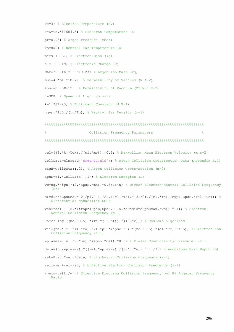
206

Te=3; % Electron Temperature (eV)

TeK=Te.*11604.5; % Electron Temperature (K)

pr=0.03; % Argon Pressure (mbar)

Tn=800; % Neutral Gas Temperature (K)

me=9.1E-31; % Electron Mass (kg)

el=1.6E-19; % Electronic Charge (C)

MAr=39.948.*1.661E-27; % Argon Ion Mass (kg)

muo=4.*pi.*1E-7; % Permeability of Vaccuum (N A-2)

epso=8.85E-12; % Permittivity of Vaccuum (C2 N-1 m-2)

c=3E8; % Speed of Light (m s-1)

k=1.38E-23; % Boltzmann Constant (J K-1)

ng=pr*100./(k.*Tn); % Neutral Gas Density (m-3)

%%%%%%%%%%%%%%%%%%%%%%%%%%%%%%%%%%%%%%%%%%%%%%%%%%%%%%%%%%%%%%%%%%%%%%%%%%%

% Collision Frequency Parameters %

%%%%%%%%%%%%%%%%%%%%%%%%%%%%%%%%%%%%%%%%%%%%%%%%%%%%%%%%%%%%%%%%%%%%%%%%%%%

vel=((8.*k.*TeK)./(pi.*me)).^0.5; % Maxwellian Mean Electron Velocity (m s-2)

CollData=xlsread('ArgonCC.xls'); % Argon Collision Crosssection Data (Appendix E.1)

sigH=CollData(:,2); % Argon Collision Cross-Section (m-2)

EpsE=el.*CollData(:,1); % Electron Energies (J)

vc=ng.*sigH.*(2.*EpsE./me).^0.5+1i*w; % Direct Electron-Neutral Collision Frequency

(Hz)

dFedistdEpsEMax=-2./pi.^(1./2)./(el.*Te).^(3./2)./(el.*Te).*exp(-EpsE./(el.*Te)); %

Differential Maxwellian EEDF

ven=real(-1.5.*(trapz(EpsE,EpsE.^1.5.*dFedistdEpsEMax./vc)).^-1); % Electron-

Neutral Collision Frequency (s-1)

CA=23-log(((ne.^0.5).*(Te.^(-1.5)))./(10.^2)); % Coulomb Algorithm

vei=(ne.*(el.^4).*CA)./(4.*pi.*(epso.^2).*(me.^0.5).*(el.*Te).^1.5); % Electron-Ion

Collision Frequency (s-1)

wplasma=((el.^2.*ne)./(epso.*me)).^0.5; % Plasma Conductivity Parameter (s-1)

dela=(c./wplasma).*((vel.*wplasma)./(2.*c.*w)).^(1./3); % Anomalous Skin Depth (m)

vst=0.25.*vel./dela; % Stochastic Collision Frequency (s-1)

veff=ven+vei+vst; % Effective Electron Collision Frequency (s-1)

vperw=veff./w; % Effective Electron Collision Frequency per RF Angular Frequency

Ratio

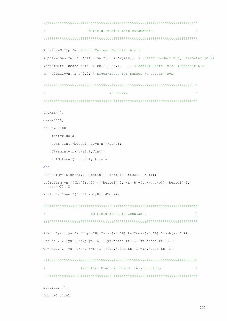
207

%%%%%%%%%%%%%%%%%%%%%%%%%%%%%%%%%%%%%%%%%%%%%%%%%%%%%%%%%%%%%%%%%%%%%%%%%%%

% EM Field Initial Loop Parameters %

%%%%%%%%%%%%%%%%%%%%%%%%%%%%%%%%%%%%%%%%%%%%%%%%%%%%%%%%%%%%%%%%%%%%%%%%%%%

Kthetha=N.*Ip./a; % Coil Current Density (A m-1)

alpha2=(muo.*el.^2.*ne)./(me.*(1-1i.*vperw)); % Plasma Conductivity Parameter (m-2)

yn=permute((besselzero(1,100,1))./b,[2 1]); % Bessel Roots (m-2) (Appendix E.2)

kn=(alpha2+yn.^2).^0.5; % Eigenvalues for Bessel Functions (m-2)

%%%%%%%%%%%%%%%%%%%%%%%%%%%%%%%%%%%%%%%%%%%%%%%%%%%%%%%%%%%%%%%%%%%%%%%%%%%

% vn Solver %

%%%%%%%%%%%%%%%%%%%%%%%%%%%%%%%%%%%%%%%%%%%%%%%%%%%%%%%%%%%%%%%%%%%%%%%%%%%

IntMat=[];

da=a/1000;

for n=1:100

rint=0:da:a;

Jint=rint.*besselj(1,yn(n).*rint);

Jtermint=trapz(rint,Jint);

IntMat=cat(1,IntMat,Jtermint);

end

IntJTerm=-(Kthetha./(1+betan)).*permute(IntMat, [2 1]);

DiffJTerm=yn.*((b.^2)./2).*((besselj(0, yn.*b)-(1./(yn.*b)).*besselj(1,

yn.*b)).^2);

vn=1i.*w.*muo.*(IntJTerm./DiffJTerm);

%%%%%%%%%%%%%%%%%%%%%%%%%%%%%%%%%%%%%%%%%%%%%%%%%%%%%%%%%%%%%%%%%%%%%%%%%%%

% EM Field Boundary Constants %

%%%%%%%%%%%%%%%%%%%%%%%%%%%%%%%%%%%%%%%%%%%%%%%%%%%%%%%%%%%%%%%%%%%%%%%%%%%

An=vn.*yn./(yn.*sinh(yn.*D).*sinh(kn.*L)+kn.*cosh(kn.*L).*cosh(yn.*D));

Bn=(An./(2.*yn)).*exp(yn.*L).*(yn.*sinh(kn.*L)-kn.*cosh(kn.*L));

Cn=(An./(2.*yn)).*exp(-yn.*L).*(yn.*sinh(kn.*L)+kn.*cosh(kn.*L));

%%%%%%%%%%%%%%%%%%%%%%%%%%%%%%%%%%%%%%%%%%%%%%%%%%%%%%%%%%%%%%%%%%%%%%%%%%%

% Azimuthal Electric Field Iteration Loop %

%%%%%%%%%%%%%%%%%%%%%%%%%%%%%%%%%%%%%%%%%%%%%%%%%%%%%%%%%%%%%%%%%%%%%%%%%%%

Ethethaz=[];

for m=1:zlimL

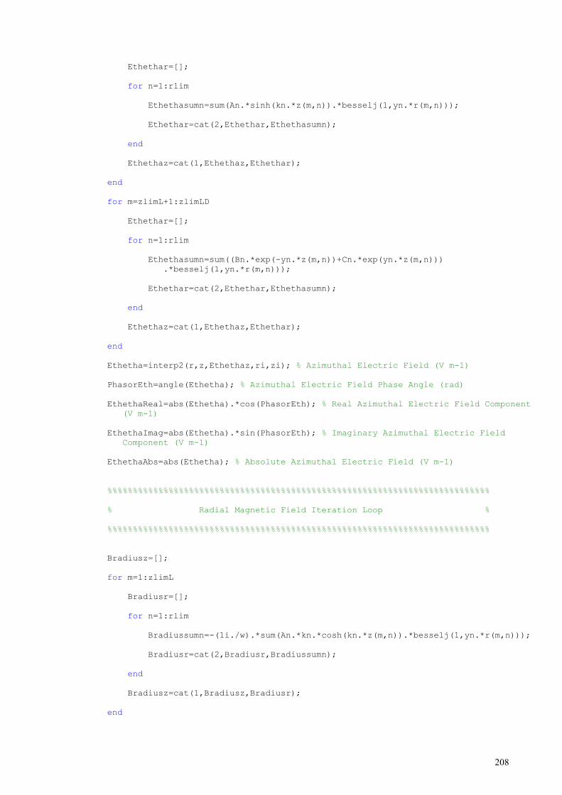
208

Ethethar=[];

for n=1:rlim

Ethethasumn=sum(An.*sinh(kn.*z(m,n)).*besselj(1,yn.*r(m,n)));

Ethethar=cat(2,Ethethar,Ethethasumn);

end

Ethethaz=cat(1,Ethethaz,Ethethar);

end

for m=zlimL+1:zlimLD

Ethethar=[];

for n=1:rlim

Ethethasumn=sum((Bn.*exp(-yn.*z(m,n))+Cn.*exp(yn.*z(m,n)))

.*besselj(1,yn.*r(m,n)));

Ethethar=cat(2,Ethethar,Ethethasumn);

end

Ethethaz=cat(1,Ethethaz,Ethethar);

end

Ethetha=interp2(r,z,Ethethaz,ri,zi); % Azimuthal Electric Field (V m-1)

PhasorEth=angle(Ethetha); % Azimuthal Electric Field Phase Angle (rad)

EthethaReal=abs(Ethetha).*cos(PhasorEth); % Real Azimuthal Electric Field Component

(V m-1)

EthethaImag=abs(Ethetha).*sin(PhasorEth); % Imaginary Azimuthal Electric Field

Component (V m-1)

EthethaAbs=abs(Ethetha); % Absolute Azimuthal Electric Field (V m-1)

%%%%%%%%%%%%%%%%%%%%%%%%%%%%%%%%%%%%%%%%%%%%%%%%%%%%%%%%%%%%%%%%%%%%%%%%%%%

% Radial Magnetic Field Iteration Loop %

%%%%%%%%%%%%%%%%%%%%%%%%%%%%%%%%%%%%%%%%%%%%%%%%%%%%%%%%%%%%%%%%%%%%%%%%%%%

Bradiusz=[];

for m=1:zlimL

Bradiusr=[];

for n=1:rlim

Bradiussumn=-(1i./w).*sum(An.*kn.*cosh(kn.*z(m,n)).*besselj(1,yn.*r(m,n)));

Bradiusr=cat(2,Bradiusr,Bradiussumn);

end

Bradiusz=cat(1,Bradiusz,Bradiusr);

end

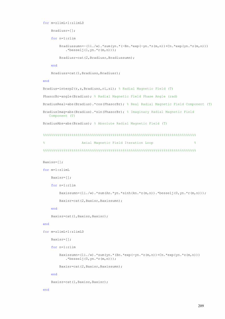
209

for m=zlimL+1:zlimLD

Bradiusr=[];

for n=1:rlim

Bradiussumn=-(1i./w).*sum(yn.*(-Bn.*exp(-yn.*z(m,n))+Cn.*exp(yn.*z(m,n)))

.*besselj(1,yn.*r(m,n)));

Bradiusr=cat(2,Bradiusr,Bradiussumn);

end

Bradiusz=cat(1,Bradiusz,Bradiusr);

end

Bradius=interp2(r,z,Bradiusz,ri,zi); % Radial Magnetic Field (T)

PhasorBr=angle(Bradius); % Radial Magnetic Field Phase Angle (rad)

BradiusReal=abs(Bradius).*cos(PhasorBr); % Real Radial Magnetic Field Component (T)

BradiusImag=abs(Bradius).*sin(PhasorBr); % Imaginary Radial Magnetic Field

Component (T)

BradiusAbs=abs(Bradius); % Absolute Radial Magnetic Field (T)

%%%%%%%%%%%%%%%%%%%%%%%%%%%%%%%%%%%%%%%%%%%%%%%%%%%%%%%%%%%%%%%%%%%%%%%%%%%

% Axial Magnetic Field Iteration Loop %

%%%%%%%%%%%%%%%%%%%%%%%%%%%%%%%%%%%%%%%%%%%%%%%%%%%%%%%%%%%%%%%%%%%%%%%%%%%

Baxisz=[];

for m=1:zlimL

Baxisr=[];

for n=1:rlim

Baxissumn=(1i./w).*sum(An.*yn.*sinh(kn.*z(m,n)).*besselj(0,yn.*r(m,n)));

Baxisr=cat(2,Baxisr,Baxissumn);

end

Baxisz=cat(1,Baxisz,Baxisr);

end

for m=zlimL+1:zlimLD

Baxisr=[];

for n=1:rlim

Baxissumn=(1i./w).*sum(yn.*(Bn.*exp(-yn.*z(m,n))+Cn.*exp(yn.*z(m,n)))

.*besselj(0,yn.*r(m,n)));

Baxisr=cat(2,Baxisr,Baxissumn);

end

Baxisz=cat(1,Baxisz,Baxisr);

end

210

Baxis=interp2(r,z,Baxisz,ri,zi); % Axial Magnetic Field (T)

PhasorBz=angle(Baxis); % Axial Magnetic Field Phase Angle (rad)

BaxisReal=abs(Baxis).*cos(PhasorBz); % Real Axial Magnetic Field Component (T)

BaxisImag=abs(Baxis).*sin(PhasorBz); % Imaginary Axial Magnetic Field Component (T)

BaxisAbs=abs(Baxis); % Absolute Axial Magnetic Field (T)

%%%%%%%%%%%%%%%%%%%%%%%%%%%%%%%%%%%%%%%%%%%%%%%%%%%%%%%%%%%%%%%%%%%%%%%%%%%

% Total Magnetic Field %

%%%%%%%%%%%%%%%%%%%%%%%%%%%%%%%%%%%%%%%%%%%%%%%%%%%%%%%%%%%%%%%%%%%%%%%%%%%

Bfield=(Bradius.^2+Baxis.^2).^0.5; % Total Magnetic Field (T)

PhasorBf=angle(Bfield); % Total Magnetic Field Phase Angle (rad)

BfieldReal=abs(Bfield).*cos(PhasorBf); % Real Total Magnetic Field Component (T)

BfieldImag=abs(Bfield).*sin(PhasorBf); % Imaginary Total Magnetic Field Component

(T)

BfieldAbs=abs(Bfield); % Absolute Total Magnetic Field (T)

%%%%%%%%%%%%%%%%%%%%%%%%%%%%%%%%%%%%%%%%%%%%%%%%%%%%%%%%%%%%%%%%%%%%%%%%%%%

% Magnetic Vector Potential for Contour Plot (Additional Feature) %

%%%%%%%%%%%%%%%%%%%%%%%%%%%%%%%%%%%%%%%%%%%%%%%%%%%%%%%%%%%%%%%%%%%%%%%%%%%

rAthetha=(1i./w).*(ri.*Ethetha); % Azimuthal Magnetic Vector Potential (A)

rAthethaAbs=abs(rAthetha); % Absolute Azimuthal Magnetic Vector Potential (A)

PhasorrAth=angle(rAthetha); % Azimuthal Magnetic Vector Phase Angle (rad)

%%%%%%%%%%%%%%%%%%%%%%%%%%%%%%%%%%%%%%%%%%%%%%%%%%%%%%%%%%%%%%%%%%%%%%%%%%%

% Field Animation and Contour Plot %

%%%%%%%%%%%%%%%%%%%%%%%%%%%%%%%%%%%%%%%%%%%%%%%%%%%%%%%%%%%%%%%%%%%%%%%%%%%

T=(2.*pi)./w; % R.f. Oscillation Period (s)

t=T/100; % Time Capture Interval (s)

timeplot=0:t:2*T;

timelim=size(timeplot,2);

FieldType=input('Select Field Animation Plot: \n [1] Electric Field Distribution \n

[2] Magnetic Field Distribution \n [3] Magnetic Field Contour Plot \n \n --> ');

if FieldType==1

PlotLimitE=max((max(EthethaAbs)));

for j=1:timelim

surf(ri,zi,EthethaAbs.*cos(w.*timeplot(j)+PhasorEth),'EdgeColor','none')

colormap(jet (256))

colorbar('EastOutside')

211

caxis([-PlotLimitE PlotLimitE])

xlim([-b b])

ylim([0 L+D])

zlim([-1.2.*PlotLimitE 1.2.*PlotLimitE])

view(180,90)

F(j)=getframe;

end

movie(F,1,12)

elseif FieldType==2

PlotLimitB=max((max(BfieldAbs)));

for j=1:timelim

surf(ri,zi,BfieldAbs.*cos(w.*timeplot(j)+PhasorBf),'EdgeColor','none')

colormap(jet (256))

colorbar('EastOutside')

caxis([0 PlotLimitB])

xlim([-b b])

ylim([0 L+D])

zlim([-1.2.*PlotLimitB 1.2.*PlotLimitB])

view(180,90)

F(j)=getframe;

end

movie(F,1,12)

elseif FieldType==3

PlotLimitA=max((max(rAthethaAbs)));

v=cat(2,-logspace(-9,-6,10),logspace(-9,-6,10));

for j=1:timelim

contour(ri,zi,rAthethaAbs.*cos(w.*timeplot(j)+PhasorrAth),v,'k')

xlim([-b b])

ylim([0 L])

zlim([-1.2.*PlotLimitA 1.2.*PlotLimitA])

view(180,90)

F(j)=getframe;

end

movie(F,1,12)

else

disp('Input Error')

end

212

APPENDIX D: POWER BALANCE MODEL

%%%%%%%%%%%%%%%%%%%%%%%%%%%%%%%%%%%%%%%%%%%%%%%%%%%%%%%%%%%%%%%%%%%%%%%%%%%

% Chamber and Coil Dimensions %

%%%%%%%%%%%%%%%%%%%%%%%%%%%%%%%%%%%%%%%%%%%%%%%%%%%%%%%%%%%%%%%%%%%%%%%%%%%

L=21.8E-2; % Effective Chamber Height (m)

D=2.4E-2; % Chamber-Coil Spacing (m)

B=8.6E-2-D; % Bottom of Coil Spacing (m)

M=9.9E-2; % Indented Cylinder Height (m)

O=10.8E-2; % Indented Cylinder Outer Radius (m)

b=14.5E-2; % Reactor Radius (m)

a=4.5E-2; % Planar Coil Radius (m)

rd=8E-2; % Effective Dielectric Plate Radius (m)

rs=0:dr:rd; % Radial Dielectric Iteration Coordinate (m)

N=6; % Number of Coil Turns

%%%%%%%%%%%%%%%%%%%%%%%%%%%%%%%%%%%%%%%%%%%%%%%%%%%%%%%%%%%%%%%%%%%%%%%%%%%

% Iteration Parameters and Boundary Conditions %

%%%%%%%%%%%%%%%%%%%%%%%%%%%%%%%%%%%%%%%%%%%%%%%%%%%%%%%%%%%%%%%%%%%%%%%%%%%

dr=0.1E-2; % Radial Iteration Spacing (m)

r=0:dr:a; % Radial Coil Iteration Coordinate (m)

rlim=size(r,2); % Radial Iteration Limit

z=L+D; % Axial Coordinate (m)

%%%%%%%%%%%%%%%%%%%%%%%%%%%%%%%%%%%%%%%%%%%%%%%%%%%%%%%%%%%%%%%%%%%%%%%%%%%

% RF Parameters and Constants %

%%%%%%%%%%%%%%%%%%%%%%%%%%%%%%%%%%%%%%%%%%%%%%%%%%%%%%%%%%%%%%%%%%%%%%%%%%%

f=13.56E6; % R.f. Frequency (Hz)

w=2.*pi.*f; % R.f. Angular Frequency (rad s-1)

pr=0.03; % Chamber Pressure (mbar)

CollData=xlsread('ArgonCC.xls'); % Argon Collision Cross Section Data

for Ip=15.0 % Peak Coil Current (A)

Tn=583; % Neutral Gas Temperature (K)

Te=4; % Electron Temperature (eV)

CDM=8.8E4; % Exponential Factor for Druyvestyen-Maxwellian Transition Point

me=9.1E-31; % Electron Mass (kg)

213

miamu=39.948; % Argon Ion Mass (amu)

mi=miamu.*1.66E-27; % Argon ion Mass (kg)

EpsIz=15.76; % Ionization Energy (eV)

EpsEx=12.14; % Excitation Energy (eV)

Kel=2.336E-14.*Te.^1.609.*exp(0.0618.*log(Te).^2-0.1171.*log(Te).^3); % Elastic

Scattering Rate Constant (m3 s-1)

Kiz=2.34E-14.*Te.^0.59.*exp(-17.44./Te); % Ionization Scattering Rate

Constant (m3 s-1)

Kex=2.48E-14.*Te.^0.33.*exp(-12.78./Te); % Excitation Scattering Rate

Constant (m3 s-1)

EpsC=EpsIz+(Kex./Kiz).*EpsEx+(Kel./Kiz).*(3.*me./mi).*Te; % Collisional Energy

Lost Per Ion-Electron Pair (eV)

EpsT=EpsC+5.2.*Te+2.*Te; % Total Energy Lost Per Ion-Electron Pair (eV)

Lo=1.2E-6; % Coil Inductance (H)

%%%%%%%%%%%%%%%%%%%%%%%%%%%%%%%%%%%%%%%%%%%%%%%%%%%%%%%%%%%%%%%%%%%%%%%%%%%

% Common EM Field Physical Constants and Parameters %

%%%%%%%%%%%%%%%%%%%%%%%%%%%%%%%%%%%%%%%%%%%%%%%%%%%%%%%%%%%%%%%%%%%%%%%%%%%

veffStack=[];

PabsStack=[];

PlossStack=[];

PHMStack=[];

PEMStack=[];

PstocStack=[];

for ne=logspace(15,17); % Electron Density (m-3)

Vp=Ip.*w.*Lo; % Peak Coil Voltage (V)

me=9.1E-31; % Electron Mass (kg)

miamu=39.948; % Argon Ion Mass (amu)

mi=miamu.*1.66E-27; % Argon ion Mass (kg)

muo=4.*pi.*1E-7; % Permeability of Vaccuum (N A-2)

epso=8.85E-12; % Permittivity of Vaccuum (C2 N-1 m-2)

c=3E8; % Speed of Light (m s-2)

el=1.6E-19; % Electronic Charge (C)

k=1.38E-23; % Boltzmann Constant (J K-1)

ng=pr*100./(k.*Tn); % Neutral Gas Density (m-3)

yi=1./(ng.*1E-18); % Ion-Neutral Mean Free Path (m)

hl=0.86.*(3+(L+B+D)./(2.*yi)).^-0.5; % Axial Sheath Diffusion

hr=0.80.*((4+b./yi)).^-0.5; % Radial Sheath Diffusion

214

Aeff=2.*pi.*b.*(b.*hl+(L+B+D).*hr)+2.*pi.*O.*M.*hr+2.*pi.*rd.*(M-B+D).*hr;

% Effective Surface Area for Particle Loss (m 2)

%%%%%%%%%%%%%%%%%%%%%%%%%%%%%%%%%%%%%%%%%%%%%%%%%%%%%%%%%%%%%%%%%%%%%%%%%%%

% Collision Frequency Parameters %

%%%%%%%%%%%%%%%%%%%%%%%%%%%%%%%%%%%%%%%%%%%%%%%%%%%%%%%%%%%%%%%%%%%%%%%%%%%

TeK=Te.*11604.5; % Electron Temperature (K)

vel=((8.*k.*TeK)./(pi.*me)).^0.5; % Maxwellian Mean Electron Velocity

(m s-2)

sigH=CollData(:,2); % Collision Cross-Section (m-2)

EpsE=el.*CollData(:,1); % Electron Energies (J)

vc=ng.*sigH.*(2.*EpsE./me).^0.5+1i*w; % Direct Electron-Neutral Collision

Frequency (Hz)

dFedistdEpsEMax=-2./pi.^(1./2)./(el.*Te).^(3./2)./(el.*Te).*exp(-EpsE./

(el.*Te)); % Differential Maxwellian EEDF

ColldistF=dFedistdEpsEMax;

ven=real(-1.5.*(trapz(EpsE,EpsE.^1.5.*dFedistdEpsEMax./vc).^-1));

CA=23-log(((ne.^0.5).*(Te.^(-1.5)))./(10.^2)); % Coulomb Algorithm

vei=(ne.*(el.^4).*CA)./(4.*pi.*(epso.^2).*(me.^0.5).*(el.*Te).^1.5);

% Electron-Ion Collision Frequency (Hz)

wplasma=((el.^2.*ne)./(epso.*me)).^0.5; % Plasma Conductivity Parameter

(s-1)

dela=(c./wplasma).*((vel.*wplasma)./(2.*c.*w)).^(1./3); % Anomalous Skin

Depth (m)

vst=0.25.*vel./dela; % Stochastic Collision Frequency (Hz)

veff=ven+vei+vst; % Effective Electron Collision Frequency (Hz)

vperw=veff./w; % Effective Electron Collision Frequency per RF Angular

Frequency Ratio

%%%%%%%%%%%%%%%%%%%%%%%%%%%%%%%%%%%%%%%%%%%%%%%%%%%%%%%%%%%%%%%%%%%%%%%%%%%

% H-Mode EM Field Physical Constants and Parameters %

%%%%%%%%%%%%%%%%%%%%%%%%%%%%%%%%%%%%%%%%%%%%%%%%%%%%%%%%%%%%%%%%%%%%%%%%%%%

Kthetha=N.*Ip./a; % Coil Current Density (A m-1)

alpha2=(muo.*el.^2.*ne)./(me.*(1-1i.*vperw)); % H-mode Plasma Conductivity

Parameter (m-2)

ynH=permute((besselzero(1,20,1))./b,[2 1]); % H-mode Bessel Solution

Roots (m-2)

kn=(alpha2+ynH.^2).^0.5; % Eigenvalues for H-Mode Bessel Functions (m-2)

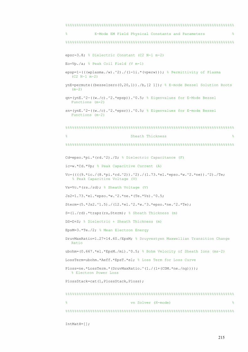
215

%%%%%%%%%%%%%%%%%%%%%%%%%%%%%%%%%%%%%%%%%%%%%%%%%%%%%%%%%%%%%%%%%%%%%%%%%%%

% E-Mode EM Field Physical Constants and Parameters %

%%%%%%%%%%%%%%%%%%%%%%%%%%%%%%%%%%%%%%%%%%%%%%%%%%%%%%%%%%%%%%%%%%%%%%%%%%%

epsr=3.8; % Dielectric Constant (C2 N-1 m-2)

Eo=Vp./a; % Peak Coil Field (V m-1)

epsp=1-(((wplasma./w).^2)./(1-1i.*(vperw))); % Permittivity of Plasma

(C2 N-1 m-2)

ynE=permute((besselzero(0,20,1))./b,[2 1]); % E-mode Bessel Solution Roots

(m-2)

qn=(ynE.^2-((w./c).^2.*epsp)).^0.5; % Eigenvalues for E-Mode Bessel

Functions (m-2)

sn=(ynE.^2-((w./c).^2.*epsr)).^0.5; % Eigenvalues for E-mode Bessel

Functions (m-2)

%%%%%%%%%%%%%%%%%%%%%%%%%%%%%%%%%%%%%%%%%%%%%%%%%%%%%%%%%%%%%%%%%%%%%%%%%%%

% Sheath Thickness %

%%%%%%%%%%%%%%%%%%%%%%%%%%%%%%%%%%%%%%%%%%%%%%%%%%%%%%%%%%%%%%%%%%%%%%%%%%%

Cd=epso.*pi.*(rd.^2)./D; % Dielectric Capacitance (F)

ic=w.*Cd.*Vp; % Peak Capacitive Current (A)

Vc=((((9.*ic./(8.*pi.*rd.^2)).^2)./(1.73.*el.*epso.*w.^2.*ne)).^2)./Te;

% Peak Capacitive Voltage (V)

Vs=Vc.*(rs./rd); % Sheath Voltage (V)

Js2=1.73.*el.*epso.*w.^2.*ne.*(Te.*Vs).^0.5;

Sterm=(5.*Js2.^1.5)./(12.*el.^2.*w.^3.*epso.*ne.^2.*Te);

S=(1./rd).*trapz(rs,Sterm); % Sheath Thickness (m)

DS=D+S; % Dielectric + Sheath Thickness (m)

EpsM=3.*Te./2; % Mean Electron Energy

DruvMaxRatio=1.27+14.60./EpsM; % Druyvestyen Maxwellian Transition Change

Ratio

ubohm=(0.667.*el.*EpsM./mi).^0.5; % Bohm Velocity of Sheath Ions (ms-2)

LossTerm=ubohm.*Aeff.*EpsT.*el; % Loss Term for Loss Curve

Ploss=ne.*LossTerm.*(DruvMaxRatio.^(1./(1+(CDM.*ne./ng))));

% Electron Power Loss

PlossStack=cat(1,PlossStack,Ploss);

%%%%%%%%%%%%%%%%%%%%%%%%%%%%%%%%%%%%%%%%%%%%%%%%%%%%%%%%%%%%%%%%%%%%%%%%%%%

% vn Solver (H-mode) %

%%%%%%%%%%%%%%%%%%%%%%%%%%%%%%%%%%%%%%%%%%%%%%%%%%%%%%%%%%%%%%%%%%%%%%%%%%%

IntMatH=[];

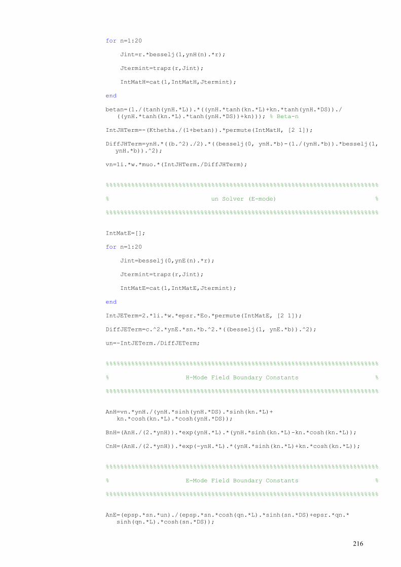
216

for n=1:20

Jint=r.*besselj(1,ynH(n).*r);

Jtermint=trapz(r,Jint);

IntMatH=cat(1,IntMatH,Jtermint);

end

betan=(1./(tanh(ynH.*L)).*((ynH.*tanh(kn.*L)+kn.*tanh(ynH.*DS))./

((ynH.*tanh(kn.*L).*tanh(ynH.*DS))+kn))); % Beta-n

IntJHTerm=-(Kthetha./(1+betan)).*permute(IntMatH, [2 1]);

DiffJHTerm=ynH.*((b.^2)./2).*((besselj(0, ynH.*b)-(1./(ynH.*b)).*besselj(1,

ynH.*b)).^2);

vn=1i.*w.*muo.*(IntJHTerm./DiffJHTerm);

%%%%%%%%%%%%%%%%%%%%%%%%%%%%%%%%%%%%%%%%%%%%%%%%%%%%%%%%%%%%%%%%%%%%%%%%%%%

% un Solver (E-mode) %

%%%%%%%%%%%%%%%%%%%%%%%%%%%%%%%%%%%%%%%%%%%%%%%%%%%%%%%%%%%%%%%%%%%%%%%%%%%

IntMatE=[];

for n=1:20

Jint=besselj(0,ynE(n).*r);

Jtermint=trapz(r,Jint);

IntMatE=cat(1,IntMatE,Jtermint);

end

IntJETerm=2.*1i.*w.*epsr.*Eo.*permute(IntMatE, [2 1]);

DiffJETerm=c.^2.*ynE.*sn.*b.^2.*((besselj(1, ynE.*b)).^2);

un=-IntJETerm./DiffJETerm;

%%%%%%%%%%%%%%%%%%%%%%%%%%%%%%%%%%%%%%%%%%%%%%%%%%%%%%%%%%%%%%%%%%%%%%%%%%%

% H-Mode Field Boundary Constants %

%%%%%%%%%%%%%%%%%%%%%%%%%%%%%%%%%%%%%%%%%%%%%%%%%%%%%%%%%%%%%%%%%%%%%%%%%%%

AnH=vn.*ynH./(ynH.*sinh(ynH.*DS).*sinh(kn.*L)+

kn.*cosh(kn.*L).*cosh(ynH.*DS));

BnH=(AnH./(2.*ynH)).*exp(ynH.*L).*(ynH.*sinh(kn.*L)-kn.*cosh(kn.*L));

CnH=(AnH./(2.*ynH)).*exp(-ynH.*L).*(ynH.*sinh(kn.*L)+kn.*cosh(kn.*L));

%%%%%%%%%%%%%%%%%%%%%%%%%%%%%%%%%%%%%%%%%%%%%%%%%%%%%%%%%%%%%%%%%%%%%%%%%%%

% E-Mode Field Boundary Constants %

%%%%%%%%%%%%%%%%%%%%%%%%%%%%%%%%%%%%%%%%%%%%%%%%%%%%%%%%%%%%%%%%%%%%%%%%%%%

AnE=(epsp.*sn.*un)./(epsp.*sn.*cosh(qn.*L).*sinh(sn.*DS)+epsr.*qn.*

sinh(qn.*L).*cosh(sn.*DS));

217

CnE=(AnE./(2.*epsp.*sn)).*exp(-sn.*L).*(epsp.*sn.*cosh(qn.*L)+

epsr.*qn.*sinh(qn.*L));

DnE=(AnE./(2.*epsp.*sn)).*exp(sn.*L).*(epsp.*sn.*cosh(qn.*L)-epsr.*qn.*

sinh(qn.*L));

%%%%%%%%%%%%%%%%%%%%%%%%%%%%%%%%%%%%%%%%%%%%%%%%%%%%%%%%%%%%%%%%%%%%%%%%%%%

% H-Mode Power Iteration Loop %

%%%%%%%%%%%%%%%%%%%%%%%%%%%%%%%%%%%%%%%%%%%%%%%%%%%%%%%%%%%%%%%%%%%%%%%%%%%

Ethethar=[];

for n=1:rlim

Ethethasum=sum((BnH.*exp(-ynH.*(L+D+S))+CnH.*exp(ynH.*(L+D+S))).*

besselj(1,ynH.*r(n)));

Ethethar=cat(2,Ethethar,Ethethasum);

end

Ethetha=Ethethar;

PHMode=-pi.*Kthetha.*trapz(r,r.*Ethetha); % Absorbed H-mode Power (W)

PHModeAbs=abs(PHMode); % Absolute Absorbed H-mode Power (W)

PHModeReal=real(PHMode); % Real Component of Absorbed H-mode Power (W)

if isnan(PHModeReal)==1

PHModeReal=0;

else

end

PHMStack=cat(1,PHMStack,PHModeReal);

%%%%%%%%%%%%%%%%%%%%%%%%%%%%%%%%%%%%%%%%%%%%%%%%%%%%%%%%%%%%%%%%%%%%%%%%%%%

% E-Mode Power Iteration Loop %

%%%%%%%%%%%%%%%%%%%%%%%%%%%%%%%%%%%%%%%%%%%%%%%%%%%%%%%%%%%%%%%%%%%%%%%%%%%

Bthethar=[];

for n=1:rlim

Bthethasum=sum((CnE.*exp(sn.*(L+D+S))+DnE.*exp(-sn.*(L+D+S))).*

besselj(1,ynE.*r(n)));

Bthethar=cat(2,Bthethar,Bthethasum);

end

Bthetha=Bthethar;

Eradiusr=[];

for n=1:rlim

Eradiussum=((1i.*c.^2)./(w.*epsr)).*sum(sn.*(CnE.*exp(sn.*(L+D+S))-

DnE.*exp(-sn.*(L+D+S))).*besselj(1,ynE.*r(n)));

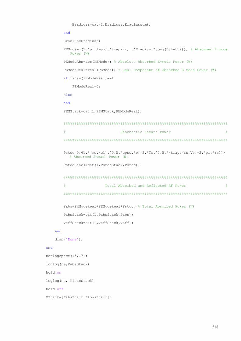
218

Eradiusr=cat(2,Eradiusr,Eradiussum);

end

Eradius=Eradiusr;

PEMode=-(2.*pi./muo).*trapz(r,r.*Eradius.*conj(Bthetha)); % Absorbed E-mode

Power (W)

PEModeAbs=abs(PEMode); % Absolute Absorbed E-mode Power (W)

PEModeReal=real(PEMode); % Real Component of Absorbed E-mode Power (W)

if isnan(PEModeReal)==1

PEModeReal=0;

else

end

PEMStack=cat(1,PEMStack,PEModeReal);

%%%%%%%%%%%%%%%%%%%%%%%%%%%%%%%%%%%%%%%%%%%%%%%%%%%%%%%%%%%%%%%%%%%%%%%%%%%

% Stochastic Sheath Power %

%%%%%%%%%%%%%%%%%%%%%%%%%%%%%%%%%%%%%%%%%%%%%%%%%%%%%%%%%%%%%%%%%%%%%%%%%%%

Pstoc=0.61.*(me./el).^0.5.*epso.*w.^2.*Te.^0.5.*(trapz(rs,Vs.*2.*pi.*rs));

% Absorbed Sheath Power (W)

PstocStack=cat(1,PstocStack,Pstoc);

%%%%%%%%%%%%%%%%%%%%%%%%%%%%%%%%%%%%%%%%%%%%%%%%%%%%%%%%%%%%%%%%%%%%%%%%%%%

% Total Absorbed and Reflected RF Power %

%%%%%%%%%%%%%%%%%%%%%%%%%%%%%%%%%%%%%%%%%%%%%%%%%%%%%%%%%%%%%%%%%%%%%%%%%%%

Pabs=PHModeReal+PEModeReal+Pstoc; % Total Absorbed Power (W)

PabsStack=cat(1,PabsStack,Pabs);

veffStack=cat(1,veffStack,veff);

end

disp('Done');

end

ne=logspace(15,17);

loglog(ne,PabsStack)

hold on

loglog(ne, PlossStack)

hold off

PStack=[PabsStack PlossStack];

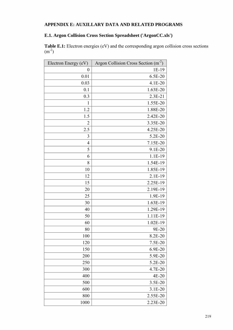
219

APPENDIX E: AUXILLARY DATA AND RELATED PROGRAMS

E.1. Argon Collision Cross Section Spreadsheet ('ArgonCC.xls')

Table E.1: Electron energies (eV) and the corresponding argon collision cross sections (m-2)

Electron Energy (eV) Argon Collision Cross Section (m-2) 0 1E-19

0.01 6.5E-20 0.03 4.1E-20 0.1 1.63E-20 0.3 2.3E-21

1 1.55E-20 1.2 1.88E-20 1.5 2.42E-20

2 3.35E-20 2.5 4.25E-20

3 5.2E-20 4 7.15E-20 5 9.1E-20 6 1.1E-19 8 1.54E-19

10 1.85E-19 12 2.1E-19 15 2.25E-19 20 2.19E-19 25 1.9E-19 30 1.63E-19 40 1.29E-19 50 1.11E-19 60 1.02E-19 80 9E-20

100 8.2E-20 120 7.5E-20 150 6.9E-20 200 5.9E-20 250 5.2E-20 300 4.7E-20 400 4E-20 500 3.5E-20 600 3.1E-20 800 2.55E-20

1000 2.23E-20

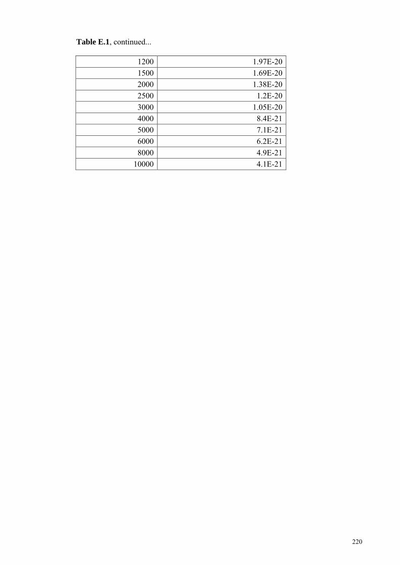
220

Table E.1, continued...

1200 1.97E-20 1500 1.69E-20 2000 1.38E-20 2500 1.2E-20 3000 1.05E-20 4000 8.4E-21 5000 7.1E-21 6000 6.2E-21 8000 4.9E-21

10000 4.1E-21

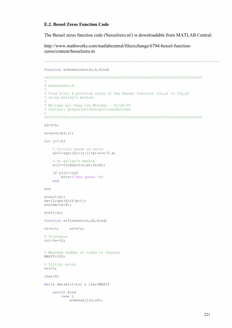
221

E.2. Bessel Zeros Function Code

The Bessel zeros function code ('besselzero.m') is downloadable from MATLAB Central: http://www.mathworks.com/matlabcentral/fileexchange/6794-bessel-function-zeros/content/besselzero.m ---------------------------------------------------------------------------

function x=besselzero(n,k,kind)

%%%%%%%%%%%%%%%%%%%%%%%%%%%%%%%%%%%%%%%%%%%%%%%%%%%%%%%%%%%%%%%%%%%%%%%%%%%

%

% besselzero.m

%

% Find first k positive zeros of the Bessel function J(n,x) or Y(n,x)

% using Halley's method.

%

% Written by: Greg von Winckel - 01/25/05

% Contact: gregvw(at)chtm(dot)unm(dot)edu

%

%%%%%%%%%%%%%%%%%%%%%%%%%%%%%%%%%%%%%%%%%%%%%%%%%%%%%%%%%%%%%%%%%%%%%%%%%%%

k3=3*k;

x=zeros(k3,1);

for j=1:k3

% Initial guess of zeros

x0=1+sqrt(2)+(j-1)*pi+n+n^0.4;

% Do Halley's method

x(j)=findzero(n,x0,kind);

if x(j)==inf

error('Bad guess.');

end

end

x=sort(x);

dx=[1;abs(diff(x))];

x=x(dx>1e-8);

x=x(1:k);

function x=findzero(n,x0,kind)

n1=n+1; n2=n*n;

% Tolerance

tol=1e-12;

% Maximum number of times to iterate

MAXIT=100;

% Initial error

err=1;

iter=0;

while abs(err)>tol & iter<MAXIT

switch kind

case 1

a=besselj(n,x0);

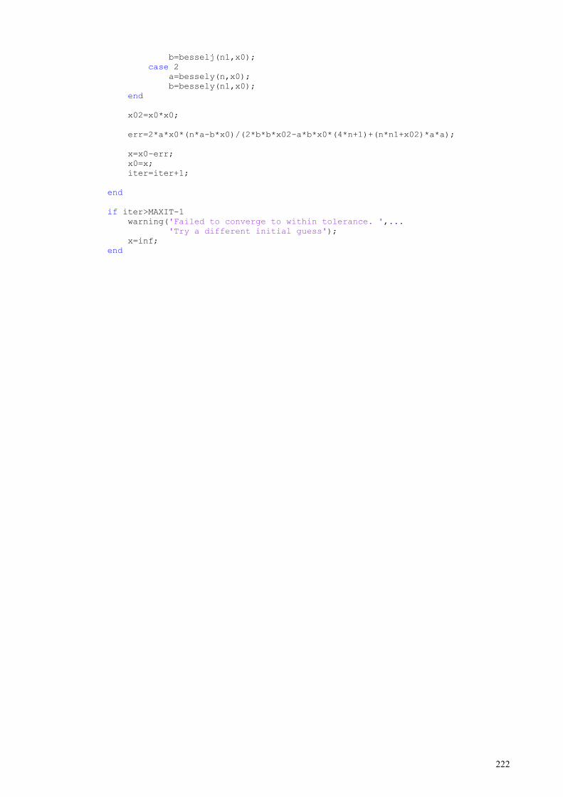
222

b=besselj(n1,x0);

case 2

a=bessely(n,x0);

b=bessely(n1,x0);

end

x02=x0*x0;

err=2*a*x0*(n*a-b*x0)/(2*b*b*x02-a*b*x0*(4*n+1)+(n*n1+x02)*a*a);

x=x0-err;

x0=x;

iter=iter+1;

end

if iter>MAXIT-1

warning('Failed to converge to within tolerance. ',...

'Try a different initial guess');

x=inf;

end

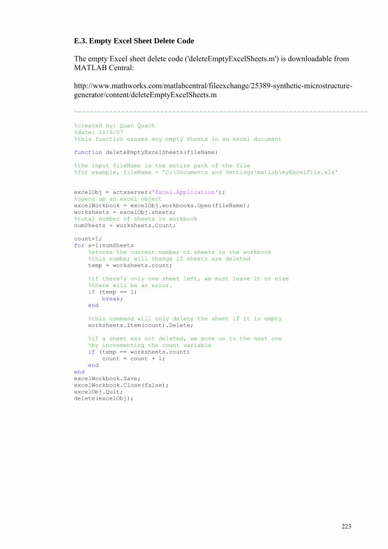
223

E.3. Empty Excel Sheet Delete Code

The empty Excel sheet delete code ('deleteEmptyExcelSheets.m') is downloadable from MATLAB Central: http://www.mathworks.com/matlabcentral/fileexchange/25389-synthetic-microstructure-generator/content/deleteEmptyExcelSheets.m --------------------------------------------------------------------------- %created by: Quan Quach

%date: 11/6/07

%this function erases any empty sheets in an excel document

function deleteEmptyExcelSheets(fileName)

%the input fileName is the entire path of the file

%for example, fileName = 'C:\Documents and Settings\matlab\myExcelFile.xls'

excelObj = actxserver('Excel.Application');

%opens up an excel object

excelWorkbook = excelObj.workbooks.Open(fileName);

worksheets = excelObj.sheets;

%total number of sheets in workbook

numSheets = worksheets.Count;

count=1;

for x=1:numSheets

%stores the current number of sheets in the workbook

%this number will change if sheets are deleted

temp = worksheets.count;

%if there's only one sheet left, we must leave it or else

%there will be an error.

if (temp == 1)

break;

end

%this command will only delete the sheet if it is empty

worksheets.Item(count).Delete;

%if a sheet was not deleted, we move on to the next one

%by incrementing the count variable

if (temp == worksheets.count)

count = count + 1;

end

end

excelWorkbook.Save;

excelWorkbook.Close(false);

excelObj.Quit;

delete(excelObj);

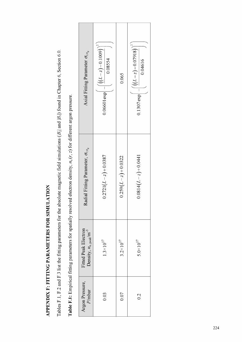
224

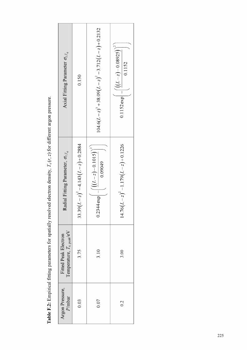
225

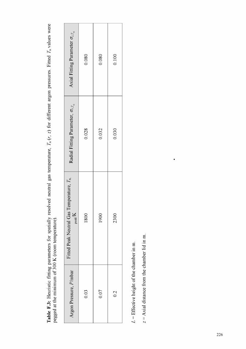
226