study of the pedestal dynamics and stability during the elm cycle a. burckhart advisor: dr. e....

Study of the pedestal dynamics andstability during the ELM cycle

A. Burckhart

Advisor: Dr. E. WolfrumAcademic advisor: Prof. Dr. H. Zohm

MPI für Plasmaphysik, EURATOM Association

A. Burckhart, PhD network, September 30th, 2010

A. Burckhart, PhD network, September 30th, 2010 2/30

• Motivation: why study ELMs?

• Overview on peeling ballooning theory and ELMs

• Evolution of Te, ne and pe during the ELM cycle

• Stability calculations

• Conclusions

Overview






• Conclusions

Overview


Motivation

• Highest performance is found in H-mode plasmas featuring type-I ELMs Forseen operation scenario for ITER

• Edge localized modes (ELMs) are instabilities of the plasma edge, leading to a periodic deterioration of the pedestal profiles

• They cause massive power loads on the divertor, up to 10% of the confined energy in less than 1ms

• They cause high energy and particle losses

• They “clean” the plasma by expelling impurities

•They are not yet fully understood• Investigating the dynamic behavior of pedestal profiles can lead to a better

understanding of ELMs, and maybe ultimately to their control

• Stability calculations are usually performed for one time point directly before the ELM crash, what about the temporal evolution of the stability?






• Conclusions

Overview


Plasma stability

• We consider a plama equilibrium with the total potential energy W, and calculate the effect of an arbitrary small displacement ξ

• If δW > 0, the system is stable, with δW < 0 it is unstable

ξ

ξ

stable (oszillation) unstable

δW < 0δW > 0


,1||0

2

0

2

0

20

0

,1

0

2

1

2

22

1

2

1

Bb

B

Br

jp

pB

W

dW

WWW

plasma

plasma

vac

vacuum

vacuumplasma

Instability: The change of potential energy is negative

Stability code: Find that minimises W

Field line bending

Compression of magnetic field lines

Plasma compression

Pressure driven modes

Current driven modes

Stabilising:

Destabilising:

(vacuum field line bending, always stabilising)

Edge stability

[Saarelma, JET 13.09.2010]


• Current driven instabilities that are localized radially at the plasma edge and poloidally near the X-point.

• Usually low-n

n=7

Mode localized near the x-points.


Peeling modes


• Driven by the pressure gradient.

• localized on the low field side.

• Radially more extended than peeling modes.

• Usually high-n.

n=20

Mode localized at the bad curvature region


Edge ballooning modes


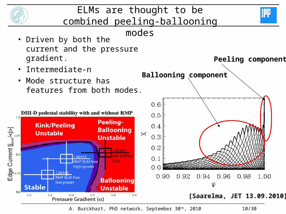
• Driven by both the current and the pressure gradient.

• Intermediate-n• Mode structure has

features from both modes.

Peeling component

Ballooning component


ELMs are thought to be combined peeling-ballooning modes


ELMs expel particles from the plasma

[T. Lunt]

• Glow: mostly H-alpha, cold and dense

• Filaments expelled, travelling along field lines

• Highest intensity lasts less than 1ms


Te and ne pedestals relax due to ELMs

• Ipolsola: currents in the divertor, used as ELM indicator

• Te relaxes quickly during ELM crash, then slowly recovers

• ne also relaxes, but evolves around „pivot point“: ne inside drops, ne in the SOL increases






• Conclusions

Overview


Te recovery shows several distinct phases

during ELMTe is small

initial recoveryof Te

Te recoverystalls Te recovery

continues

Te exhibitslarge fluctuations

Max(Te) mapped relative to t=0


Only one short recovery phase ~ 2-3ms

ne recovers differently than Te

Overshoot at the end of the recovery

Last phase is stationary,but large scale fluctuations

Te pedestal takes around 7ms to fully recover, ne pedestal only 4ms


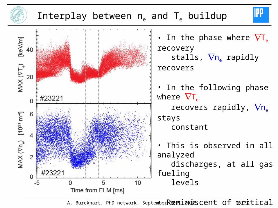
Interplay between ne and Te buildup

• In the phase where Te recovery stalls, ne rapidly recovers

• In the following phase where Te recovers rapidly, ne stays constant

• This is observed in all analyzed discharges, at all gas fueling levels

• Reminiscent of critical value of e=Ln/LT above which Te is clamped: possibly ETGs are responsible for pause in the recovery of the Te profile


New laser triggering method will allow for ahigher density of TS data points

• Next steps:

• Improve characterization of edge Te profile recovery using TS data, which does not have the shine through problem (no accurate ECE data outside

ρpol=0.995 ) long discharges necessary

• Thomson scattering diagnostic:• Six 20Hz Nd-Yag lasers One profile every 8.3ms• Or: burst mode, fire all lasers in a given time interval

• Next campaign:

ELM detectedby XVR

DelayA + n*x

optical signal triggers laser

Result:All data points from the TS system lie in time interval of the ELM cycle that we want to analyze

TS data point


Next steps concerning pedestal dynamics

• Test reproducibility of interplay between Te and ne in the recovery of the pedestal profiles on other devices, starting with JET

• Very good Thomson scattering profiles available, but only 20Hz long discharges and coherent data selection necessary

• Fast ECE data available, but low resolution in the pedestal region, and shine through effect often more pronounced than on AUG

• Reflectometry measurements, Li-beam and DCN also available but not suited for calculating gradients and/or temporal resolution not sufficient

• No method that combines the data from different diagnostics to one joint profile (c.f. integrated data analysis at AUG)

• Start with analyzing TS and ECE data of „old“ discharges

• Then analyze dependencies of the pedestal dynamics on collisionality and on fueling level


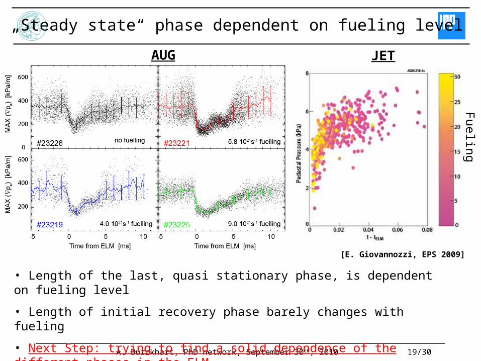
AUG

• Length of the last, quasi stationary phase, is dependent on fueling level

• Length of initial recovery phase barely changes with fueling

• Next Step: trying to find a solid dependence of the different phases in the ELM cycle on the fueling level (AUG and JET)

„Steady state“ phase dependent on fueling level

JET

Fueling

[E. Giovannozzi, EPS 2009]


Reaching the pe limit does not necessarily lead to an ELM

• Clearly, a limit to max(pe) exists, but reaching it does not automatically trigger an ELM

• Some ELMs seem to be triggered by reaching max(pe) (consistent with JETTO simulation [J. Lönnroth, PPCF 2004])

• Others can sit at the pressure limit for several ms before ELM happens (seen before on AUG [T. Kass, NF 1998] and DIII-D, [R. Groebner, NF 2009])

‚fast‘ ELM frequency ‚slow‘ ELM frequency


Current diffusion cannot explain delayed ELM

peeling boundary

ballo

on

ing

bo

un

dary

[J. Connor, Phys.Plasmas 1998]

• ELM thought to be driven by combination of pressure and current gradient• Pressure gradient limited by ballooning mode• Edge current gradient limited by peeling (=very edge localized kink) mode

• Bootstrap current roughly proportional to pe, but delayed by about 1ms because of current diffusion cannot explain 6-7ms observed between reaching final pe and occurrence of the next ELM


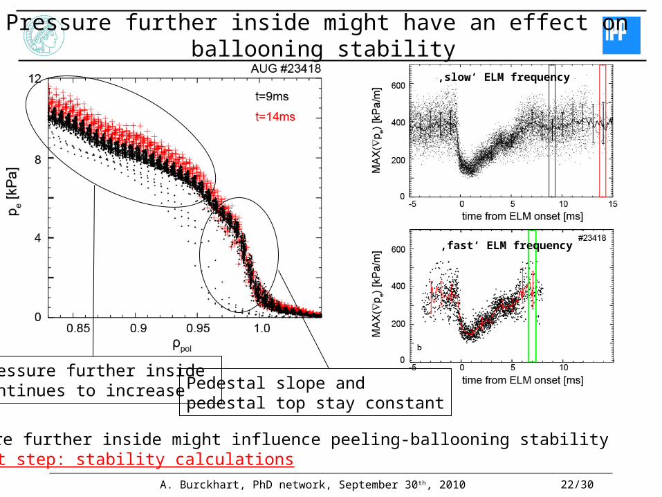
Pressure further inside continues to increase

• Pressure further inside might influence peeling-ballooning stability• Next step: stability calculations

Pressure further inside might have an effect on ballooning stability

Pedestal slope and pedestal top stay constant

‚fast‘ ELM frequency

‚slow‘ ELM frequency






• Conclusions

Overview


ELM-coherent averaged profiles

and magnetic data

CLISTE equilibrium (with kinetic

profiles)

ILSA stability

calculations

Stability calculations performed in several steps

HELENA High resolution

equilibrium


Experimental data is ELM synchronized

ne (1019 m-3)

Te (eV)

[M. Dunne]


and magnetic data


profiles)

ILSA stability

calculations


equilibrium


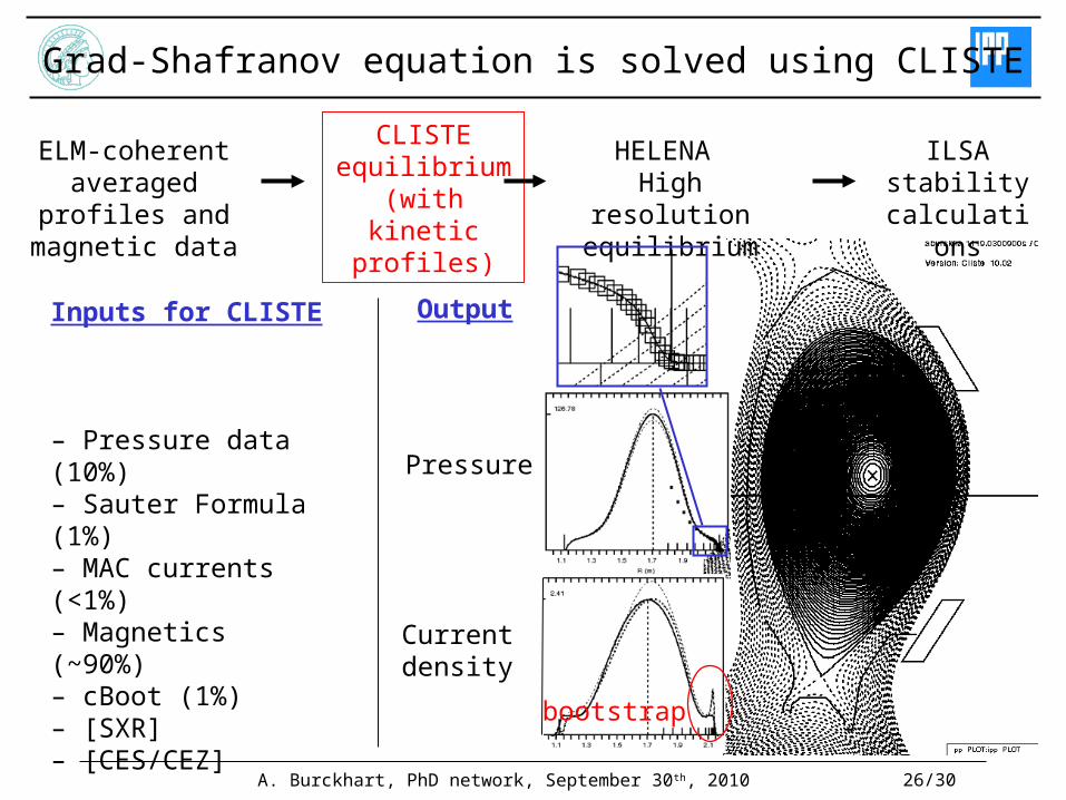
Grad-Shafranov equation is solved using CLISTE

Inputs for CLISTE

– Pressure data (10%)– Sauter Formula (1%)– MAC currents (<1%)– Magnetics (~90%)– cBoot (1%)– [SXR]– [CES/CEZ] Current

density

bootstrap

Pressure


and magnetic data


profiles)

ILSA stability

calculations


equilibrium

Output


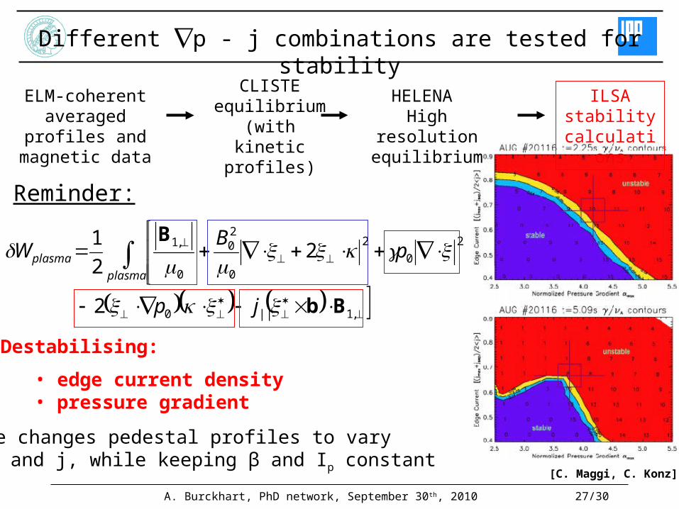
Different p - j combinations are tested for stability

[C. Maggi, C. Konz]

,1||0

2

0

2

0

20

0

,1

2

22

1

Bb

B

jp

pB

Wplasma

plasma

Destabilising:

• edge current density• pressure gradient

Reminder:


and magnetic data


profiles)

ILSA stability

calculations


equilibrium

Code changes pedestal profiles to vary p and j, while keeping β and Ip constant


•First calculations would suggest a pedestal far away from stability limit, but:

•CLISTE output had too low gradients•Need to run CLISTE and ILSA again, carefully comparing CLISTE results with experimental data

First stability calculations performed, but need to be repeated

[C. Konz]






• Conclusions

Overview


Conclusions and to-do’s

Study of ELM cycle with high temporal and spatial resolution sheds new light on both transport and stability of the pedestal

• Interplay between recovery of Te and ne observed on all analyzed AUG discharges, still to be studied on JET

• Better characterization of Te recovery might be possible with TS (no ECE shine through)

• Maximum of pe and jb can be reached well before ELM onset

• While peeling ballooning model is consistent with limits to pedestal pressure, there is still a physics ingredient missing to explain the ELM trigger

- Influence from pressure further inside to be assessed

- Temporal evolution of the stability to be characterized, comparison between stability of slow and fast ELM-cycles

study of the pedestal dynamics and stability during the elm cycle a. burckhart advisor: dr. e....

Documents

phd network

plasma stability

study elms

peeling modes

elms evolution of t

edge ballooning modes

burckhart advisor

iter edge localized