study of wave propagation and potential structures …
TRANSCRIPT

STUDY OF WAVE PROPAGATION AND POTENTIAL
STRUCTURES IN AN EXPANDING HELICON PLASMA
By
KSHITISH KUMAR BARADA
PHYS06200704009
Institute for Plasma Research, Gandhinagar
A thesis submitted to the
Board of Studies in Physical Sciences
In partial fulfillment of requirements
For the Degree of
DOCTOR OF PHILOSOPHY
Of
HOMI BHABHA NATIONAL INSTITUTE
August, 2013


“There is nothing in a caterpillar that tells you it's going to be a butterfly”
……… Richard Buckminster Fuller
Architect, systems theorist, author, designer, inventor, and futurist

Dedicated to
My Family

ACKNOWLEDGEMENT
This thesis is complete because of numerous supports I have got from different people. First and
foremost I thank my supervisor Dr. Prabal Kumar Chattopadhyay for his guidance and support
throughout this thesis work. Though I have done experiments in my university, he introduced me
to experimental techniques through the study of electrical noise. I would like to thank him for the
freedom and openness he provided me with. Discussions with him always started from
experimental techniques and ended in nice physics. I would also like to thank Dr. Joydeep Ghosh
for encouragement in the rough periods of my thesis and also for fruitful physics discussions.
Thanks are due to Prof. Yogesh Saxena for constant encouragement and constructive criticism
which gave favorable direction to this thesis. I would also like thank Dr. Devendra Sharma for
the understanding I have on sheaths and double layers.
I am indebted to Dr. R. Ganesh, Dr. Sudip Sengupta, Dr. Devendra Sharma, Prof. R. Jha and
Prof. Amita Das for excellent teaching during the course work which helped me to understand
basics of plasma physics. I express my sincere thanks to Academic Dean, Dr. Mukherjee for his
timely help. I would like to extend my sincere gratitude to Shravan bhai, Shilpa mam, Smita
mam, Pragnya mam, Arundhati mam, Hemant bhai, Shailendra bhai, Sutapa mam and all Library
and Computer Centre Staff members for their support on many occasions. I extend my thanks to
Atrey Sir, Chamunde ji, Harvey ji, Sourbhan ji, Khanduri ji, Vartak ji, Savai ji, Sirin mam, Silel
ji and Hitesh bhai for all the administrative helps.
Staying in a hostel away from home never turned out to be difficult because of my friends,
juniors and seniors with whom I discussed my life, my Physics problems. Playing in the
weekends was utmost a necessity in these seven years. I would like thank every one of them for
their love and support they have provided me with during this period. I thank you Ujjwal,
Gurudatt, Vikram, Sita, Prabal, Ashwin, Deepak for always reminding me that we are the best. I
thank Neeraj bheya, Pintuda, Ritudi, Rajneesh bheya, Manas bheya, Bhaskar bheya, Anuraga
bheya, Mayadi, Kishor bheya, Vikrant bheya, Sunitadi, Shekhar bhai, Jugal bhai, Satya bhai,
Sharad bhai, Sushil, Rameswar, Sanat, Pravesh, Manjeet, Sayak, Soumen, Aditya, Vara, Mangi,

Vidhi, Deepa, Akanksha, Neeraj, Chandrasekhar, Meghraj, Harish, Rupendra, Bibhu, Samir,
Arghya, Debu, Bhumika, Anup, Ratan, Amit, Sonu, Umesh, Surabhi and Modhu.
I cannot forget those relaxing moments while trekking in the forests of Gujarat with Govind bhai,
Mahesh and Ghate in the frustrating periods of my life in between. Surprisingly, it was awesome
to know you three and I hope I have made a lasting impression on you as you have on me. In the
lab Sayak, Manjit and Soumen always provided a conducive and joyful atmosphere for physics
study. Thank you friends. Arindam bheya, it’s you who triggered the interest in diagnostics in
me. What a time we had! Thank you very much for being a part of my life even today. I would
like to thank Acharya ji, Sadrakhiya ji, Vishnu bhai, Swadesh bhai, Narendra bhai, Madan ji and
Variaji for their support in building up my experimental set up and Madan ji for showing the
Ahmedabad market. Thanks are due to Jignesh bhai, Praveenlal and all electronics group
member for their help in electronics circuits for diagnostics. Jiba’s food has always been blended
with his love for us which made the hygienic and healthy food tastier. When I used to go home, I
always missed his food.
This work would not have completed without the constant support, patience and encouragement
from my parents and family members. Dear Daddy, I learnt honesty from you and Mummy, I
learnt determination from you. My sweet younger sisters and brother, your love will remain
always with me. Finally, I would like to thank all those who have come into my life, putting an
unforgettable impression in my life including my classmates and teachers at school, college and
University.
Kshitish Kumar Barada
LIST OF PUBLICATIONS
1. Kshitish K. Barada, P. K. Chattopadhyay, J. Ghosh, Sunil Kumar, and Y. C. Saxena.
“A linear helicon plasma device with controllable magnetic field gradient.” Review of
Scientific Instruments 83, 063501 (2012).
2. Kshitish K. Barada, P. K. Chattopadhyay, J. Ghosh, Sunil Kumar, and Y. C. Saxena.
“Observation of low magnetic field density peaks.” Under review Physics of Plasmas
20, 042119 (2013)
3. Kshitish K. Barada, P. K. Chattopadhyay, J. Ghosh, Sunil Kumar, and Y. C. Saxena.
"Experimental Observation of Left Polarized Wave Absorption near Electron Cyclotron
Resonance Frequency in Helicon Antenna Produced Plasma." Physics of Plasmas 20,
012123(2013)
4. Kshitish K. Barada, P. K. Chattopadhyay, J. Ghosh, D.Sharma, and Y. C. Saxena.
“Charging of a plasma filled dielectric glass wall wrapped in a helicon antenna” to be
submitted.
5. Kshitish K. Barada, P. K. Chattopadhyay, J. Ghosh, D. Sharma, and Y. C. Saxena.
“Diverging magnetic field near helicon antenna increases antenna coupling efficiency in
low magnetic field operation.” To be submitted.
6. Kshitish K. Barada, P. K. Chattopadhyay, J. Ghosh, D. Sharma, and Y. C. Saxena.
“Transition from a quasi double layer to a multiple double layer containing current free
plasma” to be submitted.
7. Kshitish K. Barada, P. K. Chattopadhyay, J. Ghosh, D. Sharma, and Y. C. Saxena. “The
downstream density peak in low magnetic field helicon discharge” to be submitted.
i
Contents Abstract…………………………………………………………………………………………. iv
List of Figures…………………………………………………………………………………… v
List of Tables…………………………………………………………………………………….xi
Chapter 1: Introduction
1.1 History of Helicon Sources ....................................................................................................... 1
1.2 Review of Relevant Previous Work .......................................................................................... 3
1.3 Motivation and objective .......................................................................................................... 6
1.4 Description of chapters and main findings ............................................................................... 7
References ..................................................................................................................................... 11
Chapter 2: Helicon Physics
2.1 Introduction ............................................................................................................................. 16
2.2 Derivation of dispersion relation ............................................................................................ 17
2.2.1 Vacuum Waves ................................................................................................................ 17
2.2.2 Plasma Waves .................................................................................................................. 20
2.3 Oblique propagation and Resonance cone .............................................................................. 32
2.4 Helicon waves in a cylinder .................................................................................................... 34
2.5 Helicon mode structure in non uniform radial density ........................................................... 37
2.6 Models of Helicon Power Deposition ..................................................................................... 38
2.7 Mode Transitions in Helicon Discharge ................................................................................. 39
2.8 Summary of the Chapter ......................................................................................................... 41
References ..................................................................................................................................... 42
Chapter 3: Experimental Set up and Diagnostics
3.1 Introduction ............................................................................................................................. 45

ii
3.2 Vacuum Vessel and Vacuum System ..................................................................................... 45
3.3 Electromagnets ........................................................................................................................ 47
3.4 Antenna and RF Matching Circuit .......................................................................................... 49
3.4.1 The Antenna ..................................................................................................................... 51
3.4.2 Matching Network............................................................................................................ 52
3.5 Diagnostics .............................................................................................................................. 56
3.5.1 Single Langmuir Probe..................................................................................................... 56
3.5.2 Wall Probe ........................................................................................................................ 65
3.5.3 RF Compensated Probe .................................................................................................... 68
3.5.4 Double Langmuir Probe ................................................................................................... 73
3.5.5 Triple Langmuir Probe ..................................................................................................... 77
3.5.6 Emissive Probe ................................................................................................................. 82
3.5.7 B-dot Probe ...................................................................................................................... 90
3.5.8 Antenna-Plasma Load Measurements .............................................................................. 92
3.6 Summary of Chapter 3 ............................................................................................................ 93
References ..................................................................................................................................... 94
Chapter 4: Helicon Characterization
4.1 Antenna Efficiency ................................................................................................................. 98
4.2 Discharge mode transitions ................................................................................................... 101
4.3 Mode structure at Low magnetic field .................................................................................. 104
4.4 Axial density profile ............................................................................................................. 107
4.5 Observation of Current free double layer ............................................................................. 109
4.6 Summary of Chapter 4 .......................................................................................................... 110
References ................................................................................................................................... 112
Chapter 5: Low Magnetic Field Helicon Study

iii
5.1 Introduction ........................................................................................................................... 114
5.2 Multiple Density Peaks ......................................................................................................... 117
5.3 Polarization reversal and asymmetric density peaking ......................................................... 126
5.4 Downstream Density Peak .................................................................................................... 134
5.5 Efficient Low Field Helicon Source ..................................................................................... 139
5.6 Conclusions ........................................................................................................................... 144
References ............................................................................................................................... 146
Chapter 6: Current Free Double Layer
6.1 Introduction ........................................................................................................................... 149
6.2 Boltzmann Plasma Expansion............................................................................................... 150
6.3 Double Layer ........................................................................................................................ 152
6.4 Current Free Double layer .................................................................................................... 155
6.4.1 Helicon CFDL experiments ........................................................................................... 155
6.4.2 Helicon CFDL Models ................................................................................................... 156
6.4.3 Helicon CFDL instabilities ............................................................................................ 158
6.4.4 Effect of Magnetic field Strength and Gradient ............................................................. 159
6.5 Study of Dielectric Wall Charging ....................................................................................... 160
6.6 Experimental Observations of multiple CFDL ..................................................................... 165
6.7 Summary of Chapter 6 .......................................................................................................... 174
References ................................................................................................................................... 175
Chapter 7: Conclusion and Future Work
7.1 Conclusion ............................................................................................................................ 179
7.2 Future Work .......................................................................................................................... 181

iv
ABSTRACT
Diverging magnetic fields are found naturally in universe including our magnetosphere
and in solar coronal funnels. Diverging magnetic fields are used in expanding plasmas to
accelerate particles by electric fields produced by localized potential structures, called
double layer, formed self consistently inside the plasma. Acceleration of charged particles
in low temperature plasmas is of interest to surface function modification as well as to
development of electrostatic thrusters. This thesis devotes its study to find the role of
diverging magnetic fields in helicon source operation and self consistent potential
structure formation in bulk of plasma. A geometrically expanding (small diameter source
attached to a bigger diameter expansion chamber) linear helicon device along with various
diagnostics is designed and built with a diverging magnetic field. The helicon plasma
produced with an m = +1 half helical antenna powered by a 2.5 kW RF power source at
13.56 MHz is characterized. Mode transitions are observed and mode structures are
studied at low magnetic fields (<100 G). Though a monotonic increase in density with
magnetic field is expected for helicon plasma, multiple density peaks are observed for the
first time for field variations at low magnetic fields and are explained on the basis of
oblique resonance of helicon waves in a bounded geometry for the first time.
Characterization on both sides of the antenna at low magnetic fields revealed the role of
left circularly polarized waves in electron cyclotron absorption in bounded plasmas.
Changing the magnetic field topology at low magnetic fields, it is found that diverging
magnetic fields near antenna can increase the efficiency of the source as high as 80 %
from the zero field case. With a magnetic field ~ 100 G near the source and ~ 10 G at the
end of the expansion chamber, density peaks on axis are observed nearly two wavelengths
away from the antenna where the field is ~ 35 G. Helicon wave phase measurements show
that the wave does not propagate in the source region owing to the density cut-off of the
wave but starts to propagate in the downstream for lower densities and magnetic fields.
Finally, diverging magnetic fields and their gradient near the geometrical expansion
location are varied to create strong potential structures along the magnetic field direction.
The very first direct observation of multiple potential structures of varying strengths in
current free plasmas is presented in this thesis.

v
List of Figures Figure 2.1 Dispersion of electromagnetic waves parallel to magnetic field showing the range of
operation of Helicon waves in − diagram.
Figure 2.2 Coupling of Helicon and TG modes at low magnetic field for different ∥ at density = for = + mode.
Figure 2.3 n-B diagram showing the parameter space of Helicon and TG modes.
Figure 2.4 Resonance cone showing the infinite potential surface of a point source at cone apex.
Figure 2.5 Mode structure of m=0, +1 modes in a plasma with cylindrical boundary.
Figure 2.6 Mode transition in a helicon discharge by changing magnetic field.
Figure 3.1 Picture of Helicon experimental Set up.
Figure 3.2 Schematic of the helicon experimental set up.
Figure 3.3 (a)Plot for magnetic field produced by 6 magnets at -47.8, -38.5, -20,-3.5, 13, 30 by
passing a positive current of 52 Ampere and (b) additional variable current in the seventh coil at
47 cm to get a variable gradient.
Figure 3.4 Picture of the inside of the match box showing the variable Load and Tune
Capacitors with auxiliary inductors.
Figure 3.5 Picture of the half helical m=+1 antenna just before installation.
Figure 3.6 Schematic of the matching network attached to RF generator and a load composed of
the antenna and plasma.
Figure 3.7 Smith Chart showing operational matching regimes of the current matching network
attached to an inductive helicon antenna.
Figure 3.8 Typical IV characteristics of Langmuir probe with sheath ionization.
Figure 3.9 Schematic of SLP measurement circuit.
Figure 3.10 Equivalent electrical circuit of a Langmuir probe for time varying bias and current
measurements.
Figure 3.11 Voltage drop across a measuring resistance in the absence of plasma for different
bias frequencies applied to Langmuir probe through a RG 58 coaxial cable of 2 meter length
showing the limitations of bias frequency.
Figure 3.12. (a) Instantaneous flow of excess electrons to the wall in response to an RF voltage
in an RF cycle. (b) Subsequent decrease in the average value of induced voltage i.e. floating
potential of the wall.

vi
Figure 3.13 Schematic of the wall probe measurement arrangement.
Figure 3.14 Picture of the wall probe for DC bias measurement.
Figure 3.15 Picture of the RF compensated probe along with an uncompensated probe.
Figure 3.16 Schematic of the RF compensated probe along showing the compensating winding,
coupling capacitor and the self resonating RF chokes.
Figure 3.17 Comparison of IV characteristics of compensated and uncompensated Langmuir
probe.
Figure 3.18 Schematics of Double Langmuir probe measurement circuit.
Figure 3.19 Determination of temperature from double probe IV characteristics.
Figure 3.20 Double Probe characteristics measured at z=22 cm for different RF for powers 50-
500 W with 4x10⁻³
mbar pressure and 55 Gauss magnetic field.
Figure 3.21 Schematics of the triple Langmuir probe circuit
Figure 3.22 Potential diagram of TLP.
Figure 3.23 Modified circuit of TLP with optical isolation for instantaneous display of ion
saturation current and temperature.
Figure 3.24 IV characteristics of an emissive probe showing the bias dependence contributions
from emission current and collection current [35].
Figure 3.25 Plasma potential determination by floating potential method where an emitting
probe’s floating potential approaches the local plasma potential for strong emission.
Figure 3.26 Plasma potential determination by inflection point method, where the differentiated
IV characteristic of a partially emitting hot probe has an inflection point near the plasma
potential [35].
Figure 3.27 Plasma potential determination by separation point method where the IV
characteristics of cold and hot probes separate from each other.
Figure 3.28 Schematic of the emissive probe for measurement of plasma potential with floating
potential method.
Figure 3.29 Floating potential variation of emissive probe with filament heating current in
plasma measured at z=50 cm for 200 G source magnetic field, 100 W RF power and 2x10⁻⁴
mbar pressure
Figure 3.30 Picture of the single loop B-dot probe made of a coaxial cable.
Figure 3.31 The graphs showing the inherent electrostatic pick up rejection by use of a single
loop b-dot probe. The probe output for 0 deg (red), 180 deg (black) and 360 deg (blue) showing
the capacitive pick up is negligible.
vii
Figure 4.1 Variation of antenna RMS current and antenna resistance with RF power in vacuum
at × mbar.
Figure 4.2 (a) Antenna current and (b) estimated antenna-plasma resistance variation with RF
power at 2 × 10⁻³
mbar Ar and 100 G magnetic field measured at Z=22 cm.
Figure 4.3 Mode transitions observed at 100 Gauss for different Argon pressures. Transitions
are observed (a) in density variation with power at z=20 cm and (b) in load capacitor values of
the matching network.
Figure 4.4 Radial density profile for two different RF powers (50Wand 600W) at pressure ∼2 ×
10−3
mbar and magnetic field ∼100 G measured at Z=22 cm.
Figure 4.5Radial variation measured Bz (circles) at 30 G, 300W and 2 × 10⁻³
mbar. The solid
lines are theoretical curves of pure = + mode along with mixed modes with 25%, 50%, 75%
and 100% additional = mode content. All values are normalized to 1.
Figure 4.6 Radial variation of Bz amplitude in normalized units for 300W RF power, 30 G and
Argon neutral pressure of × measured at Z=40 cm.
Figure 4.7 Variation of axial magnetic field of Helicon wave along the axis for 600 W RF power
at pressure ~ 2 x 10⁻³
mbar and magnetic field ~ 100 Gauss.
Figure 4.8 Axial variation of helicon wave phase measured at r=0 with a single loop B-dot
probe at ∼2 × 10⁻³
mbar, 300W and 100 G magnetic field.
Figure 4.9 Axial variation of density measured at r=0 for three powers 200W, 300W and 400W,
source magnetic field of 100 G and × mbar Ar pressure.
Figure 4.10 Axial variations of (a) plasma potential and (b) plasma density at ×
and . × of Argon with RF power of 600W and 280 G magnetic field in source.
Figure 5.2 Density variation with applied magnetic field in the WOMBAT experiment. Degeling
et al .
Figure 5.2 Plasma density on axis at z = 20 cm versus magnetic field. (a) 300, 400, and 500 W
RF power, p = 2 × 10⁻³ mbar, (b) 300, 400, and 500 W RF power, p = 0.8 × 10
−3 mbar, and (c)
100, 200, and 350 W RF power, p = 0.4 × 10⁻³ mbar.
Figure 5.3 CL values of the matching network at z = 20 cm versus magnetic field. (a) 300, 400,
and 500 W RF power, p = 2 × 10⁻³ mbar, (b) 300, 400, and 500 W RF power,
p = 0.8 × 10⁻³ mbar, and (c) 100, 200, and 350 W RF power, p = 0.4 × 10
−3 mbar.
Figure 5.4 Axial profile of the axial component of the wave magnetic field at two different (30
and 50 G) ambient magnetic fields.
Figure 5.5 Variation of phase with distance for p = 0.4 × 10⁻³ mbar, RF power 350 W. B = 30 G
(open circle) and B = 50 G (open diamond).

viii
Figure 5.6 radial density profile for different powers measured at z=20 cm for 30 G magnetic
field and 2x10⁻³
mbar
Figure 5.7 Floating potential fluctuation amplitude variation with magnetic field measured for
RF powers of 200 W, 300 W and 400 W with argon fill in pressure of 0.8 × 10⁻³
mbar.
Figure 5.8 m=|1| propagation direction for normal and reverse field directions shown
schematically.
Figure 5.9 Variation of electron density (ne), visible light intensity (Ivis) and antenna plasma
resistance (Rp) with magnetic field for 500 W at pressure 1.4x10⁻³
mbar. (a) ne at +18 cm, (b) ne
at -18 cm, (c) Ivis at +18 cm, (d) Ivis at -18 cm and (e) Rp
Figure 5.10 Variation of electron density (ne) with magnetic field for 300, 400 and 500 W at
pressure 1.4x10⁻³
mbar. (a) ne at +18 cm and (b) ne at -18 cm.
Figure 5.11 Variation of electron density (ne) with magnetic field for 500 W at pressures 8x10⁻⁴
,
1.4x10⁻³
and 2.4x10⁻³
mbar. (a) ne at +18 cm, (b) ne at -18 cm
Figure 5.12 Variation of electron density (ne) with magnetic field for 500 W at pressure 1.4x10-
3mbar. (a) “normal B” and (b) “reverse B”. ne at +18 cm, (b) ne at -18 cm. Inset of (a) at +18
cm “normal B” (open triangle) and “reverse B” (+).
Figure 5.13 Radial variations of axial wave field component of helicon waves measured at
z = +18 cm for both directions of magnetic field at (a) 12 G, “normal B” (open diamond) and
“reverse B” (open circle) (b) 30 G, “normal B” (open diamond) and “reverse B” (open circle). )
RF power is 500 W and pressure 1.4x10⁻³
mbar.
Figure 5.14: Axial variation of density and magnetic field, p=4x10⁻⁴
mbar, power=400W, (a)
Reverse current in 7th coil & (b) no current in 7th coil.
Figure 5.15 Variation of helicon Bz phase along axis for 88 G source magnetic field, 300W RF
power and 8x10⁻⁴
mbar neutral pressure.
Figure 5.16 Axial variation of density for 200W, 300W and 400W at there argon neutral
pressures of (a) 2x10⁻³
mbar, (b) 8x10⁻⁴
mbar & (c) 4x10⁻⁴
mbar. Magnetic field at antenna
centre is 88 G.
Figure 5.17 Axial variation of magnetic field for Cases A-D when 1 A current is passed in the
coil(s).
Figure 5.18 variation of density at = +18 with applied magnetic field at antenna centre
for Cases A-D. RF power is 300W and pressure 8 X 10⁻⁴
mbar.
Figure 5.19 variation of density at = −18 with applied magnetic field at antenna centre for
Cases A-D. RF power is 300W and pressure 8 X 10⁻⁴
mbar.
Figure 5.20 Variation of density at = −18 with applied magnetic field at antenna centre
for Cases A-D. RF power is 300W and pressure 8 x 10⁻⁴
mbar
ix
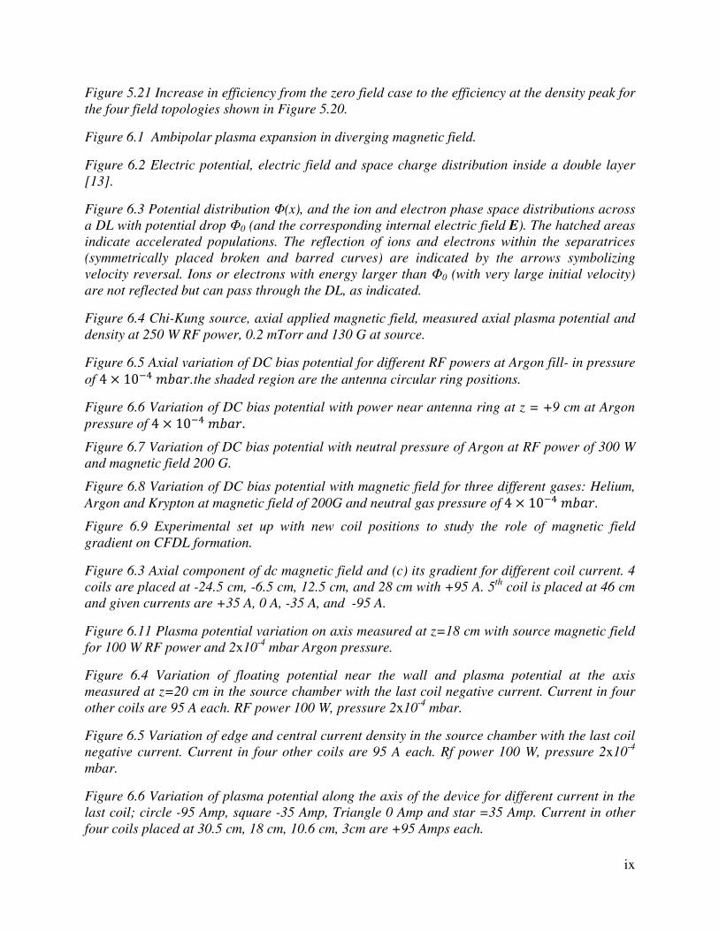
Figure 5.21 Increase in efficiency from the zero field case to the efficiency at the density peak for
the four field topologies shown in Figure 5.20.
Figure 6.1 Ambipolar plasma expansion in diverging magnetic field.
Figure 6.2 Electric potential, electric field and space charge distribution inside a double layer
[13].
Figure 6.3 Potential distribution Φ(x), and the ion and electron phase space distributions across
a DL with potential drop Φ0 (and the corresponding internal electric field E). The hatched areas
indicate accelerated populations. The reflection of ions and electrons within the separatrices
(symmetrically placed broken and barred curves) are indicated by the arrows symbolizing
velocity reversal. Ions or electrons with energy larger than Φ0 (with very large initial velocity)
are not reflected but can pass through the DL, as indicated.
Figure 6.4 Chi-Kung source, axial applied magnetic field, measured axial plasma potential and
density at 250 W RF power, 0.2 mTorr and 130 G at source.
Figure 6.5 Axial variation of DC bias potential for different RF powers at Argon fill- in pressure
of 4 × 10 !"#.the shaded region are the antenna circular ring positions.
Figure 6.6 Variation of DC bias potential with power near antenna ring at z = +9 cm at Argon
pressure of 4 × 10 !"#. Figure 6.7 Variation of DC bias potential with neutral pressure of Argon at RF power of 300 W
and magnetic field 200 G.
Figure 6.8 Variation of DC bias potential with magnetic field for three different gases: Helium,
Argon and Krypton at magnetic field of 200G and neutral gas pressure of 4 × 10 !"#.
Figure 6.9 Experimental set up with new coil positions to study the role of magnetic field
gradient on CFDL formation.
Figure 6.3 Axial component of dc magnetic field and (c) its gradient for different coil current. 4
coils are placed at -24.5 cm, -6.5 cm, 12.5 cm, and 28 cm with +95 A. 5th
coil is placed at 46 cm
and given currents are +35 A, 0 A, -35 A, and -95 A.
Figure 6.11 Plasma potential variation on axis measured at z=18 cm with source magnetic field
for 100 W RF power and 2x10⁻⁴
mbar Argon pressure.
Figure 6.4 Variation of floating potential near the wall and plasma potential at the axis
measured at z=20 cm in the source chamber with the last coil negative current. Current in four
other coils are 95 A each. RF power 100 W, pressure 2x10⁻⁴
mbar.
Figure 6.5 Variation of edge and central current density in the source chamber with the last coil
negative current. Current in four other coils are 95 A each. Rf power 100 W, pressure 2x10⁻⁴
mbar.
Figure 6.6 Variation of plasma potential along the axis of the device for different current in the
last coil; circle -95 Amp, square -35 Amp, Triangle 0 Amp and star =35 Amp. Current in other
four coils placed at 30.5 cm, 18 cm, 10.6 cm, 3cm are +95 Amps each.

x
Figure 6.15 Radial variation of plasma potential with Iv measured at z=18 cm with an L-shaped
emissive probe for 100W RF power and 2x10⁻⁴
mbar Argon pressure.

xi
List of Tables Table 3.1 Parameter regime, length scales and time scales of the present helicon experiment.

1
Chapter 1
Introduction
This chapter initially reviews history of helicon wave research and its applications in brief. Later,
it reviews research on helicon physics relevant to the present thesis work. This will be followed
by the motivation and objectives of the thesis work. Finally, the content and important findings
of this thesis work will be summarized.
1.1 History of Helicon Sources
Plasma is a complex medium which supports many mechanical and electromagnetic
waves. Plasma waves are often classified as electrostatic or electromagnetic waves. Moreover,
the direction of propagation and polarization with respect to the magnetic field is often used for
detailed classification. Magnetic fields introduce anisotropy in the plasma medium for which
magnetized plasmas support a number of waves both in parallel and perpendicular directions.
Right circularly polarized electromagnetic waves propagating along the magnetic field are
typically referred to as whistler [1]. The name is derived from the whistling audio tones with
constant amplitude and declining frequency received in radio receivers during World War I [2]
which were mistaken as flying grenades. Barkhausen [3] explained this phenomenon as the
highly dispersive broadening of a sharp pulse, initiated by lightning that propagates in the
ionosphere. Storey [4] performed measurement on whistling atmospherics and described them as
right handed circularly polarized waves that propagate in free space where ion effects and
collisions were neglected. Helicon waves are whistler waves in a bounded plasma so that the
wavelength is of the order of the plasma dimensions. They are quasi-electromagnetic waves and

2
are different from classical whistler waves which are purely electromagnetic in nature. Helicons
can have both right and left handed polarizations compared to whistlers which have only right
hand polarization.
In 1960, Aigrain [5] suggested the possibilities of observing whistler waves in solid state
plasmas. Aigrain called the wave a helicon wave because the electric field traces out a helix
when the wave propagates along the magnetic field. In an accidental observation, Bowers et al
[6] reported experimental finding of helicon wave while measuring the hall resistivity of a pure
sodium metal using a static magnetic field parallel to the applied oscillating magnetic fields.
They observed a damped oscillation whose frequency was proportional to the applied DC
magnetic field instead of an expected decaying signal in the output of the receiver coil. They
identified the waves as those proposed by Aigrain. Detailed theory for the propagation and
damping of helicon waves was given by Legendy [7] for solid state plasmas and Klosenberg,
McNamara and Thonemann (KMT theory) [8] for gaseous plasmas. Following these theories,
Harding and Thonemann [9] carried experiment in indium and showed good agreement with the
theoretical prediction. Much of the early work on helicon wave was in solid state plasmas
because of an immediate use as a diagnostics for measuring Hall coefficients in pure metals.
Lehane and Thonemann [10] first observed helicon waves in gaseous plasma and found a very
good agreement with wave axial damping rates given by KMT theory. Gallet et al [11] used
helicon waves in gaseous plasma in toroidal ZETA fusion device as a diagnostics for
measurement of plasma density and static magnetic field by measuring the damping of the
helicon waves using magnetic probes.
First use of helicon waves as an efficient source for plasma production was demonstrated
by Boswell [12] who using a double loop antenna at 8 MHz produced plasma of 4x10¹⁸/m3
density with a magnetic field of 1.5 kilo Gauss and RF power of 600 W. This density was higher
by an order from the conventional RF discharges with equal RF input power and magnetic field.
This high efficiency plasma production led to increased interest in helicon plasma physics as
well as its various potential applications. Today they are considered for many applications like
material processing, [13], negative ion production [14], Preionization [15-17] and current drive
[18-19] in fusion plasmas and for space propulsion [20-22].
3
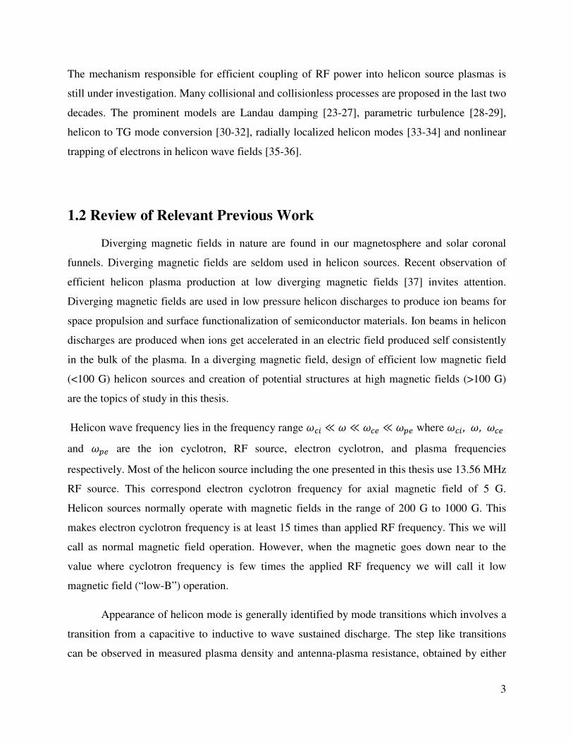
The mechanism responsible for efficient coupling of RF power into helicon source plasmas is
still under investigation. Many collisional and collisionless processes are proposed in the last two
decades. The prominent models are Landau damping [23-27], parametric turbulence [28-29],
helicon to TG mode conversion [30-32], radially localized helicon modes [33-34] and nonlinear
trapping of electrons in helicon wave fields [35-36].
1.2 Review of Relevant Previous Work
Diverging magnetic fields in nature are found in our magnetosphere and solar coronal
funnels. Diverging magnetic fields are seldom used in helicon sources. Recent observation of
efficient helicon plasma production at low diverging magnetic fields [37] invites attention.
Diverging magnetic fields are used in low pressure helicon discharges to produce ion beams for
space propulsion and surface functionalization of semiconductor materials. Ion beams in helicon
discharges are produced when ions get accelerated in an electric field produced self consistently
in the bulk of the plasma. In a diverging magnetic field, design of efficient low magnetic field
(<100 G) helicon sources and creation of potential structures at high magnetic fields (>100 G)
are the topics of study in this thesis.
Helicon wave frequency lies in the frequency range $%& ≪ $ ≪ $%( ≪ $)( where $%&, $, $%( and $)( are the ion cyclotron, RF source, electron cyclotron, and plasma frequencies
respectively. Most of the helicon source including the one presented in this thesis use 13.56 MHz
RF source. This correspond electron cyclotron frequency for axial magnetic field of 5 G.
Helicon sources normally operate with magnetic fields in the range of 200 G to 1000 G. This
makes electron cyclotron frequency is at least 15 times than applied RF frequency. This we will
call as normal magnetic field operation. However, when the magnetic goes down near to the
value where cyclotron frequency is few times the applied RF frequency we will call it low
magnetic field (“low-B”) operation.
Appearance of helicon mode is generally identified by mode transitions which involves a
transition from a capacitive to inductive to wave sustained discharge. The step like transitions
can be observed in measured plasma density and antenna-plasma resistance, obtained by either
4
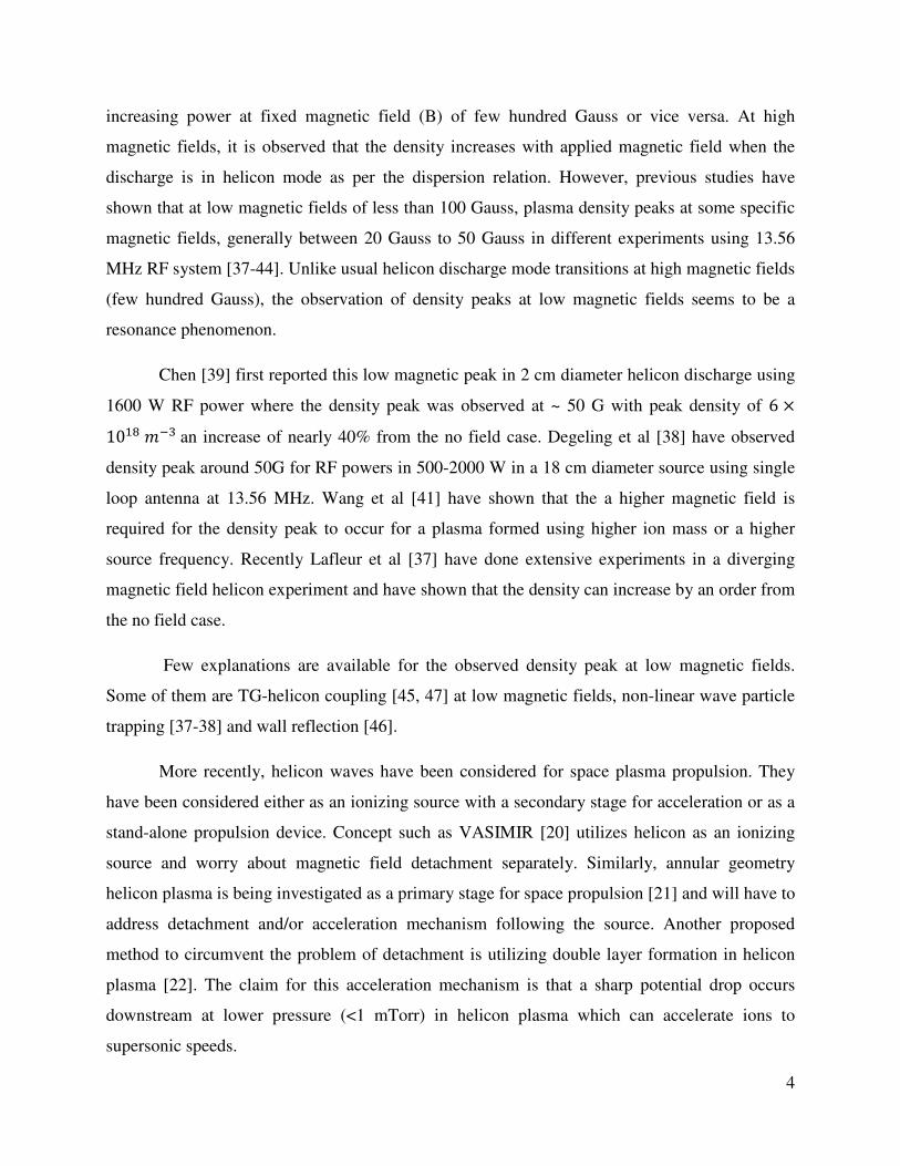
increasing power at fixed magnetic field (B) of few hundred Gauss or vice versa. At high
magnetic fields, it is observed that the density increases with applied magnetic field when the
discharge is in helicon mode as per the dispersion relation. However, previous studies have
shown that at low magnetic fields of less than 100 Gauss, plasma density peaks at some specific
magnetic fields, generally between 20 Gauss to 50 Gauss in different experiments using 13.56
MHz RF system [37-44]. Unlike usual helicon discharge mode transitions at high magnetic fields
(few hundred Gauss), the observation of density peaks at low magnetic fields seems to be a
resonance phenomenon.
Chen [39] first reported this low magnetic peak in 2 cm diameter helicon discharge using
1600 W RF power where the density peak was observed at ~ 50 G with peak density of 6 ×10,- . an increase of nearly 40% from the no field case. Degeling et al [38] have observed
density peak around 50G for RF powers in 500-2000 W in a 18 cm diameter source using single
loop antenna at 13.56 MHz. Wang et al [41] have shown that the a higher magnetic field is
required for the density peak to occur for a plasma formed using higher ion mass or a higher
source frequency. Recently Lafleur et al [37] have done extensive experiments in a diverging
magnetic field helicon experiment and have shown that the density can increase by an order from
the no field case.
Few explanations are available for the observed density peak at low magnetic fields.
Some of them are TG-helicon coupling [45, 47] at low magnetic fields, non-linear wave particle
trapping [37-38] and wall reflection [46].
More recently, helicon waves have been considered for space plasma propulsion. They
have been considered either as an ionizing source with a secondary stage for acceleration or as a
stand-alone propulsion device. Concept such as VASIMIR [20] utilizes helicon as an ionizing
source and worry about magnetic field detachment separately. Similarly, annular geometry
helicon plasma is being investigated as a primary stage for space propulsion [21] and will have to
address detachment and/or acceleration mechanism following the source. Another proposed
method to circumvent the problem of detachment is utilizing double layer formation in helicon
plasma [22]. The claim for this acceleration mechanism is that a sharp potential drop occurs
downstream at lower pressure (<1 mTorr) in helicon plasma which can accelerate ions to
supersonic speeds.
5
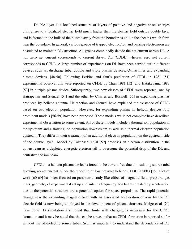
Double layer is a localized structure of layers of positive and negative space charges
giving rise to a localized electric field much higher than the electric field outside double layer
and is formed in the bulk of the plasma away from the boundaries unlike the sheaths which form
near the boundary. In general, various groups of trapped electron/ion and passing electron/ion are
postulated to maintain DL structure. All groups combinedly decide the net current across DL. A
non zero net current corresponds to current driven DL (CDDL) whereas zero net current
corresponds to CFDL. A large number of experiments on DL have been carried out in different
devices such as, discharge tube, double and triple plasma devices, Q-machines and expanding
plasma devices. [48-50]. Following Perkins and Sun’s prediction of CFDL in 1981 [51]
experimental observations were reported on CFDL by Chan 1981 [52] and Hatakeyama 1983
[53] in a triple plasma device. Subsequently, two new classes of CFDL were reported; one by
Hairapetian and Stenzel [54] and the other by Charles and Boswell [55] in expanding plasmas
produced by helicon antenna. Hairapetian and Stenzel have explained the existence of CFDL
based on two electron population. However, for expanding plasma in helicon devices four
prominent models [56-59] have been proposed. These models while not complete have described
experimental observation to some extent. All of these models include a thermal ion population in
the upstream and a flowing ion population downstream as well as a thermal electron population
upstream. They differ in their treatment of an additional electron population on the upstream side
of the double layer. Model by Takahashi et al [59] proposes an electron distribution in the
downstream as a depleted energetic electron tail to overcome the potential drop of the DL and
neutralize the ion beam.
CFDL in a helicon plasma device is forced to be current free due to insulating source tube
allowing no net current. Since the reporting of low pressure helicon CFDL in 2003 [55] a lot of
work [60-69] has been focused on parametric study like effect of magnetic field, pressure, gas
mass, geometry of experimental set up and antenna frequency. Ion beams created by acceleration
due to the potential structure are a potential option for space propulsion. The rapid potential
change near the expanding magnetic field with an associated acceleration of ions by the DL
electric field is now being employed in the development of plasma thrusters. Meige et al [70]
have done 1D simulation and found that finite wall charging is necessary for the CFDL
formation and it may be noted that this can be a reason that no CFDL formation is reported so far
without use of dielectric source tubes. So, it is important to understand the dependence of DL

6
strength on various plasma parameters as well as magnetic field geometry along with the role of
wall charging on CFDL formation.
Charles and Boswell [71] studied the role of magnetic field on CFDL formation. By
increasing the magnetic field they have observed ion beam formation in downstream plasma for
a critical magnetic field of 50 G in the source. The source potential and density increased
simultaneously at 50 G but in the downstream plasma the effect was little. Ion magnetization at
50 G is attributed to this transition from an expanding plasma to a plasma containing a CFDL.
When the ion is magnetized the ion loss to the radial wall decreases and amounted to the density
rise. Similar results were obtained by Takahashi et al [69] in EMPI source have shown that for
two different dielectric source tubes of radii of 3.25 cm and 2.3 cm, the CFDL is formed for
125 G and 195 G respectively the values of these magnetic fields also are the magnetic fields
where the ions got magnetized.
Though the observations of the CFDL were reported by many authors, the location and
strength of the CFDL dependency on magnetic field gradient and magnetic field topology is not
clear. The role of magnetic field gradient and its location was studied by Sutherland et al [67],
Byhring et al [63] and Schroder et al [64]. Sutherland et al. [67] showed that the CFDL strength
could be scaled by a factor of at least 2 in a bigger system and that the double layer presumably
forms in the vicinity of maximal gradient of the magnetic field. Byhring et al [63] changed the
magnetic field gradient by using an extra coil in which the current is passed in the same direction
as the other coils. So by increasing the current in their last coil they could decrease the magnetic
field gradient which location was much inside the source plasma. They have found that CFDL
vanished for higher last coil currents which were confirmed by RFEA measurements. A study on
independent effects of geometric expansion, magnetic field and field gradient along with its
location are studied by Schroder et al [64] in VINETA device. For magnetic field gradient
location coinciding with the geometric expansion they have found the CFDL strength is highest.
1.3 Motivation and objective
The primary objective of the work described here in the thesis is to develop a helicon
plasma source in geometrically and magnetically diverging configuration. Design, fabricate and
operation of each subsystems have been carried out during the thesis work. This thesis aims to

7
study characterizing discharge modes, investigating the mechanism responsible for low magnetic
field density peak, studying double layer and its relation with the wall charging.
1.4 Description of chapters and main findings
The work described in this thesis has two main elements; (1) Development of
experimental system and (2) Physics studies in the system. This thesis consists of seven chapters.
The first chapter is an introduction to helicon research and also includes the motivation and
objective of the thesis. The second chapter describes theory of helicon wave dispersion, wave
mode structure, physics of discharge mode transitions and power coupling to plasma. In the third
chapter experimental set up and its sub-systems along with various diagnostics used are
discussed. After describing the previous studies, experimental set up and diagnostics in chapter
1, 2 and 3, the initial characterization of the RF plasma produced in the linear plasma device is
described in Chapter four. Once the system is evacuated to 1×10⁻⁶ mbar, Argon gas is fed into
the system at 5×10⁻³ mbar pressure through the end flange connected to the source chamber.
After that RF power is slowly delivered to the antenna through the matching network. Gas
breakdown is observed at few W (< 10 W) of RF power with almost no reflected power without
magnetic field. We have obtained various plasma discharges in the pressure range of 1×10⁻⁴
mbar to 1×10⁻² mbar by applying suitable magnetic field in the span of 0 to 280 Gauss and RF
power in the range of few Watts to 1.5 kW. Thus the neutral pressure, magnetic field and RF
power are the controlling parameters of our experiment. Mode transitions are studied by
measuring density and load capacitance values (a measure of antenna-plasma coupling) for
different pressures by varying the RF power. By increasing the pressure, Helicon operation
regime is achieved for 112 Gauss magnetic field. The values of RF power at which the
transitions occurred are lower for higher neutral pressures. Helicon m=+1 modes are
characterized by measuring the radial and axial wave profile. The axial wavelength of the
helicon waves are measured by measuring the axial phase variation using a single loop B-dot
probe with respect to another reference B-dot probe phase fixed at a constant radial and axial
location. Axial plasma potential is measured with a floating emissive probe at low pressure, 600
W RF power and 288 Gauss magnetic field. Plasma potential drops of ~8Te are observed
over~1000 λD distance. These above mentioned preliminary results along with the details of the
experimental set up and its capabilities are published in Rev. Sci. Instrum. 83, 063501 (2012).

8
Low field helicon experiments in a diverging magnetic field configuration are discussed
in chapter five. Experiments are carried out using argon gas with m = +1 right helical antenna
operating at 13.56 MHz by varying the magnetic field from 0 Gauss to 100 Gauss (G). The
plasma density 18 cm away from antenna centre varies with varying the magnetic field at
constant input power and gas pressure and reaches to its peak value at a magnetic field value of ~
25 G. Another peak of smaller magnitude in density has been observed near 50 G. Measurement
of amplitude and phase of the axial component of the wave using magnetic probes for two
magnetic field values corresponding to the observed density peaks indicated the existence of
radial modes. Measured parallel wave number together with the estimated perpendicular wave
number suggests oblique mode propagation of helicon waves along the resonance cone boundary
for these magnetic field values. Further, the observations of larger floating potential fluctuations
measured with Langmuir probes at those magnetic fields values, indicate that near resonance
cone boundary, these electrostatic fluctuations are proposed to take energy from helicon wave
and dump power to the plasma causing density peaks. The results are published in Physics of
Plasmas 20, 042119 (2013). Asymmetry in density peaks on either side of an m = +1 half helical
antenna is observed both in terms of peak position and its magnitude with respect to magnetic
field variation. However, the density peaks occurred at different critical magnetic fields on both
sides of antenna. Depending upon the direction of the magnetic field, in the m = +1 propagation
side, the main density peak has been observed around 27 Gauss (G) of magnetic field. On this
side the density peaks around 5 G, corresponding to electron cyclotron resonance (ECR) is not
very pronounced whereas on the m = -1 propagation side, very pronounced ECR peak has been
observed around 5 G. Another prominent density peak around 13 G has also been observed on m
= -1 side. However, no peak has been observed around 27 G on the m = -1 side. The density peak
data is also supported by the light intensity measurements on both sides of the antenna.
Reversing the magnetic field direction symmetrically reverses all the density peak observations.
Observation of ECR peak around 5 G on m = -1 side is explained on the basis of the polarization
reversal effect of circularly polarized waves in a bounded plasma while the other peaks on either
side are explained with the help of cyclotron resonance for obliquely propagating helicon waves.
The measured antenna-plasma resistance, a measure of power coupled to the plasma by the
antenna, can only be explained if density variations on both sides of the antenna are taken into
account. The results are published in Physics of Plasmas 20, 012123 (2013). Experiments were

9
further performed by changing the divergence of the magnetic field near the helicon antenna. By
increasing the divergence it is observed that the antenna plasma coupling increases. A helicon
antenna generally has a k-spectrum but when the antenna is in a uniform magnetic field, the
resonance cone propagation is achieved only for a single mode at a certain magnetic field. With a
diverging magnetic field, many modes can have resonance cone propagation at a single magnetic
field value at the antenna centre. The efficient coupling is explained on the basis of multiple
mode absorption near antenna through resonance cone absorption for different magnetic fields
available near the antenna. This conjecture is further strengthened by the observed higher values
of density maintained for more values of magnetic field of 20 – 60 Gauss i.e. widening of the
density peak as the divergence is increased. The manuscript based on these results is ready for
submission. The resonance cone absorption is further studied at the downstream of the plasma
where the magnetic field reduces to ~10 Gauss from ~100 Gauss at the source. Phase
measurements show that helicon waves are stationary near the antenna and propagate only in the
diffusion chamber. Density peaks are observed in the downstream where the resonance cone
propagation angles are near the wave propagation angles. These results are reproduced for
different power and pressure values. Normal ECR absorption at location where magnetic field ~
5 Gauss, is observed in the downstream by varying the magnetic field configuration using an
extra coil and supplying negative current to it w. r .t to other coils. The manuscript based on
these results is ready to be submitted for publication.
Chapter six discusses the study of current free double layer near the geometrical
expansion region of the plasma and the relation of this potential structure to charging of the
dielectric wall and magnetic field gradient. Experiments are carried out to study the role of
magnetic field gradient near the geometrical expansion location. The experiments are done at
100 W RF power and 2×10⁻⁴ mbar with different magnetic field gradients near the geometrical
expansion of the chamber. It is observed that the increasing the magnetic field gradient, the
CFDL structure evolved from a single weak CFDL to a multiple structure which consists of a
strong CFDL and a weak CFDL. The plasma potential in the source dielectric chamber is with
respect to the floating glass wall. The wall charges to a higher negative potential and lifts the
plasma potential in the source chamber to higher positive values at low pressures. So the
parametric dependence of dielectric wall charging caused by RF potential fluctuation induced
into the plasma through the capacitance of the glass tube is studied near the antenna for different

10
RF power, neutral pressure, magnetic field and gas mass. Conclusions and future scopes are
presented in the last chapter.

11
References
[1] Paul Murray Bellan. Fundamentals of plasma physics. Cambridge University Press, 2006.
[2] R. W. Boswell, A Study of Wave in Gaseous Plasma, Ph. D. Thesis, Flinders University, Adelaida, Australia (1974)
[3] Barkhausen, Heinrich. "Whistling tones from the Earth." Proceedings of the Institute of
Radio Engineers 18, no. 7 (1930): 1155-1159.
[4] Storey, L. R. O. "An investigation of whistling atmospherics." Philosophical Transactions of
the Royal Society of London. Series A, Mathematical and Physical Sciences 246, no. 908 (1953): 113-141.
[5] Aigrain P, Proc. Int. Conf. on Semiconductor Physics, Prague (London: Butterworths) p 224(1960)
[6] Bowers, R., C. Legendy, and F. Rose. "Oscillatory galvanomagnetic effect in metallic sodium." Physical Review Letters 7, no. 9 (1961): 339-341.
[7] Legendy, C. R. (1964). Macroscopic theory of helicons. Physical Review, 135(6A), A1713.
[8] Harding, G. N., and P. C. Thonemann. "A study of helicon waves in indium." Proceedings of
the Physical Society 85, no. 2 (1965): 317.
[9] Klozenberg, J. P., B. McNamara, and P. C. Thonemann. "The dispersion and attenuation of helicon waves in a uniform cylindrical plasma." J. Fluid Mech 21, no. 3 (1965): 545-563.
[10] Lehane, J. A., and P. C. Thonemann. "An experimental study of helicon wave propagation in a gaseous plasma." Proceedings of the Physical Society 85, no. 2 (1965): 301.
[11] Gallet, R. M., Richardson, J. M., Wieder, B., Ward, G. D., & Harding, G. N. (1960). Microwave whistler mode propagation in a dense laboratory plasma. Physical Review Letters, 4(7), 347.
[12] Boswell, R. W. "Plasma production using a standing helicon wave." Physics Letters A 33, no. 7 (1970): 457-458.
[13] Perry, A. J., D. Vender, and R. W. Boswell. "The application of the helicon source to plasma processing." Journal of Vacuum Science & Technology B: Microelectronics and
Nanometer Structures 9, no. 2 (1991): 310-317.
[14] Wang, S. J., et al. "Observation of enhanced negative hydrogen ion production in weakly magnetized RF plasma." Physics Letters A 313.4 (2003): 278-283.
[15] Stubbers, Robert A., et al. "Compact toroid formation using an annular helicon preionization source." AIAA-2007-5307, 43rd Joint Propulsion Conference, Cincinnati, OH, 2007.

12
[16] Masters, B. C., et al. "Magnetic and Thermal Characterization of An ELM Simulating Plasma (ESP) With Helicon Pre-Ionization." Fusion Engineering 2005, Twenty-First IEEE/NPS
Symposium on. IEEE, 2005.
[17] Jeon, S. J., W. Choe, G. C. Kwon, J. H. Kim, H. S. Yi, S. W. Herr, H. Y. Chang, and D. I. Choi. "Coupling characteristics of a helicon antenna in KAIST-Tokamak plasma." In SOFT:
Symposium on fusion technology. 1998.
[18] Loewenhardt, P. K., B. D. Blackwell, R. W. Boswell, G. D. Conway, and S. M. Hamberger. "Plasma production in a toroidal heliac by helicon waves." Physical review letters 67, no. 20 (1991): 2792.
[19] Tripathi, S. K. P., and D. Bora. "Current drive by toroidally bounded whistlers." Nuclear
fusion 42, no. 10 (2002): L15.
[20] Diaz, FR Chang. "An overview of the VASIMR engine: High power space propulsion with RF plasma generation and heating." In AIP Conference Proceedings, vol. 595, p. 3. 2001.
[21] Brian Beal, Alec Gallimore, David Morris, Christopher Davis, and Kristina Lemmer “Development of an annular helicon source for electric propulsion applications.” Defense Technical Information Center, 2006.
[22] West, Michael D., Christine Charles, and Rod W. Boswell. "Testing a helicon double layer thruster immersed in a space-simulation chamber." Journal of Propulsion and Power 24, no. 1 (2008): 134-141.
[23] F. F. Chen, “Plasma Ionization by Helicon Waves,” Plasma Physics and Controlled
Fusion, vol. 33, no. 4, pp. 26, 1991.
[24] Ellingboe, A. R., R. W. Boswell, J. P. Booth, and N. Sadeghi. "Electron beam pulses produced by helicon‐wave excitation." Physics of Plasmas 2 (1995): 1807.
[25] Molvik, A. W., A. R. Ellingboe, and T. D. Rognlien. "Hot-electron production and wave structure in a helicon plasma source." Physical Review Letters 79.2 (1997): 233.
[26] Blackwell, David D., and Francis F. Chen. "Time-resolved measurements of the electron energy distribution function in a helicon plasma." Plasma Sources Science and Technology 10.2 (2001): 226.
[27] F. F. Chen, and D. D. Blackwell, “Upper Limit to Landau Damping in Helicon Discharges,” Physical Review Letters, vol. 82, no. 13, pp. 2677, 1999.
[28] Krämer, M., Aliev, Y. M., Altukhov, A. B., Gurchenko, A. D., Gusakov, E. Z., and Niemi, K. (2007). Anomalous helicon wave absorption and parametric excitation of electrostatic fluctuations in a helicon-produced plasma. Plasma Physics and Controlled Fusion, 49(5A), A167.
[29] Akhiezer, A. I., Mikhailenko, V. S., and Stepanov, K. N. (1998). Ion-sound parametric turbulence and anomalous electron heating with application to helicon plasma sources. Physics
Letters A, 245(1), 117-122.

13
[30] Borg, G. G., and R. W. Boswell. "Power coupling to helicon and Trivelpiece–Gould modes in helicon sources." Physics of Plasmas 5 (1998): 564.
[31] Arnush, Donald. "The role of Trivelpiece–Gould waves in antenna coupling to helicon waves." Physics of Plasmas 7 (2000): 3042.
[32] Shamrai, Konstantin P., and Vladimir B. Taranov. "Volume and surface rf power absorption in a helicon plasma source." Plasma Sources Science and Technology 5.3 (1996): 474.
[33] B. N. Breizman, and A. V. Arefiev, “Radially Localized Helicon Modes in Nonuniform Plasma,” Physical Review Letters, vol. 84, no. 17, pp. 4, 2000.
[34] Chen, Guangye, Alexey V. Arefiev, Roger D. Bengtson, Boris N. Breizman, Charles A. Lee, and Laxminarayan L. Raja. "Resonant power absorption in helicon plasma sources." Physics of plasmas 13 (2006): 123507.
[35] Degeling, A. W., C. O. Jung, R. W. Boswell, and A. R. Ellingboe. "Plasma production from helicon waves." Physics of Plasmas 3 (1996): 2788.
[36] Degeling, A. W., and R. W. Boswell. "Modeling ionization by helicon waves." Physics of
Plasmas 4 (1997): 2748.
[37] Lafleur, T., C. Charles, and R. W. Boswell. "Characterization of a helicon plasma source in low diverging magnetic fields." Journal of Physics D: Applied Physics 44, no. 5 (2011): 055202.
[38] Degeling, A. W., C. O. Jung, R. W. Boswell, and A. R. Ellingboe. "Plasma production from helicon waves." Physics of Plasmas 3 (1996): 2788.
[39] Chen, F. F., X. Jiang, J. D. Evans, G. Tynan, and D. Arnush. "Low-field helicon discharges." Plasma Physics and Controlled Fusion 39, no. 5A (1997): A411.
[40] Lho, Taihyeop, Noah Hershkowitz, J. Miller, W. Steer, and Gon-Ho Kim. "Azimuthally symmetric pseudo-surface and helicon wave propagation in an inductively coupled plasma at low magnetic field." Physics of Plasmas 5 (1998): 3135.
[41] Wang, S. J., J. G. Kwak, C. B. Kim, and S. K. Kim. "Observation of enhanced negative hydrogen ion production in weakly magnetized RF plasma." Physics Letters A 313, no. 4 (2003): 278-283.
[42] Sato, G., W. Oohara, and R. Hatakeyama. "Efficient plasma source providing pronounced density peaks in the range of very low magnetic fields." Applied physics letters 85, no. 18 (2004): 4007-4009.
[43] Wang, S. J., Jong-Gu Kwak, S. K. Kim, and Suwon Cho. "Experimental study on the density peaking of an RF plasma at a low magnetic field." Journal of Korean Physical Society 51 (2007): 989.
[44] Sato, G., W. Oohara, and R. Hatakeyama. "Experimental characterization of a density peak at low magnetic fields in a helicon plasma source." Plasma Sources Science and Technology 16, no. 4 (2007): 734.

14
[45] S. Cho, “The resistance peak of helicon plasmas at low magnetic fields”, Physics of Plasmas 13, 033504 (2006).
[46] Chen, Francis F. "The low-field density peak in helicon discharges." Physics of Plasmas 10 (2003): 2586.
[47] Shamrai, Konstantin P., and Vladimir B. Taranov. "Volume and surface rf power absorption in a helicon plasma source." Plasma Sources Science and Technology 5, no. 3 (1996): 474.
[48] Charles, C. "A review of recent laboratory double layer experiments." Plasma Sources
Science and Technology 16, no. 4 (2007): R1.
[49] Singh, N. (2011). Current-free double layers: A review. Physics of Plasmas, 18(12), 122105-122105.
[50] Hershkowitz, Noah. "Review of recent laboratory double layer experiments." Space science
reviews 41, no. 3-4 (1985): 351-391.
[51] Perkins, Francis W., and Y. C. Sun. "Double layers without current." Physical Review
Letters 46 (1981): 115-118.
[52] Chan, Chung, Noah Hershkowitz, and G. L. Payne. "Laboratory double layers with no external fields." Physics Letters A 83, no. 7 (1981): 328-330.
[53] Hatakeyama, R., Y. Suzuki, and N. Sato. "Formation of electrostatic potential barrier between different plasmas." Physical Review Letters 50, no. 16 (1983): 1203.
[54] Hairapetian, G., and R. L. Stenzel. "Observation of a stationary, current-free double layer in a plasma." Physical review letters 65, no. 2 (1990): 175.
[55] Charles, C., & Boswell, R. (2003). Current-free double-layer formation in a high-density helicon discharge. Applied Physics Letters, 82(9), 1356-1358.
[56] Lieberman, M. A., C. Charles, and R. W. Boswell. "A theory for formation of a low pressure, current-free double layer." Journal of Physics D: Applied Physics 39, no. 15 (2006): 3294.
[57] Chen, Francis F. "Physical mechanism of current-free double layers." Physics of plasmas 13 (2006): 034502.
[58] Ahedo, Eduardo, and Manuel Martínez Sánchez. "Theory of a Stationary Current-Free Double Layer in a Collisionless Plasma." Physical review letters 103, no. 13 (2009): 135002.
[59] Takahashi, Kazunori, Christine Charles, Rod W. Boswell, and Tamiya Fujiwara. "Electron Energy Distribution of a Current-Free Double Layer: Druyvesteyn Theory and Experiments." Physical Review Letters 107, no. 3 (2011): 035002.
[60] Charles, Christine, and R. W. Boswell. "Laboratory evidence of a supersonic ion beam generated by a current-free “helicon” double-layer." Physics of Plasmas 11 (2004): 1706.

15
[61] Sun, Xuan, Amy M. Keesee, Costel Biloiu, Earl E. Scime, Albert Meige, Christine Charles, and Rod W. Boswell. "Observations of ion-beam formation in a current-free double layer." Physical review letters 95, no. 2 (2005): 025004.
[62] Cohen, Samuel Alan, N. S. Siefert, S. Stange, R. F. Boivin, E. E. Scime, and F. M. Levinton. "Ion acceleration in plasmas emerging from a helicon-heated magnetic-mirror device." Physics of Plasmas 10 (2003): 2593.
[63] Byhring, H. S., C. Charles, Å. Fredriksen, and R. W. Boswell. "Double layer in an expanding plasma: Simultaneous upstream and downstream measurements." Physics of plasmas 15 (2008): 102113.
[64] Schröder, T., O. Grulke, and T. Klinger. "The influence of magnetic-field gradients and boundaries on double-layer formation in capacitively coupled plasmas." EPL (Europhysics
Letters) 97, no. 6 (2012): 65002.
[65] Wiebold, Matt, Yung-Ta Sung, and John E. Scharer. "Experimental observation of ion beams in the Madison Helicon eXperiment." Physics of Plasmas 18 (2011): 063501.
[66] Saha, S. K., S. Raychaudhuri, S. Chowdhury, M. S. Janaki, and A. K. Hui. "Two-dimensional double layer in plasma in a diverging magnetic field." Physics of Plasmas 19 (2012): 092502.
[67] Sutherland, O., Charles, C., Plihon, N., and Boswell, R. W. (2005). Experimental evidence of a double layer in a large volume helicon reactor. Physical review letters, 95(20), 205002.
[68] Thakur, Saikat Chakraborty, Alex Hansen, and Earl E. Scime. "Threshold for formation of a stable double layer in an expanding helicon plasma." Plasma Sources Science and Technology
19, no. 2 (2010): 025008.
[69] Takahashi, K., Charles, C., Boswell, R. W., and Fujiwara, T. (2010). Double-layer ion acceleration triggered by ion magnetization in expanding radiofrequency plasma sources. Applied Physics Letters, 97(14), 141503-141503.
[70] Albert Meige, Numerical modeling of low-pressure plasmas: applications to electric double layers, Thesis, Australian National University (2006).
[71] Charles, C., and R. W. Boswell. "The magnetic-field-induced transition from an expanding plasma to a double layer containing expanding plasma." Applied Physics Letters 91, no. 20 (2007): 201505-201505.

16
Chapter 2
Helicon Physics
2.1 Introduction
The low frequency right circularly polarized electromagnetic waves in plasma propagating
parallel to the magnetic field are known as the whistler waves [1]. Helicon waves are whistler
waves in bounded plasmas where the wavelength is of the order of the plasma dimensions.
Whistler waves lose their pure electromagnetic character and become quasi-electromagnetic
helicon waves when bounded. Helicons can have both the right and left handed polarizations
compared to the unbounded medium whistlers which have only right handed polarization.
Klozenberg, McNamra and Thonemann [2] first derived the detailed dispersion relation of
helicon waves with their mode structure in a gaseous plasma with a vacuum boundary. Blevin
and Christiansen [3] obtained the dispersion in a non-uniform plasma. Ferrari and Klozenberg [4]
derived the dispersion and attenuation of helicon waves in a plasma with perfectly conducting
boundaries.
A brief derivation of the helicon dispersion from cold plasma dielectric tensor is presented.
Quasiparallel oblique propagation of right polarized electromagnetic waves is discussed with
importance to resonance cone propagation. The mode structure of helicon waves in cylindrical
uniform plasmas and the effect of density gradients on these structures are discussed. Another
important feature of helicon antenna produced plasma is the mode transitions. RF discharges can
be sustained by an electric field of capacitive, inductive or wave origin. An RF inductive plasma
is known to support both capacitive and inductive mode. Helicon plasma is a unique discharge in
which the discharge can be sustained by all the three modes namely capacitive, inductive and
wave or helicon.

17
2.2 Derivation of dispersion relation
Ordinary fluids such as air or water can support only a few types of oscillations or waves. For
example, sound waves in air are due to the propagation of pressure disturbances. Water surface
waves are due to the cohesion (surface tension) and inertia of water. The dispersion relation
relates the wavelength to the frequency of the wave. This relation can describe the wave motion
by providing information about the wavelength and phase velocity for a given frequency. For
example, even a vacuum can support a type of wave: electromagnetic radiation.
2.2.1 Vacuum Waves
The dispersion relation for electromagnetic radiation can be found from Maxwell's equations in
vacuum (using SI units):
0 ∙ 2 = (2. 1 )
0 ∙ 3 = (2. 2 )
0 × 2 = − 4345 (2. 3 )
0 × 3 = 6 4245 (2. 4 )
By combining Equation 2.3 and Equation 2.4, one obtains the differential equation for the
electric field:
0778 × 0778 × 2778 = − 6 4277845 (2. 5 )
Carrying out Fourier analysis while looking for harmonic solutions of
type 9, : = 9;, :;<&(>? @A), Equation 2.5 can transform spatial derivatives into wave vectors
and time derivatives into frequencies as
C778 × C778 × 2778 = − 6 2778 (2. 6 )

18
revealing a relationship between electric field, wave vector, and frequency. Then, using a vector
identity and Eq. 2.6 one obtains an equation for the wave electric field:
D6 − CE 2778 = (2. 7 )
For the non-trivial solution with :7778 ≠ 0, it is necessary that:
6 = C, G C = ±6 (2. 8 )
which is the dispersion relation for electromagnetic waves in vacuum. This dispersion relation
indicates that the phase velocity I)J = $ K⁄ is of constant magnitude c. The group velocity (the
velocity of energy flow, for a wave packet composed of many different wavenumbers IMN = is
the same for any wave number, so there is no dispersion in the sense that waves of different
wavelengths in a wave packet all propagate with the same phase and group velocities. The
situation can be very different in plasma, as will be seen later.
Plasma can be considered as a dielectric medium with long range electromagnetic forces leading
to collective behavior for which a perturbation at one place in plasma can affect the plasma at
other place. The motion of charged particles in the presence of electric and magnetic fields
created by the externally applied or self consistently generated sources of charge density and
current density makes the dynamics complicated. The dispersion relation relates the wave
frequency to the wave number in a medium and the wave phase velocity is defined as I = $/K.
The wave number of an electromagnetic weave in vacuum is related to the frequency by the
velocity = PQ, so that wavelength can be obtained if frequency is given. But in a complex
medium like magnetized plasma with collective behaviour, the medium becomes anisotropic and
a detailed derivation of the dispersion relation is tedious. What follows now is the derivation of
the cold plasma dielectric tensor.
19
Cold plasma is one in which the thermal velocities of the particles are much smaller than the
phase velocities of the waves (IAJ ≪ $ K⁄ ). Magnetized plasma being an anisotropic medium for
electromagnetic waves supports various kinds of waves. Since plasma consists of light electrons
and heavy ions, characteristic frequencies range from low frequency ion cyclotron frequency to
high frequency electron cyclotron frequency. A general fluid description method considering
both ions and electrons will be presented for finding normal modes in collisionless, magnetized
plasmas. Cold plasma wave equations are derived by the ion and electron equations of motion in
the electromagnetic fields and the Maxwell’s equation [5]. The momentum equation gives the
evolution of current produced in the plasma because of applied (or self generated)
electromagnetic fields which in turn evolve following the Maxwell’s equations. The solutions of
these self consistent equations give out the normal modes.
The seed of theory of helicon wave lies in the theory of whistler wave. Since helicon wave is a
bounded whistler the theory becomes more involved and complex. It becomes even more
complex when plasma and/or magnetic field are non-uniform. Moreover, at the boundary the
very existence of surface wave (Trivelpiece-Gould mode) invites the possibility of coupling
between helicon and TG. The basic theory of whistler waves is covered in textbooks such as Stix
[5], Swanson [6] and Bellan [1]. In order to interpret and classify the wave experiments
considered in the present thesis, plasma waves are introduced theoretically in this chapter. The
derivation follows the well established approach of Stix [5], Swanson [6] and Bellan [1] and the
waves are classified by their different roots in the cold plasma wave dispersion relation. Starting
from Maxwell’s’ equations and the cold plasma particle equations, the cold magnetized plasma
dielectric tensor and the dispersion relation are derived in section 2.1.2 for both parallel and
perpendicular propagation. For the frequency ranges of interest of this thesis, taking electron
mass into consideration, two solutions as a slow and a fast wave are obtained. In section 2.3,
resonance cone propagation of an R-wave is discussed when the finite angle of propagation w.r.t
magnetic field, coincides with the resonance cone angle. Wave field components are derived in
section 2.4 for laboratory experiments where the plasma is bounded in a cylindrical boundary. A
brief discussion on the effect of non-uniform radial density profiles on helicon wave propagation
is presented in section 2.4. Different mechanisms of helicon power deposition in plasma leading
to dense plasmas are described in Section 2.6. Finally the summary of the chapter is presented.

20
2.2.2 Plasma Waves
The reason plasma waves are so different from vacuum waves is that, in the presence of a
plasma, the source terms in Maxwell's equations are non-zero. Charge and current density play a
significant role in altering the simple character of vacuum electromagnetic waves. Maxwell's
equations become:
0 ∙ 2 = RS (2. 9 )
0 ∙ 3 = (2. 10 )
0 × 2 = − 4345 (2. 11 )
0 × 3 = TU + 6 4245 (2. 12 )
In the above equations, V and W (absent in vacuum) are respectively the charge and current
density and X;,Y; are permeability and permittivity of free space with as the speed of light.
Taking the curl of Eq. 2.11 and substituting into Eq. 2.12 results in a wave equation:
0778 × 0778 × 2778 = − 6 4277845 − T 4U845 (2. 13 )
The plasma current W8 due to a plasma wave is related to the particle velocities. Modelling the
plasma as a mix of fluids of several kinds of particles (electrons and different ion species),
U8 = ∑ [\\]778\ ≡ _8 ∙ 2778\ (2. 14 )
where the index s in the sum denotes the plasma species (electron & ion), and the conductivity
tensor a78 is defined by Eq. 2.14. By substituting the Lorentz force into Newton's second law
21
(neglecting pressure term as this is a cold plasma model), one obtains the equation of motion for
the fluid of different species,
\ b]778\b5 = [\c2778 + ]778\ × 3778d (2. 15 )
Where e and fe are the charge and mass of the particle and Ie(#, g) is its velocity. Solving for
I8e in terms of the components of :7778, and plugging into Eq. 2.14 allows one to determine the
conductivity tensor elements.
To proceed to obtain a dispersion relation, again Fourier analyze Eq. 2.11 in time and space with
a look out for harmonic solutions like I, 9, : = 9;, :;<&(>? @A):
C778 × C778 × 2778 = − 6 2778 − hT_8 ∙ 2778 (2. 16 )
Suppose we consider “cold” plasma, meaning one in which plasma beta << 1. This corresponds
to the limit in which kinetic pressure is negligible. Each species of particle will also have an
equation of motion of the form Eq. 2.15. Linearizing this equation assuming zeroth order
quantity to be constant we can obtain equations with three components, the sign of charges, ±1, is given by Ye,
−h]i,\ = S\[\ 2i + S\[\ ]j3 = S\[\ 2i + ]j6 (2. 17 )
−h]j,\ = S\[\ 2j − S\[\ ]j3 = S\[\ 2i − ]j6 (2. 18 )
−h]k,\ = S\[\ 2k (2. 19 )

22
Our goal is to obtain an expression for the current W8 in terms of the electric field, from which we
can get the components of a78. This relationship can be obtained by finding the velocities of the
individual particle species in terms of the electric field from the equations of motion.
Solving the z-component of the equation of motion above for Il
]k,\ = h S\[\ 2k (2. 20 )
The current in the z-direction is thus,
Uk,\ = S\[]k (2. 21 )
We can now determine zz component of am,
nk,\ = _kk2k = S\[ Dh S\[\ 2kE = Dh [\E (2. 22 )
Therefore, _kk = h [\ (2. 23 )
We can also consider the equation for the o pand qr directions. Multiplying the os component of the
equation of motion by ω,
]i,\ = hS\ [\ 2i + h6,\]j,\ (2. 24 )
Substituting the qs components of the equation of motion,
−h]j,\ = S\[\ 2j − ]i,\6,\ (2. 25 )
tu vuw, ]i,\ = hS\ [\ 2i + 6,\ x− S\[\ 2j + ]i,\6,\y

23
= hS\ [\ 2i − S\6,\ [\ 2j + ]i,\ 6,\ (2. 26 )
Isolating I? and dividing by the coefficient,
]i,\ = hS\ [\ 6,\ 2i − S\[\
6,\ 6,\ 2j (2. 27 )
With the velocity we can form the current density
ni,\ = \[]i,\ = h [\ 6,\ 2i − [\
6,\ 6,\ 2j (2. 28 )
The current can also be written using conductivity tensor components,
ni,\ = _ii,\2i + _ij,\2j + _ik,\2k (2. 29 )
Comparing the above two equations, we get conductivity tensor components as,
_ii = h [\ 6,\ ; b _ij = − [\
6,\ (2. 30 )
The susceptibility tensor is related to conductivity tensor by
78 = D|m + h_8E (2. 31 )
And also, we can relate the cross terms as,
ij = h 6,\ ii (2. 32 )
Hence, the final expression for the susceptibility tensor is
24
78\ =~
− ,\ 6,\ −h 6,\ ,\
6,\ h 6,\ ,\
6,\ − ,\ 6,\
− ,\
(2. 33 )
The dielectric tensor can be formed
Sm = |m + ∑ 78\\ (2. 34 )
Where Ym is the dielectric tensor and can be written as [5]
Sm = −h h (2. 35 )
With Stix coefficients S, D and P are defined as
= − ∑ n 6nnh, (2. 36 )
= ∑ 6n n 6nnh, (2. 37 )
= − ∑ nnh, (2. 38 )
As we are searching for harmonic solutions of the type 9, : = 9;, :;<&>? @A the Maxwell’s
equations 2.11 and 2.12 can be rewritten as,
hC × 2 = h3 (2. 39 )
hC × 3 = −hTSSm ∙ 2 (2. 40 )

25
Taking again the curl of equation 2.15 and using equation 2.16,
C × (C × 2) = − 6 Sm ∙ 2 (2. 41 )
Taking = %>@ , where is the refractive index of the anisotropic plasma medium, Equation 2.41
can be rewritten as
∙ : − : + Ym∙ : = 0 (2. 42 )
The above equation can be written in a matrix form as
− k −h ikh − ik − i ∙ 2i2j2k
= (2. 43 )
With ? =
l =
= ? + l
Equation 2.43 can now be written as
− 6G\ −h \h 6G\ h − \h 6G\ − \h ∙ 2i2j2k = (2.
44 )
The non-trivial solution of the above equation can be expressed as [5]
− 3 + = (2. 45 )

26
= \h + 6G\ (2. 46 )
3 = \h + ( + 6G\ ) (2. 47 )
= (2. 48 )
= + ; = − (2. 49 )
Since this is a quadratic equation in , there are always two solutions
= 3 ± (3 − ) ⁄ (2. 50 )
The solution with the larger phase velocity (smaller ) is called the fast wave, and the solution
with the smaller phase velocity (larger ) is called the slow wave. When the solution is such
that one of the roots < 0 , then that wave is evanescent, it cannot propagate.
The dispersion relation can be put into another form,
5 = c dc dc dc d (2. 51 )
The dispersion relation for propagation at = 0 " = 2⁄ are quickly obtained as
# = 0; = 0 # = ¡ # = ¢
# = 2⁄ ; = ¡¢£ # =
The most interesting features of the solution are resonances ( → ∞) and cut-offs ( → 0).
Perpendicular Propagation:
( K ⊥ 9;, = 2⁄ )
Within this work, waves propagating perpendicular to the direction of the magnetic field are not
investigated experimentally. For completeness, however, perpendicular propagating waves are
27
introduced in brief. A more detailed analysis can be found in textbooks on plasma waves, e.g.
Swanson [1989] or Stix [1992]. For perpendicular wave propagation, there are two possibilities:
1. Ordinary waves: ( − = )
The dispersion relation for the O-mode wave reads
C6 = − ∑ ,\\ (2. 52 )
The wave propagation is not affected by the magnetic field as the electric field vector is parallel
to the axial magnetic field. The dispersion has real solutions (the wave propagates) above the
cut-off $ > $),e. As the dispersion depends on the plasma density only, O-waves can be used
for plasma diagnostics, e.g. reflectometry and interferometry.
2. Extraordinary waves: ( − = )
The dispersion of the X-mode wave is more complicated as neither the resonances nor the cut-
offs can be seen straightforward
C6 = § ∑ ,\
c¨\6,\d\ ©§ ∑ ,\cª\6,\d\ ©
∑ ,\ª6,\ (2. 53 )
It propagates (has real solutions) in the two frequency regimes $« < $ < $¬J and $ > $. The
two cut-off frequencies are defined by
, = ®D6¯6h E + + h ° ⁄ ± 6h 6 (2. 54 )

28
where the plus sign is attributed to $« and the minus sign to $, respectively. The X-wave
resonates at the upper and the lower hybrid frequency: $±² = $%( + $)( and $«² =($%($%&) , + c$)& + $%& d ,
.
They are called hybrid frequencies, because the wave resonates with a hybrid motion of the
electrons and ions ($«²) and the hybrid electron motion determined by density and magnetic
field ($«²) .
Parallel Propagation:
(K ∥ 9;, = 0)
For parallel propagation, = 0. So Equation 2.44 can be written again as
− −h h − ∙ 2i2j2k = (2. 55 )
The nontrivial solution is
³( − ) − ´ = (2. 56 )
Equation 2.56 has three solutions as described below
1. Plasma oscillation: P = 0
This is the simplest plasma motion which reads
= ∑ \\ (2. 57 )
This degenerate case is not a propagating wave as the group velocity is zero for all frequencies. It
represents an oscillation at the plasma frequency. Usually, this frequency is the electron plasma
frequency $)( as this term is by far the largest in the sum c$)( ≫ $)&d.
2. R-waves: − =
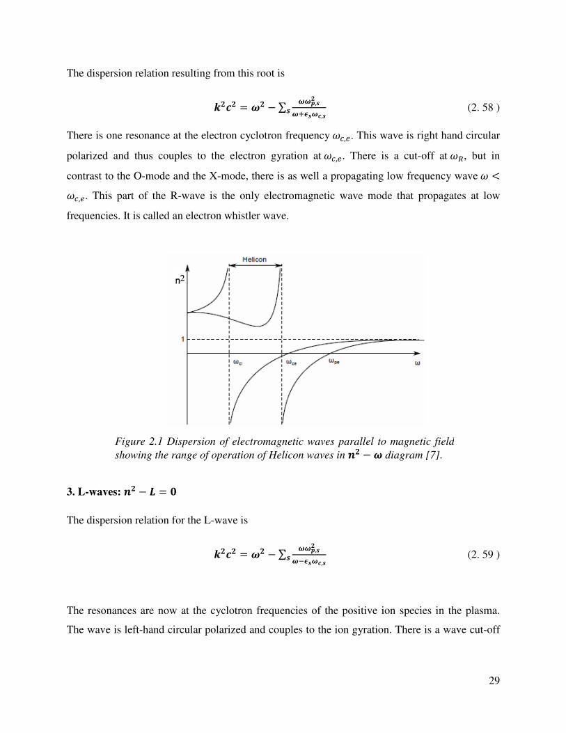
29
The dispersion relation resulting from this root is
C6 = − ∑ ,\¯S\6,\\ (2. 58 )
There is one resonance at the electron cyclotron frequency $%,(. This wave is right hand circular
polarized and thus couples to the electron gyration at $%,(. There is a cut-off at $, but in
contrast to the O-mode and the X-mode, there is as well a propagating low frequency wave $ <$%,(. This part of the R-wave is the only electromagnetic wave mode that propagates at low
frequencies. It is called an electron whistler wave.
3. L-waves: − =
The dispersion relation for the L-wave is
C6 = − ∑ ,\ S\6,\\ (2. 59 )
The resonances are now at the cyclotron frequencies of the positive ion species in the plasma.
The wave is left-hand circular polarized and couples to the ion gyration. There is a wave cut-off
Figure 2.1 Dispersion of electromagnetic waves parallel to magnetic field
showing the range of operation of Helicon waves in − diagram [7].

30
at $«. For frequencies well above the ion cyclotron frequency, the magnetic field has no
influence on the ion motion. Low frequency L waves are called ion whistler waves.
Propagation at Arbitrary Angles:
R-waves in unbounded plasmas do not necessarily have to propagate purely parallel to the
ambient magnetic field. The angle between the wave vector k and the ambient magnetic field B0
is called θ.
The dispersion relation Eq. 2.45 can alternatively expressed as Appleton-Hartree equation [1],
= + ( 3¯)3 ±3 (2. 60 )
Neglecting collision and ion motions for finding out the right circularly polarized high frequency
waves with quasi longitudinal approximation ≈ 0 and $%&,)& ≪ $ < $%( ≪ $)(, the
dispersion relation has the following form
= − (6 ·¸¹ ) (2. 61 )
For the frequency range of interest, ( $%&,)& ≪ $ < $%( ≪ $)() and taking
= %>@ " ncos = %>¾@ the widely used helicon dispersion can be written as the dispersion
relation becomes
= C6 = (6 ·¸¹ ) (2. 62 )
Rearranging this equation in terms of frequency we get,
= 66G\ C6 ¯C6 (2. 63 )
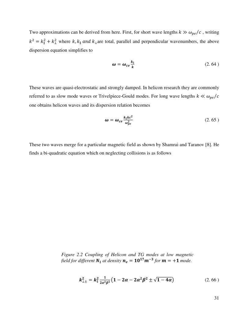
Two approximations can be derived from here. First, for short wave lengthsK = K∥ + K¿ where K, K∥ " Kdispersion equation simplifies to
These waves are quasi-electrostatic and strongly damped. In helicon research they are commonly
referred to as slow mode waves or Trivelpiece
one obtains helicon waves and its dispersion relation becomes
These two waves merge for a particular magnetic field as shown by Shamrai and Taranov [8]. He
finds a bi-quadratic equation which on neglecting collisions is as follows
C¿± =
Figure 2.2 Coupling of Helicon and TG modes at low magnetic
field for different
Two approximations can be derived from here. First, for short wave lengths K ≫K¿are total, parallel and perpendicular wavenumbers, the above
= 6 C∥C
electrostatic and strongly damped. In helicon research they are commonly
referred to as slow mode waves or Trivelpiece-Gould modes. For long wave lengths
one obtains helicon waves and its dispersion relation becomes
= 6 C∥C6
These two waves merge for a particular magnetic field as shown by Shamrai and Taranov [8]. He
quadratic equation which on neglecting collisions is as follows
C∥ ÀÁ c − À − ÀÁ ± √ − Àd
Figure 2.2 Coupling of Helicon and TG modes at low magnetic
field for different ∥ at density = for = + mode.
31
≫ $)( ⁄ , writing
are total, parallel and perpendicular wavenumbers, the above
(2. 64 )
electrostatic and strongly damped. In helicon research they are commonly
Gould modes. For long wave lengths K ≪ $)( ⁄
(2. 65 )
These two waves merge for a particular magnetic field as shown by Shamrai and Taranov [8]. He
d (2. 66 )
Figure 2.2 Coupling of Helicon and TG modes at low magnetic
mode.

The slow wave with K¿ = K¿¯corresponds to the helicon wave. They merge when
solutions in plasmas with density
At low magnetic fields the modes are indistinct and at higher magnetic fields they are very much
apart in perpendicular wave numbers. The TG modes have very short wavelengths and are
confined to the plasma boundary. Figure 2.3 shows the propagation regimes of TG and helicon
modes including the cut-off conditions in the n
2.3 Oblique propagation and Resonance cone
The RCP dispersion can be written again as
Figure 2.3 n-B diagram showing the parameter space of Helicon and TG
modes [8].
À = 6 ∥ , Á = 6∥
¯ corresponds to TG wave and the fast wave with
corresponds to the helicon wave. They merge when à = 1 4⁄ . Figure 2.2 describes the two
solutions in plasmas with density ( = 1 × 10,Ä . and for different parallel refractive indices.
At low magnetic fields the modes are indistinct and at higher magnetic fields they are very much
icular wave numbers. The TG modes have very short wavelengths and are
confined to the plasma boundary. Figure 2.3 shows the propagation regimes of TG and helicon
off conditions in the n-B parameter space [Shamrai et al 1996].
Oblique propagation and Resonance cone
The RCP dispersion can be written again as
B diagram showing the parameter space of Helicon and TG
32
(2. 67 )
corresponds to TG wave and the fast wave with K¿ = K¿
Figure 2.2 describes the two
and for different parallel refractive indices.
At low magnetic fields the modes are indistinct and at higher magnetic fields they are very much
icular wave numbers. The TG modes have very short wavelengths and are
confined to the plasma boundary. Figure 2.3 shows the propagation regimes of TG and helicon
B parameter space [Shamrai et al 1996].
B diagram showing the parameter space of Helicon and TG

Where is the angle between wave propagation direction and the magnetic field,
The refractive index has a resonance for [1]
and N(e is known as the resonance cone angle. When a wave propagates at an angle
the wave number becomes infinitely large. The potential of a point source at the cone apex is
given by [1, 9-10]
Figure 2.4 Resonance cone showing the infinite potential surface of a
point source at cone apex.
= $)($($%( − $)
is the angle between wave propagation direction and the magnetic field,
The refractive index has a resonance for [1]
= \ = 6G\ 6
is known as the resonance cone angle. When a wave propagates at an angle
the wave number becomes infinitely large. The potential of a point source at the cone apex is
Å(, k)~ [ÇSx ¯k y È
Figure 2.4 Resonance cone showing the infinite potential surface of a
point source at cone apex.
33
is the angle between wave propagation direction and the magnetic field, Kl = K cos .
(2. 68 )
is known as the resonance cone angle. When a wave propagates at an angle = N(e ,
the wave number becomes infinitely large. The potential of a point source at the cone apex is
(2. 69 )
Figure 2.4 Resonance cone showing the infinite potential surface of a

34
, where S and P are the Stix coefficients. # and are the radial and axial directions of the cone
and the potential diverges for resonance cone angle tan N(e = # ⁄ = ±− £ ⁄ . As the cold
plasma in principle can have large wave numbers, the wave electric field increases near the
resonance cone boundary [1, 11]. Thermal effects come into effect when wave number K
becomes so large that the wave phase velocity becomes smaller than the thermal speed of the
particles. Fisher and Gould first observed the resonance cones [9] and the thermal effects [10]
where they have found that the potential near the resonance cone boundary is large but finite.
2.4 Helicon waves in a cylinder
So far, we have described plasma waves that propagate in an unbounded medium. Now we will
address bounded helicon waves. In the previous section the dispersion relation is derived which
has two solutions namely the TG mode and Helicon mode. There in equation 2.36, the values of
the parallel and perpendicular wavenumbers are continuous as also evident from Figure 2.2. But
when the wave is bounded in either a conducting or dielectric boundary we will see that the wave
numbers are discrete and quantized. Taking ions immobile and neglecting collisions in a cold
plasma the generalized Ohm’s law (Equation 2.40) gives the current W for an applied electric and
magnetic field.
2 = [ U × 3 + [4U45 (2. 70 )
Taking the curl of the above equation, using the Maxwell’s equation and looking for harmonic
solutions in space and time
3 = C3[ U − [ 0 × U (2. 71 )
Ignoring the displacement current [2] and rearranging
ËÌ × (Ì × 3) − CÌ × 3 + ËC\3 = (2. 72 )

35
Where Í = $ $%(⁄ , and Ke = $)( ⁄ . Equation 2.40 can be factorized as
(0 × −C¿¯)(0 × −C¿ )3 = (2. 73 )
Here K¿¯and K¿ are perpendicular wave numbers for a given axial wave number. The general
solution is the sum of individual solutions [2]
9 = 9¯ + 9 (2. 74 )
where 0 × 3¯ = C¿¯3¯ (2. 75 )
0 × 3 = C¿ 3 (2. 76 )
The helicon dispersion relation can still be obtained from equation 2.40 by letting $ ≪ $%( i.e.
0 × 3 = C¿3 (2. 77 )
As wave magnetic field components are directly measurable quantities with a B-dot probe, a
solution for them is sought. The general behavior of equations 2.75 and 2.76 can be equation
2.77. Taking the curl of this equation gives
03 = C¿ 3 (2. 78 )
Now assuming a harmonic solution in a cylindrical coordinate system (#, , ) like 9, : =9;, :;<&(Îϯ>¾l @A), the solution for z component of 9 is
3k = U(C¿) + 3Ð(C¿) (2. 79 )

36
Where WÎ is the Bessel function of first kind. A and B are arbitrary constants. ÑÎ is Bessel
function of second kind. ÑÎ(#) diverges at r =0 giving B=0.
So
3k = U(C¿) (2. 80 )
Similarly the other components of 9 can be written as [Klozenberg 1968, Chen 1991]
3 = hCÒ ³(C + Ck)U (C¿) + (C − Ck)U¯(C¿)´ (2. 81 )
Figure 2.5 Mode structure of m=0, +1 modes in a plasma with cylindrical boundary.
37
3 = − hCÒ ³(C + Ck)U (C¿) − (C − Ck)U¯(C¿)´ (2. 82 )
And the electric field components are obtained using the Faraday’s law by putting the 9
components.
2k = (2. 83 )
2 = C 3 (2. 84 )
2 = − C 3 (2. 85 )
The boundary condition is same for either a conducting or a dielectric boundary [12]
requiring 9N(#)|NÔ = 0. This lead to the boundary condition as [12]
CkU(C¿) + CCkUÕ (C¿) = (2. 86 )
Where the prime denotes first order derivative with respect to the radial coordinate. Equation
2.65 and the boundary condition equation 2.86 together can be used for a known density and
magnetic field to find out the two unknowns as K¿ and K∥.
2.5 Helicon mode structure in non uniform radial density
All the above calculations for helicon dispersion and mode structure are calculated for a uniform
radial density profile. The effects of realistic non-uniform density profile are on both dispersion
and mode structures. Aliev and Kramer [13] have shown that for a parabolic radial density
profile, the dispersion is $ Ã K, compared to $ Ã K. Though the theory suggests for a uniform
plasma $ Ã K, experiments by Degeling et al [14] have found a quadratic scaling of frequency
with wave number. Results of effect of peaked density profiles show that m= -1 modes cannot
propagate in a highly non-uniform plasma cylinder. So m= +1 modes can be used to produce less
dense plasma with high radial uniformity and m=-1 modes can be used to produce sharper radial

38
profile with dense plasma at centre. M.P. Reilly [15] and Chen et al [16] have calculated the
mode structures numerically for different radial density profiles and has found that the wave field
profiles get more shrunken in radius with sharper density profiles.
2.6 Models of Helicon Power Deposition
Though rigorous theory and experiment has been performed in Helicon physics and helicon
discharges, the high efficiency of the helicon waves is still under study. At least five different
directions have been tried by many helicon physicists will be briefly outlined below.
Chen [12] has calculated the damping rate of Helicon waves through wave particle interaction
(landau damping) and has shown that the damping rates can explain the efficient ionization in
helicon sources. Molvik [17] has used a high acceptance angle retarding field energy analyzer
and observed electron beams in the helicon sources. These results are consistent with results by
Ellingboe et al [1995] who have observed phased light emissions from the plasma. Later
Blackwell and Chen [18] have shown that the number of fast electrons is very few to explain the
Landau damping mechanism. An analytical calculation by Chen et al [19] further estimated the
upper limit of Landau damping in a helicon discharge.
Shamrai et al. [8] have proposed that the efficiency of the absorption mechanism is not due to
Landau damping, as proposed by Chen [12], but to coupling to quasielectrostatic Trivelpiece-
Gould modes, which are rapidly absorbed as they propagate inward from the radial boundary.
Efficiency in power coupling to plasma by Trivelpiece-Gould modes is numerically shown to be
higher than the helicon waves by Borg and Boswell [20], Arnush [2000], Shamrai and Taranov
[8] and Shamrai and Shinohara [21]. Aliev and Kramer [22] have shown that for peaked radial
density profile the mode conversion from the helicon to TG mode is possible at lower densities
because of the modification of the wave mode structure by non-uniform radial density profiles.
Direct measurement of TG modes is difficult because these modes are localized near the plasma
boundary and also they have very short wavelengths in ~1 mm. However, Blackwell et al [23]
have measured the high frequency current profile with WÖ probes to find evidence of TG modes in
a low field helicon discharge but there is no direct measurement so far of these short waves.

39
Akhiezer et al [24] first theoretically proposed a non linear mechanism by which short scale ion
acoustic turbulence excited through a kinetic parametric process causes strong absorption of
helicon waves. Later Kramer et al [25] showed experimentally by cross correlation techniques
using electric probes and microwave back-scattering that helicon wave decays into a TG waves
travelling from boundary to inner plasma and ion acoustic fluctuations travelling from core to
boundary. These ion acoustic fluctuations are correlated with the strong absorption of helicon
waves. Lorentz et al [26] later found the threshold for parametric process and also the
frequencies of pump and decay waves along with wave numbering parallel and perpendicular to
magnetic field all obey the parametric decay process.
Degeling et al [14, 27] have shown both numerically and experimentally that the electrons in a
Maxwellian distribution with velocities slower than the wave get trapped in the longitudinal
component of the helicon wave electric field and are accelerated taking energy from the wave. It
is shown in this work that electrons in a 3 eV Maxwellian distribution can have high enough
energy to be near the maximum of Argon ionization cross section. The outcome of this model i.e.
ionization pulses will travel away from the source at the wave phase velocity has been proved
experimentally by Ellingboe et al [28] by measuring the Ar+ light emission pulses at RF period
by time resolved optical emission spectroscopy within a tenth of RF period.
Briezman and Arifiev [29] have shown analytical calculations for non-axisymmetric modes
(|| = 1) for small longitudinal wave numbers with $ Ã Kl that radially localized surface wave
type helicon modes which are decoupled from the TG modes can be excited in a radially non-
uniform plasma, which can deposit energy through the process of wave particle interaction
(Landau damping). With their lower wave frequency compared to normal helicons, the Landau
damping rates are higher than normal helicons in uniform plasmas. Experimental radial density
profile is used by Chen et al [30] to show RLH mode excitation and power deposition with
frequencies close to the exciter frequency.
2.7 Mode Transitions in Helicon Discharge
Mode transitions are studied in RF capacitive, inductive and Helicon plasmas. In case of a RF
capacitive plasma the discharge changes from a low density à discharge to a high density ×
discharge by increasing the RF voltage [31-32]. It is shown that the transition happens when the

40
ionisation by the electrons emitted by secondary emissions is equal to the ionisation by the bulk
electrons bouncing between the sheaths of the capacitive discharge plates.
In case of Inductive discharges the discharge is maintained by the induced electric fields
produced by the antenna currents. This inductive electric fields drive plasma currents in order to
oppose the magnetic fields produced by the antenna currents. At low density the plasma is
maintained by capacitive electric fields as the skin depth is more so that the RF electric fields
produced by the antenna high voltage can couple directly. But as the density is increased, the
skin depth decreases and the electromagnetic fields decay exponentially within a very thin layer
of plasma. This is the reason an inductive discharge is characterized by a hollow radial density
profile. Also the RF electric field modulation of the plasma potential is much less compared to
capacitive discharges. Capacitive and inductive discharges do not need an external magnetic
field.
When an external magnetic field is applied to plasma, the dielectric of the plasma changes and
can have normal modes which are of electromagnetic in nature. So, magnetized plasma allows
certain frequencies depending upon parameters such as density and magnetic field for
electromagnetic wave to penetrate to the core of the plasma. The electric field of these
electromagnetic waves can deposit energy through either collisional or collisional processes.
ECR and helicon sources are good example of wave sustained discharges but helicon can operate
in all the three discharge regimes depending upon the density which can be increased either by
RF power or magnetic field [33].

41
2.8 Summary of the Chapter
Cold plasma dielectric tensor is derived from equation of motion and Maxwell’s
equation. Solutions for parallel to magnetic field propagation suggest longitudinal plasma
oscillations along with transverse electron and ion cyclotron waves. Whistler dispersion relation
and its bounded version as helicon wave dispersion relation are derived. Resonance cone
propagation of right polarized waves is discussed in the context of quasiparallel wave
propagation. Helicon wave field structure is calculated from generalized Ohm’s law and
Maxwell’s equations. Finite electron mass effect is shown to give another solution as
quasielectrostatic TG modes along with the normal quasielectromagnetic helicon modes. Helicon
radial magnetic field profile for m=0 and m=1 modes are presented pictorially. Different
coupling mechanisms to plasma by helicon waves are discussed. Mode transition in RF
discharges is explained for capacitive, inductive and helicon discharges.
Figure 2.6 Mode transition in a helicon discharge by changing magnetic field [33].

42
References
[1] Paul Murray Bellan. (2006). Fundamentals of plasma physics. Cambridge University Press.
[2] J. P. Klozenberg, B. McNamara, and P. C. Thonemann, “The dispersion and attenuation of helicon waves in a uniform cylidrical plasma,” Journal of Fluid Mechanics, vol. 21, pp. 545-563, 1965.
[3] Blevin, H. A., and P. J. Christiansen. "Helicon waves in a non-uniform plasma." Plasma
Physics 10, no. 8 (1968): 799.
[4] Ferrari, R. L., and J. P. Klozenberg. "The dispersion and attenuation of helicon waves in a cylindrical plasma-filled wave-guide." Journal of Plasma Physics 2, no. 02 (1968): 283-289.
[5] T. H. Stix, The Theory of Plasma Waves: McGraw-Hill, 1962.
[6] Swanson, D. G. "Plasma waves” Academic Press, Boston, MA (USA), 1989.
[7]Boswell, Rod W., and Francis F. Chen. "Helicons-the early years." Plasma Science, IEEE
Transactions on 25, no. 6 (1997): 1229-1244.
[8] Shamrai, Konstantin P., and Vladimir B. Taranov. "Volume and surface rf power absorption in a helicon plasma source." Plasma Sources Science and Technology 5.3 (1996): 474.
[9] Fisher, R. K., and Gould, R. W. (1969). Resonance cones in the field pattern of a short antenna in an anisotropic plasma. Physical Review Letters, 22(21), 1093.
[10] Fisher, R. K., and Gould, R. W. (1971). Resonance cones in the field pattern of a radio frequency probe in a warm anisotropic plasma. Physics of Fluids, 14, 857.
[11] Kuehl, H. H. (1974). Electric field and potential near the plasma resonance cone. Physics of
Fluids, 17, 1275.
[12] F. F. Chen, “Plasma Ionization by Helicon Waves,” Plasma Physics and Controlled Fusion, vol. 33, no. 4, pp. 26, 1991.
[13] Aliev, Yu M., and M. Kramer. "Effect of the plasma density gradient on helicon mode dispersion." Physica Scripta 79.3 (2009): 035502.
[14] Degeling, A. W., C. O. Jung, R. W. Boswell, and A. R. Ellingboe. "Plasma production from helicon waves." Physics of Plasmas 3 (1996): 2788.
[15] Reilly, Michael P. Thesis Three Dimensional Imaging of Helicon Wave Fields via Magnetic
Induction Probes (2009).

43
[16] Chen, Francis F., M. Johannes Hsieh, and Max Light. "Helicon waves in a non-uniform plasma." Plasma Sources Science and Technology 3, no. 1 (1994): 49.
[17] Molvik, A. W., A. R. Ellingboe, and T. D. Rognlien. "Hot-electron production and wave structure in a helicon plasma source." Physical Review Letters 79.2 (1997): 233.
[18] Blackwell, David D., and Francis F. Chen. "Time-resolved measurements of the electron energy distribution function in a helicon plasma." Plasma Sources Science and Technology 10.2 (2001): 226.
[19] F. F. Chen, and D. D. Blackwell, “Upper Limit to Landau Damping in Helicon Discharges,” Physical Review Letters, vol. 82, no. 13, pp. 2677, 1999.
[20] Borg, G. G., and R. W. Boswell. "Power coupling to helicon and Trivelpiece–Gould modes in helicon sources." Physics of Plasmas 5 (1998): 564.
[21] Shamrai, Konstantin P., and Shunjiro Shinohara. "Spectral and spatial characterization of a radio frequency power absorption in high pressure helicon plasmas." Physics of Plasmas 8 (2001): 4659.
[22] Aliev, Yu M., and M. Krämer. "Mode conversion of nonaxisymmetric modes in strongly nonuniform helicon-sustained plasma." Physics of Plasmas 15 (2008): 104502.
[23] Blackwell, D. D., T. G. Madziwa, D. Arnush, and F. F. Chen. "Evidence for Trivelpiece-Gould modes in a helicon discharge." Physical review letters 88, no. 14 (2002): 145002-145002.
[24] Akhiezer, A. I., Mikhailenko, V. S., and Stepanov, K. N. (1998). Ion-sound parametric turbulence and anomalous electron heating with application to helicon plasma sources. Physics
Letters A, 245(1), 117-122.
[25] Krämer, M., Aliev, Y. M., Altukhov, A. B., Gurchenko, A. D., Gusakov, E. Z., and Niemi, K. (2007). Anomalous helicon wave absorption and parametric excitation of electrostatic fluctuations in a helicon-produced plasma. Plasma Physics and Controlled Fusion, 49(5A), A167.
[26] Lorenz, B., Krämer, M., Selenin, V. L., and Aliev, Y. M. (2005). Excitation of short-scale fluctuations by parametric decay of helicon waves into ion–sound and Trivelpiece–Gould waves. Plasma Sources Science and Technology, 14(3), 623.
[27] Degeling, A. W., and R. W. Boswell. "Modeling ionization by helicon waves." Physics of
Plasmas 4 (1997): 2748.
[28] Ellingboe, A. R., R. W. Boswell, J. P. Booth, and N. Sadeghi. "Electron beam pulses produced by helicon‐wave excitation." Physics of Plasmas 2 (1995): 1807.
[29] B. N. Breizman, and A. V. Arefiev, “Radially Localized Helicon Modes in Nonuniform Plasma,” Physical Review Letters, vol. 84, no. 17, pp. 4, 2000.
44
[30] Chen, Guangye, Alexey V. Arefiev, Roger D. Bengtson, Boris N. Breizman, Charles A. Lee, and Laxminarayan L. Raja. "Resonant power absorption in helicon plasma sources." Physics of plasmas 13 (2006): 123507.
[31] Odrobina, I., and Kando, M. Discontinuous transitions between alpha and gamma regimes of rf capacitive discharge. Plasma Sources Science and Technology, 5, 517 (1996).
[32] Moon, Se Youn, J. K. Rhee, Dan Bee Kim, and Wonho Choe. "α, γ, and normal, abnormal glow discharge modes in radio-frequency capacitively coupled discharges at atmospheric pressure." Physics of Plasmas 13 (2006): 033502.
[33] Boswell, R. W. "Very efficient plasma generation by whistler waves near the lower hybrid frequency." Plasma Physics and Controlled Fusion 26.10 (1984): 1147.

45
Chapter 3
Experimental Set up and Diagnostics
3.1 Introduction
The experimental works presented in this thesis are performed in a linear magnetized plasma
device (Figure 3.1) produced by RF electric fields. The magnetic field is produced by a set of
water cooled electromagnets arranged to give a uniform magnetic field in the source chamber.
The RF antenna powered by a 2.5 kW RF generator along with an L-type matching network
produces the plasma. The antenna is installed around a cylindrical glass tube connected to a
cylindrical vessel made of SS304. This chapter describes the apparatus and diagnostics. The
apparatus can be divided into three main sections: the vacuum system, the electromagnets and
the RF system. The RF system consists of half helical helicon antenna, RF power source,
matching network and RF shielding and grounding. Diagnostics used are various Langmuir
probes for density, temperature and floating potential measurements, emissive probe for plasma
potential measurement, magnetic probe for measuring wave field amplitude and phase,
Rogowski for antenna current measurements.
3.2 Vacuum Vessel and Vacuum System
The total length of the experimental chamber is approximately 120 cm, which comprises
of two linear chambers of cylindrical cross section of different radii, as shown in Figure 3.2. The
first chamber, called the source chamber hereafter, measures 70 cm in length and is made up of
borosilicate glass tube of 10 cm diameter with wall thickness of 0.4 cm. The RF antenna is
installed around this cylindrical glass tube. One end of this glass tube is closed with an insulated
end flange to make the plasma system current free and the other end is connected to a cylindrical
diffusion chamber made up of stainless steel having an inner diameter of 21 cm and length of 50

46
cm. As the plasma diffuses to this chamber from the source chamber it is called the diffusion
chamber. A stainless steel metal flange closes the other end of the diffusion chamber.
The plasma is produced in the source chamber and has four orthogonal diagnostic ports for
diagnosing the source chamber plasma. The diffusion chamber has 15 radial ports on its
periphery and three ports on the diffusion chamber end flange for various diagnostics.
Figure 3.1 Picture of Helicon experimental Set up.
Figure 3.2 Schematic of the helicon experimental set up.
47
The vacuum chamber is Helium leak tested up to 1 x 10⁻⁷ mbar-liter/sec. A 1000 liter/s diffusion
pump backed by a rotary pump is used to evacuate the system up to a minimum base pressure of
1 x 10⁻⁶ mbar. The pressure is measured in the diffusion chamber by an Alcatel Vacuum make
AHC 2000, hot cathode-crystal combo gauge. The operational or fill-in pressure is varied from 1
x 10-4 mbar to 5 x 10⁻³ mbar. Gas is filled through a Pfeiffer make gas-dosing valve connected to
the end flange of the source chamber, which allows fine changes in the system neutral gas
pressure. Argon gas is used most of the times unless otherwise stated.
3.3 Electromagnets
The axial magnetic field is created by seven electromagnets made up of hollow copper
pipes of 0.6 cm inner diameter and 0.8 cm outer diameter. The hollow pipes facilitate forced
water flow to cool the electromagnets at high current for steady state operation. These tubes are
wound over a PVC pipe of 33 cm outer diameter and with wall thickness 0.4 cm, which is
supported on both sides by rectangular hylam blocks (60 cm x 60 cm) of 1.6 cm thickness. The
inner diameter of each coil is 31.5 cm and the height and width are 6 cm each. Self-adhesive
cotton tape of 500 micron thickness is used to achieve layer to layer insulation up to 1.5 kV. In
each coil there are six layers each having six turns totaling 36 turns. Each magnet has a
resistance of ~ 40 mili-Ohms. These magnets are then placed on an aluminum stand with proper
mechanical support to withstand the electromagnetic forces acting on them. The placement of the
magnets is shown in Figure 3.2. The magnets are aligned very carefully to make axis of magnets
collinear with the vacuum vessel. A Sorensen make variable power supply rated 60 V, 167 A is
used to power the electromagnets to achieve a maximum magnetic field of ~ 400 Gauss. Before
mounting the electromagnets, each of them is separately tested for water flow, magnetic field and
resistance. After assembling the magnets, a current of 52.5 Amp is passed through six magnets
(as shown in Figure 3.2 excluding the seventh coil) connected in series and the magnetic field
value on the axis of the chamber using is measured using a H.W. BELL Hall probe. The
magnetic field is also simulated with EFFI code [1] by using the real coil dimensions such as
average coil diameter, width, height and current density. Figure 3.3(a) shows the simulated and
the measured axial magnetic field values along the axis of the chamber with six magnets. The
measured magnetic field matches very well with the simulated values. To achieve different
gradients in the axial direction we simulated the axial magnetic field profile with all the seven

48
magnets by varying the current in the seventh coil. Figure 3.3(b) clearly shows that several
different gradients of magnetic field in the axial direction can be achieved in the machine
varying the current in the seventh coil.
Figure 3.3 (a)Plot for magnetic field produced by 6 magnets at -47.8, -38.5, -
20,-3.5, 13, 30 by passing a positive current of 52 Ampere and (b) additional
variable current in the seventh coil at 47 cm to get a variable gradient.

49
Table 3.1 Parameter regime, length scales and time scales of the present helicon experiment.
3.4 Antenna and RF Matching Circuit
As the half wavelength antenna is shown to be more efficient [2] compared to the full
wavelength antenna, we have designed and fabricated a half-wavelength helical m = +1 antenna
with diameter of 12 cm and length of 18 cm. Picture of this antenna is shown in Figure 3.4. The
antenna is connected to matching network through a shielded twin coaxial transmission line of
diameter 3.5 cm. The helicon antenna is placed around the source (glass) chamber and RF
shielding of the antenna is done by putting a 2 mm thick hollow coaxial copper cylinder of 20 cm
Parameter (Unit) Values for Argon gas
B (Gauss) 1-400
P neutral (mbar) 4 x 10⁻³ – 1 x 10⁻⁴
n (1011 cm-3) 0.1 - 5
Te (eV) 3 - 8
λ Debye (cm) 1.8 x10⁻³- 2.1 x 10⁻²
re (cm) 0.01 - 10
ri (cm) 1 - 460
fpe (GHz) 0.87 – 6.28
fce (MHz) 2.8 – 1105
fci (kHz) 0.37 – 15
fe-n (kHz) 50 - 3267
fi-n (kHz) 0.466 - 30

50
inner diameter and 25 cm length around it. The remaining part of the glass chamber is covered
by two layers of brass mesh of 30% transparency. The full grounding and shielding scheme is
elaborated in Figure 3.2. Proper RF shielding is ensured by measuring the radiation fields outside
the antenna region by a Narda make field meter and is found to be less than 5 V/m in 1 meter
radius from the antenna. A 13.56 MHz Advance Energy make MOSFET based RF amplifier is
used to power the antenna. The amplifier has characteristic output impedance of 50 Ohm and it
can supply RF power up to 2.5 kW with maximum reflection of 400 W. It contains an inbuilt
power meter, which displays the forward and the reflected power.
The matching network used is a CESAR make 5 kW capacitive L-matching network designed
for an inductive load [3]. The picture of the matching network is shown in Figure 3.4. There exist
Figure 3.4 Picture of the inside of the match box showing the
variable Load and Tune Capacitors with auxiliary inductors.

51
two variable capacitors in the matching network, one is a load capacitor (CL), which can be tuned
from 20 to 1000 pF and another is a tune capacitor (CT), which can be tuned from 5 to 500 pF.
3.4.1 The Antenna
Various antennas are used to produce helicon plasma [4]. A right half helical antenna is
used for the present work. The helical antenna consists of two helical windings wound around
the outside of the glass tube each azimuthally 180 degree displaced. Antenna is placed on two
teflon spacers of about 3mm thick at the antenna ends fixed from the outside of the glass tube.
The current in each winding is in the opposite direction to each other. This antenna is constructed
with one length of copper plate with the two winding joined by a half loop at one end as shown
in Figure 3.5. The helical antenna has a higher selectivity of parallel wavelength [5] than the
double saddle coil [6] thus decreasing its useful wavelength range. For present experiment the
length of the antenna chosen is 18 cm.
Figure 3.5 Picture of the half helical m=+1 antenna just before installation.

3.4.2 Matching Network
To ensure that the transmission line from the RF transmitter is terminated at its
characteristics impedance the antenna is incorporated into an L
predominantly behaves like an inductor as shown in Figure 3.5. When there is no pla
resistance is the electrical resistance of the antenna. Once plasma is formed the resistance will
increase. The output impedance (50
antenna-plasma load for maximum power transfer. We used a comme
network (AE, VM 5000 W) with a tuning unit. The tuning unit contains the matching
components (variable capacitors and inductors), two dc motor servos, and RF sensors to provide
feedback to the dc motor servos. L
variable capacitors. Original capacitors initially provided by the vendor were not enough to
match the impedance of the plasma under variety of experimental conditions. So we opted for a
set of inductors in series with the c
requirement. To have the confidence on the matching network a rough calculation has been
made.
Figure 3.6 Schematic of the matching network attached to RF generator and
a load composed of the a
To ensure that the transmission line from the RF transmitter is terminated at its
characteristics impedance the antenna is incorporated into an L-network, where the antenna
predominantly behaves like an inductor as shown in Figure 3.5. When there is no pla
resistance is the electrical resistance of the antenna. Once plasma is formed the resistance will
increase. The output impedance (50 Ω) of the RF source was matched to the impedance of
plasma load for maximum power transfer. We used a commercial impedance matching
network (AE, VM 5000 W) with a tuning unit. The tuning unit contains the matching
components (variable capacitors and inductors), two dc motor servos, and RF sensors to provide
feedback to the dc motor servos. L-type matching network is employed with two vacuum
variable capacitors. Original capacitors initially provided by the vendor were not enough to
match the impedance of the plasma under variety of experimental conditions. So we opted for a
set of inductors in series with the capacitors and used different inductors as per experimental
requirement. To have the confidence on the matching network a rough calculation has been
Figure 3.6 Schematic of the matching network attached to RF generator and
a load composed of the antenna and plasma.
52
To ensure that the transmission line from the RF transmitter is terminated at its
network, where the antenna
predominantly behaves like an inductor as shown in Figure 3.5. When there is no plasma the
resistance is the electrical resistance of the antenna. Once plasma is formed the resistance will
) of the RF source was matched to the impedance of
rcial impedance matching
network (AE, VM 5000 W) with a tuning unit. The tuning unit contains the matching
components (variable capacitors and inductors), two dc motor servos, and RF sensors to provide
rk is employed with two vacuum
variable capacitors. Original capacitors initially provided by the vendor were not enough to
match the impedance of the plasma under variety of experimental conditions. So we opted for a
apacitors and used different inductors as per experimental
requirement. To have the confidence on the matching network a rough calculation has been
Figure 3.6 Schematic of the matching network attached to RF generator and

53
In Figure 3.6 we show the equivalent circuit of the L-type network is shown in which: LA stands
for the antenna inductance, resistance RP is the electrical resistance of the antenna when the
plasma is switched on, which increases when plasma is on. It is necessary to estimate the load
and the tuning capacitance (CL, CT) for better designing of the L-network. Let us group LA, RP
and CT and call them the tune arm. Its impedance is
ØÙ = h + hÙ + (3.1)
that can be written dividing real from imaginary part as
ÚÛ = ÜÝÞ + ßà (3.2)
where, á = − Ù (3. 3)
Now let's assume that the tune capacitance does not completely cancel out the antenna
inductance, and then the load capacitance can balance the net inductive impedance of the tune
arm. The admittance (i.e. the inverse of the impedance) of the tune and load arm can be written
as
âÙ = ¯á − ãä¯á (3.4)
â = h (3.5)
So that the total admittance å of the L-network is given by
â = âÙ + â (3.6)
To find values of CL and CT, a resonance condition (i.e. along the tuning arm we only see real
impedance) is imposed; then the total conductance (i.e. the real part of the admittance) will equal
the inverse of the total line impedance ZT, and the susceptance (i.e. the imaginary part of the
admittance) of the two arms will cancel. These conditions give us, respectively, the following
equations
á = cØÙ − d (3. 7)

54
= áØÙ (3. 8)
For the antenna, plasma and transmission line we are using, it is possible to assume that æç ≫¡è so that equation (3.7) gives
á = ØÙ (3. 8)
Now combining equations (3.8) and (3.9) one can get the formula for the load capacitance
= ØÙ (3. 10)
and substituting equation (3.9) into (3.3) the formula for the tune capacitance is
Ù = ØÙ (3. 11 )
Figure 3.7 Smith Chart showing operational matching regimes of the
current matching network attached to an inductive helicon antenna.

55
Taking a typical case with LA = 500 nH, RP ~ 1 Ohm, ZT=50 Ohm and $ = 85.2 êë and using
Equations (3.10) and (3.11) we get: CL = 1650 pF and CT = 330 pF. Two COMET make vacuum
variable capacitors are used. By adding suitable inductors (water cooled) in series with the
capacitors, the normal operation in a helicon regime of discharge requires values of CL and CT as
~ 700 pF and ~ 100 pF respectively. The matched region with these capacitors and inductors is
shown by the region bordered with the red line in Figure 3.6. The load capacitor (CL) can be
tuned from 20 to 1000 pF and the tune capacitor (CT) can be tuned from 5 to 500 pF so that zero
reflection matching can be done for RP = 0.1 Ohm to 2 Ohm. Both the capacitors are mounted
inside the tuning box, which is made of silver coated copper, so that it acts as a Faraday cage. On
the top side of the tuning box a fan is mounted to ensure cooling for the two capacitors.
Measuring the power coupled into the plasma is very important for defining correctly the plasma
parameters. The antenna radiation resistance is the principle measure of the efficiency of an
antenna.
For a mismatched load both the voltage and current along with their phase measurement are
necessary to estimate the power delivered to the load. However for a matched load with
negligible reflection, antenna will see plasma as a resistive load only. To evaluate this load we
assume that when plasma is on, the resistance of the antenna is given by the resistance of the
antenna plus that of the plasma
Ù = + (3. 87)
The power dissipated by the antenna can be written as [7]
|Ù = ì − (3. 13)
Measuring RA without plasma we find, from the last two equations, a formula for Rp, which is
the load of the antenna-plasma coupling
= ì | − (3. 14)
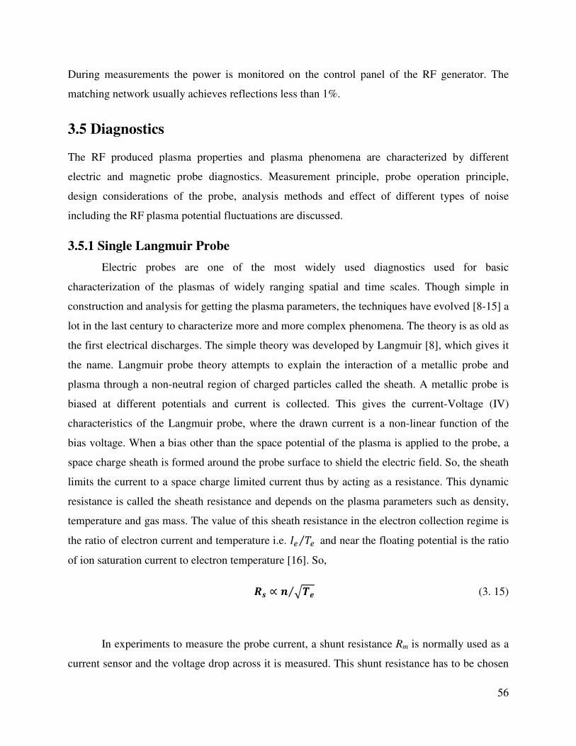
56
During measurements the power is monitored on the control panel of the RF generator. The
matching network usually achieves reflections less than 1%.
3.5 Diagnostics
The RF produced plasma properties and plasma phenomena are characterized by different
electric and magnetic probe diagnostics. Measurement principle, probe operation principle,
design considerations of the probe, analysis methods and effect of different types of noise
including the RF plasma potential fluctuations are discussed.
3.5.1 Single Langmuir Probe
Electric probes are one of the most widely used diagnostics used for basic
characterization of the plasmas of widely ranging spatial and time scales. Though simple in
construction and analysis for getting the plasma parameters, the techniques have evolved [8-15] a
lot in the last century to characterize more and more complex phenomena. The theory is as old as
the first electrical discharges. The simple theory was developed by Langmuir [8], which gives it
the name. Langmuir probe theory attempts to explain the interaction of a metallic probe and
plasma through a non-neutral region of charged particles called the sheath. A metallic probe is
biased at different potentials and current is collected. This gives the current-Voltage (IV)
characteristics of the Langmuir probe, where the drawn current is a non-linear function of the
bias voltage. When a bias other than the space potential of the plasma is applied to the probe, a
space charge sheath is formed around the probe surface to shield the electric field. So, the sheath
limits the current to a space charge limited current thus by acting as a resistance. This dynamic
resistance is called the sheath resistance and depends on the plasma parameters such as density,
temperature and gas mass. The value of this sheath resistance in the electron collection regime is
the ratio of electron current and temperature i.e. í( î( ⁄ and near the floating potential is the ratio
of ion saturation current to electron temperature [16]. So,
\ ∝ Ù⁄ (3. 15)
In experiments to measure the probe current, a shunt resistance Rm is normally used as a
current sensor and the voltage drop across it is measured. This shunt resistance has to be chosen
57
carefully as it becomes a part of the Langmuir probe circuit. In low temperature and low density
plasmas this resistance cannot be very small as then the current signal will be comparable to the
noise level of a practical LP circuit. At the same time to quantify the response of plasma, all the
probe bias voltage should drop in the sheath for which the shunt resistance should not be large
enough that a significant portion of the bias voltage drops across ¡Î only.
In plasma, the electron flux onto a plasma exposed electrically floating probe is more than that of
ions because of mainly two reasons. First, the electrons are lighter than ions and secondly,
random thermal velocity is higher for electrons compared to more or less cold ions. So for a
floating object, the more mobile electrons impinge first. As the probe is electrically floating, the
probe gets charged to a negative potential such that the electrons are repelled and ions are
collected. The potential of the probe settles to a negative potential w.r.t. the plasma potential
such that the fluxes of electron and ion are equal. This equilibrium potential is called the floating
potential of the probe. There are two ways in which the probe current can be made zero or
negligible and the floating potential can be measured. This is done either by changing the bias to
collect negligible current in which case the measuring resistance is much less than sheath
resistance or by removing the bias and making the measuring resistance much higher than the
sheath resistance such that the probe collects a negligible current.
When a probe is biased negative w.r.t. the floating potential an ion rich sheath is formed.
Normally for bias voltages less than four times electron temperature (in volts) less than the
floating potential in Maxwellian plasma, almost all the electrons are repelled and the collected
current in the probe is Bohm current due to ions. This current is called the ion saturation current.
When the probe bias is equal to the space potential of the plasma, then virtually there is
no sheath around the probe as there is no electric field to be shielded. So, all the electrons in the
Maxwellian distribution are collected randomly. This is the maximum electron current and is
known as the electron saturation current to a probe.
When a probe is biased with a potential less than the plasma potential, electrons are
repelled as per their energy. One can scan the entire energy distribution of the electrons just by
varying the probe bias w.r.t the plasma potential. As the bias approaches the floating potential,
only tail electrons in the Maxwellian distribution are collected by the probe and so the current
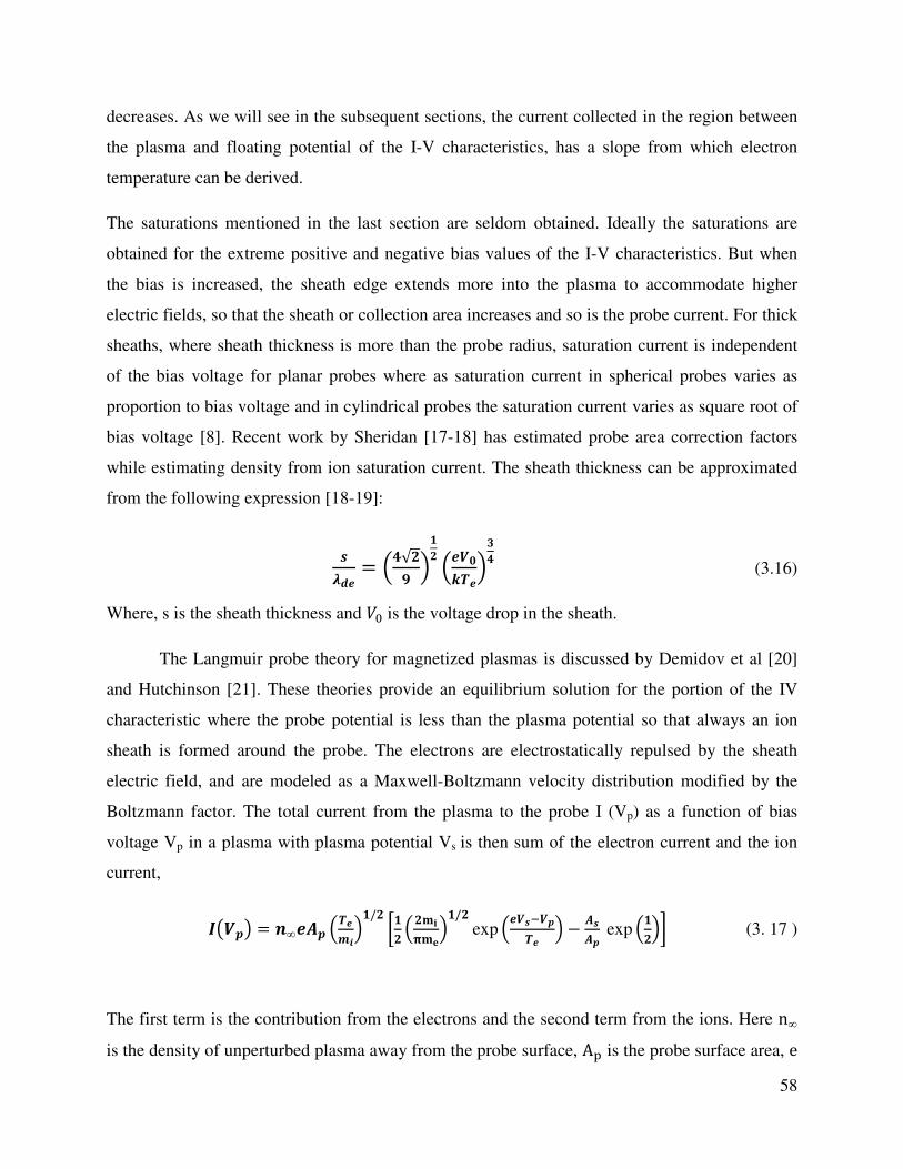
58
decreases. As we will see in the subsequent sections, the current collected in the region between
the plasma and floating potential of the I-V characteristics, has a slope from which electron
temperature can be derived.
The saturations mentioned in the last section are seldom obtained. Ideally the saturations are
obtained for the extreme positive and negative bias values of the I-V characteristics. But when
the bias is increased, the sheath edge extends more into the plasma to accommodate higher
electric fields, so that the sheath or collection area increases and so is the probe current. For thick
sheaths, where sheath thickness is more than the probe radius, saturation current is independent
of the bias voltage for planar probes where as saturation current in spherical probes varies as
proportion to bias voltage and in cylindrical probes the saturation current varies as square root of
bias voltage [8]. Recent work by Sheridan [17-18] has estimated probe area correction factors
while estimating density from ion saturation current. The sheath thickness can be approximated
from the following expression [18-19]:
\ðb = D√ñ E DòCÙE
(3.16)
Where, s is the sheath thickness and ó; is the voltage drop in the sheath.
The Langmuir probe theory for magnetized plasmas is discussed by Demidov et al [20]
and Hutchinson [21]. These theories provide an equilibrium solution for the portion of the IV
characteristic where the probe potential is less than the plasma potential so that always an ion
sheath is formed around the probe. The electrons are electrostatically repulsed by the sheath
electric field, and are modeled as a Maxwell-Boltzmann velocity distribution modified by the
Boltzmann factor. The total current from the plasma to the probe I (Vp) as a function of bias
voltage Vp in a plasma with plasma potential Vs is then sum of the electron current and the ion
current,
|còd = ∞ DÙhE/ ® DôÜõôuE/exp Dò\ òÙ E − \ exp DE° (3. 17 )
The first term is the contribution from the electrons and the second term from the ions. Here n∞
is the density of unperturbed plasma away from the probe surface, A÷ is the probe surface area, e

59
is the electronic charge, mi is ion mass, me is the electron mass, Tú is electron temperature, Aû is
the sheath surface area. A probe diameter can always be chosen such that the radius of the probe
is much larger than the sheath thickness so that the ratio üýüþ is nearly unity. This is called the
planar sheath approximation. Differentiating the probe current w.r.t. the probe bias,
b|bò = Ù (| − |\) + b|\bò (3. 18)
Where Iû is the ion saturation current given by
|\ = exp DE ∞ DÙhE (3. 19)
Assuming, dIû dV ≪ dI dV⁄⁄ , the electron temperature is determined from
Ù = (| |\)b| bò⁄ (3. 20)
Relation between Plasma potential and Floating Potential:
As for the reason described earlier for not getting saturation in a cylindrical probe and also for
high density plasmas like helicon sources one needs to collect a large amount of current to get
the plasma potential, the floating potential where a very less current is collected can give an
estimate of the plasma potential. The floating potential is defined as the potential at which the
probe current goes to zero. The ion flux Γ& to a probe at a potential less than plasma potential is
given by
h = \ DCÙ E (3. 21)
The electron flux Γ( at a bias equal to the floating potential is given by
= \ DCÙÇ E exp DòCÙE (3. 22)
Equating both the fluxes

60
DCÙ E = DCÙÇ E exp DòCÙE (3. 23)
And taking logarithm of both sides we get,
ò = CÙ DÇ E (3. 24)
This is the potential attained by a probe w.r.t. the plasma potential when exposed to plasma and
drawing no current. As the ions are heavier than electrons, a floating probe will always be
charged negative w.r.t. the plasma potential.
For Argon gas used in our experiment V~ − 4.7Tú. Additional -0.5Tú drop in the presheath to
satisfy the Bohm criterion, the plasma potential can be expressed for argon gas as V÷~ V +5.2Tú.
Effect of Magnetic field on Langmuir Probe data analysis:
When a probe is used in plasma with an external magnetic field, the probe current to the
plasma depends on the magnetization of the charged particles. The probe radius has to be
carefully chosen to consider the effect of magnetic field. There are three cases to be considered.
Low magnetic fields: Both electrons and ions have the larmour radius larger than probe radius.
Here the theory of probe collection in unmagnetized case is still applicable. In the intermediate
magnetic fields, the electron larmour radius is smaller than the probe radius but not the ion
larmour radius. In this case the electron current collection in the surface perpendicular to the
magnetic field is reduced. So the ratio of electron and ion saturation current is decreased. We
worked in this regime of magnetic fields. As we are calculating the density from ion saturation
current, the results are unaffected by magnetic field. In case very high magnetic field, both
electron and ion have larmour radius smaller than the probe dimension such that the all the
saturation currents are affected.
Sheath Ionization and its signature:

61
A sheath becomes collisional if the electron-neutral collision length can be
accommodated inside the sheath width. This in our system can happen for a low density high
pressure plasma discharge conditions. When a bias more than the plasma potential is applied, the
electrons before being collected can do an ionizing collision. The lionization leads a secondary
plasma formation near the sheath.
This secondary plasma is sometimes called as an anode double layer and its existence
solely depends on a critical current which in turn depends on the electron number density (which
is more near plasma potential), gas species, collision cross-section and neutral gas pressure. The
IV characteristics instead of being saturated, has a sudden rise in current for incremental increase
of the probe bias above plasma potential. A typical IV characteristics obtained at high pressure
(8x10⁻² mbar) is shown in Figure 3.8.
Probe cleaning:
The probe if not a clean surface can lead to many problems including
erroneous/irreproducible IV characteristics, degassing, secondary emission etc which will
ultimately lead to irreproducible data. Impurities on the probe surface can be cleaned by heating
the surface. This is done by keeping the probe in electron saturation mode for longer times. As
Figure 3.8 Typical IV characteristics of Langmuir probe with
sheath ionization.

62
the magnitude of electron current is more, this will heat the probe surface through Jule heating
and the surface gets cleaned. Some impurities can stick to the surface of the probe which can be
cleaned by bombarding ions on to the probe by keeping the probe in the ion saturation regime.
The ions hit the surface and clean it by sputtering the probe surface.
Probe, probe holder, and shaft Size limitations:
The planar sheath approximation has the basic assumption that the sheath thickness is
smaller than the probe radius. When the sheath thickness is high, large currents can now flow,
the sheath resistance decreases. . The frequency response (∝ 1 ¡e⁄ e) of a Langmuir probe is
inversely proportional to the sheath resistance. So when the sheath resistance decreases with
bigger probe size, the small fluctuations get amplified and affect the DC characteristics. Also a
bigger probe reduces the space resolution. They can also disturb the plasma by taking a large
amount of current. When you have a bigger probe holder which is most of the time an insulator,
it can disturb the plasma electron energy distribution (EEDF). If the rate of loss of high energetic
plasma electrons to the probe holder or shaft is more than the rate of replenishment of these fast
electrons by thermalization processes in the plasma, the EEDF will be significantly affected. The
probe shaft is generally a grounded metallic body which can significantly disturb either by taking
current from the plasma or by disturbing any potential structure if at all to be studied.
Design:
The probe tip is made of 0.5 mm cylindrical tungsten wire with a plasma exposed length
of 3 mm. The probe tip is silver brazed with a copper cable which is connected to a coaxial cable
for signal transfer. The probe tip is inside a ceramic bid and the bid is connected to a machinable
ceramic holder. The probe holder is connected to a SS 304 metallic probe shaft which has
vacuum compatible connection at the other end for both vacuum and electrical integrity. The
probe shaft is housed in a Wilson vacuum feedthru for linear and rotational motion without
breaking the vacuum. A floating source of ±150 V made of batteries in series is used to bias a
high power amplifier (PA-85) which amplifies a triangular ramp signal of ±5 V produced by a
signal generator at a frequency of 1 Hz. This time varying signal is applied to the probe through
a coaxial cable. A shunt resistance of 1 kOhm is used to measure the probe current. The output
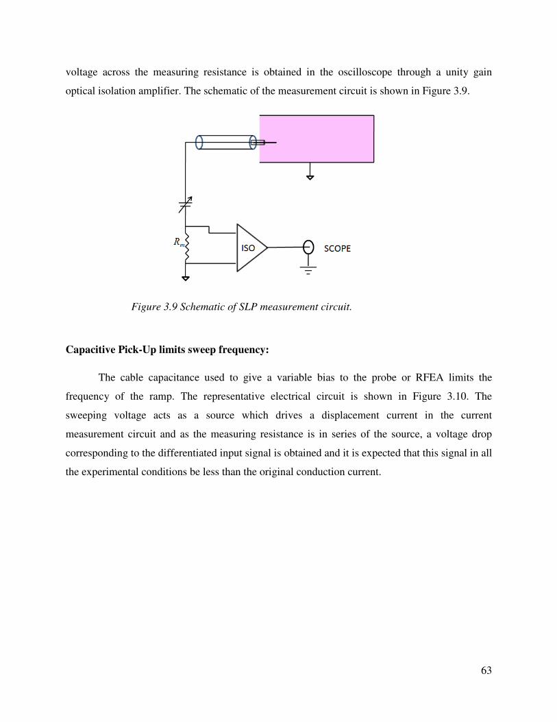
63
voltage across the measuring resistance is obtained in the oscilloscope through a unity gain
optical isolation amplifier. The schematic of the measurement circuit is shown in Figure 3.9.
Capacitive Pick-Up limits sweep frequency:
The cable capacitance used to give a variable bias to the probe or RFEA limits the
frequency of the ramp. The representative electrical circuit is shown in Figure 3.10. The
sweeping voltage acts as a source which drives a displacement current in the current
measurement circuit and as the measuring resistance is in series of the source, a voltage drop
corresponding to the differentiated input signal is obtained and it is expected that this signal in all
the experimental conditions be less than the original conduction current.
Figure 3.9 Schematic of SLP measurement circuit.

64
The output voltage measured across the measuring resistance when there is no plasma is solely
because of the displacement current generated through the stray capacitance of the cable used. So
the voltage drop across the measuring resistance is
ò = |b × (3. 25)
The displacement current can be written as
|b = 4245 = b 4ò45 (3. 26)
Taking V as a sinusoidally varying voltage signal with frequency $ , |b = ò (3. 27)
So the amplitude of voltage drop in the measuring will be
ò = |b × = ò (3. 28)
Figure 3.10 Equivalent electrical circuit of a Langmuir probe for
time varying bias and current measurements.

65
Using a triangular sweep of 70 Vpk-pk, a resistance of 1 k-Ohm and an RG-58 cable of nearly 2
meters, the output voltage across the measuring resistance is plotted with triangular sweep
frequency and is shown in Figure 3.11. It is seen from experiment and calculations; the output
voltage is proportional to frequency. The output characteristic has a form of a square wave as it
should be a differential form of the input signal. This kind of output characteristics in a signal
confirms it to be of capacitive pick up. It should be noted that for low density plasmas, one need
to take care of this sweep frequency, where the generated displacement current can be of the
order of the ion saturation currents.
3.5.2 Wall Probe
When a material body is inserted inside an electron-ion plasma, the floating body is
negatively charged by the electrons. This negative potential is known as the floating potential of
the material and it accelerates the less mobile ions so that the total current to the floating object is
zero. This floating potential depends on electron temperature and electron to ion mass ratio and
is expressed as (Equation 3.24)
ó = 12 Kî(< ln x2ê y,
Figure 3.11 Voltage drop across a measuring resistance in the absence of plasma for
different bias frequencies applied to Langmuir probe through a RG 58 coaxial cable
of 2 meter length showing the limitations of bias frequency.

66
Where, K, î( , and ê are the Boltzmann’s constant, electron temperature, electron mass and ion
mass respectively. As ≪ ê, ó is always negative with respect to the plasma potential.
When a high frequency voltage is applied by a metallic antenna on the outer wall of a
dielectric glass tube, a potential is induced in the inner wall of the glass tube through the
capacitance of the glass which is exposed to the plasma. The plasma electrons respond quickly
compared to the heavier ions. This creates an imbalance in the currents flowing to the dielectric
body and the electrons have to charge the body to a negative potential such that the electron and
ion currents are equal to maintain the floatingness of the dielectric glass wall. This can also be
understood as the rectification of the RF potential by the sheath which has a nonlinear IV
characteristic. For a dielectric wall this process was first explained by Kino and Butler [22].
Figure 3.12 shows how a sheath generates a DC potential and subsequently charges the wall.
This potential is sum of the floating potential of a DC plasma system as described earlier
and another potential because of additional different response of electrons and ions to the high
frequency oscillating electric field. This potential is known as the DC self bias and the total
potential is expressed as per Chabert [23] as
òì = CÙ DÇ E − | DòCÙE (3. 29)
Where I0 is the zero-order modified Bessel function and for sufficiently low RF applied
voltages compared to temperature, its value tends to unity, so that the contribution to floating
potential from the RF can be neglected.
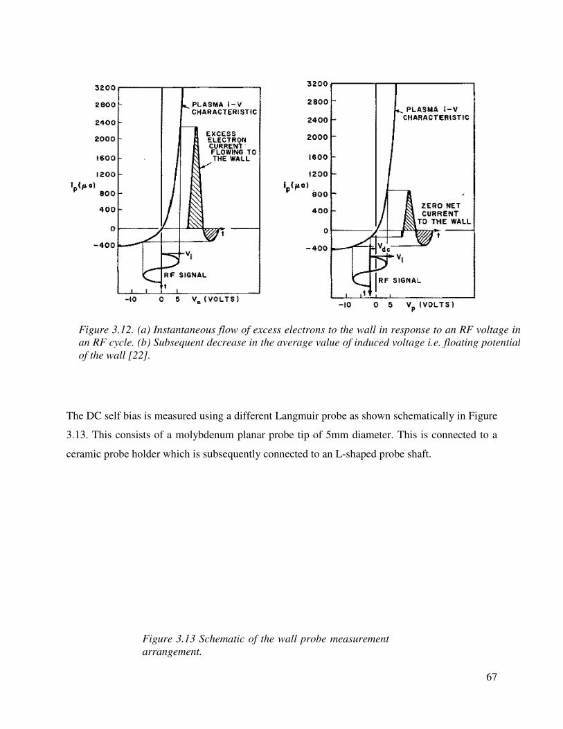
The DC self bias is measured using a different Langmuir probe as sh
3.13. This consists of a molybdenum planar probe tip of 5mm diameter. This is connected to a
ceramic probe holder which is subsequently connected to an L
Figure 3.12. (a) Instantaneous f
an RF cycle. (b) Subsequent decrease in the average value of induced voltage i.e. floating potential
of the wall [22].
Figure 3.13 Schematic of the wall probe measurement
arrangement.
The DC self bias is measured using a different Langmuir probe as shown schematically in Figure
3.13. This consists of a molybdenum planar probe tip of 5mm diameter. This is connected to a
ceramic probe holder which is subsequently connected to an L-shaped probe shaft.
a) Instantaneous flow of excess electrons to the wall in response to an RF voltage in
b) Subsequent decrease in the average value of induced voltage i.e. floating potential
Schematic of the wall probe measurement
67
own schematically in Figure
3.13. This consists of a molybdenum planar probe tip of 5mm diameter. This is connected to a
shaped probe shaft.
low of excess electrons to the wall in response to an RF voltage in
b) Subsequent decrease in the average value of induced voltage i.e. floating potential
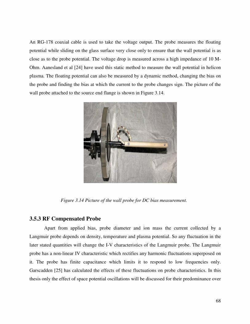
68
An RG-178 coaxial cable is used to take the voltage output. The probe measures the floating
potential while sliding on the glass surface very close only to ensure that the wall potential is as
close as to the probe potential. The voltage drop is measured across a high impedance of 10 M-
Ohm. Aanesland et al [24] have used this static method to measure the wall potential in helicon
plasma. The floating potential can also be measured by a dynamic method, changing the bias on
the probe and finding the bias at which the current to the probe changes sign. The picture of the
wall probe attached to the source end flange is shown in Figure 3.14.
3.5.3 RF Compensated Probe
Apart from applied bias, probe diameter and ion mass the current collected by a
Langmuir probe depends on density, temperature and plasma potential. So any fluctuation in the
later stated quantities will change the I-V characteristics of the Langmuir probe. The Langmuir
probe has a non-linear IV characteristic which rectifies any harmonic fluctuations superposed on
it. The probe has finite capacitance which limits it to respond to low frequencies only.
Garscadden [25] has calculated the effects of these fluctuations on probe characteristics. In this
thesis only the effect of space potential oscillations will be discussed for their predominance over
Figure 3.14 Picture of the wall probe for DC bias measurement.
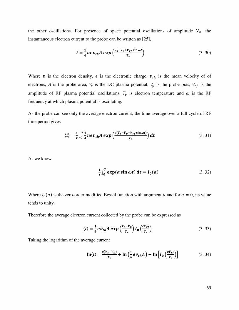
69
the other oscillations. For presence of space potential oscillations of amplitude Vrf, the
instantaneous electron current to the probe can be written as [25],
h = ]5 i Dò\ ò¯ò ¹Ü5Ù E (3. 30)
Where is the electron density, < is the electronic charge, IAJ is the mean velocity of of
electrons, is the probe area, óe is the DC plasma potential, ó) is the probe bias, óN is the
amplitude of RF plasma potential oscillations, î( is electron temperature and $ is the RF
frequency at which plasma potential is oscillating.
As the probe can see only the average electron current, the time average over a full cycle of RF
time period gives
h = Ù ]5 i D(ò\ ò¯ò ¹Ü5)Ù E b5Ù (3. 31)
As we know
Ù uà( ¹Ü5) b5Ù = |() (3. 32)
Where í;(") is the zero-order modified Bessel function with argument " and for " = 0, its value
tends to unity.
Therefore the average electron current collected by the probe can be expressed as
h = ]5 i Dò\ òÙ E | DòÙ E (3. 33)
Taking the logarithm of the average current
h = cò\ òdÙ + D ]5E + | DòÙ E (3. 34)
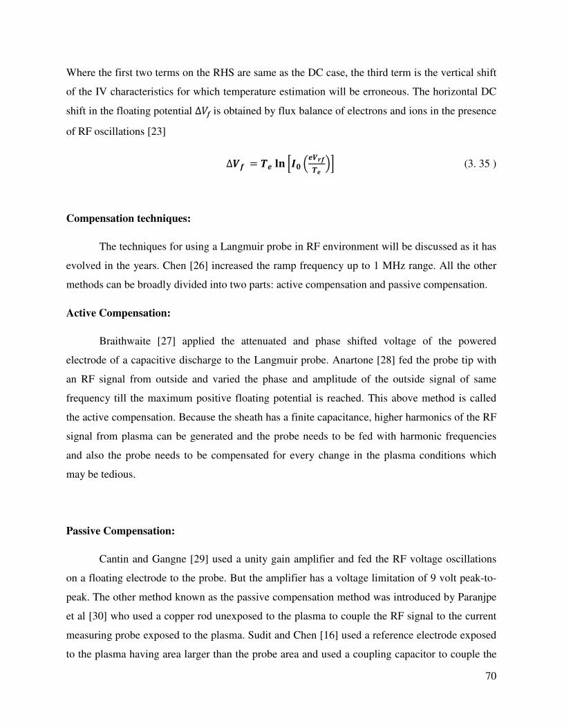
70
Where the first two terms on the RHS are same as the DC case, the third term is the vertical shift
of the IV characteristics for which temperature estimation will be erroneous. The horizontal DC
shift in the floating potential ∆ó is obtained by flux balance of electrons and ions in the presence
of RF oscillations [23]
∆ò = Ù | DòÙ E (3. 35 )
Compensation techniques:
The techniques for using a Langmuir probe in RF environment will be discussed as it has
evolved in the years. Chen [26] increased the ramp frequency up to 1 MHz range. All the other
methods can be broadly divided into two parts: active compensation and passive compensation.
Active Compensation:
Braithwaite [27] applied the attenuated and phase shifted voltage of the powered
electrode of a capacitive discharge to the Langmuir probe. Anartone [28] fed the probe tip with
an RF signal from outside and varied the phase and amplitude of the outside signal of same
frequency till the maximum positive floating potential is reached. This above method is called
the active compensation. Because the sheath has a finite capacitance, higher harmonics of the RF
signal from plasma can be generated and the probe needs to be fed with harmonic frequencies
and also the probe needs to be compensated for every change in the plasma conditions which
may be tedious.
Passive Compensation:
Cantin and Gangne [29] used a unity gain amplifier and fed the RF voltage oscillations
on a floating electrode to the probe. But the amplifier has a voltage limitation of 9 volt peak-to-
peak. The other method known as the passive compensation method was introduced by Paranjpe
et al [30] who used a copper rod unexposed to the plasma to couple the RF signal to the current
measuring probe exposed to the plasma. Sudit and Chen [16] used a reference electrode exposed
to the plasma having area larger than the probe area and used a coupling capacitor to couple the
71
RF fluctuations to the probe. They have used inductors as RF chokes which offer high
impedance to the RF signals at fundamental and higher harmonics. As the compensating
electrode is kept near to the probe, the compensation need not be changed every time.
Design:
Two single Langmuir probes are used out of which one is compensated and the other is
an uncompensated only for comparison. The picture of the probes is shown in Figure 3.15. The
uncompensated probe is same as described in the last section. The tungsten probe tips are
covered with thin ceramic pipe of 0.7 mm diameter and length 10 mm leaving an exposed tip of
3 mm length and 0.5 mm diameter for both the probes.
A winding of 30 turns of 125 micron tungsten filament is done over the ceramic pipe whose one
end is connected to one end of a ceramic capacitor of 10 nF capacitance which is kept inside the
hollow ceramic probe holder.
Figure 3.15 Picture of the RF compensated probe along with an
uncompensated probe.
The other end of the capacitor is connected to the probe tip from inside the probe shaft. The
probe length after the capacitor connection towards the measurement circuit is connected in
series with two self resonating inductors which act as chokes for RF f
and 27.12 MHz as shown in Figure 3.16.
The current signals from the plasma are carried by RG 174 coaxial cables which are connected to
Vacuum BNCs at the end of the flange connected to a vacuum feed
Figure 3.16 Schematic of the RF compensated probe along showing the
compensating winding, coupling capacitor and the self resonating RF chokes.
Figure 3.17 Comparison of IV characteristics of compensated and
uncompensated Langmuir probe.
The other end of the capacitor is connected to the probe tip from inside the probe shaft. The
probe length after the capacitor connection towards the measurement circuit is connected in
series with two self resonating inductors which act as chokes for RF frequencies of 13.56 MHz
and 27.12 MHz as shown in Figure 3.16.
The current signals from the plasma are carried by RG 174 coaxial cables which are connected to
Vacuum BNCs at the end of the flange connected to a vacuum feed-through. The IV
Schematic of the RF compensated probe along showing the
compensating winding, coupling capacitor and the self resonating RF chokes.
Comparison of IV characteristics of compensated and
uncompensated Langmuir probe.
72
The other end of the capacitor is connected to the probe tip from inside the probe shaft. The
probe length after the capacitor connection towards the measurement circuit is connected in
requencies of 13.56 MHz
The current signals from the plasma are carried by RG 174 coaxial cables which are connected to
through. The IV
Schematic of the RF compensated probe along showing the
compensating winding, coupling capacitor and the self resonating RF chokes.
Comparison of IV characteristics of compensated and
73
characteristics obtained at 250W RF power, 8x10⁻⁴ mbar and 100 G magnetic field are shown in
Figure 3.17 which shows a change in floating potential of ~ 15 V and the temperature obtained
are ~ 3.1 eV for uncompensated and ~ 2.9 eV for compensated probe.
3.5.4 Double Langmuir Probe
Though single Langmuir probes suffice as an electrostatic probe diagnostics in most of
the cases to determine density and temperature, they have certain limitations in specific plasmas
and plasma conditions. Single Langmuir probes always take the reference of the vessel wall
which in turn is in contact with the bulk plasma. This vacuum wall references are not available in
the case the plasma is produced in a dielectric chamber and also in electrodeless discharges.
Another limitation comes from the amount of probe current that is drawn to characterize the
plasma. In dilute, after glow and decaying plasmas where the probe current can be a significant
part of the discharge current, the probe may disturb the plasma. This is because of the larger
surface area of the vacuum vessel sheath. To get rid of these above stated problems Johnson and
Malter [31] have proposed a double Langmuir probe procedure in which another probe is placed
nearby to act as a reference and becomes the return path for the probe current. As this floating
probe draws a maximum current equal to the ion saturation current it can be used in dilute
plasmas.
Principle of operation:
The basic theory of operation can be understood from the electrical circuit diagram as
shown in Figure 3.18. When a bias is applied between the two probes, the probes collect current
but as the system is floating the currents to the probes are equal and opposite.
Let’s say, after a voltage V is applied to the probes, the two floating probes P1 and P2 attain
potentials of φ, and φ respectively.
Therefore
ò = Å − Å (3. 36 )

74
Let the plasma potential be φ÷ . The current in P1 of area A1 be I1 and in P2 of area A2 be I2 is
sum of the respective electron and ion currents.
| = − ] exp D Å Å Ù E + \3 (3. 37)
Rearranging,
− ] exp D Å Ù E = D | − \3E exp D Å Ù E (3. 38)
Similarly the current in P1 can be expressed in terms of plasma potential as
− ] exp D Å Ù E = D | − \3E exp D Å Ù E (3. 39)
Figure 3.18 Schematics of Double Langmuir probe measurement circuit.
Scope
P1
P2
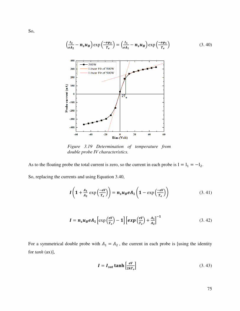
75
So,
D | − \3E exp D Å Ù E = D | − \3E exp D Å Ù E (3. 40)
As to the floating probe the total current is zero, so the current in each probe is I = I, = −I.
So, replacing the currents and using Equation 3.40,
| § + exp D òÙ E© = \3 § − exp D òÙ E© (3. 41)
| = \3 exp DòÙE − i DòÙE +
(3. 42)
For a symmetrical double probe with , = , the current in each probe is [using the identity
for tanh (ax)],
| = |\5 w òCÙ (3. 43)
Figure 3.19 Determination of temperature from
double probe IV characteristics.

76
Where the ion saturation current íeÔA = e<. Taking the slope near ó = 0 as shown in
Figure 3.19.
b|bòò = |\5ò = |\5 CÙ \6 D òCÙEò = |\5 × CÙ (3. 44)
ò = CÙ (3. 45)
tanh"o has slope of " for o = 0, we can calculate the temperature by just finding the slope of
the line passing through the origin of IV characteristics as shown in Figure 3.19. The double
probe characteristics measured at 4x10⁻³ mbar and 55 Gauss for powers 50-500 W are shown in
Figure 3.20.
Figure 3.20 Double Probe characteristics measured at z=22 cm for
different RF for powers 50-500 W with 4x10⁻³
mbar pressure and 55
Gauss magnetic field.

77
Design:
The double probe is made of two identical tungsten probe tips of 0.5 mm diameter and 3
mm exposed length. The bias is given by a floating power supply and the current flowing
through a series measuring resistance gives a voltage drop. This voltage is measured by an
oscilloscope through a unit optical isolation amplifier. The schematic of the measurement circuit
is shown in Figure 3.18.
3.5.5 Triple Langmuir Probe
Single Langmuir probe is widely used as a probe diagnostics for measurement of density
and temperature in plasmas. A metallic probe exposed to the plasma is biased w.r.t. the vessel
reference and the current collected is passed through a measuring resistance. The voltage drop
across the resistance is used to calculate the collected current. The probe current Vs bias voltage
gives the I-V characteristics of the probe. Temperature is deduced from the slope of the electron
collecting region of the probe characteristics. Density is obtained from the measured ion
saturation current and the deduced electron temperature. The first and foremost stringent
requirement is that the measurement needs a good reference of an appreciable area. Second, SLP
draws a large amount of current in the electron collection regime, which may be a part of the
discharge current in some plasma systems like afterglow plasma. Third, the amount of bias
applied even in case of a low temperature plasma can be very high when the plasma potential (or
floating potential) is of very high magnitude (either positive or negative). High bias voltages
often put a larger demand on the current measurement circuit. The above mentioned problems
are overcome by using a double Langmuir probe which does not need a reference and uses one
of the probe tips as a reference and also it draws a maximum current of ion saturation current.
The other problem involved in SLP which is not overcome by a DLP is the tedious data analysis,
which also cannot give the instantaneous values of temperature and density in case of time
varying plasma. If a high frequency bias is given, capacitive pick up as shown in Figure 3.11,
can generate noise currents comparable to ion saturation currents. This noise current produces a
voltage drop which may be comparable to the fluctuation (time varying parameters) signals.
To overcome all the previously mentioned shortcomings in SLP and DLP, a third probe is used
with a DLP. The third probe in addition to DLP constitutes the triple Langmuir probe (TLP). As
in DLP one of the probes collects ion current while the other collects the electron current, here in

78
TLP also one probe collects electron current equivalent of the ion saturation current collected by
a second probe with a third probe kept floating. The potential difference between the floating
reference probe and the electron current collecting probe is a measure of temperature if the later
collects an amount of electron current equal to the ion saturation current. The probe circuit
consisting of the reference probe and ion saturation collecting probe can accommodate a series
resistance across which the voltage can be measured to deduce ion saturation current in the
circuit. This ion saturation current along with the temperature obtained gives the density. As the
potential difference between floating probe and electron collecting probe is proportional to
electron temperature, instantaneous temperature fluctuations can be obtained using a TLP.
Working Principle:
In its simplest form [32-33] the triple-probe method employs three separate Langmuir
probes of identical shape and dimension placed a small distance apart and individually biased to
three different potentials (Figure 3.21) The probe potentials are less than the plasma potential so
that negatively biased sheaths exist around each probe. The spacing between probes must be
large enough to adequately shield them from one another. The current to each probe is the sum of
the ion saturation current and the electron current. By combining these conditions with the
current density equations, the triple-probe equations are derived. As all probe potentials are less
than the plasma potential, an ion sheath is formed around all the three probes. One of the
assumptions is that all the probes see the same plasma so that different characteristics do not
exist for different probes.
A triple Langmuir probe (TLP) [32] to get the instantaneous density and temperature is
used. If the potential of the three probes P1, P2 and P3 are respectively V1, V2 and V3 as shown in
Figure 3.22, we can define the following potentials and currents [33]
òb = ò − ò (3. 46)
òb = ò − ò (3. 47)
| = | + | (3. 48)

79
The Currents as shown in Figure 3.22 to all the three probes are í,, í and í. respectively and can
be written as −| = −|\5 uà D− òÙ E + |¯ (3. 49)
−| = −|\5 uà D− òÙ E + |¯ (3. 50)
−| = −|\5 uà D− òÙ E + |¯ (3. 51)
Figure 3.21 Schematics of the triple Langmuir probe circuit
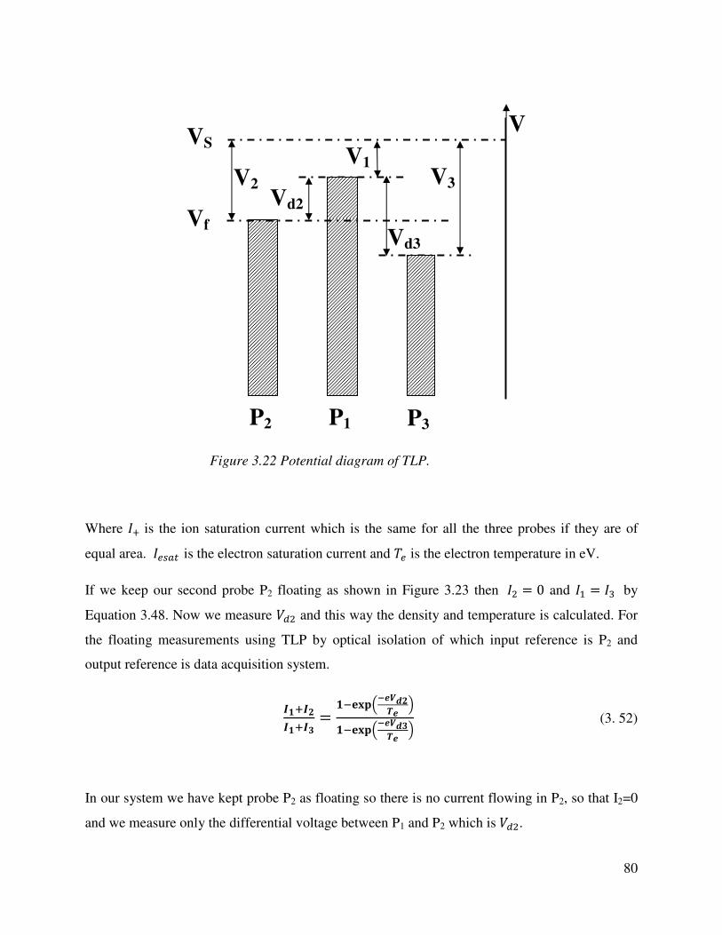
80
Where í is the ion saturation current which is the same for all the three probes if they are of
equal area. í(eÔA is the electron saturation current and î( is the electron temperature in eV.
If we keep our second probe P2 floating as shown in Figure 3.23 then í = 0 and í, = í. by
Equation 3.48. Now we measure ó! and this way the density and temperature is calculated. For
the floating measurements using TLP by optical isolation of which input reference is P2 and
output reference is data acquisition system.
|¯||¯| = uàDªòbÙ E uàDªòbÙ E (3. 52)
In our system we have kept probe P2 as floating so there is no current flowing in P2, so that I2=0
and we measure only the differential voltage between P1 and P2 which is ó!.
V2 Vd2
V
V1
Vd3
V3
Vf
VS
P2 P1 P3
Figure 3.22 Potential diagram of TLP.

81
| = | as | = (3. 53)
So the new set of relations for deducing temperature and density will be
= uàDªòbÙ E uàDªòbÙ E (3. 54)
|¯ = | ¯uàDªòbÙ E uàDªòbÙ E (3. 55)
In the case, <ó!. ≫ 2î(, the expression for temperature is î( = 1.44ó!. This value of
temperature when used in ion saturation current expression gives density. We have given a
Figure 3.23 Modified circuit of TLP with optical isolation for
instantaneous display of ion saturation current and temperature.

82
floating bias of 30 V which is more than twice of every temperature range in our experiment. For
ion saturation current, í ~í,for <ó!. ≫ 2î(.
Design:
Three probes of 0.5 mm diameter and 3 mm length are used as probe tips. All the
connections are made with RG 174 coaxial cables. Two optical isolation amplifiers are used to
isolate the measurement reference (P1) and the acquisition circuit reference (scope) for ion
saturation and floating voltage measurements. These amplifiers have bandwidth of 250 kHz.
Low pass filters (mini-circuits make low pass filters) have been used to filter out RF interference
if any.
3.5.6 Emissive Probe
Plasma potential and its fluctuations are important parameters that can characterize
electric fields and their fluctuations inside plasma. Using a cold probe we have seen in section
3.5.1that, plasma potential can be estimated from the floating potential when you have the
information of the electron temperature. But the estimation of electron temperature is often
tedious. Also in the presence of electron beams or drifted electrons floating potential cannot give
correct values of plasma potential. So, hot probes are often used to find the plasma potential. The
hot or emissive probe works on the principle that the emitted electrons compensate for the ion
sheath for probe biases below the plasma potential, so that the floating potential of the hot probe
is always near the plasma potential (no ion sheath) for high enough emission irrespective of
presence of fast or drifted electrons.
Working Principle:
The current in I-V characteristics has components from the collected current and emitted
current. Neglecting the space charge effects, the emitted current can be expressed as [34]:
|(ò) = "| i#−cò − òd Ù$⁄ %cò − òd, ò ≥ ò | , ò ≤ ò ( (3. 56)

83
Where V) is the probe bias, V÷ is the plasma potential, T* is the wire temperature, fcV) − V÷d
accounts for orbital angular momentum of emitted electrons (depends on the wire radius and the
dimensions of the sheath separating the wire from the virtual anode formed by the plasma). Here
Iú,; is the temperature limited emission current given by the Richardson-Dushman equation
expressed as
| = Ù$ i DÅ$Ù$ E, (3. 57)
Where A is the Richardson’s constant, φ* is the work function of the wire material, S is the
surface area of the wire. In case of emission of the filament inside the plasma, the emitted current
is constant for bias less than plasma potential because the emitted electrons do not see any
retarding potential (neglecting space charge effects). So the emitted electrons behave like
collection of ions by the probe, so that the overall current is replenished by these emitted
electrons below the plasma potential. When a bias above plasma potential is applied, the
electrons feel a retarding force for the plasma acts like a cathode and the emission current
decreases rapidly. As the emitted electrons are in equilibrium with a temperature of the order of
the probe temperature which is of the order of few tenth of eV, the transition region of constant
emission to almost no emission is very sharp.
The collected current is the current collected by a cold Langmuir probe and can be expressed as
|(ò) = "| i#cò − òd Ù⁄ % , ò ≤ ò,| Õcò − òd , ò ≥ ò. ( (3. 58)
Where, Iú; is the electron saturation current, Tú is the electron temperature in eV and f ′cV) −Vp accounts for the orbital angular momentum of collected electrons. When the bias is very

negative w.r.t. plasma potential, the probe collects ion saturation current and then when the bias
is increased the probe starts collecting electrons and all the electrons are collected near plasma
potential and the collected current ideally becomes consta
Methods of Emissive Probe:
Floating potential method:
The floating potential of a sufficiently heated emissive probe is close to the local plasma
potential, and this is the most widely used method for plasma potential determination and the
most convenient method [36]. When a probe emits thermionically, the sh
front of the emissive probe decrease for the emitted electron currents compensate for the ion
currents. When the probe is strongly heated such that there is no sheath in front of the probe, the
floating potential of the probe approac
the saturated floating potential of the probe is close to the plasma potential. When measuring
floating potential we are using a high series resistance which will have a load line almost parallel
Figure 3.24 IV characteristics of an emissive probe showing the
bias dependence contributions from emission current and
collection current [35]
negative w.r.t. plasma potential, the probe collects ion saturation current and then when the bias
is increased the probe starts collecting electrons and all the electrons are collected near plasma
potential and the collected current ideally becomes constant near or above the plasma potential.
The floating potential of a sufficiently heated emissive probe is close to the local plasma
potential, and this is the most widely used method for plasma potential determination and the
most convenient method [36]. When a probe emits thermionically, the sheath potential drop in
front of the emissive probe decrease for the emitted electron currents compensate for the ion
currents. When the probe is strongly heated such that there is no sheath in front of the probe, the
floating potential of the probe approaches the plasma potential. As can be seen from the figure
the saturated floating potential of the probe is close to the plasma potential. When measuring
floating potential we are using a high series resistance which will have a load line almost parallel
IV characteristics of an emissive probe showing the
bias dependence contributions from emission current and
[35].
84
negative w.r.t. plasma potential, the probe collects ion saturation current and then when the bias
is increased the probe starts collecting electrons and all the electrons are collected near plasma
nt near or above the plasma potential.
The floating potential of a sufficiently heated emissive probe is close to the local plasma
potential, and this is the most widely used method for plasma potential determination and the
eath potential drop in
front of the emissive probe decrease for the emitted electron currents compensate for the ion
currents. When the probe is strongly heated such that there is no sheath in front of the probe, the
hes the plasma potential. As can be seen from the figure
the saturated floating potential of the probe is close to the plasma potential. When measuring
floating potential we are using a high series resistance which will have a load line almost parallel
IV characteristics of an emissive probe showing the
bias dependence contributions from emission current and

85
to the voltage axis of figure 3.25. This load line intercepts the prove IV characteristics of each
curve near the floating potential i.e. current to the probe is almost zero. As the heating current
increases the incremental shift in floating potential decreases and saturates for high enough
heating current. This saturation floating potential corresponds to the plasma potential.
Inflection point method:
For an emissive probe when the bias is less than the plasma potential, the current in the
probe circuit is because of both emission and collection currents. When the bias is near or more
than plasma potential, the current to the probe is changes as the total current is now only the
collection current with no emitted electrons are accepted by the plasma. So the differentiated IV
characteristic of an emissive probe shows a peak at the plasma potential [35]. This is illustrated
in Figure 3.26.
Figure 3.25 Plasma potential determination by floating potential method
where an emitting probe’s floating potential approaches the local plasma
potential for strong emission [37].

Separation point method:
The potential at which characteristics of a cold probe and strongly emitting probe start to
deviate is known as the plasma potential [38
probe is strongly emitting, the electron saturation current of the cold probe must be equal to that
of the ion saturation current of a strongly emitting probe. But as in many cases, either because of
RF field effects or geometry effects we do not get the electro
comings of space charge effects as one would work in a strong emission conditions.
Figure 3.26 Plasma potential determination by inflection point method
where the differentiated IV characteristic of a partially emitting hot
probe has an inflection point
Figure 3.27 Plasma potential determination by separation point method where
the IV characteristic
The potential at which characteristics of a cold probe and strongly emitting probe start to
deviate is known as the plasma potential [38-39] as shown in Figure 3.27. But to ensure that the
is strongly emitting, the electron saturation current of the cold probe must be equal to that
of the ion saturation current of a strongly emitting probe. But as in many cases, either because of
RF field effects or geometry effects we do not get the electron saturation, this method has short
comings of space charge effects as one would work in a strong emission conditions.
Plasma potential determination by inflection point method,
where the differentiated IV characteristic of a partially emitting hot
probe has an inflection point near the plasma potential [35].
Plasma potential determination by separation point method where
the IV characteristics of cold and hot probes separate from each other.
86
The potential at which characteristics of a cold probe and strongly emitting probe start to
39] as shown in Figure 3.27. But to ensure that the
is strongly emitting, the electron saturation current of the cold probe must be equal to that
of the ion saturation current of a strongly emitting probe. But as in many cases, either because of
n saturation, this method has short
comings of space charge effects as one would work in a strong emission conditions.
,
where the differentiated IV characteristic of a partially emitting hot
Plasma potential determination by separation point method where
e from each other.
87
Effect of space charge limited emission:
When the emission current is less such that the floating potential of the emissive probe is
less than the plasma potential, an ion sheath is formed around the emissive probe. The emitted
electrons thus see a monotonic potential and get accelerated to the plasma. But when the
emission current is increased a condition comes when there is no sheath around the probe.
Further increasing the emission, the emitted electrons make a virtual cathode which can send
back all or part of the emitted electrons back to the probe [40]. This is called the space charge
limited emission and observed for high emission currents. This is a drawback of floating
potential method of plasma potential determination using emissive probe. One can always check
for the space charge effect by increasing the emission current to a level where the floating
potential value saturates but does not decrease upon increasing heating current. That’s why in
floating potential method very high heating currents are not used. The inflection point method
has overcome this problem as the plasma potential can be determined for low heating currents
without strong emission.
Ye and Takamura [40] have done the analytical calculations including the space charge effect
and found a relation between the floating potential and plasma potential as
ò = ò + À DÙ E (3. 59)
, where à has the value of -0.95, -0.99 and -1.01 respectively for hydrogen, helium and argon.
Effect of RF potential fluctuations:
When the plasma potential oscillates with a frequency such that the emissive probe
cannot follow the potential fluctuations, then the average current collected by an emissive probe
has two slopes. In case of inflection point method when the emission current is low, !.!/ has two
peaks for potential fluctuations more than electron temperature with the two peaks corresponding
to the minimum and maximum value of the RF amplitude [41-42]. The value of the plasma
potential then is given by the average value of these two peaks. In the case of floating potential
method however with strong emission, the value of plasma potential obtained so remains
unaffected.

88
Effect of Magnetic field:
When the probe radius is larger than the electron larmour radius, the electrons that leave
the surface of the filament can come back to the filament so that a space charge region will be
formed. When the filament arch surface is perpendicular to the magnetic field a JXB force acts
on the filament and there is a chance that it may get deformed or broken [36]. But as we are
using a thin filament of 0.125 mm for which the current requirement for strong emission is less
all the two problems discussed above can be neglected for the magnetic fields used in this thesis.
Measurement accuracy and errors:
The plasma potential obtained using an emissive probe is accurate up to potential
equivalent of probe temperature î0 <⁄ . In floating potential method the probe potential is
measured with a high series impedance when the emission is strong for which a finite current
passes through the filament. Therefore a finite voltage 2∆ó drops across the filament. This
voltage has to be subtracted to find the real floating potential. But for that it is necessary to know
out of two legs to which the measuring circuit is connected. Marvlag et al [43] have shown that
when emission current is equal to the electron saturation current (or for strong emission)
ò\ = ò ± ∆ò (3. 60)
Where the sign depends on which leg is connected to the measurement circuit.
Design:
The loop of the emissive probe is made of tungsten filament of 0.125 mm. The length of
the filament is 10 mm and diameter of the loop is ~ 3mm. The tungsten loop is inserted inside a
twin bore ceramic tube of 2.5 mm outer diameter (Figure 3.28). The electrical connections are
made by spiraling the tungsten filament’s extended length over small copper strands. Tungsten
wires 0.5 mm diameter and 6 mm length are used to fill the gaps inside which also act to decrease
the filament heat load.
The copper strands used to wrap the filament are then soldered with the current carrying
copper wires and the wires are taken outside using vacuum BNCs. The heating current required
for 0.125 mm diameter tungsten wire is in between 2.5-3 Ampere which is supplied by an Aplab
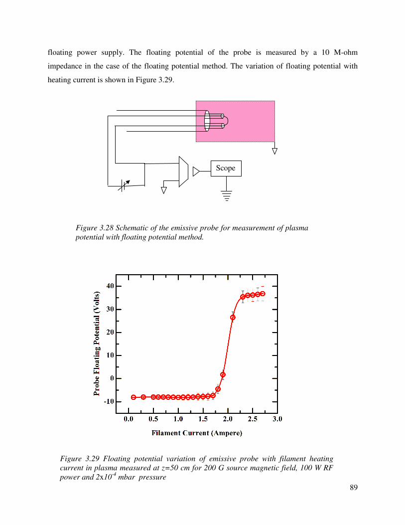
89
floating power supply. The floating potential of the probe is measured by a 10 M-ohm
impedance in the case of the floating potential method. The variation of floating potential with
heating current is shown in Figure 3.29.
Figure 3.28 Schematic of the emissive probe for measurement of plasma
potential with floating potential method.
Figure 3.29 Floating potential variation of emissive probe with filament heating
current in plasma measured at z=50 cm for 200 G source magnetic field, 100 W RF
power and 2x10⁻⁴
mbar pressure
Scope

90
3.5.7 B-dot Probe
B-dot probes are widely used to measure magnetic field fluctuations in plasmas [44-51].
Multiple loop B-dot probes are often used to increase the output signal strength. However, in
case of RF plasma, significant oscillating potential differences [47] can be present between a
magnetic probe and plasma (and antenna). A magnetic probe can couple capacitively to these
oscillating potentials in the plasma or antenna. This pick up signal depends on the potential
amplitude, the capacitance between the probe and plasma and the terminating resistance. Often a
50 Ohm terminating resistance is used to reduce the electrostatic pick up. But sometimes this is
not enough at least when the wave field amplitudes are small. To get rid of this capacitive pick
up some techniques like hybrid combiners or baluns are often used. Another method, that has an
inherent capacitive pick up rejection can be used is a single loop B-dot probe made of a co-axial
cable as shown in Figure 3.31. The use of this kind of probe is limited to higher frequencies
though.
Single loop B-dot probes are used to characterize the mode structure of helicon waves [4] and to
measure the parallel wave length of the helicon waves. The magnitudes of perpendicular wave
magnetic field components are measured to characterize and confirm m=+1 helicon modes. Two
probes are used to measure helicon wave axial wavelength. This is done by taking one probe as
reference probe and its phase as the reference for phase measurement. The other probe is
translated axially and the phase variation along axis is noted. The slope of the phase variation is
used to estimate the wavelength or the wave number of the helicon wave.
Working principle:
Whenever a time varying magnetic flux cuts a surface of a conducting loop, a voltage is
induce in the ends of the loop. As per faraday’s law
Ì × 2778 = − 4377845 (3. 61)
Integrating over the surface area of the coil and taking sinusoidal variations of fields,
cÌ × 2778d. br = − 3778. br (3. 62)
Where dA is the differential area and ns is vector normal to the plane of the coil. Using Stoke’s
theorem

Where A is the total area of the coil and
the loop. This gives the induced voltage in the loop which can be expressed as
For we are interested only fluctuations in the 13.56
probe, which reduces the parasitic capacitance and the inductance and gives enough signal to
noise ratio. The area of the coil is 10
RG174 coaxial cable of 1.8 mm
centre conductor is connected to the nearest shielding of the loop as shown in Figure 3.30.
Electrostatic pick up is reduced in this design. The probes are checked for electrostatic pick u
noise by rotating the probe 180 degree. The results for measurement of amplitude of helicon
wave axial component Bz for 300W RF power, 2x10
probe inserted from a radial port at z=22 cm is shown in Figure 3.31. T
rotated by 180 degree shows a phase variation of 180 degree and also the signal amplitude is
same as 0 degree as expected for a voltage output induced in the probe due to magnetic field
oscillations only. This confirms the inherent capac
Figure 3.30 Picture of the single loop B
coaxial cable.
12778. b277778 = −3778. r
Where A is the total area of the coil and dl is a differential line segment along the perimeter of
voltage in the loop which can be expressed as
ò2GG = 3 ·¸¹
For we are interested only fluctuations in the 13.56 MHz, we have used a single loop B
probe, which reduces the parasitic capacitance and the inductance and gives enough signal to
noise ratio. The area of the coil is 10 mm2 and the radius of the loop is 3 mm. It is made up of a
diameter. At one end the cable is looped and after the loop the
centre conductor is connected to the nearest shielding of the loop as shown in Figure 3.30.
Electrostatic pick up is reduced in this design. The probes are checked for electrostatic pick u
noise by rotating the probe 180 degree. The results for measurement of amplitude of helicon
for 300W RF power, 2x10⁻³ mbar and 30 G magnetic field using this
probe inserted from a radial port at z=22 cm is shown in Figure 3.31. The probe axis when
rotated by 180 degree shows a phase variation of 180 degree and also the signal amplitude is
same as 0 degree as expected for a voltage output induced in the probe due to magnetic field
oscillations only. This confirms the inherent capacitive pick up rejection of this single loop
Picture of the single loop B-dot probe made of a
91
(3. 63)
is a differential line segment along the perimeter of
(3. 64)
, we have used a single loop B-dot
probe, which reduces the parasitic capacitance and the inductance and gives enough signal to
. It is made up of a
diameter. At one end the cable is looped and after the loop the
centre conductor is connected to the nearest shielding of the loop as shown in Figure 3.30.
Electrostatic pick up is reduced in this design. The probes are checked for electrostatic pick up
noise by rotating the probe 180 degree. The results for measurement of amplitude of helicon
mbar and 30 G magnetic field using this
he probe axis when
rotated by 180 degree shows a phase variation of 180 degree and also the signal amplitude is
same as 0 degree as expected for a voltage output induced in the probe due to magnetic field
itive pick up rejection of this single loop

92
coaxial B-dot probe. The shielding helps in two ways. One it forms a part of the loop and at the
same time acts as shield for electrostatic signals inside the plasma, which are because of the high
RF voltage fluctuations of the plasma potential. Also the low frequency signals in kHz range of
frequencies cannot induce enough voltage more than the noise level of the probe to get detected.
3.5.8 Antenna-Plasma Load Measurements
A rogowski or RF current probe (CT) is used to measure the antenna RF current flowing
in the antenna circuit. The antenna current is a measure of antenna-plasma resistance and RF
power transfer efficiency in any RF plasma system when the reflected power is negligible when
compared to the forward power. A Pearson 410 [ref] rogowski is inserted around the antenna
transmission line leg just after the match box. This rogowski has the high frequency 3 dB point at
20 MHz, a peak current value of 5 kA and peak RMS current value of 50 A. The output of this
CT has a calibration factor or sensitivity of 0.1 V/A. The CT has a BNC output which is
Figure 3.31 The graphs showing the inherent electrostatic pick up rejection
by use of a single loop b-dot probe. The probe output for 0 deg (red), 180 deg
(black) and 360 deg (blue) showing the capacitive pick up is negligible.

93
connected to a 50 Ohm BNC and subsequently the output is monitored with a digital
oscilloscope of 1 M-ohm input impedance which necessitates a termination of 50 Ohm before
connecting to the oscilloscope. Using the above mentioned calibration factor the output voltage
is noted and later converted to current values. Having the knowledge of the values of forward
power Pfor, reflected power Pref, the RMS current value the total antenna resistance can be written
as for reflections <1% as [7]
5G5 = G | (3. 65)
Here ¡A3A is the sum of the antenna vacuum resistance RA and the antenna-plasma resistance RP.
The antenna vacuum resistance is calculated by powering the antenna without plasma and noting
down the RMS value of antenna current. This vacuum current is used to drive the antenna
resistance which is actually the sum of skin resistances (of antenna, transmission line, and match
box inductors), contact resistances of all the frictional electrical connections and eddy current
losses. Once RA is known, the plasma resistance RP is calculated by subtracting the value of RA
from Rtot which is obtained in the presence of the plasma. RP is the sum of all the plasma
processes leading to heating, ionization and maintaining the plasma thus is a sum of all the
capacitive, inductive and wave coupling depending upon the discharge conditions. The power
transfer efficiency 4 is the ratio of absorbed power Pabs and the total supplied RF power Ptot and
is expressed as follows
5 = \5G5 = ¯ (3. 66)
The efficiency and plasma resistance both increase when the discharge transitions from a
capacitive to inductive to Helicon wave mode.
3.6 Summary of Chapter 3
A linear helicon plasma device with controllable magnetic field gradient is designed and
developed. Vacuum levels of 1x10⁻⁶ mbar are achieved. RF matching is done using an L-type
matching network with less than 1 % reflection. Various probes with their electronics are
designed, developed and tested in plasma with low level of noise. Working principles of all the
probes are discussed.
94
References
[1] S. J. Sackett, EFFI Code (Lawrence Livermore National Laboratory, California, (1978).
[2] Porte, L., S. M. Yun, D. Arnush, and F. F. Chen. "Superiority of half-wavelength helicon antennae." Plasma Sources Science and Technology 12, no. 2 (2003): 287.
[3] Chen, Francis F. "Capacitor tuning circuits for inductive loads." UCLA Report (1992).
[4] Light, Max, and Francis F. Chen. "Helicon wave excitation with helical antennas." Physics of
Plasmas 2 (1995): 1084.
[5] Kamenski, I. V., and G. G. Borg. "An evaluation of different antenna designs for helicon wave excitation in a cylindrical plasma source." Physics of Plasmas 3 (1996): 4396.
[6] Boswell, Rod W., and Francis F. Chen. "Helicons-the early years." Plasma Science, IEEE
Transactions on 25, no. 6 (1997): 1229-1244.
[7] Lafleur, T., C. Charles, and R. W. Boswell. "Characterization of a helicon plasma source in low diverging magnetic fields." Journal of Physics D: Applied Physics 44, no. 5 (2011): 055202.
[8] Mott-Smith, H. M., & Langmuir, I. (1926). The theory of collectors in gaseous discharges. Physical Review, 28(4), 727.
[9] F. F. Chen, in Plasma Diagnostic Techniques, ed. by R. H. Huddlestone and S. L. Leonard (Academic Press, New York, 1965)
[10] L. Schott, in Plasma Diagnostics, ed. by W. Lochte-Holtgreven (John Wiley, New York, 1968)
[11] I. H. Hutchinson, Principles of Plasma Diagnostics, (Cambridge University Press, 1987)
[12] N. Hershkowitz, How Langmuir Probes Work, in Plasma Diagnostics, Discharge Parameters and Chemistry, ed. by O.Aucillo and. D.L. Flamm (Academic Press, 1989)
[13] Demidov, V. I., Ratynskaia, S. V., & Rypdal, K. (2002). Electric probes for plasmas: The link between theory and instrument. Review of scientific instruments, 73(10), 3409-3439.
[14] N. A. Krall and A. W. Trivelpiece, Principles of Plasma Physics, (San Francisco Press, 1986)
[15] J. C. Sprott, Electrostatic Probe Techniques, PLP 88, University of Wisconsin, Madison (1966)
[16] Sudit, I. D., & Chen, F. F. (1994). RF compensated probes for high-density discharges. Plasma Sources Science and Technology, 3(2), 162.
[17] Sheridan, T. E. "How big is a small Langmuir probe?." Physics of Plasmas 7 (2000): 3084.
[18] Sheridan, T. E. "The plasma sheath around large discs and ion collection by planar Langmuir probes." Journal of Physics D: Applied Physics 43, no. 10 (2010): 105204.
95
[19] Lee, Dongsoo, and Noah Hershkowitz. "Ion collection by planar Langmuir probes: Sheridan’s model and its verification." Physics of plasmas 14 (2007): 033507.
[20] Demidov, V. I., Svetlana V. Ratynskaia, and K. Rypdal. "Electric probes for plasmas: The link between theory and instrument." Review of scientific instruments 73, no. 10 (2002): 3409-3439.
[21] Hutchinson, Ian H. "A fluid theory of ion collection by probes in strong magnetic fields with plasma flow." Physics of Fluids 30 (1987): 3777.
[22] Butler, H. S., and G. S. Kino. "Plasma Sheath Formation by Radio‐Frequency Fields." Physics of Fluids 6 (1963): 1346.
[23] Chabert, Pascal, Nicholas Braithwaite, and Nicholas St J. Braithwaite. Physics of Radio-
Frequency Plasmas. Cambridge University Press, 2011.
[24] Aanesland, A., Charles, C., Boswell, R. W., & Fredriksen, Å, Sputtering effects in a helicon plasma with an additional immersed antenna. Plasma Sources Science and Technology, 12, 85 (2003).
[25] Garscadden, Alan, and Karl George Emeléus. "Notes on the effect of noise on Langmuir probe characteristics." Proceedings of the Physical Society 79, no. 3 (1962): 535.
[26] Chen, Francis F. "Double‐Probe Method for Unstable Plasmas." Review of Scientific
Instruments 35, no. 9 (1964): 1208-1212.
[27] Braithwaite, N. St J., N. M. P. Benjamin, and J. E. Allen. "An electrostatic probe technique for RF plasma." Journal of Physics E: Scientific Instruments20, no. 8 (1987): 1046.
[28] Annaratone, B. M., and N. St J. Braithwaite. "A comparison of a passive (filtered) and an active (driven) probe for RF plasma diagnostics." Measurement Science and Technology 2, no. 8 (1991): 795.
[29] Cantin, A., and R. R. J. Gagne. "Pressure dependence of electron temperature using rf‐floated electrostatic probes in rf plasmas." Applied Physics Letters 30, no. 7 (1977): 316-319.
[30] Paranjpe, Ajit P., James P. McVittie, and Sidney A. Self. "A tuned Langmuir probe for measurements in rf glow discharges." Journal of Applied Physics 67, no. 11 (1990): 6718-6727.
[31] Johnson, E. O., & Malter, L. A floating double probe method for measurements in gas discharges. Physical Review, 80, 58 (1950).
[32] Chen, S. L., & Sekiguchi, T. (1965). Instantaneous Direct‐Display System of Plasma Parameters by Means of Triple Probe. Journal of Applied Physics, 36(8), 2363-2375.
[33] Ji, H., H. Toyama, K. Yamagishi, S. Shinohara, A. Fujisawa, and K. Miyamoto. "Probe measurements in the REPUTE‐1 reversed field pinch." Review of scientific instruments 62, no. 10 (1991): 2326-2337.

96
[34] Langmuir, Irving, and Karl T. Compton. "Electrical discharges in gases part II. Fundamental phenomena in electrical discharges." Reviews of modern physics3, no. 2 (1931): 191.
[35] Smith, J. R., Noah Hershkowitz, and P. Coakley. "Inflection‐point method of interpreting emissive probe characteristics." Review of Scientific Instruments50, no. 2 (1979): 210-218.
[36] Kemp, Robert F., and J. M. Sellen. "Plasma potential measurements by electron emissive probes." Review of Scientific Instruments 37, no. 4 (1966): 455-461.
[37] Makowski, M. A., and G. A. Emmert. "New method to measure plasma potential with emissive probes." Review of Scientific Instruments 54, no. 7 (1983): 830-836.
[38] Chen F. F. Plasma Diagnostic Techniques ed. R H Huddlestone and S L Leonard (NewYork; Academic Press, 1965) p. 113.
[39] C R Hoffmann and D J Lees “A differential method of measuring plasma potential” Plasma
Physics 13 pg. 689 (1971)
[40] Ye, M. Y., and S. Takamura. "Effect of space-charge limited emission on measurements of plasma potential using emissive probes." Physics of Plasmas7 (2000): 3457.
[41] Lho, T., N. Hershkowitz, and G. H. Kim. "Effect of harmonic rf fields on the emissive probe characteristics." Review of Scientific Instruments 71, no. 2 (2000): 403-405.
[42] Wang, E. Y., N. Hershkowitz, T. Intrator, and C. Forest. "Techniques for using emitting probes for potential measurement in rf plasmas." Review of scientific instruments 57, no. 10 (1986): 2425-2431.
[43] Mravlag, E., and P. Krumm. "Space potential measurements with a continuously emitting probe." Review of Scientific Instruments 61, no. 8 (1990): 2164-2170.
[44] R. H. Lovberg, in Plasma Diagnostic Techniques, edited by Richard H. Huddlestone and Stanley L. Leonard (Academic, New York, 1965), Chap. 3.
[45] W. Bötticher, in Plasma Diagnostics, edited by W. Lochte-Holtgreven (North Holland, Amsterdam, 1968), Chap. 10.
[46] Awasthi, L. M., S. K. Mattoo, R. Jha, R. Singh, and P. K. Kaw. "Study of electromagnetic fluctuations in high beta plasma of a large linear device."Physics of Plasmas 17 (2010): 042109.
[47] Reilly, Michael P., William Lewis, and George H. Miley. "Magnetic field probes for use in radio frequency plasma." Review of Scientific Instruments 80, no. 5 (2009): 053508-053508.
[48] Everson, E. T., P. Pribyl, C. G. Constantin, A. Zylstra, D. Schaeffer, N. L. Kugland, and C. Niemann. "Design, construction, and calibration of a three-axis, high-frequency magnetic probe (B-dot probe) as a diagnostic for exploding plasmas." Review of Scientific Instruments 80 (2009): 113505.
[49] Franck, Christian M., Olaf Grulke, and Thomas Klinger. "Magnetic fluctuation probe design and capacitive pickup rejection." Review of scientific instruments73, no. 11 (2002): 3768-3771.

97
[50] Eom, G. S., G. C. Kwon, I. D. Bae, G. Cho, and W. Choe. "Heterodyne wave number measurement using a double B-dot probe." Review of Scientific Instruments 72, no. 1 (2001): 410-412.
[51] Loewenhardt, P. K., B. D. Blackwell, and Beichao Zhang. "A simple miniature magnetic probe with inherent electrostatic rejection." Review of scientific instruments 64, no. 11 (1993): 3334-3335.
[52] http://www.pearsonelectronics.com/pdf/410.pdf
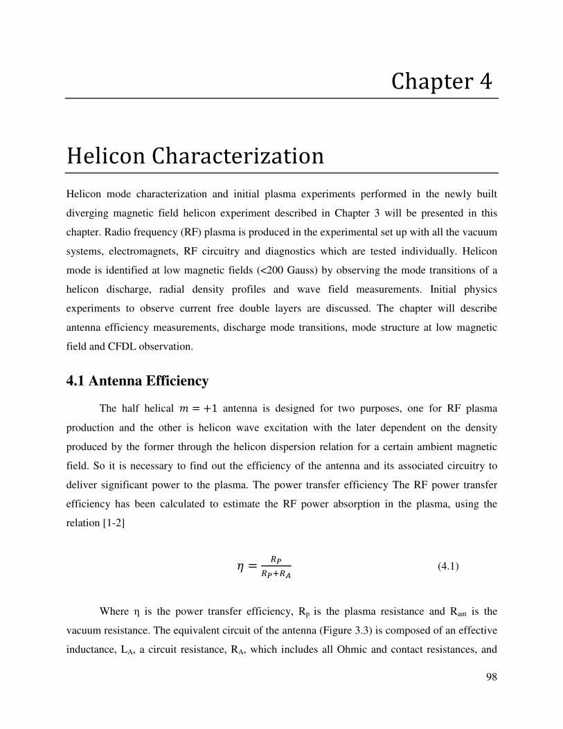
98
Chapter 4
Helicon Characterization
Helicon mode characterization and initial plasma experiments performed in the newly built
diverging magnetic field helicon experiment described in Chapter 3 will be presented in this
chapter. Radio frequency (RF) plasma is produced in the experimental set up with all the vacuum
systems, electromagnets, RF circuitry and diagnostics which are tested individually. Helicon
mode is identified at low magnetic fields (<200 Gauss) by observing the mode transitions of a
helicon discharge, radial density profiles and wave field measurements. Initial physics
experiments to observe current free double layers are discussed. The chapter will describe
antenna efficiency measurements, discharge mode transitions, mode structure at low magnetic
field and CFDL observation.
4.1 Antenna Efficiency
The half helical = +1 antenna is designed for two purposes, one for RF plasma
production and the other is helicon wave excitation with the later dependent on the density
produced by the former through the helicon dispersion relation for a certain ambient magnetic
field. So it is necessary to find out the efficiency of the antenna and its associated circuitry to
deliver significant power to the plasma. The power transfer efficiency The RF power transfer
efficiency has been calculated to estimate the RF power absorption in the plasma, using the
relation [1-2]
4 = 66¯7 (4.1)
Where η is the power transfer efficiency, Rp is the plasma resistance and Rant is the
vacuum resistance. The equivalent circuit of the antenna (Figure 3.3) is composed of an effective
inductance, LA, a circuit resistance, RA, which includes all Ohmic and contact resistances, and

99
any eddy current losses relevant to the antenna, transmission line and the matching network. The
plasma resistance, Rp includes all power losses attributed to the plasma, including power losses
due to capacitive, inductive and wave coupling. Since the total reactance of the combination of
antenna and plasma is matched under every measurement condition and the observed reflected
power is < 1%, total input power from the RF generator must be dissipated in the combined
antenna-plasma system. The total current in the antenna is related to the total effective antenna
loading resistance, Reff = RA + Rp, and the net power flow to the antenna is given by [2]
8 − = íNÎe ¡( (4.2)
Where 8 and are the forward and reflected powers respectively and Irms = Irf/√2 with Irf is the
amplitude of the sinusoidally varying current measured by a RF current probe coaxially held
around the reference leg of the transmission line. The external circuit resistance RA is estimated
by measuring the antenna current in the absence of plasma.
Figure 4.1 Variation of antenna RMS current and antenna
resistance with RF power in vacuum at × mbar.
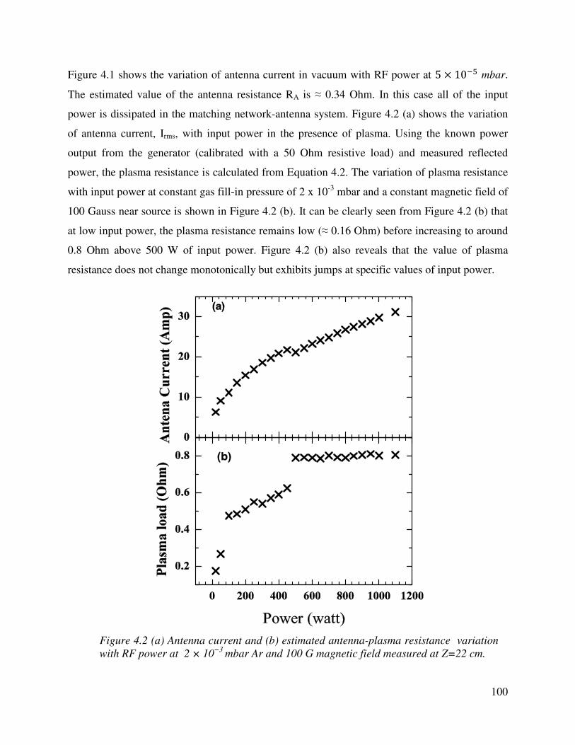
100
Figure 4.1 shows the variation of antenna current in vacuum with RF power at 5 × 10 9 mbar.
The estimated value of the antenna resistance RA is ≈ 0.34 Ohm. In this case all of the input
power is dissipated in the matching network-antenna system. Figure 4.2 (a) shows the variation
of antenna current, Irms, with input power in the presence of plasma. Using the known power
output from the generator (calibrated with a 50 Ohm resistive load) and measured reflected
power, the plasma resistance is calculated from Equation 4.2. The variation of plasma resistance
with input power at constant gas fill-in pressure of 2 x 10⁻³ mbar and a constant magnetic field of
100 Gauss near source is shown in Figure 4.2 (b). It can be clearly seen from Figure 4.2 (b) that
at low input power, the plasma resistance remains low (≈ 0.16 Ohm) before increasing to around
0.8 Ohm above 500 W of input power. Figure 4.2 (b) also reveals that the value of plasma
resistance does not change monotonically but exhibits jumps at specific values of input power.
Figure 4.2 (a) Antenna current and (b) estimated antenna-plasma resistance variation
with RF power at 2 × 10⁻³
mbar Ar and 100 G magnetic field measured at Z=22 cm.

101
These jumps in plasma resistance at around 40 W and 450 W of input power are indicative of
transitions from capacitive to inductive mode and inductive to helicon mode respectively, which
will be discussed elaborately in the next section. After determining the plasma resistance, the
power transfer efficiency η has been calculated. For low input powers (< 50 W), the power
transfer efficiency is less than 30% and it rises up to 75% for input power of > 1200 W which is
typical for a helicon discharge [1].
4.2 Discharge mode transitions
As discussed in Chapter 2, the discharge mode transitions are observed in all RF
discharges. In helicon literature [3] the modes are named E, H or W depending on the dominant
electric field responsible for maintain the discharge is of capacitive, inductive or wave origin
respectively. EHW mode transitions in helicon discharges are observed by changing source
parameters either of RF power [1, 3-4] and ambient magnetic field [5]. These transitions are
observed by monitoring the density [3-6], Q-factor of matching circuit [6], plasma potential [7]
or antenna plasma resistance [8]. In this thesis mode transitions are studied by increasing the RF
power at 110 G magnetic field with four different argon neutral pressures (3 × 10 mbar, 6 × 10 mbar, 9 × 10 mbar and 40 × 10 mbar) and measuring density in the upstream
region at z = 22 cm along with load capacitance values of matching network for zero RF power
reflection. The helicon dispersion (Equation 2.x) suggests transition to helicon mode at lower
density i.e. lower RF power for a lesser ambient magnetic field.
Figure 4.3 (a) shows the variation of plasma density with RF power as measured by a triple
Langmuir probe at z =22 cm. At 3 × 10 mbar (lowest pressure) the transition from capacitive
to inductive discharge though possible in the applied RF power range, the transition to helicon
sustained discharge is not visible. But in all the other three higher pressures clear transitions to
helicon discharge are possible. As per the design of the matching network [Chapter
3] « Ã 1 ¡è⁄ , the value of the load capacitor gives an indirect feedback of the antenna-plasma
resistance. So the « values are noted and their variations with RF power are plotted in Figure 4.3
(b). As evident from the figure, the transitions in density values of Figure 4.3 (a) are magnified in « plots with clear and distinct transitions well visible. The reason for antenna-plasma
resistance or « value to be more sensitive to external plasma parameters is because it represents
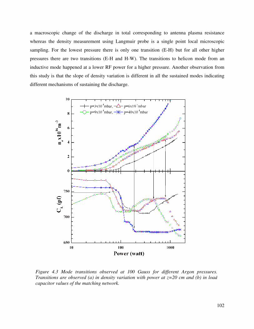
102
a macroscopic change of the discharge in total corresponding to antenna plasma resistance
whereas the density measurement using Langmuir probe is a single point local microscopic
sampling. For the lowest pressure there is only one transition (E-H) but for all other higher
pressures there are two transitions (E-H and H-W). The transitions to helicon mode from an
inductive mode happened at a lower RF power for a higher pressure. Another observation from
this study is that the slope of density variation is different in all the sustained modes indicating
different mechanisms of sustaining the discharge.
Figure 4.3 Mode transitions observed at 100 Gauss for different Argon pressures.
Transitions are observed (a) in density variation with power at z=20 cm and (b) in load
capacitor values of the matching network.

103
However, from all these above-mentioned observations we can conclude that at low powers (<
50 W) the plasma discharges are capacitive in nature i.e. the power is coupled to the plasma
capacitively. As we increased the input power > 50 W up to < 500 W, the power is coupled to
the plasma inductively and higher densities compared to the capacitive mode are observed. At
higher powers (> 500W), the power coupling to the plasma happens due to the direct coupling of
antenna fields to helicon wave fields as the density rises more sharply compared to the inductive
mode.
The existence of inductive and helicon modes are further supported by the measurement of
density profile at 22 cm away from the source as it is expected that for an inductive mode the
power deposition will be away from the center and near the boundary unlike the helicon mode in
which maximum power is deposited away from the radial boundary of the discharge [4, 9-10].
Figure 4.4 Radial density profile for two different RF powers (50Wand 600W)
at pressure ∼2 × 10⁻³
mbar and magnetic field ∼100 G measured at Z=22 cm.

104
At low input power (~ 50 - 500 W), radial profile of electron density remains hollow (Figure
4.4), a signature of inductive mode discharge. However, at higher input power (>500 W) peaked
radial profile of density is observed (Figure 4.4), indicating the existence of helicon mode in the
plasma.
4.3 Mode structure at Low magnetic field
Excitation of helicon = +1 mode is confirmed by measuring the axial component of
wave magnetic field along the radius. Figure 4.x shows the variation Bz amplitude normalized to
unity, measured with a single loop B-dot probe at z = 22 cm with 300 W RF power and 2 ×10 . !"# pressure. Along with are shown theoretical = +1 curves of Bz of helicon waves
in a cylindrical boundary [24] with a perpendicular wave number of 76 m-1.
Figure 4.5Radial variation measured Bz (circles) at 30 G, 300W and 2 × 10⁻³
mbar. The
solid lines are theoretical curves of pure = + mode along with mixed modes with 25%,
50%, 75% and 100% additional = mode content. All values are normalized to 1.
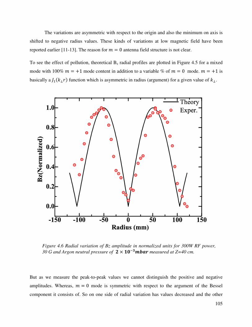
105
The variations are asymmetric with respect to the origin and also the minimum on axis is
shifted to negative radius values. These kinds of variations at low magnetic field have been
reported earlier [11-13]. The reason for = 0 antenna field structure is not clear.
To see the effect of pollution, theoretical Bz radial profiles are plotted in Figure 4.5 for a mixed
mode with 100% = +1 mode content in addition to a variable % of = 0 mode. = +1 is
basically a W,(K¿#) function which is asymmetric in radius (argument) for a given value of K¿.
But as we measure the peak-to-peak values we cannot distinguish the positive and negative
amplitudes. Whereas, = 0 mode is symmetric with respect to the argument of the Bessel
component it consists of. So on one side of radial variation has values decreased and the other
Figure 4.6 Radial variation of Bz amplitude in normalized units for 300W RF power,
30 G and Argon neutral pressure of × measured at Z=40 cm.

106
side the values are increased, the total radial variation which on normalization gives an
asymmetrical behavior.
Though it is expected that the induced fields (or antenna fields) will die down in a thin skin
depth, the application of magnetic field has already been proposed by Chen [14] to increase the
skin depth giving rise to an anomalous skin depth.
Figure 4.5 shows that a pollution of ~ 25% = 0 mode is there. To confirm that the antenna
fields are causing the asymmetric radial variation, Bz in the downstream plasma is measured at
z=40 cm. Figure 4.6 shows a radial profile which is symmetric which confirms that = 0 mode
pollution is negligible. So, the mode structure measured near the antenna shows = +1 mode
Figure 4.7 Variation of axial magnetic field of Helicon wave along the axis for 600
W RF power at pressure ~ 2 x 10⁻³
mbar and magnetic field ~ 100 Gauss.

107
excitation with pollution from = 0 mode with a pure = +1 mode downstream of the
source.
The existence of helicon wave in the plasma at higher input powers (>500 W) is further
substantiated by the measurement of axial profile of wave magnetic field using a single loop B-
dot probe as shown in Figure 4.7 for 600 W RF power and a pressure of 2 x 10⁻³ mbar with 100
Gauss magnetic field . From the slope of the axial phase variation of the wave magnetic field, the
wavelength was calculated ~ 22 cm in the source region and ~19.5 cm in the diffusion region
using the phase axial slope as shown from Figure 4.8.
4.4 Axial density profile
One of the primary aims of this thesis is study of CFDL. CFDL in a helicon discharge are
typically performed in an expanding geometry and an expanding magnetic field with 100’s of
Gauss in the source chamber and 10’s of Gauss in the diffusion chamber [15-19]. The combined
Figure 4.8 Axial variation of helicon wave phase measured at r=0 with a single
loop B-dot probe at ∼2 × 10⁻³
mbar, 300W and 100 G magnetic field.

108
effect of both geometry and magnetic field expansion sets up a density gradient in the axial
direction which gives rise to an ambipolar potential drop. This potential drop evolves into a free
standing often stable potential structure as the neutral pressure is reduced. An experiment is
performed to look for density gradients set up in the axial direction at 2 × 10 . mbar and 110
Gauss magnetic field near the antenna. Figure 4.8 shows axial variation of density measured by a
double Langmuir probe for three different powers at r = 0.
Upstream-to-downstream density ratios of ~ 2.7, 5.3 and 8.8 are obtained for RF input power of
200 W, 300 W and 400 W respectively. The variation of upstream and downstream densities
shows that the maximum power deposition is happening near the source only. But one of the
interesting features is a hump in the density near axial locations of z = 35-55 cm in the diffusion
chamber, the hump getting peaked for higher RF powers. Though the occurrence of downstream
density peaks much away from the antenna are reported in high power and high magnetic field
Figure 4.9 Axial variation of density measured at r=0 for three powers 200W,
300W and 400W, source magnetic field of 100 G and × mbar Ar pressure.

109
experiments [20-22], these downstream density peaks which are observed here at low magnetic
field low RF power are not reported so far. Thorough investigation of these downstream density
peaks will be discussed in Chapter 5.
4.5 Observation of Current free double layer
CFDL formation in the expanding helicon plasma is studied at 600W RF power, 280 G
magnetic field and Argon neutral pressure of 1.2 × 10 mbar. On axis plasma potential is
measured along the axial direction with a saturated emissive prove in floating potential method
(discussed in chapter 3) by passing a filament current of 2.7 Ampere in a 0.125 mm tungsten
filament. The variation of plasma potential and density are shown in Figure 4.3 (a) and (b)
respectively. The axial magnetic field profile used for this experiment is shown in Figure 3.3.
Figure 4.10 Axial variations of (a) plasma potential and (b) plasma density at × and . × of Argon with RF power of 600W and
280 G magnetic field in source.

110
Plasma expansion leads to a density fall with upstream and downstream densities of 5.5 ×10,</m3 and 1.7 × 10,</ m3 respectively with a nearly equal temperature of î( ~ 6 eV in the
potential fall region. The axial density is measured by a double probe and electron temperature is
measured by a RF compensated Langmuir probe. For this expansion to be a Boltzmann
expansion which relates upstream (n0, V0) and downstream (nz, Vz) densities and plasma
potentials by ól − ó; = −î( (<ó) × =(l ;⁄ ) [15, 17, 23], the maximum drop should be ~ 7.5
V. This observation plasma potential drop of ~ 50 V in bulk plasma is more than the local î( can
be termed as a CFDL as it cannot be explained through a simple Boltzmann plasma expansion.
The average thickness of the CFDL is ~ 1000 Q> taking into consideration of upstream and
downstream plasma density and electron temperature.
Measurement of density and plasma potential at a higher pressure of 2 × 10 . mbar is presented
in Figure 4.3 (a) and (b) respectively where a potential drop of ~ 6 V is observed which is of the
order of the local electron temperature of ~ 5 eV and for this the expected plasma potential drop
due to a Boltzmann plasma expansion is ~ 4.4 V.
So, we have observed a CFDL in the source chamber plasma before the geometrical expansion
into the diffusion chamber with a potential drop ?>«~8î( and thickness of ~ 1000 Q> which
form at low pressure and are not observed at higher pressure. Though this kind of CFDL with
thickness > 50-100 Q> are observed in few recent experiments [15-16], there are experiments
with observation of sharp CFDL with thickness < 100 Q> [17-19]. Further studies on sharp
CFDL formation and the effect of magnetic field gradient will be presented in Chapter 6.
4.6 Summary of Chapter 4
Antenna resistance is measured without plasma. Helicon antenna efficiency is shown to
increase with RF power in the presence of plasma. Discharge mode transitions are observed at
different pressures. At lower pressure the transitions are obtained at higher RF powers for a
constant magnetic field. Radial density profiles are shown to confirm the inductive and helicon
modes. Helicon wave excitation with half helical = +1 mode is confirmed by measuring the
radial variation of the axial component of magnetic field. Additionally, the mode is shown to be

111
polluted by the antenna fields near the antenna and pure away from the antenna in the diffusion
chamber. Axial variation of the phase of the helicon wave gives a wave length of 22 cm in the
source and 19.5 cm in the diffusion chamber. Axial density profiles in a diverging magnetic field
configurations shows upstream-to-downstream density ratios of ~ 2.7, 5.3 and 8.8 are obtained
for RF input power of 200 W, 300 W and 400 W respectively. Downstream density peaks are
observed in the diffusion chamber which gives indication of helicon power deposition away from
the antenna. Current free double layer is observed at low pressures with a potential drop of ~ 8
kTe/e and thickness of ~ 1000 Q>. The double layer vanished at higher pressure with the potential
drop of the order of Te and can be explained through a simple Boltzmann expansion. The DL is
formed inside the source chamber and in the bulk of the plasma aligned to magnetic field.
112
References
[1] Chi, Kyeong-Koo, T. E. Sheridan, and R. W. Boswell. "Resonant cavity modes of a bounded helicon discharge." Plasma Sources Science and Technology 8, no. 3 (1999): 421.
[2] Lafleur, T., C. Charles, and R. W. Boswell. "Characterization of a helicon plasma source in low diverging magnetic fields." Journal of Physics D: Applied Physics 44.5 (2011): 055202.
[3] Ellingboe, A. R., and R. W. Boswell. "Capacitive, inductive and helicon‐wave modes of operation of a helicon plasma source." Physics of Plasmas 3 (1996): 2797.
[4] Franck, Christian M., Olaf Grulke, and Thomas Klinger. "Mode transitions in helicon discharges." Physics of Plasmas 10 (2003): 323.
[5] Boswell, R. W. "Very efficient plasma generation by whistler waves near the lower hybrid frequency." Plasma Physics and Controlled Fusion 26.10 (1984): 1147.
[6] Perry, A. J., D. Vender, and R. W. Boswell. "The application of the helicon source to plasma processing." Journal of Vacuum Science & Technology B: Microelectronics and Nanometer
Structures 9, no. 2 (1991): 310-317.
[7] Perry, Andrew, Garrard Conway, Rod Boswell, and Harold Persing. "Modulated plasma potentials and cross field diffusion in a Helicon plasma." Physics of Plasmas 9 (2002): 3171.
[8] Chi, Kyeong-Koo, T. E. Sheridan, and R. W. Boswell. "Resonant cavity modes of a bounded helicon discharge." Plasma Sources Science and Technology 8, no. 3 (1999): 421.
[9] Degeling, A. W., C. O. Jung, R. W. Boswell, and A. R. Ellingboe. "Plasma production from helicon waves." Physics of Plasmas 3 (1996): 2788.
[10] Yun, Seokmin, Suwon Cho, George Tynan, and Hongyoung Chang. "Density enhancement near lower hybrid resonance layer in m= 0 helicon wave plasmas." Physics of Plasmas 8 (2001): 358.
[11] Sato, Genta, Wataru Oohara, and Rikizo Hatakeyama. "Experimental evidence of m=-1 helicon wave cutoff in plasmas." Journal of the Physical Society of Japan 75.4 (2006): 3501.
[12] Chi, Kyeong-Koo, T. E. Sheridan, and R. W. Boswell. "Resonant cavity modes of a bounded helicon discharge." Plasma Sources Science and Technology 8.3 (1999): 421.
[13] Lafleur, T., C. Charles, and R. W. Boswell. "Plasma control by modification of helicon wave propagation in low magnetic fields." Physics of Plasmas 17 (2010): 073508.
[14] Chen, Francis F. "Collisional, magnetic, and nonlinear skin effect in radio-frequency plasmas." Physics of Plasmas 8 (2001): 3008.
[15] Charles, Christine, and Rod Boswell. "Current-free double-layer formation in a high-density helicon discharge." Applied Physics Letters 82, no. 9 (2003): 1356-1358.

113
[16] Sutherland, Orson, Christine Charles, N. Plihon, and R. W. Boswell. "Experimental evidence of a double layer in a large volume helicon reactor." Physical review letters 95, no. 20 (2005): 205002.
[17] Takahashi, K., K. Oguni, H. Yamada, and T. Fujiwara. "Ion acceleration in a solenoid-free plasma expanded by permanent magnets." Physics of Plasmas 15 (2008): 084501.
[18] Hairapetian, G., and R. L. Stenzel. "Expansion of a two-electron-population plasma into vacuum." Physical review letters 61, no. 14 (1988): 1607.
[19] Sun, Xuan, Amy M. Keesee, Costel Biloiu, Earl E. Scime, Albert Meige, Christine Charles, and Rod W. Boswell. "Observations of ion-beam formation in a current-free double layer." Physical review letters 95, no. 2 (2005): 025004.
[20] Chen, Francis F., Isaac D. Sudit, and Max Light. "Downstream physics of the helicon discharge." Plasma Sources Science and Technology 5.2 (1996): 173.
[21] Chen, Francis F. "Physics of helicon discharges." Physics of Plasmas 3 (1996): 1783.
[22] Sudit, Isaac D., and Francis F. Chen. "Discharge equilibrium of a helicon plasma." Plasma
Sources Science and Technology 5.1 (1996): 43.
[23] Wiebold, Matt, Yung-Ta Sung, and John E. Scharer. "Experimental observation of ion beams in the Madison Helicon eXperiment." Physics of Plasmas 18 (2011): 063501.
[24] Chen, Francis F. "Plasma ionization by helicon waves." Plasma Physics and Controlled
Fusion 33.4 (1991): 339.
114
Chapter 5
Low Magnetic Field Helicon Studies
5.1 Introduction
A Helicon source operates in the frequency range between ion cyclotron and electron
cyclotron frequencies usually with magnetic field of few hundreds of Gauss to few kilo Gauss.
Appearance of helicon mode is generally identified by mode transitions which involves a
transition from a capacitive to inductive to wave sustained discharge [1]. The transitions are can
be observed from the step like transitions in measured plasma density and antenna-plasma
coupling, obtained by increasing power at fixed magnetic field (B) of few hundred Gauss or
vice versa. At high magnetic fields (>100 Gauss) it is observed that the density increases with
applied magnetic field when in helicon mode as per the dispersion relation. However, previous
studies have shown that at low magnetic fields of less than 100 Gauss, plasma density peaks at
some specific magnetic fields, generally between 20 Gauss to 50 Gauss in different experiments
using 13.56 MHz RF system [2-9]. Unlike usual helicon discharge mode transitions (see Chapter
2 and 4) at high magnetic fields (few hundred Gauss), the observance of density peaks at low
magnetic fields seems to be a resonance phenomenon.
Chen [3] first reported this low magnetic peak in 2 cm diameter helicon discharge using
1600 W RF power where the density peak was observed at ~ 50 G with peak density of 6 ×10,- . an increase of nearly 40% from the no field case. Many other experiments
subsequently reported similar observations of a density peak at magnetic fields between 10-50 G.
Degeling et al [2] have observed density peak (Figure 5.1) around 50G for RF powers in 500-
2000 W in a 18 cm diameter source using single loop antenna at 13.56 MHz. Wang et al have
shown that the a higher magnetic field is required for the density peak to occur for a plasma

formed using higher ion mass or a higher source frequency. He measured the plasma resistance
and has shown that the plasma resistance is wel
An experiment by Eom [10] has shown that for a high frequency RF discharge operating
at 98 MHz, the peak occurs at 140 G. Recently Lafleur et al [9] have done extensive experiments
in a diverging magnetic field helicon experiment and shown that the density
order from the no field case. Their density variations were well correlated with the measured
variations of antenna-plasma radiation resistance and Q
powers and pressures in a helicon discharge p
Very few explanations are available for the observed density peak at low magnetic
fields. Degeling et al [2] and Lafleur et al [9] interpreted this by invoking wave particle trapping;
however the dependence of the
mentioned of a direct transition from a capacitive discharge at no applied magnetic field to a
helicon discharge at the peak magnetic field (where the density peaks). But it is not clear why
discharge is not maintained for magnetic fields higher than the peak magnetic field and transits
back to a capacitive discharge. Chen
(m = 0) antenna that the density peak at low magnetic field
between m = +1 mode propagating along the magnetic field and the m = +1 mode generated due
the source end wall reflection of m =
Figure 5.8 Density variation with applied magnetic field in the
WOMBAT experiment. Degeling et al [
formed using higher ion mass or a higher source frequency. He measured the plasma resistance
and has shown that the plasma resistance is well correlated with the density variations.
An experiment by Eom [10] has shown that for a high frequency RF discharge operating
at 98 MHz, the peak occurs at 140 G. Recently Lafleur et al [9] have done extensive experiments
in a diverging magnetic field helicon experiment and shown that the density can increase by an
order from the no field case. Their density variations were well correlated with the measured
plasma radiation resistance and Q-value of the RF circuit for different RF
powers and pressures in a helicon discharge produced by a double-saddle coil antenna.
Very few explanations are available for the observed density peak at low magnetic
fields. Degeling et al [2] and Lafleur et al [9] interpreted this by invoking wave particle trapping;
trapping on magnetic field is not clear. Lafleur et al have also
mentioned of a direct transition from a capacitive discharge at no applied magnetic field to a
helicon discharge at the peak magnetic field (where the density peaks). But it is not clear why
discharge is not maintained for magnetic fields higher than the peak magnetic field and transits
back to a capacitive discharge. Chen [11] suggested through the HELIC code results for a loop
(m = 0) antenna that the density peak at low magnetic field is due to the constructive interference
between m = +1 mode propagating along the magnetic field and the m = +1 mode generated due
the source end wall reflection of m = -1 mode propagating opposite to the magnetic field
Density variation with applied magnetic field in the
WOMBAT experiment. Degeling et al [2].
115
formed using higher ion mass or a higher source frequency. He measured the plasma resistance
l correlated with the density variations.
An experiment by Eom [10] has shown that for a high frequency RF discharge operating
at 98 MHz, the peak occurs at 140 G. Recently Lafleur et al [9] have done extensive experiments
can increase by an
order from the no field case. Their density variations were well correlated with the measured
value of the RF circuit for different RF
saddle coil antenna.
Very few explanations are available for the observed density peak at low magnetic
fields. Degeling et al [2] and Lafleur et al [9] interpreted this by invoking wave particle trapping;
trapping on magnetic field is not clear. Lafleur et al have also
mentioned of a direct transition from a capacitive discharge at no applied magnetic field to a
helicon discharge at the peak magnetic field (where the density peaks). But it is not clear why the
discharge is not maintained for magnetic fields higher than the peak magnetic field and transits
[11] suggested through the HELIC code results for a loop
is due to the constructive interference
between m = +1 mode propagating along the magnetic field and the m = +1 mode generated due
1 mode propagating opposite to the magnetic field
Density variation with applied magnetic field in the

116
direction. The axial power absorption was shown to be in the near field of the antenna and the
radial power absorption was near the plasma boundary. This radial boundary power absorption
was shown to be due to TG modes. Again, it is not clear why the reflection occurs only at certain
low magnetic fields and why similar density peak is not observed for high magnetic fields.
Shamrai and Taranov [12] analytically derived the wave dispersion relation for waves
propagating parallel to the magnetic field in a bounded plasma medium taking into account the
finite mass of electrons. They found that the wave dispersion relation has two modes, one
helicon (fast) and other is TG (slow) mode. Furthermore, they have predicted the possibility of
mode conversion from helicon to TG mode in helicon plasmas. These two modes are well
separated at higher magnetic field (> 200 Gauss for 13.56 MHz); however at low magnetic fields
(< 100 Gauss for 13.56 MHz) they get coupled naturally under some typical conditions. Later
Cho [13] studied the dispersion characteristics of the radial eigenmodes and resistive loading of
helicon plasmas to explain the occurrence of the density peak at low magnetic fields. He
concluded that in case of helical antenna the occurrence of density peaks are due to TG-helicon
mode coupling at specific low magnetic fields where the perpendicular wave numbers of the
helicon and TG modes are equal. Though TG modes are detected indirectly by Blackwell et al
[14], their direct absorption has not been measured.
Most of the works at low magnetic field helicon discharges have shown a density peak away
from the ECR magnetic filed ~5 G for 13.56 MHz source frequency. In this thesis for the first
time experimental observation of two density peaks (excluding the ECR peak) are reported in a
helicon discharge carried out in low magnetic field (< 100 Gauss). The occurrence of density
peaks is explained with the help of resonance of obliquely propagating right circular polarized
electromagnetic (helicon) wave. These results are discussed in section 5.2. Plasma density and
visible light intensity are measured on both sides of the antenna along with the antenna plasma
resistance to look for the role of m = -1 modes. The observations and explanations are discussed
in Section 5.3 in the light of polarization reversal of = ±1 modes. Some of the high uniform
magnetic field helicon discharge experiments have shown the peaking in axial density away from
the helicon antenna. But with a low diverging magnetic field downstream density peaks have
been observed nearly two wavelengths away from the antenna centre. This results on
downstream density peaking are discussed in Section 5.4 for different RF power and neutral gas
pressure. Though all the experiments of low field density peak are done earlier by many authors

117
in uniform magnetic fields the recent results by Lafleur et al [9] shows that a for a single coil
near the antenna the density rises nearly ten times. So, the density peaking phenomena along
with the antenna-plasma coupling is studied for four different magnetic field topologies near the
antenna and will be discussed in Section 5.5.
5.2 Multiple Density Peaks
After achieving a base pressure of ~ 1 x 10⁻⁶ mbar in the system, argon gas is fed into the system
at different pressures to produce plasma by powering the helicon antenna. The plasma density is
measured using a double Langmuir probe placed in the source chamber 20 cm away from
antenna centre towards the diffusion chamber. Figure 5.2 shows variation of measured axial
plasma electron density at z = 22 cm with applied magnetic field near the antenna in the source
chamber for different RF power and pressure. As the magnetic field is slowly increased from 0
G, the density also increases and goes through the ECR point around 5 G. Beyond the ECR point
density continues to increase monotonically till 25 G to 30 G before falling sharply to half of its
peak value near 40 G. However, increasing the magnetic field above 40 G, the density again
increases and attains a peak around 50 G. It is clear from the figure that the magnitude of the
main density peak at ~ 25 G increases with both pressure and power. Density rises approximately
three times from 6 x 10¹⁶m
-3 to a peak value of ~2 x 10¹⁷m
-3 at higher pressures (~ 2 x 10⁻³mbar).
Whereas, at lower pressure of ~0.4 x 10⁻³mbar, density only rises to ~ 40% of its initial value.
The second peak is much clearly visible at low fill-in pressures. Figure 5.2 further shows that the
main density peak always occurs at magnetic field values between 20 G to 30 G with the peak
shifting towards the higher magnetic fields for higher power and pressure much like other
reported results at low magnetic fields [7,9]. This kind of resonance density peaking with
magnetic field seems likely to be the result of wave coupling rather than transitions of EHW
type.

118
Figure 5.3 shows the variation of matching network CL values for corresponding values of RF
power, fill-in pressure and magnetic field for which density is measured (Figure 5.2). The CL
values, as mentioned in Chapter 3 are measure of the antenna-plasma coupling (RP) through the
relation «Ã 1 ¡è⁄ . So a dip in CL value is indicative of a peak in RP. Multiple RP peaks in
magnetic fields can be deciphered from the « variations shown in the above figure consistent
with the corresponding density variations except at low RF power and low fill-in pressures.
Figure 5.3 CL values of the matching network at z = 20 cm versus magnetic field. (a) 300, 400, and
500 W RF power, p = 2 × 10⁻³ mbar, (b) 300, 400, and 500 W RF power, p = 0.8 × 10
−3 mbar, and
(c) 100, 200, and 350 W RF power, p = 0.4 × 10⁻³ mbar.
Figure 5.2 Plasma density on axis at z = 20 cm versus magnetic field. (a) 300, 400, and 500 W RF
power, p = 2 × 10⁻³ mbar, (b) 300, 400, and 500 W RF power, p = 0.8 × 10
−3 mbar, and (c) 100, 200,
and 350 W RF power, p = 0.4 × 10⁻³ mbar.

119
It should be noted that at low densities, the changes in RP are very less beyond the first peak, so
that the changes in « are not resolvable through the previously mentioned inverse square-root
dependence on RP. Another feature to be noted is that though « variations have appreciable
dips around 5 G for almost all the plots, the density variations do not show significant density
peaks.
The existence of the helicon wave is established in our experiment by measuring the amplitude
and phase of the axial wave magnetic field, Bz using a single loop B-dot probe. In Figure 5.6
magnitude of axial wave magnetic field along the z-axis is plotted for two different magnetic
fields (25 G and 50 G) where the 1st and 2nd density peaks are observed. The measurements are
done by positioning the magnetic probe 10 cm downstream from the antenna and moving it along
the z-axis for discharges with argon fill-in pressure of 0.4x10⁻³ mbar and 350 W RF power. As
seen from figure 5.4, a hump in Bz around 20-40 cm has been observed, which is because of
beating between the fundamental and higher order radial modes as established earlier [15-16].
The time difference between the reference probe and scanning probe gives the phase and the
phase variation as a function of distance is plotted in Figure 5.5 for B = 25 and 50 G.
Figure 5.4 Axial profile of the axial component of the wave
magnetic field at two different (30 and 50 G) ambient magnetic
fields.

120
The effective travelling wavelength is calculated from the slope of the fitted straight lines to the
experimental data using the expression Q∥=360(?/)−1, where z is the axial distance and φ is
the phase. Parallel wavelengths for B= 25 G and 50 G come out to be ~18 cm and 40 cm
respectively. Corresponding parallel wavenumbers are K∥ = 34 m-1 and K∥ = 15.7 m-1 and
parallel refractive indices (||) are 123 and 55 respectively.
Investigating the experimental results further, we revisited the wave properties of helicon
plasma. The relevant mode in helicon regime is the R-wave with $ ≪ $%( also known as the
whistler wave. Bounded whistler waves are referred as helicon waves. The dispersion relation for
R-wave in cold magnetized plasma can be rewritten as follows (Equation 2.61):
= %@>@@@ = 1 − @AB@@(@¯&C @DB%3eÏ) (5.1)
Figure 5.5 Variation of phase with distance for p = 0.4 × 10⁻³ mbar, RF power
350 W. B = 30 G (open circle) and B = 50 G (open diamond).

121
Where is the index of refraction, K = K∥ + K¿ , = K∥ K ⁄ with K, K∥ " K¿are
respectively total, parallel and perpendicular wavenumbers.$, $E< " $< are respectively the
wave, electron plasma and electron cyclotron frequencies, F is the electron collision frequency
and is the velocity of light. In the frequency range, $≪ $≤ $<≪$E<, the dispersion relation
becomes
%@>@@@ = @AB@@(@DB%3eÏ @ &C) (5.2)
This equation has two solutions for K. Since in helicon antenna produced plasma parallel
wavenumber K∥ is set by antenna so it may be wiser to consider rewriting the dispersion relation
in terms of K¿following Shamrai and Taranov [12]
K¿± = K∥ ,G@H@ c1 − 2Ã − 2ÃI ± √1 − 4Ãd (5.3)
Where,
à = $)($%( ∥ , I = $$%(∥$)(
The above equation shows that there are two values of K¿ related to slow and fast wave. K¿¯ corresponds to TG perpendicular wave number and K⊥− corresponds to helicon
perpendicular wave number. It is seen from equation 5.3 that necessary condition of propagation
of both the waves is à < 1 4 . <. , $)( < $ÎÔ? = (1 4⁄ )$%( ∥⁄ considering collisionless wave
propagation. In addition to this, the bracketed term in right hand side of Equation 5.3 should be
positive for helicon wave to propagate. This happens when I < 1 or $)( > $Î&J = $$%(∥. Hence, helicon wave propagates radially outward from higher to lower density with I ~1 and à = 1 4⁄ are the lower and higher cut-off conditions for helicon respectively. For plasmas with a
radial non-uniformity, helicon mode propagates in the interior of plasma where Ã<1/4 and
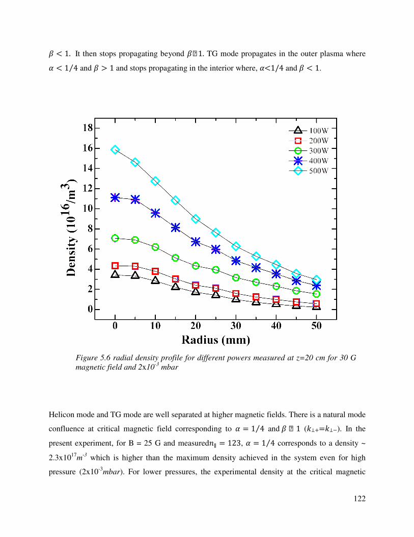
122
I < 1. It then stops propagating beyond I~1. TG mode propagates in the outer plasma where à < 1 4⁄ and I > 1 and stops propagating in the interior where, Ã<1/4 and I < 1.
Helicon mode and TG mode are well separated at higher magnetic fields. There is a natural mode
confluence at critical magnetic field corresponding to à = 1 4⁄ and I ~ 1 (K⊥+=K⊥−). In the
present experiment, for B = 25 G and measured∥ = 123, Ã = 1 4⁄ corresponds to a density ~
2.3x10¹⁷m
-3 which is higher than the maximum density achieved in the system even for high
pressure (2x10⁻³mbar). For lower pressures, the experimental density at the critical magnetic
Figure 5.6 radial density profile for different powers measured at z=20 cm for 30 G
magnetic field and 2x10⁻³
mbar

123
field is even lower. This means Ã=1/4 natural mode confluence point (high density cut-off for
helicon) does not exist in the system and hence TG-helicon coupling does not seem to explain
the observed density peaks in our experiment. Further the measured radial density profiles at z =
22 for different RF powers and fill-in pressure of 8x10⁻⁴ mbar as shown in Figure 5.6 does not
show any localized power absorption at the plasma boundary as observed in HELIC code
simulations by Chen [11].
The experimental evidence of presence of radial modes illustrates the possibility of obliquely
propagating helicon modes. Taking the mass of the electron ( = 0, the boundary condition for
helicon wave propagation gives the perpendicular wavenumbers for cylindrical plasma which
can be obtained by the zeros of the Bessel component of wave magnetic fields. For the first and
the second zeros of first order Bessel function (J1), K¿, and K¿ are given by 3.83/" and 7.02 "⁄
respectively where " is the effective plasma radius. Taking " = 5 in our case, we get K⊥1∼76 −1 and K¿ ∼ 140 ,. Similar values of k¿ are reported in similar experimental setup and
conditions by Lafleur et al [9, 17]. Once the K∥ " K⊥ are known, the angle of propagation can
be found from the expression = K∥ K⁄ = K∥ LK∥ + K¿È . To understand the relation
between the angle of propagation and critical magnetic field where density peaks let us look into
the resonance cone behaviour of obliquely propagating helicon wave. For obliquely propagating
R-wave, the cold plasma dispersion relation following Stix’s notation can be written as
g" = − è(J@ )(J@ «)M(J@ «)(J@ è) (5.4)
Where n is the refractive index and coefficients P, R, L and S are given in reference 18.
At resonance, ( → ∞), this requires,
g"N(e = − èM (5.5)
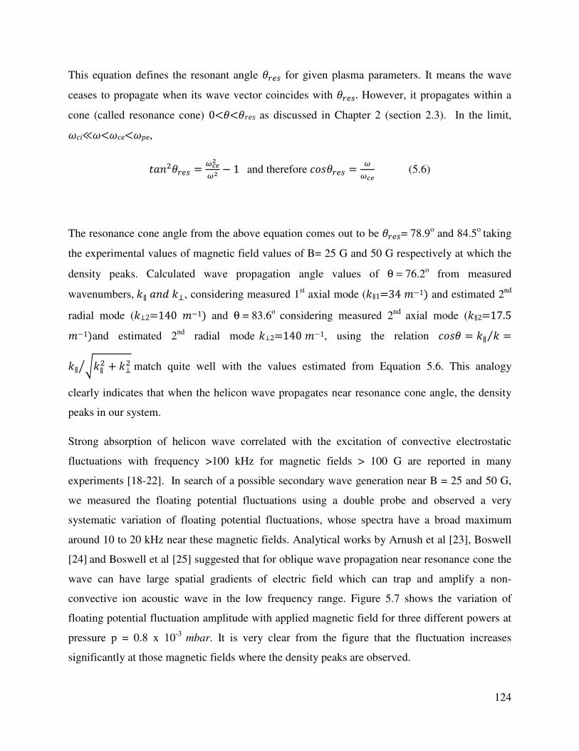
124
This equation defines the resonant angle N(e for given plasma parameters. It means the wave
ceases to propagate when its wave vector coincides with N(e. However, it propagates within a
cone (called resonance cone) 0<<#< as discussed in Chapter 2 (section 2.3). In the limit, $≪$<$<<$E<, g"N(e = @DB@@@ − 1 and therefore N(e = @@DB (5.6)
The resonance cone angle from the above equation comes out to be N(e= 78.9o and 84.5o taking
the experimental values of magnetic field values of B= 25 G and 50 G respectively at which the
density peaks. Calculated wave propagation angle values of θ = 76.2o from measured
wavenumbers, K∥ " K¿, considering measured 1st axial mode (K∥1=34 −1) and estimated 2nd
radial mode (K⊥2=140 −1) and θ = 83.6o considering measured 2nd axial mode (K∥2=17.5 −1)and estimated 2nd radial mode K⊥2=140 −1, using the relation = K∥ K⁄ =K∥ LK∥ + K¿È match quite well with the values estimated from Equation 5.6. This analogy
clearly indicates that when the helicon wave propagates near resonance cone angle, the density
peaks in our system.
Strong absorption of helicon wave correlated with the excitation of convective electrostatic
fluctuations with frequency >100 kHz for magnetic fields > 100 G are reported in many
experiments [18-22]. In search of a possible secondary wave generation near B = 25 and 50 G,
we measured the floating potential fluctuations using a double probe and observed a very
systematic variation of floating potential fluctuations, whose spectra have a broad maximum
around 10 to 20 kHz near these magnetic fields. Analytical works by Arnush et al [23], Boswell
[24] and Boswell et al [25] suggested that for oblique wave propagation near resonance cone the
wave can have large spatial gradients of electric field which can trap and amplify a non-
convective ion acoustic wave in the low frequency range. Figure 5.7 shows the variation of
floating potential fluctuation amplitude with applied magnetic field for three different powers at
pressure p = 0.8 x 10⁻³ mbar. It is very clear from the figure that the fluctuation increases
significantly at those magnetic fields where the density peaks are observed.

125
Therefore, oblique helicon wave propagation along the resonance cone boundary in this
experiment seems to be generating a non-convective electrostatic wave, which is transferring the
energy to the plasma from helicon waves creating density peaks at specific magnetic fields and
hence describes the dependence of density peaking at those specific magnetic fields.
Further, the observed dependency of density peak occurrences at specific magnetic fields on
source frequency with similar conditions of RF power, neutral pressure, source tube radius and
antenna in reference 7 (Figure 6) can easily be explained using our model as keeping the RF
power, neutral pressure, source tube radius and antenna same, the ratio of K∥ K⁄ remains
constant, and to satisfy the resonance cone propagation condition expressed in Equation 5.6, the
density peak should occur at higher magnetic fields for a higher source frequency.
Figure 5.7 Floating potential fluctuation amplitude variation with magnetic field measured
for RF powers of 200 W, 300 W and 400 W with argon fill in pressure of 0.8 × 10⁻³
mbar.

126
5.3 Polarization reversal and asymmetric density peaking
Lot of studies has been carried out to understand the density peak at low B away from
ECR point in helicon plasmas. One of the interesting observations of last section (Figure 5.2 and
Figure 5.3) is that the capacitance values have large dips around 5 Gauss but the density plots do
not show peaks ~ 5 Gauss. As mentioned earlier, the CL values are measure of plasma resistance
and show the macroscopic behavior of the plasma. The source frequency of 13.56 MHz
corresponds to the electron cyclotron resonance (ECR) for magnetic field ~ 5 Gauss. The
observation of non-absorption of ECR wave is anti-intuitive. One of the possible reasons may be
polarization reversal. The electromagnetic wave propagating along the direction of magnetic
field is a right hand polarized wave (RHPW) and that propagating in a direction opposite to
magnetic field is left hand polarized wave (LHPW). The polarization of the launched mode is
maintained only at the axis and the boundary condition (:Ï = 0) for a bounded wave needs the
wave to have a linear polarization. This process is shown theoretically and experimentally for
microwave frequencies for electron cyclotron waves that an LHPW can have its polarization
reversed to an RHPW or vice versa in bounded plasmas.
However, not much literature is available for the process of polarization reversal in range of
radio frequencies. As it is a well-known fact that the right polarized wave should be absorbed
near the ECR point, however, the small or nonexistent density peak near ECR point observed in
the previous helicon experiments warrants detailed studies. Lafleur et al [9] reported that the
peaking phenomenon is magnetic field direction independent. Parametric studies are carried out
by changing both the magnetic field magnitude and direction at different powers and pressures.
The magnetic field direction along the positive z-axis is referred to as “normal B direction” and
“m = ±1 sides” is referred to the sides towards which the conventional m = ±1 helicon modes
propagate (Figure 5.8).
The plasma density is measured by a movable double Langmuir probe (DP) and an RF
compensated Langmuir probe, which is also used for temperature measurement. Two collimated
optical probes (lens-fiber combination) are used to collect the visible light from the same
locations that of the Langmuir probes and transmitted to photodiodes through optical fibers and
subsequently converted to voltage signals by current to voltage converters. A Pearson make
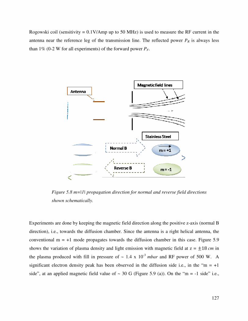
Rogowski coil (sensitivity = 0.1V/Amp up to 50 MHz) is
antenna near the reference leg of the transmission line. The reflected power
than 1% (0-2 W for all experiments) of the forward power
Experiments are done by keeping the magnetic field direction along the positive z
direction), i.e., towards the diffusion chamber. Since the antenna is a right helical antenna, the
conventional m = +1 mode propagates towards the diffusion chamber in this case. Figure 5.9
shows the variation of plasma density and light emission with magnetic field at z =
the plasma produced with fill in pressure of ~ 1.4 x 10
significant electron density peak has been observed in the diffusion side i.e., in the “m = +1
side”, at an applied magnetic field value of ~ 30 G (Figure 5.9 (a)). On the “m =
Figure 5.8 m=|1| propagation direction for
shown schematically.
Rogowski coil (sensitivity = 0.1V/Amp up to 50 MHz) is used to measure the RF current in the
antenna near the reference leg of the transmission line. The reflected power P
2 W for all experiments) of the forward power PF.
Experiments are done by keeping the magnetic field direction along the positive z
direction), i.e., towards the diffusion chamber. Since the antenna is a right helical antenna, the
conventional m = +1 mode propagates towards the diffusion chamber in this case. Figure 5.9
shows the variation of plasma density and light emission with magnetic field at z =
the plasma produced with fill in pressure of ~ 1.4 x 10⁻³ mbar and RF power of 500 W. A
significant electron density peak has been observed in the diffusion side i.e., in the “m = +1
side”, at an applied magnetic field value of ~ 30 G (Figure 5.9 (a)). On the “m =
Figure 5.8 m=|1| propagation direction for normal and reverse field directions
shown schematically.
127
used to measure the RF current in the
PR is always less
Experiments are done by keeping the magnetic field direction along the positive z-axis (normal B
direction), i.e., towards the diffusion chamber. Since the antenna is a right helical antenna, the
conventional m = +1 mode propagates towards the diffusion chamber in this case. Figure 5.9
shows the variation of plasma density and light emission with magnetic field at z = ±18 cm in
and RF power of 500 W. A
significant electron density peak has been observed in the diffusion side i.e., in the “m = +1
side”, at an applied magnetic field value of ~ 30 G (Figure 5.9 (a)). On the “m = -1 side” i.e.,
normal and reverse field directions

128
towards the source end plate side, density peaks are distinctively different compared to the “m =
+1 side” both in terms of magnitude and required magnetic fields as shown in Figure 5.9 (b).
Figure 5.9 Variation of electron density (ne), visible light intensity (Ivis) and
antenna plasma resistance (Rp) with magnetic field for 500 W at pressure
1.4x10⁻³
mbar. (a) ne at +18 cm, (b) ne at -18 cm, (c) Ivis at +18 cm, (d) Ivis at -
18 cm and (e) Rp

129
In contrast to the “m = +1 side” a very prominent density peak has been observed at 5 G which
corresponds to the electron cyclotron peak. Another peak in density has been observed around 12
G and a tiny hump in density around 50 G. In this “m = -1 side”, not only the density peak
around 30 G is absent, a decrease in density has been observed at this magnetic field. Further,
the magnitude of density peak on “m = -1 side” around 12 G is almost 1.5 times higher than the
density peak observed at ~ 30 G in the “m = +1 side”. The density data on either side is further
substantiated by recording the collimated total light emission from z = ±18cm as shown in
Figure 5.9(c) and 5.9(d). The light intensity variations closely follow the ion saturation current
variations on the respective sides for all RF powers and this non-intrusive method removes any
doubt regarding contamination of results due to the disturbances created by the Langmuir probes.
The characteristics behavior of density in the “m = +1 side” with the magnetic field direction
towards the same side, shows features similar to those described in Section 5.2. The variation of
Figure 5.10 Variation of electron density (ne) with magnetic field for 300, 400
and 500 W at pressure 1.4x10⁻³
mbar. (a) ne at +18 cm and (b) ne at -18 cm.

antenna plasma resistance, RP with the applied magnetic field is shown in Figure 5.9 (e). The
measurement clearly shows that the variatio
light emission measured at either side of the antenna. However, the sum of variations of plasma
density or total light emission from both sides of the antenna matches quite well with
quite expected, as RP is the macroscopic response of the plasma produced on both sides of the
antenna. So, the discrepancy observed in last section about the C
ECR peak on m =+1 side is understood now.
In order to establish the results further, the experiments are repeated for three different values of
fill in pressures as well as for three different values of input powers. The density and total light
Figure 5.11 Variation of electron density (n
pressures 8x10⁻⁴
, 1.4x10
with the applied magnetic field is shown in Figure 5.9 (e). The
measurement clearly shows that the variation of RP does not follow the plasma density or total
light emission measured at either side of the antenna. However, the sum of variations of plasma
density or total light emission from both sides of the antenna matches quite well with
is the macroscopic response of the plasma produced on both sides of the
antenna. So, the discrepancy observed in last section about the CL dips and no-occurrence of 5 G
ECR peak on m =+1 side is understood now.
In order to establish the results further, the experiments are repeated for three different values of
ill in pressures as well as for three different values of input powers. The density and total light
Variation of electron density (ne) with magnetic field for 500 W at
10-3
and 2.4x10⁻³
mbar. (a) ne at +18 cm, (b) ne at
130
with the applied magnetic field is shown in Figure 5.9 (e). The
does not follow the plasma density or total
light emission measured at either side of the antenna. However, the sum of variations of plasma
density or total light emission from both sides of the antenna matches quite well with RP. This is
is the macroscopic response of the plasma produced on both sides of the
occurrence of 5 G
In order to establish the results further, the experiments are repeated for three different values of
ill in pressures as well as for three different values of input powers. The density and total light
) with magnetic field for 500 W at
at -18 cm.
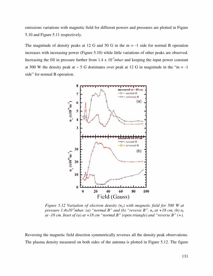
131
emissions variations with magnetic field for different powers and pressures are plotted in Figure
5.10 and Figure 5.11 respectively.
The magnitude of density peaks at 12 G and 50 G in the m = -1 side for normal B operation
increases with increasing power (Figure 5.10) while little variations of other peaks are observed.
Increasing the fill in pressure further from 1.4 x 10⁻³mbar and keeping the input power constant
at 500 W the density peak at ~ 5 G dominates over peak at 12 G in magnitude in the “m = -1
side” for normal B operation.
Reversing the magnetic field direction symmetrically reverses all the density peak observations.
The plasma density measured on both sides of the antenna is plotted in Figure 5.12. The figure
Figure 5.12 Variation of electron density (ne) with magnetic field for 500 W at
pressure 1.4x10⁻³
mbar. (a) “normal B” and (b) “reverse B”. ne at +18 cm, (b) ne
at -18 cm. Inset of (a) at +18 cm “normal B” (open triangle) and “reverse B” (+).

132
clearly shows that the density peak at ~ 30 G is now observed on the other side of the antenna
(towards the end plate) as the conventional “m = +1” mode now lies in this direction after
changing the magnetic field direction. Similarly the prominent density peak at ~ 5 G is observed
at positive z direction (towards diffusion chamber) as the “m = -1” mode now lies on this side.
By changing the magnetic field direction we notice that the density signal by the probe
positioned at +18 cm for normal B is very similar to density signal by the probe positioned at -18
cm for reverse B. This clearly indicates density peaking is a mode activity. To establish this fact,
the radial profile of axial component of wave magnetic field is measured at 12 G and 30 G
magnetic fields for both normal and reverse magnetic field directions at z = +18 cm. The profiles
are shown in Figure 5.13.
Figure 5.13 Radial variations of axial wave field component of helicon waves
measured at z = +18 cm for both directions of magnetic field at (a) 12 G, “normal B”
(open diamond) and “reverse B” (open circle) (b) 30 G, “normal B” (open diamond)
and “reverse B” (open circle). ) RF power is 500 W and pressure 1.4x10⁻³
mbar.

133
It is very clear from the figure that in both configuration of magnetic fields, the helicon wave
exists in our system and have the characteristics of || = 1. Further, the observations of wave
fields for both configurations of magnetic field measured at one side of the antenna ascertain the
existence of the wave fields on both sides of antenna in case of the magnetic field being applied
in any one direction. The simultaneous measurement of wave field on both sides of the antenna
is not possible due to the availability of radial port only on one side of the antenna.
Measurements of plasma density on both sides of the antenna by varying the applied magnetic
field in the low magnetic field regime have revealed two important observations, which to best of
our knowledge are never reported before. First the observation of a strong density peak near ECR
point on “m = -1 side”, which should be more pronounced conventionally on “m = +1” side
where it is almost nonexistent. Second, the observance of many density peaks other than at ECR
point on both side of antenna occurring at different applied magnetic fields. On “m = +1 side” a
peak is visible at 30 G whereas on “m = -1 side” an additional peak is visible at 12 G but the 30
G peak is absent.
Multiple density peaks observed in the m = +1 side for both the normal and reversed magnetic
field directions can be understood through oblique cyclotron resonance of helicon waves when
propagating in the resonance cone boundary. In the present experiment, K∥ ~ 34 m ,has been
estimated from the slope of axial variation of phase of Bz, shown in Figure5.5 obtained using
magnetic probes and the plasma radius of 5 cm sets the 1st perpendicular wave number K¿, ∼76 , and second perpendicular wave number K¿ ∼ 140 ,. This corresponds to =1/2.2 with K¿, and = 1/4.2 with K¿. Hence the first resonance should occur
approximately at B ~ 11 G and second resonance at B ~ 22 G. These values of magnetic field are
quite close to the ones for which the density peaks are observed on m = +1 side for both the
normal and reversed magnetic field directions. This analysis suggests that resonating obliquely
propagating helicon waves are responsible for the observed density peaks on m = +1 side for
both the normal and reversed magnetic field directions. The detailed mechanism of observed
density peaks due to the oblique propagation of helicon waves along the resonance cone
boundary can be explained as in Section 5.2.

134
As the wave absorption profile is affected by the wave polarization profile, the observed density
peaks in the m = -1 side cannot be directly described by the resonance phenomena because it is a
very well known that the right handedly polarized wave (RHPW) can only be absorbed via
resonating with electrons while a left handedly polarize wave (LHPW) is not related to ECR [ ].
However, the wave absorption is quite possible on the m = -1 side, if the polarization reversal
occurs for the LHPW into RHPW. It has been observed both theoretically [26] and
experimentally [27-28] that in bounded plasma, polarization of a RHPW or LHPW is strictly
maintained at the axis, but polarization can be reversed at some or many radial locations, where
LHPW becomes RHPW and RHWP becomes LHWP. In bounded plasma with cylindrical
boundary, the electromagnetic wave has radius dependent perpendicular electric field
components :N(#), :l(#), " :Ï(#), which decide the wave polarization. The polarization
index £ can be expressed [26] in terms of the perpendicular wave electric components as
£ = |PQ¯&PR||PQ &PR| (5.7)
For 0 < £ < 1 the wave is right polarized and for 1 < £ < ∞ the wave is left polarized. £ = 0,£ = 1 and £ = ∞ correspond to right circular, linear and left circular polarization. Depending on
the plasma parameters and their radial variation the polarization can change from LHPW to
RHPW or vice versa. The weak density peak near ECR point on the “m = +1” side may be due to
conversion of RHPW into LHPW. The reason for much higher densities observed for the
reversed m = -1 mode compared with the reversed m = +1 mode as shown in Figure 5.12 is not
fully understood and is under investigation. The density mismatch on either side may be related
to polarization reversal radius where an RHPW is polarization-reversed to LHPW or vice versa.
5.4 Downstream Density Peak
Another type of density peak has also been observed by Chen et al [29] and Tysk et al
[30]. While measuring axial density along the axis they reported/observed a downstream density
peak far away from the antenna for a uniform magnetic field. This phenomenon has been
explained as a consequence of decay in electron temperature away from the source [31]. They
explained at this location “the ionization rate is low and the diffusion rate is large, so that

135
production and loss mechanisms would not be expected to produce a peak”. However,
performing an energy balance, they were able to show a density rise due to temperature decay.
Additionally, since nearly all power is absorbed in the near field antenna region of the helicon
discharge the density peak was not due to any significant wave absorption downstream [31].
Another group to have observed this effect is Tysk et al [30] but little is mentioned regarding the
observation. In both the observation the magnetic field at the location of density peak is almost
same as that near the antenna.
Figure 5.14: Axial variation of density and magnetic field, p=4x10⁻⁴
mbar, power=400W,
(a) Reverse current in 7th coil & (b) no current in 7th coil.

136
In the present experiment, density measurement shows usual density peak when magnetic field is
varied. In addition, for constant but axially non-uniform magnetic field axial density scan shows
density peak at a particular axial location away from the antenna in the expansion chamber.
Axial components of wave magnetic field reveals that for 88 G source magnetic field no helicon
wave propagation in the source region whereas in the downstream where magnetic field is less
than 40 G or so wave propagates giving rise to a density peak in the downstream.
The magnetic field in the source region is kept at around 88 G and it starts falling from z=~15cm
to the end of the expansion chamber where magnetic field is ~ 7G. Density is measured axially.
In the downstream when the magnetic field is decreasing an axial peak in density is observed. A
typical trace is shown in figure 5.x.b for pressure p= 4x10⁻⁴ mbar and at RF power of 400 W for a
source magnetic field around 88 G. Magnetic field is decreasing away from the source. As
density was scanned axially density decreases from source region as expected. However, further
down axially it is noticed that density again increases before it finally goes down. Position of this
density peak corresponds to a position where magnetic field is approximately 20 G at z=50cm.
Chen [31] explained this downstream density peak phenomenon by particle and power balance in
the downstream region. However in the present case, the magnetic field is decreasing
downstream. This kind of density behavior indicates local deposition of power around z=50 cm.
This is more apparent when the magnetic field gradient is made sharper by passing same amount
of opposite current in 7th coil. This brings the ECR location (5G) inside the expansion chamber.
Fig 5.14 shows the density and magnetic field traces for two different magnetic field gradients.
Fig 5.14 (b) shows the traces when there is no current in the 7th coil, i.e., ECR location (5G is
almost at the end of the expansion chamber. Density trace shows a peak at z=50 cm where
magnetic field is around 20 G. Later, same amount of current is passed in 7th coil but in the
opposite direction. This is shown in Fig 5.14 (a). Density traces shows a peak at z=44 cm where
magnetic field is around 5 G. Cyclotron frequency corresponding to 5 G is 14 MHz and applied
rf frequency is 13.56 MHz. Hence, the local density peak is attributed to cyclotron resonance.
To understand this downstream peak further, wave propagation of helicon wave was studied
experimentally. RF power and pressure were kept constant at 400 W and 4x10⁻⁴ mbar
respectively while the magnetic field (with six coils) at the source was maintained around 88 G.
The phase of Bz was measured using a fixed reference probe positioned near the antenna edge at

137
20 cm downstream from the antenna centre and oriented to measure Bz. The radial position of the
scanning probe was placed in the centre at the same axial location as the reference probe to begin
with. It was then moved axially by 1 or 2 cm toward expansion chamber. Signals from the
scanning probe were plotted with respect to fixed probe for phase shift measurement. Measured
time difference between the fixed probe and scanning probe was translated to the phase variation
with distance. This is plotted in figure 5.15. Straight line fitting of the curves gives us effective
travelling wavelength calculated from the slope using the expression Q = 360(? )⁄ , ,
where z is the axial distance and ? is the phase. From Figure 5.15 it is seen that phase is nearly
constant up to z~42 cm showing no propagating wave. Beyond z=42 cm phase is changing.
Corresponding wavelength and parallel wave number (K∥ ) become ~ 35 cm and 17.94 m-1
respectively.
This means wave is propagating with parallel wave number of 17.94 m-1. Density rise from this
points till z=50 cm is because of resonance of helicon wave propagation at an oblique angle. This
has been explained earlier in Section 5.2. Measured parallel wave number ( K∥ ) is 17.4 m-1. The
Figure 5.15 Variation of helicon Bz phase along axis for 88 G source
magnetic field, 300W RF power and 8x10⁻⁴
mbar neutral pressure.
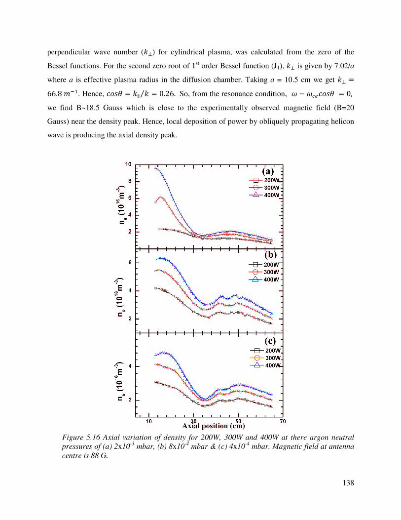
138
perpendicular wave number (K¿) for cylindrical plasma, was calculated from the zero of the
Bessel functions. For the second zero root of 1st order Bessel function (J1), K¿ is given by 7.02/a
where a is effective plasma radius in the diffusion chamber. Taking a = 10.5 cm we get K¿ =66.8 ,. Hence, = K∥ K⁄ = 0.26. So, from the resonance condition, $ − $%( = 0, we find B~18.5 Gauss which is close to the experimentally observed magnetic field (B=20
Gauss) near the density peak. Hence, local deposition of power by obliquely propagating helicon
wave is producing the axial density peak.
Figure 5.16 Axial variation of density for 200W, 300W and 400W at there argon neutral
pressures of (a) 2x10⁻³
mbar, (b) 8x10⁻⁴
mbar & (c) 4x10⁻⁴
mbar. Magnetic field at antenna
centre is 88 G.

139
Parametric studies were carried out at different pressures for different powers. Axial density is
measured at different pressures and powers and plotted in figure 5.16. Magnetic field is also
plotted in the same figure6. For, high pressure, p=4x10⁻³mbar density peak is at z=46 cm where
B is around 25G. Keeping pressure same peak decreases with power. As lower pressures, p =
8x10⁻⁴ mbar or p = 4x10⁻⁴ mbar, there are two humps in density trace, one is at B=20 G and other
being at B=40G. The higher magnetic field hump may be because of higher K¿(lower
wavelength).
5.5 Efficient Low Field Helicon Source
Helicon waves propagating near the electron cyclotron resonance cone angle boundary
can excite electrostatic fluctuations which subsequently can dump energy in the plasma. This
process is described in Section 5.2 and is shown to be responsible for peaking in density as well
as antenna plasma coupling in low field helicon discharges, where the helicon wave propagates
at a resonance cone angle with respect to the applied magnetic field. Though much of the
experiments to study the low field helicon discharges have used a uniform magnetic field,
recently Lafleur et al [9] using a diverging magnetic field near the antenna have obtained a ten
fold increase in density from the density at no magnetic field. Also reported in this work is that
using another coil (described as exhaust coil in their report), the density did not rise as much
compared to the single coil. The source coil current was varied by keeping the current in the
exhaust coil constant at one of the values between 0-5 A in 1 A steps. As for 1 A current in the
exhaust coil current, the density value must have decreased as with the case with only source
coil. Now, on top of this any current in the source coil will increase the magnetic field near the
antenna and the densities will follow the only source coil case after 1 A if the coils are taken as
identical as is the case.
When we have a magnetic field which is uniform near the antenna, as per section 5.2 the oblique
cyclotron resonance for a single mode will happen at a particular magnetic field. But in case of a
diverging magnetic field near the antenna, all the radial and axial modes in the system will have
resonance due to the availability of different magnetic fields. So it seems that magnetic field
profile near the antenna dictates the density peaking phenomena. To see the effect of magnetic
field gradient near the antenna we have used 4 different magnetic field configurations with

140
completely uniform magnetic field near the antenna to the most diverging field one can obtain
with a single coil.
Figure 5.17 shows axial variation of magnetic field when 1A current is passed for four different
magnetic field topologies used. The left most coil as shown in the experimental set up (Figure
3.2) is the first coil and the right most coil is the seventh coil. Case A corresponds to a magnetic
field profile when 1 A current is passed through 6 coils as is the case described in Section 5.3
and 5.4. Case B magnetic field is produced by taking out the first coil and keeping the other 5.
Case C magnetic field is obtained by removing the first and second coils from left and keeping
only 4 coils. Case D magnetic field corresponds to 1 A current in fourth coil by removing the
first, second, third, fifth and sixth coils.
Figure 5.17 Axial variation of magnetic field for Cases A-D when 1 A current
is passed in the coil(s).

141
Double Langmuir probe is placed at = ±18 from the antenna axial centre to measure the
ion saturation current. Both the probes have probe tips of 0.5 mm diameter tungsten wires and
are of length 3 mm. Electron temperature is measured by a RF compensated probe +18 cm away
from the antenna centre. A rogowski coil is used to measure the RF current in the antenna near
the reference leg of the antenna from which the power transfer efficiency, η = RP/ (RP + RA) is
calculated.
Figure 5.18 shows the variation of density measured at = +18 for all the cases outlined
above. As for density peaks studied so far, here also for m=+1 side the ECR peak is very small or
non-existent. Density peaked around 30 G for Case A, B and C. For the most non-uniform case
D, the density peaked ~ 50 G. As the coils are removed or field non-uniformity is increased from
Case A-case C, density at ~30 G increased but for Case D the density decreases as compared to
Case C. As the probe is kept at = +18 , for case D the magnetic field decreases rapidly and
the measured density becomes less in the diverging field region. Also on the m=+1 side, the
volume of the plasma is more than m=-1 side, so the particle loss on m=+1 side will be more.
Figure 5.18 variation of density at = +18 with applied magnetic field at
antenna centre for Cases A-D. RF power is 300W and pressure 8 X 10⁻⁴
mbar.
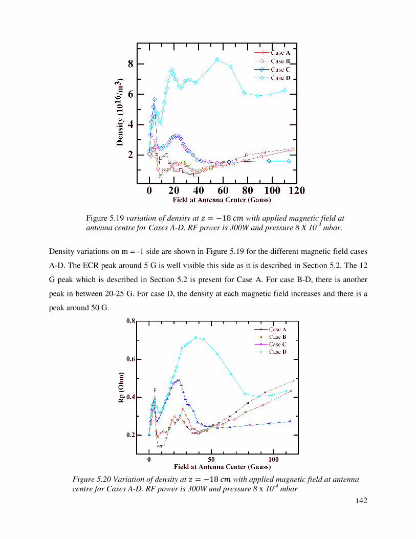
142
Density variations on m = -1 side are shown in Figure 5.19 for the different magnetic field cases
A-D. The ECR peak around 5 G is well visible this side as it is described in Section 5.2. The 12
G peak which is described in Section 5.2 is present for Case A. For case B-D, there is another
peak in between 20-25 G. For case D, the density at each magnetic field increases and there is a
peak around 50 G.
Figure 5.19 variation of density at = −18 with applied magnetic field at
antenna centre for Cases A-D. RF power is 300W and pressure 8 X 10⁻⁴
mbar.
Figure 5.20 Variation of density at = −18 with applied magnetic field at antenna
centre for Cases A-D. RF power is 300W and pressure 8 x 10⁻⁴
mbar

143
The calculated plasma resistance is shown in figure 5.20 for all the four cases. For every case the
plasma resistance has a peak ~ 5 G corresponding to the electron cyclotron resonance absorption.
For nearly uniform magnetic field cases (Case A, B and C), the plasma resistance peaked ~ 30 G.
For the single coil case D, the plasma resistance is highest and occurs ~ 50 G. As it was
discussed in Section 5.2, the plasma resistance explains the behavior on both sides of the
antenna. This behavior of density rise on both sides of antenna is different from Lafleur et al [9]
as in their case the plasma boundary on the m= -1 side is just 5 cm from the antenna and they
have measured the density in the centre of the antenna.
Figure 5.21 Increase in efficiency from the zero field case to the efficiency at the density
peak for the four field topologies shown in Figure 5.20.

144
The efficiency of the antenna is calculated using Equation 3.66. For the most uniform magnetic
field case (case A) the increase in efficiency of antenna plasma coupling from the zero field to
the peak magnetic field is nearly 21%, where as for the most non-uniform case the increase is ~
80% (Figure 5.21). As low field helicon sources are proposed recently for space propulsion [32],
using a diverging magnetic field near the antenna is well suited.
5.6 Conclusions
Multiple density peaks are observed for the first time in a helicon experiment operated at
low magnetic fields. The density peaks are shown to be observed near the resonance cone angles
of obliquely propagating helicon waves. Resonance cone propagation leading to excitation of
electrostatic fluctuations are confirmed, the amplitude of fluctuations being large at the magnetic
fields where the propagation angle coincides with the resonance cone angle. Energy transfer
from helicon waves to these fluctuations which deposit energy in the plasma is proposed to
explain the density peaks. This proposition helps in explaining the results of Wang et al where
the density peaks are observed at higher magnetic fields for higher source frequencies which is
required to satisfy the resonance condition. Measurement of density, visible light intensity and
antenna plasma resistance at low magnetic field (< 100 G) clearly shows density peaking
phenomena on both sides of the antenna at different applied magnetic fields. The density peak
observed at the electron cyclotron resonance point around 5 G, where the cyclotron frequency is
close to the source frequency of 13.56 MHz, always has higher magnitude in the “m = -1 side”,
compared to m = +1 side. This is explained by the polarization reversal of LHPW to RHPW. The
reason behind non-occurrence of 30 G peak on “m = -1 side” is not clear. The wave field
measurements have shown that || = 1 character is present near all the peaks. The antenna
dumps power on both sides simultaneously as the plasma resistance behavior can only be
explained when taking into account of the variations on both sides of the antenna. With a source
magnetic field of 88 G, density peaks are observed far away from source in the diffusion
chamber near locations close to having fields around 30 G. Phase measurements in the axial
direction show propagating and non-propagating regions. In the diffusion chamber the density
peak is explained by oblique resonance as explained in Section 5.2 by considering the measured
parallel wave number and estimated perpendicular wave number. Four different field topologies
near the antenna is used to look for effect of magnetic field gradient. It is shown that for the

145
availability of different magnetic fields near the antenna, the density on both sides along with the
antenna-plasma coupling increases which is proposed to be through a multimode oblique
resonance.

146
References
[1] Boswell, R. W. "Plasma production using a standing helicon wave." Physics Letters A 33, no. 7 (1970): 457-458.
[2] Degeling, A. W., C. O. Jung, R. W. Boswell, and A. R. Ellingboe. "Plasma production from helicon waves." Physics of Plasmas 3 (1996): 2788.
[3] Chen, F. F., X. Jiang, J. D. Evans, G. Tynan, and D. Arnush. "Low-field helicon discharges." Plasma Physics and Controlled Fusion 39, no. 5A (1997): A411.
[4] Lho, Taihyeop, Noah Hershkowitz, J. Miller, W. Steer, and Gon-Ho Kim. "Azimuthally symmetric pseudosurface and helicon wave propagation in an inductively coupled plasma at low magnetic field." Physics of Plasmas 5 (1998): 3135.
[5] Wang, S. J., J. G. Kwak, C. B. Kim, and S. K. Kim. "Observation of enhanced negative hydrogen ion production in weakly magnetized RF plasma." Physics Letters A 313, no. 4 (2003): 278-283.
[6] Sato, G., W. Oohara, and R. Hatakeyama. "Efficient plasma source providing pronounced density peaks in the range of very low magnetic fields." Applied physics letters 85, no. 18 (2004): 4007-4009.
[7] Wang, S. J., Jong-Gu Kwak, S. K. Kim, and Suwon Cho. "Experimental study on the density peaking of an RF plasma at a low magnetic field." Journal of Korean Physical Society 51 (2007): 989.
[8] Sato, G., W. Oohara, and R. Hatakeyama. "Experimental characterization of a density peak at low magnetic fields in a helicon plasma source." Plasma Sources Science and Technology 16, no. 4 (2007): 734.
[9] Lafleur, T., C. Charles, and R. W. Boswell. "Characterization of a helicon plasma source in low diverging magnetic fields." Journal of Physics D: Applied Physics 44, no. 5 (2011): 055202.
[10] Eom, G. S., Junghee Kim, and Wonho Choe. "Wave mode conversion and mode transition in very high radio frequency helicon plasma." Physics of plasmas 13 (2006): 073505.
[11] Chen, Francis F. "The low-field density peak in helicon discharges." Physics of Plasmas 10 (2003): 2586.
[12] Shamrai, Konstantin P., and Vladimir B. Taranov. "Volume and surface rf power absorption in a helicon plasma source." Plasma Sources Science and Technology 5, no. 3 (1996): 474.
[13] Cho, Suwon. "The resistance peak of helicon plasmas at low magnetic fields." Physics of
plasmas 13 (2006): 033504
[14] Blackwell, D. D., T. G. Madziwa, D. Arnush, and F. F. Chen. "Evidence for Trivelpiece-Gould modes in a helicon discharge." Physical review letters 88, no. 14 (2002): 145002-145002.
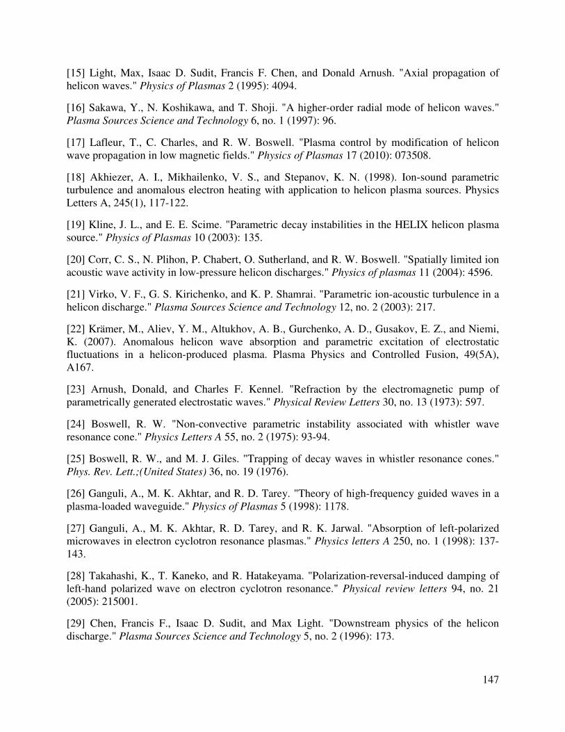
147
[15] Light, Max, Isaac D. Sudit, Francis F. Chen, and Donald Arnush. "Axial propagation of helicon waves." Physics of Plasmas 2 (1995): 4094.
[16] Sakawa, Y., N. Koshikawa, and T. Shoji. "A higher-order radial mode of helicon waves." Plasma Sources Science and Technology 6, no. 1 (1997): 96.
[17] Lafleur, T., C. Charles, and R. W. Boswell. "Plasma control by modification of helicon wave propagation in low magnetic fields." Physics of Plasmas 17 (2010): 073508.
[18] Akhiezer, A. I., Mikhailenko, V. S., and Stepanov, K. N. (1998). Ion-sound parametric turbulence and anomalous electron heating with application to helicon plasma sources. Physics Letters A, 245(1), 117-122.
[19] Kline, J. L., and E. E. Scime. "Parametric decay instabilities in the HELIX helicon plasma source." Physics of Plasmas 10 (2003): 135.
[20] Corr, C. S., N. Plihon, P. Chabert, O. Sutherland, and R. W. Boswell. "Spatially limited ion acoustic wave activity in low-pressure helicon discharges." Physics of plasmas 11 (2004): 4596.
[21] Virko, V. F., G. S. Kirichenko, and K. P. Shamrai. "Parametric ion-acoustic turbulence in a helicon discharge." Plasma Sources Science and Technology 12, no. 2 (2003): 217.
[22] Krämer, M., Aliev, Y. M., Altukhov, A. B., Gurchenko, A. D., Gusakov, E. Z., and Niemi, K. (2007). Anomalous helicon wave absorption and parametric excitation of electrostatic fluctuations in a helicon-produced plasma. Plasma Physics and Controlled Fusion, 49(5A), A167.
[23] Arnush, Donald, and Charles F. Kennel. "Refraction by the electromagnetic pump of parametrically generated electrostatic waves." Physical Review Letters 30, no. 13 (1973): 597.
[24] Boswell, R. W. "Non-convective parametric instability associated with whistler wave resonance cone." Physics Letters A 55, no. 2 (1975): 93-94.
[25] Boswell, R. W., and M. J. Giles. "Trapping of decay waves in whistler resonance cones." Phys. Rev. Lett.;(United States) 36, no. 19 (1976).
[26] Ganguli, A., M. K. Akhtar, and R. D. Tarey. "Theory of high-frequency guided waves in a plasma-loaded waveguide." Physics of Plasmas 5 (1998): 1178.
[27] Ganguli, A., M. K. Akhtar, R. D. Tarey, and R. K. Jarwal. "Absorption of left-polarized microwaves in electron cyclotron resonance plasmas." Physics letters A 250, no. 1 (1998): 137-143.
[28] Takahashi, K., T. Kaneko, and R. Hatakeyama. "Polarization-reversal-induced damping of left-hand polarized wave on electron cyclotron resonance." Physical review letters 94, no. 21 (2005): 215001.
[29] Chen, Francis F., Isaac D. Sudit, and Max Light. "Downstream physics of the helicon discharge." Plasma Sources Science and Technology 5, no. 2 (1996): 173.
148
[30] Tysk, Shane M., C. Mark Denning, John E. Scharer, and Kamran Akhtar. "Optical, wave measurements, and modeling of helicon plasmas for a wide range of magnetic fields." Physics of
Plasmas 11 (2004): 878.
[31] Sudit, Isaac D., and Francis F. Chen. "Discharge equilibrium of a helicon plasma." Plasma
Sources Science and Technology 5. (1996): 43.
[32] Chen, Francis F. "Permanent magnet helicon source for ion propulsion." Plasma Science,
IEEE Transactions on 36, no. 5 (2008): 2095-2110.

149
Chapter 6
Current Free Double Layer
6.1 Introduction
Monotonic potentials form in the boundary of a plasma vessel or any material inserted in
plasma and these potential structures are known as sheaths. Double layers (DL) or double
sheaths are potentials formed in the bulk of the plasma. Normally DLs are formed in the
interface of two different plasmas and need a current to maintain this potential. Current free
double layers are potential structures formed self consistently in a current less plasma. Recently
many experiments reported observations of DLs in current-less systems. Most of the works on
current free double layer (CFDL) are reported in low pressure geometrically expanding helicon
plasma systems with a diverging magnetic field. Still many experiments are going on to find out
the formation mechanism of CFDLs as well as to find out the role of different external
parameters like neutral pressure [1], antenna frequency [2], magnetic field [1, 3-4] as well as the
strength and location of magnetic field gradient [5-8]. Electric fields can be created in the bulk of
geometrically expanding plasmas with or without diverging magnetic fields either by the normal
Boltzmann plasma expansion [8-10] or by DL like self consistent potential structures [1-8].
Ambipolar plasma expansion and subsequent potential formation is discussed in Section 6.2
followed by an introduction to double layers in Section 6.3. A DL normally needs finite relative
ion-electron drifts or a current to be sustained [39]. Current free plasmas can also sustain
potential structures in an expanding geometry. These CFDLs are explained in Section 6.4 along
with recent experimental and conceptual developments in CFDLs produced in low pressure
helicon discharges. One of the common features of helicon CFDL experiments is a dielectric
source tube around which a helical antenna is wrapped to produce plasma. It is believed that
finite amount of charging of this dielectric wall is necessary to form a CFDL [37-38]. In RF
discharges a floating object can acquire a negative potential known as the DC-self bias. In this

150
thesis work a borosilicate glass source tube is used and its charging dependence on various
external parameters like RF power, gas mass, gas pressure and magnetic field is studied and the
results are described in Section 6.5. Role of magnetic field gradient and the location of maximum
field gradient are studied in a low pressure and low power RF plasma and the results are
presented in Section 6.6.
6.2 Boltzmann Plasma Expansion
For Maxwellian electrons in a plasma, electron temperature, density and plasma potential
are related. Plasma density decreases when relatively denser plasma expands from the source
region of a discharge to a vacuum chamber with area larger than the source. This density
decreases creates a potential fall away from the source.
Consider a plasma source where density near source as ; and plasma potential ó = 0 and take
two points A and B away from the source. The potential and temperature are respectively óS and î(S at location A. Density lS for a Maxwellian plasma electrons at A can be expressed as
k = uà(−ò/Ù) (6. 88 )
Similarly for a location B, if the potential and temperature are respectively ó and î( then
density l for a Maxwellian plasma electrons there can be expressed as
TU = uà(−VU/ÛuU) (6. 89 )
From the above two equations we can have
2 Dkk3E = ò3Ù3 − òÙ (6. 90 )
So if the temperature at location A and B are equal with î(S = î( = î( then the potential
difference ó − óS = ∇ó between location B and A can be written as
ÌV = −Ûu DTXTUE (6. 91 )

151
So if lS > l i.e. if the density drops from location A to location B then a potential drop will
be created as per Equation 6.4.
When a plasma expands in a diverging magnetic field, the magnetized electrons will follow the
field lines and flow in a larger area. When the magnetic field strength decreases, the flux tube
area increases. If the magnetic flux tube area and field strength at o = 0 are ;, 9; and at x
are ?, 9? [Figure 6.1] then
XU = XU (6. 92 )
As the magnetic field diverges, the plasma density decreases and the density ; at o = 0 is
related to density at o by
= U
U = XX (6. 93 )
Figure 6.1 Ambipolar plasma expansion in diverging magnetic field [12].
152
Assuming ions entering the location o = 0 at Bohm velocity , the ion continuity equation will
be
(i)(i)(i) = 3 (6. 94 )
, where (o) is the velocity at o. The ion velocity can be found from the energy conservation
equation as
(i) = 3 + [ò(i) (6. 95 )
Thus when the plasma expands, density decreases and a potential ó(o) is set up which
accelerates the ions. This kind of ambipolar plasma expansion with or without a diverging
magnetic field is reported by many authors in RF discharges. Lafleur et al [8] have reported ion
acceleration over a length of 15 cm with ion beam energy of 18 eV in an expanding low pressure
(~ 4.3 × 10 mbar, Argon) helicon plasma source at low magnetic fields of ~ 20 G using a
retarding field energy analyzer (RFEA). Corr et al [9] have observed ion beams with energy ~ 50
eV in a geometrically expanding capacitive discharge. Longmier et al [10] have observed
ambipolar ion acceleration over a length of 104-105 Debye lengths with ion speeds four times ion
sound speed at 30 kW RF power and 1.7 kG magnetic field in low argon pressures of ~2.6 ×10 9 mbar.
6.3 Double Layer
A double layer (DL) in its simplest form is a sandwich of two oppositely charged space
charge layers. It is different from the normal sheath as the DL forms in the bulk of the plasma
where as the former forms on boundary of any material inserted into the plasma or on the
boundary of the vessel containing the plasma. A typical potential, electric field and space charge
density profile of DL in a plasma is given in Figure 6.2. Though the total charge of the DL is
zero, quasi-neutrality is violated inside the DL. A DL can have extended pre-sheaths on both
sides much like a sheath to match the conditions of the quasi-neutral plasma on either side.

The potential drop inside the DL can be as large as 2000 times [14
(in Volts) to an order of electron temperature [16] with the for
the latter as the weak DLs. There are DLs which can have drops even less than electron
temperature which are known as the ion acoustic type DLs (IADL).
Figure 6.2
charge distribution in
The potential drop inside the DL can be as large as 2000 times [14-15] the electron temperature
(in Volts) to an order of electron temperature [16] with the former known as the strong DLs and
the latter as the weak DLs. There are DLs which can have drops even less than electron
temperature which are known as the ion acoustic type DLs (IADL). Chan et al.
Electric potential, electric field and space
charge distribution inside a double layer [13].
153
15] the electron temperature
mer known as the strong DLs and
the latter as the weak DLs. There are DLs which can have drops even less than electron
Chan et al. [16] reported the
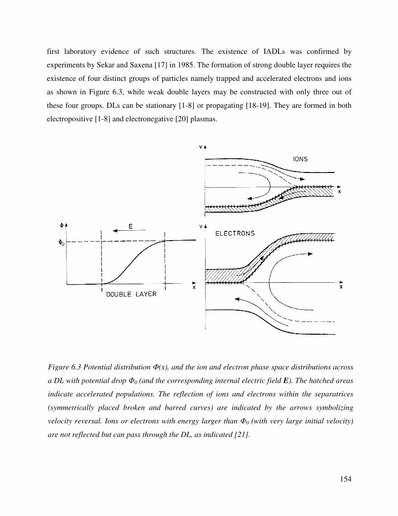
154
first laboratory evidence of such structures. The existence of IADLs was confirmed by
experiments by Sekar and Saxena [17] in 1985. The formation of strong double layer requires the
existence of four distinct groups of particles namely trapped and accelerated electrons and ions
as shown in Figure 6.3, while weak double layers may be constructed with only three out of
these four groups. DLs can be stationary [1-8] or propagating [18-19]. They are formed in both
electropositive [1-8] and electronegative [20] plasmas.
Figure 6.3 Potential distribution Φ(x), and the ion and electron phase space distributions across
a DL with potential drop Φ0 (and the corresponding internal electric field E). The hatched areas
indicate accelerated populations. The reflection of ions and electrons within the separatrices
(symmetrically placed broken and barred curves) are indicated by the arrows symbolizing
velocity reversal. Ions or electrons with energy larger than Φ0 (with very large initial velocity)
are not reflected but can pass through the DL, as indicated [21].

155
Electric fields inside the plasma are often interesting as they can be used as source of thrust for
space propulsion [22-23] and also accelerated ions can be used to functionalize materials [24] of
interest to semiconductor industry. As a source for charged particle acceleration, they are
believed to explain some important astrophysical phenomena like aurora formation [25]. Alfven
[25], suggested that a DL present in the magnetosphere can accelerate electrons to earth’s upper
atmosphere which leads to the precipitation and the subsequent observation of aurora. With
rocket-borne detectors McIlwain [26], found the presence of mono energetic electrons which
suggested electrostatic acceleration. Later Satellite observations by Forrest Mozer [27] in the
magnetosphere have revealed electrostatic shocks aligned to magnetic field. It is recently
proposed that double layers may play a significant role in supplying and accelerating plasma in
magnetic coronal funnels [28].
6.4 Current Free Double layer
Perkins and Sun [29] analytically suggested that current free plasmas can sustain a
potential drop in a diverging magnetic field by solving the Vlasov equation. Hatakeyama et al.
[30] observed the first experimental CFDL by mixing two plasmas of unequal electron
temperature in a triple plasma device. Hairapetian and Stenzel [31] created two-electron
temperature plasma and then allowed its expansion. Adjusting the individual temperatures of the
two groups of electrons they have observed CFDL formation.
6.4.1 Helicon CFDL experiments
Charles and Boswell [11] observed the first helicon CFDL in which they have measured a
sharp potential drop of 45 V in ~ 50 Q> along the magnetic field. The experiment was performed
at 250 W RF power and a pressure of 0.4 mTorr with 130 G magnetic field in the source
chamber which decreased to few tens of Gauss in the diffusion chamber. The experimental set
up, the axial potential profile and axial density profile are shown in Figure 6.4. Argon and
Hydrogen plasmas were used for CFDL formation and ion beams accelerated in the CFDL are
observed in the downstream by a retarding field energy analyzer [32]. The formation of double
layers in current-free plasmas and associated ion beams were confirmed by similar experiments
[1-5, 7, 33-35].

156
Charles and Boswell [36] also did the time evolution study of the CFDL formation and found
that the current-free double layer was formed in the first 100 µs of the discharge. Charles [37]
also showed that CFDL formation was accompanied by negative charging of the source walls.
Meige et al [38] in 1D PIC simulations have shown that finite amount of source wall charging is
necessary for CFDL formation.
6.4.2 Helicon CFDL Models
After the observation of CFDL in helicon plasmas, many models have tried to explain the
observations of CFDL formation in low pressure helicon discharges by taking various groups of
Figure 6.4 Chi-Kung source, axial applied magnetic field, measured axial plasma
potential and density at 250 W RF power, 0.2 mTorr and 130 G at source [11].

157
trapped and free electron distributions. A current driven DL is modelled using four groups of
particles as free and trapped electron and ions [39].
Taking a Maxwellian upstream electron population, with no additional energetic electron
population Chen [40] considered a Boltzmann plasma expansion in the diverging magnetic field.
As the plasma expands in a diverging magnetic field, the density and plasma potential fall
according to Boltzmann expansion. For a potential drop of 0.5 Kî(/<, the ions get accelerated
and attain the Bohm velocity after which their density decrease is slower than that of electrons.
So the plasma expansion is considered to be a simple Boltzmann expansion until the point where
quasi-neutrality breaks down (n = n0 e -1/2) and the double layer forms. The double layer potential
is self-consistently set such that equal electron and ion fluxes can flow across it, and it is
therefore current free. As to a floating material inside plasma the ion and electron fluxes are
equal, this double layer structure thus evolved is current free in nature. For Argon plasma a
CFDL drop of ~ 5.2 kTe/e was proposed. This model does not take into account the collisions and
also cannot explain the 165 eV ion beams observed by Weibold et al [35] for a 14 eV plasma.
Lieberman et al [41] in a diffusive model used a group of fast electrons being accelerated
by the CFDL towards upstream plasma along with the four group of particles needed for a
current driven DL. These fast electrons will get reflected from the source end wall sheath to
ensure that the DL formed is current free. As the source diameter is less than the diffusion
chamber diameter in all the CFDL experiments, the loss of electrons in the upstream will be
higher upstream. This electron loss is compensated by the extra accelerated group of particle
travelling towards the source from the diffusion by increasing the ionization in the source region.
Their explanations can explain the pressure dependency of CFDL strength observed in the
experiments. For very low neutral pressure where collisions are sparse, additional ionization in
the source cannot happen and the CFDL vanishes and for higher pressures there is no longer a
need for ionization by the energetic electrons and the double layer vanishes. But so far in
experiments these fast electrons are not observed though there is experimental evidence that the
source ionization increases [2] with CFDL formation.
Ahedo et al [42] used a Bi-Maxwellian electron distribution and shown that for
collisionless plasma, the ratio of hot electron density and temperature to Maxwellian electron
density and temperature plays a role in CFDL formation.
158
Takahashi et al [43] measured the electron energy distribution in an expanding low
pressure helicon discharge. In the upstream they found a Bi-Maxwellian distribution with free
and trapped electrons. The break energy of the distribution upstream was found to be the CFDL
potential drop so that the hotter population escapes the source. The temperature of the trapped
electron was higher than the free electrons as the trapped electron stay for longer time being
trapped in the wall sheath and the CFDL potential. The fast electrons stay considerably for a
lesser time in the source. The faster electrons which go to the right side grounded wall sheath get
reflected and then again get accelerated when they enter the upstream. So a single source of Bi-
Maxwellian electrons can sustain the CFDL. In the downstream they have observed only the
hotter population which has escaped from the source.
6.4.3 Helicon CFDL instabilities
Observation of two different types of low frequency instabilities are reported in helicon
CFDL experiments. Aanesland et al [1] have observed an instability in the frequency range of
10-20 kHz concurrent with the CFDL in a low pressure helicon discharge. Electrons accelerated
from the downstream plasma through CFDL were believed to excite an ionization instability in
the upstream plasma. They have done a theoretical calculation for excitation of ionization
instability by an electron beam in the low pressure upstream plasma and found the dispersion of
the ionization instability and its growth rate. The theoretically calculated pressure dependency of
the ionization instability frequency matched quite well with the experimental data.
Thakur et al [2] reported observation of ion acoustic instability of 17.5 kHz, that is
excited when the source frequency is below 12 MHz. For frequencies between 12-15 MHz stable
CFDL formations was reported along with increase in signal-to-noise ratio in all electrostatic
probes, upstream plasma density and velocity of ions downstream. For low RF frequencies the
coupling to plasma is shown for their system to be better, so that a strong CFDL tries to form but
that results in formation of high energy beams through acceleration in the high potential drop
which were proposed to drive the ion acoustic velocity. They proposed that this electrostatic
instability will self limit the formation of strong CFDL formation.
The above mentioned results are different from each other as in case of Aanesland et al [1] the
instability is concurrent with the CFDL where as for Thakur et al [2] the CFDL formed only after
the ion acoustic instability got suppressed at higher source frequencies.

159
6.4.4 Effect of Magnetic field Strength and Gradient
Charles and Boswell [3] studied the role of magnetic field on CFDL formation. By
increasing the magnetic field they have observed ion beam formation in downstream plasma for
a critical magnetic field of 50 G in the source. The source potential and density increased
simultaneously at 50 G but in the downstream plasma the effect was little. Ion magnetization at
50 G is attributed to this transition from an expanding plasma to a plasma containing a CFDL.
When the ion is magnetized the ion loss to the radial wall decreases and amounted to the density
rise. Similar results were obtained by Takahashi et al [4] in EMPI source have shown that for
two different dielectric source tubes of radii of 3.25 cm and 2.3 cm, the CFDL is formed for
125 G and 195 G respectively the values of these magnetic fields also are the magnetic fields
where the ions got magnetized.
Though the observation of the CFDL were reported by many authors, the location of the
CFDL with respect to the geometrical expansion point and also with respect to the maximum
magnetic field gradient location was not clear. The role of magnetic field gradient and its
location was studied by Sutherland et al [7], Byhring et al [5] and Schroder et al [6]. Sutherland
et al. [7] showed that the double-layer strength could be scaled by a factor of at least 2 in a
bigger system and that the double layer presumably forms in the vicinity of maximal gradient of
the magnetic field. Byhring et al [5] changed the magnetic field gradient by using an extra coil in
which the current is passed in the same direction as the other coils. So by increasing the current
in their last coil they could decrease the magnetic field gradient which location was much inside
the source plasma. They have found that CFDL only formed for up to 8 A in the last coil which
was confirmed by RFEA measurements. For their case CFDL formed 6 cm downstream of the
geometrical expansion location. A study on independent effects of geometric expansion,
magnetic field and field gradient along with its location are studied by Schroder et al [6] in
VINETA device. For magnetic field gradient location coinciding with the geometric expansion
they have found the CFDL strength is highest. For low magnetic fields the CFDL formed nearer
to the diameter change location but for higher magnetic field the DL was pushed to the
downstream plasma. They have also reported that for the geometric expansion location nearer to
the source stronger potential drops are formed.
160
6.5 Study of Dielectric Wall Charging
Current free double layers (CFDL) are observed [11] in diverging magnetic field low
pressure helicon experiments with an RF antenna wrapped around a cylindrical source tube made
of dielectric material and it is believed [37-38] that dielectric glass wall charging lifts the plasma
potential in the source chamber of this kind of discharges. Meige et al [38] have done 1D
simulation and found that finite wall charging is necessary for the CFDL formation and it may be
noted that this can be a reason that no CFDL formation is reported so far without use of dielectric
source tubes. The plasma potential of the source region of helicon CFDL experiment depends on
the loss rate of electrons and ions whereas the flux of ions to the dielectric wall determines the
wall potential.
When a material body is inserted inside an electron-ion plasma, the floating body is
negatively charged by the electrons. This negative potential is known as the floating potential
(ó ) of the material and it accelerates the less mobile ions near the wall so that the total current to
the floating object is zero. This floating potential depends on electron temperature and electron
to ion mass ratio and is expressed as ó = (Kî( 2<⁄ )³ln(2 ê⁄ )´, where K, î(, and ê are the
Boltzmann’s constant, electron temperature, electron mass and ion mass respectively. As
Mm << , fV is always negative with respect to the plasma potential.
When a high frequency electric field is applied to a floating dielectric which is exposed to
the plasma, the plasma electrons respond quickly compared to the heavier ions. This creates an
imbalance in the currents flowing to the dielectric body and the electrons have to charge the body
to a negative potential such that the heavier ions are accelerated resulting in a flux balance of
electrons and ions. Emeleus and Garscadden [44] have shown this DC voltage generation as
process of rectification by a non-linear sheath in response to harmonic oscillation of RF voltage.
Butler and Kino [45] have given a detailed theory of this sheath rectification process for an
antenna outside a glass vessel which acts as a capacitance along with measurement of the DC
bias voltage inside a glass wall surface exposed to the plasma. This potential is sum of the
floating potential of a DC plasma system as described earlier and another additional potential
because of difference in response of electrons and ions to the high frequency oscillating electric
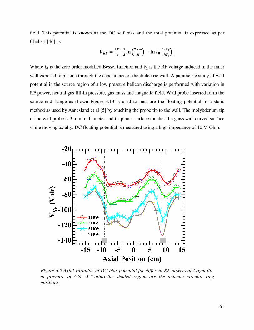
161
field. This potential is known as the DC self bias and the total potential is expressed as per
Chabert [46] as
òì = CÙ DÇ E − | DòCÙE
Where í; is the zero order modified Bessel function and ó, is the RF volatge induced in the inner
wall exposed to plasma through the capacitance of the dielectric wall. A parametric study of wall
potential in the source region of a low pressure helicon discharge is performed with variation in
RF power, neutral gas fill-in pressure, gas mass and magnetic field. Wall probe inserted form the
source end flange as shown Figure 3.13 is used to measure the floating potential in a static
method as used by Aanesland et al [5] by touching the probe tip to the wall. The molybdenum tip
of the wall probe is 3 mm in diameter and its planar surface touches the glass wall curved surface
while moving axially. DC floating potential is measured using a high impedance of 10 M Ohm.
Figure 6.5 Axial variation of DC bias potential for different RF powers at Argon fill-
in pressure of 4 × 10 !"#.the shaded region are the antenna circular ring
positions.

162
Figure 6.5 shows the variation of DC bias voltage with RF power at 200 G and 4 × 10
mbar of Argon neutral pressure. The axial locations close to the antenna straps have higher wall
potential and near the ring connected to the live side of the matching network wall charging is
high, the behaviour being more pronounced for higher RF powers. Figure 6.6 shows the variation
of wall potential at z = +9 cm (near the antenna ring) with RF power at 4 × 10 mbar. As
increasing the RF power increases the RF voltage on the antenna, according to Equation 1, the
DC bias increases.
To see the effect of neutral gas pressure in detail, DC bias is measured near both the
antenna rings at z = +9 cm and z = -9 cm for different pressure at 300 W RF power and is shown
in Figure 6.7. The DC bias increases as the pressure is decreased from 4 x 10⁻³ mbar at a
magnetic field of 200 G and for pressures less than 6 x 10⁻⁴ mbar it again starts to decrease. It
Figure 6.6 Variation of DC bias potential with power near antenna ring at z = +9 cm at
Argon pressure of 4 × 10 !"#.
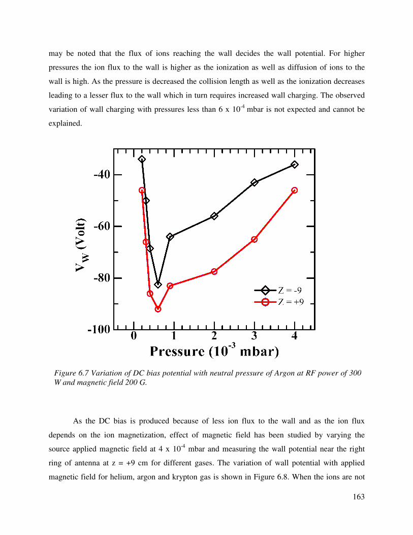
163
may be noted that the flux of ions reaching the wall decides the wall potential. For higher
pressures the ion flux to the wall is higher as the ionization as well as diffusion of ions to the
wall is high. As the pressure is decreased the collision length as well as the ionization decreases
leading to a lesser flux to the wall which in turn requires increased wall charging. The observed
variation of wall charging with pressures less than 6 x 10⁻⁴ mbar is not expected and cannot be
explained.
As the DC bias is produced because of less ion flux to the wall and as the ion flux
depends on the ion magnetization, effect of magnetic field has been studied by varying the
source applied magnetic field at 4 x 10⁻⁴ mbar and measuring the wall potential near the right
ring of antenna at z = +9 cm for different gases. The variation of wall potential with applied
magnetic field for helium, argon and krypton gas is shown in Figure 6.8. When the ions are not
Figure 6.7 Variation of DC bias potential with neutral pressure of Argon at RF power of 300
W and magnetic field 200 G.
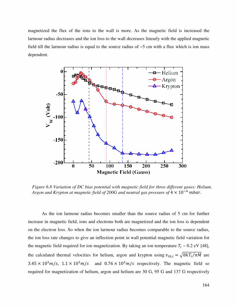
164
magnetized the flux of the ions to the wall is more. As the magnetic field is increased the
larmour radius decreases and the ion loss to the wall decreases linearly with the applied magnetic
field till the larmour radius is equal to the source radius of ~5 cm with a flux which is ion mass
dependent.
As the ion larmour radius becomes smaller than the source radius of 5 cm for further
increase in magnetic field, ions and electrons both are magnetized and the ion loss is dependent
on the electron loss. So when the ion larmour radius becomes comparable to the source radius,
the ion loss rate changes to give an inflection point in wall potential magnetic field variation for
the magnetic field required for ion magnetization. By taking an ion temperature î& ~ 0.2 eV [48],
the calculated thermal velocities for helium, argon and krypton using IAJ,& = 8Kî& ê⁄ are
3.45 × 10./, 1.1 × 10./ and 0.76 × 10./ respectively. The magnetic field so
required for magnetization of helium, argon and helium are 30 G, 95 G and 137 G respectively
Figure 6.8 Variation of DC bias potential with magnetic field for three different gases: Helium,
Argon and Krypton at magnetic field of 200G and neutral gas pressure of 4 × 10 !"#.

165
compared to magnetic fields at the respective inflection points of 42 G, 91 G and 135 G in Figure
6.8.
6.6 Experimental Observations of multiple CFDL
In current driven double layers (CDDL) the potential structure is obtained by forcing two
plasmas with different properties like plasma potential, temperature or velocity distribution to
mix. They need an external current to sustain the electric field in the DL. Anode double layer
(ADL) is a CDDL in collisional plasma (high neutral pressure) where potential structure forms
on a positively biased electrode in contact with plasma. So the ADL is formed between the
newly formed plasma (with high plasma potential) around or near the electrode and the pre-
existing plasma (lower plasma potential). The potential drop is nearly the ionization potential of
the gas used. In the presence of an ADL if the potential of the anode is increased, multiple
double layers are reported.
Stronger potential drops in CFDLs are proposed to be limited by beam driven instabilities [2].
Increasing source magnetic field, the CFDL strength was shown to saturate for higher magnetic
fields when ions are magnetized [3-4]. Decreasing the neutral pressure though the strength of DL
Figure 6.9 Experimental set up with new coil positions to study the role of magnetic field
gradient on CFDL formation.

166
increases, the DL vanishes for very low pressures [1]. As a CFDL is fundamentally current-less,
parameters important to increasing the source plasma potential in a controlled manner without
disturbing the plasma matching conditions are unknown. Instability free strong and stable
CFDLs are need of space plasma thrusters employing helicon sources.
Figure 6.9 Axial component of dc magnetic field and (c) its gradient for different coil
current. 4 coils are placed at -24.5 cm, -6.5 cm, 12.5 cm, and 28 cm with +95 A. 5th
coil is
placed at 46 cm and given currents are +35 A, 0 A, -35 A, and -95 A.

167
A new magnetic field configuration is used to study the role of magnetic field gradient on CFDL
formation and structure. Five coils located at z = -24.5 cm, -6.5cm , 12.5 cm, 28 cm, and 46 cm,
are used to produce axial magnetic field in source and expansion chambers (Figure 6.9). While a
single power supply is used to power Coils I-IV in series, an independent power supply feeds the
current Iv to the Coil V. Thus by keeping current Ii-Iiv in coils I-IV fixed, the current Iv can be
varied to achieve different gradients near the interface and the field configuration in expansion
chamber. Plots of axial magnetic field and Magnetic field gradient for a fixed current of +95A in
Coils I-IV and different values of Iv (from 0 A to -95A; negative sign implying a current
direction opposite to that in Coils I-IV), are shown in Figure 6.10.
Plasma is produced with Argon gas introduced in the expansion chamber using a mass flow
controller and pressure is maintained at ~ 2 x 10⁻⁴ mbar. RF power of 100 W is applied to the
Helicon antenna with reflected power <2%. With Iv = 0A, plasma potential variation with
magnetic field produced by only four coils is shown in Figure 6.11. For magnetic field ~ 90 Gin
the source chamber, a jump in plasma potential is evident and for magnetic field values more
than 90 G, the change in plasma potential is very less. Charles and Boswell [3] have already
Figure 6.11 Plasma potential variation on axis measured at z=18 cm with
source magnetic field for 100 W RF power and 2x10⁻⁴
mbar Argon pressure.

168
shown that the source plasma potential increases for a magnetic field value at which the ions are
magnetized. With an ion temperature of 0.2 eV [48], the experimental value is quiet close to the
calculated value for an ion to magnetize in a ~ 5cm plasma radius source.
To see the effect of magnetic field gradient plasma potentials are measured using an
emissive probe, as a function of Iv at z= 18 cm (inside the source) at the axis and are shown in
Figure 6.12. It is seen that the plasma potential, on the axis, increases initially as Iv is changed
from 0 to Iv = -35 A. Further change of Iv results in decrease of this potential till Iv= -50 A.
Finally, for larger negative values of Iv, plasma potential starts increasing again and continues
rising and saturates near Iv = -95 A. It may be noted that the magnetic field in the source region
does not change significantly as Iv is changed from0A to -95A. The gradient at the interface,
however, changes from 4.7 Gauss/cm to 11 Gauss/cm.
Figure 6.10 Variation of floating potential near the wall and plasma potential at the axis
measured at z=20 cm in the source chamber with the last coil negative current. Current in
four other coils are 95 A each. RF power 100 W, pressure 2x10⁻⁴
mbar.
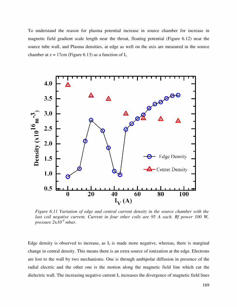
169
To understand the reason for plasma potential increase in source chamber for increase in
magnetic field gradient scale length near the throat, floating potential (Figure 6.12) near the
source tube wall, and Plasma densities, at edge as well on the axis are measured in the source
chamber at z = 17cm (Figure 6.13) as a function of Iv.
Edge density is observed to increase, as Iv is made more negative, whereas, there is marginal
change in central density. This means there is an extra source of ionization at the edge. Electrons
are lost to the wall by two mechanisms. One is through ambipolar diffusion in presence of the
radial electric and the other one is the motion along the magnetic field line which cut the
dielectric wall. The increasing negative current Iv increases the divergence of magnetic field lines
Figure 6.11 Variation of edge and central current density in the source chamber with the
last coil negative current. Current in four other coils are 95 A each. Rf power 100 W,
pressure 2x10⁻⁴
mbar.

170
at the interface and more field lines pass through the wall of the insulated source chamber. This
will lead to trapping of the magnetized electrons reaching the dielectric wall, as proposed by
Takahashi et al. [49].The electrons bounce back and forth between the field lines cutting the
source tube wall on one side and the sheath on the insulated end plate of the source chamber on
the other side. This back and forth motion of electrons, causes additional local ionization. The
area of the shell of the terminated field lines not going to expansion chamber increases as Iv
becomes more negative. As edge density increases/decreases wall charging should
decreases/increases. This should lead to lower/higher floating potential near the wall. This is
evident from the floating potential measurement near the source chamber wall (Figure 6.12). As
the edge density increases floating potential decreases. Additional ionization near the edge leads
to reduction in the radial loss of ions and hence electrons from the bulk plasma. Now to maintain
electron energy balance, the plasma potential in the source has to increase to facilitate more axial
electron loss and thus compensate less electron loss in the radial direction. The decrease of this
plasma potential between Iv = -35A and -50A is a new feature which may be due to very strong
divergence of field lines near the interface. In addition to strong gradients and divergence, as
discussed below, an axial null and a radial cusp gets formed for negative values of Iv. The
positions of the null and cusp are within the expansion chamber for Iv≳ -50A. The increase in the
potential, for Iv≳ -50A may be the effect of presence of the null and the cusp in expansion
chamber.
Further studies were made by scanning plasma potential axially for different Iv. Figure 6.14
shows the axial plasma potential variation for 95A current in the first four coils and Iv = +35 A,
0A, -35A and -95A. For Iv = +35 A, the plasma potential is constant from z=15-20 cm and falls
smoothly, from ~ 100V to ~ 50V over a distance of ~ 8 cm remaining constant at 50V beyond
z=28 cm and thus indicating the presence of a broad CFDL. Upstream plasma density and
temperature are ~ 3x1016 cm-3 and ~ 6 eV respectively. This corresponds to a Debye length (λD)
of 0.1 mm and therefore a CFDL with potential drop of ~ 8 kTe/e and width ~800 λD is formed.
For Iv = 0A, the plasma potential structure evolves to a narrower DL structure. A constant
potential of 150V up to z=20cm, is followed by a sharp fall to 100V, within ~ 4 cm and a further
slower fall to ~50V at z= 34cm, beyond which the potential remains constant at 50V. Upstream
density and temperature at the axis remains same. The potential in the region of z=20-34 cm,

171
thus, exhibits a knee like structure, with total drop of 100V, the drop in within first 4 cm
(~400λD) being ~50V.
As Iv is changed further to -35A, the potential in the region z=15-20 cm rises to 156V and drops
within ~ 4 cm to 100V followed by a slower drop to 54V from z=24 cm to z= 34 cm, beyond
which it becomes constant at ~ 54V. The knee like feature seen in case of Iv = 0A becomes more
prominent in this case with an initial drop of ~ 56V in ~ 4cm (~400λD) followed by further fall
of ~46V over ~10 cm.
Finally, as Iv is changed to -95A, instead of the knee like structure seen in above two cases, a
multiple DL structure is seen. The potential between z=15-20 cm now goes up to 300V and this
Figure 6.12 Variation of plasma potential along the axis of the device for different
current in the last coil; circle -95 Amp, square -35 Amp, Triangle 0 Amp and star =35
Amp. Current in other four coils placed at 30.5 cm, 18 cm, 10.6 cm, 3cm are +95 Amps
each.
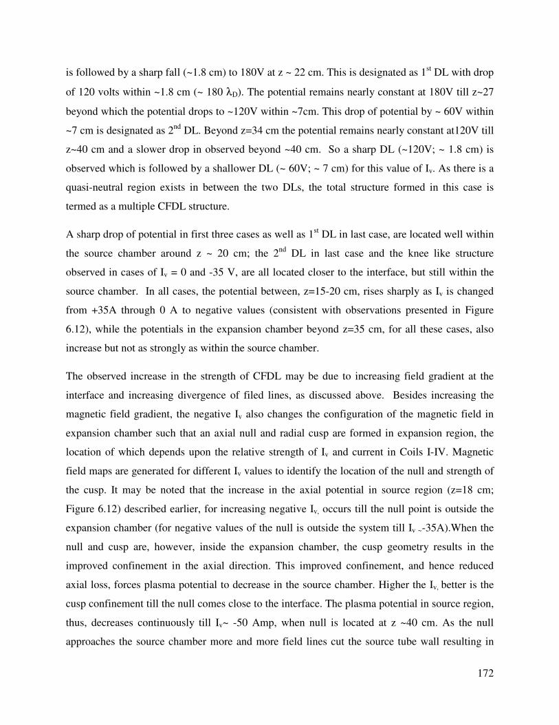
172
is followed by a sharp fall (~1.8 cm) to 180V at z ~ 22 cm. This is designated as 1st DL with drop
of 120 volts within ~1.8 cm (~ 180 λD). The potential remains nearly constant at 180V till z~27
beyond which the potential drops to ~120V within ~7cm. This drop of potential by ~ 60V within
~7 cm is designated as 2nd DL. Beyond z=34 cm the potential remains nearly constant at120V till
z~40 cm and a slower drop in observed beyond ~40 cm. So a sharp DL (~120V; ~ 1.8 cm) is
observed which is followed by a shallower DL (~ 60V; ~ 7 cm) for this value of Iv. As there is a
quasi-neutral region exists in between the two DLs, the total structure formed in this case is
termed as a multiple CFDL structure.
A sharp drop of potential in first three cases as well as 1st DL in last case, are located well within
the source chamber around z ~ 20 cm; the 2nd DL in last case and the knee like structure
observed in cases of Iv = 0 and -35 V, are all located closer to the interface, but still within the
source chamber. In all cases, the potential between, z=15-20 cm, rises sharply as Iv is changed
from +35A through 0 A to negative values (consistent with observations presented in Figure
6.12), while the potentials in the expansion chamber beyond z=35 cm, for all these cases, also
increase but not as strongly as within the source chamber.
The observed increase in the strength of CFDL may be due to increasing field gradient at the
interface and increasing divergence of filed lines, as discussed above. Besides increasing the
magnetic field gradient, the negative Iv also changes the configuration of the magnetic field in
expansion chamber such that an axial null and radial cusp are formed in expansion region, the
location of which depends upon the relative strength of Iv and current in Coils I-IV. Magnetic
field maps are generated for different Iv values to identify the location of the null and strength of
the cusp. It may be noted that the increase in the axial potential in source region (z=18 cm;
Figure 6.12) described earlier, for increasing negative Iv, occurs till the null point is outside the
expansion chamber (for negative values of the null is outside the system till Iv ~-35A).When the
null and cusp are, however, inside the expansion chamber, the cusp geometry results in the
improved confinement in the axial direction. This improved confinement, and hence reduced
axial loss, forces plasma potential to decrease in the source chamber. Higher the Iv, better is the
cusp confinement till the null comes close to the interface. The plasma potential in source region,
thus, decreases continuously till Iv~ -50 Amp, when null is located at z ~40 cm. As the null
approaches the source chamber more and more field lines cut the source tube wall resulting in

173
increased particle loss along the field lines to the source chamber wall. This leads to more
electrons to bouncing back and forth between the end wall sheath and sheath near the inner wall
of the source following the magnetic field lines which intersect the source tube wall, leading to
higher edge density as observed. So there are two processes involved. One is reduced loss in
axial direction due to the magnetic cusp and the other is reduced loss in the perpendicular
direction because of increase in number of lines intersecting the source wall, which subsequently
leads to edge ionization. Under this situation the plasma potential in the source chamber has to
go up to increase the loss and maintain electron energy balance. Thus stronger DL is observed as
the null moves closure to interface and in the process the cusp becomes stronger.
The saturation in the source plasma potential with Iv can be understood looking at the radial
plasma potential profile shown in Figure 6.15, measured at z=18 cm using an L-shaped emissive
probe. With the increase in source plasma potential, the radial electric field increases and
enhances the radial loss of ions to the wall, so that the process of increasing the plasma potential
by increasing magnetic field gradient is limited. The loss of more ions for higher values of Iv is
Figure 6.15 Radial variation of plasma potential with Iv measured at z=18 cm with
an L-shaped emissive probe for 100W RF power and 2x10⁻⁴
mbar Argon pressure.

174
also evident from the measured lower values of wall potential (Figure 6.12) and higher values of
edge density (Figure 6.13).
Diverging field with strong magnetic field gradient at the interface, results in the formation of
strong CFDL (50-100V corresponding to 8-16 kTe/e with widths ~180-400λD) in source region.
Change of Iv from positive values through 0A to negative values increases the strength of CFDL
and at Iv = -95A, a multiple CFDL is formed, with 2nd DL located in source chamber close to the
interface in the region of strong field gradient. For negative Iv values, an axial null and an
asymmetric radial cusp is formed which move closer to the interface with the cusp becoming
stronger for larger values of negative Iv. The change of trapped and free particle populations in
source and expansion chamber, due to the presence of the null and the cusp, may be responsible
for the observed features. Even though the exact role of null and cusp geometry near the
interface is not clear, it is clear from the experimental observation that it is possible to have a
control on the strength of the DL by changing magnetic field gradient.
6.7 Summary of Chapter 6
Double layers and Current free double layers are discussed with emphasis on helicon
CFDLs. Effect of neutral pressure, magnetic field, RF frequency, and magnetic field gradient on
CFDLs are discussed. Wall charging is studied to see the effect of RF power, neutral gas
pressure, ion mass and magnetic field. Ion magnetization is shown to play role in wall charging
and also on source plasma potential. Observations of multiple CFDLs by changing the magnetic
field gradient near the throat of an expanding helicon source are discussed and the results are
explained on the basis of ion loss to wall as well as cusp field formation near throat. This process
seems to be limited by the radial electric fields produced concurrent with higher source plasma
potentials which will increase the radial loss of ions to the wall.
175
References
[1] Aanesland, A., M. A. Lieberman, C. Charles, and R. W. Boswell. "Experiments and theory of an upstream ionization instability excited by an accelerated electron beam through a current-free double layer." Physics of plasmas 13 (2006): 122101.
[2] Thakur, Saikat Chakraborty, Alex Hansen, and Earl E. Scime. "Threshold for formation of a stable double layer in an expanding helicon plasma." Plasma Sources Science and
Technology 19, no. 2 (2010): 025008.
[3] Charles, C., and R. W. Boswell. "The magnetic-field-induced transition from an expanding plasma to a double layer containing expanding plasma." Applied Physics Letters 91, no. 20 (2007): 201505-201505.
[4] Takahashi, K., Charles, C., Boswell, R. W., and Fujiwara, T. (2010). Double-layer ion acceleration triggered by ion magnetization in expanding radiofrequency plasma sources. Applied Physics Letters, 97(14), 141503-141503.
[5] Byhring, H. S., C. Charles, Å. Fredriksen, and R. W. Boswell. "Double layer in an expanding plasma: Simultaneous upstream and downstream measurements." Physics of plasmas 15 (2008): 102113.
[6] Schröder, T., O. Grulke, and T. Klinger. "The influence of magnetic-field gradients and boundaries on double-layer formation in capacitively coupled plasmas." Euro physics Letters 97, no. 6 (2012): 65002.
[7] Sutherland, O., Charles, C., Plihon, N., and Boswell, R. W. (2005). Experimental evidence of a double layer in a large volume helicon reactor. Physical review letters, 95(20), 205002.
[8] Lafleur, T., C. Charles, and R. W. Boswell. "Ion beam formation in a very low magnetic field expanding helicon discharge." Physics of Plasmas 17 (2010): 043505.
[9] Corr, C. S., J. Zanger, R. W. Boswell, and C. Charles. "Ion beam formation in a low-pressure geometrically expanding argon plasma." Applied Physics Letters91, no. 24 (2007): 241501-241501.
[10] Longmier, Benjamin W., Edgar A. Bering III, Mark D. Carter, Leonard D. Cassady, William J. Chancery, Franklin R. Chang Díaz, Tim W. Glover et al. "Ambipolar ion acceleration in an expanding magnetic nozzle." Plasma Sources Science and Technology 20, no. 1 (2011): 015007.
[11] Charles, C., & Boswell, R. (2003). Current-free double-layer formation in a high-density helicon discharge. Applied Physics Letters, 82(9), 1356-1358.
[12] Lafleur, Trevor Alain. "Helicon Wave Propagation in Low Diverging Magnetic Fields." Thesis, Australian National University (2011).
[13] L. P. Block. A double layer review. Astrophysics and Space Science, 55:59–83, 1978.

176
[14] N. Sato, R. Htakeyama, S. Iizuka, and K. Saeki. Ultrastrong stationaty double layers in a nondischarge magetoplasma. Physical Review Letters, 46(20): 1330–1333, 1981.
[15] T. Sato and H. Okuda. Ion-acoustic double layers. Physical Review Letters, 44 (11):740–743, 1980.
[16] Chan, Chung, M. H. Cho, Noah Hershkowitz, and Tom Intrator. "Laboratory Evidence for Ion-Acoustic—Type Double Layers." Physical Review Letters 52, no. 20 (1984): 1782.
[17] A. N. Sekar and Y. C. Saxena. Development of ion-acoustic double layers through ion-acoustic fluctuations. Plasma Physics and Controlled Fusion, 27:181–191, Feb. 1985.
[18] Plihon, N., C. S. Corr, P. Chabert, and J-L. Raimbault. "Periodic formation and propagation of double layers in the expanding chamber of an inductive discharge operating in Ar/SF6 mixtures." Journal of Applied Physics 98 (2005): 023306.
[19] Meige, Albert, Nicolas Plihon, G. J. M. Hagelaar, J-P. Boeuf, Pascal Chabert, and R. W. Boswell. "Propagating double layers in electronegative plasmas."Physics of plasmas 14 (2007): 053508.
[20] N. Plihon, C. S. Corr, and P. Chabert. Double layer formation in the expanding region of an inductively coupled electronegative plasma. Applied Physics Letters, 86(091501), 2005
[21] M. A. Raadu and J. J. Rasmussen. Dynamical aspects of electrostatic double layers. Astrophysics and Space Science, 144:43–71, 1988.
[22] F. N. Gesto, B. D. Blackwell, C. Charles, and R. W. Boswell. Ion detachment in the helicon double-layer thruster exhaust beam. Journal of Propulsion and Power, 22(1), 2006.
[23] West, Michael D., Christine Charles, and Rod W. Boswell. "Testing a helicon double layer thruster immersed in a space-simulation chamber." Journal of Propulsion and Power 24, no. 1 (2008): 134-141.
[24] C. Charles. Large area generation of supersonic ion beams; application to surface functionalisation. In Proceedings of the 6th international conference on reactive plasmas and 23rd symposium on plasma processing, 2006.
[25] H. Alfven. On the theory of magnetic storms and aurorae. Tellus, 10(1):104–116, 1958.
[26] McIlwain, Carl E. "Direct measurement of particles producing visible auroras."Journal of
Geophysical Research 65, no. 9 (1960): 2727-2747.
[27] F. S. Mozer, C. W. Carlson, M. K. Hudson, R. B. Torbert, B. Parady, J. Yatteau, and M. C. Kelley. Observations of paired electrostatic shocks in the polar magnetosphere. Physical Review
Letters, 38:292–295, Feb. 1977.
[28] Boswell, Roderick W., Eckart Marsch, and Christine Charles. "The current-free electric double layer in a coronal magnetic funnel." The Astrophysical Journal Letters 640, no. 2 (2006): L199.

177
[29] Perkins, Francis W., and Y. C. Sun. "Double layers without current." Physical Review
Letters 46 (1981): 115-118.
[30] Hatakeyama, R., Y. Suzuki, and N. Sato. "Formation of electrostatic potential barrier between different plasmas." Physical Review Letters 50, no. 16 (1983): 1203.
[31] Hairapetian, G., and R. L. Stenzel. "Observation of a stationary, current-free double layer in a plasma." Physical review letters 65, no. 2 (1990): 175.
[32] Charles, C. "Hydrogen ion beam generated by a current-free double layer in a helicon plasma." Applied physics letters 84, no. 3 (2004): 332-334.
[33] Cohen, Samuel Alan, N. S. Siefert, S. Stange, R. F. Boivin, E. E. Scime, and F. M. Levinton. "Ion acceleration in plasmas emerging from a helicon-heated magnetic-mirror device." Physics of Plasmas 10 (2003): 2593.
[34] Sun, Xuan, Amy M. Keesee, Costel Biloiu, Earl E. Scime, Albert Meige, Christine Charles, and Rod W. Boswell. "Observations of ion-beam formation in a current-free double layer." Physical review letters 95, no. 2 (2005): 025004.
[35] Wiebold, Matt, Yung-Ta Sung, and John E. Scharer. "Experimental observation of ion beams in the Madison Helicon eXperiment." Physics of Plasmas 18 (2011): 063501.
[36] Charles, C., and R. W. Boswell. "Time development of a current-free double-layer." Physics
of plasmas 11 (2004): 3808.
[37] C. Charles. High source potential upstream of a current-free electric double layer. Physics of
Plasmas, 12(044508), 2005.
[38] Albert Meige, Numerical modeling of low-pressure plasmas: applications to electric double layers, Thesis, Australian National University (2006).
[39] Andrews, J. G., and J. E. Allen. "Theory of a double sheath between two plasmas." Proceedings of the Royal Society of London. A. Mathematical and Physical
Sciences 320, no. 1543 (1971): 459-472.
[40] Chen, Francis F. "Physical mechanism of current-free double layers." Physics of plasmas 13 (2006): 034502.
[41] Lieberman, M. A., C. Charles, and R. W. Boswell. "A theory for formation of a low pressure, current-free double layer." Journal of Physics D: Applied Physics 39, no. 15 (2006): 3294.
[42] Ahedo, Eduardo, and Manuel Martínez Sánchez. "Theory of a Stationary Current-Free Double Layer in a Collisionless Plasma." Physical review letters 103, no. 13 (2009): 135002.
[43] Takahashi, Kazunori, Christine Charles, Rod W. Boswell, and Tamiya Fujiwara. "Electron Energy Distribution of a Current-Free Double Layer: Druyvesteyn Theory and Experiments." Physical Review Letters 107, no. 3 (2011): 035002.

178
[44] Garscadden, Alan, and Karl George Emeléus. "Notes on the effect of noise on Langmuir probe characteristics." Proceedings of the Physical Society 79, no. 3 (1962): 535.
[45] Butler, H. S., and G. S. Kino. "Plasma Sheath Formation by Radio‐Frequency Fields." Physics of Fluids 6 (1963): 1346.
[46] Chabert, Pascal, Nicholas Braithwaite, and Nicholas St J. Braithwaite. Physics of Radio-Frequency Plasmas. Cambridge University Press, 2011.
[47] Aanesland, A., Charles, C., Boswell, R. W., & Fredriksen, Å, Sputtering effects in a helicon plasma with an additional immersed antenna. Plasma Sources Science and Technology, 12, 85 (2003).
[48] Keesee, Amy M., Earl E. Scime, Christine Charles, Albert Meige, and Rod Boswell. "The ion velocity distribution function in a current-free double layer." Physics of plasmas 12 (2005): 093502.
[49] Takahashi, Kazunori, Christine Charles, Rod Boswell, and Rikizo Hatakeyama. "Radial characterization of the electron energy distribution in a helicon source terminated by a double layer." Physics of plasmas 15 (2008): 074505.
179
Chapter 7
Conclusion and Future Work
7.1 Conclusion
A geometrically expanding linear helicon plasma device with a diverging magnetic field is built
from scratch. Vacuum levels of 2x10⁻⁶ mbar are achieved. RF matching is done using an L-type
matching network with less than 1 % reflection. Various probes with their electronics are
designed, developed and tested in plasma taking into consideration of electrical noise. Antenna
vacuum resistance is measured without plasma. Helicon antenna efficiency is shown to increase
with RF power in the presence of plasma from ~34 % at low powers to ~70% at high powers.
Discharge mode transitions are observed at different pressures by varying the RF power at fixed
magnetic field of 110 G. At lower pressure the transitions are obtained at higher RF powers for a
constant static magnetic field. Measured radial density profiles confirm the inductive discharge
at low RF power and helicon modes at high RF power. Helicon wave excitation with half helical = +1 mode is confirmed by measuring the radial variation of the axial component of
magnetic field. Additionally, the mode is shown to be polluted by the antenna fields near the
antenna and pure away from the antenna in the diffusion chamber for low magnetic fields. Axial
variation of the phase of the helicon wave gives a wave length of 22 cm in the source region.
Axial density profiles in a diverging magnetic field configurations shows upstream-to-
downstream density ratios of ~ 2.7, 5.3 and 8.8 are obtained for RF input power of 200 W, 300
W and 400 W respectively at 2x10⁻³ mbar. Current free double layer is observed at low pressures
of 1.2x10⁻⁴ mbar and 600 W RF power with a potential drop of ~ 8 kTe/e and thickness of ~
1000 Q>. The double layer vanished at higher pressure with the potential drop of the order of
kTe/e which can be explained through a simple Boltzmann expansion. The DL is formed inside
the source chamber and in the bulk of the plasma aligned to ambient magnetic field.
180
Multiple density peaks are observed for the first time in a helicon experiment operated at low
magnetic fields. The density peaks are shown to be observed near the resonance cone angles of
obliquely propagating helicon waves. Resonance cone propagation leading to excitation of
electrostatic fluctuations are confirmed, the amplitude of fluctuations being large at the magnetic
fields where the propagation angle coincides with the resonance cone angle. A mechanism of
energy transfer from helicon waves to these electrostatic fluctuations which can deposit energy
in the plasma is proposed to explain the density peaks. This proposition helps in explaining the
results of Wang et al [ ] where the density peaks are observed at higher magnetic fields for higher
source frequencies. Measurement of density, visible light intensity and antenna plasma resistance
at low magnetic field (< 100 G) clearly shows density peaking phenomena on both sides of the
antenna at different applied magnetic fields. The density peak observed at the electron cyclotron
resonance point around 5 G, where the cyclotron frequency is close to the source frequency of
13.56 MHz, always has higher magnitude in the “m = -1 side”, compared to m = +1 side. This is
explained by the polarization reversal of LHPW to RHPW. The reason behind non-occurrence of
30 G peak on “m = -1 side” is not clear. The wave field measurements have shown that || = 1
character is present near all the peaks. The antenna dumps power on both sides simultaneously as
the plasma resistance behavior can only be explained when taking into account of the variations
on both sides of the antenna. Density peaks are observed far away from source in the diffusion
chamber near locations close to having fields around 20 G with source magnetic fields of 88 G.
Phase measurements in the axial direction show propagating and non-propagating regions. The
observations are explained on the basis of resonance cone propagation leading to density rise.
Four different field topologies near the antenna is used to look for effect of magnetic field
gradient. It is shown that for the availability of different magnetic fields near the antenna, the
density on both sides along with the antenna-plasma coupling increases which is proposed to be
through a multimode oblique resonance. Antenna efficiency increased 80% (for single) of its
value without magnetic field for the most diverging magnetic field near antenna case.
Study of wall charging is described in the experimental set up for different RF power, neutral gas
pressure and ion mass along with effect of magnetic field. Ion magnetization is shown to play
role in wall charging and the rate of increase of wall charging decreases thereafter. Multiple
CFDLs are observed changing the magnetic field gradient near the throat of the expanding
helicon source. When the magnetic field gradient is increased, more number of magnetic field

181
line cross the dielectric glass wall. This leads to edge ionization by trapped magnetized electrons.
This edge ionization by electron trapping is explained to decrease the perpendicular ion loss to
the wall from the bulk of source plasma. This is confirmed by wall potential measurements. To
maintain the electron energy balance, the source plasma potential increases and an axial electric
field is et to enhance particle loss in parallel to magnetic field direction till there is a cusp inside
the diffusion chamber. After a cusp is formed for negative currents in the last coil > 35 A, axial
loss is reduced and the plasma potential decreases in the source chamber. For higher magnetic
field gradients with negative current > 50A, the ionization near wall becomes strong and
perpendicular ion loss is decreased, which forces an increase in the source plasma potential. This
leads to formation of multiple CFDL.
7.2 Future Work
Sharpness of EHW transitions needs to be studied in detail at higher magnetic fields. A balance
transmission line using a balanced-to-unbalance transformer needs to be used for less radiation
levels at higher RF powers. Variable frequency RF generator can be used to further study
resonance cone propagation as the resonance condition says low B peak will be obtained at a
higher magnetic field for a higher source frequency. Detailed studies on nature of electrostatic
fluctuations should be carried out to understand the exact mechanism of power deposition. Wave
polarization can be measured on both side of the antenna to find the polarization reversal radius
and how this radius depends on radial density gradients. Cusps of higher strengths near the
geometrical expansion should be studied to know the role of cusp in electron trapping. Cusps
inside source can be used to increase the radial loss of ions which can in principle increase the
source plasma potential.
High radial electric fields produced in case of strong CFDLs. The role of these electric fields in
ion loss to the wall and the subsequent effects like rotational instability needs to be studied.
Diverging B-field along with the cusp seems potentially strong candidate for future helicon
double layer thruster.