study on characteristic evaluation and control of an upper
TRANSCRIPT

Study on Characteristic Evaluation and Control of
an Upper Limb Rehabilitation System
by
Muye Pang
A thesis submitted for the degree of Doctor of Philosophy Graduate School of Engineering, Kagawa University
Ⓒ Copyright by Muye Pang, 2015


Abstract
I
Abstract Stroke is the leading cause of disability, which severely affects the
activity of daily living for patients. Benefitting from the found that neurons
of humans are plastic, and the motor cortex functions can be altered by
individual motor experiences, some strategies for rehabilitation training
have been proposed, named neurorehabilitation training. Because the
training process requires intensive, long duration and high-level exercise, it
brings much burden to therapists. However, with the development of
robotic technology, some robots have been designed for rehabilitation.
Considering the shortcoming of existing robots used in upper limb
rehabilitation, in this thesis, a home-used upper limb rehabilitation training
system was proposed.
In order to be able to be used at home, the device used for rehabilitation
training should be more compact and portable. The developed Upper Limb
Exoskeleton Rehabilitation Device (ULED) was thus applied in the system.
To release the burden of therapists, a self-training concept, in which
patients can finish the training exercises by themselves, was proposed. In
self-training, the affected arm wore ULED and followed the motion of the
intact arm. The control reference was based on surface electromyography
(sEMG) signals recorded from the intact arm. A motion recognition method
was applied to map raw sEMG signals into control reference firstly. An
autoregression (AR) model was used to extract features and a
back-propagation neural network (BPNN) classifier was trained to
recognize motion patterns. For the purpose of improvement of recognition

Abstract
II
rate, a wavelet packet transform method was applied to reduce noise and
the features were extracted by a muscular model. The support vector
machine was used to instead of BPNN to be the classifier. The recognition
rate improved 10% average. Furthermore, to conquer the inherent
drawback of the motion recognition based method that it can only provide a
binary-like control reference, a muscular model based continuous angle
prediction method was developed to predict elbow joint angle using only
sEMG signals.
Another important issue for the home-used rehabilitation system is to
evaluate training effect remotely. A remote force evaluation system was
designed for this purpose. The evaluation system can predict
human-environment contact force using only sEMG signals. The isometric
downward touch and push motion were studied in this thesis. Seven
muscles around upper limb were used for recording sEMG signals. Two
musculoskeletal models were applied to derive dynamic equations for the
two motions, respectively. The parameters involved were calibrated by a
Bayesian Linear Regression (BLR) algorithm. The haptic device “Phantom
Premium” was used in the remote side to represent the predicted force. The
therapist can hold the handle of the Phantom to feel and evaluate the
identical contact force exerted by the patient from a remote side.
The proposed system was evaluated by ten healthy subjects for the
self-training function and force evaluation function. The RMS error for the
elbow joint prediction method was below 10° while the ABS relevant error
for force prediction method was below 20%

Acknowledgements
III
Acknowledgements
This dissertation is the result of 3 years study at Kagawa University. I
would like to thank the people who have helped me.
First of foremost, I would like to express my sincere gratitude to my
supervisor, Professor Shuxiang Guo for his invaluable guidance, support
and encouragement throughout my Ph.D. For improving my thesis, he gave
me so many useful advices. I appreciate him not only for his guidance on
my research, but also the great encouragement and help on my life.
I wish to thank Dr Song who was the previous leader of the
rehabilitation group in Guo Lab. He designed the device which was applied
in my system. Most of all, he helped me a lot on my study when I got stuck
on the study and showed me the way how to be an excellent researcher
when I just started the doctoral program at KU.
I would like to express my thanks to my friends Songyuan Zhang,
Mohan Qu, Qiang Fu, Chunhua Guo, Youichirou Sugi, Keiji Yamamoto,
Chunfeng Yue, and Xuanchun Yin. Some of them are the members in
rehabilitation group and some of them were room mates of mine. They
gave me a happy living in Japan and helped me to grow up.
At last, I would like to thank my family because they provide strong
spiritual and financial support to me. I will give my greatest apologizing to
my grandma and grandpa, who have passed on during the period of my
doctoral program, that I was not there at your last time of lives.

Acknowledgements
IV

Declaration
V
Declaration
I hereby declare that this submission is my own work and that,
to the best of my knowledge and belief, it contains no material
previously published or written by another person nor material
which to a substantial extent has been accepted for the award of
any other degree or diploma of the university or other institute of
higher learning, except where due acknowledgment has been
made in the text.

Declaration
VI

Table of Contents
VII
Table of Contents Abstract ......................................................................................................... I
Acknowledgements .................................................................................... III
Declaration .................................................................................................. V
Table of Contents ..................................................................................... VII
List of Figures ............................................................................................ XI
List of Tables ............................................................................................ XV
Chapter 1 Introduction
1.1 Neurorehabilitation .............................................................................. 1
1.2 Robots for rehabilitation ...................................................................... 2
1.3 Electromyography signals .................................................................... 3
1.4 Implementation of EMG signals .......................................................... 4
1.4.1 Utilization of EMG ........................................................................ 5
1.4.2 Issues of EMG ................................................................................ 8
1.5 Thesis contributions ............................................................................. 9
Chapter 2 Motivation and Research Purpose
2.1 Motivation .......................................................................................... 13
2.2 Upper-limb exoskeleton rehabilitation device ................................... 14
2.3 Developed Tele-operation system for rehabilitation .......................... 15
2.3 Research purpose ............................................................................... 16

Table of Contents
VIII
Chapter 3 Motion Evaluation and Recognition using sEMG
3.1 Introduction ........................................................................................ 19
3.2 Design of motion recognition method with neural network .............. 20
3.2.1 Autoregressive based feature extraction ...................................... 20
3.2.2 Neural network as classifier ......................................................... 26
3.3 Experimental results with neural network.......................................... 30
3.3.1 Experimental setup ....................................................................... 30
3.3.1 Experimental results ..................................................................... 34
3.4 Improved recognition method ............................................................ 38
3.4.1 Support vector machine ................................................................ 39
3.4.2 Improved feature extraction methods .......................................... 40
3.5 Experimental results ........................................................................... 43
3.5.1 Experimental setup ....................................................................... 43
3.5.2 Experimental results ..................................................................... 44
3.6 Summary ............................................................................................ 48
Chapter 4 Continuous Motion Prediction using sEMG
4.1 Introduction ........................................................................................ 51
4.2 Hill-type based muscular model ......................................................... 52
4.3 Upper-limb musculoskeletal model ................................................... 54
4.4 Equation approximation ..................................................................... 57
4.5 State switch algorithm ........................................................................ 58
4.6 Experimental results ........................................................................... 62
4.6.1 Experimental setup ....................................................................... 62

Table of Contents
IX
4.6.2 Experimental results ..................................................................... 65
4.5 Summary ............................................................................................ 73
Chapter 5 Force Evaluation and Prediction using sEMG
5.1 Introduction ........................................................................................ 75
5.2 Muscular model .................................................................................. 76
5.3 Motion recognition ............................................................................. 80
5.4 Parameter calibration ......................................................................... 81
5.5 Experimental results ........................................................................... 83
5.5.1 Experimental setup ....................................................................... 83
5.5.2 Experimental results for motion recognition ............................... 86
5.5.3 Muscle activation during force exerting ...................................... 88
5.5.4 Parameter calibration ................................................................... 90
5.5.5 On-line experimental results ........................................................ 93
5.6 Summary ............................................................................................ 96
Chapter 6 Entire System Evaluation
6.1 Introduction ........................................................................................ 99
6.2 System construction ........................................................................... 99
6.3 Evaluation of self-training function ................................................. 102
6.3.1 Schematic of self-training function ............................................ 102
6.3.2 Experimental results ................................................................... 103
6.4 Evaluation of remote force evaluation function ............................... 109
6.4.1 Schematic of remote force evaluation function ......................... 109

Table of Contents
X
6.4.2 Experimental results ................................................................... 111
6.5 Summary .......................................................................................... 118
Chapter 7 Concluding remarks
7.1 Thesis summary ................................................................................ 121
7.2 Research achievement ...................................................................... 123
7.3 Recommendations for the future ...................................................... 125
References ................................................................................................ 127
Publication List ........................................................................................ 141
Biographic Sketch.................................................................................... 143

List of Figures
XI
List of Figures
Figure. 1.1: Two type of recording method for EMG signals ....................... 5
Figure 2.1: The Upper-Limb Exoskeleton Rehabilitation Device .............. 15
Figure. 2.2: Tele-operation system for rehabilitation training .................... 16
Figure. 3.1: Change in AR model coefficients compared to amplitude trend
in sEMG signals .......................................................................................... 22
Figure. 3.2: Plot of all-roots with equation (3-2) ........................................ 23
Figure. 3.3: Value of the AIC algorithm to increasing of order p ............... 25
Figure. 3.4: The classic structure of Neural Network ................................. 26
Figure. 3.5: sEMG signal recording system ................................................ 31
Figure. 3.6: Experimental procedure A ....................................................... 33
Figure. 3.7: Experimental procedure B ....................................................... 33
Figure. 3.8: Experimental procedure C ....................................................... 34
Figure. 3.9: The confusion matrix of the performance ............................... 34
Figure. 3.10: BP ANN recognition results for volunteers with their own
ANN and the other’s ANN .......................................................................... 36
Figure. 3.11: The confusion matrix of the performance. ............................ 37
Figure. 3.12: Experimental results of features extracted by AR model ...... 38
Figure. 3.13: Experiment of wrist adduction and abduction ....................... 44
Figure. 3.14: On-line testing performance with MM feature extraction
method ......................................................................................................... 46
Figure. 3.15: Time consumption on off-line training process ..................... 47

List of Figures
XII
Figure. 3.16: Time consumption for on-line testing process....................... 48
Figure. 4.1: Three-element Hill-type muscular model ................................ 52
Figure. 4.2: Musculoskeletal model of elbow joint .................................... 54
Figure. 4.3: Muscle activation levels compared with elbow joint angles ... 59
Figure. 4.4: Schematic of state switching method ...................................... 61
Figure. 4.5: On-line experiment of controlling a virtual arm ...................... 64
Figure. 4.6: Model validation results of the ten subjects ............................ 66
Figure 4.7: Experimental results of continuous elbow joint angle prediction
method ......................................................................................................... 68
Figure. 4.8: Time lag in real-time caused by state switch algorithm. ......... 70
Figure. 4.9: Consecutive stepping test results for different increment angles
..................................................................................................................... 72
Figure. 5.1 Downward touch motion .......................................................... 79
Figure. 5.2: Push motion ............................................................................. 79
Figure. 5.3: One example of the push motion ............................................. 81
Figure. 5.4: Gestures for the two motions ................................................... 84
Figure. 5.5: Remote force evaluation experiment ....................................... 85
Figure. 5.6: Training performance of the Neural Network classifier from
one subject ................................................................................................... 87
Figure. 5.7: On-line experimental results of motion recognition ................ 88
Figure. 5.8: Muscle activation levels during contact force exerting ........... 90
Figure. 5.9: Off-line force prediction results............................................... 92
Figure. 5.10: ‘Cross-validation’ of two subjects ......................................... 93
Figure. 5.11: On-line experimental results for downward touch force

List of Figures
XIII
prediction ..................................................................................................... 96
Figure. 5.12: On-line experimental results for push force prediction ......... 96
Figure. 6.1: Schematic of the entire project .............................................. 100
Figure. 6.2: Schematic of the proposed system ........................................ 101
Figure. 6.3: Schematic of the self-training function ................................. 102
Figure. 6.4: Subject with ULERD ............................................................. 103
Figure. 6.5: On-line experimental results .................................................. 104
Figure. 6.6: Experimental results of continuous movement ..................... 105
Figure. 6.7: Results with different order of Butterworth filter ................. 106
Figure. 6.8: Experimental results of consecutive stepping test ................. 108
Figure. 6.9: Schematic of proposed remote force evaluation method ...... 110

List of Figures
XIV

List of Tables
XV
List of Tables Table 3.1 Order P to AIC ............................................................................. 25
Table 3.2 Accuracy of artifical neural network ........................................... 34
Table 3.3 Accuracy of artifical neural network ........................................... 36
Table 3.4. Performance of off-line training. ................................................ 45
Table 3.5. Performance of on-line testing. .................................................. 45
Table 4.1 Correlation coefficients between experimental data and proposed
model ........................................................................................................... 66
Table 4.2 Experimental results of the ten subjects ...................................... 68
Table 4.3 RMS errors between prediction results and recorded results in
consecutive stepping test ............................................................................. 73
Table 5.1. Recognition accuracy rate .......................................................... 87
Table 5.2. RMS errors of on-line downward touching force prediction
results .......................................................................................................... 95
Table 5.3. RMS errors of on-line pushing force prediction results ............. 95
Table 6.1 RMS errors of the on-line experiments ..................................... 104
Table 6.2 Force prediction for 5 N group with parameters calculated from 5
N group ...................................................................................................... 111
Table 6.3 Force prediction for 10 N group with parameters calculated from
5 N group ................................................................................................... 112
Table 6.4 Force prediction for 15 N group with parameters calculated from
5 N group ................................................................................................... 112
Table 6.5 Force prediction for 5 N group with parameters calculated from

List of Tables
XVI
10 N group ................................................................................................. 114
Table 6.6 Force prediction for 10 N group with parameters calculated from
10 N group ................................................................................................. 115
Table 6.7 Force prediction for 10 N group with parameters calculated from
15 N group ................................................................................................. 115
Table 6.8 Force prediction for 5 N group with parameters calculated from
15 N group ................................................................................................. 116

Chapter 1 Introduction
1
Chapter 1 Introduction
1.1 Neurorehabilitation
It is reported by World Heart Federation that 15 million people
worldwide suffer a stroke every year and nearly six million die and another
five million are left permanently disabled [1]. Stroke is the second leading
cause of disability, which wildly affects peoples’ Activities of Daily Living
(ADL) and the life style of their families. As it has been stated that
‘Rehabilitation, for patients, is fundamentally a process of relearning how
to move to carry out their needs successfully.’ [2], rehabilitation is such
kind of training process therapists help patients to recover their function of
movement as they used to be before stroke. Fortunately, some researchers
[3] found that the neurons of some animals and humans are plastic, and the
motor cortex functions can be altered by individual motor experiences.
Some training strategies are developed based on this found, such as
intensive intervention [4], task orientation training [5-7], bilateral training
[8], electromyographical biofeedback [9], and functional electrical
stimulation training [10], towards the function of neurorehabilitation.
Although the neurorehabilitation itself is at the infancy stage and remains
lots of challenges to researchers and doctors, the basic concept of
neurorehabilitation that practice will improve the performance of motor
learning is advanced in the rehabilitation topic [11]. Normally, these
strategies require intensive, long duration and high-level training periods

Chapter 1 Introduction
2
[12] which will bring much burden to therapists.
1.2 Robots for rehabilitation
Robots have been implemented on rehabilitation since 1980s [13]-[15].
MIT-Manus [16],[17], ARMin [18]-[19],[84]-[85] and MIME [20]-[21]
have been thought to be the pioneers for developing therapeutic robot
systems for rehabilitation and reporting treatment results on patients.
Rather than other fields’ requirements, more elaborate demands are needed
to design robot systems for rehabilitation. Some literatures [22] divided
these requirements into three aspects: psychological, medical and
ergonomic. For psychological aspect, it is required that therapist and patient
are both motivated. During the training process, the robot remains
assistance or ‘invisible’ to the therapist and the therapist plays the main role
for the patient. A ‘human-friendly’ design is also welcome for the
psychological purpose [23]. For medical aspects, the robot should be
adapted or adaptable to the human limb in terms of segment lengths, range
of motion (ROM) and the number of degrees-of-freedom (DOFs). Although
large DOFs may fit the patient well, it could make the device complex,
inconvenient and expensive as well. No mention that it is still under
discussion that whether large DOFs is good for rehabilitation or not. For
ergonomic aspects, the rehabilitation robot set-up must be rather flexible to
cope with a large variety of different applications and situations. The
device should be suitable for different body heights and weights or gender.
Robots can provide more intensive, longer duration and higher-level
training than therapists. A well programmed, backdrivable robot can

Chapter 1 Introduction
3
achieve active interactive training effort for patients. The impedance
controller, which is introduced by Hogan [24], is widely used for the
purpose of robotics and human-system interaction. Lum et al [20]
developed the mirror image enhancer (MIME) arm therapy robot. The
affected arm performs a mirror movement of the movement defined by the
intact arm. The MIME can provide four different control models for
patients. The virtual reality (VR) concept is also applied on rehabilitation
[25]-[27]. This kind of system can mimic the real ADLs environment to
enhance the activation for central nervous system.
1.3 Electromyography signals
As mentioned in section 1.1 that the electromyography (EMG)
biofeedback technology is also applied on rehabilitation. EMG signals are
detected when skeletal muscles are activated by the center nervous system.
When activation comes from the nervous systems, action potential is
achieved on membranes of muscle fiber cells in one motor unit. This
excitation, which spreads along muscle fiber in both directions and inside
muscle fiber through a tubular system, releases calcium ions in the intra
cellular space [28]. Linked chemical processes finally shorten contractile
elements of the muscle cell. Raw sEMG signals, which are detected
through electrodes placed on the skin of the upper limb, are superposition
of different Motor Unit Action Potentials [29] (MUAP). The two most
important mechanisms influencing the magnitude and density of the
observed signal are the recruitment of MUAPs and their firing frequency.
The mechanism of the generation of EMG signals indicates that this

Chapter 1 Introduction
4
kind of biological signals can be used for interpretation of muscle
activation levels. Methods used for nowadays are very simple and direct to
obtain muscle activation level from EMG signals. One of the simplest ways
is to normalize the EMG signal by dividing it by the peak rectified EMG
value obtained during a maximum voluntary contraction (MVC). This
method may be the most conventional one for the researchers around the
world to process EMG signals. Still it is open for discussion that whether it
is appropriate to just use this simple way to obtain muscle activation level.
Some researchers suggested that a more detailed model of muscle
activation dynamics is warranted in order to characterize the time varying
features of the EMG signal. One of such kind of model or method is called
Discretized Recursive Filter (DRF) [30]. This method is based on the
phenomenon that when a muscle fiber is activated by a single action
potential, the muscle generates a twitch response. A damped linear
second-order differential system can well represent this response and the
DRF is just the discrete equation which describes this differential system.
Although a linear approximation of muscle activation from EMG signals
seems reasonable and suitable, the activation is nonlinearly related to EMG
in many cases. Some equations [31]-[33] have been established based on
the nonlinear concept.
1.4 Implementation of EMG signals
According to the different measurement method, EMG signals can be
divided into surface ones, which are recorded by electrodes attached on the
skin above the target muscle belly, and intrinsic ones, which are recorded

by
re
an
su
F
1.
si
ad
m
am
fa
fo
se
L
y needles
ecorded E
natomical
urface EM
Figure. 1.1
one rec
.4.1 Utiliz
Predic
ignals. Fuk
dopted a
mixture ne
mong ind
atigue or s
or the man
ense a fee
Liarokapis
inserted i
EMG sig
and medi
MG or sEM
(a)
1: Two typ
orded by n
zation of E
ction of m
kuda et al
statistical
etwork, to
dividuals,
sweat. The
nipulator a
eling of p
et al. [35]
into the m
gnals. As
ical knowl
MG is wide
pe of recor
needle [81
EMG
motions m
. [34] used
l neural n
o achieve
electrode
ey reported
and it mig
prosthetic
] used EM
5
muscle fibe
s using
ledge and
ely used fo
rding meth
1]; (b) sho
electro
may be th
d EMG sig
network, n
e robust
s location
d that the
ght allow
control s
MG signals
-0.25
-0.2
-0.15
-0.1
-0.05
0
0.05
0.1
0.15
0.2
V
ers. Fig 1
the need
it may br
for enginee
hod for EM
ows the on
de.
he most p
gnals to co
named the
discrimin
ns, and ti
method c
a physica
imilar to
s from six
0 2000 40005
2
5
1
5
0
5
1
5
2
C
.1 shows
dle requir
ing pain to
ering purp
(b)
MG signal
nes recorde
opular ap
ontrol a m
e log-line
nation aga
ime varia
an provide
ally handic
that of th
xteen musc
6000 8000 1Time (ms)
Chapter 1 Int
the two k
res profe
o the subj
poses.
ls. (a) sho
ed by surf
pply with
manipulato
earized G
ainst diffe
ations cau
de smooth
capped pe
he origina
cles of the
0000 12000 14000
troduction
kinds of
essional
ect, the
ws the
face
sEMG
or. They
aussian
ferences
used by
control
erson to
al limb.
e upper
16000

Chapter 1 Introduction
6
limb to study the muscular co-activation patterns during a variety of
reach-to-grasp motions. Artemiadis et al. [36] developed a switching
regime model to decode the EMG activity from 11 muscles into a
continuous representation of arm motion in three-dimensional space. Ju et
al. [37] designed a fuzzy Gaussian mixture model with non-linear feature
extraction method to classify different hand grasps and in-hand
manipulations. They reported that using their proposed non-linear method
the highest recognition rate of 96.7% could be achieved. This kind of
implementation is very meaningful for control of prostheses or robot arms
intuitively. The operator doesn’t need the control panel anymore but just
performs his/her accustomed motions to control the device. Besides pattern
recognition based methods, some researchers also proposed continuous
prediction method. Earp, et al. [98], proposed a polynomial relation
between EMG signals and knee angles. Vogel, et al. [99], recorded the
EMG of atrophic muscles to control a robot arm continuously. Alternatively,
An, et al. [100], offered a muscle synergy based method to mimic the
human standing-up motion by recording EMG signals from lower limbs.
Another implementation is to use sEMG signals to calculate
musculotendon forces [87-91]. Actually, besides the muscle activation level,
the musculotendon force is the most direct one that EMG signals reflect. As
the activation signals to muscle contraction, the EMG signal certainly has a
strong relationship with musculotendon forces. Two physiological models
are widely used for musculotendon forces prediction: Huxley- [38,39] and
Hill-type models [40]. Compared with the complexity of Huxley-type

Chapter 1 Introduction
7
models, Hill-type models are more computationally viable. Cavallaro et al.
[41] developed a Hill-type-model-based myoprocessor to predict joint
torque. Seven muscles around the upper limb were recorded and a genetic
algorithm was implemented to tune the parameters of the model. Manal et
al. [42] used a Hill-typed model to calculate muscle force and implemented
a forward dynamics approach to estimate joint angle. They used an optimal
controller to map the relationship between measured and predicted joint
moments. Fleischer and Hommel [43] used the sEMG signals and Hill-type
based biomechanical model to control a lower-limb exoskeleton device. It
should be noticed that the EMG signal is not the only one involved in the
muscular model. For example in Hill-type model, the EMG signal is used
to reflect the muscle activation level which is just one of the variables in
the function, together with other hard to be measured ones, such as muscle
changed length, changing velocity and the status of the tendon. Hogan also
discussed the function of coactivation of antagonist muscles to maintain the
posture of the forearm and hand [86].
Besides motion recognition and musculotendon force prediction,
EMG signals are also applied on controlling of force enhance or power
assistance system [95-97]. Lenzi et al. [44] proposed a simple sEMG
signals based powered exoskeleton control method that can support the
subject depending on the amplitude of detected sEMG signals. They
reported that such kind of simple proportional control method can provide
suitable results for their particular purpose. Kwon et al. [45] gave an
analysis on the stability of sEMG-based elbow power assistance. They

Chapter 1 Introduction
8
wanted to set up a foundation for determining the appropriate amount of
such kind of device. Moreover, some researchers used sEMG signals to
perform impedance control. Ajoudani et al. [46] proposed a tele-impedance
body-machine interface to perform a peg-in-the-hole and a ball-catching
task. The sEMG signal was used to predict the stiffness of the operator’s
arm and a stiffness variable robot arm was applied to reflect the predicted
stiffness.
1.4.2 Issues of EMG
Despite the attractive application of EMG signals on various fields,
the EMG signal is still hard to be used outside the laboratory environment.
Time-variable, non-stationarity, low signal-to-noise ratio, individual
differences, and easily affected by external factors [92-94] become the
primary factors that give rise to the ‘hard-to-use’ property of EMG signals.
As the complexity of mechanism of muscle activation procedure and
the human musculoskeletal system, EMG signals seems non-linear and
time-variable to every interesting targets, such as musculotendon force,
to-be-predicted motions or stiffness of limbs. Compared with non-linear,
the time-variable makes the problem even worse. For the same desired
target or behavior, EMG signals change wildly and frequently. It is hard or
impossible to find the exact mapping between EMG signals and the target.
It seems like that a random noise is always added on the original EMG
signals, which may be the reason that why researchers tend to apply
machine learning algorithm to solve the problem concerned with EMG
signals. Chen et al. [47] developed a multi-kernel learning support vector

Chapter 1 Introduction
9
machine method to classify multiple finger movements. In order to
recognize hand motions, Tang et al. [48] applied a multi-channel energy
ratio feature extraction method to overcome the influence of various forces
for a given gesture. They used the proposed feature extraction method and
a cascaded-structured classifier to recognize eleven hand gestures.
Phinyomark et al. [49] implemented twelve anthropometric variables to
design an automatic/semi-automatic calibration system for EMG
recognition. Although many elegant algorithms have been developed
[50-52], you still cannot treat this biological signal as the one obtained
from conventional sensors, such as a force sensor or a position sensor.
For the low signal-to-noise ratio (SNR) aspect, Clancy [53],[54]
proposed a time-varying selection of the smoothing window length method
and white noise preprocessing method to improve SNR of EMG signals.
The use of different cut-off frequency filters are also suggested by
researchers [55]. Although this issue seems less important with the growing
of signal processing technology, the researchers are still disturbed by the
SNR problem, caused by inevitable factors, such as crosstalk.
1.5 Thesis contributions
In this thesis, a home-used upper-limb rehabilitation system was
proposed, focusing on characteristic evaluation and the control method
development.
Contributions of this thesis are:
(1). Development of bilateral self-training function using ULERD and
sEMG signals.

Chapter 1 Introduction
10
The bilateral self-training function aimed to release the burden from
therapists. Although the supervising from therapists is necessary for
patients, for hemiparesis patients, they need training practice frequently at
home in most of the time. In the proposed system, the patient is asked to
wear the ULERD on his/her impaired upper-limb and electrodes are
attached on the intact upper-limb. Then the patient is asked to perform
training exercise bilaterally. The control reference is obtained from sEMG
signals obtained from the intact upper-limb. One of the advantages of this
system is that patient can guide by himself using the intact limb. Although
it is still being studied, the research results indicate that positive exercise
which is activated by Centeral Nervous System (CNS) or the willing of
patient is more effective than passive exercise which is carried out by
therapists or devices. Another advantage is that the control reference is
obtained from the EMG signal. Rather than the conventional motion signals,
such as angle value or trajectory obtained from motion capture system, the
EMG signal reflect the intention of the motion and it is the original signal
reflect the activation from CNS.
(2). Evaluation of motion to sEMG signals. A motion recognition method
and a continuous elbow joint angle prediction method were proposed.
In order to map the sEMG to motions, a motion recognition based
method was proposed firstly. The wavelet packet transform was applied to
remove the influence from noise and a muscular model was used to extract
features. Compared with conventional signal processing method, the
muscular model based model reflects more natural property of the sEMG

Chapter 1 Introduction
11
signals. For classifier, the support vector machine (SVM) was chosen to
recognize motions. In our particular cases, the SVM is more robust than the
neural network classifier. Nevertheless, the motion recognition method has
its own limit. It can only provide binary-like control reference, but in many
cases, continuous prediction results are needed. For the purpose of
providing continuous prediction results, a musculoskeletal model based
elbow joint angle prediction method was proposed. A quadratic relationship
was derived from the musculoskeletal model and Hill-type based muscular
model. A state switching function was developed to conquer the problem of
time-variable characteristic of sEMG signals. The proposed method can
predict elbow joint angle continuously using only EMG signals.
(3). Development of human-environment contact force prediction method.
Another function of the home-used upper-limb rehabilitation system is
that it can provide remote force evaluation. The force prediction is achieved
by using only sEMG signals. To use sEMG signals can avoid the
inconvenience of attaching force sensor and constrain of the motion of
patients. Two isometric motions are focused on in this thesis, namely
downward touch motion and push motion. Two dynamic equations were
derived from the two motions, respectively. The parameters involved in the
two equations were calibrated by Bayesian Linear Regression (BLR). The
application of BLR can avoid the problem of over-fitting and the natural
property of BLR treats the issue on the probability point of view which
solves the problem of time-variable for sEMG signals. A haptic device
‘Phantom Premium’ was used to represent the predicted force on the

Chapter 1 Introduction
12
remote side.

Chapter 2 Motivation and Research Purpose
13
Chapter 2 Motivation and Research Purpose
2.1 Motivation
Although many robotic rehabilitation systems have been developed
since 1980s, home-used robotic rehabilitation systems are seldom seen.
Large robotic systems are just suitable to be used in rehabilitation center for
special purpose and under the supervision of therapists. Consider the
amount of patients needed to be treated and the number of robotic systems
being used, there is still a long way to go for the popularization of robotic
system in rehabilitation training. On the other hand that the mild stroke
patients don’t quite need the medical treatment using such kind of large
robotic system. Usually these patients are asked to perform rehabilitation
training by themselves, with some simple assistance devices, and under the
supervision of their families. In most of the cases, these patients are lack of
supervision from the therapist and are not well motivated, as the families
members are not well trained on concept of rehabilitation. With time going
on, they may lose interest and feel bored for rehabilitation training. As a
consequence, the training intension and duration is not enough to achieve a
good result. And lacking of supervision from the therapist may lose some
good opportunities for a better training timing.
It can be indicated that there are huge demand of relative small
home-used robotic rehabilitation system. This kind of rehabilitation system
should be small enough to be portable, to be able to provide active or

Chapter 2 Motivation and Research Purpose
14
passive training assistance as needed and to be able to provide evaluation
method to observe the status of patients. A remote function may be more
attractive because it will save the time wasted on the road to rehabilitation
center and waiting for the therapist. Furthermore, on the neurorehabilitation
training point of view, just simple movement of the impaired limb is not
good enough for rehabilitation. The patient should be inspired to perform
the movement under his/her own will, i.e. under the command from CNS.
The experimental results from Lum et al. [8] indicated that a ‘bimanual
mode’ or bilateral training strategy will inspire the patient well. The
bilateral type of rehabilitation may be helpful for patients to complete the
training exercise at home. On the other hand, it will be also a useful
function that the rehabilitation system can provide remote evaluation for
the therapist to supervise the patients.
2.2 Upper-limb exoskeleton rehabilitation device
In our previous study, an Upper-Limb Exoskeleton Rehabilitation
Device (ULERD) (as shown in Fig. 2.1) has been designed [56-59]. The
total weight of ULERD is 1.3 kg which is light enough for portable purpose.
It has seven DoFs, including three active DoFs (one for the elbow joint and
tow for the wrist joint) and four passive DoFs (two for the elbow joint and
two for the wrist joint). The passive DoFs aimed to achieve the requirement
from ergonomic aspect as mentioned in section 1.2. This device can
provide active training, in which a resistant force will be exerted on when
patient performs rehabilitation exercise. The function is achieved by
impedance control algorithm. Besides, a passive training model can also be

se
or
re
w
(a
2
sh
w
in
ap
ex
elected, in
rder from
The U
ehabilitatio
wear the d
active and
Figur
.3 Devel
We al
hown in F
wears the U
n the prop
ppeared b
xecuted b
n which t
a supervis
ULERD p
on system
device to
passive) a
re 2.1: The
loped Tel
lso develo
Fig. 2.1) t
ULERD on
posed train
block disp
y patient
he device
sor.
provide a
m. The we
perform
are suitabl
e Upper-L
le-opera
oped a si
to inspire
n the impa
ning exerc
played on
and thera
15
e will carr
a hardwar
eight is li
the ADL
le to fit th
Limb Exos
ation syst
imple tel
patient. In
aired arm
cise is to
n the scre
apist toge
Chapter 2 M
ry the im
re founda
ght enoug
Ls and the
he various
skeleton R
tem for r
e-operatio
n the tele
and holds
control a
een. The o
ther. A sp
Motivation a
mpaired arm
ation for
gh to allo
e possible
needs from
Rehabilitati
rehabilit
on interac
-operation
s a haptic
a beam to
operation
pring-dam
and Research
rm follow
the hom
ow the pat
e driven
m patients
tion Devic
tation
ction syst
n system,
device. T
o track a r
of the b
mping mod
h Purpose
ing the
me-used
tient to
models
s.
ce
em (as
patient
The task
random
beam is
del was

Chapter 2 Motivation and Research Purpose
16
designed for the operation. The system will provide assistance or resistance
force to the patient via the haptic device and our ULERD. The exercise can
be controlled by therapist on the remote side. The idea for this
tele-operation system is that the training exercise can be performed by
tele-operation, not required the therapist to be at present to supervise the
training. The detailed information for this system can be found in [82, 83].
Figure. 2.2: Tele-operation system for rehabilitation training
2.3 Research purpose
The purpose of this thesis is to propose a home-used upper-limb
rehabilitation system including the following properties:
(1) In order to release the burden from therapists, the system should be able

Chapter 2 Motivation and Research Purpose
17
to provide self-training to the patient. The self-training should follow the
concept of bilateral exercise from the neurorehabilitation point of view.
(2) To realize remote evaluation, a force prediction method should be
developed. The method should reflect the status of the patient as entirely as
possible. For such purpose, the force sensor may not be enough, because it
can only reflect the end-effect performance of the patient.
(3) As one of the state-of-the-art technologies to control prostheses or robot
arms, it is necessary to evaluate the relationship between sEMG signals and
kinetics variable of human. A dynamic equation, if possible, is desired to
interpret the relation between sEMG signals and motions.
Additionally, a deeper understanding of the relationship between
human and exoskeleton device, e.g., how to improve the control interaction,
how to improve the control algorithm to fit device better for subject, will be
desired to release via the research.

Chapter 2 Motivation and Research Purpose
18

Chapter 3 Motion Evaluation and Recognition using sEMG
19
Chapter 3 Motion Evaluation and
Recognition using sEMG
3.1 Introduction
Using sEMG to recognize motion of human is one of the most
prominent applications of this biological signal for engineering purpose. It
is extremely useful toward intuitive control of prostheses or robot arms.
The patient who loses his/her arm in an accident can mount the prostheses
on the remaining part of the wounded arm and control signals will be
extracted from sEMG signals recorded from the remaining muscles. In this
way, the patient will feel like that controlling the prostheses is just like the
original arm [34]. Some commercial products [60-62] have been developed
towards this kind of application. These products are capable of performing
complex motions by integrating more electrodes or sensory feedbacks.
Furthermore, it has to be said that the remaining muscles may have no
relationship with the target motions, depending on the wound situation.
Under such circumstance, the patient, actually, uses an alternative way to
perform the motion, i.e. using another group of muscles, because of lack of
the original ones. However, it is still advanced than pushing bottoms on a
control panel to control the prostheses.
From the neuromechanics point of view, human motion is just the
output of CNS and musculoskeletal system. The EMG signal is a little
previous than the measured movement (about 30 to 100 ms, namely

Chapter 3 Motion Evaluation and Recognition using sEMG
20
electromechanical delay (EMD) [63]). The existence of EMD indicates that
it is theoretically possible to predict motion using EMG signals, which will
bring much advance to control method.
In this chapter, the evaluation between human motion and sEMG
signals will be discussed, and a motion recognition method will be
introduced. Upper-limb motions, which include elbow flexion and
extension, forearm pronation and supination, wrist flexion and extension,
and adduction and abduction, are mainly focused on. These motions are
involved in ADLs commonly. An autoregressive (AR) model based feature
extraction and neural network based classification method will be
introduced firstly, followed by an improved Hill-type muscular model
based feature extraction and support vector machine (SVM) classifier
recognition method.
3.2 Design of motion recognition method with neural network
3.2.1 Autoregressive based feature extraction
To extract features of sEMG signals, an autoregressive (AR) time
series model is applied in this thesis [65]. The AR model was introduced in
the study of EMG signals in 1975, when Graupe and Cline first used this
model to represent electrical muscle activation behavior [64]. In statistics
and signal processing, the AR model is a type of random process that is
often used to model and predict various types of natural phenomena.
Because EMG is a random natural signal, it is very suitable to use the AR
model to extract features. The AR model is defined as follows = + ∑ + (3-1)

Chapter 3 Motion Evaluation and Recognition using sEMG
21
where is the order of the AR model, Xt is the value of data, φi is
coefficient, c is a constant and εt denotes the white noise.
For original purpose of the applying AR model, which is to predict
output of a system based on previous outputs, it is reasonable to consider
that coefficients (φi) of the model are representative of the sequence of
input data or the model itself is capable of catching feature from the raw
data. Fig. 3.1 provides some calculation results using the Burg method [78]
to fit raw sEMG signals detected from biceps brachii with a 4th order AR
model, where the above red line denotes the second coefficient of the AR
model, and the below blue line represents for the raw sEMG signals. The
upper line in Fig. 3.1 was calculated with a time interval of 50 ms
(sampling frequency of 1000 Hz). The results show that changes of the
coefficient follow the trend in sEMG signals. Additionally, it should be
noticed here that this kind of phenomenon gave us the idea that whether we
could find some way to extract the trend from the EMG signals to map the
motion. The different sequences of coefficients represent different
sequences of raw signals. For example, coefficients in Fig. 3.1 from time
intervals 1 to 10 stand for raw signals from 1 to 500, coefficients from 11 to
25 stand for signals from 550 to 1250, coefficients from 26 to 40 stand for
signals from 1300 to 2000, and so on. As the sEMG signals were recorded
from the motions continuously, different sequences of the coefficients of
the AR model are consequently representative of the different motions of
the upper limb. So in this thesis, coefficients of the AR model are divided
following different motions of the upper limb and then grouped coefficients

Chapter 3 Motion Evaluation and Recognition using sEMG
22
are used as input to the neural networks for pattern recognition.
Time consumed by AR model is low, and it is suitable in real-time
calculation. sEMG signals were calculated using the AR model in real time
with a certain time window (with 50 ms in this thesis), and then coefficients
of the AR model are used as input to a well-trained neural network. The
time consumption for the entire procedure was about 50 ms, as the time
interval used for AR model computing was 50 ms and time consumption
for motion recognition was only around 0.03 ms.
Figure. 3.1: Change in AR model coefficients compared to amplitude trend in sEMG signals [77]
There are two primary parameters in the AR model. One is the interval
of the time window (t) used for data calculation and the other is the order
(p) of the AR model.
There is the constraint that the AR model requires that predicted data
be wide-sense stationary. It has been indicated that raw sEMG signals are

Chapter 3 Motion Evaluation and Recognition using sEMG
23
nonstationary [64], but with sufficient short time intervals, this nature of
electrical behavior could be considered stationary. It is thus important to
select a suitable processing time window when using the AR model in
extracting the features of the sEMG signal. In order to judge the
appropriateness of time intervals, all of the roots of polynomials, as
described in equation (3-2), must lie within the unit circle in complex
plane. x + ∑ φ x = 0 (3-2)
For this study, raw sEMG sequences were divided into 50 ms ( each
50 samples at a 1000Hz sampling rate) intervals and the following figure
shows calculation results using equation (3-2), where the circle represents
the unit circle:
Figure. 3.2: Plot of all-roots with equation (3-2) [77]

Chapter 3 Motion Evaluation and Recognition using sEMG
24
Fig. 3.2 shows that all of the roots are in the unit circle, which means
that all of the AR models remain wide-sense stationary.
It is also necessary to determine the optimal order before using the AR
model fitting the sEMG signal. If the order is too small, the fitting effect
will be so weak that the recognition accuracy rate will be adversely affected.
Because in such condition, the feature losses the representation property for
the sEMG signals and tends to be the signals themselves. As the
consequence of the low signal-to-noise ratio characteristic of sEMG signals,
the classifier can hardly convergence with such kind of training data. If the
order is too big, however much computation time will be required, which
will influence the real-time control effect as well.
To guarantee a suitable order, the Akaike Information Criterion (AIC)
[79], which is a well-known criteria, was used as the judgment criterion.
The following equation describes the AIC algorithm: AIC(p) = ln(E ) + 2(p + 1)/N (3-3)
where Ep is the estimated linear prediction error variance for the model with
order p and N is the number of input sEMG signals. The order that
minimizes the AIC function results is selected as the optimal one.
The result of the AIC method is represented in Table 3.1 with AR
model order P from 1 to 40, and Fig. 3.3 describes the general trend of
change.

Chapter 3 Motion Evaluation and Recognition using sEMG
25
Table 3.1 Order P to AIC
P AIC(10-4) P AIC(10-4) P AIC(10-4) P AIC(10-4) P AIC(10-4)1 2.539 9 2.873 17 1.306 25 8.590 33 0.936 2 2.294 10 2.899 18 1.367 26 7.498 34 0.776 3 2.308 11 2.476 19 1.434 27 7.736 35 0.795 4 2.391 12 2.434 20 1.477 28 0.820 36 0.516 5 2.487 13 1.942 21 1.082 29 0.809 37 0.556 6 2.589 14 1.421 22 1.121 30 0.863 38 0.610 7 2.677 15 1.237 23 1.056 31 0.882 39 0.571 8 2.728 16 1.248 24 0.827 32 0.882 40 0.625
Fig. 3.3 shows that the trend of the AIC value decreases gradually
although there is a small increasing trend during orders 2 to 10. From
orders 10 to 15, there is a distinct decrease from 2.899x10⁻⁴ to 1.237x10⁻⁴,
and from 16 to 40, the decrease is not very overt. Considering calculation
time cost, 15 was selected as the optimal order for the AR model at this
time.
Figure. 3.3: Value of the AIC algorithm to increasing of order p [77]

Chapter 3 Motion Evaluation and Recognition using sEMG
26
3.2.2 Neural network as classifier
Before starting this section, I have to state that this section is just
going to introduce the neural network classifier which I used and the
consideration of using thus kind of classifier. There is no new point on the
algorithm or network structure, as it is not my research focus to find a more
effective and optimal neural network but looking for the relationship
between sEMG signals and pattern recognition methods.
The term of ‘neural network’ is derived from the study of attempting
to find mathematical representations of information processing in
biological systems, for instance the human brain [66]-[68]. A mathematical
function description for the neural network is:
1 1
1 1 2 1 1
1 1
1 1 2 1 1
1 1 1( ( (... ( ))))
n
n n
n
D DMn n n n
kj ki ji i i ij i i
y h h h xσ ω ω ω−
− −
−
− − −
= = =
= ∑ ∑ ∑ (3-4)
where σ is the output layer activation function and hn-i is the activation
function of the hidden layer. The superscript n-i denotes the corresponding
layer. ω represents the parameters which needs to be adjusted. xi is the input
for the neural network and y is the output. The diagram of such a neural
network is plotted in Fig. 3.4.
Figure. 3.4: The classic structure of Neural Network

Chapter 3 Motion Evaluation and Recognition using sEMG
27
The information flow in such a network structure is forward, from one
layer to the next layer, and a network with such kind of structure is called
feed-forward networks. The selection of the activation function for each
layer is various, such as linear, logistic sigmoid and ‘tanh’ function. One
property of feed-forward networks is that multiple distinct choices for the
parameters of ω can lead to the same mapping function from inputs to
outputs [69], which is called weight-space symmetries.
In most of cases, the training process is divided into two stages: the
first one is to derivate the error function with respect to the parameters or
weights; and the second one is to use the derivatives calculated in the first
stage to compute the adjustments to be made to the weights. In the first
stage, the error backpropagation algorithm is used to obtain a
computationally efficient method for evaluating derivatives. And this is the
very reason that such kind of network is called backpropagation neural
network. And for the second stage, the conjugate gradients are widely
adopted.
The steps for error backpropagation are:
(1) Apply an input vector x to the neural network and forward
propagate to find the activations of all the hidden and output units of layers.
(2) Evaluate the δk for all the output units using equation 3-5: = − (3-5)
(3) Backpropagate the δ using equation 3-6 to obtain δj for each hidden
unit. = ℎ ( )∑ (3-6)

Chapter 3 Motion Evaluation and Recognition using sEMG
28
(4) Use equation 3-7 to evaluate the required derivatives:
= (3-7)
The steps for the scaled conjugate gradient algorithm are [72]:
(1) Choose arbitrary parameters of scalars σ>0, λ1>0 and λ’1=0. Set p1
= r1 = -E(ω1) and a variable flag success = true.
(2) If success = true then used the derivatives calculated in the error
backpropagation process: = | | (3-8) = ( ) ( ) (3-9) = (3-10)
(3) Scale sk: = + ( − ) (3-11) = + ( − )| | (3-12)
(4) If δk ≤ 0 then make the Hessian matrix positive definite: = + ( − 2 | | ) (3-13) = 2( − | | ) (3-14) = − + | | , = (3-15)
(5) Calculate step size: = + ( − ) (3-16)
(6) Calculate the comparison parameter: Δ = ( ( ) ( )) (3-17)
(7) if Δk ≥ 0 then a successful reduction in error can be made:

Chapter 3 Motion Evaluation and Recognition using sEMG
29
= + (3-18) = − ′( ) (3-19) = 0, success = true. (3-20)
(7a) If k mod N = 0 then restart algorithm: pk+1 = rk+1
else create new conjugate direction: = | | (3-21) = + (3-22)
(7b) If Δk ≥ 0.75 then reduce the scale parameter: = 0.5 (3-23)
Else a reduction in error is not possible: ′ = , success = false (3-24)
(8) If Δk < 0.25 then increase the scale parameter: = 4 (3-25)
(9) If the steepest descent direction rk ≠ 0 then set k = k+1 and go to
step 2 else terminate and return ωk+1 as the desired minimum.
It should be noticed that the error function used for parameters
calibration is not convex over weight space. This property leads to one of
the disadvantage that a local minimum may be found by the backpropagate
process rather than a global minimum one. And there may be many local
minimum points. Finding a proper one strongly depends on the starting
point or the initial status of the parameters which in many cases are
selected randomly.
In this thesis, a two-layer neural network with one hidden layer and
one output layer was adopted to be the classifier. The activation function

Chapter 3 Motion Evaluation and Recognition using sEMG
30
for hidden layer and output layer is hyperbolic tangent sigmoid transfer
function. The number of neurons in the hidden layer is n+2 where n is the
dimension of input vector and in this particular circumstance it equals the
number of muscles used for sEMG signals recording. The output are
vectors structured by one-of-k coding scheme where k is the number of
patterns.
3.3 Experimental results with neural network
3.3.1 Experimental setup
Three healthy volunteers aged from 22–26 years, all male, one
left-handed and two right-handed, participated in the experiment. Before
placing the electrode, which was aligned parallel to the muscle fibers, over
the belly of the muscle, the skin was shaved and cleaned with alcohol in
order to reduce skin impedance. The sampling rate was 1000 Hz with
differential amplification (gain: 1000) and common mode rejection
(104dB). A fourth-order high-pass Butterworth filter with a 10-Hz cut-off
frequency was implemented in software to remove the DC offsets in EMG
signals before they were rectified. The user interface was programmed
using Visual C++ 2010 (Microsoft Co., USA). The analog/digital (A/D)
data from the A/D board was collected through the application
programming interface and processed with MATLAB (The MathWorks Co.,
USA). The software was run on a personal computer with a 2.8-GHz
quad-core processor (Intel Core i7 860) and 4 GB of RAM. Two MTx
sensors (Xsens Technologies B.V., USA) were attached on the subject’s
forearm and hand to record the elbow joint angle and wrist joint angle,

Chapter 3 Motion Evaluation and Recognition using sEMG
31
respectively, for calibration and comparison. Dry rectangle electrodes
(Ag/AgCl, size: 26x14 mm), with a skin contact surface of 20 mm2, and
inter-electrode distance of 18 mm, were placed parallel to the muscle fibers,
according to SENIAM references [70]. Electrode placements were
confirmed by voluntary muscle contraction and followed the
recommendation of [71]. The apparatus used in the experimental are shown
in Fig. 3.5.
(a) (b)
(c) (d)
Figure. 3.5: sEMG signal recording system. (a): personal EMG filter box; (b): surface electrodes; (c): Profile of the MTx inertial sensor; (d): AD
acquisition USB 4716.

Chapter 3 Motion Evaluation and Recognition using sEMG
32
The motions to be recognized are elbow flexion and extension,
forearm pronation and supination, wrist flexion and extension, and wrist
adduction and abduction. In order to generalization the upper-limb
movement of the volunteers, their motions were restricted as requirement
directing by a video. In the experiment of upper arm flexion and extension,
the volunteer were asked to sit on a chair started with upper limbs relaxed
vertically fitting to the vertical pillar of the benchmark apparatus (as shown
in Fig. 3.6 a) and then contracted their experimental upper forearm to the
horizontal beam (as shown in Fig. 3.6 b). After a short stop keeping the
forearm to the horizontal position, the volunteer was asked to extend the
forearm to the initial vertical position. In the experiment of forearm
pronation and supination, the upper arm kept vertical and volunteer only
pronated with his forearm, keeping the upper arm still. There is a cross
mark on the ground to be the benchmark for pronation and supination (as
shown in Fig. 3.7). In the experiment of palmar flexion and dorsiflexion,
volunteer kept his forearm horizontal and flexed or dorsiflexed to the
contracted bounds (as shown in Fig. 3.8). The movements are divided into
two groups. In the first group, only elbow flexion and extension is focused.
Motion patterns are elbow flexion, elbow holding, elbow extension and
relaxing, i.e. there are four motions in the first group. In the second group,
motion patterns are corresponded to the five main motions: elbow flexion
and extension, forearm pronation and supination, wrist flexion and
extension, and wrist adduction and abduction.
Each volunteer repeated these three experiments fifteen times with a
Chapter 3 Motion Evaluation and Recognition using sEMG
33
relaxation of one minute in every five tests. The raw sEMG signals were
recorded separately from the three experiments and a special BP neural
network coordinate to one experimenter would be trained using the
collected data from the ten times repeated tests. After all the three
volunteers finished their experiments, there were three independent neural
networks belong to the different experimenters. The movement of each
volunteer had been recognized with their own neural networks and the
results were applied to the multi-motion recognition.
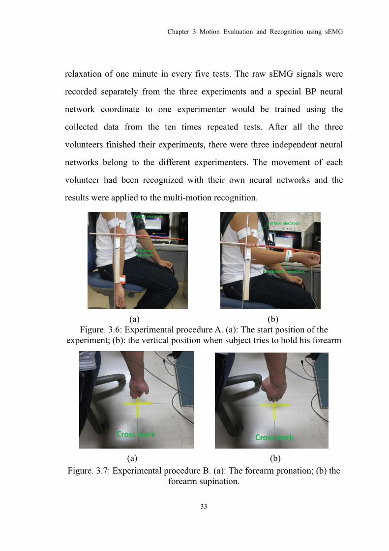
(a) (b) Figure. 3.6: Experimental procedure A. (a): The start position of the
experiment; (b): the vertical position when subject tries to hold his forearm
(a) (b) Figure. 3.7: Experimental procedure B. (a): The forearm pronation; (b) the
forearm supination.

Chapter 3 Motion Evaluation and Recognition using sEMG
34
(a) (b) Figure. 3.8: Experimental procedure C. (a) The palmar flexion; (b) the
palmar dorsiflexion or extension
3.3.1 Experimental results
The experimental results for the first group are listed in Table 3.2. The
confusion plots for the three subjects are shown in Fig. 3.9, respectively.
Table 3.2 Accuracy of artifical neural network
Subject A B C Recognition
rate 81.5 82.1 94.6
(a) Volunteer A (b) Volunteer B (c) Volunteer C
Figure. 3.9: The confusion matrix of the performance

Chapter 3 Motion Evaluation and Recognition using sEMG
35
Recognition results for each volunteer with his own neural network
and with the others are presented in from Fig. 3.10 a to c, where three
different colors of dots stand for the three parameters in the result vector
and the horizontal lines of dashes are critical dividing lines by which all of
the data is separated into ones and zeros. The result vector is described as
follows, where the standard result for up, holding, down and relaxing
movement is (1, 0, 0, 0), (0, 1, 0, 0), (0, 0, 1, 0), and (0, 0, 1, 1)
respectively.
(a). Recognition rate of volunteer A with his own ANN (the left) and with volunteer B’s ANN (the right)
(b). Recognition rate of volunteer B with his own ANN (the left) and with
volunteer C’s ANN (the right)

Chapter 3 Motion Evaluation and Recognition using sEMG
36
(c). Recognition rate of volunteer C with his own ANN (the left) and with
volunteer A’s ANN (the right)
Figure. 3.10: BP ANN recognition results for volunteers with their own ANN and the other’s ANN [65]
As shown at left in Fig. 3.10, results were calculated on line, and were
used as reference input for motor control of the ULERD. As shown in Fig.
3.10 (c), from time intervals 1 to 60, almost all of the dots in group a1,
which represents a1 in equation (10), are positioned above the horizontal
line. After normalization using a piecewise function defined in (11), these
parts of data equaled 1. In contrast, dots in group a2 and the dots in group a1,
are positioned below the horizontal line, equaled 0., These parts of
recognition results consequently represented the vector of (1, 0, 0), which
means the motion of the upper limb up.
The experimental results for the second group are listed in Table 3.3.
The confusion plots for the three subjects are shown in Fig. 3.11,
respectively.
Table 3.3 Accuracy of artifical neural network
Subject A B C Recognition
rate 86.7 85.9 85.4

Chapter 3 Motion Evaluation and Recognition using sEMG
37
(a) Volunteer A (b) Volunteer B (c) Volunteer C
Figure. 3.11: The confusion matrix of the performance.
For the first group experiment, Biceps Brachii (BB) and Triceps
Brachii (TB) muscles were chosen to record sEMG signals. As this pair of
agonist and antagonist muscles take the main charge with the function of
elbow flexion and extension, it is reasonable to choose this pair of muscles
to study the movement of the elbow joint. Because the motion was
performed in sagittal plane, TB was seldom activated. Furthermore, the
involved movement includes concentric contraction motion (elbow flexion),
isometric contraction motion (elbow holding) and active shortening motion
(elbow extension). The muscle status is different among these motions. The
behavior of EMG signals is different according to the different status of
muscle. From this aspect point of view, the AR model used here is to
extract features which represent the status of muscles as well. One set of
the experimental results for AR model feature extraction is depicted in Fig.
3.12. The coefficients were calculated by Burg algorithm.

Chapter 3 Motion Evaluation and Recognition using sEMG
38
Figure. 3.12: Experimental results of features extracted by AR model
As there are 15 features in AR model, only five of these parameters
are plotted in the above figure. It can be indicated, although not very
distinctly, that the changes of features are correspond with the changes of
elbow motion. However, this kind of change decreases with the increasing
of order.
3.4 Improved recognition method
The Neural Network is not an ultra remedy for all the issue of
classification, much less that the Neural Network itself has many trouble
issues. On the other hand, any of the existing classifiers will lose their
function if the features themselves are not separable. It can be indicated
from the experimental results in 3.3.1 that the feathers extracted by AR
model are not stable or distinct. Another problem is with the Neural
Network that it needs many times to train in order to get a proper
classification performance. As it is also mentioned that to improve the
feature extraction method and classifier algorithm is the key factor for
0 50 100 150 200 250 300 350-2
-1.5
-1
-0.5
0
0.5
1
1.5
Sampling Times
Val
ue

Chapter 3 Motion Evaluation and Recognition using sEMG
39
motion recognition.
3.4.1 Support vector machine
SVM is proposed as a classification technique based on maximizing
the margin between a data set and use optimal hyper plane to separate
different data sets [72]. Compared with Neural Network, the advantage of
SVM is that the target parameters depend on finding the optimal solution
for a convex optimization problem, which is described as:
2
1( , ) 0.5
l
ii
cϕ ω ξ ω ξ=
= + ∑ (3-26)
subject to
[( ) ] 1 , 1, 2,...,i i iy x b i lω ξ⋅ + ≥ − = (3-27)
where x is an n-dimensional vector and b is a scalar. c is the independent
variable. l is the number of data points. y is the model to be learned. (3-26)
and (3-27) can be rewritten in the dual Lagrangian form:
1 1 1( ) 0.5 ( , )
l l l
n n m n m n mn n m
L a a a t t k x x= = =
= −∑ ∑∑a (3-28)
where k(xn,xm) denotes the kernel function which plays the soul role in
SVM. To classify new data using the trained model, (3-29) is used based on
the conception of kernel function:
1y( ) ( , )
N
n n nn
a t k x x b=
= +∑x (3-29)
where N denotes the number of support vectors.
One of the challenging issues in SVM is that the solution to a

Chapter 3 Motion Evaluation and Recognition using sEMG
40
quadratic programming problem in M variables in general has
computational complexity that is O(M3). Considering that if there are
10,000 samples, which are just the number of variables in a quadratic
programming problem, and each sample takes a 4-byte float type memory,
a total 3725 GB memories are needed for computation. Fortunately, there is
a popular approach to training SVM, which is called sequential minimal
optimization (SMO) [73]. It is not until the discovery of the effective
training algorithm that SVM has acquired a wide attention.
3.4.2 Improved feature extraction methods
It is intuitive to extract the trend of the EMG signal or finding some
corresponded curve with low changing frequency to represent the changing
for feature extraction.
A Weight Peaks algorithm was designed based on the above concept.
The purpose of WP method is to try to catch the trend of original sEMG
signals [74]. The reconstructed sEMG signals processed by WPT have the
different frequency in different nodes. Therefore, the amount of peaks
obtained in different nodes is different. Zero crossing which is defined as
following is used to find where the peak exists.
1
1 11(sgn( ) )
N
n n n nn
ZC s s s s threshold−
+ +=
= × − ≥∑ ∩ (3-30)
All the reconstructed sEMG signals of zero crossing are saved to
obtain peaks and valleys among them.
The procedure of the WP method is described as following:
If max(sZC(i): sZC(i+1)) + min(sZC(i): sZC(i+1)) ≥ 0

Chapter 3 Motion Evaluation and Recognition using sEMG
41
P(i) = max(sZC(i): sZC(i+1))
Else if max(sZC(i): sZC(i+1)) + min(sZC(i): sZC(i+1)) < 0
P(i) = (-1) × min(sZC(i): sZC(i+1))
where sZC(i) is the reconstructed sEMG signal of zero crossing. P(i)
is the peak or valley between the data of zero crossing and valley is
transformed into positive number.
During experiments, we found that the higher peaks reflect the trend
of motion more than the lower peaks. Therefore the next step of weighted
peaks is to increase the component of higher peak and decrease the
component of lower peak to obtain the feature near to the trend of subject’s
motion. The algorithm is defined in (3-31), where parameter n is defined
experientially.
1 1( 1) ( ) ( 1)nP i P i P in n−+ = + + (3-31)
Actually, it is reasonable to extract the trend from the EMG signal to
represent the feature. The actuator for human motion is the muscle-skeleton
structure and the power is supplied by musculotendon force. Although
EMG signals represents the activation propagation along muscle belly, the
changing frequency of musculotendon force is much lower than that of
EMG signals because of the low-pass-like filter property of the muscle
[30].
Given this consideration, the Hill-type based muscular model was also
applied to extract the feature from the EMG signal. For simplicity, the
Hill-type model can be represented as a linear function of muscle activation

Chapter 3 Motion Evaluation and Recognition using sEMG
42
level, as to be discussed in the next chapter. Before processing raw EMG
signals to muscle activation levels, they usually should be filtered by a
high-pass filter to remove any DC offsets or low-frequency noise and then
rectified. Sometimes, these rectified signals are directly transformed into
muscle activation levels by dividing them by the peak rectified EMG value
obtained during the MVC test. Some researchers [30] suggest that a more
detailed model of muscle activation dynamics is warranted in order to
characterize the time-varying features of the EMG signal. In this paper, a
discretized recursive filter is used.
A discretized recursive filter with a continuous form of a second-order
differential equation was implemented:
2 2( ) ( ) / ( ) / ( )u t Md e t d t Bde t dt Ke t= + + (3-32)
where M, B, and K are the constants that define the dynamics of muscle
activation level and e(t) is the processed EMG signal. This equation can be
expressed in discrete form using backward differences:
1 2( ) ( ) ( 1) ( 2)u t e t d u t u tα β β= − − − − − (3-33)
where d is the electromechanical delay and α, β1, and β2 are the coefficients
that define the second-order dynamics. Selection of the values for α, β1, and
β2 should follow the following restrictions:
1 1 2β γ γ= + (3-34)
2 1 2β γ γ= × (3-35)

Chapter 3 Motion Evaluation and Recognition using sEMG
43
1 1γ < (3-36)
2 1γ < (3-37)
1 2 1α β β− − = (3-38)
in order to guarantee the stability of the equation and that neural activation
does not exceed 1. The calculation results should be filtered by a low-pass
filter (with a cut-off frequency of 3-10 Hz) because the muscle naturally
acts as a filter, resulting in that force changing frequency is much lower
than amplitude changing frequency of EMG signals, which has been
mentioned previously.
3.5 Experimental results
3.5.1 Experimental setup
Seven healthy volunteers (age from 22-28, all male, two left handed
and five right handed) participated in the experiment. The elbow flexion
and extension, forearm pronation and supination and wrist flexion and
extension were the same with experiments in 3.3.1. In the experiment of
wrist adduction and abduction, subjects again relax their upper limbs
vertically as they did in the previous two experiments, and then performed
the adduction and abduction movement (as shown in Fig. 3.13).

Chapter 3 Motion Evaluation and Recognition using sEMG
44
Figure. 3.13: Experiment of wrist adduction and abduction
Each subject repeated the four experiments five times firstly to acquire
data to train classifiers. After classifiers training well, another five trials
were conducted for each of the four experiments to test the on-line
performance of the recognition methods. All the subjects practiced several
times following a standard video before experiments. Flexor carpi radialis,
flexor carpi ulnaris, extensor carpi radialis, extensor carpi ulnaris, biceps
brachii and triceps brachii were selected to record sEMG signals. Apparatus
used in the experiment were the same with the ones in section 3.3.1.
3.5.2 Experimental results
Experimental results of the performance of different combination with
the four feature extraction methods and two classifiers during training
process are listed in Table 3.4. Experimental results shows that WP with
NN obtains the highest recognition accuracy rate (with average of 97.6%)
and RMS with SVM obtains the lowest recognition accuracy rate (with
average of 73.1%). For the feature extraction methods, the performance of
WP and MM is better than that of RMS and DFA while WP is a little better

Chapter 3 Motion Evaluation and Recognition using sEMG
45
than MM (97.6% to 95.1%). For classifiers, NN performs better than SVM
during training process for all the four kinds of features.
Table 3.4. Performance of off-line training. Subject (NN/SVM)
Features A B C D E F G
AR 75.2/74.2 70.7/66.8 82.2/80.5 81.2/78.9 76.1/71.5 70.1/69.7 73.3/70.1
fAR 87.0/82.0 84.1/83.5 90.6/89.5 89.6/86.8 86.5/85.4 82.1/80.2 85.1/81.2
WP 98.4/97.6 97.2/94.1 97.7/94.5 98.9/96.8 97.5/95.2 97.5/94.5 96.5/92.5
MM 98.8/98.0 95.7/90.9 94.1/91.8 91.4/88.3 93.1/90.1 95.3/93.4 97.3/95.4
Experimental results of on-line performance are listed in Table 3.5. It
can still be observed that WP and MM obtain higher recognition accuracy
rate than RMS and DFA while MM is a little higher than WP (94.3% to
92.0%). However, the performance of NN is worse than that of SVM
during on-line testing experiments (except subject D). The recognition
accuracy rates of both of the two classifiers decrease compared with the
performance during training period. The amplitude of decreasing for NN is
larger than that of SVM.
Table 3.5. Performance of on-line testing.
Subject (NN/SVM)
Features A B C D E F G
AR 70.2/74.1 68.7/68.8 80.1/81.5 77.1/78.0 72.1/73.5 70.0/71.1 69.1/71.2
fAR 79.3/83.0 80.1/84.3 82.3/87.1 81.1/85.3 79.1/81.3 75.1/81.1 77.7/80.2
WP 93.4/95.6 89.8/91.1 90.1/91.8 87.1/90.2 90.3/91.0 89.5/91.7 90.5/93.1
MM 94.8/97.0 91.1/93.0 92.1/95.8 93.3/91.3 92.1/93.1 89.3/93.4 92.3/96.4

Chapter 3 Motion Evaluation and Recognition using sEMG
46
Figure. 3.14: On-line testing performance with MM feature extraction
method. (a) shows the classification results by NN. (b) shows the
classification results by SVM.
One set of the on-line testing performance is depicted in Fig. 3.14,
where the blue lines show the classification results and dashed green lines
show the labeled results. The dotted red lines mark the misclassification
results. It can be indicated that the misclassification places are similar
between NN and SVM.
Another important issue for motion recognition is the time
consumption for training and on-line computation, while the latter is more
important than the former in our particular circumstance. Experimental
results for off-line training process are depicted in Fig. 3.15. The
experimental results are average value of off-line training time of the seven
subjects on the same feature extraction method and classifier. The light blue
bars denote the average training time of NN while the green bars denote the
0 5 10 15 20 25 30 35 40 450
2
4
6
Time (s)(a)
Upp
er-li
mb
Mot
ions
0 5 10 15 20 25 30 35 40 450
2
4
6
Time (s)(b)
Upp
er-li
mb
Mot
ions
Classified results by NNLabeled results
Classified results by SVMLabeled results

Chapter 3 Motion Evaluation and Recognition using sEMG
47
ones for SVM. It can be found that NN takes much more time than SVM
(469.6s to 73.5s) to obtain a good performance. For NN, MM and WP takes
more times than RMS and DFA, while the former pair obtains higher
recognition accuracy rate than the latter pair. For SVM, MM and WP takes
fewer times than RMS and DFA, while the former pair still obtains higher
recognition accuracy rate than the latter pair. Experimental results for
on-line calculation are depicted in Fig. 3.16. The blue bars denote the time
consumption for one sample with NN using different feature extraction
methods. There is almost no difference because the structure of the NN is
the same. Compared with NN, it is distinct that it takes much more times
for SVM to complete one recognition loop than NN (1.0918 ms to 0.0034
ms). As the sampling frequency is 1000 Hz in our experiment and this
frequency is also important for sEMG sampling, time consumption longer
than 1 ms will give rise to time delay in real-time experiment. Given this
condition, RMS and DFA, with time consumption of 1.7ms and 1.2ms
respectively, are not suitable for real-time purpose.
Figure. 3.15: Time consumption on off-line training process
MM RMS DFA WP0
200
400
600
800
1000
Tra
inin
g T
ime
(s)
Neural NetworkSupport Vector Machine

Chapter 3 Motion Evaluation and Recognition using sEMG
48
Figure. 3.16: Time consumption for on-line testing process
3.6 Summary
In this chapter, a motion evaluation and recognition with EMG signals
were introduced and discussed. A bilateral training function were proposed,
in which the patient wears our developed ULERD on his/her impaired arm
and performs the upper limb motion bilaterally. The control singles for
ULERD are obtained from the EMG signals recorded from the intact arm.
In order to map EMG signals to motions, the motion recognition based
methods were proposed. Firstly, an AR model based feature extraction
combined with NN classifier method were applied. The recognition
accuracy rate was around 80%. In order to improve the recognition rate and
find the relationship between different feature extraction methods and
classifiers for EMG signals, different combinations of four feature
extraction methods and two classifiers were tested. The proposed muscular
model based method with SVM can acquire a recognition accuracy rate of
above 90% with more motions and fewer training time consumption. The
MM RMS DFA WP0
0.5
1
1.5
2
2.5R
eal-T
ime
Com
putin
g T
ime
(ms)
Neural NetworkSupport Vector Machine

Chapter 3 Motion Evaluation and Recognition using sEMG
49
advantage of the proposed bilateral self-training function is that patients
can perform the training by themselves with the guiding of their intact arm
and the control signals are obtained from EMG signals which are forward
to motions and represent the intention of patients. From the
neurorehabilitation point of view, patients self-inspired motion can bring
more benefit to rehabilitation training than just simple motion following.

Chapter 3 Motion Evaluation and Recognition using sEMG
50

Chapter 4 Continuous Motion Prediction using sEMG
51
Chapter 4 Continuous Motion Prediction
using sEMG
4.1 Introduction
Although accuracy rate for motion recognition method can achieve
above 90%, this kind of method can only provide binary-like control
reference, i.e., it cannot provide exact kinematic value, such as joint angle
of human upper limb, to the controller. In many cases, or maybe most of
the cases, continuous prediction results are more appreciated than
binary-like ones. However, it is a challenging work for all the researchers
to find analytical and quantitative relationship between measured sEMG
signals and desired kinematic variables. The first problem is the
redundancy of human musculoskeletal structure. For a robotic system,
engineering can provide one motor for one degree of freedom, however, in
human body, every degree of freedom, which in many cases is also
complex, is controlled by multiple muscle-tendon pairs. The second
problem is the relationship between sEMG signals and musculotendon
force. The conclusion is still under discussion although some relations have
been studied for particular muscles with different results among researchers.
The third problem is that we cannot detect every concerned muscle with
surface electrode because some muscles are in the deep layer. It seems like
our neural system learned an extremely complex rule to control the
redundant musculoskeletal system.

In
will b
muscu
algorit
proper
4.2 H
Th
genera
describ
where
maxim
coeffic
equals
Th
named
n this chap
be propos
lar model
thm will a
rty of EMG
ill-type b
he Hill
ation from
bed the Hi
F is the lo
mum isom
cient of sh
0.
here is an
d three-elem
Figure.
pter, a con
sed based
l and simp
also be pr
G signals c
based m
model d
m the mech
ill model i
(
oad in the
metric ten
hortening
nother kin
ment mod
4.1: Three
Cha
ntinuous p
d on the
plified mu
roposed to
caused by
muscular
described
hanical po
is shown a
( )(v b F+ +
e muscle; v
sion gene
heat and
nd of des
del which i
e-element
apter 4 Cont
52
prediction
quantitat
usculoske
o conquer
y the differ
model
the mec
oint of vie
as:
) (a b F+ =
v is the ve
erated in
d v0 is th
scription f
is shown i
t Hill-type
tinuous Moti
n method f
tive analy
letal mod
r the prob
rent contra
chanisms
ew. The fa
0 )F a+
elocity of
the mu
e maximu
for Hill-ty
in Fig. 4.1
e muscular
on Prediction
for elbow
ysis using
el. A state
blem of tim
act style o
of musc
famous sta
contractio
scle; a d
um veloci
ype muscu
1.
r model [7
on using sEM
w joint ang
g Hill-typ
te switchin
me-variab
of muscle.
cular for
ate equatio
(4-
on; F0 is th
denotes th
ity when
ular mode
75].
MG
gle
pe
ng
ble
ce
on
-1)
he
he
F
el,

Chapter 4 Continuous Motion Prediction using sEMG
53
Contractile element (CE) represents the active force generation of
muscle. This element is capable of shorting when activated. Series element
(SE) represents the tendon and the intrinsic elasticity of the myofilaments.
It has a soft tissue response and provides energy storing mechanism.
Parallel element represents the passive force of the connective tissues and
also has a soft tissue mechanical behavior. When muscle is at different
status, e.g., different contraction velocity and length, different element
responds differently. The equation described these different elements are
shown following:
, max max(exp( / ) 1) / (exp( ) 1)PE SEF F S L L S= Δ Δ − − (4-2)
maxCE lF F u f f= ⋅ ⋅ (4-3)
( )( )( )0exp -0.5 / 0.05 / 0.19l CE CEf L L= Δ − (4-4)
( )( )( )0
10.1433 0.1074 exp 1.3sinh 2.8 / 1.64v CE CEf V V
−= + − + (4-5)
( )0 max
0.5 1CE CEV u V= + (4-6)
,T CE PE SEF F F= + (4-7)
where SE denotes the passive serial element, CE denotes the active
contractile element and PE denotes the passive element arranged in parallel
to the previous two. ΔL is the change in length of the element with respect
to the slack length, fl is the factor of force introduced by the changes of

Chapter 4 Continuous Motion Prediction using sEMG
54
muscle length and fv is another factor of force introduced by changes of
muscle change velocity. S is a shape parameter, Fmax is the maximum force
exerted by the element for the maximum change in length ΔLmax, and FPE,SE
is the passive force generated by the PE or SE depending on the set of
parameters used. FT is the total force exerted by the muscle. u is the
activation level of a muscle.
One of the problems, as can be easily indicated, is that most of the
parameters involved in the model are hard to measure. In order to apply the
Hill-type model, it is necessary to calibrate these parameters directly or
indirectly.
4.3 Upper-limb musculoskeletal model
From simplification consideration, upper-limb elbow flexion and
extension motion in sagittal plane was studied in this part. The
musculoskeletal model of elbow joint we proposed is depicted in Fig. 4.2.
Figure. 4.2: Musculoskeletal model of elbow joint [76]

Chapter 4 Continuous Motion Prediction using sEMG
55
The distance between the attachment point of the tendon to the
skeleton and elbow joint is l. According to a previous study [24], the tendon
in the upper arm can be regarded as having high stiffness and thus the
tendon deformation is zero. The deformation of the muscle-tendon that
results in elbow rotation can thus be regarded as resulting only from muscle
contraction. The elbow angle θ is the one to be predicted. L is the distance
between the forearm centroid and the elbow joint. In the sagittal plane, it
can be considered that the biceps muscle contracts to pull the forearm
against the force of gravity during the motion of elbow flexion and
extension and that the triceps muscle remains almost unactivated. No
obvious EMG signal changes from the triceps muscle can be observed
during elbow flexion and extension in the sagittal plane. In the transverse
plane, the triceps has to pull the forearm to extend the elbow. As only
voluntary motion in the sagittal plane is discussed, the effect from triceps
brachii is ignored in this paper.
The following equation describes the motion of elbow flexion and
extension in the sagittal plane:
sin sinB f eF l mgL Iθ θ τ θ τ− − = + (4-8)
where FB is the musclotendon force exerted by the biceps and τƒ represents
the torque from frictional effects, which is assumed to be zero in this paper.
τe represents the effects of the environmental interaction, which is also
assumed to be zero because the subjects held nothing in their hands when
they performed the experiments. The mass and inertia of the forearm are m

Chapter 4 Continuous Motion Prediction using sEMG
56
and I, respectively. Dividing (4-8) by lsinθ on both sides yields:
1 1 sinBF mgLl Il θ θ− −= + (4-9)
For (4-9), it is difficult to accurately estimate m and I. However, these
two parameters can be assumed to be constant during a certain period of
time. Using a Hill-type muscular model, the term FB can be represented as
a function of muscular activation level (a), muscle contraction length (Lm),
and muscle contraction velocity (dLm). Equation (4-9) can thus be rewritten
as:
1 1( , , ) sinm mf a L dL c Aθ θ= + (4-10)
where c1 equals mgLl-1 and A1 equals Il
-1.
An actual musculoskeletal model of human upper limb is more
complex than the proposed one, for example not only biceps brachii is
involved in the elbow flexion but also brachialis muscle. The brachialis is
the deep muscle in the upper arm. It is not easy to record EMG signals
from the brachialis using non-invasive surface electrodes. It is assumed that
the muscle synergies involved in a certain motion is invariant under the
same circumstance (such as the same muscle stiffness, motion speed, and
external friction) because the control of the central nervous system keeps
the same. Thus the activation level of biceps brachii can be used to predict
the angle of elbow joint flexion and extension without considering all
involved muscles.

Chapter 4 Continuous Motion Prediction using sEMG
57
4.4 Equation approximation
Because it is quite difficult or impossible, except by extreme approach,
to measure some parameters involved in the dynamic equation, to
approximate these parameters becomes one alternative way. During the
motion of elbow flexion and extension in sagittal plane, tendon can be
regarded as stiff. Given this assumption, ΔLCE in (4-4) can be defined as:
0cos cos cosCE CEL l L Lθ α θ α θΔ = = = (4-11)
where α is the ratio of l to L.
VCE can be defined as:
cos / sinCEV dl dt lθ θ θ= = − (4-12)
According to a previous study [27], VCE0 can be regarded as 10LCE0/s
for the upper limb muscles in most of cases. Given this condition, the
following equation is obtained:
0
0 0
sin0.1 sin
10CECE
CE CE
LVV L
θα θαθ θ= − = − (4-13)
Substituting (4-12) and (4-13) back into the Hill-type model and rewriting
the term FB with the detailed equations yields:
max 1 1(cos ) ( ,sin ) sinl vF a f f C Aθ θ θ θ θ⋅ ⋅ = + (4-14)
Taking the natural logarithm of both sides yields:
1 22 1 1 3ln(exp( ) 1) ln( ( ,sin )) ln( sin ) ( cos 0.05)vC uR f A c Cθ θ θ θ α θ−+ − + = + + − (4-15)

Chapter 4 Continuous Motion Prediction using sEMG
58
where C2 and C3 equal ln(Fmax(exp(A)-1)-1) and 0.5×0.19-2, respectively.
The value of term lnfv(dθ,sinθ) is around zero in this circumstance, and thus
ignored. Since the value of c1 is much larger than that of A1d2θsinθ, the
term ln(A1d2θsinθ+c1) can be simplified as lnc1 and we use C1 to instead for
the purpose of keeping mathematic unification. Equation (4-15) can thus be
further simplified as:
1 22 1 3ln(exp( ) 1) ( cos 0.05)C uR C C α θ−+ − = + − (4-16)
where u represents the muscle activation level, which can be calculated
from EMG signals, and θ is the upper limb elbow joint angle.
In (4-16), the term ln(exp(uR-1)-1) can be represented as a quadratic
polynomial with variable uR-1. Then, (4-16) can be transformed into Eq.
(4-17), which has a quadratic-like relationship between cos2θ and uR-1.
According to the experimental results (discussed in the next section), this
quadratic-like relationship is extremely strong during the upper limb elbow
flexion period.
2 1 22 1 30
( ) ( cos 0.05)i
iiC a uR C C α θ−
=+ = + −∑ (4-17)
4.5 State switch algorithm
Although the relationship between EMG signals (muscle activation
level) and elbow joint angle seems simple from (4-17), the actual relation is
more complicated. Figure 4.3 shows one set of experimental results of
normalized muscle activation level during the motion of elbow flexion and
extension. There are four periods: relaxation period, elbow flexion period
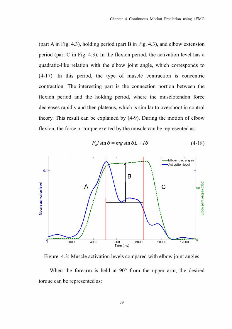
Chapter 4 Continuous Motion Prediction using sEMG
59
(part A in Fig. 4.3), holding period (part B in Fig. 4.3), and elbow extension
period (part C in Fig. 4.3). In the flexion period, the activation level has a
quadratic-like relation with the elbow joint angle, which corresponds to
(4-17). In this period, the type of muscle contraction is concentric
contraction. The interesting part is the connection portion between the
flexion period and the holding period, where the musclotendon force
decreases rapidly and then plateaus, which is similar to overshoot in control
theory. This result can be explained by (4-9). During the motion of elbow
flexion, the force or torque exerted by the muscle can be represented as:
sin sinBF l mg L Iθ θ θ= + (4-18)
Figure. 4.3: Muscle activation levels compared with elbow joint angles
When the forearm is held at 90° from the upper arm, the desired
torque can be represented as:

Chapter 4 Continuous Motion Prediction using sEMG
60
, ( 90 )BF l mgL θ= = (4-19)
Compared with (4-19), there is an extra acceleration term in (4-9),
resulting in a higher force level in the elbow flexion period. As the muscle
activation level directly reflects the musclotendon force, the activation
level is higher in the flexion period than in the holding period. Another
reason is the transformation of muscle contraction type from concentric to
isometric. However, this issue is beyond the scope of this paper. During the
period of elbow extension, the muscle activation level decreases with
decreasing elbow joint angle. Furthermore, during the extension period, the
muscle contraction type changes to active shortening.
Given this situation, a state switching model (as shown in Fig. 4.4) is
developed for elbow joint angle prediction. The input of this switching
model is the muscle activation level. There are four states in this state
switching model, namely relaxation, flexion, holding and extension states,
which correspond to the elbow joint motions with the same names. The
relaxation state is the initial state, at which the forearm is 180° from the
upper arm in the sagittal plane. When the muscle activation level increases,
the state changes to the flexion state. The flexion state changes to the
holding state only when the activation level stops increasing and the value
exceeds a threshold. When the level decreases, the state changes to the
extension state. In the holding state, the state can only change to the
extension state when the activation level starts to decrease. The extension
state changes to the relaxation state when the value of the activation level
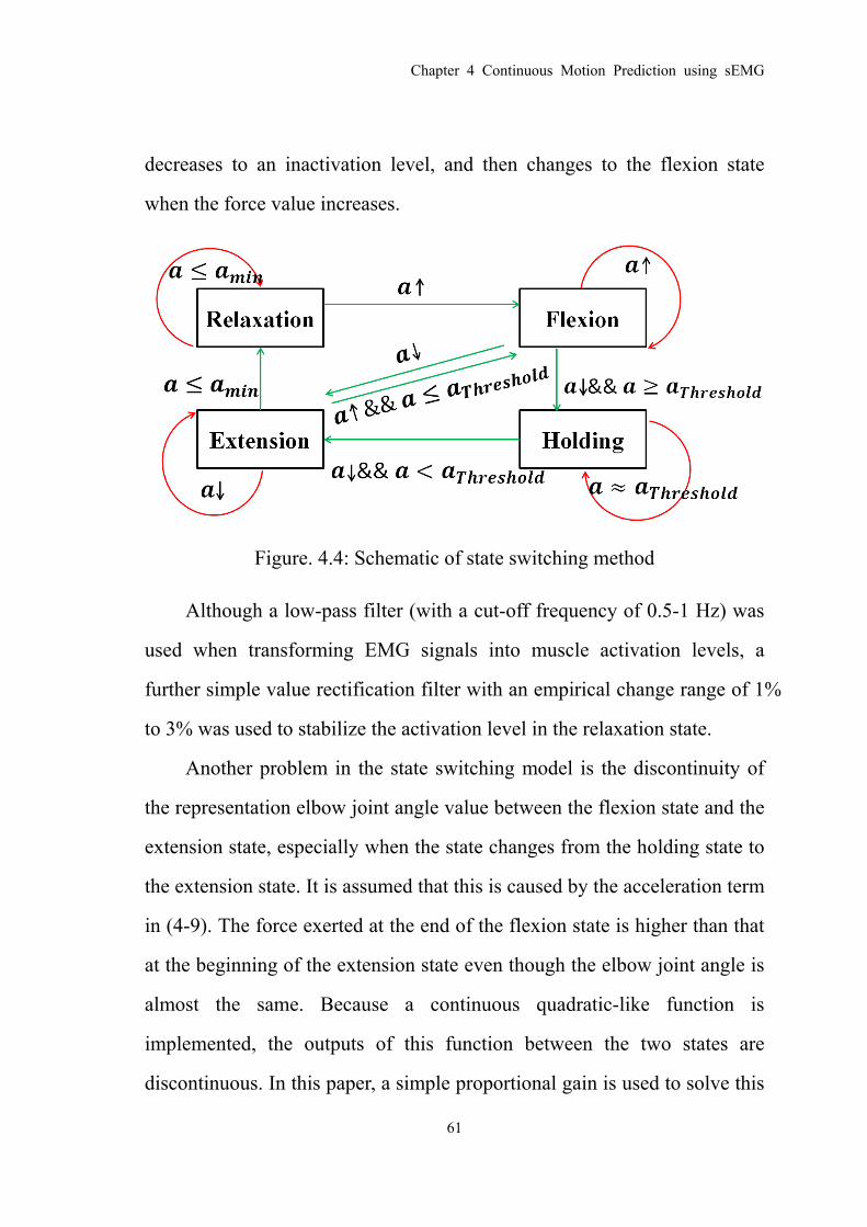
Chapter 4 Continuous Motion Prediction using sEMG
61
decreases to an inactivation level, and then changes to the flexion state
when the force value increases.
Figure. 4.4: Schematic of state switching method
Although a low-pass filter (with a cut-off frequency of 0.5-1 Hz) was
used when transforming EMG signals into muscle activation levels, a
further simple value rectification filter with an empirical change range of 1%
to 3% was used to stabilize the activation level in the relaxation state.
Another problem in the state switching model is the discontinuity of
the representation elbow joint angle value between the flexion state and the
extension state, especially when the state changes from the holding state to
the extension state. It is assumed that this is caused by the acceleration term
in (4-9). The force exerted at the end of the flexion state is higher than that
at the beginning of the extension state even though the elbow joint angle is
almost the same. Because a continuous quadratic-like function is
implemented, the outputs of this function between the two states are
discontinuous. In this paper, a simple proportional gain is used to solve this

Chapter 4 Continuous Motion Prediction using sEMG
62
problem:
max
max`p θ
θ= (4-20)
where θmax is the elbow joint angle at the end of the flexion state and θ`max
is the elbow joint angle at the beginning of the extension state. According
to the definitions of flexion and extension states, the last value at the end of
the flexion state is the maximum elbow joint angle at the flexion state and
the first value at the beginning of the extension state is the maximum elbow
joint angle at the extension state.
In the pre-processing step, raw EMG signals are filtered by a
high-pass fourth-order Butterworth filter with a cut-off frequency of 10 Hz
and then are processed using (3-33) to get the feature estimation of u(t).
After u(t) is filtered with a low-pass second-order Butterworth filter (with
0.5-1 Hz cut-off frequency), the results are divided with the value acquired
from MVC test to obtain the muscle activation level (a). Then, the
activation level is rectified by 1-3% to reduce the drifting effect caused by
the characteristics of EMG signals. The rectified activation level is used as
the input to the proposed state switching model to obtain a representation
of the elbow joint angle, which is used as the control reference input for the
exoskeleton device. The proposed Hill-type-based muscular model is
combined in the state switching method.
4.6 Experimental results
4.6.1 Experimental setup
Ten healthy volunteers (age: 24.60±1.67 years, height: 1.70±0.07 m,

Chapter 4 Continuous Motion Prediction using sEMG
63
weight: 67.66±9.54 kg, two female, eight male, two left-handed, and eight
right-handed) participated in the experiments. Process of attaching
electrodes is the same with section 3.3.1. The sampling rate was 1000 Hz
with differential amplification (gain: 1000) and common mode rejection
(104dB). A fourth-order high-pass Butterworth filter with a 10-Hz cut-off
frequency was implemented in software to remove the DC offsets in EMG
signals before they were rectified. The user interface was programmed
using Visual C++ 2010 (Microsoft Co., USA). The analog/digital (A/D)
data from the A/D board was collected through the application
programming interface and processed with MATLAB (The MathWorks Co.,
USA). The software was run on a personal computer with a 2.8-GHz
quad-core processor (Intel Core i7 860) and 4 GB of RAM. An MTx sensor
(Xsens Technologies B.V., USA) was attached on the subject’s forearm to
record the elbow joint angle for calibration and comparison.
A maximum voluntary contraction (MVC) test at the isometric
contraction condition was performed before the experiment. Subjects were
asked to hold a dumbbell (from 3 to 18 kg) at an angle of 90° between their
upper arms and forearms and the EMG signals from the biceps muscle
were recorded. Five trials were performed to determine the MVC EMG
value. A sufficient rest time between the five trials was provided to avoid
muscle fatigue.
In the experiment of upper limb flexion and extension in the sagittal
plane, the subjects were asked to start with both side of their arms relaxed
vertically and then flex their forearms to 90°. After having maintained their

Chapter 4 Continuous Motion Prediction using sEMG
64
forearms in the horizontal position for 3 s, the subjects were asked to
extend their forearms to the initial vertical position. Then, a calibration
calculation for proposed method was performed offline. After the
calibration was finished, the subjects were asked to perform the movement
repetitively. A real-time simulation results were conducted on the personal
computer by a self-developed software with VS 2010 and OpenGL (as
shown in Fig. 4.5).
Figure. 4.5: On-line experiment of controlling a virtual arm
Furthermore, a consecutive stepping test was performed by five of the
ten subjects. In the consecutive stepping test, the subjects were asked to
move their active upper limb to angle of 30°, 20°, and 10°, respectively,
and hold for 3 seconds at each step.
A photograph of each subject was taken to record the electrode
position on the upper arm. The condition of upper limb movement, such as

Chapter 4 Continuous Motion Prediction using sEMG
65
forearm rotation speed and upper arm stiffness, should be restricted for the
accurate offline calibration. In order to keep the rotation speed and
generalize upper limb movement, the subjects were asked to practice the
motion by following a prerecorded video. All motions were voluntary
without any external force applied on the upper limb. Each subject repeated
the three experiments ten times with a relaxation time of 1 min between
tests.
4.6.2 Experimental results
To evaluate the proposed musculoskeletal model, all recorded data
from the ten subjects during the four days were fitted using the curve fitting
tools of MATLAB with quadratic polynomial equations. The inputs were
values of the muscle activation level during the flexion motion and the
outputs were values of cos2θ. Some bad data caused by electrodes sliding
on the skin surface were ignored. Figure 4.6 shows one set of model
evaluation results from the ten subjects. The dashed lines are the results
calculated with data recorded from EMG electrodes (to get the muscle
activation level) and from the MTx sensor (to get elbow joint angles). The
solid lines are prediction results based on the proposed model. Table 4.1
lists detailed information (mean ± standard deviation). The experimental
results show that the average values of the correlation coefficient is above
0.97 for all ten subjects. Although a linear relationship between muscle
activation level and cos2θ was found for some subjects (in Fig. 4.6, subjects
B and F have correlation coefficients of 0.95 and 0.94, respectively), the
quadratic-like relationship has a higher correlation coefficient (with

Chapter 4 Continuous Motion Prediction using sEMG
66
correlation coefficients of 0.97 and 0.98) than that of the linear one in the
same case. In other cases (in Fig. 4.6, subjects I and J), the quadratic-like
relationship is more suitable (linear relationship has correlation coefficients
of 0.86 and 0.85 and quadratic-like one has 0.97 and 0.98).
Table 4.1 Correlation coefficients between experimental data and proposed model
Day Subject
A B C D E F G H I J
1 0.99±0.01 0.99±0.01 0.98±0.01 0.98±0.01 0.99±0.00 0.98±0.01 0.98±0.01 0.98±0.01 0.97±0.02 0.98±0.01
2 0.98±0.01 0.98±0.01 0.98±0.01 0.98±0.01 0.98±0.01 0.98±0.01 0.98±0.02 0.99±0.01 0.97±0.01 0.97±0.01
3 0.99±0.01 0.97±0.02 0.97±0.02 0.99±0.01 0.97±0.02 0.97±0.01 0.99±0.01 0.97±0.02 0.97±0.01 0.98±0.01
4 0.98±0.01 0.99±0.01 0.97±0.01 0.99±0.01 0.99±0.01 0.98±0.01 0.98±0.01 0.98±0.02 0.97±0.01 0.97±0.01
Figure. 4.6: Model validation results of the ten subjects
Figure 4.6 shows one set of the elbow joint angle prediction results
obtained using the proposed method. The calculated elbow joint angles are
plotted with a solid line and the recorded elbow joint angles obtained using
0.04 0.045 0.050
0.2
0.4
0.6
0.8
1
Subject A0.05 0.06 0.07
0
0.2
0.4
0.6
0.8
1
Subject B0.04 0.05 0.06 0.070
0.2
0.4
0.6
0.8
1
Subject C0.04 0.045
0
0.2
0.4
0.6
0.8
1
Subject D0.042 0.044 0.046
0.2
0.4
0.6
0.8
1
Subject E
0.042 0.044 0.0460.2
0.4
0.6
0.8
1
Subject F0.045 0.05 0.0550
0.2
0.4
0.6
0.8
1
Subject G0.03 0.04 0.050
0.2
0.4
0.6
0.8
1
Subject H0.035 0.04 0.0450
0.2
0.4
0.6
0.8
1
Subject I0.03 0.035 0.040
0.2
0.4
0.6
0.8
1
Subject J

Chapter 4 Continuous Motion Prediction using sEMG
67
the MTx sensor are plotted with a dashed line. Trajectory of the
exoskeleton device is plotted with a dotted line. The different states are
divided using black lines. In state 1 (relaxation state), the prediction results
and recorded results are all zero. Actually, small changes in the muscle
activation level can be observed in this period due to the small changes in
EMG signals. These small changes may make the current state change to
the next state and cause errors. A rectification method is thus implemented
to stabilize the changes. In state 2 (flexion state), there is usually a time lag
(about 100-200 ms) at the end of this state between the recorded data and
prediction results. This time lag is caused by the transition from the flexion
state to the holding state. The flexion state changes to holding state when
the input (the muscle activation level) for the state switching exceeds a
threshold, which is pre-determined. However the real desired threshold
changes with the variation of EMG signals. As a consequence, the constant
pre-determined threshold makes the prediction of holding state backwardly.
In state 3 (holding state), the elbow joint remains in a certain position (75°
in this case). When the state changes to the extension state, the values of
prediction results decrease with decreasing muscle activation level. The
correlation coefficients and root-mean-square (RMS) errors between
prediction results and recorded ones of the ten subjects are listed in Table
4.2.

Chapter 4 Continuous Motion Prediction using sEMG
68
Figure 4.7: Experimental results of continuous elbow joint angle prediction method
Table 4.2 Experimental results of the ten subjects
(a) Correlation coefficients
Day Subject
A B C D E F G H I J
1 0.96±0.02 0.91±0.01 0.94±0.03 0.95±0.01 0.98±0.02 0.96±0.01 0.96±0.07 0.97±0.02 0.94±0.09 0.93±0.05
2 0.98±0.01 0.92±0.05 0.94±0.05 0.95±0.04 0.95±0.04 0.96±0.03 0.98±0.04 0.97±0.03 0.97±0.01 0.97±0.03
3 0.98±0.04 0.91±0.09 0.93±0.07 0.93±0.06 0.95±0.05 0.91±0.08 0.94±0.06 0.97±0.02 0.94±0.01 0.92±0.01
4 0.94±0.06 0.95±0.04 0.97±0.01 0.95±0.07 0.94±0.06 0.97±0.01 0.92±0.08 0.95±0.05 0.95±0.01 0.96±0.02
(b) RMS errors (degrees) between prediction results and recorded results
Day Subject
A B C D E F G H I J
1 9.78±3.79 8.10±2.59 5.20±2.80 9.22±2.12 5.60±0.34 9.17±2.80 9.47±1.37 9.70±0.13 8.64±1.60 5.33±1.27
2 7.33±2.14 7.56±2.31 4.32±2.21 7.31±3.31 5.55±1.21 7.78±2.57 8.33±2.12 9.05±2.11 5.31±2.21 4.21±3.17
3 6.23±4.11 7.71±2.77 5.78±3.33 8.21±2.23 6.04±2.11 7.31±2.23 7.78±3.16 7.73±3.01 7.04±2.13 5.78±2.00
4 7.35±2.11 8.78±2.11 4.32±2.45 5.45±3.13 5.57±3.14 5.32±2.85 9.01±2.11 7.00±1.31 6.66±3.01 6.05±1.15
0 2000 4000 6000 8000 10000 120000
10
20
30
40
50
60
70
80
Time (ms)
Join
t ang
le (d
eg)
Predicted Elbow Joint AngleRecorded Elbow Joint Angle
State 1 State 2 State 3 State 4

Chapter 4 Continuous Motion Prediction using sEMG
69
Nevertheless, the proposed state switching model may give rise to
distortion or time lag in some cases. In Fig. 4.8, the motion is forearm
flexion and then extension, without a holding period during flexion and
extension. There is a time lag between the flexion and extension in the
prediction results. This is because the state changes from flexion to holding
and then to extension. It takes some time (as long as the time lag) for the
model to change state from holding to extension. This time lag depends on
the decreasing rate of EMG signals (γ), the difference between peak muscle
activation levels (aP), the threshold set for the holding state, and a range
value (ar: 1-3%) that is used to reduce the influence of the non-stationarity
of EMG signals. The time lag can be defined as:
(1 )p t rlag
F F at
γ− −
= (4-21)
where the only parameter which can be controlled is ar. However the
influence of ar is much less than that of the other parameters. Thus, this lag
can be regarded as an inherent defect of this model caused by the
non-stationarity of EMG signals. Although this time lag appears in certain
circumstances, it does not affect all results, i.e. this lag, does not
accumulate in the state switching method.
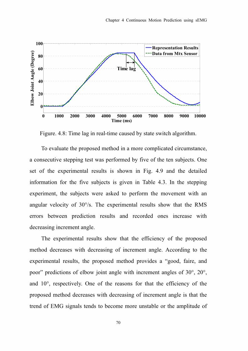
Chapter 4 Continuous Motion Prediction using sEMG
70
Figure. 4.8: Time lag in real-time caused by state switch algorithm.
To evaluate the proposed method in a more complicated circumstance,
a consecutive stepping test was performed by five of the ten subjects. One
set of the experimental results is shown in Fig. 4.9 and the detailed
information for the five subjects is given in Table 4.3. In the stepping
experiment, the subjects were asked to perform the movement with an
angular velocity of 30°/s. The experimental results show that the RMS
errors between prediction results and recorded ones increase with
decreasing increment angle.
The experimental results show that the efficiency of the proposed
method decreases with decreasing of increment angle. According to the
experimental results, the proposed method provides a “good, faire, and
poor” predictions of elbow joint angle with increment angles of 30°, 20°,
and 10°, respectively. One of the reasons for that the efficiency of the
proposed method decreases with decreasing of increment angle is that the
trend of EMG signals tends to become more unstable or the amplitude of
0 1000 2000 3000 4000 5000 6000 7000 8000 9000 10000
0
20
40
60
80
100
Time (ms)
Elb
ow J
oint
Ang
le (D
egre
e)
Representation ResultsData from Mtx Sensor
Time lag

Chapter 4 Continuous Motion Prediction using sEMG
71
ripple of EMG signals tends to become wider with decreasing increment
angle. The wide ripple of EMG signals directly influences the calculation
of muscle activation level, i.e., there are ripples in muscle activation levels.
The activation levels thus become unstable as well. This phenomenon was
found for all five subjects during the consecutive stepping test. But this
kind of phenomenon doesn’t appear in the continuous motion test. This
phenomenon indicates that the subject must provide more effort to achieve
the task in the consecutive stepping text than in the continuous motion text
and the fluctuation in EMG signals during consecutive stepping test reflects
upon this effort. According to the experimental results, the proposed
method can provide suitable predictions within increments of 20° to 30°.
(a)
0 1 2 3 4 5x 10⁴
0
10
20
30
40
50
60
70
80
90
Time (ms)
Elb
ow J
oint
Ang
le (D
egre
e)
Representation ResultsRecorded data from Mtx sensor

Chapter 4 Continuous Motion Prediction using sEMG
72
(b)
(c)
Figure. 4.9: Consecutive stepping test results for different increment angles.
(a) with increment of 30°; (b) with increment of 20°; (c) with increment of
10°.
0 1 2 3 4 5 6 7x 10⁴
0
10
20
30
40
50
60
70
80
90
Time (ms)
Elb
ow J
oint
Ang
le (D
egre
e)
Representation resultsRecorded data from Mtx sensor
0 1 2 3 4 5 6 7 8 9x 10⁴
0
10
20
30
40
50
60
70
80
90
Time (ms)
Elb
ow J
oint
Ang
le (D
egre
e)
Representation resultsRecorded data from Mtx sensor

Chapter 4 Continuous Motion Prediction using sEMG
73
Table 4.3 RMS errors between prediction results and recorded results in consecutive stepping test
Increment Subject
A C E G I
30 4.40±3.15 5.40±2.21 6.51±3.11 5.32±4.21 6.71±4.00
20 6.61±3.71 8.83±4.94 7.139±3.90 9.21±2.11 8.31±3.57
10 15.40±3.15 17.40±3.12 17.35±4.12 19.35±3.15 17.44±4.23
4.5 Summary
In this chapter, a continuous prediction method for elbow joint angle
was proposed, which is one of the new points in my study. This method
aimed to solve the problem that motion recognition based method can only
provide binary-like results for control. The proposed method was based on
the quantitative analysis of sEMG signals and corresponded elbow position
within movement. The dynamic equation was developed on Hill-type
muscular model and simplified elbow joint musculotenedon model. With
approximation and some assumptions, a quadratic expression was found
and evaluated by a four-day-long experiment on ten subjects. A state
switching model was developed to avoid the influence of acceleration and
transit between muscle contraction states. A consecutive stepping
experiment was conducted to test the feasibility of the proposed method
with more free motion. Experimental results indicate that this method can
provide suitable prediction results with RMS errors of below 10° in
continuous motion and RMS errors of below 10° in stepping motion with
20° and 30° increments. With this method, our ULERD can follow the

Chapter 4 Continuous Motion Prediction using sEMG
74
motion of subject in real-time, not just by pre-defined motions controlled
by switch signals. One point should still be noticed that the proposed
method is focused on elbow joint, where musculoskeletal structure is
relative simple and involved muscles are fewer, compared with the other
joints. There is a long way to go if we tend to extend this kind of method on
the other joints.

Chapter 5 Force Evaluation and Prediction using sEMG
75
Chapter 5 Force Evaluation and Prediction
using sEMG
5.1 Introduction
In this chapter, the relation between force exerted by subject and
sEMG signals will be discussed. A prediction method for contact force
between subject and the environment will be proposed to provide remote
force evaluation function in our home-used rehabilitation system.
The relation between musculotendon force and EMG signals is more
direct than the one concerned about motions, as motions are also involved
by external variables, e.g., gestures, gravity and status of tendon. However,
that is not to say the relation between musculotendon force and EMG
signals is simpler. It is still complex, even in a solo isolated muscle.
Although the popular Hill-type or Huxley-type muscular models provide a
way to explain the force generation function in a muscle, the models
themselves are too complex to be directly applied. Nevertheless, there are
some arguments about these models that the conclusions were obtained
from experiments conducted on isolated muscles which property is
different from the one in a living body. It is not hard to tell that to measure
the data under a ‘perfect’ condition is quite difficult.
However, it is just the case that using EMG signals is more direct and
convenient to predict musculotendon force. Usually, the measurement of
muscular force normally cannot be performed by indwelling force

Chapter 5 Force Evaluation and Prediction using sEMG
76
transducers inserted into the tendon but rather by quantifying the reaction
force supplied to external loads or ‘‘mechanical ground”. However in some
cases it is inconvenient to attach sensors on the surface of the contacting
environment. On the other hand, the measurement results from the sensors
are the output of the corresponded musculoskeletal system, which is hard to
reflect the situation of the individual muscle. On the contrary, using EMG
can observe the individual muscle and predict the output of the
musculoskeletal system without using a force sensor.
5.2 Muscular model
In this chapter, I focus on two motions: downward touch motion and
push motion, given the two motions are very common in daily living. As
the redundancy and complex of human musculoskeletal system, only
isometric contraction was considered, i.e., subject kept still when he
exerted force on the object. EMG signals were recorded from the flexor
carpi radialis (FCR), the flexor carpi ulnaris (FCU), the extensor carpi
radialis longus (ECRL), the extensor carpi ulnaris (ECU), the extensor
digitorum (ED), the biceps brachii (BB), the triceps brachii (TB), and the
pectoralis major (PM). These eight muscles are involved in the studied
motions. Given these conditions, two muscle-skeleton models were used to
derive the dynamic equations for the two motions, respectively.
The sketch of the musculoskeletal model for the downward touch
motion is shown in Fig. 5.1 (a) while the one for push motion is shown in
Fig. 5.2 (a). The figures on the right column show the corresponded
changings of forces for the two motions, respectively. There are mainly

Chapter 5 Force Evaluation and Prediction using sEMG
77
three degree of freedoms (DoFs) on the forearm which are
pronation/supination of the forearm, radial/ulnar deviation around the wrist
and palm flexion and extension. In our special case of downward touch
motion, only palm flexion and extension was concerned. The pairs of
flexors and extensors around the forearm act to keep the stiffness of wrist
joint and balance the torque from the contact motion. As the motion is
isometric, the dynamic function can be written as:
lexor xtensor-F E mg Fτ τ τ τ+ = (5-1)
where τFlexor denotes the torque derived by the flexors while τExtensor denotes
the torque derived by extensors. τF is the torque derived by the contact
force. τmg is the torque derived by the gravity force of hand. The friction in
the joint is ignored here. The singular gesture, in which upper arm and
lower arm form in a line, was tried to avoid. In singular condition, the
direction of the contact force pass through the wrist joint. Under this
circumstance, the main function of flexors and extensors around the
forearm is to maintain the stiffness of the wrist joint, and contact force is
balanced by the contraction from the other muscle groups.
In push motion, the contact force exerts through the wrist joint (as
shown in Fig. 5.2 (a)). This equals an identical force (F’) exerts on the
elbow joint and couples an additional torque (τf) on the forearm. In this case,
the contact force also generates a torque on the shoulder joint (τs). The BB
and TB contract to balance the torque (τf) exerted on the forearm. PM
contract to balance the torque (τs) exerted on shoulder joint. The dynamic

Chapter 5 Force Evaluation and Prediction using sEMG
78
function can be written as:
-Ag Antτ τ τ= (5-2)
f SF F F= + (5-3)
where τAg denotes the vector of torque generated by agonist muscles and
τAnt denotes the vector of torque generated by antagonist muscles. τ is the
vector with the form of (τf , τs). F is vector of the desired push force. Ff
and Fs can be calculated from the torque equation.
All torques in (5-1) and (5-2) can be expressed as the forces (muscular
forces or gravity force) product the corresponded moments. Because the
motions are isometric, the moments involved in the equations can be
considered as constant. Therefore, (5-1) and (5-2) can be written in a
compact form of:
i iFτ α= ⋅∑ (5-4)
where αi denotes the constant moment. It should be noticed that subjects
were asked to try to perform the motion with the same gesture for each
time. Because of the redundancy of human musculoskeletal structure, a
motion can be executed with different gestures. The moment arms or
muscle status will be different if the gestures are different. Given this
condition, the gesture for each motion was constrained. Subjects were
asked to perform the motion with a comfortable gesture and keep the same
gesture for each time.

Chapter 5 Force Evaluation and Prediction using sEMG
79
(a) (b)
Figure. 5.1 Downward touch motion. (a) shows the musculoskeletal model
and (b) shows the corresponded force.
(a) Musculoskeletal model
(b) Changing of forces
Figure. 5.2: Push motion
-0.50
0.5
02
46
810
0
0.1
0.2
0.3
0.4
0.5
0.6
0.7
0.8
0.9
1
Z-A
xis
Touc
h Fo
rce
(N)
X-Axis Touch Force (N)
Time (s)
0
2
4
6
8
10
01
23
45
67
8
-4
-2
0
2
Z-A
xis
Push
For
ce (N
)
Time (s) X-Axis Push Force (N)

Chapter 5 Force Evaluation and Prediction using sEMG
80
The Hill-type muscular model as introduced in section 4.2 was applied
again to predict the musculotendon force with EMG signals. Under the
condition of isometric contraction, the term of Fi in (5-4) can be instead
with a linear expression of muscle activation level, and (5-4) can thus be
rewritten as:
i i uτ α β= ⋅ ⋅∑ (5-5)
It should be noticed here that a linear relation between muscle activation
level and musculotendon force was assumed, which was not very precise
and may be different from individuals. However this assumption is
reasonable within a certain range of motion.
5.3 Motion recognition
As dynamic equations are obtained, the time point to apply these
equations is needed. A neural network classifier was applied to recognize
the motions. As has been discussed in Chapter 3 that SVM costs more time
than NN on real-time computation, NN was adopted in this thesis because I
do not want to take too much time on motion classification. The inputs
were processed EMG signals or muscle activation levels obtained from five
muscles, which were BB, TB, FCR, ECRL and ECRB. The outputs of the
classifier were binary representation for four motions, which are relaxing,
downward touching, pushing, and exerting force motion. Therefore, the
input was a vector with five components and the output was a vector with
four components. The training data were well labeled, according to the
values from MTx sensors and 6-axis force sensor. One set of the

Chapter 5 Force Evaluation and Prediction using sEMG
81
experimental data (push motion) is shown in Fig. 5.3. The relaxing motion
was labeled when there were no changings in the value from MTx sensors
and no muscle activation level. The pushing motion or touch motion was
labeled when there were changings in values from MTx sensors and no
changing in force value. The exerting force motion was labeled when force
value changes.
There was one hidden layer with seven neurons in the neural network.
The hyperbolic tangent sigmoid transfer function and scaled conjugate
gradient backpropagation training algorithm were adopted for hidden layer
combination and learning process, respectively.
Figure. 5.3: One example of the push motion
5.4 Parameter calibration
The Bayesian linear regression (BLR) algorithm [80] was adopted to
calibrate the parameters (ωi) in the dynamic equations.
Assuming that the noise in prediction function is with the form of
0 1000 2000 3000 4000 5000 6000 7000 8000 9000 100000
0.1
0.2
Nor
mal
ized
EM
G
0 1000 2000 3000 4000 5000 6000 7000 8000 9000 100000
10
20
30
Inte
ract
ion
Forc
e (N
)
0 1000 2000 3000 4000 5000 6000 7000 8000 9000 10000-100
0
100
Time (ms)
Join
t Ang
le (D
egre
e)
Wrist JointElbow Joint
BBTBFCRECRLECRB
Force exerting Motion
Relaxing Relaxing
Push Motion
Push Motion

Chapter 5 Force Evaluation and Prediction using sEMG
82
Gaussian, the proposed dynamic equation (5-5) can be written as:
( , )y ε= +t a ω (5-6)
where ε is a zero mean Gaussian random variable with precision β. Thus
the following likelihood function can be obtained:
1
1
( | ( ), )( | , , )N
nn
N t up ϕβ β −
=
= ∏t a Τω ω (5-7)
On the other hand, we assume that the prior probability distribution over ω
is also with the form of Gaussian distribution:
0 0( | )( ) Np = m S,ω ω (5-8)
where m0 denotes the mean value of ω and S0 denotes the covariance.
Because the posterior distribution is proportional to the product of the
likelihood function and the prior, the following function is obtained:
| ( | )( ) N NNp =t m S,ω ω (5-9)
where
10 0( )T
N N β−= + Φm S S m t (5-10)
1 10
TN β− −= + Φ ΦS S (5-11)
The mN denotes the mean of ω given the condition of t, and SN is the
covariance. The evidence approximation method was adopted to calculate
mN and SN. A “cross-validation” selection criteria was adopted to obtain
local optimal parameters. In the “cross-validation” criteria, one set of the

Chapter 5 Force Evaluation and Prediction using sEMG
83
experimental data was used to calculate the parameters and the
performance of these parameters was assessed by evaluating the
root-mean-square (RMS) errors with the remaining data. This procedure
was performed on all the experimental data and the ones with the smallest
RMS errors were selected as the final optimal parameters.
It should be noticed that the term ‘global’ used here means the entire
sEMG data recorded from the target muscles during all the corresponded
force exerting motion in a relative long period of one subject’ ADL. It can
be easily noticed that it is almost impossible. The term ‘local’, on the
contrary, means one set of experimental data for just one or limited number
of trials. I tried to use BLR to obtain the global or ‘almost global’ optimal
parameters from a limited number of local data. This concept is based on
the assumption that there is a constant ‘pattern’ existing in the sEMG data
during our expected period and all the data surround the ‘pattern’ with a
kind of probability distribution. Although this probability distribution, if
existing, is not Gaussian, it is reasonable and nature to assume that the
Gaussian is the most-likely one, because there are many uncertain complex
‘disturbances’ exerting on the EMG signals.
5.5 Experimental results
5.5.1 Experimental setup
Five subjects (age: 26.00±1.73 years, height: 1.72±0.04 m, weight:
66.40±10.36 kg, all male, one left-handed, and four right-handed)
participated in the experiment. The maximum voluntary contraction (MVC)
test was performed for each subject to record the maximum amplitude of

Chapter 5 Force Evaluation and Prediction using sEMG
84
EMG signals for each muscle. As the high redundancy and complexity of
human musculoskeletal system, isometric downward touch motion and
push motion are considered in this paper. The downward touch motion is
defined as that subject uses his figure tips to exert force on the environment
with palmar aspect facing downward while the shoulder joint is around 20°,
elbow joint around 10°, and wrist joint around 45° in sagittal plane (as
shown in Fig. 5.4 (a)). The push motion is defined as that subject uses his
palmar to push the object with the shoulder joint around 30°, elbow joint
around 100°, and wrist joint around 40° in sagittal plane (as shown in Fig.
5.4 (b)). The experiment for downward touch motion was divided into three
trials, with maximum force amplitude of 5 N, 10 N and 15 N, respectively,
and there were five trials in experiment of push motion, range from 5 N to
25 N, with an increment of 5 N. During each trial, the subject was asked to
contact the object for 2 to 3 s. The subject repeated each trial 10 times with
a relaxation time of 1 min between tests.
(a) Downward touch motion (b) Push motion
Figure. 5.4: Gestures for the two motions

Chapter 5 Force Evaluation and Prediction using sEMG
85
A remote contact force evaluation experiment was designed to
evaluate the effectiveness of the proposed method. One of the subjects
(named as operator) was asked to perform touch motion and push motion
and his contact force was predicted with proposed method and represented
by haptic device “Phantom Premium” on the remote side. Another subject
(named as observer) was asked to hold the handle of “Phantom Premium”
to sense the predicted force (as shown in Fig. 5.5).
(a) (b)
Figure. 5.5: Remote force evaluation experiment. (a) shows the downward
touch motion; (b) shows the push motion
Prior to data collection, the skin was shaved and wiped down with
alcohol. Dry rectangle electrodes (Ag/AgCl, size: 26x14 mm), with a skin
contact surface of 20 mm2, and inter-electrode distance of 15 mm, were
placed parallel to the muscle fibers, according to SENIAM references [70].
Electrode placements were confirmed by voluntary muscle contraction and
followed the recommendation of [71]. The sampling rate for EMG signals
was 1000 Hz with differential amplification (gain: 1000) and common
mode rejection (104dB) by the commercial filter box (10-450 Hz band-pass,

Chapter 5 Force Evaluation and Prediction using sEMG
86
Personal EMG, Oisaka Development Ltd., JAP). Two MTx sensors (Xsens
Technologies B.V., USA) were attached on subject’s hand and forearm to
record the joint angles. A six-axis force sensor (ThinNANO, BL
AUTOTEC, LTD., JAP) was mounted on the platform to record the contact
force.
5.5.2 Experimental results for motion recognition
Experimental results of training performance of motion classifiers are
list in Table 5.1. The Recognition accuracy rate of this classifier is 96.0%,
and the average accuracy rate for the five subjects is 96.7%. The training
needs a few seconds (with average of 41.6 s). One set of on-line
experimental results for motion classification is plotted in Fig. 5.7, where
the upper plot shows the recognized motions depicted by different line
types while the corresponding contact force and joint angles are plotted in
the middle and lower plot, respectively. There is an issue about the
resolution of the classifier, i.e., in some cases the classifier cannot detect
the motion as soon as it happens. The resolution brings one problem to the
force prediction which will be described, along with a solution in the
following. One confusion plot of the training performance for one subject
is shown in Fig. 5.6.
The misclassifications for motion recognition mainly appear during
the beginning period and the ending period of the movement. One of the
reasons for these misclassifications is that the activation levels of muscles
are analogous during these two periods. Although dividing the touch
motion and push motion into more detailed patterns, e.g. an initial motion,

Chapter 5 Force Evaluation and Prediction using sEMG
87
touch ending motion, and push ending motion, seems to solve this problem,
our experimental results show that a more complicated pattern dividing
leads to a lower recognition accuracy rate. Fortunately, these
misclassifications do not affect the prediction results because the force
exerting motion and the motion right before force exerting happening is
recognized correctly. The other motions are just used as reference in this
paper.
Table 5.1. Recognition accuracy rate
SubjectA B C D E
96.0% 97.4% 94.7% 96.7% 97.1%
(a) (b)
Figure. 5.6: Training performance of the Neural Network classifier from
one subject

Chapter 5 Force Evaluation and Prediction using sEMG
88
(a) Experimental results for push motion classification
(b) Experimental results for downward touch motion classification
Figure. 5.7: On-line experimental results of motion recognition
5.5.3 Muscle activation during force exerting
Fig. 5.8 depicts all the experimental results of muscle activation levels
of FCR, ECRL and ECRB with a function of contact force values. The
results were calculated with the mean value of stable period in each trial.
0 1000 2000 3000 4000 5000 6000 7000 8000 9000 10000 110000
1
2
3
Mot
ion
Stat
e
0 1000 2000 3000 4000 5000 6000 7000 8000 9000 10000 110000
20
40
Inte
ract
ion
Forc
e (N
)
0 1000 2000 3000 4000 5000 6000 7000 8000 9000 10000 11000-100
0
100
Time (ms)
Join
t Ang
le (D
egre
e)
RelaxingTouchForce ExertingPush
Wrist JointElbow Joint
PushingForceExerting
Relaxing RelaxingTouching
0 1000 2000 3000 4000 5000 6000 7000 8000 9000 100000
2
4
Mot
ion
Stat
e
0 1000 2000 3000 4000 5000 6000 7000 8000 9000 100000
5
10
Inte
ract
ion
Forc
e (N
)
0 1000 2000 3000 4000 5000 6000 7000 8000 9000 10000-100
-50
0
Time (ms)
Join
t Ang
le (D
egre
e)
RelaxingTouchForce ExertingPush
Relaxing
Relaxing
ForceExerting
TouchingTouching
MiscalssifyPart

Chapter 5 Force Evaluation and Prediction using sEMG
89
The brown lines represent the linear relationship between the muscle
activation levels and interaction forces. For vertical gesture, the correlation
coefficients are 0.87, 0.71 and 0.83 for FCR, ECRL and ECRB respectively
and for horizontal gesture, they are 0.85, 0.78 and 0.69 respectively. It
should be notced that the correlation coefficients which are listed above are
calculated ingorning most of the points in relative high interaction force
area (as shown by pentagram shape). As indicated by some of other
research results, the relationship between muscle activation level and
musculotendon force is beyond linear when the musculotendon force is in a
relative high level (such as with a level of up 70% MVC). In our particular
case, the maximum interaction force which was tested is above 27 N. As a
consequence, the range of the pentagram shape points are around 60 to
70%. If the pentagram points are included for calculation, the linear
correlation coefficients are 0.78, 0.53 and 0.69 for FCR, ECRL and ECRB
respectively for vertical gesture and 0.75, 0.63 and 0.57 fo horizontal
gesture. Another interesting result is that the slope or the changing rate for
ECRL and ECRB is different. They are 0.0011 and 0.0025 for ECRL and
ECRB respectively for vertical gesture and 0.0021 and 0.00114 for
horizontal gesture. As both of the two muscles act to extend the hand at
wrist joint, the ECRB seems to be more active than ECRL in vertical case
and seems to be less active in horizontal gesture.
It can be indicated from the experimental results that there is a ‘pattern’
existing in the EMG data during the force exerting motion, some of them
are even linear-like.

Chapter 5 Force Evaluation and Prediction using sEMG
90
(a) Force exerting of downward touch motion
(b) Force exerting of push motion
Figure. 5.8: Muscle activation levels during contact force exerting
5.5.4 Parameter calibration
The off-line parameter calibration procedure for two of the ten

Chapter 5 Force Evaluation and Prediction using sEMG
91
subjects is plotted in Fig. 5.10. The value is the natural logarithm of cost
function. It is shown in Fig. 5.10 that the parameters calibrated by the 7th
or 8th trial data fitted the entire experimental results best in the local ten
trials for subject A and the 5th is the best for subject B. BLR algorithm can
obtain a local optimal parameter calibration results based on one set of
experimental data. However, these parameters can hardly represent the
global optimal values for the entire data. This property can be indicated
from the experimental data that the local optimal ones performed
differently on the ten test experiments. As up to now I have not found out a
proper way to obtain the most global-like ones from local data, a ‘cross-
validation’ method is adopted to find the global-like ones. Actually, there is
one question that whether it is enough to find out the global-like ones
during ten trials. Fortunately, we found that it doesn’t require using all the
data to find the optimal parameters although the “cross-validation” was
performed on all the off-line experimental data. Among all the subjects, the
parameters, which are local optimal for one group of data, are also optimal
for the other ones. However just one set of data is not enough to find the
optimal parameters. Five to ten sets of data with different force magnitude
are suitable. A long-period experiment is also desired to find a more
convinced result.
The experimental results of off-line force prediction were plotted in
Fig. 5.9. The results show that the BLR has the ability to catch the proper
parameters within the given data space under our special cases.

Chapter 5 Force Evaluation and Prediction using sEMG
92
(a) Downward touch motion
(b) Push motion
Figure. 5.9: Off-line force prediction results
(a) ‘Cross-validation’ of subject A
0 500 1000 1500 2000 2500 3000 3500 4000 4500 5000-5
0
5
10
15
20
Time (ms)
Tou
ch F
orce
(N)
Recorded Data from Force SensorCalibrated Results
0 2000 4000 6000 8000 10000 12000-10
0
10
20
30
40
50
60
Time (ms)
Push
For
ce (N
)
Recorded Data from Force SensorCalibrated Results

Chapter 5 Force Evaluation and Prediction using sEMG
93
(b) ‘Cross-validation’ of subject B
Figure. 5.10: ‘Cross-validation’ of two subjects
5.5.5 On-line experimental results
Experimental results of contact force prediction for the downward
touch motion are listed in Table 5.2 and for the push motion are listed in
Table 5.3. The RMS errors of downward touch motion for all the five
subjects are below 3.0 N (with maximum of 15 N) and for push motion are
below 6.2 N (with maximum of 25 N). One set of on-line experimental
results are shown in Fig. 5.11 and 5.12. The predicted contact forces are
plotted as a solid line, followed by the recorded results from force sensor
plotted with dash line. As mentioned previously, the resolution of the
proposed classifier gives rise to one problem that there were two
discontinuous points in predicted results (shown in upper plot of Fig. 5.11).
One was at the beginning of the force exerting motion and the other was at
the ending of this motion. As the classifier cannot guarantee to recognize
the force exerting motion as soon as the subject exerts the force on the

Chapter 5 Force Evaluation and Prediction using sEMG
94
object, when force exerting motion is recognized, the predicted result is so
high that this point is discontinuous from the previous one (zero). For the
same reason, the end part is also discontinuous. A proportion smooth
algorithm was proposed to address this problem, which is described as
follow:
' ( / )i ix x a ai t= −∓ (5-12)
where xi is the original prediction result. a is the difference in the
discontinuous point. t is the time interval for smooth processing (we set it
as 200 ms). The sign of minus (plus) is for the beginning (ending) part.
In remote evaluation experiment, the observer who held the handle of
the haptic device “Phantom Premium” could feel the represented
continuous contact force from the operator, like the operator directly
touched or pushed the observer himself. Without the smooth processing,
the discontinuous prediction will bring impact feeling to the observer at the
beginning and ending of force exerting motion.
In downward touching force prediction, the RMS errors increase with
the increasing of exerting force magnitude. However, the relative errors
keep the same, around 17% to 20%, which indicates that there is a constant
relative error existing in the proposed prediction method. As using the
surface electrodes, some of the deep muscles around forearm are unable to
be detected, which may bring some errors in the proposed model. Another
reason may come from using a 2 Hz low-pass filter. Some energy of the
EMG signals was filtered by using the low-pass filter. Therefore, some

Chapter 5 Force Evaluation and Prediction using sEMG
95
information in the EMG signals was eliminated. However, the using of the
low-pass filter is reasonable and necessary for obtaining acceptable
prediction results. Because the muscle naturally acts as a filter, the force
changing frequency is much lower than the amplitude changing frequency
of the EMG signals. Without using the low-pass filter, the prediction results
change so frequently that they are far from the real contact force. Using the
low-pass filter to mimic the low-pass property of muscle makes the results
smoother and more accurate.
Table 5.2. RMS errors of on-line downward touching force prediction results
Force(N) Subject
A B C D E 5 1.37±0.27 0.97±0.37 1.45±0.29 2.12±0.58 0.83±0.7810 2.37±0.55 2.01±0.78 2.49±0.66 2.28±1.16 1.33±0.5815 3.45±1.10 2.12±1.22 2.93±0.98 2.55±1.08 2.00±0.92
Table 5.3. RMS errors of on-line pushing force prediction results
Force (N)
SubjectA B C D E
5 0.99±0.32 1.23±0.47 1.00±0.19 0.87±0.81 0.81±0.6510 1.55±0.35 2.11±0.48 2.01±0.36 1.19±1.16 1.31±0.5115 2.91±1.00 2.56±1.00 2.90±1.98 2.11±0.78 2.11±0.7120 3.13±1.53 3.75±0.55 2.15±0.65 3.12±0.95 3.71±0.7725 5.01±1.77 6.11±1.74 4.44±1.15 5.00±1.15 4.98±1.15

Chapter 5 Force Evaluation and Prediction using sEMG
96
Figure. 5.11: On-line experimental results for downward touch force
prediction
Figure. 5.12: On-line experimental results for push force prediction
5.6 Summary
In this chapter, a force prediction method was proposed using only
sEMG signals. This method aimed to provide remote force evaluation
0 1000 2000 3000 4000 5000 6000 7000 8000 9000-5
0
5
10
Tou
ch F
orce
(N)
0 1000 2000 3000 4000 5000 6000 7000 8000-2
0
2
4
6
8
Time (ms)
Tou
ch F
orce
(N)
Predicted ResultsRecorded Results
Predicted ResultsRecorded Results
Modified Smoothly
Discontinuous Point Discontinuous Point
Modified Smoothly
0 1000 2000 3000 4000 5000 6000 7000 8000 9000 10000-6
-4
-2
0
2
X-A
xis
Push
For
ce (N
)
0 1000 2000 3000 4000 5000 6000 7000 8000 9000 10000-10
0
10
20
30
Time (ms)
Z-A
xis
Push
For
ce (N
)
Predicted ResultsRecorded Results
Predicted ResultsRecorded Results

Chapter 5 Force Evaluation and Prediction using sEMG
97
function to our home-used rehabilitation system. Although using force
sensor can obtain accuracy measurement results of contact force value, it is
inconvenient to attach sensors on the surface of the environment in some
cases and the force sensor can just provide a summary output of the entire
musculoskeletal system of the patient, not individual behavior of special
muscles. The method itself is also the new point of my study.
For simplicity, two motions: the downward touch motion and push
motion were studied as these two motions are common in ADL. Two
musculoskeletal models were developed for the two motions, respectively.
Two dynamic equations were yielded from the two models. The Hill-type
model was also applied in the dynamic equations. To calibrate the
parameters, BLR algorithm was adopted. As it is still hard to obtain a
global-like data space, we used the ‘cross- validation’ method to find the
proper optimal values. The experimental results showed that the relative
RMS errors using the proper optimal parameters were below 20% with the
force amplitude range from 0 N to 25 N in push motion and 0 N to 15 N in
downward touch motion. For the remote side, the haptic device ‘Phantom
Premium’ was used to represent the predicted force in real-time. The
subject who held the handle of the Phantom felt like the performer himself
contacted him as real.

Chapter 5 Force Evaluation and Prediction using sEMG
98

Chapter 6 Entire System Evaluation
99
Chapter 6 Entire System Evaluation
6.1 Introduction
The purpose of my study is to design a home-used self-training
rehabilitation system. According to the requirement of clinical purpose, the
system should be able to provide self-training function and remote force
evaluation function. In Chapter 3 and 4, a motion prediction method aimed
to provide self-training function to the system was proposed, based on
pattern recognition method and muscular model method. In Chapter 5, a
force prediction method was proposed for the purpose of providing remote
force prediction function to the system. In this chapter, the evaluation for
the entire system will thus be given from these two points. In addition,
some discussions will also be given on the different issues about the
methods or the entire system.
This chapter is divided into two parts basically, the first part for
self-training function and the second part for remote force evaluation
function. For each part, a schematic of the corresponded function will be
given firstly, together with a straightforward review of the proposed
method. As some methods are actually coupling with each other, the review
will make my idea more clear to understand.
6.2 System construction
My study is one part of our rehabilitation project (as shown in Fig.
6.1). The purpose of this project is to provide rehabilitation training for

Chapter 6 Entire System Evaluation
100
stroke patients using robotic system. We have developed an exoskeleton
device, named Upper-limb Exoskeleton Rehabilitation Device (ULERD)
based on anthropometry measurement. This device has three active DoFs
(one for the elbow joint and tow for the wrist joint) and four passive DoFs
(two for the elbow joint and two for the wrist joint), as mentioned in
section 2.2. This device can provide positive training, in which the device
resistant force against to the tendency or direction of patient’s movement.
This function was achieved by impedance control. A passive training can
also be provided by following a pre-defined movement. Another property
of this device is that it is portable.
Figure. 6.1: Schematic of the entire project

Chapter 6 Entire System Evaluation
101
The purpose of my study is to develop a home-used self-training
rehabilitation system. The requirement has been discussed in Chapter 2.
The schematic of this system is depicted in Fig. 6.2. The hardware is
constructed mainly by a ULERD, ‘Phantom Premium’, EMG measurement
apparatus, DSP control system, and a personal computer. The ULERD is
worn by the patient to perform rehabilitation training. The haptic device
‘Phantom Premium’ is used to represent the force for the therapist to
evaluate the training effort. EMG measurement apparatus is combined by
the electrodes and a filter box. A personal computer is used to train the
classifiers, and collect and save data from patients. The controller for the
ULERD is the DSP system. It can communicate with personal computer to
modified the parameters and transmit recorded data back to the computer.
All these devices, except ‘Phantom Premium’, are used for patients at
home.
Figure. 6.2: Schematic of the proposed system

Chapter 6 Entire System Evaluation
102
6.3 Evaluation of self-training function
6.3.1 Schematic of self-training function
In our system, the ‘self-training’ was achieved by following the
motions of the intact arm and the motions were recognized not by motion
sensors, but sEMG signals. As our ULERD can follow the target position
quite well via PID control, the point is to provide as accuracy recognition
results as possible. As discussed in Chapter 4 that a continuous prediction
results are more acceptable than a binary-like ones, the system adopted the
continuous elbow joint angle prediction method to the self-training
function.
The schematic is depicted in Fig. 6.3. sEMG signals are recorded from
the Biceps Brachii of the intact arm. The parameters involved in the
calculation can be calibrated off-line in a personal computer, and then
uploaded to the MCU, e.g., a DSP as employed in our system. The rest of
the calculation can be performed in the MCU system, as the computation is
not complex. All the calculation is conducted in real-time.
Figure. 6.3: Schematic of the self-training function

Chapter 6 Entire System Evaluation
103
Figure. 6.4: Subject with ULERD
6.3.2 Experimental results
Five healthy subjects (age: 24.60±1.67 years, height: 1.70±0.07 m,
weight: 67.66±9.54 kg, all male, right-handed) participated in the
experiment. Each subject repeated the movement of elbow flexion and
extension five times. The ULERD was worn on either side of their upper
limbs, according to the subjects’ will (as shown in Fig. 6.4). The sEMG
signals were recorded from the other sides (called active side). MTx sensor
was attached on the active side to record the real position of upper limb.
RMS errors between prediction results and recorded ones were listed in
Table 6.1, and one set of the experimental data were plotted in Fig. 6.5,
where the blue solid line is the prediction results, red dashed line is the
recorded results from MTx sensor and green dotted line is the angle of
motor calculated via encoder.

Chapter 6 Entire System Evaluation
104
Table 6.1 RMS errors of the on-line experiments
RMS errors
Subject A B C D E
3.10±3.10 4.10±1.31 5.31±2.11 7.12±1.31 6.11±2.03
Figure. 6.5: On-line experimental results
It can be indicated from the experimental results that the motor can
follow the prediction results quite well in most of the cases. However,
unfitted part can be observed at the flexion state (from 2 s to 3 s). It was
caused by the PID controller that the motor cannot catch the trend of the
prediction results, but interestingly, followed the original elbow motion
quite well (i.e. the dotted green fitted the red dashed line better than blue
solid line). This phenomenon did not happen quite often. It may be given
rise to the reason the PID controller was calibrated with the data recorded
from MTx sensor, which represented the ‘nature trend’ of elbow motion.
0 1000 2000 3000 4000 5000 6000 7000 8000 9000 10000 11000-20
0
20
40
60
80
Time (ms)
Elbo
w J
oint
Ang
le (D
egre
e)
Representation ResultsData from Mtx SensorData from Motor Encoder
RelaxionState
FlexionState
HoldingState
ExtensionState
RelaxionState

Chapter 6 Entire System Evaluation
105
When the prediction results are different from the ‘nature trend’, the
controller tended to carry the motion in the original ‘nature way’.
One of the issues, which has been mentioned in section 4.6.2, is that
the state switching algorithm may bring time lag for prediction. In this
experiment, a continuous movement test was thus performed to evaluate
the affect. The experimental results are shown in Fig. 6.6. It can be
indicated that the affect by state switch can be ignored.
Figure. 6.6: Experimental results of continuous movement
However, another problem really effects the prediction. It is the
phenomenon of time shift caused by the Butterworth filter. One set of the
data processed with different order of Butterworth filter is shown in Fig.
6.7. It can be indicated that with the increasing of the order of the filter, the
time shifts more backwardly. The time lag between the 1st order and 4th
order is about 500 ms. The purpose of applying a low pass filter is to obtain
0 1 2 3 4 5 6x 10⁴
-100
-80
-60
-40
-20
0
20
Time (ms)
Elb
ow jo
int a
ngle
(deg
)
Prediction resultsExoskeleton trajectoryOriginal elbow joint angle

Chapter 6 Entire System Evaluation
106
a smooth prediction results and also it has a biological meaning of mimic
the low-pass property of muscular structures, as mentioned in Chapter 4.
Although the time lag between 1st order results and the raw sEMG data is
almost zero, the smooth effort is too limited to acquire a good result. Given
this situation, a 2nd order Butterworth filter is recommended, but still it
brings about 100 ms time delay compared with the raw EMG data.
Observed from the experiment, a time delay within 100 ms affects a little,
but a time delay above 300 ms will cause discordant feeling to the subject.
If the time delay is above 500 ms, subjects will consider the system as no
respond.
Figure. 6.7: Results with different order of Butterworth filter
The experimental results for consecutive stepping test of elbow joint
angle are plotted in Fig. 6.8. As the same with in a simulation experiment,
the proposed method can provide a good prediction results with the
increment above 30°. For the 30° increment angle case, the prediction
4000 5000 6000 7000 8000 9000 100000.03
0.04
0.05
0.06
0.07
0.08
0.09
Time (ms)
EM
G F
eatu
res
Raw EMG signals4th order 3rd order2nd order1st order
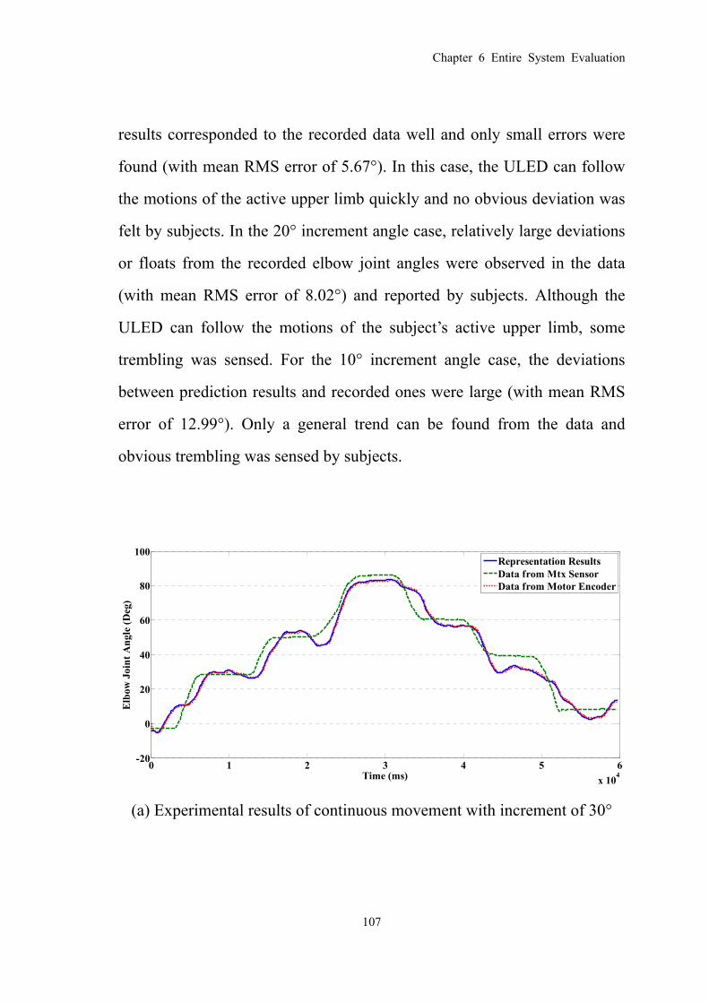
Chapter 6 Entire System Evaluation
107
results corresponded to the recorded data well and only small errors were
found (with mean RMS error of 5.67°). In this case, the ULED can follow
the motions of the active upper limb quickly and no obvious deviation was
felt by subjects. In the 20° increment angle case, relatively large deviations
or floats from the recorded elbow joint angles were observed in the data
(with mean RMS error of 8.02°) and reported by subjects. Although the
ULED can follow the motions of the subject’s active upper limb, some
trembling was sensed. For the 10° increment angle case, the deviations
between prediction results and recorded ones were large (with mean RMS
error of 12.99°). Only a general trend can be found from the data and
obvious trembling was sensed by subjects.
(a) Experimental results of continuous movement with increment of 30°
0 1 2 3 4 5 6x 10⁴
-20
0
20
40
60
80
100
Time (ms)
Elb
ow J
oint
Ang
le (D
eg)
Representation ResultsData from Mtx SensorData from Motor Encoder

Chapter 6 Entire System Evaluation
108
(b) Experimental results of continuous movement with increment of 20°
(c) Experimental results of continuous movement with increment of 10°
Figure. 6.8: Experimental results of consecutive stepping test
The evaluation experiment for self-training function shows that the
proposed method is able to provide a suitable prediction results for the
system to achieve the requirement of self-training at home. The method is
easy to calibrated and applied on other kind of purpose, e.g., intuitive
control of robot arm and human-machine interaction. It should be noticed
that the continuous prediction method has been applied on elbow joint up
0 1 2 3 4 5 6 7x 10⁴
0
20
40
60
80
100
Time (ms)
Elbo
w J
oint
Ang
le (D
eg)
Representation ResultsData from Mtx SensorData from Motor Encoder
0 1 2 3 4 5 6 7 8 9 10 11x 104
0
20
40
60
80
100
Time (ms)
Elb
ow J
oint
Ang
le (D
eg)
Representation ResultsData from Mtx SensorData from Motor Encoder

Chapter 6 Entire System Evaluation
109
to now, because elbow joint is relative simple compared with the other
joints of human body. With the increasing of DoFs, the dynamic function,
which is approximated to be a quadratic form between sEMG signals and
cosθ, may lost the straightforward expression form, especially when the
musculoskeletal system involved is redundancy.
6.4 Evaluation of remote force evaluation function
6.4.1 Schematic of remote force evaluation function
The remote force evaluation function aims to solve the problem that
the therapist is unable to evaluate the training effect of the patient except
patient goes to the rehabilitation center. The remote force evaluation
function will allow therapist to sense the contact force of the patient
remotely and give effective comments to the patient. Two issues involved
in this problem. The first one is the accuracy measurement of force value
and the second one is the representation of the force in a remote side. A
force sensor is a proper way for the first issue. However it is inconvenient
to attach force sensor on the surface in some cases or it may constraint the
movement of the patient. Another disadvantage to use the force sensor is
that it can only measure the output value of the entire musculoskeletal
system, not the performance of the individual muscles. We thus adopted
EMG to predict the contact force. For the second issue, a haptic device is a
suitable solution.
The schematic of the remote force evaluation function is depicted in
Fig. 6.9. Two motions, i.e., downward touch motion and push motion were
focused on to predict the contact force. Two musculoskeletal models with

Chapter 6 Entire System Evaluation
110
surface muscles involved were adopted for the two motions, respectively.
Dynamics equations for the two motions were developed based on the
musculoskeletal models. The equations were linear combination of
involved musculotendon forces. As the force exerting motion was isometric
in this study, a simplified Hill-type model was developed to calculate
musculotendon force for the individual muscle. In order to seek for the
proper parameters or weights involved in the dynamic equations, we
adopted the Bayesian linear regression (BLR). The off-line parameter
calibration was needed for BLR to compute the proper parameters. As the
whole movement of contact motion is complex, a motion recognition
method was used to classify the different motions. When force exerting
motion is detected, the well-calibrated dynamic equations will be used to
predict contact force. The predicted force is represented by haptic device
‘Phantom Premium’ on the remote side for the observer or therapist to
evaluate. The resolution of the ‘Phantom’ is good enough to mimic the
identical contact force.
Figure. 6.9: Schematic of proposed remote force evaluation method

Chapter 6 Entire System Evaluation
111
6.4.2 Experimental results
Five subjects (age: 26.00±1.73 years, height: 1.72±0.04 m, weight:
66.40±10.36 kg, all male, one left-handed, and four right-handed)
participated in the experiment. The pre-experimental process was similar
with the one which has been introduced in section 5.5.1. EMG signals were
recorded from the flexor carpi radialis (FCR), the flexor carpi ulnaris
(FCU), the extensor carpi radialis longus (ECRL), the extensor carpi
ulnaris (ECU), the extensor digitorum (ED), the biceps brachii (BB), the
triceps brachii (TB), and the pectoralis major (PM). One set of the
experimental results for downward touching force prediction were listed
from Table 6.2 to Table 6.4. The value is the RMS error between the
prediction result and recorded one.
Table 6.2 Force prediction for 5 N group with parameters calculated from 5 N group
Test Trails
Parameter Calibration Trials
5.1 5.2 5.3 5.4 5.5 5.6 5.7 5.8 5.9 5.10
5.1 0.05 1.29 1.24 3.82 3.34 5.64 1.68 8.36 2.35 3.44 5.2 1.02 0.04 0.93 2.58 2.38 4.00 2.30 6.52 2.37 7.65 5.3 1.27 1.38 0.21 4.56 1.74 4.35 2.99 7.22 1.31 6.62 5.4 2.76 1.92 1.72 0.51 1.87 2.40 2.35 4.65 1.80 3.80 5.5 2.23 1.12 0.91 3.13 0.39 1.93 2.57 4.57 1.11 5.07 5.6 3.60 2.54 1.65 3.74 1.12 0.67 2.81 2.23 1.92 5.37 5.7 3.64 1.69 1.38 3.42 2.68 3.32 0.41 6.09 1.44 7.09 5.8 6.28 4.28 3.00 3.41 2.07 2.63 2.86 0.79 2.72 6.15 5.9 2.84 1.86 1.25 3.50 2.10 3.52 1.71 6.05 1.20 3.00
5.10 3.04 3.00 2.29 3.47 2.76 4.51 2.45 6.08 2.40 0.58

Chapter 6 Entire System Evaluation
112
Table 6.3 Force prediction for 10 N group with parameters calculated from 5 N group
Test Trails
Parameter Calibration Trials
5.1 5.2 5.3 5.4 5.5 5.6 5.7 5.8 5.9 5.10
10.1 4.45 2.62 3.67 13.63 5.28 2.53 7.13 3.88 2.55 11.38 10.2 2.67 4.00 1.12 11.05 3.54 8.13 7.85 12.88 2.06 14.45 10.3 3.99 4.85 1.77 12.64 3.53 12.56 8.45 16.77 2.95 16.85 10.4 9.23 11.26 3.78 12.07 2.69 18.83 8.10 26.73 7.56 17.86 10.5 2.42 4.29 2.02 17.37 5.94 7.40 9.37 12.60 2.43 17.98 10.6 7.98 9.37 3.84 12.88 4.34 19.02 8.18 25.54 5.60 15.89 10.7 6.19 4.19 7.74 28.98 13.65 8.35 14.53 8.81 3.95 26.78 10.8 2.00 2.54 2.73 17.01 6.46 6.72 9.21 11.52 1.53 15.89 10.9 2.32 1.54 4.70 23.15 9.18 4.61 11.34 7.85 2.17 21.91
10.10 1.94 2.58 3.41 20.21 7.76 7.37 10.34 11.14 1.60 20.85
Table 6.4 Force prediction for 15 N group with parameters calculated from 5 N group
Test Trails
Parameter Calibration Trials
5.1 5.2 5.3 5.4 5.5 5.6 5.7 5.8 5.9 5.10
15.1 10.71 11.65 2.96 19.22 7.69 22.05 14.62 30.33 5.43 28.99 15.2 5.26 2.74 5.84 21.52 10.21 6.73 10.99 12.54 3.25 13.74 15.3 4.55 6.83 3.83 29.55 11.38 10.79 15.18 18.16 3.20 30.30 15.4 4.10 5.16 3.86 23.37 9.43 9.36 13.67 14.88 2.10 26.15 15.5 14.05 8.24 9.60 22.82 12.61 10.49 10.06 3.97 6.60 6.26 15.6 4.69 3.87 7.11 26.60 12.44 7.32 14.19 11.16 3.90 23.29 15.7 4.30 7.58 6.51 53.61 20.01 6.60 19.40 13.09 4.36 41.75 15.8 3.66 4.17 7.18 37.78 15.79 4.57 17.06 9.86 2.93 33.43 15.9 1.72 0.46 0.88 11.37 2.68 2.37 2.76 0.48 1.14 7.78
15.10 3.98 7.14 3.54 30.43 12.02 9.54 13.46 17.76 3.77 23.59
The subtitle in the three tables is with the form of m.n where m
denotes the force group and n denotes the n trial in this group. It can be
indicated that as the parameters were calibrated by 5 N group, the RMS
values in diagonal elements of Table 6.2 is the smallest. BLR can guarantee

Chapter 6 Entire System Evaluation
113
to find the optimal parameters in one special data space. However, the
time-variable property of EMG signals makes it difficult or impossible to
acquire a special data space which is sufficient to represent the entire data
space. This kind of property can be indicated from the other groups. Some
of the RMS errors from the other groups are quite large.
Given these situations, two questions come naturally. The first one is
whether the different groups share the same data space. And the second one
is that how long it takes to find the property parameters. The first question
is essential. As shown in section 5.5.3 that, there is a constant ‘pattern’ in
the trend of muscle activation levels of individual involved muscles during
the contact force exerting motion. The linearity of these muscles is different.
In other research results [101-103], the relation between muscle activation
level and the musculotendon force was also studied and it is certainly not
‘random’. It is also reasonable that the ‘commands’ sent by the CNS are
some fixed ‘patterns’. These patterns reflect certainly in the EMG signals
as EMG signals are the electrical representation of the CNS commands. For
the second problem, it will take only one time calibration to find the proper
parameters if a suitable data space can be obtained. Actually, it is extremely
luck to acquire such kind of data space at the first time. In the given
situation, we tested 10 trials for each group and conducted the
‘cross-validation’ on the total 30 sets of data. Table 6.2 to 6.4 listed the
results of calibration with 5 N group and tests on the whole data. The other
cases are listed from Table 6.5 to 6.10. The optimal parameters are marked
as red for each group. It can be indicated that the optimal ones for one

Chapter 6 Entire System Evaluation
114
group are also the optimal ones for the other group. This case happens on
the other subjects as well. With the help of computer, it takes not much
time to cross-validate the results on the whole 30 sets of data. However it
really takes time for the subject to perform 30 times of tests. In this case we
suggest that 10 times of tests for one group are performed and then use
cross-validation to find the optimal parameters. Another two tests of the
other two groups, respectively, are then conducted to test the optimal
parameters.
Table 6.5 Force prediction for 5 N group with parameters calculated from 10 N group
Test Trails
Parameter Calibration Trials
10.1 10.2 10.3 10.4 10.5 10.6 10.7 10.8 10.9 10.10
5.1 4.50 2.81 0.73 2.06 3.61 4.24 6.02 4.22 4.09 2.75 5.2 3.80 2.69 1.02 2.25 3.50 4.80 5.96 4.24 3.90 3.55 5.3 3.35 1.34 0.93 2.89 2.01 2.45 5.43 2.67 2.93 2.55 5.4 2.04 1.97 2.25 4.01 2.11 2.77 4.36 2.20 2.59 3.60 5.5 1.95 0.85 1.68 3.80 1.07 1.64 5.16 1.62 1.46 2.84 5.6 1.23 1.50 2.46 4.49 1.50 2.12 4.41 1.59 2.39 3.91 5.7 3.13 1.96 2.15 6.00 2.30 2.66 8.91 2.67 3.07 5.64 5.8 1.33 2.36 3.99 7.47 2.16 2.18 5.61 1.72 4.28 6.81 5.9 2.55 1.35 2.08 4.82 1.56 1.92 5.90 1.98 1.81 3.73
5.10 3.21 2.53 2.51 4.41 2.73 2.75 4.25 2.74 3.33 3.36

Chapter 6 Entire System Evaluation
115
Table 6.6 Force prediction for 10 N group with parameters calculated from 10 N group
Test Trails
Parameter Calibration Trials
10.1 10.2 10.3 10.4 10.5 10.6 10.7 10.8 10.9 10.10
10.1 0.54 2.62 4.02 7.17 2.30 3.33 5.06 1.91 3.23 5.91 10.2 4.84 0.61 1.04 3.25 0.98 2.22 4.72 1.43 4.47 2.15 10.3 6.71 1.81 0.91 2.35 2.38 1.74 4.66 2.33 6.31 3.45 10.4 12.51 4.23 3.39 0.97 5.20 1.94 10.33 5.76 11.97 7.67 10.5 4.79 1.20 1.69 4.42 0.96 2.96 6.24 1.20 3.78 1.91 10.6 11.45 4.08 2.59 2.33 4.90 0.86 8.35 4.70 9.89 5.82 10.7 4.72 7.39 6.55 8.93 7.35 7.55 1.92 6.31 5.35 6.63 10.8 3.88 1.91 2.46 5.81 1.40 2.88 6.22 0.75 2.11 2.46 10.9 2.03 3.82 3.72 6.08 3.34 3.84 3.18 2.53 1.06 2.76
10.10 3.71 2.71 2.56 4.40 2.29 3.11 3.56 1.72 2.76 1.35
Table 6.7 Force prediction for 10 N group with parameters calculated from 15 N group
Test Trails
Parameter Calibration Trials
10.1 10.2 10.3 10.4 10.5 10.6 10.7 10.8 10.9 10.10
15.1 12.23 3.06 2.43 2.47 3.91 4.35 4.37 3.45 12.63 8.61 15.2 4.45 5.30 5.95 12.08 4.80 5.91 10.31 3.59 3.61 8.45 15.3 6.70 3.01 2.42 5.75 2.33 5.11 6.18 1.68 5.43 2.39 15.4 4.94 2.95 2.88 5.37 2.23 4.92 3.39 1.61 4.45 3.16 15.5 5.19 9.37 10.64 19.05 9.12 8.72 11.30 6.80 12.80 18.52 15.6 4.41 6.48 6.30 9.97 6.02 6.97 4.75 4.99 3.86 6.01 15.7 5.40 5.93 3.92 9.39 5.57 6.78 11.57 3.63 4.25 4.40 15.8 3.22 6.50 5.42 8.90 6.06 7.51 4.65 4.88 3.14 4.56 15.9 0.30 0.16 0.40 1.99 0.07 1.39 4.58 0.96 0.45 1.26
15.10 7.16 3.07 2.66 8.61 2.54 5.30 11.43 1.76 4.49 3.79

Chapter 6 Entire System Evaluation
116
Table 6.8 Force prediction for 5 N group with parameters calculated from 15 N group
Test Trails
Parameter Calibration Trials
15.1 15.2 15.3 15.4 15.5 15.6 15.7 15.8 15.9 15.10
5.1 6.78 7.24 3.28 6.64 7.07 3.37 1.92 2.24 16.21 3.26 5.2 7.31 7.24 3.56 6.64 6.46 3.39 1.68 2.39 11.33 3.49 5.3 6.13 5.32 2.16 4.94 5.46 3.04 2.57 2.36 14.82 2.04 5.4 5.81 3.92 2.71 4.13 4.80 1.94 1.68 1.47 9.62 1.83 5.5 4.73 3.36 1.58 3.72 4.29 2.67 1.61 1.70 7.48 1.64 5.6 5.33 2.39 2.45 2.99 3.44 2.06 1.69 1.67 7.36 1.59 5.7 8.98 4.00 2.83 5.91 7.81 5.46 2.19 3.19 13.12 3.14 5.8 8.00 2.10 3.79 1.91 3.09 2.78 2.00 1.87 5.46 1.63 5.9 6.44 3.68 2.01 4.60 6.13 3.29 2.29 2.31 14.30 1.95
5.10 5.43 4.20 2.85 3.88 5.03 1.86 2.19 1.83 12.44 2.11
Table 6.9 Force prediction for 10 N group with parameters calculated from 15 N group
Test Trails
Parameter Calibration Trials
15.1 15.2 15.3 15.4 15.5 15.6 15.7 15.8 15.9 15.10
10.1 9.23 2.01 3.90 1.61 2.45 2.63 3.86 2.79 11.37 2.30 10.2 3.62 5.43 1.43 3.02 3.42 1.95 4.26 1.74 26.97 1.56 10.3 2.97 6.88 2.48 3.79 6.05 1.65 4.76 1.74 27.08 1.40 10.4 3.09 11.99 6.09 7.59 9.01 5.74 2.87 5.11 51.65 3.44 10.5 5.55 4.83 1.36 2.64 3.24 3.01 4.23 2.39 30.99 1.86 10.6 2.95 9.67 4.36 6.58 9.54 4.18 4.03 3.47 44.55 2.16 10.7 9.70 5.76 6.36 6.33 7.78 3.21 6.68 4.12 20.10 5.14 10.8 6.49 3.29 1.59 2.06 3.69 2.64 3.98 1.82 26.08 1.50 10.9 6.10 1.26 2.61 2.14 3.59 2.72 5.05 3.04 17.94 3.12
10.10 3.94 3.07 1.46 1.75 3.09 2.00 4.64 2.44 21.77 2.42

Chapter 6 Entire System Evaluation
117
Table 6.10 Force prediction for 15 N group with parameters calculated from 15 N group
Test Trails
Parameter Calibration Trials
15.1 15.2 15.3 15.4 15.5 15.6 15.7 15.8 15.9 15.10
15.1 1.60 10.40 4.67 4.39 6.44 2.52 8.67 2.30 57.95 3.16 15.2 15.96 2.20 5.75 2.92 6.16 5.37 4.14 3.39 35.60 3.33 15.3 6.41 4.81 1.60 1.96 3.29 2.53 5.85 2.20 46.72 2.95 15.4 5.24 3.84 1.73 0.97 1.96 2.58 6.71 2.63 37.03 3.34 15.5 25.24 8.39 12.09 3.11 1.80 5.92 2.36 2.85 23.56 3.22 15.6 10.84 3.43 5.52 4.01 4.66 3.15 6.13 3.72 29.53 4.93 15.7 12.57 3.55 3.96 3.11 5.40 6.32 1.74 5.81 60.40 2.35 15.8 10.05 3.09 4.86 4.24 5.64 2.67 5.34 2.73 39.47 4.73 15.9 1.03 1.50 0.33 1.94 1.09 3.11 2.17 2.63 0.02 1.86
15.10 12.29 4.32 2.57 2.73 4.33 6.15 2.41 4.75 55.58 1.48
The relative RMS errors for the five subjects are within 20% and this
error exists in the entire tests data, i.e., it is more like a constant value
rather than an average one. As some muscles involved are at the deep layer,
it is impossible to record the accuracy EMG signals from these muscles.
The constant 20% errors may be caused by the undetected muscles.
Another reason may be given rise to the muscular model. Although
Hill-type model is a classic and conventional model for muscle, it is not
accuracy enough. On the other hand, many approximations were assumed
during the dynamic equation development. All of these bring uncertainty to
the results and cause the constant 20% error.
Another important issue is the adoption of proportion smooth
algorithm (5-12) which is used to address the problem of force impact
caused by the resolution of motion recognition classifier. The resolution of
Chapter 6 Entire System Evaluation
118
the classifier defined in this thesis is the time delay between a motion
sensor (MTx sensor) detected starting point and the classifier detected
starting point for a special movement. According to the experimental
results of motion recognition, the resolution is about 100-200ms. That is to
say the classifier cannot detect the motion as soon as it happens. However
the EMG signals go on as well. This give rise to one problem that when
classifier detects the motion and then informs the controller to calculate the
contact force, the force is already so high that it is not continuous from the
previous time point. That is the reason for the force impact on the remote
side. The proportion smooth algorithm increases the force generation time
manually with the trade-off of accuracy. As the algorithm only spreads the
‘impact’ within 100ms, the trade-off is acceptable and the effort of
eliminating the impact feeling is helpful for mimicking the original contact
force.
The experimental results prove the efficiency of the proposed remote
force evaluation function for our rehabilitation system, which will help the
therapist to supervise the patient more efficiently.
6.5 Summary
In this chapter, the evaluation for the entire system was conducted.
Testing experiments were performed for self-training function and remote
force evaluation function. The experimental results coincided with the
simulation results in the corresponded chapter, respectively. The
self-training function, which was achieved by extraction of reference
command signals from EMG signals of the intact arm for the ULERD worn

Chapter 6 Entire System Evaluation
119
on the impaired arm, provided a bilateral rehabilitation training function
allowed patient to perform the training exercise under the willing of their
own without the supervision of therapist. The prediction results with RMS
lower than 10° show that the proposed method can provide suitable control
effect for the self-training purpose. The remote force evaluation function,
which was achieved by using only EMG signals, allows the therapist to
evaluate the training effect remotely. This will benefit both the therapists
and patients.
Additionally, some issues involved in these methods were also
discussed in order to address the problems more clearly and provide some
ideas for the similar problems.

Chapter 6 Entire System Evaluation
120

Chapter 7 Concluding Remarks
121
Chapter 7 Concluding Remarks
7.1 Thesis summary
Stroke is the second leading cause of disability, which wildly affects
peoples’ Activities of Daily Living (ADL) and the life style of their families.
The tremendous contradiction is the large demand for special clinical care
and the limited number of therapists. The purpose of the proposed system is
to provide home-used self-training rehabilitation for stroke patients.
Our previous developed Upper-limb Exoskeleton Rehabilitation
Device (ULERD) was designed to be portable to guarantee the capability to
be used at home. The ‘self-training’ property was achieved by the proposed
bilateral training method, in which the impaired arm was carried by
ULERD and the control signals were extracted from the EMG signal from
the intact arm. The proposed system also provides remote force evaluation
function for therapist to evaluate the training effect of the patient remotely.
This function allows the therapist supervises and gives suggestion to
patient efficiently, without meeting the patient face to face.
To accurately extract motion information from sEMG signals, we first
adopted a motion recognition based method. The Autoregressive (AR)
model was applied to extract the features from the sEMG signals and a
Neural Network (NN) classifier was trained to recognize the motions. The
parameters involved in the AR model were decided by AIC criterion and
the recognition results were processed by an experiential method to acquire

Chapter 7 Concluding Remarks
122
the final control command to the ULERD. As the recognition accuracy rate
was not good enough and the results were unstable, a Hill-type muscular
model based feature extraction method and a Support Vector Machine
(SVM) was applied to improve the recognition results. The recognition
accuracy rate increased from 85% to 96%.
In order to address the drawback of the motion recognition based
method that it can only provide binary-like control reference to the device,
a continuous elbow joint angle prediction method was proposed. In this
method, a quantitative relation between sEMG signals and elbow joint
angle was developed based on the Hill-type based muscular model and our
proposed simplified musculoskeletal model of elbow joint in sagittal plane.
After some approximation, a quadratic-like equation was found and
validated by a four-day experiment on ten subjects. Furthermore, a state
switch model was developed to solve the problem of time-variable of
sEMG signals. The experimental results showed that the proposed method
can provide a prediction results with RMS errors below 10°.
For the purpose of remote force evaluation, a force prediction method
using only sEMG signals was designed. As the complex of musculoskeletal
structure, isometric downward touch motion and push motion were focused
on in this study. Two musculoskeletal models were used to represent the
two motions, respectively. The dynamic equations were yielded based on
the combination of Hill-type based muscular model and the proposed
musculoskeletal models. The motions were recognized by a NN classifier
and the desired forces were calculated by the dynamic equations when the

Chapter 7 Concluding Remarks
123
force exerting motion was detected. The force representation was achieved
by a haptic device ‘Phantom Premium’ which is a high fidelity device for
sensation generation. The experimental results show that the proposed
method can predict the contact force with relative RMS errors within 20%.
The entire system was evaluated for the self-training function and
remote force evaluation function, respectively, at the last of this thesis. The
experimental results indicated that the self-training function supported by
the proposed continuous elbow joint angle prediction method is suitable to
allow patients to perform the rehabilitation training by themselves. The
remote force evaluation function is also sufficient to allow the therapist to
evaluate the training effect of the patient.
7.2 Research achievement
(1) Design of the bilateral rehabilitation training based on EMG signals.
The proposed bilateral rehabilitation training aims to allow patient to
train his/her impaired arm with the intact arm. In this training, patient
performs bilateral movement with both of the arms. The impaired arm
wears our developed ULERD under the direction of the intact arm to
complete the same movement. In this way, the patients can complete the
training exercise by themselves under the wills of their own. The new point
here is that we extract the control signals from the sEMG signals which
reflect the intention of patients, not just movement. From the
neurorehabilitation point of view that the training effort will be better if the
motion is inspired by neuro system, not just passive motion following. The
system, with our proposed method, can help patients to move their

Chapter 7 Concluding Remarks
124
impaired arms under the control of the neuro system, i.e., by the control
command from the EMG signals.
(2) Development of continuous elbow joint angle prediction method using
only sEMG signals.
The proposed method aims to address the drawback of the motion
recognition method that it can only provide binary-like reference control
signals. Pattern recognition based methods have been studied widely
around the world. However, the continuous prediction type is seldom
proposed. In this study, we combined the Hill-type based muscular model
and a simplified elbow joint musculoskeletal model to yield the mathematic
expression between sEMG signals recorded from Biceps Brachii and the
elbow joint angle. As many parameters involved in the Hill-type based
muscular model, some approximations were assumed for simplification.
The modified dynamic equation released quadratic-like relation between
muscle activation level, which can be calculated from sEMG signals, and
the cosθ. Although the situation of elbow joint is relative simple compared
with the other joints, this kind of method introduces an alternative way to
use EMG signals to predict motions or joint angles.
(3) Force prediction using only EMG signals.
The relationships between musclotendon force and EMG signals have
been widely studied. However, seldom focus has been paid on using EMG
signals to predict the contact force between human and environment.
Although the EMG signal is heavily unstable and time-variable, it has
potential to represent the individual muscle status and predict the contact

Chapter 7 Concluding Remarks
125
force even it is very hard to attach force sensor on the contact surface. In
order to avoid the complex of redundancy of musculoskeletal structure, a
motion recognition method was adopted to classify the different force
exerting motions and the period of force exerting. This method combined
with a haptic device can form a remote force evaluation system. This kind
of system also can mimic the true contact motion between human and
human in virtual-reality.
(4) Found of relation between motion recognition and different
classification method.
We compared different classification method and feature extraction
method to find the relation between them. The experimental results
indicated that using the feature processed with a low-pass filter with cut-off
frequency with 4 to 10 Hz will make the recognition better than direct
using the feature extraction results for classifier training. Furthermore, it is
found that the Support Vector Machine (SVM) performs better than Neural
Network (NN) in real-time test, while the time consumption is much higher
than NN. The reason is that SVM uses massive support vectors to represent
the boundary for different motions while the number of parameters
involved in NN is constant. Using the low-pass filter processing will reduce
the support vectors as well.
7.3 Recommendations for the future
Motion recognition using EMG signals is a compelling topic which
will bring benefit to many application fields. However, seldom applies have
been sighted outside laboratory environment. The non-stationary,

Chapter 7 Concluding Remarks
126
time-variable and easily affected properties are the primary reasons that
prevent the application. Feature extraction plays an important role in this
issue. The ideal feature extraction method is the one that can avoid the
effect by the external factors and extract the expected features ignoring the
non-stationary and time-variable. On the other hand, the concept of muscle
synergy could be used for this issue. The muscle synergy releases the
relation between EMG signals changing and the command trend from the
CNS. There are some constant behavers in the muscle synergy for the same
motions. Up to now, only downward touch motion and push motion have
been studied. Other types of motions are recommended, such as poll
motion and the gait motion. In gait motion, this kind of method may be
used to predict the interaction force from the ground.
For the home-used rehabilitation system, a human-like arm for the
therapist side is recommended. Actually, a very simple prototype is being
designed in our group. This kind of device will be designed to own the
ability to mimic the status of real human arm, which will help the therapist
more to estimate the rehabilitation effort of the patient.
References
127
References
[1]. http://www.world-heart-federation.org/cardiovascular-health/stroke/
[2]. J. H. Carr, R. B. Shepherd, editors. Movement Science: Foundations
for Physical Therapy in Rehabilitation. Rockville, MD:Aspen; 1987.
[3]. J. A. Kleim, E. Lussnig, E. R. Schwarz, T. A. Comery and W. T.
Greenough. Synaptogenesis and FOS expession in the motor cortex
of the adult rat after motor skill learning, J. Neurosci, Vol.16,
pp.4529-4535, 1996.
[4]. F. W. George, R. Chen, K. Ishii, K. Obushara, S. Eckloff, E. Croarkin,
E. Taub, L. H. Gerber, M. Hallett and L. G. Cohen.
Constraint-induced therapy in stroke: Magnetic-stimulation motor
maps and cerebral activation, Neurorehabl. Neural Repair., Vol.17,
pp.48-57, 2003.
[5]. B. H. Dobkin, D. Apple, H. Barbeau, M. Basso, A. Behrman, D.
Deforge, J. Ditunno, G. Dudley, R. Elashoff, L. Fugate, S. Harkema,
M. Saulino and M. Scott. Methods for a randomized trial of
weight-supported treadmill training versus conventional training for
walking during inpatient rehabilitation after incomplete traumatic
spinal cord injury, Neurorehabil. Neural Repair, Vol.17, pp.152-67,
2003.
[6]. S. J. Page. Intensity versus task-specifity after stroke: how important
is intensity? Am J. Phys Med Rehabi., Vol. 82, pp.730-732, 2003
[7]. J. Furusho, K. Koyanagi, Y. Imada, Y. Fujii, et al. A 3-D

References
128
rehabilitation system for upper limbs developed in a 5-year NEDO
project and its clinical testing. Proceedings of the 2005 IEEE 9th
International Conference on Rehabilitaiton Robotics, pp.53-56. 2005.
[8]. P. S. Lum, C. G. Burgar, M. V. Loos, et al. MIME robotic device for
upper-limb neurorehabilitation in subacute stroke subjects: A
follow-up study. J. Rehabil. Res. Dev., Vol. 43, pp 631-642, 2006.
[9]. R. E. Schleenbaker, and A. G. Mainous. Electromyographical
biofeedback for neuromuscular re-education in the hemiplegic stroke
patient: a meta-analysis, Arch. Phys. Med. Rehabil., 74, pp.
1301-1304, 1993.
[10]. L. SONDE, C. Gip, S. E. Fernaeus, C. G. Nilsson, and M. Vitanen.
Stimulation with low frequency (1.7Hz) transcutaneous electric nerve
stimulation (low-tens) increases motor function of the post-stroke
paretic arm, J. Rehabil. Med., Vol. 30, pp. 95-99, 1998.
[11]. J. W. Krakauer. Motor learning: its relevance to stroke recovery and
neurorehabilitation. Current opinion in neurology, Vol. 19, pp 84-90,
2006.
[12]. G. Kwakkel, B. J. Kollen, and R. C. Wagenaar. Long term effects of
upper and lower limb training after stroke: a randomised trial, J.
Neurol. Neurosurg. Psychiat., Vol. 72, pp. 473-479, 2002.
[13]. H. Kwee, J. Duimel , J. Smit, A. T. Mold, J. Woerden, and L. V. D.
Kolk. The manus wheelchair-mounted manipulator: developments
toward a production model. Proc. 3rd Int. Conf. Assoc. Advancement
Rehab. Technol., pp. 460-462, 1988.

References
129
[14]. L. Leifer. Rehabilitive robotics, Robot Age, pp. 4-11, 1981.
[15]. V. D. Loos, H. F. M. Michalowski, and J. L. Leifer. Development of
an omnidirectional mobile vocational assistant robot. Proc. 3rd Int.
Conf. Assoc. Advancement Rehab. Technol., pp. 468-469, 1988.
[16]. N. Hogan, H. I. Krebs, A. Sharon, and J. Charnnarong. Interactive
robotic therapist. U.S. Patent, 5466213, 1995.
[17]. H. I. Krebs, N. Hogan, M. L. Aisen, and B. T. Volpe. Robot-aided
neurorehabilitation, IEEE Trans. Rehab. Eng., Vol. 6, pp. 75-87,
1998.
[18]. T. Nef, R. Riener. ARMin – design of a novel arm rehabilitation robot.
Proceedings of the 2005 IEEE 9th International Conference on
Rehabilitation Robotics, pp. 57-60, 2005.
[19]. T. Nef, M. Mihelj, R. Riener. ARMin: a robot for patient-cooperative
arm therapy. Med. Bio. Eng. Comput., Vol. 45, pp. 887-900, 2007.
[20]. P. S. Lum, C. G. Burgar, V. Loos, P. C. Shor, M. Majmundar, R. Yap.
The MIME robotic system for upper-limb neuro-rehabilitation:
results from a clinical trial in subacute stroke. Proceedings of the
2005 IEEE 9th International Conference on Rehabilitation Robotics,
pp. 511-514, 2005.
[21]. C. Beurskens, P. Heymans. Mime therapy improves facial symmetry
in people with long-term facial nerve paresis: A randomised
controlled trial. Aust, J. Physiother., Vol. 52, pp. 177-183, 2006.
[22]. R. Riener, T. Nef, G. Colombo. Robot-aided neurorehabilitation of
the upper extremities. Med. Biol. Eng. Comput., Vol 43, pp. 2-10,

References
130
2005.
[23]. M. Zinn, B. Roth, O. Khatib, and J. K. Salisbury. A new actuation
approach for human friendly robot design, Int. J. Robot. Res., Vol. 23,
pp. 379-398, 2004.
[24]. N. Hogan. Impedance control: An approach to manipulation: Part II –
Implementation. J. Dyn. Sys., Meas., Control., Vol 107, pp. 17-24,
1985.
[25]. V. G. Popescu, G. C. Burdea, M. Bouzit, V. R. Hentz. A
virtual-reality-based telerehabilitation system with force feedback.
IEEE T. Inf. Technol. B., Vol. 4, pp. 45-51, 2000.
[26]. D. Jack, R. Boian, A. S. Merians, M. Tremaine, G. C. Burdea, S. V.
Adamovich, M. Recce, H. Poizner. Virtual reality-enhanced stroke
rehabilitation. IEEE T. Neur. Sys. Reh., Vol. 9, pp. 308-318, 2001.
[27]. A. Henderson, N. Korner-Bitensky, M. Levin. Virtual reality in stroke
rehabilitation: A systematic review of its effectiveness for upper limb
motor recovery. Top. Stroke. Rehabil., Vol. 14, pp. 52-61, 2007.
[28]. C. J. Luca. The Use of Surface Electromyography in Biomechanics, J.
of Appl. Biomech., Vol.13, pp. 1-38, 1997.
[29]. D. Stashuk, EMG signal decomposition: how can it be accomplished
and used, J. Electromyogr. Kines., Vol.11, pp. 151-173, 2001.
[30]. T. S. Buchanan, D. G. Lloyd, K. Manal and T. F. Besier.
Neuromusculoskeletal modeling: estimation of muscle forces and
joint moments and movements from measurements of neural
command, J. Appl. Biomech., Vol. 20, pp. 367-395, 2004.

References
131
[31]. D. G. Lloyd, T. F. Besier. An EMG-driven musculoskeletal model for
estimation of the human knee joint moments across varied tasks. J.
Biomech., Vol. 36, pp. 765-776, 2003.
[32]. D. G. Lloyd, T. S. Buchanan. A model of load sharing between
muscles and soft tissues at the human knee during static tasks.
Journal of Biomechanical Engineering, Vol. 118, pp. 367-376, 1996.
[33]. K. Manal, R. V. Gonzalez, D. G. Lloyd, T. S. Buchanan. A real-time
EMG driven virtual arm. Comput. Biol. Med., Vol. 32, pp. 25-36,
2002.
[34]. O. Fukuda, T. Tsuji and A. Otsuka. A human-assisting manipulator
teleoperated by EMG signals and arm motions, IEEE T. Robot.
Autom., Vol. 19, pp. 210-222, 2003.
[35]. M. V. Liarokapis, P. K. Artemiadis, P. T. Katsiaris, K. J.
Kyriakopoulos and E. S. Manolakos. Learning human reach-to-grasp
strategies: towards EMG-based control of robotic arm-hand systems,
Proc. IEEE Int. Conf. Robot., 2287-2292, 2012.
[36]. P. K. Artemiadis and K. J. Kyriakopoulos, A switching regime model
for the EMG-based control of a robot arm, IEEE T. Syst. Man CY. B.,
41: 53-63, 2009.
[37]. Z. Ju, G. Ouyang, M. Wilamowska-Korsak, et al. Surface EMG
Based Hand Manipulation Identification Via Nonlinear Feature
Extraction and Classification. IEEE SENSORS JOURNAL, Vol 13,
pp 3302-3311, 2013.
[38]. A. F. Huxley. Muscle structure and theories of contraction. Progr.

References
132
Biophys. Biophys. Chem., Vol. 7, pp. 255-318, 1958.
[39]. A. F. Huxley and R. M. Simmons. Proposed mechanism of force
generation in striated muscle. Nature, Vol. 233, pp. 533-538, 1971.
[40]. A. V. Hill. The heat of shortening and the dynamic constants of
muscle. Proc. Roy. Soc. Lond. B. Biol. Sci., Vol. 126, pp. 136-195,
1938.
[41]. E. Cavallaro, J. Rosen, J. C. Perry, S. Burns and B. Hannaford.
Hill-based model as a myoprocessor for a neural controlled powered
exoskeleton arm -parameters optimization. Proc. IEEE Int. Conf.
Robotics & Automation, 4525-4530, 2005.
[42]. K. Manal, R. V. Gonzalez, D. G. Lloyd and T. S. Buchanan. A
real-time EMG-driven virtual arm. Comput. Biol. Med., Vol. 32, pp.
25-36, 2002.
[43]. C. Fleischer, G. Hommel. A Human–Exoskeleton Interface Utilizing
Electromyography. IEEE T. Robot., Vol. 24, pp. 872-882, 2008.
[44]. T. Lenzi, S. M. M. Rossi, N. Vitiello, et al. Intention-Based EMG
Control for Powered Exoskeletons. IEEE T. BIO-MED. ENG., Vol.
59, pp. 2180-2190, 2012.
[45]. S. Kwon, Y. Kim, J. Kim. Movement Stability Analysis of Surface
Electromyography-Based Elbow Power Assistance. IEEE T.
BIO-MED. ENG., Vol. 61, pp. 1134-1142, 2014.
[46]. A. Ajoudani, N. Tsagarakis, A. Bicchi. Tele-impedance:
Teleoperation with impedance regulation using a body–machine
interface. Int. J. Robot. Res., Vol. 31, pp. 1642-1655, 2012.

References
133
[47]. X. Chen and Z. J. Wang. Pattern recognition of number gestures
based on a wireless surface EMG system. Biomed. Signal. Proces.,
Vol. 8, pp. 184-192, 2013.
[48]. X. Tang, Y. Liu, C. Lv and D. Sun. Hand motion classification using
a multi-channel surface electromyography sensor. Sensors, Vol. 12,
pp. 1130-1147, 2012.
[49]. A. Phinyomark, F. Quaine, S. Charbonnier, C. Serviere, F.
Tarpin-Bernard and Y. Laurillau. A feasibility study on the use of
anthropometric variables to make muscle-computer interface more
practical. Eng. Appl. Artif. Intell., Vol. 27, pp. 1681-1688, 2013.
[50]. L. Lucas, M. DiCicco, and Y. Matsuoka. An EMG-controlled hand
exoskeleton for natural pinching. J. Robot. Mechatron., Vol. 16, pp.
482-488, 2004.
[51]. P. Wojtczak, T. G. Amaral, O. P. Dias, A. Wolczowski and M.
Kurzynski. Hand movement recognition based on biosignal analysis.
Eng. Appl. Artif. Intell., Vol. 22, pp. 608-615, 2008.
[52]. N. Bu, M. Okamoto and T. Tsuji. A hybrid motion classification
approach for EMG-based human-robot interfaces using bayesian and
neural networks. IEEE T. Robot., Vol. 25, pp. 502-511, 2009.
[53]. E. A. Clancy, and N. Hogan. Single site electromyograph amplitude
estimation. IEEE T. Bio-Med. Eng., Vol. 41, pp. 159-167, 1994
[54]. E. A. Clancy. Electromyogram amplitude estimation with adaptive
smoothing window length. IEEE T. Bio-Med. Eng., Vol. 46, pp.
717-729, 1999.

References
134
[55]. C. J. Luca, L. D. Gilmore, M. Kuznetsov, et al. Filtering the surface
EMG signal: Movement artifact and baseline noise contamination. J.
Biomech., Vol. 43, pp. 1573-1579, 2010.
[56]. Z. Song, S. Guo, Y. Fu. Development of an upper extremity motor
function rehabilitation system and an assessment system. Int. J.
Mechatronics and Automation, Vol 1, pp. 19-28, 2011.
[57]. Z. Song, S. Guo. Development of a new compliant exoskeleton
device for elbow joint rehabilitation. Proceeding of the 2011
IEEE/ICME International Conference on Complex Medical
Engineering, pp. 647-654, 2011.
[58]. Z. Song, S. Guo, N. Xiao, L. Shi, B. Gao. Implementation of
human-machine synchronization control for active rehabilitation
using an inertia sensor, Sensors, Vol. 12, pp. 16046-16059, 2012.
[59]. Z. Song, S. Guo. Study on impedance generation using an
exoskeleton device for upper-limb rehabilitation, Proceedings of
2012 IEEE International Conference on Multisensor Fusion and
Integration for Intelligent Systems, pp. 281-286, 2012.
[60]. C. Cipriani, C. Antfolk, C. Balkenius, B. Rosén, G. Lundborg, M.
Carrozza, and F. Sebelius. A novel concept for a prosthetic hand with
a bidirectional interface: A feasibility study,” IEEE Trans. Biomed.
Eng., vol. 56, no. 11, pp. 2739-2743, Nov. 2009.
[61]. A. Arieta, H. Yokoi, T. Arai, and W. Yu. Study on the effects of
electrical stimulation on the pattern recognition for an EMG
prosthetic application. Proc. IEEE Int. Conf. Eng. Med. Biol. Soc., pp.

References
135
6919-6922, 2006.
[62]. D. Zhang, X. Chen, S. Li, P. Hu, and X. Zhu. EMG controlled
multifunctional prosthetic hand: Preliminary clinical study and
experimental demonstration. Proc. IEEE Int. Conf. Robot. Autom., pp.
4670-4675, 2011.
[63]. P. R. Cavanagh, P. V. Komi. Electromechanical delay in human
skeletal muscle under concentric and eccentric contractions. Eur. J.
Appl. Physiol. Vol. 42, pp. 159-163, 1979.
[64]. M. B. I. Reaz, M. S. Hussain, and F. Mohd-Yasin. Techniques of
EMG signal analysis: detection, processing, classification and
applications. Biomedical and Life Sciences, Vol. 8, pp. 11-35, 2006.
[65]. M. Pang, S. Guo, and Z. Song. Study on the sEMG driven upper limb
exoskeleton rehabilitation device in bilateral rehabilitation. Journal
of Robotics and Mechatronics, Vol. 24, No. 4, pp. 585-594, 2012.
[66]. W. S. McCulloch, W. Pitts. A logical calculus of the ideas immanent
in nervous activity. B. Math. Biophys., Vol. 5, pp. 115-133, 1943.
[67]. B. Widrow, M. E. Hoff. Adaptive switching circuits. Ire Wescon
Convention record, Vol. 4, pp. 96-104, 1960.
[68]. C. V. Malsburg. F. Rosenblatt: Principles of neuraldynamics:
perceptrons and the theory of brain mechanisms. Brain Theory, pp.
245-248, 1986.
[69]. A. M. Chen, H. Lu, R. Hecht-Nielsen. On the geometry of
feedforward neural network error surfaces. Neural. Comput., Vol. 5,
pp. 910-927, 1993.

References
136
[70]. SENIAM project. [http://www.seniam.org/]
[71]. H. L. Lew, S. J. Tsai. Johnson’s practical electromyography. 4th ed.
Philadelphia: Lippincott Williams & Wilkins, 2007.
[72]. C. Cortes, V. Vapnik. Support-Vector Networks. Machine Learning,
20(3): 273-297, 1995.
[73]. J. C. Platt. Fast training of support vector machines using sequential
minimal optimization. In B. Scholkopf, C. J. C. Burges, and A. J.
Smola, Advances in kernel methods - Support Vector Learning, pp.
185-208. MIT press.
[74]. Z. Song, S. Guo, M. Pang, S. Zhang. Study on Recognition of Upper
Limb Motion Pattern Using surface EMG signals for Bilateral
Rehabilitation, Proceedings of 23rd 2012 International Symposium
on Micro-NanoMechatronics and Human Science, pp. 425-430,
2012.
[75]. http://en.wikipedia.org/wiki/File:Hill_muscle_model.svg.
[76]. M. Pang, S. Guo, Q. Huang, H. Ishihara, H. Hirata. An EMG-based
Quantitative Representation Method for the Upper Limb Elbow Joint
Angle in Sagittal Plane. J. Med. Biol. Eng, doi:10.5405/jmbe.1843,
2014.
[77]. M. Pang, S. Guo, Z. Song and S. Zhang. A Surface EMG
Signals-based Real-time Continuous Recognition for the Upper Limb
Multi-motion. Proceedings of 2012 IEEE International Conference
on Mechatronics and Automation, pp.1984-1989, 2012.
[78]. S. M. Kay. Modern spectral estimation: Theory and application.

References
137
Englewood Cliffs, NJ: Prentice Hall, pp. 480–481, 1988.
[79]. H. Akaike. A new look at the statistical model identification. IEEE T.
Automat. Contr., Vol. 19, pp. 716–723, 1974.
[80]. C. M. Bishop. Pattern Recognition and Machine Learning. New York:
Springer, 2006.
[81]. http://lifehealthcare.com.au/neuro-newsletter/
[82]. S. Zhang, S. Guo, M. Qu, M. Pang. Development of a bilateral
rehabilitation training system using the haptic device and inertia
sensors. Proceedings of 2014 IEEE International Conference on
Mechatronics and Automation, pp. 1237-1242, 2014.
[83]. S, Zhang, S. Guo, M. Pang, M. Qu. Training Model-based
Master-slave Rehabilitation Training Strategy using the Phantom
Premium and an Exoskeleton Device. Proceedings of the 2014 ICME
International Conference on Complex Medical Engineering, pp.
105-110, 2014.
[84]. M. Mihelj, T. Nef, R. Riener. ARMin II – 7 DoF rehabilitation robot:
mechanics and kinematics. Proceedings of the 2007 IEEE
International Conference on Robotics and Automation, pp.
4120-4125. 2007.
[85]. T. Nef, M. Guidali, R. Riener. ARMin III – arm therapy exoskeleton
with an ergonomic shoulder actuation. Appl. Bionics. Biomech., Vol.
6, pp. 127-142, 2009.
[86]. N. Hogan. Adaptive control of mechanical impedance by coactivation
of antagonist muscles. IEEE T. Automat. Contr., Vol. AC-29, pp.

References
138
681-690, 1984.
[87]. J. Perry, G. A. Bekey. EMG-force relationships in skeletal muscle.
Crit. Rev. Biomed. Eng., Vol. 7, pp. 1-22, 1981.
[88]. W. Herzog, J. Sokolosky, Y. T. Zhang, A. C. S. Guimaraes.
EMG-force relation in dynamically contracting cat plantaris muscle.
J. Electromyogr. Kines., Vol. 8, pp. 147-155, 1998.
[89]. M. M. Liu, W. Herzog, H. H.C.M. Savelberg. Dynamic muscle force
predictions from EMG: an artificial neural network approach. J.
Electromyogr. Kines., Vol. 9, pp. 391-400, 1999.
[90]. A. Rainoldia, J.E. Bullock-Saxton, F. Cavarretta, N. Hogan.
Repeatability of maximal voluntary force and of surface EMG
variables during voluntary isometric contraction of quadriceps
muscles in healthy subjects. J. Electromyogr. Kines., Vol. 11, pp.
425-438, 2001.
[91]. K. Manal, T. S. Buchanan. A one-parameter neural activation to
muscle activation model: estimating isometric joint moments from
electromyograms. J Biomech., Vol. 36, pp. 1197-1202, 2003.
[92]. J. A. Mercer, N. Bezodis, D. DeLion, T. Zachry, M.D. Rubley. EMG
sensor location: Does it influence the ability to detect differences in
muscle contraction conditions. J. Electromyogr. Kines., Vol. 26, pp.
198-204, 2006.
[93]. L. Mesin, R. Merletti, A. Rainoldi. Surface EMG: The issue of
electrode location. J. Electromyogr. Kines., Vol. 19, pp. 719-726,
2009.

References
139
[94]. T. R. Farrell, R. F. Weir. The optimal controller delay for myoelectric
prostheses. IEEE T. Neur. Sys. Reh., Vol. 15, pp. 111-118, 2009.
[95]. E. Scheme, K. Englehart. Electromyogram pattern recognition for
control of powered upper-limb prostheses: State of the art and
challenges for clinical use. J Rehabil. Res. Dev., Vol. 48, pp. 643-660,
2011.
[96]. P. Artemiadis. EMG-based robot control interfaces: Past, present and
future. Advances in Robotics & Automation, Vol. 1, pp.1-3, 2012.
[97]. A. H. Oskouei, M. G. Paulin, A. B. Carman. Intra-session and
inter-day reliability of forearm surface EMG during varying hand
grip forces. J. Electromyogr. Kinesiol., Vol. 23, pp. 216-222, 2013.
[98]. J. E. Earp, R. U. Newton, P. Cormie, A. J. Blazevich. Knee
angle-specific EMG normalization: The use of polynomial based
EMG-angle relationships. J. Electromyogr. Kinesiol., Vol. 23, pp.
238-244, 2013.
[99]. J. Vogel, J. Bayer, P. Smagt. Continuous robot control using surface
electromyography of atrophic muscles. Proceedings of 2013
IEEE/RSJ International Conference on Intelligent Robots and
Systems, pp. 845-850, 2013.
[100]. Q. An, Y. Ishikawa, T. Funato, S. Aoi, H. Oka, H. Yamakawa, A.
Yamashita, H. Asama. Generation of human standing-up motion with
muscle synergies using forward dynamic simulation. Proceedings of
2014 IEEE International Conference on Robotics & Automation, pp.
730-735, 2014.

References
140
[101]. J. Duque, D. Masset, J. Malchaire. Evaluation of handgrip force from
EMG measurements. Applied Ergonomics, Vol. 26, pp. 61-66, 1995.
[102]. S. H. Westing, A. G. Cresswell, A. Thorstensson. Muscle activation
during maximal voluntary eccentric and concentric knee extension.
Eur. J. Appl. Physiol., Vol. 62, pp. 104-108, 1991.
[103]. E. Todorov. Direct cortical control of muscle activation in voluntary
arm movement: a model. Nature Neuroscience, Vol. 3, pp. 391-398,
2000.

Publication List
141
Publication List
International Journal Papers
1. Muye Pang, Shuxiang Guo and Zhibin Song, Study on the sEMG
Driven Upper Limb Exoskeleton Rehabilitation Device in Bilateral
Rehabilitation, Journal of Robotics and Mechatronics. Vol. 24(4), pp.
585-594, 2012.
2. Muye Pang, Shuxiang Guo, Qiang Huang, Hidenori Ishihara, and
Hideyuki Hirata, Electromyography-based Quantitative Representation
Method for Upper-limb Elbow Joint Angle in Sagittal Plane, Journal of
Medical and Biological Engineering. DOI:10.5405/jmbe.1843., 2014.
International Conference Papers
1. Muye Pang, Shuxiang Guo, Zhibin Song, and Songyuan Zhang, A
Surface EMG Signals-based Real-time Continuous Recognition for the
Upper Limb Multi-motion, Proceedings of the 2012 IEEE International
Conference on Mechatronics and Automation, pp. 1984-1989, 2012.
2. Muye Pang, Shuxiang Guo, and Songyuan Zhang, Finger Joint
Continuous Interpretation based on sEMG Signals and Muscular
Model, Proceedings of the 2013 IEEE International Conference on
Mechatronics and Automation, pp. 1435-1440, 2013.
Publication List
142
3. Muye Pang, Shuxiang Guo, Zhibin Song, and Songyuan Zhang, sEMG
Signal and Hill Model based Continuous Prediction for Hand Grasping
Motion, Proceedings of the 2013 ICME International Conference on
Complex Medical Engineering, pp. 329-333, 2013.
4. Muye Pang, and Shuxiang Guo, A Novel Method for Elbow Joint
Continuous Prediction using EMG and Musculoskeletal Model,
Proceedings of the 2013 IEEE International Conference on Robotics
and Biomimetics, pp. 1240-1245, 2013.
5. Muye Pang, Shuxiang Guo, and Songyuan Zhang, Interaction Force
Transfer for Characteristic Evaluation of Touch Motion, Proceedings of
the 2014 IEEE International Conference on Mechatronics and
Automation, pp. 1237-1242, 2014.
6. Shuxiang Guo, Muye Pang, Youichirou Sugi, and Yuta Nakatsukao,
Study on the Comparison of Three Different Upper Limb Motion
Recognition Methods, Proceedings of the 2014 IEEE International
Conference on Information and Automation, pp. 208-212, 2014.
7. Shuxiang Guo, Songyuan Zhang, Zhibin Song, and Muye Pang,
Development of a Human Upper Limb-like Robot for Master-slave
Rehabilitation, Proceedings of the 2013 ICME International Conference
on Complex Medical Engineering, pp. 693-696, 2013.

Biographic Sketch
143
Biographic Sketch
Muye Pang received his B.Sc. and M.Sc. degree from University of
Electronic Science and Technology of China, Chengdu, Sichuan, China, in
2008, and in 2011, respectively. Currently, he is a Ph.D. candidate in
Kagawa University, Japan. He researches on development of exoskeleton
robot for upper limb rehabilitation and Electromyography technology based
signal processing.
He has published over 9 refereed journal and conference papers in
recent three years. He is an IEEE student member.