study on derivation of shape functions in global … be performed and secondly, in methods which use...

IOSR Journal of Mathematics (IOSR-JM)

e-ISSN: 2278-5728, p-ISSN: 2319-765X. Volume 12, Issue 6 Ver. VI (Nov. - Dec.2016), PP 90-103

www.iosrjournals.org

DOI: 10.9790/5728-12060690103 www.iosrjournals.org 90 | Page

Study on derivation of shape functions in global coordinates and

exact computation of element matrices for quadrilateral finite

elements

Razwan Ahamad, Md. Shajedul Karim Department of Mathematics, Shahjalal University of Science and Technology, Sylhet-3114, Bangladesh

Abstract: This article includes a technique to derive shape functions in global co-ordinates for general

quadrilateral finite elements. It identifies clearly the element geometry for which the shape functions in global

co-ordinates cannot be derived and explains the way to overcome such situation. Finally, it presents formulae

based on array multiplication for exact computation of different types of element matrices needed for the

employment of the said element in finite element solution procedure. The computation process of element

matrices require only: (1) the nodal co-ordinates of the element geometry to form a matrix G (say) and then it’s

inverse matrix H (say) and (2) the values of the integral of monomials over the element. All the components of

element matrices are then computed by the product of components of H with the values of the integrals. Thus,

the process reduces many time consuming steps of FEM solution procedure and that substantially reduces

computational effort. The accuracy and efficiency of the formulae so presented are then demonstrated through

application examples.

Keywords: Global co-ordinates, shape functions, Quadrilateral elements, inverse and monomials.

I. Introduction Generally, for the convenience shape functions are commonly derived in local co-ordinates in local

spaces. Transformation equations are written in terms of shape functions and the original element (in global

space) is transformed into its contiguous element in local space. Consequently, all the calculations needed to

form the element matrices that is the evaluation of numerous integrals are carried out in local co-ordinate

systems [1 10]. It is well known that for such transformations (isoparametric, sub-parametric and super

parametric) the integrals so encountered to form the stiffness matrix for the general quadrilateral (convex,

concave) finite elements are rational integral of bivariate polynomial numerators with bilinear or higher order

bivariate expressions denominators [12 14, 17 21]. Evaluation of such integrals defies our analytical skills

and we are resort to numerical integration schemes [1, 4, 17, 21]. It is astounding to note here that the pleasing

advancements in regard to analytical evaluation of such rational integrals for straight sided quadrilateral

elements are made by many researchers [3, 5, 7, 10, 12 14, 16 22]. They have identified the drawbacks of

numerical integration techniques especially for the Gaussian quadrature schemes. It is also evident from

numerous research articles that such analytical integration formulae are applicable for sub-parametric case only

and not applicable for higher order isoparametric elements. Besides that these analytical formulae require lot of

computational effort and inconvenience for computer coding. Hence, for such difficulties and short comings the

numerical integration schemes are still the only instrument for its simplicity and easy incorporation.

Among all the numerical integration schemes, Gaussian quadrature scheme occupies a central role for

such evaluations. Complications arise from two main sources, firstly the large number of integrations that need

to be performed and secondly, in methods which use isoparametric/ subparametric/ superparametric elements,

the presence of the determinant of the Jacobean matrix in the denominator of the stiffness matrix for which the

integrands are rational functions. Many authors [10, 15 21] outlined clearly that the usual Gaussian quadrature

cannot evaluate exactly such integrals of rational functions as it can evaluate exactly a polynomial of degree 2n-

1 by employing n Gaussian points and weights. Obviously, for the desired accuracy of evaluations the number

of Gaussian points and weights are needed to be increased and that increases substantially the computing time.

Hence, a proper balance between the accuracy and efficiency is an important task [10, 18, 19 22]. Further, an

attention is always required to select the order of the integrating rule as it is not yet totally worked out.

A suitable alternative, the use of polynomial shape functions in global coordinates other than of [23] in

the formulation give rise integrals of polynomials which can be exactly evaluated either by the selected order of

the integrating rule or by analytical schemes. In this case the main barrier is the derivation of shape functions in

global coordinates for the element under considerations. Especially it is very much difficult and so cumbersome

in case of the quadrilateral elements. Considering all the facts and the popularity of the quadrilateral elements,

we have concentrated to derive shape functions in global coordinates and to present all the components of

element matrices in bivariate polynomial form in a systematic way. So that one can use the gaussian quadrature

Study on derivation of shape functions in global coordinates and exact computation of element ..


schemes or other numerical schemes easily for obtaining element matrices. The technique so implemented as:

(1) formation of a matrix G (say) by the nodal co-ordinates of the element geometry and then its inverse matrix

H (say), and (2) the values of the integral of monomials over the element. Finally, we have employed analytical

schemes and presented all the components of element matrices as the expressions of products of components of

matrix H. Thus, once the matrices G, H are formed and values of the integrals of monomials over the element

are calculated the then computation of element matrices are computed by multiplication of components of

matrix H only. It is clearly shown that the conventional derivation of polynomial shape functions in global co-

ordinates and the other computations depends on non-singularity of matrix G. That is, if G is either singular or

bad scaled then H cannot be computed and that leads impossibility of other computations. We have studied

thoroughly and identified for the first time, two types of element geometry for which G is singular and shown

geometrical reasons for which G is bad scaled. It has been found that slight change in the mesh may overcome

such difficulties. One can easily apply the technique to derive polynomial shape functions in local co-ordinates

by forming G matrix by local nodal co-ordinates.

The present technique reduces many time consuming steps of FEM solution procedure and that

substantially reduces computational effort. For such substantiation, the Saint-Venant torsion problem studied by

many researchers [11, 16, 18 22] is considered. The accuracy and efficiency of the presented formulae are then

demonstrated through the calculation of Prandtl stress function values and torsional constant of different type of

cross sections. Through comparison of computed results with the results of other researchers the importance of

exact computation of element matrices are established. We believe that this study includes all the explicit

expressions of element matrices in terms of components of matrix H which will be useful for solving other

engineering problems. Therefore, we firmly believe that the technique of this basic study will be more

contributing and attractive in the realm of application of the finite element method.

II. Straight Sided Quadrilateral Elements We consider here the straight sided 4-noned (Linear), 8-noded (quadratic) and 12-noded (cubic) serendipity

quadrilateral elements as shown in Figs. 2.1 2.3.

Usually, the field variable u (say) governing the physical problem is expressed as

1

( , )NP

i i

i

u N x y u

where Ni is the shape function refer to the node i and NP is the number of points in the element and ui is the

functional values at node i.

Fig. 2.1: A 4-noded quadrilateral

elements

Fig. 2.2: A 8-noded quadrilateral

elements

Fig. 2.3: A 12-noded quadrilateral elements



2.1 General form of shape functions:

For convenience, we write shape functions for 4-noded, 8-noded and 12-noded quadrilateral elements

respectively as

( , ) , 1,2,3,4i i i i iN x y a b x c y d xy i (2.1)

2 2 2 2 ,( , ) 1,2, ,8i i i i i i i i iN x y a b x c y d xy e x f y g x y h xy i (2.2)

and 3 32 2 32 2 3( , ) ,

1, 2, ,12

i i i ii i i i i i i i iN x y a b x c y d xy e x f l x m y n xy g x y xy xy

i

ph y

(2.3)

where , , , ,i i i ia b c p are needed to determine by satisfying the properties of shape functions.

2.2 Derivation of shape functions:

First, we consider the 4-noded quadrilateral element for deriving shape functions. By use of the properties

1 for ( , )

0 for i j j

i jN x y

i j

, , 1, 2,3, 4.i j

in Eq. (2.1), we have the following system of equations:

2 2 2

3 3 3 3

4 4

1 1 1 1 1

2 2

4

3

4 4

1

1

1

1

i i

i i

i i

i i

y y

y y

y y

y y

ax x

bx x

cx x

x x d

1

2

3

4

or,

i i

i i

i i

i i

a

bG

c

d

1

21

3

4

or, =

i i

i i

i i

i i

a

bG

c

d

(2.1.1)

2 2 2

3 3 3

1 1

3

4

1

4

1

2

4 4

1

1

1

1

1, where and croneker delta,

0, ij

y y

y y

y y

y y

x x

x x i jG

x x i j

x x

If we assume1H G , then (2.1.1) becomes

1

2

3

4

=H

i i

i i

i i

i i

a

b

c

d

Then we obtain 1 2 3 4, , , ,i i i i i i i ia H b H c H d H 1,2,3,4i

Finally, Eq.(2.1) is expressed as

1 2 3 4( , ) H H H H ,i i i i iN x y x y xy 1,2,3,4i (2.4)

Proceeding in the similar way, we obtain shape functions for 8-noded and 12-noded quadrilateral elements

respectively as: 2 2 2 2

1 2 3 4 5 6 7 8( , ) H H H H H H H H ,i i i i i i i i iN x y x y xy x y x y xy 1,2, ,8i (2.5)

and 2 2 2 2 3

1 2 3 4 5 6 7 8 9

3 3 3

10 11 12

(x,y)=H H H H H H H H H

H H H 1,2, ,1 , 2

i i i i i i i i i i

i i i

N x y xy x y x y xy x

y x y xy i

(2.6)

Note here that all the shape functions are now explicitly written by the components of matrix 1H G and it is

verified that 1

( , ) 1NP

i

i

N x y

i.e. the completeness property is satisfied.

2.3 Algorithm to form G matrix:

By the known nodal co-ordinates ( , ), 1,2,3, ,i ix y i NP the matrix G easily can be formed by the algorithm:

for i = 1,2,3, … , NP

Gi1 = 1; Gi2 = xi ; Gi2 = yi ; Gi3 = xi yi ;

If ((NP == 8) or (NP == 12)) then 2

5 ;i iG x 2

6 ;i iG y 3

7 ;i i iG x y 3

8 ;i i iG x y

If (NP ==12)) then

3

9 ;i iG x 3

10 ;i iG y 2

7 ;i i iG x y 2

8 ;i i iG x y

end if



end if

III. Singularity And Non-Singularity Conditions For G Matrix

Through Eqns. (2.4) – (2.6), it is clear that all the shape functions ( , )iN x y may be derived if G is

invertible i.e. 1H G is computed. That is if G is non-singular then its inverse matrix H can be computed and

shape functions can be derived. Otherwise the shape functions cannot be derived.

Therefore, it is an important task to investigate throughly the singularity of G formed by the nodal co-ordinates

of the element geometry.

For detailed study, we consider first the 4-noded quadrilateral element for which

2 2 2

3 3 3 3

4

1 1 1 1

2

4 4 4

1

1

1

1

x x

x xG

x x

y y

y y

y y

yx x y

Case-1: If 1 3 2 4 and x x y y for coordinates ( , ), 1,2,3,4i ix y i of a quadrilateral as shown in fig.3.1 then

0G that is G is singular.


0G that is G is singular.

Case-3: If 1 3 2 4 and y y x x for coordinates ( , ), 1,2,3,4i ix y i of a quadrilateral as shown in fig.3.3 then

0G that is G is non-singular.


0G that is G is non-singular.

Case-5: If 1 4 2 3 1 2 3 4, , , x x x x y y y y (for rectangular shape) for coordinates ( , ), 1,2,3,4i ix y i of a

quadrilateral as shown in fig.3.5 then 0G that is G is non-singular.

Case-6: If 1 4 2 3 1 2 3 4, , , x x x x y y y y (for trapezoidal shape) for coordinates ( , ), 1,2,3,4i ix y i of a


Case-7: If 1 4 2 3 1 2 3 4, , , x x x x y y y y (for other trapezoidal shape) for coordinates ( , ), 1,2,3,4i ix y i of a


Fig. 3.1: 0G for the quadrilateral

when 1 3 2 4 and x x y y




when 1 3 2 4 and y y x x





Fig. 3.5: 0G for the quadrilateral when

1 4 2 3 1 2 3 4, , , x x x x y y y y

Fig. 3.6: 0G for the quadrilateral when

1 4 2 3 1 2 3 4, , , x x x x y y y y

Therefore, it can be concluded that only in two cases (case 1

and case 2) G is singular for which shape functions cannot be

derived. But, in other cases G is non-singular and hence shape

functions can be derived. For the case 0G (case-1, case-2)

changes in mesh is necessary for which all the quadrilaterals

are different from the quadrilaterals shown in Figs. 3.1 – 3.2.

More specifically, we can overcome the situation of singularity

of G by changing co-ordinates of the quadrilaterals remashing

the domain of the problem.

Similarly, G matrix for 8-noded and 12-noded quadrilaterals

are analyzed and it is found that for all straight sided element

geometry G is always non-singular and hence shape functions can be derived. But if element contains curved

side, then (i) 0G for 8-noded quadrilaterals, and (ii) 0G or G may be bad scaled for 12-noded

quadrilaterals. For example, if we consider OAB of Fig.3.8 as one 12-noded (single) element then G is singular.

Whereas for the models as shown in Fig.3.8.2 (a)-(b), G is non-singular for all 12-noded quadrilaterals.

Fig. 3.8: An elliptic cross section Fig. 3.8.1(a): Finite Element Model-1 with

one 4-noded quadrilateral elements

Fig. 3.8.1(b): Finite Element Model-2 with

one 8-noded quadrilateral elements

Fig. 3.8.1(c): Finite Element Model-3

with one 12-noded quadrilateral elements

Fig. 3.8.2(a): Finite Element Model-4 with

three 4-noded quadrilateral elements

Fig. 3.8.2(b): Finite Element Model-5

with three 8-noded quadrilateral elements



We have investigated thoroughly the cases for which G is either singular or non-singular and it is found that G is

always non-singular for 8-noded quadrilaterals.

IV. Global Derivatives, Product Of Global Derivatives And Components Of Element Matrices This section deals with global derivatives, product of global derivatives and computation of various

components of element matrices for quadrilateral finite elements. Step by step calculation process is shown for

4-noded quadrilateral element in details. Similar process is carried out for 8-noded and 12-noded (serendipity)

quadrilateral elements. One can follow the process also for Lagrange type higher order quadrilateral elements.

For 4-noded quadrilateral element, using Eqn. (2.4), we obtain

2

2i 2 j 2 j 4i 2i 4 j 4i 4 jH H (H H H H ) H Hji

NNy y

x x

(4.1)

4.1 Integration formula for ,I : It is necessary in FEM to integrate the product of shape functions, product of derivatives and other type of

products e.g. product of shape functions and their derivatives over the element geometry, [6]. Since, such

products are now in polynomial form one can exactly evaluate all these integrals by use of Gaussian quadrature

schemes. Here, we intended to employ the following analytical integration formula.

Integral formula: If is a polygonal boundary of a quadrilateral enclosed by the vertices

( , ), 1,2,3, ,i ix y i NP with1 1,NP NP NP NPx x y y . Then the integral of monomials over the quadrilateral

i.e. ,I x y dxdy

, where is the domain enclosed by can be expressed as:

1, 1 1

1 0 0

1

1

1 ( 1)

NPp p p q

i i i i

i p q

p qI x X y Y

p q

(4.2)

where , are non-negative positive integers and 1 ,i i iX x x 1 .i i iY y y

4.2 Integration of bivariate polynomials to compute element matrices of 4-noded quadrilateral:

Integrating Eqn. (4.1) by use of Eqn. (4.2), we have one type of components of element matrices

0,0 0,1 0,2

2 2 2 4 2 4 4 4H H (H H H H ) H Hji

i j j i i j

x

ij j

x

i

NNdx IK dy I I

x x

Similarly, we have the other components of element matrices as in the following:

0,0 1,0 2,0

3 3 3 4 3 4 4 4H H (H H H H ) H Hji

i j j i i j

y

ij j

y

i

NNdx IK dy I I

y y

0,0 1,0 0,1 1,1

2 3 2 4 3 4 4 4H H H H H H H Hjxy i

ij i j i j j i i j

NNK dxdy I I I I

x y

0,0 1,0 0,1

1 2 2 2 2 3 1 4

1,1 0,2 1,2

2 4 2 4 3 4 4 4

H H H H (H H H H )

(H H H H ) H H H H

( , ) ( ( , )) i j i j j i i j

j i i j i j

i j

i j

x

j iK N x y N x y dxdyx

I I I

I I I

0,0 1,0 2,0

1 3 2 3 1 4 2 4

0,1 1,1 2,1

3 3 3 4 3i 4 j 4 4

H H (H H H H ) H H

H H (H H H H ) H

( , ) ( ,

H

( ))y

ij i j i j i j i j i j

i j j i i j

I I I

I I I

K N x y N x y dxdyy

0,0 1,0 0,1 1,1

1 2 3 4H H H( , ) Hi i i i i iF N x y dx I Idy I I

0,0 1,0 0,1

1

2,

1 1 2 1 2 2 2 1 3 1 3

1,1 2,1

2 3 2 3 1 4 1 4 2 2 4

0

4

( , ) ( , ) = H H (H H H H ) H H (H H H H )

(H H

H H +H H

H H ) (H H H H )

ij i j i j j i i j i j j i i j

j i i j j i i j j i i j

B N x y N x y dxdy I I I I

I I

0,2 1,2 2,2

3 3 3 4 3 4 4 4H H (H H + H H ) H Hi j j i i j i jI I I



0 '0 1,0 2,0

1 1 2 1 2 2k 1 2 2 2 2 2 1 2 3 1 2 3

0,1 1,1

1 1 4 2 2 3 2 2 3 1 2 4 1 2 4 1 2 4 1 2 4 2 2

x, y ( , ) H H H (H H H H H H ) H H H (H H H H H H

+H H H ) (H H H H H H H H H H H H +H H H H H H ) (H H H

x k

ijk i j i j k j i i j k i j k j k i i k j

i j k j k i i k j j k i i k j j i k i j k j k

NR N N x y dxdy I I I

x

I I

4 2 2 4

2,1 0,2

2 2 4 2 3 3 1 3 4 1 3 4 2 3 4 2 3 4 2 3 4 2 3 4 1 4 4

1,2 2,2 0,3

1 4 4 2 4 4 2 4 4 2 4 4 3 3 4 3 4 4

H H H

H H H ) (H H H H H H H H H ) (H H H H H H H H H H H H H H H

H H H ) (H H H +H H H H H H ) H H H (H H H

i i k j

i j k k i j j i k i j k k j i k i j j i k i j k j i k

i j k k i j j i k i j k i j k j i k

I I

I I I

1,3 2,3

3 4 4 4 4 4H H H ) +H H Hi j k i j kI I

0,0 1,0 2,0 3,0

1 1 3 1 2 3 1 2 3 1 1 4 2 2 3 1 2 4 1 2 4 2 2 4

0,1

1 3 3 1 3 3 2 3 3 2 3 3 1 3 4 1

x, y ( , )

H H H (H H H H H H H H H ) (H H H H H H +H H H ) H H H

(H H H H H H ) (H H H H H H +H H H H

y k

ijk i j

i j k j i k i j k i j k i j k j i k i j k i j k

j i k i j k j i k i j k j k i

NR N N x y dxdy

y

I I I I

I

1,1

3 4 1 3 4 1 3 4

2,1 3,1

2 3 4 2 3 4 2 3 4 2 3 4 1 4 4 1 4 4 2 4 4 2 4 4

0,2 1,2

3 3 3 3 3 4 3 3 4 3 3 4 3 4 4

H H H H H H H H )

(H H H H H H +H H H +H H H H H H H H H ) (H H H H H H )

+H H H (H H H H H H H H H ) (H H H H

i k j j i k i j k

j k i i k j j i k i j k j i k i j k j i k i j k

i j k j k i i k j i j k k i j

I

I I

I I

2,2 3,2

3 4 4 3 4 4 4 4 4H H H H H ) +H H H j i k i j k i j kI I

Proceeding on the similar way, we obtain component of element matrices for 8-noded and 12-noded

quadrilateral elements as the following:

4.3 Element matrices for 8-noded quadrilateral elements: 0,0 1,0 2,0 0,1

2 2 2 5 2 5 5 5 2 4 2 4 4 5 4 5 2 7

1,1 2,1 0,2

2 7 5 7 5 7 4 4 2 8 2 8 4 7 4 7 5 8

1,2

5 8

H H 2(H H H H ) 4H H (H H H H ) 2(H H H H H H

H H ) 4(H H H H ) (H H +H H H H ) 2(H H H H H H

H H )

i j j i i j i j j i i j j i i j j i

i j j i i j i j j i i j j i i j j i

i j

xx

ij I I I I

I I I

I

K

2,2 0,3 1,3 0,4

7 7 4 8 4 8 7 8 7 8 8 84H H (H H H H ) 2(H H H H ) H Hi j j i i j j i i j i jI I I I

0,0 1,0 2,0 3,0 4,0

3 3 3 4 3 4 4 4 3 7 3 7 4 7 4 7 7 7

0,1 1,1 2,1

3 6 3 6 4 6 4 6 3 8 3 8 6 7 6 7 4 8 4 8

H H (H H H H ) (H H H H H H ) (H H H H ) +H H

2(H H H H ) 2(H H H H H H +H H ) 2(H H H H H H H H )

2(

yy

ij i j j i i j i j j i i j j i i j i j

j i i j j i i j j i i j j i i j j i i j

K I I I I I

I I I

3,1 0,2 1,2 2,2

7 8 7 8 6 6 6 8 6 8 8 8H H H H ) 4H H 4(H H H H ) 4H Hj i i j i j j i i j i jI I I I

0,0 1,0 2,0 ,03 0,1

2 3 2 4 3 5 4 5 2 7 5 7 3 4 2 6

1,1 2,1 3,1

4 4 5 6 3 7 2 8 4 7 4 7 5 8 7 7

4 6 3 8

H H (H H 2H H ) (2H H H H ) 2H H (H H 2H H )

(H H 4H H 2H H 2H H ) (2H H H H 4H H ) 2H H

+(2H H H H )

xy

ij i j i j j i j i i j i j j i i j

i j i j j i i j j i i j i j i j

i j j i

K I I I I I

I I I

I

0,2 1,2 2,2 0,3

6 7 4 8 4 8 7 8 7 8 6 8

1,3

8 8

(4H H H H 2H H ) (H H 4H H ) 2H H

2H H

j i j i i j j i i j j i

i j

I I I

I

0,0 1,0 2,0 3,0 0,1

1 2 2i 2 1 5 2 5 2 5 5 5 2 3 1 4 2 4

1,1 2,1 3,1

2 4 3 5 1 7 4 5 4 5 2 7 2 7 5 7 5 7

3 4

H H (H H 2H H ) (H H 2H H ) 2H H (H H +H H ) (H H

H H 2H H 2H H ) (H H 2H H H H 2H H ) 2(H H H H )

(H H

x

ij i j j i j j i i j i j j i i j j i

i j i j i j j i i j j i i j j i i j

i j

K I I I I I

I I I

0,2 1,2

2 6 1 8 4 4 5 6 3 7 2 8 2 8 4 7 4 7

2,2 3,2 0,3 1,3

5 8 5 8 7 7 4 6 3 8 6 7 4 8 4 8 7 8

2,3 0,4

7 8 6 8

H H H H ) (H H 2H H 2H H H H H H ) (H H 2H H

2H H +H H ) 2H H (H H H H ) (2H H H H H H ) (2H H

H H ) H H

j i i j i j j i i j j i i j j i i j

j i i j i j j i i j i j j i i j j i

i j i j

I I

I I I I

I I

1,4

8 8H Hi j I

0,0 1,0 2,0 3,0 4,0

1 3 2 3 1 4 2 4 3 5 1 7 4 5 2 7 5 7

0,1 1,1

3 3 1 6 3 4 3 4 2 6 1 8 4 4 5 6 3 7 3 7

2

H H (H H H H ) (H H H H H H ) (H H H H ) H H

(H H 2H H ) (H H H H 2H H 2H H ) (H H 2H H H H H H

2H H8j)

y

ij i j i j i j i j j i i j j i i j i j

i j i j j i i j i j i j i j i j j i i j

i

K I I I I I

I I

I

2,1 3,1 4,1 0,2

4 7 4 7 5 8 7 7 3 6 3 6 4 6 4 6

1,2 2,2 3,2 0,3

3 8 3 8 6 7 6 7 4 8 4 8 7 8 7 8 6 6

1,3

6 8 6 8

(H H H H 2H H ) H H (H H 2H H ) (H H 2H H

H H 2H H ) (2H H H H H H 2H H ) (H H 2H H ) 2H H

2(H H H H )

j i i j i j i j j i i j j i i j

j i i j j i i j j i i j j i i j i j

j i i j

I I I

I I I I

I

2,3

8 82H Hi j I

0,0 1,0 0,1 1,1 2,0 0,2 2,1 1,2

1 2 3 4 5 6 7 8H H H H H H H Hi i i i i i i i iF I I I I I I I I 0,0 1,0 2,0 3,0 4,0

1 1 1 2 1 2 2 2 1 5 1 5 2 5 2 5 5 5 1 3

0,1 1,1 2,1

1 3 2 3 2 3 1 4 1 4 2 4 2 4 3 5 3 5 1 7 1 7

H H (H H H H ) (H H H H H H ) (H H H H ) H H (H H

H H ) (H H H H H H H H ) (H H H H +H H H H H H H H )

i j j i i j i j j i i j j i i j i j j i

i j j i i j j i i j j i i j j i i j j i i j

ij I IB I I I

I I I

3,1 4,1 0,2

4 5 4 5 2 7 2 7 5 7 5 7 3 3 1 6 1 6 3 4 3 4

1,2 2,2

2 6 2 6 1 8 1 8 4 4 5 6 5 6 3 7 3 7 2 8 2 8

4

(H H H H H H H H ) (H H +H H ) (H H H H H H ) (H H +H H

H H H H H H H H ) (H H H H H H +H H H H H H H H )

(H H

j i i j j i i j j i i j i j j i i j j i i j

j i i j j i i j i j j i i j j i i j j i i j

j

I I I

I I

3,2 4,2 0,3 1,3

7 4 7 5 8 5 8 7 7 3 6 3 6 4 6 4 6 3 8 3 8

2,3 3,3 0,4 1,4 2,4

6 7 6 7 4 8 4 8 7 8 7 8 6 6 6 8 6 8 8 8

H H H H +H H ) H H (H H H H ) (H H H H H H H H )

(H H +H H H H H H ) (H H H H ) H H (H H H H ) H H

i i j j i i j i j j i i j j i i j j i i j

j i i j j i i j j i i j i j j i i j i j

I I I I

I I I I I

Similarly, and x y

ijk ijkR R may be expressed.



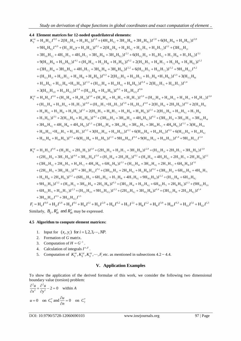
4.4 Element matrices for 12-noded quadrilateral elements: 0,0 1,0 2,0 3,0

2 2 2 5 2 5 5 5 2 9 2 9 5 9 5 9

4,0 0,1 1,1

9 9 2 4 2 4 4 5 4 5 2 7 2 7 11 2

11 2 5 7 5

H H 2(H H H H ) (4H H 3H H 3H H ) 6(H H H H )

9H H (H H H H ) 2(H H H H H H H H ) (3H H

3H H 4H H 4H

xx

ij i j j i i j i j j i i j j i i j

i j j i i j j i i j j i i j j i

i j j i i

K I I I I

I y I I

2,1 3,1

7 4 9 4 9 11 5 11 5 7 9 7 9

4,1 0,2 1,2

11 9 11 9 4 4 2 8 2 8 4 7 4 7 5 8 5 8

11 4 11 4 7 7 8 9 8 9

H 3H H 3H H ) 6(H H H H H H H H )

9(H H H H ) (H H H H H H ) 2( H H H H H H H H )

(3H H 3H H 4H H 3H H

3 H H

j j i i j j i i j j i i j

j i i j i j j i i j j i i j j i i j

j i i j i j j i i

I I

I I I

2,2 3,2 4,2

11 7 11 7 11 11

0,3 1,3

12 2 12 2 4 8 4 8 12 5 12 5 7 8 7 8 11 8

2,3 0,4

11 8 12 9 12 9 12 4 12 4 8 8

) 6(H H H H ) 9H H

(H H H H H H H H ) 2(H H H H H H +H H ) 3(H H

H H H H +H H ) (H H H H H H )

2(

H

j j i i j i j

j i i j j i i j j i i j j i i j j i

i j j i i j j i i j i j

I I I

I I

I I

1,4

12 7 12 7

2,4 0,5 0,6

11 12 11 12 12 8 12 8 12 12

H H H )

3(H H H H ) (H H H H ) H H

j i i j

j i i j j i i j i j

I

I I I

0,0 1,0 2,0 3,0

3 3 3 4 3 4 4 4 3 7 3 7 11 3 11 3 4 7 4 7

4,0 5,0 6,0 0,1

11 4 11 4 7 7 11 7 11 7 11 11 3 6 3 6 4 6

H H (H H H H ) (H H H H H H ) (H H H H H H H H )

(H H H H H H ) (H H +H H ) H H 2(H H 2H H ) 2(H H

yy

ij i j j i i j i j j i i j j i i j j i i j

j i i j i j j i i j i j j i i j j i

K I I I I

I I I I

1,1 2,1

4 6 3 8 3 8 6 7 6 7 4 8 4 8 11 6 11 6 7 8

3,1 4,1 0,2

7 8 11 8 11 8 10 3 10 3 6 6 12 3 12 3 10 4

H H H H H H ) 2(H H H H H H H H ) 2(H H H H H H

H H ) 2(H H H H ) (3H H 3H H 4H H ) (3H H 3H H 3H H

i j j i i j j i i j j i i j j i i j j i

i j j i i j j i i j i j j i i j j i

I I

I I I

1,2 2,2

10 4 6 8 6 8 12 4 12 4 10 7 10 7 8 8 10 11

3,2 4,2 0,3

10 11 12 7 12 7 11 12 11 12 10 6 10 6 12 6 12 6

3H H 4H H 4H H ) (3H H 3H H 3H H 3H H 4H H ) 3(H H

H H +H H H H ) 3(H H H H ) 6(H H H H ) 6(H H H H

H

i j j i i j j i i j j i i j i j j i

i j j i i j j i i j j i i j j i i j

I I

I I I

1,3 2,3 0,4 1,4 2,4

10 8 10 8 12 8 12 8 10 10 10 12 10 12 12 12H H H ) 6(H H H H ) 9H H 9(H H H H ) 9H Hj i i j j i i j i j j i i j i jI I I I I

0,0 1,0 2,0 3,0

2 3 2 4 3 5 4 5 2 7 3 9 11 2 5 7 4 9

4,0 5,0 0,1 1,1

11 5 7 9 11 9 3 4 2 6 4 4 5 6 3 7 2 8

H H (H H 2H H ) (2H H H H 3H H ) (H H 2H H 3H H )

(2H H 3H H ) 3H H (H H 2H H ) (H H 4H H 2H H 2H H )

xy

ij i j i j j i j i i j j i j i i j j i

j i j i j i j i i j i j i j j i i j

K I I I I

I I I I

2,1 3,1

11 3 4 7 4 7 5 8 6 9 11 4 11 4 7 7 8 9

4,1 5,1 0,2

11 7 11 7 11 11 10 2 4 6 3 8 12 2 10 5 6 7

4 8

(3H H 2H H H H 4H H 6H H ) (H H 3H H 2H H 6H H )

(2H H 3H H ) 3H H (3H H 2H H H H ) (3H H 6H H 4 H H

H H

i j j i i j i j j i j i i j i j j i

j i i j i j j i i j j i j i j i j i

j

I I

I I I

1,2 2,2

4 8 12 5 11 6 7 8 7 8 10 9 11 8 11 8

3,2 0,3 1,3

12 9 12 3 10 4 6 8 12 4 12 4 10 7 8 8 10 11

12 7 1

2H H ) (6H H 6H H H H 4H H 9H H ) (H H 6H H

9H H ) (H H 3H H 2H H ) (3H H H H 6H H 2H H ) (9H H

6H H H

i i j j i i j j i i j j i j i i j

j i i j j i j i j i i j j i i j j i

j i

I I

I I I

2,3 3,3 0,4 1,4

2 7 11 12 11 12 12 6 10 8 12 8 12 8

0,5 1,5

10 12 12 12

H ) (H H 9H H ) (2H H 3H H ) (3H H 2H H

)

3H H 3H H

i j j i i j i j j i j i i j

j i i j

I I I I

I I

0,0 1,0 0,1 1,1 2,0 0,2 2,1 1,2 3,0 0,3 3,1 1,3

1 2 3 4 5 6 7 8 9 10 11 12H H H H H H H H H H H Hi i i i i i i i i i i i iF I I I I I I I I I I I I

Similarly, , and x y

ij ijk ijkB R R may be expressed.

4.5 Algorithm to compute element matrices:

1. Input for ( , ) for 1,2,3, , .i ix y i NP

2. Formation of G matrix.

3. Computation of1H G .

4. Calculation of integrals,I .

5. Computation of , , , ,xx yy xy

ij ij ij iK K K F etc. as mentioned in subsections 4.2 4.4.

V. Application Examples To show the application of the derived formulae of this work, we consider the following two dimensional

boundary value (torsion) problem: 2 2

2 22 0 within

u uA

x y

*

10 on u C and *

20 on u

Cn



where *

1C and *

2C constitute the cross-section boundaries.

5.1 Finite Element Equation:

The field variable u (say) governing the physical problem is

1

( , )NP

i i

i

u u N x y

where ( , )iN x y are shape functions (as given) and

4 for the 4-noded quadrilateral



NP

By using the Galerkin weighted residual FE procedure, we achieve the following finite element equations,

[ ]{ } { }K u F

where the components of matrix [ ]K and{ }F are

ij ij

ij xx yyK K K and 2 ( , )i iA

F N x y dxdy

5.2 Finite Element Procedure:

The calculation process consists of the following steps

(i) For each element obtain componentsijK and

iF

(ii) Obtain the global FE equations for the whole system by assembling element equations.

(iii) Impose boundary conditions and solve for the generalized stress vectors of the whole system.

(iv) Calculate the torsional constant k for which 2A

k udxdy

5.3 Test Problems:

Three examples of solid cross-sections studied in [11] for which either exact or approximate and also FE

solutions exists are presented. A measure of error,kE is provided when an exact solution of the torsional

constant k is available. Where

exact

100 1k

kE

k

Example-1: A trapezoidal cross-section: The cross-section is modeled by 4-noded, 8-noded and 12-noded quadrilaterals as shown in Fig. 5.1. Computed

stress function values and the torsional constant k are tabulated in Table-1. Calculated value of k is in

agreement with the result of [11, 17 22].

(a) The FE model-1 with four 4-noded elements



(b) The FE model-2 with four

8-noded elements

(c) The FE model-1 with four

12-noded elements

Fig. 5.1: A trapezoidal cross-section and the FE models with four 4-noded, 8-noded

and 12-noded element and global nodes

Table-1

Computed stress function value(s), torsional constant k for example-1.

FE Model No Ui values Computed Torsion

Constant k

1 U5 0.20411036036036 0.112106069137319

2

U7 0.131915219488211 U12 0.130011182721599

0.163774369530811 U10 0.128537807516107 U15 0.128809621180074

U11 0.145877253027271

3

U9 0.10503448562457 U18 0.148355120939095

0.168497771701865

U12 0.149353737686098 U19 0.103180046293444

U15 0.101015314201091 U22 0.15129104422434

U16 0.147387025495711 U25 0.102964955448969

U17 0.150753644844546

Above table shows very good convergence in the calculation of Prandtle stress function values and the torsional

constant. We wish to declare that the solution for torsional constant k may be accepted as the best approximate

solution.

Example-2: A square cross- section:

The physical geometry and FE models are shown in Fig.5.2 This cross-section has four axes of symmetry;

therefore, only one-eighth of the cross-section needs to be analyzed. This fractional portion is divided into three

elements (Fig.5.2(a-c)).We wish to note that at least to the knowledge of present authors the octant of a square

had been modeled first time by three quadrilateral elements in [17,20]. Computed results are tabulated in Table-

2.

(a) Axes of symmetry of a

square cross-section

(b) The FE model-1 with three

4-noded quadrilateral elements



(c) The FE model-1 with three

8-noded quadrilateral elements

Fig. 5.2: The octant of a square cross-section and element subdivision

Table-2

Computed stress function values, torsional constant k and error kE for example-2

FE Model

No

Ui values Computed Torsion

Constant k

kE

1

U1 0.15768290 U4 0.0900712

0.1303802725

7.28512% U2 0.11872934 U5 0.074753

2

U1 0.1471286244 U9 0.0904859

0.14043709218

0.133623% U2 0.139599417 U10 0.0878646

U3 0.114156447 U11 0.07971913

U4 0.0698718347 U12 0.04339872

U6 0.1317489 U14 0.036225977

U7 0.09980412 --- --------------

Exact torsion constant k = 0.140625

It is to be noted that the results are in good agreement compare to [17, 20] because element matrices are exactly

obtained.

Example-3: An equilateral triangular cross-section:

Fig. 5.3: The one third of an equilateral triangular cross-section and element subdivision



The cross- section and FE models are shown in Fig.5.3. Due to symmetry, only one third of the original model is

used. u = 0 is specified on sides AC and CD and 0u

n

enforced at the lines of symmetry: sides AB and BD.

Calculated stress function values ui and the torsional constant k are given in Table-3.

Table-3

Computed stress function values, torsional constant k and error kE for example-3

FE

Model

No

Ui values

Computed Torsion

Constant k

kE

1 U5 0.0234375 ---- 0.140625 549.519%

2

U4 0.0008896 U6 0.0240287

0.0193514660942148

10.6194% U5 0.03883635 ----

3

U5 0.03555065 U8 0.02154

0.0220314297875825

1.7588% U6 0.03914403 U9 0.0039038

U7 0.02178696 ----

Exact torsional constant is k = 0.021650635

Example-4: An elliptic cross-section:

The cross-section and FE models are shown previously in Fig. 3.8 and Fig. 3.8.2. Due to symmetry, only one-

fourth of the cross-section is considered for FE models. Computed results are given in Table-4.

Table -4

Computed Prandtl stress values Ui and torsional constant k and error kE , for example-4

FE Model No Ui values Computed Torsion

Constant k

kE

1

U1 4.9755174 U4 4.761976

142.827008323399

5.239% U2 2.8884254 U5 1.177573

2

U1 3.265994 U9 1.906576

136.882566278808

0.8589%

U2 3.29038 U10 2.527975

U3 2.871832 U11 1.90699

U4 1.6818382 U12 1.10534

U6 2.870329 U13 1.0914

U7 2.5464496

Exact torsion constant k = 135.716802635079

We wish to remark here all the computed results tabulated in Tables (1)-(4) are more accurate comparing with

the results reported in [11, 16, 18-22].

VI. Conclusion The strong mathematical foundation of Finite Element Method based on shape functions. The

derivations of polynomial shape functions in local co-ordinates are comparatively easier than that of in global

co-ordinates. Common practice is the use of polynomial shape functions in local co-ordinates in transformation

equations. In such instances complications arise from two main sources, firstly the large number of integrations

that need to be performed and secondly, in methods which use isoparametric/ subparametric/ superparametric

elements, the presence of the determinant of the Jacobean matrix in the denominator of the stiffness matrix for

which the integrands are rational functions. Precisely, to form the element stiffness matrices we are required to

evaluate numerous rational integrals. Analytical integration schemes are available only for the integral of

bivariate polynomial numerators with bilinear denominators. In practical situation that employs higher order



elements, all the integrals are rational with the denominator of higher order bivariate expressions. Such rational

integrals cannot be evaluated analytically and we are bound to employ the Gaussian quadrature schemes.

Obviously, for the desired accuracy of evaluations the number of Gaussian points and weights are needed to be

increased and that increases substantially the computing time. Hence, a proper balance between the accuracy

and efficiency is an important task. Further, an attention is always required to select the order of the integrating

rule as it is not yet totally worked out.

A suitable alternative, the use of polynomial shape functions in global coordinates in the formulation

give rise integrals of polynomials which can be exactly evaluated either by the selected order of the gauss

quadrature rule or by analytical schemes. In this case the main barrier is the derivation of shape functions in

global coordinates for the element under considerations. Especially it is very much difficult and so cumbersome

in case of the quadrilateral elements. Considering all the facts and the popularity of the quadrilateral elements,

we have concentrated to derive polynomial shape functions in global coordinates and to present all the

components of element matrices in bivariate polynomial form in a systematic way. So that one can use the

gaussian quadrature schemes or other numerical schemes easily for exact computing all the element matrices.

The technique so developed in this study is as: (1) formation of a matrix G (say) by the global nodal co-

ordinates of the element geometry and then its inverse matrix H (say), and (2) the values of the integral of

monomials over the element. Finally, we have employed analytical schemes and presented all the components of

element matrices as the expressions of products of components of matrix H. Thus, it can be stated shortly that

once the matrices G, H are formed and values of the integrals of monomials over the element are evaluated then

the computation of element matrices are simply done by the product of components of matrix H only. So, it

reduces many time consuming steps of FEM solution procedure and finally that reduces substantially the

computational effort.

It has been clearly shown for the first time that the matrix G is singular for two types of element

geometry for which bilinear shape functions (for 4-noded quadrilateral) cannot be derived but that of higher

order (for 8-noded, 12-noded quadrilaterals) shape functions can be derived. Furthermore, geometrical reasons

are also shown for which the matrix G is bad scaled. Through demonstrations of different type of element

geometry, it has been found that such difficulties in case of derivation of shape functions may be surmounted

only by changing the mesh of the domain. Hence, sincere care is needed in case of deriving polynomial shape

functions in global co-ordinates for quadrilateral elements that is to ensure the matrix G is nonsingular. One can

easily apply the technique to derive polynomial shape functions in local co-ordinates by forming G matrix by

the local nodal co-ordinates.

The present technique so presented to compute element matrices exactly is easy for computer coding, a

computer code in MATLab® is developed which is not included here with. The accuracy and efficiency of the

formulae so presented are then demonstrated through the calculation of Prandtl stress function values and

torsional constant of different type of cross sections. Comparison of computed results with the results of other

researchers clearly exhibits the best accuracy of the present technique. Since explicit expressions for all types of

element matrices are presented, we believe that the technique of this basic study will be contributing and

attractive in the realm of application of the finite element method.

References [1]. Zienkiewicz, O.C.and Cheungy.K.,The Finite Element in the Solution of Field Problems.(The Engineer, 220: pp. 507-510, 1965).

[2]. Okabe ,M., Complete Lagrange Family for the Cube in Finite Element Interpolations, Comput. Methods Appl. Mech. Engg. 29, 1981, 51-56.

[3]. Okabe, M., Analytical Integration Formulae related to Convex Quadrilateral Finite Elements, Comput. Methods Appl. Mech. Engg.

29, 1981, 201-218. [4]. Zienkiewicz, O.C.and Morgan, K., Finite Element and Approximation. (John Wiley & Sons, Inc., New York, 1983).

[5]. Babu, D. and Pinder, G.F., Analytical integration formulae for linear isoparametric finite elements, Int. J. Num. Meth. Engg., 20,

1984, 1153-1166. [6]. Reddy,J.N., An Introduction to the Finite Element Method. (New York: McGraw –Hill Book Company, 1984).

[7]. Rathod ,H.T., Some Analytical Integration Formulae for a Four-node Isoparametric Element, Computers and Structures, 30, 1988, 1101-1109.

[8]. Hacker,W.L. and Schreyer, H.L., Eigen Value Analysis of Compatible and Incompatible finite Elements, Int. J. Num. Methods

Engg., 28, 1989, 687-703. [9]. Zienkiewicz, O.C.and Taylor ,R.L.,The Finite Element Method .(4th ed., Maidenhead, UK: McGraw –Hill Book Company 1989).

[10]. Yagawa ,G.Ye.,G.W.and Yashimara,S., A Numerical Integration Scheme for Finite Element Method Based on Symbolic

Manipulation, Int. J. Num. Methods Engg., 29, 1990, 153-159. [11]. Nguyen, S.H., An accurate finite element formulation for linear elastic torsion calculations, Computer and Structures, 42(5), 1992,

707-711.

[12]. Griffths, D.V., Stiffness Matrix of the Four-node Quadrilateral Element in Closed Form, Int. J. Num. Methods Engg., 37, 1994, 1027-1038.

[13]. Griffths, D.V. and Mustoe ,G.G.W., Selective Reduced Integration of Four-node Plane Element in Closed Form, J. Engg. Mech.,

121(6), 1995, 725-729. [14]. Videla, N. Aparicio and M. Carsolaza, (1996) Explicit Integration of the Stiffness Matrix of Four-noded-plane-elasticity Finite

Element, Int. J. for Numer. Methods in Bio. Engg., 12(11), 1996, pp. 721-743.



[15]. Lague, G. and Baldur, R., Extended Numerical integration method for triangular surface, Int. J. Num. Methods Engg., 11, 1997,

388-392.

[16]. Rathod ,H.T.and Islam, M.S., Integration of Rational Functions of Bibrate Polynomial Numerators with Linear Denominators over a (-1,1) Square in a Local Parametric Space, Computer Methods in Appl. Mech. Engg., 161(1-2), 1998, 195-213.

[17]. Barrett, K.E., Explicit Eight_nodded Quadrilateral Elements, Finite Elements in Analysis and Design, 31, 1999, 209-222.

[18]. Karim ,M.S., Integration of Some Bivariate Polynomials with Rational Denominators- An Application to Finite Element Method, Doctoral diss., Dept. of Meth., Bangalore University , Banglalore-560001 ,India, 2000.

[19]. Rathod,H.T and Karim, M.S., Synthetic Division based Integration of Rational Functions of Bivariate Polynomial Numerators with

Denominators over a unit triangle {0 , 1, 1} In the Local Parametric Space ( , ) , Computer Methods in Appl. Mech.

Engg. 181(1-3), 2000, 191-235.

[20]. Rathod, H.T. and Sridevi Kilari, General Completed Lagrange Family for the cube in Infinite Element Interpolations, Computer

Methods in Appl. Mech. Engg., 181(1-3), 2000, 295-344. [21]. Rathod , H. T. and Karim ,M.S., An Explicit Integration Scheme based on Recursion for the Curved and Matrix Multiplication for

the Linear Convex Quadrilateral Elements, Int. J. on Computational Engg. Sci. (JCES), 2(1), 2001, 95-135.

[22]. Rathod, H. T. and Karim, M.S., An Explicit Integration Scheme based on Recursion for the Curved Triangular Finite Elements, Computers and Structures , 80(1), 2002, 43-76.

[23]. G. Dasgupta, Stiffness Matrices of Isoparametric Four-node Finite Elements by Exact Analytical Integration. ASCE, 21(2), 2008,

54-50.

study on derivation of shape functions in global … be performed and secondly, in methods which use...

Documents