study on flood para-tank model parameters with …jihmsp/2015/vol6/jih-msp-2015-05-008.pdf · study...

Journal of Information Hiding and Multimedia Signal Processing c©2015 ISSN 2073-4212

Ubiquitous International Volume 6, Number 5, September 2015

Study on Flood Para-Tank Model Parameters withParticle Swarm Optimization

Po-Yuan Hsu

Department of Civil EngineeringNational Pingtung University of Science and Technology, NPUSTand National Kaohsiung University of Applied Sciences, KUAS

415 Chien-Kung Road, Kaohsiung, 807, [email protected]; [email protected]

Yi-Lung Yeh

Department of Civil EngineeringNational Pingtung University of Science and Technology, NPUST

1 Shuefu Road, Neipu, Pingtung 91201, [email protected]

Received March, 2015; revised May, 2015

Abstract. The relationship between rainfall and runoff has been the most importantpart of hydrological analysis. It is easier to get rainfall than to get runoff; therefore,the methods of calibration analysis regarding their relationship were actively developedin previous research to simulate the runoff with rainfall data. In this study, the conceptof tank model mechanism serves as a starting point to convert the original basic type offour tank sections into a combination of aboveground and underground mechanisms toaddress a higher proportion of impermeable layer in cities. A concept similar to a tankis used to establish the operational mechanisms produced after rainfall on the surface. Itis simulated in the underground sewer system after overland flow, and therefore, a newrainfall-runoff model is established, called the Para-Tank Model (PTM). The particleswarm optimization (PSO) from the modern stochastic optimization algorithms derivedfrom natural biological group behaviors is employed to calculate the parameter valuesrequired by PTM. In this example, this method plots the calculated and target flows ex-cellently according to the time axis. Its fast convergence, high calibration precision, andstable calculation results help to significantly improve the efficiency of automatic param-eter calibration. Therefore, it is presented as a viable method for optimization, whichcan be extended to other hydrological models.

Keywords: Tank model, Rainfall-runoff, Particle Swarm Optimization, PSO

1. Introduction. In general, hydrological models simulating hydrological phenomenacan be divided into black-box model, physically based model, and conceptual model ac-cording to the level of fidelity. The conceptual model is between the first two, and the tankmodel belongs to this model. Therefore, the original concept of the tank model is used inthis study to reasonably represent the characteristics of the hydrologic system within aregion with its simplified logic architecture. The runoff mechanism for both abovegroundand underground scenarios is used to simulate the rainfall-runoff relationship within theregion so as to develop a new hydrological model called Para-Tank Model (PTM).In the past, the calibration of tank model parameters mainly depended on trial and error.

911

912 P. Y. Hsu, and Y. L. Yeh

It is time consuming and laborious when a parameter is adjusted based on the accu-mulation of experiences. However, with the advancement of computer technology andmathematical optimization techniques, the parameter calibration technique based on au-tomatic optimization has been introduced to the hydrological model. The optimizationmethod developed on the basis of scientific observation of biological group behavior hasbecome a new research direction. The particle swarm optimization (PSO) developed onthe basis of the predatory behavior of birds by Kennedy and Eberhart [1] in 1995 is asimplified simulation model of society, which moves the individuals of the population toa better area on the basis of the level of their adaptation to the environment. In [2], Shiand Eberhart further improved the performance of PSO. Many extensions have also beenproposed and can be classified as three types, 1) Discrete PSO [3], 2) Niche PSO [4] and 3)Hybrid PSO. Discrete PSO is the method that focuses on the problem of combination op-timization. Niche PSO can handle premature convergence problem and slow convergence.Hybrid PSO integrates artificial intelligence technique like Genetic Algorithm, SimulateAnneal Arithmetic, Neural networks, and so forth with PSO, which includes SelPSO,BreedPSO and Simulate Anneal-PSO (SA-PSO). Bekele et al. [5] in 2005, Gill et al. [6]and Jiang Yan et al. [7] in 2006, and Chen Qiang [8] in 2010 applied PSO in parametercalibration of hydrology models and obtained good results; this proved its versatility inparameter calibration of different hydrological models. Therefore, in this paper, PSOwill be used for quick, reasonable, and stable calibration of PTM parameters. The fourparameters H1 , λ1 , H2 , and, λ2 , are used to calculate the ratio of calculated flow totarget flow, indicating that the operating mechanism of PTM can meet the rainfall-runoffrelationship. It is a good start for the development of future models.In the following sections, we introduce the model theory in Section 2. Section 3 brieflyreviews PSO and presents the method for discovering the values of model parameters.Section 4 provides an evaluation and discussion of the method. Section 5 presents theconclusions.

2. Model Theory. In a brief rainstorm, it is difficult for a city to determine the physicalmeaning of 16 tank model parameters. Japanese literature recorded cases of urban floodoutflow analysis with a two-stage tank, and the Chinese scholar R. S. Chen [9] studiedthe cases and proposed amendments to the urban tank model. Inspired by this concept,we changed the model into a dual mechanism for both aboveground and undergroundscenarios. A concept similar to tank is used to establish the operational mechanismsproduced after rainfall on the surface. It is simulated in the underground sewer systemafter overland flow, and therefore, a new rainfall-runoff model is established.

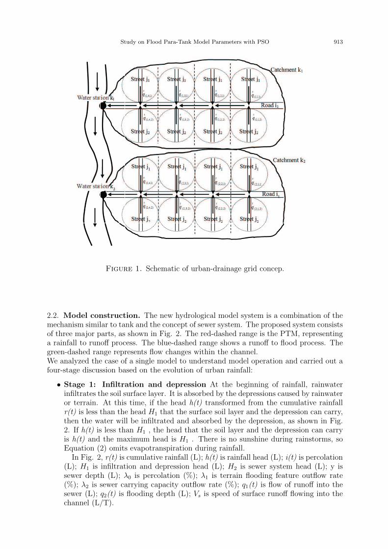
2.1. Concept of catchment grid model. The regional drainage concept dominatesurban drainage system. Since urban tank is feasible, it could take the drains under mainroads (i) as its mains to collect the water from street (j). Under this concept, it couldconsider an inter-mesh grid formed between sewers as a model unit. The sewer flow ineach grid unit qt(k,i,j) ,enters the main drains after collection. Then calculations of thesewer water system are performed. If it expands to k catchment areas, calculations of theopen-channel system are performed. In Fig. 1, the entire region contains k catchments, inwhich main roads (i) and street (j) form many grids according to the flow and configurationof regional drainage. Each grids sewer flow is qt(k,i,j) . When rainwater flows through the

ground into the sewers, the flows are qt(1,1,1) , qt(1,1,2) , qt(1,2,1) .... , qt(k,i,j) and the total flow of

the drainage system in the kth catchment is∑l,m

1 qt(i,j) . Calculations of the sewer watersystem are then performed.

Study on Flood Para-Tank Model Parameters with PSO 913

Figure 1. Schematic of urban-drainage grid concep.

2.2. Model construction. The new hydrological model system is a combination of themechanism similar to tank and the concept of sewer system. The proposed system consistsof three major parts, as shown in Fig. 2. The red-dashed range is the PTM, representinga rainfall to runoff process. The blue-dashed range shows a runoff to flood process. Thegreen-dashed range represents flow changes within the channel.We analyzed the case of a single model to understand model operation and carried out afour-stage discussion based on the evolution of urban rainfall:

• Stage 1: Infiltration and depression At the beginning of rainfall, rainwaterinfiltrates the soil surface layer. It is absorbed by the depressions caused by rainwateror terrain. At this time, if the head h(t) transformed from the cumulative rainfallr(t) is less than the head H1 that the surface soil layer and the depression can carry,then the water will be infiltrated and absorbed by the depression, as shown in Fig.2. If h(t) is less than H1 , the head that the soil layer and the depression can carryis h(t) and the maximum head is H1 . There is no sunshine during rainstorms, soEquation (2) omits evapotranspiration during rainfall.

In Fig. 2, r(t) is cumulative rainfall (L); h(t) is rainfall head (L); i(t) is percolation(L); H1 is infiltration and depression head (L); H2 is sewer system head (L); y issewer depth (L); λ0 is percolation (%); λ1 is terrain flooding feature outflow rate(%); λ2 is sewer carrying capacity outflow rate (%); q1(t) is flow of runoff into thesewer (L); q2(t) is flooding depth (L); Vs is speed of surface runoff flowing into thechannel (L/T).


Figure 2. Dual model system of para-tank mechanism and sewer drainage system.

∆r(t) = r(t) − r(t− 1) (1)

h(t) = h(t− 1) + ∆r(t) (2)

When h(t) ≤ H1, q1(t) = 0 (3)

q2(t) = 0 (4)

• Stage 2: Percolation When the rainfall continues increasing to the maximumhead that the surface soil layer infiltration and depression can carry (H1) , it willpercolate downward to the aquifer below. In Fig. 2, i(t) is the downward amountof percolation, and λ0 is the percolation proportion. At the beginning, the down-ward amount of percolation i(t) is high (the slope of percolation proportion, λ0 ,is relatively high), but when the air is squeezed under the ground, it will reducethe post-percolation, which approaches a constant value (the slope of percolationproportion, λ0 , approaches 0). In Fig. 3, at the beginning, the downward percola-tion proportion, λ0 , is high, the amount of percolation, i(t), increases rapidly, butapproaches a constant value at a later stage, so in the case of a quick urban storm,it is reasonable to assume that the amount of percolation i(t) will quickly becomea constant value, which speeds up the whole model simulation by eliminating thevariable λ0 .

i(t) = C (5)

Where i(t) is the amount of percolation (mm) and C is a constant.

• Stage 3: Overland flow When rainfall continues increasing, it will generate anoverland flow as the rainstorm exceeds the percolation rate of the aquifer at Stage2. The water will flow into the citys drainage system and test its capacity. Wethen performed the calculations of the sewer system flow. In Fig. 2, when head h(t)is greater than H1 , subtract the maximum head H1 at Stage 1 and the amount ofpercolation i(t) at Stage 2 and multiply by the outflow rate λ1 to obtain the overlandflow q1(t). When the overland flow enters the citys sewer system, there is a manholeinflow velocity, namely Vs, which can be defined as the velocity of surface runoff.After the two are multiplied, q1(t) Vs will develop into a constant amount that flowsinto the sewer system, forming a pipe flow with a height of y, and H2 can be regardedas the maximum head of the sewer system.


Figure 3. Changes in the amount of percolation i(t) depending on rainfalltime t.

When H1+H2≥ h(t)> H1,

q1(t) = ((h(t) −H1 − i(t)) × λ1 (6)

q2(t) = 0 (7)

• Stage 4: Flooding After Stage 1, 2, and 3, rainfall continues increasing, and willexceed the design head of the city sewer system H2 by which time the flooding begins.In Fig. 2, when head h(t) is greater than H1+H2 , subtract the maximum head H1 atStage 1, the amount of percolation i(t) at Stage 2 and the sewer system head H2 atStage 3, then multiply by the outflow rate of the sewer carrying capacity λ2 , wewill get the flow depth of the flooding q2(t) . At this point, the maximum carryingcapacity of the sewer system q1(t) needs to be corrected to the design capacity qc ,which can be set at a constant value.

When h(t)>H1+H2,

q1(t) = ((h(t) −H1 − i(t)) × λ1 ≤ qc (8)

q2(t) = ((h(t) −H1 − i(t) −H2) × λ1 × λ2 (9)

Where qc is the sewer systems design capacity (L).At Stage 3 and 4, after multiplied by speed Vs , the overland flow q1(t) entersthe sewer system, and then, we started the channel calculation process. To getthe accurate velocity V and depth y, we can solve a one-dimensional Saint-Venantvariable flow equation as follows:

q1(t) × Vs +∂Q

∂x+∂A

∂t= 0 (10)

1

g

∂V

∂t+V

g

∂V

∂x+∂y

∂x= S0 − Sf (11)

Equations (10) and (11) are the continuous equation and momentum equation ofOne-dimensional Gradually Varied Unsteady Flow under the assumption of no lateralflow, where Q is the flow (L3/T ) , V is the average velocity of the section (L/T ) ,t is the time coordinate (T), n is Manning roughness coefficient (TL−1/3) , So isthe vertical gradient of the channel bottom , x is the space coordinate in the flowdirection (L), y is the depth (L), g is the gravitational acceleration (L/T 2) , R ishydraulic radius (L), Sf is the energy gradient line (L/L) , and can be calculatedusing Manning formula, namely,


Sf =V 2n2

R4/3(12)

We thus built the proposed model based on the aforementioned three sectionsand four stages. The parameters of the model all have a certain degree of physicalsignificance. The model is a combination of the mechanism similar to tank and theconcept of sewer system. Since the model is built upon the tank model, it is calledthe PTM.

3. Optimization Method.

3.1. Particle Swarm Optimization (PSO). In this study, the optimization of param-eter calibration uses PSO, developed on the basis of the discovery of an evolutionaryadvantage of the population regarding information sharing from the observation of thesocial behaviors of animals. The principle moves the individuals of the population to agood area based on the level of their adaptation to the environment. It does not apply anevolution operator to the individuals, instead it views each individual as a particle with-out volume in d-dimensional search space, flying at a certain speed that is determinedaccording to its own flying experience and that of the other particles. The ith particleis represented as Xi = (Xi1, Xi2, . . . , Xid) . The best position that it has experienced,namely the position with the best fitness, is denoted by Pi = (Pi1, Pi2, . . . , Pid) , alsoknown as Pbest . The index number of the best-experienced position of all the particlesin the group is denoted by g, namely Pg, also called Gbest . The velocity of Particle iis represented by Vi = (Vi1, Vi2, . . . , Vid) . The dth dimension of each generation variesaccording to the following equations:

V t+1id = ωV t

id + c1rt1(P

tid − xtid) + c2r

t2(P

tgd − xtid) (13)

X t+1id = X t

id + V t+1id t (14)

Where w is inertia weight, c1 and c2 are acceleration constants, r1 and r2 are two randomvalues changing in the range [0,1]. If the velocity of a particle that is accelerated in somedimension Vid exceeds the maximum velocity Vmax,d, then the dimensional velocity is setto the maximum velocity for that dimension Vmax,d.In Equation (13), the first part is the previous behavior inertia of particle; the secondpart is a cognition part, which means the self-reflection of particle; and the third partis a social part, which means the information sharing and mutual cooperation betweenparticles. The PSO algorithm is like a psychological assumption: in the cognitive processof seeking consistency, individuals tend to take into account the faith of their coworkerswhile maintaining their own beliefs. When perceiving that the faith of their coworkersis better, they will adjust adaptively. As shown in Fig.4, the particle has its originalvelocity V t

id and X tid, together with its past experience. It finally moves to the best

position after referring to the current local optimal solution Pbest (cognition part) aswell as the information sharing and mutual cooperation of the current global optimalsolution Gbest (social part).


Figure 4. Schematic diagram of PSO.

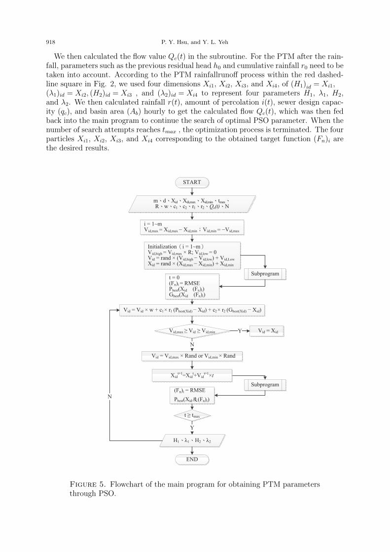
3.2. Parameter optimization of the proposed model system. Every grid in thecity represents a catchment. To start with, we analyzed and studied just one single gridmodel in order to verify its feasibility. The improvements have been made to PSO inthe last 20 years, but the basic principle remains the same, so this study still selects theparameters based on a combination of the basic PSO and PTM operation while usingMatlab programming language as a development tool. The design process consists of amain program as shown in Fig. 5 and a subroutine as shown in Fig. 6.The basic input data include the number of particles (m), dimension count (d), unknownvariables (Xid), i=1-m, position range (Xid,max, Xid,min), the number of times (tmax), speedcorrection (R), inertia weight (w), global acceleration constants (c1, c2), and randomlygenerated numbers (r1), (r2). Historical hydrographic data require target flow Qo(t)and target number (N, with 1 hour as the unit) to establish the speed range of eachparticle. Generally, we assume that Xid,max = Xid,max −Xid,min, Vid,min = −Vid,min.Since there was no set value to begin with, we first started initialization by assumingthat Vid,high = Vid,max ×R, Vid,low = 0, Vid = rand× (Vid,high − Vid,low)Vid,low ,Xid = rand× (Xid,min −Xid,min)Xid,min. With the initial values, we then established thetarget function and used the historical hydrological data to optimize the parameters. It isbest when the difference between the calculated flow and the target flow is at its minimum.Considering the possibility that positive and negative values can cancel out each other,the target function uses the Root Mean Squared Error (RMSE)

RMSE =

√∑Ni=1(QC(t) −QO(t))2

N(15)

Where: Qc(t) stands for the calculated flow; Qc(t) stands for the targeted flow and; Nstands for the number of data points.

After initialization, we can get the local optimum Pbest [ Xid and (Fn)i ] and the groupoptimum Gbest [ Xid and (Fn)i ] of the target function between the particles, and thenadjust the speed and position through Equations (13) and (14) according to the PSOprinciple to get better local optimum Pbest and group optimum Gbest.


We then calculated the flow value Qc(t) in the subroutine. For the PTM after the rain-fall, parameters such as the previous residual head h0 and cumulative rainfall r0 need to betaken into account. According to the PTM rainfallrunoff process within the red dashed-line square in Fig. 2, we used four dimensions Xi1, Xi2, Xi3, and Xi4, of (H1)id = Xi1,(λ1)id = Xi2, (H2)id = Xi3 , and (λ2)id = Xi4 to represent four parameters H1, λ1, H2,and λ2. We then calculated rainfall r(t), amount of percolation i(t), sewer design capac-ity (qc), and basin area (Ab) hourly to get the calculated flow Qc(t), which was then fedback into the main program to continue the search of optimal PSO parameter. When thenumber of search attempts reaches tmax , the optimization process is terminated. The fourparticles Xi1, Xi2, Xi3, and Xi4 corresponding to the obtained target function (Fn)i arethe desired results.

START

m d Xid Xdi,max Xid,min tmax

R w c1 c2 r1 r2 Qo(t) N

i = 1~mVid,max = Xid,max Xid,min Vid,min = Vid,max

Initialization i = 1~mVid,high = Vid,max × R; Vid,low = 0Vid = rand × (Vid,high Vid,low) + Vid,Low

Xid = rand × (Xid,max Xid,min) + Xid,min

Vid = Vid × w + c1 × r1 (Pbest(Xid) Xid) + c2 × r2 (Gbest(Xid) Xid)

Subprogramt = 0(Fn)i = RMSEPbest(Xid (Fn)i)Gbest(Xid (Fn)i)

Vid,max ! Vid ! Vid,min Vid = Xid

Vid = Vid,max × Rand or Vid,min × Rand

Subprogram

Xidt+1

=Xidt+Vid

t+1×t

(Fn)i = RMSE

Pbest(Xid (Fn)i)

t tmax

H1 "1 H2 "2

END

Y

N

Y

N

Figure 5. Flowchart of the main program for obtaining PTM parametersthrough PSO.


Subprogram START

h0 r0 r(t) i(t) qc Ab

Xid i = 1~m d = 4(H1) id = Xi1 1)id = Xi2

(H2) id = Xi3 2)id = Xi4

r(t) = r(t) r(t 1)

h(t) = h(t 1) + r(t)

h(t) H1q1(t)=0

q2(t)=0Y

H1 + H2 ! h(t) > H1q1(t)=(h(t) H1 i(t))× 1

q2(t)=0Y

q1(t)=(h(t) H1 i(t))× 1

q2(t)=(h(t) H1 i(t) H2)× 2

N

q1(t) qc

N

N

q1(t)=(h(t) H1 i(t))× 1q1(t) = qc

N

q = q1(t) + q2(t)

Qc(t) = q × Ab × (103/(N, hr*60*60))

h’(t) = h(t) ! i(t) !

h(t!1)=h’(t)

t = N

Qc(t)

Y

Subprogram

END

YN

Figure 6. Flowchart of the subroutine for obtaining PTM parametersthrough PSO.

4. Results of Parameter Calibration and Discussion.

4.1. Overview of the Regions Under Study. The study is carried out in the met-ropolitan area of Kaohsiung. The report of the Flood Control and Drainage Plan ofKaohsiung noted [10] that at 5:00 pm on July 11, 2001, the strong southwest flow intro-duced by Tropical Storm Trami set off 10 consecutive hours of heavy rain in Kaohsiungarea. According to the records of Cianjhen and Zuoying weather stations of the citys


Weather Bureau, the cumulative rainfall totals of these two areas are respectively 525mm (the highest single-day rainfall since 1962) and 493 mm. The 1-hour maximum rain-fall recorded at Zuoying Station is 126.5 mm, approaching the 130 mm standard for a100-year storm, and the 3-hour maximum rainfall is 329 mm, higher than the 300 mmstandard for a 200-year storm. The 1-hour maximum rainfall recorded at Cianjhen Sta-tion is 119.5 cm, and the 3-hour maximum rainfall is 239 mm. The rainfall records ofboth stations are much higher than the flood control and drainage design standards ofKaohsiung (5-year drainage and 20-year flood control). The drainage experienced furtherblocking caused by the tidal surge at the Love River estuarine, as a result, although theimplementation rate of urban stormwater sewer system reached over 90 percent, the sys-tem still failed to put the flood under control, resulting in severe flooding of 300 hectaresof low-lying areas of Yancheng District, Benguanli, Benheli, Baozhugou, No.2 Canal andCianjhen District. For a comparative analysis of PTM operation, PTM rainfall data andthe average of Kaohsiung, Zuoying and Fongshan rainfall stations during the 711 Floodfrom the Flood Control and Drainage Plan of Kaohsiung are taken as the rainfall r(t)values in the model for calculation, with the rainfall data shown in Table 1.

Table 1. Observed rainfall data during the 711 Flood.

Time Rainfall (mm) Time Rainfall (mm)Day Hour K.siung Zuoying Fongshan Average Day Hour K.siung Zuoying Fongshan Average

11

5 1.5 0.0 0.0 0.50

12

1 29.0 42.5 45.5 39.006 2.5 0.0 0.0 0.83 2 25.0 48.5 41.0 38.177 5.0 1.5 0.0 2.17 3 18.5 20.0 17.5 18.678 3.5 1.5 1.0 2.00 4 7.5 11.0 16.0 11.509 0.5 0.0 8.5 3.00 5 1.5 6.0 1.0 2.8310 0.0 1.5 3.5 1.67 6 1.0 1.5 6.0 2.8311 0.5 0.0 0.5 0.33 7 0.0 0.5 0.0 0.1712 0.0 0.5 0.0 0.17 8 0.0 9.5 0.0 3.1713 0.0 0.0 0.0 0.00 9 0.0 2.0 1.0 1.0014 0.0 0.0 0.0 0.00 10 2.0 0.0 0.5 0.8315 0.0 0.0 0.0 0.00 11 0.0 0.0 2.5 0.8316 2.0 0.5 4.5 2.33 12 0.0 0.0 0.0 0.0017 8.5 1.0 8.0 5.83 13 0.0 0.0 0.0 0.0018 26.0 3.0 39.0 22.67 14 0.0 2.0 0.0 0.6719 72.5 95.0 44.5 70.67 15 2.5 5.5 3.0 3.6720 43.0 107.0 29.5 59.83 16 0.0 0.0 2.0 0.6721 54.0 126.5 92.0 90.83 17 0.0 0.0 0.0 0.0022 65.5 22.0 81.0 56.17 18 0.0 0.0 0.0 0.0023 119.5 32.5 89.0 80.33 19 1.5 0.0 0.0 0.5024 66.0 44.0 64.0 58.00 20 0.0 0.0 0.0 0.00

In this study, the hydrological model PTM focuses on the impact of rainstorm onmetropolitan areas with a higher proportion of impermeable layer. The 711 Storm eventcan be used as a perfect case to discuss the parameter optimization of the model for urbanrainfallrunoff pattern. Kaohsiung area is mainly in the Love River basin. According to thedistribution of the flooded area in the 711 Flood, the basin is divided into nine catchmentsdepending on the terrain, as shown in Fig. 7. Catchment 3 is selected for the optimizationof PTM parameter calibration, as it has no differentiated subareas such as a and b. Wecalculated the rainfallrunoff in the catchment (HEC-1) using the measured rainfall records


as the sidestream boundary of channel flood routing model (NETSTARS) and the tidelevel hydrograph of Kaohsiung Port as the downstream water boundary to generate thewater level and discharge hydrograph of each Love River section. The flow value thusacquired is regarded as true in the PTM model and taken as the target of parametercalibration. The calculation model has a backwater effect, resulting in a small portion ofnegative flow values, so the backwater effect will not be considered for the current stageof the study.

Figure 7. Catchments in Love River basin.

4.2. Results of parameter calibration. We then fed the rainfall and flow of a catch-ment into the PTM analysis program. We assumed that the global acceleration con-stants c1 and c2 are both 0.1, the inertia weight w = 0.8, the particle count m = 30,the dimension count d = 4, the previous residual head h0 = 3 mm, the cumulative rain-fall r0 = 1 mm, and the amount of percolation i(t) is 1 mm. The sewer design capac-ity qc refers to the standard of the urban stormwater sewer system in Taiwan. Thestormwater sewer system of Kaohsiung was designed in 1976 by the former Bureau ofPublic Works of Taiwan Provincial Government, primarily based on the rainfall regres-sion analysis for 19481974, and the 1-hour 5-year storm intensity, 70.9mm/hr, is thedrainage-section design standard. Position range Xi1 represents the head of infiltrationand depression H1 and is set between 1 and 100, Xi2 represents the outflow rate of theterrain flooding feature λ1 and is set between 0 and 1, Xi3 represents the head of thesewer system H2 and is set between 50 and 100, Xi4 represents the outflow rate of thesewer carrying capacity λ2 and is set between 0 and 1, and number tmax is set to 1000 forthe actual calculation. The calculation results are H1= 3.745365, λ1 = 0.591964, H2 =52.16278, and λ2 = 0.240281; the target function (Fn)i reaches 3.66. The four parameterswere then fed back into PTM for hourly calculation to get the comparative results of thecalculated flow Qc(t) and the target flow Qo(t) , as shown in Fig. 8, which shows that itis feasible to obtain the PTM parameters by means of PSO.


Figure 8. Comparison of the calculated flow and the target flow.

4.3. Discussion. PSO is applied in this study to select the PTM parameters. In theFlood Control and Drainage Plan of Kaohsiung, the impact of the 711 Trami on Baozhugouof Kaohsiung can be shown by the fact that the parameters in this area are H1 =3.745365, 1 = 0.591964, H2 = 52.16278, and 2 = 0.240281. After assessment of themodel indicators, considering the time axis factor, we select the root mean squared error(RMSE), coefficient of efficiency (CE), and percent error of total volume (VER) of totaldata-point count for evaluation. The evaluative results depend on the error evaluation;when the closest RMSE value approaches 0, the better the model performs, and the moreCE approaches 1 or VER approaches 0, the better applicability the model has for therainfallrunoff process.

In this example, RMSE reaches 3.66. This is because the sudden rainfall preventsthe PTM with only four parameters from showing the variations immediately, but thecomparison of the calculated flow and the target flow in Fig. 8 shows excellent adaptation.CE is 0.999, almost equal to 1, indicating almost the same rainfallrunoff simulation ofPTM in this area. VER is -0.92%, close to 0, indicating that the total volume is close toerror-free, and the calculated flow and the target flow are almost the same. The results ofthe three model assessment indicators show that the PTM selection of local parametersthrough PSO can achieve good accuracy, thus demonstrating the applicability of PSO tothe parameter selection for hydrological models.

5. Conclusions. This paper proposes the concept of PTM, the parameters of which havecorresponding physical meanings, and introduces four model parameters via the rapid cal-culation of basic PSO. According to the RMSE, CE, and VER assessment, the obtainedRMSE value is 3.66, while the results of CE and VER are 0.999 and -0.92%, respectively,thus demonstrating that this model is suitable for simulating the urban rainfallrunoff pro-cess. The study results have important significance to future model development.

Calculating hydrological model parameters via PSO is a good choice. Scholars have de-veloped new PSO methods, but they are essentially unchanged. The algorithm, featuringquick convergence, high accuracy, and stable results can significantly improve the effi-ciency of automatic parameter calibration. It is a general optimization method, suitablefor extending to other hydrological models for better choices.


REFERENCES

[1] J. Kennedy and R. C. Eberhart, Particle Swarm Optimization, Proceedings IEEE InternationalConference on Neural Networks Perth, Australia, IEEE Service Center Piscataway NJ., Vol. 4, pp.1942-1948, 1995.

[2] Y. Shi, and R. C. Eberhart, A Modified Particle Swarm Optimizer, Proceedings IEEE InternationalConference on Evolutionary Computation, pp. 69-73, 1998.

[3] E. G. Bekele and J. W. Nicklow, Automatic Calibration of A Semi-Distributed Hydrologic ModelUsing Particle Swarm Optimization, USA:American Geophysical Union, San Francisco, 2005.

[4] J. Kennedy and R. C. Eberhart, A Discrete Binary Version of The Particle Swarm OptimizationAlgorithm, Proceedings IEEE International Conference on Orlando, FL, America, Vol. 5, pp. 4104-4108, 1997.

[5] R. Brits, A. P. Engelbrecht, and F. Van Den Bergh, A Niching Particle Swarm Optimizer, ProceedingsIEEE International Conference on Singapore, pp. 1037-1040, 2002.

[6] M. K. Gill, Y. H. Kaheil, A. Khalil, et al. Multiobjective Particle Swarm Optimization for ParameterEstimation in Hydrology, Water Resources Research, Vol. 42, W07417, 2006.

[7] Y. Jiang, T. S. Hu, F. L. Gui et al., Application of Particle Swarm Optimization in ParameterCalibration of Xinanjiang Model, Journal of Wuhan University (Engineering), Vol. 39, Issue 4, pp.14-17, 2006, China.

[8] Q. Chen, S. Xun, D. Y. Qin, Z. H. Zhou , A High-efficiency Auto-calibration Method for SWATModel, Journal of Hydraulic Engineering, Vol. 41, Issue 1, pp. 113-119, 2010, China.

[9] H. Y. Lee, Application on Rainfall-Runoff Analysis for Urban Area by Revised Tank Model, MasterInstitute, The Department of Civil Engineering of National Chung Hsing University, Taichung,Taiwan, 2005.

[10] Disaster Prevention Research Center of National Cheng Kung University, Flood Control and DrainagePlan of Kaohsiung, Sewage Systems Section of Kaohsiung City Government, 2001.

study on flood para-tank model parameters with …jihmsp/2015/vol6/jih-msp-2015-05-008.pdf · study...

Documents