study on lane detection applide image processing
TRANSCRIPT

CHAPTER ONE
INTRODUCTION
Lane detection is an important enabling or enhancing technology in a number
of intelligent vehicle applications, including lane excursion detection and warning,
intelligent cruise control and autonomous driving.
Various lane detection methods have been proposed. They are classified into
infrastructure-based and image processing-base approaches. While the infrastructure-
based approaches achieve highly robustness, construction cost to lay leaky coaxial
cables or to embed magnetic markers on the road surface is high. Image processing
based approaches with camera or vedeo on a vehicle have advantages to use existing
lane markings in the road environment and to sense a road curvature in front view.
In this project is aimed to detected the curving line applied on auto cruise
control and our algorithm has been impliment into this project. The main properties that
must be possessed by a solution of the project are:
The quality of lane detection should not be affected by different brightness and
shadow that can be cast by trees,buildings, ect on a daytime.
(a) Lane detection algorithms should be capable of processing the solid
line and dash line on highway and faderal highway surface road.
(b) Lane detection algorithms should handle the curved roads
By using the lane detection system the safety when driving car espacially for a
long distance driving could be significantly increased which warn the driver turn on
unintendted lane departure.
Page | 1

1.0 Problem Statement
The main problem’s the in vehicle application using lane detection are as follow
1) Robustness against noise
Highway and Fedaral Highway in Malaysia use a standardize lane width and
lane marking. Regular lane marking consists of white or yellow solid
line.Essentially lane detection involves the detection of hig- intensity continous
line in the road image. It is important to be able to distinguish the lane markings
from the noise that result from the vehicle environment and road condition.
There are two situations in which lane detection system facing a problem dificult.
The first when the lane makings are fain as a result of dirt,wear,or low light.The
second when there is noise that is simillar to the lane makings,such as that
coused by complicated makings, branch line or shadows.
2) High Resolusion
Highway and Fedaral Highway in Malaysia use complicated system lane
making that consist the parellal line of block either on both sides of the road. So
sandwiching the lane makings, or one side only. These comform to a standard
and are intended to provide a warning to drivers. This complicated lane makings
are fomed of two or three lines and extend for continous distance of several
hundred meters to several kilometers. To differentiate this individual lines
requires a cirtain degree of resolution. Given the standard minimum gap
between the lines, a resolution of five centimeters of better is needed.
3) Hardware Cost
A basic problem with conventional system is that the expensive price for real
time camera/vedeo increases the cost of the hardware.Secondly, improving both
resolution and robustness require a greater calculation capacity. In particular, an
expensive realtime processor in needed for lane detection . Which again
increases hardware cost in conventional system.
Page | 2

1.1 Objective
This Final Year Project attemps to produce Study On Line Detection Applied On Cruise
Control System on the following objectives:-
1.1.1 To applied on highway and fedaral highway.
1.1.2 To eliminate and remove noise of bacground and environment
road serounding.
1.1.3 To use B-Spline algorithm.
Page | 3

1.2 Scope And Limitation Project
Most lane detection methods are edge-based. After an edge detection step,
the edge-based methods organize the detected edges into meaningful structure (lane
markings) or fit a lane model to the detected edges. Most of the edge-based methods,
in turn, use straight lines to model the lane boundaries. Others employed more
complex models such as B-Splines, parabola, and hyperbola. With its ability to detect
imperfect instances of the regular shapes, Hough Transform (HT) is one of the most
common techniques used for lane detection. Hough Transform is a method for
detecting lines, curves and ellipses, but in the lane detection literature it is preferred
for its line detection capability. It is mostly employed after an edge detection step on
grayscale images.
Base on this article, this project will be dividing into six sections :-
(a) Input Image
(b) Segmentation
(c) Type Of Filtering
(d) Method To Segment The Line
(e) Line Detection
(f) Type Of Algorithm used
(g) Printed Lane Marking Candidate Selection
The methods comanly used for curveture line detection is:-
I. Lane Detection Using B-Snake
B-Snake is basically a B-Splines implementation; therefore it can form any
arbitrary shape by a set of control points. The system aims to find both sides
of lane markings similarly to [17]. This is achieved by detecting the mid-line of
the lane, followed by calculating the perspective parallel lines. The initial
position of the B-snake is decided by an algorithm called Canny/Hough
Estimation of Vanishing Points (CHEVP). The control points are detected by a
minimum energy method. Snakes, or active contours, are curves defned within
an image which can move under the influence of internal forces from the curve
itself and external forces from the image data. This study introduces a novel
B-spline lane model with dual external forces. This has two advantages: First,
the computation time is reduced since two deformation problems is reduced
into one; Second, the B-snake model will be more robust against shadows,
noise, and other lighting variations. The overall system is tested against 50
Page | 4

pre-captured road images with different road conditions. The system is
observed to be robust against noise, shadows, and lighting variations. The
approach has also yielded good results for both the marked and the unmarked
roads, and the dashed and the solid paint line roads.
II. Kalman Filters for Curvature Estimation
Kalman filter is used for horizontal and vertical lane curvature estimation. If
lane borders are partially occluded by cars or other obstacles, the results of a
completely separate obstacle detection module, which utilizes other sensors,
are used to increase the robustness of the lane tracking module. They have
also given an algorithm to classify the lane types. The illustrated lane tracking
system has two subtasks: departure warning and lane change assistant. While
the lane departure warning system evaluates images from a front looking
camera, the lane change assistant receives signals from back looking
cameras and radar sensors.
Page | 5

1.3 Project Planning
1.3.1 Budget
No Equipment Price
1 Camera RM 500.00
1.3.2 FYP Project Planning
Page | 6

CHAPTER TWO
LITERATURE REVIEW
Many research,books and journals has already been performed in the field of
autonomous vehicle environment perception, especially detection and tracking
curveture lane.every research, books and journal on lane detection will discribe brief
information about the technique used to detect the lane base on knowladge and
education in automotive.
There are many algorithm used to detect the curvature lane, one of them used
the B-Snake to represent the snake, or active contours, are curves defined within an
image domain which can move under the influence of internal forces from the curve
itself and external force from the image data. Once internal and external force have
been defined, the snake can detect the desired object boundaries(or other object
features) within an image [1].Other than that used B-Spline are piecewise polynomial
functions that provide local approximation to contours using a small number of
parameter (control points) [1].
Segmentation is one of the technique that used to detect line base on image
and one of techniques in computer vision. From one journal that represent about the
segmentation,their said : we propose a novel colour segmentation algorithm based on
the derived inherent properties of RGB colour space. The proposed colour
segmentation algorithm operates directly on RGB colour space without the need of
colour space transformation and it is very robust to various illumination conditions.
Furthermore, our approach has the benefits of being insensitive to rotation, scaling,
and translation [2].Other than that from different journals: The road detection arithmetic
based on character mainly includes two parts, the character abstraction and the
character integration. First analyze the road image and confirm which characters
should be selected, then use these characters to implement image partition, and finally
compose the partition results according to certain rules to visual road expression. The
road character selection can be considered respectively from area view and edge view.
The character selection based on area is mainly to analyze the differences between
road area and non-road area, and the both dissimilarity can be characters such as
color, texture and gray level. In the colorful road image, the road color has large
difference with the environment, and we can use this character to realize the partition
of road area [3].
Page | 7

[1] Lane Detection Using B-snake-Yue Wang, Eam Khwang and Dinggang Shen: School of Electrical and Electronic Engineering Nayang Technological University, Nayang Avenue Singapore 639798
[2] Colour Image Segmentation Using the Relative Values of RGB- CHIUNHSIUN LIN: National Taipei
University 69 Sec. 2 Chian_Kwo N. Road, Taipei, Taiwan, 10433 TAIWAN
[3] Study on the Lane Mark Identification Method in Intelligent Vehicle Navigation- Gaoying Zhi & Wencheng Guo: College of Computer and Automatization: Tianjin Polytechnic University Tianjin 300160, China
Page | 8

However,another journals their discribe brief information in other technique, for
example from this jurnal said: The raw image from the camera is processed as RGB
and grayscale image before being used by three image cues: Canny edge filter-Hough
transform cue, Log edge filter cue and Color segmentation cue. A particle filter handles
the hypotheses about the vehicle state and passes these particles to the cues for
testing. Each cue tests all of the particles and assigns a probability to each. The final
belief is then formed by the particle filter based on total evaluation from each separate
cue [4]
To reduce the noise from line detection is a one of problem must be resolve by
using much technique. One of the techniques is used the filtering technique: The
Kalman filter is a tool that can estimate the variables of a wide range of processes. In
mathematical terms we would say that a Kalman filter estimates the states of a linear
system. The Kalman filter not only works well in practice, but it is theoretically attractive
because it can be shown that of all possible filters, it is the one that minimizes the
variance of the estimation error. Kalman filters are often implemented in embedded
control systems because in order to control a process, you first need an accurate
estimate of the process variables. This article will tell you the basic concepts that you
need to know to design and implement a Kalman filter. I will introduce the Kalman filter
algorithm and we’ll look at the use of this filter to solve a vehicle navigation problem. In
order to control the position of an automated vehicle, we first must have a reliable
estimate of the vehicle’s present position. Kalman filtering provides a tool for obtaining
that reliable estimate [5].
The main of system to relate on line detection is Cruise Control and base on,
“Improvement of Adaptive Cruise Control Performance” represents: This paper
describes the Adaptive Cruise Control system (ACC), a system which reduces the
driving burden on the driver. The ACC system primarily supports four driving modes on
the road and controls the acceleration and deceleration of the vehicle in order to
maintain a set speed or to avoid a crash. This paper proposes more accurate methods
of detecting the preceding vehicle by radar while cornering, with consideration for the
vehicle sideslip angle, and also of controlling the distance between vehicles. By making
full use of the proposed identification logic for preceding vehicles and path estimation
logic, an improvement in driving stability was achieved [6].
Page | 9

[4] A lane detection vision module for driver assistance-Kristijan Maˇcek, Brian Williams, Sascha Kolski,
Roland Siegwart
[5] Kalman Filtering-Dan Simon
[6] Improvement of Adaptive Cruise Control Performance-Shigeharu Miyata,Takashi Nakagami,Sei Kobayashi,Tomoji Izumi,Hisayoshi Naito, Akira Yanou, Hitomi Nakamura, and Shin Takehara1
Page | 10

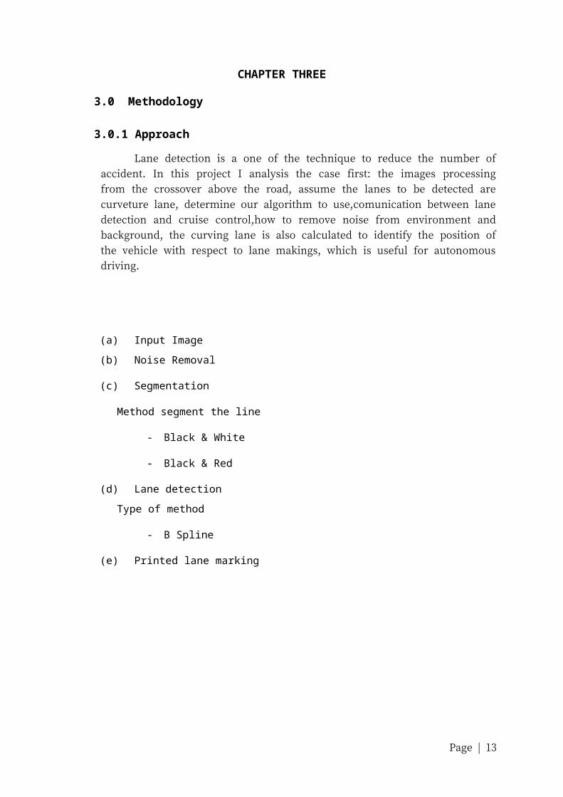
CHAPTER THREE
3.0 Methodology
3.0.1 Approach
Lane detection is a one of the technique to reduce the number of accident. In
this project I analysis the case first: the images processing from the crossover above
the road, assume the lanes to be detected are curveture lane, determine our
algorithm to use,comunication between lane detection and cruise control,how to
remove noise from environment and background, the curving lane is also calculated
to identify the position of the vehicle with respect to lane makings, which is useful for
autonomous driving.
(a) Input Image
(b) Noise Removal
(c) Segmentation
Method segment the line
- Black & White
- Black & Red
(d) Lane detection
Type of method
- B Spline
(e) Printed lane marking
Page | 11
Page | 12
(a) Input Image
At the bigining of the process,this project capture or take a vedeo an
image of the road including the road bacground at a daytime with good
weather condition. The image are capture or take vedeo by the camere locate
in front of the wind screen of the vehicle and considered the lane marking can
be solid line or dash line in different scenario of road (curved road)
(b) Removal Noise
The removal noise use the Kalman Filter base on this information and do by following this guide:-
The Kalman Filter
The Kalman filter is a computationally efficient, recursive,
discrete, linear filter.It can give estimates of past, present and future
states of a system even when the underlying model is imprecise or
unknown. For more on the Kalman filter there are many good
references available to explain it: [Welch00; Gelb74; Maybeck79]. The
two most important aspects of the Kalman algorithm are the system
model and the noise models. (Equations 1−5 describe the filter in one
common way of expressing it.)
(c) Segmentation
Page | 13

The image capture by the camera is in RGB image to convert from
original image into gray scale image.Refering the privious study,the
explaination about the convert from original image into gray scale image is:
from the converted image,all boundaries within this image are extracted by
horizontal differentation using sobel edge detector to generate the adge point.
Edge detection by far is amost common approach for detecting meaningful
discontinnuities in gray level to find the approximate absolute gradient
magnitude at each point in an input gray scale image.
After converted into gray scale,that image convert into black-white,and
black-red to show the line clearly by following this step:-
Step 1: Install Image Acquisition Device
Step 2: Retrieve Hardware Information
Step 3: Create a Video Input Object
Step 4: Preview the Video Stream (Optional)
Step 5: Configure Object Properties (Optional)
Step 6: Acquire Image Data
The segmentation steps required to create an image acquisition application by
implementing a motion and line detection application. The application detects
movement in a scene by performing a pixel-to-pixel comparison in pairs of incoming
image frames. If nothing moves in the scene, pixel values remain the same in each
frame. When something moves in the image, the application displays the pixels that
have changed values.
The example highlights how you can use the Image Acquisition Toolbox software
to create a working image acquisition application with only a few lines of code.
Step 1: Install Image Acquisition Device
Follow the setup instructions that come with image acquisition device. Setup typically
involves:
a) Installing the frame grabber board in computer.
b) Installing any software drivers required by the device. These are supplied by
the device vendor.
Page | 14

c) Connecting a camera to a connector on the frame grabber board.
d) Verifying that the camera is working properly by running the application
software that came with the camera and viewing a live video stream.
Generic Windows image acquisition devices, such as webcams and digital video
camcorders, typically do not require the installation of a frame grabber board.Connect
these devices directly to your computer via a USB or FireWire port.
After installing and configuring your image acquisition hardware, start MATLAB on your
computer by double-clicking the icon on your desktop. You do not need to perform any
special configuration of MATLAB to perform image acquisition.
Step 2: Retrieve Hardware Information
Device Information
Description
Adaptor name
An adaptor is the software that the toolbox uses to communicate with an image acquisition device via its device driver. The toolbox includes adaptors for certain vendors of image acquisition equipment and for particular classes of image acquisition devices. See Determining the Adaptor Name for more information.
Device ID The device ID is a number that the adaptor assigns to uniquely identify each image acquisition device with which it can communicate. See Determining the Device ID for more information.
Note Specifying the device ID is optional; the toolbox uses the first available device ID as the default.
Video format The video format specifies the image resolution (width and height) and other aspects of the video stream. Image acquisition devices typically support multiple video formats. See Determining the Supported Video Formats for more information.
Note Specifying the video format is optional; the toolbox uses one of the supported formats as the default.
In this step,get several pieces of information that the toolbox needs to uniquely identify
the image acquisition device want to access.
Page | 15

Page | 16
Determining the Adaptor Name
To determine the name of the adaptor, enter the imaqhwinfo function at the MATLAB prompt without any arguments.
imaqhwinfoans =
InstalledAdaptors: {'dcam' 'winvideo'} MATLABVersion: '7.4 (R2007a)' ToolboxName: 'Image Acquisition Toolbox' ToolboxVersion: '2.1 (R2007a)'

Page | 17
Determining the Device ID
To find the device ID of a particular image acquisition device, enter the imaqhwinfo function at the MATLAB prompt, specifying the name of the adaptor as the only argument. (You found the adaptor name in the first call to imaqhwinfo, described in Determining the Adaptor Name.) In the data returned, the DeviceIDs field is a cell array containing the device IDs of all the devices accessible through the specified adaptor.
Note This example uses the DCAM adaptor. Substitute the name of the adaptor would like to use.
info = imaqhwinfo('dcam')info =
AdaptorDllName: [1x77 char] AdaptorDllVersion: '2.1 (R2007a)' AdaptorName: 'dcam' DeviceIDs: {[1]}
Determining the Supported Video Formats
To determine which video formats an image acquisition device supports, look in the DeviceInfo field of the data returned by imaqhwinfo. The DeviceInfo field is a structure array where each structure provides information about a particular device. To view the device information for a particular device,can use the device ID as a reference into the structure array. Alternatively, you can view the information for a particular device by calling the imaqhwinfo function, specifying the adaptor name and device ID as arguments.
To get the list of the video formats supported by a device, look at SupportedFormats field in the device information structure. The SupportedFormats field is a cell array of strings where each string is the name of a video format supported by the device. For more information, see Determining Supported Video Formats.
dev_info = imaqhwinfo('dcam',1)
dev_info =
DefaultFormat: 'F7_Y8_1024x768' DeviceFileSupported: 0 DeviceName: 'XCD-X700 1.05' DeviceID: 1 ObjectConstructor: 'videoinput('dcam', 1)' SupportedFormats: {'F7_Y8_1024x768' 'Y8_1024x768'}

Step 3: Create a Video Input Object
In this step create the video input object that the toolbox uses to represent the
connection between MATLAB and an image acquisition device. Using the properties
of a video input object,can control many aspects of the image acquisition process. For
more information about image acquisition objects, see Connecting to Hardware.
To create a video input object, use the videoinput function at the MATLAB
prompt. The DeviceInfo structure returned by the imaqhwinfo function contains the
default videoinput function syntax for a device in the ObjectConstructor field. For
more information the device information structure, see Determining the Supported
Video Formats.
The following example creates a video input object for the DCAM adaptor.
Substitute the adaptor name of the image acquisition device available on your
system.
vid = videoinput('dcam',1,'Y8_1024x768')
The videoinput function accepts three arguments: the adaptor name, device
ID, and video format.Retrieved this information in step 2. The adaptor name is the
only required argument; the videoinput function can use defaults for the device ID and
video format. To determine the default video format, look at the Default Format field in
the device information structure. See Determining the Supported Video Formats
for more information.
Instead of specifying the video format,can optionally specify the name of a
device configuration file, also known as a camera file. Device configuration files are
typically supplied by frame grabber vendors. These files contain all the required
configuration settings to use a particular camera with the device. See Using Device
Configuration Files (Camera Files) for more information.
Viewing the Video Input Object Summary
To view a summary of the video input object you just created, enter the
variable name (vid) at the MATLAB command prompt. The summary information
displayed shows many of the characteristics of the object, such as the number of
frames that will be captured with each trigger, the trigger type, and the current state of
the object.Use video input object properties to control many of these characteristics
Page | 18

Step 4: Preview the Video Stream (Optional)
After create the video input object, MATLAB is able to access the image
acquisition device and is ready to acquire data. However, before begin,to see a
preview of the video stream to make sure that the image is satisfactory. For
example,to change the position of the camera, change the lighting, correct the focus,
or make some other change to image acquisition setup.
Note This step is optional at this point in the procedure because can preview a video
stream at any time after you create a video input object.
To preview the video stream in this example, enter the preview function at the
MATLAB prompt, specifying the video input object created in step 3 as an argument.
preview(vid)
The preview function opens a Video Preview figure window on screen containing the
live video stream. To stop the stream of live video,can call the stoppreview function.
To restart the preview stream, call preview again on the same video input object.
While a preview window is open, the video input object sets the value of the
Previewing property to 'on'. If change characteristics of the image by setting image
Page | 19
vid
Summary of Video Input Object Using 'XCD-X700 1.05'.
Acquisition Source(s): input1 is available.
Acquisition Parameters: 'input1' is the current selected source.10 frames per trigger using the selected source.
'Y8_1024x768' video data to be logged upon START. Grabbing first of every 1 frame(s). Log data to 'memory' on trigger.
Trigger Parameters: 1 'immediate' trigger(s) on START. Status: Waiting for START. 0 frames acquired since starting. 0 frames available for GETDATA.

acquisition object properties, the image displayed in the preview window reflects the
change.
Step 5: Configure Object Properties (Optional)
After creating the video input object and previewing the video stream,if want to
modify characteristics of the image or other aspects of the acquisition process.
Accomplish this by setting the values of image acquisition object properties. This
section
Describes the types of image acquisition objects used by the toolbox
Describes how to view all the properties supported by these objects, with
their current values
Describes how to set the values of object properties
Types of Image Acquisition Objects
The toolbox uses two types of objects to represent the connection with an
image acquisition device:
Video input objects
Video source objects
A video input object represents the connection between MATLAB and a video
acquisition device at a high level. The properties supported by the video input object
are the same for every type of device.Created a video input object using the
videoinput function in step 3.
Create a video input object, the toolbox automatically creates one or more
video source objects associated with the video input object. Each video source object
represents a collection of one or more physical data sources that are treated as a
single entity. The number of video source objects the toolbox creates depends on the
device and the video format specify. At any one time, only one of the video source
objects, called the selected source, can be active. This is the source used for
acquisition. For more information about these image acquisition objects, see
Creating Image Acquisition Objects.
Page | 20

Viewing Object Properties
To view a complete list of all the properties supported by a video input object
or a video source object, use the get function. To list the properties of the video input
object created in step 3, enter this code at the MATLAB prompt.
get(vid)
The get function lists all the properties of the object with their current values.
To view the properties of the currently selected video source object associated
with this video input object, use the getselectedsource function in conjunction with the
get function. The getselectedsource function returns the currently active video source.
To list the properties of the currently selected video source object associated with the
video input object created in step 3, enter this code at the MATLAB prompt.
get(getselectedsource(vid))
The get function lists all the properties of the object with their current values.
Note Video source object properties are device specific. The list of properties
supported by the device connected to system might differ from the list shown in this
example.
Page | 21
General Settings: DeviceID = 1 DiskLogger = [] DiskLoggerFrameCount = 0 EventLog = [1x0 struct] FrameGrabInterval = 1 FramesAcquired = 0 FramesAvailable = 0 FramesPerTrigger = 10 Logging = off LoggingMode = memory Name = Y8_1024x768-dcam-1 NumberOfBands = 1 Previewing = on ReturnedColorSpace = grayscale ROIPosition = [0 0 1024 768] Running = off Tag = Timeout = 10 Type = videoinput

Setting Object Properties
To set the value of a video input object property or a video source object
property,can use the set function or you can reference the object property as would a
field in a structure, using dot notation.
Some properties are read only;cannot set their values. These properties
typically provide information about the state of the object. Other properties become
read only when the object is running. To view a list of all the properties can set, use
the set function, specifying the object as the only argument.
To implement continuous image acquisition, the example sets the
TriggerRepeat property to Inf. To set this property using the set function, enter this
code at the MATLAB prompt.
set(vid,'TriggerRepeat',Inf);
To help the application keep up with the incoming video stream while
processing data, the example sets the FrameGrabInterval property to 5. This
specifies that the object acquire every fifth frame in the video stream. (need to
experiment with the value of the FrameGrabInterval property to find a value that
provides the best response with image acquisition setup.) This example shows how
can set the value of an object property by referencing the property as you would
reference a field in a MATLAB structure.
vid.FrameGrabInterval = 5;
To set the value of a video source object property,must first use the
getselectedsource function to retrieve the object. (can also get the selected source by
Page | 22
General Settings: Parent = [1x1 videoinput] Selected = on SourceName = input1 Tag = Type = videosource
Device Specific Properties: FrameRate = 15 Gain = 2048 Shutter = 2715

searching the video input object Source property for the video source object that has
the Selected property set to 'on'.)
To illustrate, the example assigns a value to the Tag property.
vid_src = getselectedsource(vid);
set(vid_src,'Tag','motion detection setup');
Step 6: Acquire Image Data
After create the video input object and configure its properties,that can acquire
data. This is typically the core of any image acquisition application, and it involves
these steps:
Starting the video input object —Start an object by calling the start
function. Starting an object prepares the object for data acquisition. For
example, starting an object locks the values of certain object properties
(they become read only). Starting an object does not initiate the acquiring
of image frames, however. The initiation of data logging depends on the
execution of a trigger.
The following example calls the start function to start the video input
object. Objects stop when they have acquired the requested number of
frames. Because the example specifies a continuous acquisition, you must
call the stop function to stop the object.
Triggering the acquisition — To acquire data, a video input object must
execute a trigger. Triggers can occur in several ways, depending on how
the TriggerType property is configured. For example, if you specify an
immediate trigger, the object executes a trigger automatically, immediately
after it starts. If you specify a manual trigger, the object waits for a call to
the trigger function before it initiates data acquisition. For more
information, see Acquiring Image Data.
In the example, because the TriggerType property is set to 'immediate'
(the default) and the TriggerRepeat property is set to Inf, the object
Page | 23

automatically begins executing triggers and acquiring frames of data,
continuously.
Bringing data into the MATLAB workspace — The toolbox stores
acquired data in a memory buffer, a disk file, or both, depending on the
value of the video input object LoggingMode property. To work with this
data,must bring it into the MATLAB workspace. To bring multiple frames
into the workspace, use the getdata function. Once the data is in the
MATLAB workspace,can manipulate it as would any other data. For more
information, see Working with Acquired Image Data.
Note The toolbox provides a convenient way to acquire a single
frame of image data that doesn't require starting or triggering the
object. See Bringing a Single Frame into the Workspace for more
information.
Running the Example
To run the example, enter the following code at the MATLAB prompt. The
example loops until a specified number of frames have been acquired. In each loop
iteration, the example calls getdata to bring the two most recent frames into the
MATLAB workspace. To detect motion, the example subtracts one frame from the
other, creating a difference image, and then displays it. Pixels that have changed
values in the acquired frames will have nonzero values in the difference image.
The getdata function removes frames from the memory buffer when it brings
them into the MATLAB workspace. It is important to move frames from the memory
buffer into the MATLAB workspace in a timely manner. If do not move the acquired
frames from memory,can quickly exhaust all the memory available on system.
Note The example uses functions in the Image Processing Toolbox software.
Page | 24

(d) Lane Detection
The lane detection use the B-Spline base on this information and do by following this guide:-
For a set of infinite data points where for any , the B-splines of
degree are defined as
(5.1.1)
and
(5.1.2)
Page | 25
% Create video input object. vid = videoinput('dcam',1,'Y8_1024x768')
% Set video input object properties for this application.% Note that example uses both SET method and dot notation method.set(vid,'TriggerRepeat',Inf);vid.FrameGrabInterval = 5;
% Set value of a video source object property.vid_src = getselectedsource(vid);set(vid_src,'Tag','motion detection setup');
% Create a figure window.figure;
% Start acquiring frames.start(vid)
% Calculate difference image and display it.while(vid.FramesAcquired<=100) % Stop after 100 frames data = getdata(vid,2); diff_im = imabsdiff(data(:,:,:,1),data(:,:,:,2)); imshow(diff_im);end
stop(vid)

x(i-1) x(i) x(i+1) x(i+2) x(i+3) x(i+4)0
0.5
1
1.5
Bi0 B
i+20
where i and k are integers as usual. Note: always.
Each is nonzero in exactly one interval (Figure 5.1.1) and has a discontinuity at
. For any dataset , the “constant” B-spline is
(5.1.3)
which simply extends each across each interval.
Page | 26

Figure 3.1.1 Non-zero parts of B-splines of degree 0.
For , can be derived from Equations 5.1.1.and 5.1.2 as
(5.1.4)
which has two non-zero parts, in intervals and as shown in
Figure 5.1.2 (Dashed lines are used in order to make the splines more distinguishable).
These intervals are called the support of . On each of its support intervals,
is a linear function and its location and slope are solely determined by the
distribution of the ’s. has a peak value of 1 at and is continuous there. It is
quite clear that has but not continuity.
Page | 27

x(i-1) x(i) x(i+1) x(i+2) x(i+3) x(i+4)0
0.5
1
1.5
Bi-11 Bi
1 Bi+11 Bi+2
1
Figure 3.1.2 Non-zero parts of B-splines of degree 1.
Page | 28

It is interesting to note that has some connection to the elementary Lagrange
interpolating polynomial. If we write the linear Lagrange interpolating polynomial for the
two-point data set of , the two elements would be:
which are the second part of and the first part of , respectively. As we shall learn, this agreement does not extend to higher order B-splines.
In general, the 1st order B-spline is constructed from
(5.1.5)
where are constants determined from the data. However, we know from Section 4.1.1 that the linear spline on a given data interval is also the Lagrange interpolation formula for the data set consisting of the two end points of the same data interval. So let’s discuss the relationship of with the linear splines. It turns out that for any
data set , the following function is a linear spline:
(5.1.6)
To prove it, let’s look at the formula of on interval . Of all the terms in the
above equation, only and have non-zero contributions on the interval. Thus
(5.1.7)
On the interval , will take the second leg of its formula and will take the first leg of its formula (see Equation 5.1.4). Thus
(5.1.8)
which is exactly the linear spline (see Equation 4.1.1) as well as the linear Lagrange interpolating polynomial.
Page | 29

Say are the only nonzero data, then
where
and
The central row is the same as a Lagrange interpolating polynomial, but in terms
of B-splines is more general: it contains Lagrange plus two arbitrary end extensions
(points are not part of the data set) as seen in Fig 5.1.3.
Now we see why we would use instead of in Equation 5.1.5 and 5.1.6.
The reason is that the hat shape of (Figure 5.1.2) is centered at , not . For
’s contribution to take place, it should be teamed with a component of B-splines
Page | 30

Figure 3.1.3 First degree B-spline for two data points.
that lags by 1. So yi is teamed with . Similar notation is used for all higher
order B-splines. For example, in the case of which will be discussed later, the
sum over of terms are used together. Furthermore, since is
centered on , . Further insight can be gleamed from Figure 5.1.2.
It is worth noting that on , + = 1 exactly. As we will prove
later, this is true for all orders of B-splines on all intervals.
Generally for linear splines, two points are used to draw a straight line for each interval. Then for each data point, its x and y information will contribute to two splines.
In the case of , this contribution is built into its expression through its two legs.
This is the essence of all B-splines and one reason why they are called “basis” splines.
Polynomial splines and Lagrange interpolating polynomials discussed before can all be viewed as functions over interval(s), as functions should be. The emphasis here is on the intervals. A polynomial is set up over the interval(s), then, we go to its end points for help on determining the coefficients of the polynomials.
B-splines, however, should be viewed more as belonging to the points. Each “point” function covers certain interval(s). To build splines through B-splines, we will always use the form similar to that in Equation 5.1.5. The y information is applied to the “point” function and we are done (almost, anyway) with the building of the splines.
This feature will be more evident in the case for .
Page | 31
00B 0
1B 02B
1
y1
y2
xx0 x1 x2 x3

(e) Printed Lane Marking Candidate Selection
Last part of this project is printed lane marking candidate selection ,this part
is to display the final result for curveture lane detection and plotting.
3.1 ANALYSIS
Refer to the our topic,this project must be identified type of method or process to put
into this project.
I. Define type of algorithm to use.
B. Snake [3]
B Snake is used in a variety of related methods for shape detection.
These methods are fairly important in applied computer vision; in fact, B
Snake published his transform in a patent application, and various later
patents are also associated with the technique. Here I use it to detect the
curveture lines.
B snake is a good approximation of the traditional snake. B snake
represent the snake compactly, allow corners, and converge fast. Thus it can
be applied instead of snake where I need efficient implementation.
B. Spline [1][2]
Besides B-Spline, other kind splines also can be used in our lane
model. Our early version of lane model used Catmull-Rom spline. The
different between the B-Spline and the other kind splines is the locations of the
control points.
[1] APPANDICES-FIGURE 1
[2] APPANDICES-FIGURE 2
[3] APPANDICES-FIGURE 1
Page | 32

3.2 EQUIPMENT AND SOFTWARE USE
This Final Year Project attemps to produce Study On Line Detection Applied On
Cruise Control System on the following equipment and software use:-
SOFTWARE : MATLAB in image processing toolbox
The study on image processing toolkit using computer language Matlab
was conducted to perform moving object detecting technical processing on
video images. First, video pre-processing steps such as frame separation,
binary operation, gray enhancement and filter operation were conducted. Then
the detection and extraction of moving object was carried out on images
according to frame difference-based dynamic-background refreshing
algorithm. Finally, the desired video image was synthesized through adding
image casing on the moving objects in the video. The results showed that
using computer language Matlab to perform moving object detecting algorithm
has favorable effects.
EQUIPMENT : Camera in USB communication cable
Page | 33

CHAPTER FOUR
4.0 EXPERIMENTAL
Several experiment which related with study was done to support and prove the result of this project:-
(a)
(b) (c)
(d) (e) (f)
(e)
Page | 34

Experimental results for lane detection:
(a) Input image
(b) Filtering Noise
(c) Second stage Filtering Noise
(d) After filtering noise
(e) Lane mapping using black and white
(f) Lane mapping using black and red
Page | 35

CHAPTER FIVE
5.0 RESULT/DISCUSION
There are several type of technique to study or produce this project.The
techniques that used in this project are noise removal,segmentation,line detection
and lane marking. Before have a result,this project have a some problem or error to
solve and the problem will be solve in several technique and step.One of the
technique is do the experiment.
This project and study more focus to image processing and related to cruse
control system and operation.Before do the project,the spec of camera must be
identify because this important to Matlab communicated beteween camera and their
software.The toolbox toidentified spec of camera is image acquisition.The tecqniue to
identify spec of camera is:-
Page | 36
The imaqhwinfo function provides a structure with an InstalledAdaptors field that lists
all adaptors on the current system that the toolbox can access.
>>imaqInfo = imaqhwinfo
imaqInfo =
InstalledAdaptors: {'coreco' 'matrox' 'winvideo'} MATLABVersion: '7.11 (R2010b)' ToolboxName: 'Image Acquisition Toolbox' ToolboxVersion: '4.0 (R2010b)'
>> imaqInfo.InstalledAdaptors
ans =
'coreco' 'matrox' 'winvideo'
Obtaining Device Information
Calling imaqhwinfo with an adaptor name returns a structure that provides information on all accessible image acquisition devices .
>> hwInfo = imaqhwinfo('winvideo')
hwInfo = AdaptorDllName: 'C:\Program Files\MATLAB\R2010b\toolbox\imaq\imaqadaptors\win32\mwwinvideoimaq.dll'
AdaptorDllVersion: '4.0 (R2010b)' AdaptorName: 'winvideo'

Page | 37
DeviceIDs: {[1]} DeviceInfo: [1x1 struct]
>> hwInfo.DeviceInfo
ans = DefaultFormat: 'YUY2_160x120'DeviceFileSupported: 0DeviceName: 'USB Video Device'DeviceID: 1ObjectConstructor: 'videoinput('winvideo', 1)'SupportedFormats: {'YUY2_160x120' 'YUY2_176x144' 'YUY2_320x240' 'YUY2_352x288' 'YUY2_640x480'}
Information on a specific device can be obtained by simply indexing into the device information structure array.>> device1 = hwInfo.DeviceInfo(1)
device1 =
DefaultFormat: 'YUY2_160x120'DeviceFileSupported: 0DeviceName: 'USB Video Device'DeviceID: 1ObjectConstructor: 'videoinput('winvideo', 1)'SupportedFormats: {'YUY2_160x120' 'YUY2_176x144' 'YUY2_320x240' 'YUY2_352x288' 'YUY2_640x480'}
The DeviceName field contains the image acquisition device name. >> device1.DeviceName
ans =
USB Video Device
The DeviceID field contains the image acquisition device identifier. >> device1.DeviceID
ans =
1
The DefaultFormat field contains the image acquisition device's default video format.>> device1.DefaultFormat
ans =
YUY2_160x120

5.1 NOISE REMOVAL
There are several technique used in filtering process. Type of the thechniques
are Midian Filter,FIR Filter,Kalman Filter, IIR Filter, Adaptive Filter and etc.In this
project, the technique used is Kalman Filter to eliminate or remove noises in the video
recorde. The celebrated Kalman filter, rooted in the state-space formulation of linear
dynamical systems, provides a recursive solution to the linear optimal filtering
problem. It applies to stationary as well as no stationary environments. The solution is
recursive in that each updated estimate of the state is computed from the previous
estimate and the new input data, so only the previous estimate requires storage. In
addition to eliminating the need for storing the entire past observed data, the Kalman
filter is computationally more efficient than computing the estimate directly from the
entire past observed data at each step of the filtering process.
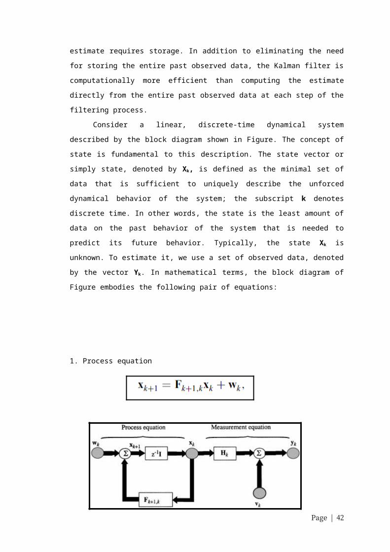
Consider a linear, discrete-time dynamical system described by the block
diagram shown in Figure. The concept of state is fundamental to this description. The
state vector or simply state, denoted by Xk, is defined as the minimal set of data that
is sufficient to uniquely describe the unforced dynamical behavior of the system; the
subscript k denotes discrete time. In other words, the state is the least amount of data
on the past behavior of the system that is needed to predict its future behavior.
Typically, the state Xk is unknown. To estimate it, we use a set of observed data,
denoted by the vector Yk. In mathematical terms, the block diagram of Figure
embodies the following pair of equations:
Page | 38
The Supported Formats field contains a cell array of all valid video formats supported by the image acquisition device.
>> device1.SupportedFormats
ans = 'YUY2_160x120' 'YUY2_176x144' 'YUY2_320x240' 'YUY2_352x288' 'YUY2_640x480'
After identified the spec of camera,the MATLAB can communicate their camera and can do several technique until end of the project.

1. Process equation
Signal-flow graph representation of a linear, discrete-time dynamical system
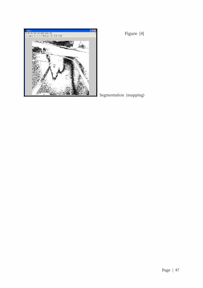
5.2 SEGMENTATION
There are several technique used in segmentation process. Type of techniques
are ROI (Region of interest) and mapping.In this project, the technique used is
mapping is seperate into two color to show the different image for exampli used black
and white mapping.[4]
[1] APPANDICES-FIGURE 4
Page | 39

5.3 LINE DETECTION
There are several algorithm used in curveture line detection. Type of
algorithm are B-Spline and B-Snake.In this project, the algorithm used is B-Spline.
The B-Spline algorithm is plotting in short distance compare with B-Snake algorithm
that used the anggle of the road for plotting the point . For read the coordinate of the
road,the value of X exist and Y exist must identified.
Example of B-Spline
[08,110] Y X
Page | 40

CHAPTER SIX
CONCLUSION AND FUTURE WORK
Lane detection and tracking plays a significant role in driver assistance
systems (DAS) since the 1990s. The first lane departure warning system was available
in a 1995 Mitsubishi Diamante. It is commonly used in trucks since about 2000, when it
became standard in Mercedes trucks. It proves to be very useful on highways or other
roads with clearly marked lanes. However, lane detection and tracking is still (2009) a
challenge when roads are narrow, windy, with incomplete lane markings, hidden lane
markings due to parked cars or shadows, and other situations. Lane detection tracking
is used in intelligent cruise control systems, typically for lane departure warning, but
also has relevance for road modeling or other more advanced tasks.
For the conclusion, there is having much technique in image processing to
identify and applied into our project but must be know what the term of image
processing are used. In coming soon project hope this project can upgrade into
developed the hardware part and can combine between image processing and cruise
control system.
Page | 41
APPANDICES
Figure [1]
B-spline model represents midline of the road.
Figure [2]
Normals on B-spline model for feature extraction.
Figure [3]
B-Snake based lane model
Page | 42

Figure [4]
Segmentation (mapping)
Page | 43

SOURCE CODE
% Access an image acquisition device.vidobj = videoinput('winvideo');% Convert the input images to rgb.set(vidobj, 'ReturnedColorSpace', 'rgb')% Retrieve the video resolution.vidRes = get(vidobj, 'VideoResolution');Imfilter = vidRes/4[MR,MC,Dim] = size(Imfilter);% Create a figure and an image object.f = figure('Visible', 'off');% The Video Resolution property returns values as width by height, but% MATLAB images are height by width, so flip the values.imageRes = fliplr(Imfilter); subplot(1,1,1);hImage = imshow(zeros(imageRes));% The PREVIEW function starts the camera and display. The image on which to% display the video feed is also specified.preview(vidobj, hImage);pause(5);% Convert the input images to grayscale.set(vidobj, 'ReturnedColorSpace', 'grayscale')% View the vedeo for 5 seconds.pause(5);stoppreview(vidobj); delete(f); % Access an image acquisition device.vidobj = videoinput('winvideo');% Convert the input images to grayscale.set(vidobj, 'ReturnedColorSpace', 'grayscale')% Retrieve the video resolution.vidRes = get(vidobj, 'VideoResolution');Imfilter = vidRes/2[MR,MC,Dim] = size(Imfilter);% Create a figure and an image object.f = figure('Visible', 'off');% The Video Resolution property returns values as width by height, but% MATLAB images are height by width, so flip the values.imageRes = fliplr(Imfilter); subplot(1,1,1);hImage = imshow(zeros(imageRes));% The PREVIEW function starts the camera and display. The image on which to% display the video feed is also specified.preview(vidobj, hImage);% View the vedeo for 5 seconds.pause(2);stoppreview(vidobj); delete(f); % Access an image acquisition device.vidobj = videoinput('winvideo');% Convert the input images to grayscale.set(vidobj, 'ReturnedColorSpace', 'grayscale')% Retrieve the video resolution.vidRes = get(vidobj, 'VideoResolution');Imfilter = vidRes/1[MR,MC,Dim] = size(Imfilter);% Create a figure and an image object.f = figure('Visible', 'off');
Page | 44

% The Video Resolution property returns values as width by height, but% MATLAB images are height by width, so flip the values.imageRes = fliplr(Imfilter); subplot(1,1,1);hImage = imshow(zeros(imageRes));% The PREVIEW function starts the camera and display. The image on which to% display the video feed is also specified.preview(vidobj, hImage);% View the vedeo for 5 seconds.pause(5);% Convert the input images to rgb.set(vidobj, 'ReturnedColorSpace', 'rgb')% View the vedeo for 5 seconds.pause(5);stoppreview(vidobj); delete(f); % Create video input object. vid = videoinput('winvideo',1,'YUY2_640x480') % Set video input object properties for this application.% Note that example uses both SET method and dot notation method.set(vid,'TriggerRepeat',Inf);vid.FrameGrabInterval = 8; % Set value of a video source object property.vid_src = getselectedsource(vid);set(vid_src,'Tag','motion detection setup'); % Create a figure window.figure; % Start acquiring frames.start(vid)% Calculate difference image and display it.while(vid.FramesAcquired<=10) % Stop after 100 frames data = getdata(vid,2); diff_im1 = imabsdiff(data(:,:,1),data(:,:,2)); diff_im2 = imabsdiff(data(:,:,1),data(:,:,3)); I= diff_im1.* diff_im2; imshow(I);endpause(1); while(vid.FramesAcquired<=40) % Stop after 100 frames data = getdata(vid,2); diff_im3 = imabsdiff(data(:,:,1),data(:,:,3)); diff_im4 = imabsdiff(data(:,:,2),data(:,:,1)); I= diff_im3.* diff_im4; imshow(I);endpause(1); % Calculate difference image and display it.while(vid.FramesAcquired<=50) % Stop after 100 frames data = getdata(vid,2); diff_im = imabsdiff(data(:,:,:,1),data(:,:,:,2)); imshow(diff_im);endstop(vid)delete(vid)clear
Page | 45

close(gcf) % Access an image acquisition device.vidobj = videoinput('winvideo');% Convert the input images to rgb.set(vidobj, 'ReturnedColorSpace', 'rgb')% Retrieve the video resolution.vidRes = get(vidobj, 'VideoResolution');Imfilter = vidRes/1 [MR,MC,Dim] = size(Imfilter);% Create a figure and an image object.f = figure('Visible', 'off');% The Video Resolution property returns values as width by height, but% MATLAB images are height by width, so flip the values.imageRes = fliplr(Imfilter); subplot(1,1,1);hold on;npts = 1;xy = [randn(1,npts); randn(1,npts)];hImage = imshow(zeros(imageRes)),text(17,110,'Line Detection Applied On Cruise Control By Kasran','Color','b','BackgroundColor',[.7 .9 .7],... 'FontWeight', 'bold');% The PREVIEW function starts the camera and display. The image on which to% display the video feed is also specified.preview(vidobj, hImage);pause (0.5);imshow1=plot(08,110,'r*','Color',[1 0 0]);imshow9=plot(159,104,'r*','Color',[1 0 0]);pause (0.5);imshow2=plot(14,103,'r*','Color',[1 0 0]);imshow10=plot(156,97,'r*','Color',[1 0 0]);pause(0.5);imshow3=plot(20,96,'r*','Color',[1 0 0]); imshow11=plot(152,90,'r*','Color',[1 0 0]);pause(0.5);imshow4=plot(26,89,'r*','Color',[1 0 0]);imshow12=plot(147,83,'r*','Color',[1 0 0]);pause(0.5);imshow5=plot(32,82,'r*','Color',[1 0 0]);imshow13=plot(144,76,'r*','Color',[1 0 0]);pause(0.5);imshow6=plot(38,75,'r*','Color',[1 0 0]);imshow14=plot(140,69,'r*','Color',[1 0 0]);pause(0.5)imshow7=plot(44,68,'r*','Color',[1 0 0]);imshow15=plot(134,62,'r*','Color',[1 0 0]);pause(0.5)imshow8=plot(50,61,'r*','Color',[1 0 0]);imshow16=plot(128,55,'r*','Color',[1 0 0]);pause(0.5)imshow19=plot(56,54,'r*','Color',[1 0 0]);imshow20=plot(121,48,'r*','Color',[1 0 0]);pause(0.5)imshow21=plot(51,47,'r*','Color',[1 0 0]);imshow22=plot(114,41,'r*','Color',[1 0 0]);pause(0.5)imshow23=plot(46,47,'r*','Color',[1 0 0]);imshow24=plot(101,37,'r*','Color',[1 0 0]);pause(0.5)imshow25=plot(41,45,'r*','Color',[1 0 0]);imshow26=plot(88,34,'r*','Color',[1 0 0]);
Page | 46
pause(0.5)imshow27=plot(36,45,'r*','Color',[1 0 0]);imshow28=plot(80,32,'r*','Color',[1 0 0]);pause(0.5)imshow29=plot(31,45,'r*','Color',[1 0 0]);pause(0.5)imshow30=plot(26,45,'r*','Color',[1 0 0]);pause(0.5)imshow31=plot(21,45,'r*','Color',[1 0 0]);pause(0.5)imshow32=plot(16,45,'r*','Color',[1 0 0]);pause(0.5)imshow33=plot(11,45,'r*','Color',[1 0 0]);pause(0.5)imshow34=plot(06,45,'r*','Color',[1 0 0]);pause(0.5)imshow35=plot(01,45,'r*','Color',[1 0 0]);pause(0.5)imshow36=plot(00,45,'r*','Color',[1 0 0]);pause(10)delete(imshow1);delete(imshow9);pause(0.1);delete(imshow2);delete(imshow10);pause(0.1);delete(imshow3);delete(imshow11);pause(0.1);delete(imshow4);delete(imshow12);pause(0.1);delete(imshow5);delete(imshow13);pause(0.1);delete(imshow6);delete(imshow14);pause(0.1);delete(imshow7);delete(imshow15);pause(0.1);delete(imshow8);delete(imshow16);pause(0.1);delete(imshow19);delete(imshow20);pause(0.1);delete(imshow21);delete(imshow22);pause(0.1);delete(imshow23);delete(imshow24);pause(0.1);delete(imshow25);delete(imshow26);pause(0.1);delete(imshow27);delete(imshow28);pause(0.1);delete(imshow29);pause(0.1);
Page | 47

delete(imshow30);pause(0.1);delete(imshow31);pause(0.1);delete(imshow32);pause(0.1);delete(imshow33);pause(0.1);delete(imshow34);pause(0.1);delete(imshow35);pause(0.1);delete(imshow36);
Page | 48

REFRENCE
1-Lane Detection on Autonomous Vehicle--Norzalina Othman: Universiti Kuala Lumpur-Malaysian Spanish Institute
2- Lane detection and tracking using B-Snake :Yue Wanga, Eam Khwang Teoha,*, Dinggang Shenb “” -17 July 2002
3- "GOLD: A parallel real-time stereo vision system for generic obstacle and lane detection", IEEE Transaction on image processing, Vol.7, N°1M.- BERTOZZI and A. BROGGI -, January 1998.
4-A lane detection vision module for driver assistance” CH [email protected]
Kristijan Maˇcek EPF Lausanne
5-A lane detection vision module for driver assistance-Kristijan Maˇcek, Brian Williams,
Sascha Kolski, Roland Siegwart
6-Kalman Filtering-Dan Simon
7-Improvement of Adaptive Cruise Control Performance-Shigeharu Miyata,Takashi Nakagami,Sei Kobayashi,Tomoji Izumi,Hisayoshi Naito, Akira Yanou, Hitomi Nakamura, and Shin Takehara1
8- Lane Detection Using B-snake-Yue Wang, Eam Khwang and Dinggang Shen: School of Electrical and Electronic Engineering Nayang Technological University, Nayang Avenue Singapore 639798
9-Colour Image Segmentation Using the Relative Values of RGB- CHIUNHSIUN LIN: National Taipei University 69 Sec. 2 Chian_Kwo N. Road, Taipei, Taiwan, 10433 TAIWAN
10- Study on the Lane Mark Identification Method in Intelligent Vehicle Navigation- Gaoying Zhi & Wencheng Guo: College of Computer and Automatization: Tianjin Polytechnic University Tianjin 300160, China
Page | 49