sub-task no. 3 - groundwater numerical model...
TRANSCRIPT

ASR Test Well Work Plan and Model Data Collection
Contract No. W912EP-05-D-0004Delivery Order No. 1
Sub-Task No. 3 - GroundwaterNumerical Model Development
Support and Data Collection Report
Prepared for
U.S. Army Corps of Engineers,Jacksonville District
Submitted by:
4350 W. Cypress St., Ste. 600.Tampa, FL 33607
December 2005(Final-Revised July 2006)
TPA/053320001/REPORT_SUB-TASK3 TM MODEL REVIEW AND DEVELOPMENT_REV1 07_2006.DOC II
Contents
Section PageList of Acronyms......................................................................................................................... iv
Executive Summary............................................................................................................... ES-1
1 Introduction.................................................................................................................. 1-1
2 Hydrogeologic Framework Document Review ..................................................... 2-12.1 Hydrostratigraphic Units .................................................................................. 2-2
2.1.1 Upper Floridan Aquifer..................................................................... 2-22.1.2 Middle Floridan Aquifer ................................................................... 2-3
2.1.3 Lower Floridan Aquifer..................................................................... 2-4
2.1.4 Boulder Zone....................................................................................... 2-52.2 Confining Units................................................................................................... 2-5
3 Numerical Model Review.......................................................................................... 3-13.1 Southwest Florida Region Model Review....................................................... 3-1
3.1.1 Peninsular Model (Sepulveda, 2002) ............................................... 3-23.1.2 Southern District Model (Beach and Chan, 2003).......................... 3-3
3.1.3 Eastern Tampa Bay Model (Barcelo and Basso, 1993)................... 3-3
3.1.4 HydroGeoLogic Model (HydroGeoLogic, 2002) ........................... 3-4
3.1.5 SWFWMD District Wide Regulatory Model (ESI, 2004)............... 3-53.2 Comparison of Southwest Group of Models .................................................. 3-6
3.3 Southeast Florida Region Model Review........................................................ 3-8
3.3.1 Lee County Model (Bower et al., 1990) ........................................... 3-93.3.2 Lower East Coast Floridan Aquifer Model (Fairbank et al.,
1999) ..................................................................................................... 3-9
3.3.3 East-Central Floridan Aquifer Model (McGurk andPresley, 2002)....................................................................................... 3-9
3.4 Comparison of Southeast Group of Models ................................................. 3-10
4 Dispersion Research and Database.......................................................................... 4-1
5 Conceptual CERP Model Recommendations......................................................... 5-1
5.1 Common Hydrogeologic Framework.............................................................. 5-15.2 Potential ASR Storage Zones............................................................................. 5-1
5.3 Discussion of Model Framework ..................................................................... 5-2
5.3.1 SAS ....................................................................................................... 5-25.3.2 Confining and Semi-confining Units............................................... 5-2
5.3.3 Intermediate Aquifer System............................................................ 5-3
5.3.4 Upper Floridan Aquifer..................................................................... 5-3
5.3.5 Middle Floridan Aquifer and Lower Floridan Aquifer ................ 5-45.4 Discussion of Model Grid or Mesh Spacings.................................................. 5-5

TPA/053320001/REPORT_SUB-TASK3 TM MODEL REVIEW AND DEVELOPMENT_REV1 07_2006.DOC III
6 Recommended CERP Model Framework ............................................................... 6-1
7 References..................................................................................................................... 7-1
List of Appendices
Appendix A Southwest Florida Region Model Review TM
Appendix B Southeast Florida Region Model Review TMAppendix C Dispersion Database TM
List of Tables
Number
1 Groundwater Models Available for Review2 Groundwater Model Layer Comparisons
List of Figures
Number
1 Reviewed Model Boundaries
2 Wells Considered for the Hydrogeologic Framework
3 Relationship of Hydrogeologic Units Proposed by the Preliminary Hydrogeologic
Framework Study

TPA/053320001/REPORT_SUB-TASK3 TM MODEL REVIEW AND DEVELOPMENT_REV1 07_2006.DOC IV
List of Acronyms
APT Aquifer Performance Test
ASR Aquifer Storage and Recovery
BZ Boulder ZoneCERP Comprehensive Everglades Restoration Project
DWRM District Wide Regulation Model
EC East-CentralETB Eastern Tampa Bay
FAS Floridan Aquifer System
ft/day Feet per dayft2/d Square feet per day
GLAUC Glauconite marker
IAS Intermediate Aquifer SystemICU Intermediate Confining Unit
Kv Vertical hydraulic conductivity
LEC Lower East CoastLFA Lower Floridan Aquifer
LPZ Lower permeable zone
LTA Lower Tamiami AquiferMAP Middle Avon Park
MCU Middle confining unit
MFA Middle Floridan aquifermg/L Milligrams per liter
MSCU Middle semiconfining unit
SAS Surficial Aquifer SystemSD Southern District
SFWMD South Florida Water Management District
SJRWMD St. Johns River Water Management DistrictSWFWMD Southwest Florida Water Management District
SWUCA Southern Water Use Caution Area
TDS Total dissolved solidsTMR Telescopic mesh refinement
UFA Upper Florida Aquifer
UPZ Upper permeable zoneUSACE U.S. Army Corps of Engineers
USGS United States Geological Survey
TPA/053320001/REPORT_SUB-TASK3 TM MODEL REVIEW AND DEVELOPMENT_REV1 07_2006.DOC ES-1
Executive Summary
This report has been prepared for the U.S. Army Corps of Engineers (USACE) to convey the
results of a technical review of numerical groundwater models, a review of the Preliminary
Hydrogeologic Framework document, and a carbonate aquifer dispersion database study insupport of the Comprehensive Everglades Restoration Project (CERP).
A document entitled Preliminary Hydrogeologic Framework, October 4, 2004, is an interim work
product for the Aquifer Storage and Recovery (ASR) Regional Study. The report synthesizedmajor regional works on the Floridan aquifer system (FAS) into a single comprehensive
view of the hydrostratigraphy and hydraulic properties of the FAS from Orlando to Key
West. It included 770 hydrostratigraphic picks from 392 wells. Eight cross sections wereprepared from wells located in central to south Florida that had appropriate drilled depths
and adequate geophysical logs for the purpose of this study. This document proposed the
addition of a new informal aquifer, the middle Floridan Aquifer (MFA), which correlateswith regionally identifiable permeable zones.
The USACE selected eight models from a list of 32 models submitted by CH2MHILL. The
selected models provided an adequate coverage of the area of interest between Orlando andthe Florida Keys. The models were evaluated and summarized for general areas
corresponding approximately to the northern and southern regions of the Florida peninsula.
Model similarities and differences were described. In addition, the models were comparedto the hydrogeologic framework previously established through other studies conducted by
the USACE, the South Florida Water Management District (SFWMD), and the United States
Geological Survey (USGS). None of the models reviewed explicitly identified the proposedMFA.
As stated previously, a dispersion research study was conducted under the Subtask 3 scope
of work for the USACE. The goal of this research effort was to provide dispersion data fromsandstone and carbonate aquifers with a focus on technical sources from Florida and other
similar geologic environments from the United States and the world. Based on the USACE’s
scope of work, technical papers, reports and other sources available to and obtained byCH2MHILL were reviewed and dispersion values were tabulated. In addition to the
dispersion data, which were typically presented as longitudinal dispersivity, other pertinent
information (where available)was also tabulated in the database for comparative purposes.These supplemental aquifer data include transmissivity, storativity, transverse dispersivity,
molecular dispersivity, and aquifer name, matrix, thickness, and type.
Based on the data reviewed, CH2M HILL recommends construction of a 12-layer model tobe run using finite-element groundwater modeling software. Of these 12 layers, six layers
will be used to simulate permeable zones. Three of these zones are identified to be studied
further for development of potential ASR systems.
TPA/053320001/REPORT_SUB-TASK3 TM MODEL REVIEW AND DEVELOPMENT_REV1 07_2006.DOC 1-1
SECTION 1
Introduction
This report has been prepared for the U.S. Army Corps of Engineers (USACE) Jacksonville
District and the South Florida Water Management District (SFWMD) in support of the
Comprehensive Everglades Restoration Project (CERP). The scope of work for this report isbased on Subtask 3 of the Aquifer Storage and Recovery (ASR) Test Well Work Plan
Development and Model Data Collection (revised June 10, 2005; Contract No. W912EP-05-
D-004). The final purpose of the study is to provide the USACE a baseline of conceptualmodel recommendations to build an initial Florida Peninsular model. This tool will be used
to model the potential regional effects and aquifer behaviors of the CERP ASR
implementation plan.
The purpose of this report is to convey the results of a technical review of eight numerical
groundwater models selected by the USACE and compare this information to the known
hydrogeology of Florida. The eight models were selected by the USACE from a list of 32models prepared by CH2MHILL. Table 1 provides the list of models. The selected models
provided an adequate coverage of the area of interest between Orlando and the Florida
Keys. The model review areas correspond to the northern and southern regions of Florida,which are generally north or south of Lake Okeechobee, as shown on Figure 1. The reviews
describe the similarities and differences between these models, both individually and
regionally, and provide key information for USACE’s consideration for future developmentof a peninsula-wide groundwater numerical model from Orlando to the Florida Keys.
Table 2 presents a comparison of the reviewed groundwater model layering schemes.
Recommendations on numerical model layering are provided in this report based on themodel reviews included inAppendices A and B of this report with comparison to the Draft-
Final Report -Task 3.0. Define Preliminary Hydrogeologic Framework, October 4, 2004, prepared
by Ron Reese (USGS – Project lead) and Emily Richardson (SFWMD– Task lead).
Within Subtask 3, the USACE required the development of a groundwater dispersion
database. A separate TM has been prepared and is included in Appendix C to document the
results of a literature search and development of the groundwater dispersion database. Thegoal of this research is to provide dispersion data on primarily sandstone and carbonate
aquifers with a focus on technical sources from Florida and other similar geologic
environments from the United States and the world.
TPA/053320001/REPORT_SUB-TASK3 TM MODEL REVIEW AND DEVELOPMENT_REV1 07_2006.DOC 2-1
SECTION 2
Hydrogeologic Framework Document Review
Prepared by the USGS with assistance from the SFWMD, theDraft-Final Report -Task 3.0.
Define Preliminary Hydrogeologic Framework, October 4, 2004, is an interim work product for
the ASR Regional Study. The report synthesized major regional works on the Floridanaquifer system (FAS) into a single comprehensive view of the hydrostratigraphy and
hydraulic properties of the FAS from Orlando to Key West. It included 770
hydrostratigraphic picks from 392 wells. Figure 2 presents the wells reviewed for thishydrogeological framework study. The sources of information evaluated through the study
are included in Section 7, References.
The framework report provides a starting point for development of a hydrologic model ofthe FAS to plan, predict, and evaluate the potential impacts of future CERP ASR
implementation. The objectives of the report were to:
1. Identify the differences in aquifer nomenclature and interpretation across the studyarea.
2. Establish stratigraphic framework through correlation of geophysical logs from key
wells.
3. Correlate major aquifers and confining units, north to south, and east to west, across
the study area.
4. Map bounding surfaces (top and bottom) of each hydrostratigraphic unit.
5. Classify available hydraulic parameter data according to the identified
hydrostratigraphic units.
6. Map transmissivity and storativity for permeable zones, and vertical hydraulicconductivity for confining units
The interpretation of data assumed that the aquifers were continuous even though there
appeared to be some question regarding correlation and aquifer continuity between points.For aquifer model development, a similar approach was recommended, but applying more
conservative approaches in areas of greater uncertainty.
The report proposed the inclusion of a new informal hydrogeologic unit for the FAS, the“middle Floridan aquifer” (MFA). The report concluded that theMFA is regionally
continuous, present above the Middle Avon Park (MAP) marker bed, that the permeability
is associated with fractured dolostone within the Avon Park Formation (but may not beequally developed across the study area), and that the MFA lies below the 10,000 milligrams
per liter (mg/L) total dissolved solids (TDS) salinity boundary in parts of the SWFWMD
area. Figure 3 shows the relationship of the hydrogeologic units evaluated and theincorporation of the proposed MFA.

TPA/053320001/REPORT_SUB-TASK3 TM MODEL REVIEW AND DEVELOPMENT_REV1 07_2006.DOC 2-2
The report identified several issues that may require additional resolution. These issueswere:
1. Confinement between the MFA and Lower Floridan Aquifer (LFA) permeable zones
as mapped in this study could be poor in some areas of southern Florida.
2. In the western portion of the study area, particularly along the coast, the “Ocala
Limestone-Avon Park Formation moderately permeable zone” was identified to have
high transmissivity locally, and is used for injection of treatedwastewater. In the study,the zone was often not includedwithin theMFA, but rather was included in the
confining unit between the Upper Florida Aquifer (UFA) and the MFA. The UFA
extends only down to the top of or into the upper part of the Ocala Limestone in thisarea. However, in other areas of the state, treated wastewater injection activities are
typically conducted in the Boulder Zone, where present, or in portions of the LF1 where
seawater exists.
3. Confinement between the UFA and MFA as mapped in this study could be poor in
some areas of north-central and northeast Florida, especially in the area of the upper
Kissimmee River Basin.
4. In the lower west coast area of the peninsula (i.e., Lee, Hendry, and Collier Counties),
the elevation of the top of the UFA exhibits considerable variability with many
pronounced high and low areas. Development of a map showing the thickness of thebasal portion of the Hawthorn Group included in the UFA was recommended as a
future task to identify the variations in the elevation.
5. The scale of the project necessitated that the Intermediate Confining Unit (ICU) orIntermediate Aquifer System (IAS) be mapped as a single unit, but they may contain
significant aquifers within much of the study area, particularly along the west coast
of the peninsula.
2.1 Hydrostratigraphic Units
As previously shown in Figure 3, the FAS is comprised of two major aquifers, the UFA and
LFA, which are separated by the Middle Confining Unit (MCU). The MCU is also known asMC1 as defined by Reese (2004). Within the UFA and LFA are significant permeable zones
such as the Lower Hawthorn Producing Zone, the MFA, and the Boulder Zone (BZ). The
following paragraphs describe the characteristics of each of these units as defined by Reese(2004).
2.1.1 Upper Floridan Aquifer
Good confinement is exhibited above the UFA as noted by artesian pressure. During
drilling, lost-circulation zones or sudden increases in the rate of penetration often help todefine the top of the UFA. However, smaller flow zones can occur above the large flow zone
near the top of the UFA, but may not be included in the UFA due to their head,
permeability, and position (thickness and degree of confinement provided by the unitseparating them from the main flow zone). The top of the UFA often coincides with a
formation boundary, but can occur over a wide range within the geologic section (e.g., from
TPA/053320001/REPORT_SUB-TASK3 TM MODEL REVIEW AND DEVELOPMENT_REV1 07_2006.DOC 2-3
within the lower part of the Hawthorn Group in southwest Florida to the upper part of the
Avon Park Formation).
The base of the UFA or top of the MCU (MC1) can be gradational and difficult to define. The
base of the UFA often occurs in the Avon Park Formation, but in the western part of the
peninsula it commonly occurs near the top of the Ocala Limestone. In order to fill somelarge data gaps in the Southwest Florida Water Management District (SWFWMD), the
elevation of the top of the Ocala Limestone was used as a surrogate for the top of the MCU
in 47 wells evaluated in the study.
South of Lake Okeechobee, there is a notable lack of fully penetrating tests in the UFA
primarily resulting from poor water quality and the development of the Surficial Aquifer
System (SAS) or IAS in this area. In the lower west coast region, there are no fullypenetrating tests south of the Caloosahatchee River. Similarly, eastward from Orlando, in
the far northeastern portion of the study area, a rapid decline in water quality has
discouraged development and therefore testing in the FAS.
Transmissivity (T) in the UFA decreases from coastal areas inland with an area of low T
extending down the center of the peninsula from southern central Florida (T less than
5,000 square feet per day [ft2/d]) to central southern Florida (T less than 15,000 ft2/d). T in 4coastal areas (Lee,Miami-Dade, St. Lucie-Martin, and Pinellas Counties) and in Orange
County reaches 50,000 ft2/d or greater. The area with highest T (greater than 50,000 ft2/d
and up to 100,000 ft2/d) extends from Pinellas County inland across northeastern ManateeCounty and into northwestern Polk County.
Measured storativity values from 82 Aquifer Performance Tests (APTs) evaluated in the
study from the UFA ranged from a low of 4.5x10⁻⁸ to a high of 0.4. Erroneously highestimates of storativity for highly anisotropic media (e.g., most flow from fractured rock,
cavernous zones, or narrow bedding plane flow zones) in the very high transmissivity areas
may be an artifact of the standard curve matching procedure for APT analysis. Erroneousestimation of storativity is likely due to high flow zones in the fractured or cavernous
intervals that violate the assumption of radial flow to the well bore.
2.1.2 Middle Floridan Aquifer
The MFA usually occurs within a thick section of the Avon Park Formation composedprimarily of dolomitic limestone and sucrosic dolomite. The permeability in theMFA is
primarily associated with fracturing, but cavernous permeability can also be present. Lost
circulation zones encountered while drilling often marks theMFA. The thickness of theMFA is commonly 300 or 400 feet, but it can be as thick as 500 or 600 feet. It reduces to 50
feet thick or less in the lower southwest Florida area.
Permeability in the MFA appears to decline abruptly south of Lake Okeechobee. The MFAhas not been extensively evaluated south of Lake Okeechobee. The report indicated that it is
particularly important to have values in this area because the closest measured values north
of the Caloosahatchee River were very high.
In general, transmissivity in theMFA has higher values than in the UFA, and has a T of
more than 200,000 ft2/d in four areas. Transmissivity is minimal (less than 5,000 ft2/d) in
most of southern Florida (south and west of Palm Beach County). The area with highest T is

TPA/053320001/REPORT_SUB-TASK3 TM MODEL REVIEW AND DEVELOPMENT_REV1 07_2006.DOC 2-4
in southwestern Florida, centered on a well in southern Desoto County (ROMP 12), where a
T of 1,600,000 ft2/d was reported. In Pinellas County, transmissivity was recorded as high as1,200,000 ft2/d.
Elimination of extreme values and partially penetrating tests left only 14 data points on
which to base storativity. Unlike the UFA, the range and distribution of estimatedstorativity in the MFA exhibits significant difference between fully penetrating and partially
penetrating tests. The highest permeability in the MFA is associated with a horizon of
fractured dolomite. Erroneous estimation of storativity is likely due to high flow zones thatviolate the assumption of radial flow to the well bore (as previously noted).
2.1.3 Lower Floridan Aquifer
The uppermost permeable zone of the LFA (LF1 as defined by Reese, 2004) is defined as the
first major permeable zone developed below the MAP marker, but above the glauconitemarker (GLAUC) near the top of the Oldsmar Formation. LF1 occurs in the lower part of the
Avon Park Formation in fractured dolostone, but tends to be more dense and massive. In
some cases, theMFA and LF1 may be separated by only a thin but apparently unfractureddolostone unit, and confinement between theMFA and LF1 may not exist in some areas.
Confinement can be very good in central and southwest Florida due to the occurrence of
pore-filling anhydrite and gypsum.
Outside of greater metropolitan Orlando, where the LF1 is highly utilized for water supply,
it is not possible to map the hydraulic properties of this zone with confidence. In Orange
and Osceola Counties, transmissivity ranges from a low of 82,000 ft2/d to a high of688,000 ft2/d. East of this area, water quality deteriorates rapidly and the LF1 is generally
greater than 10,000 mg/LTDS. As a result, the LF1 production capability has not been
tested in this area.
LF1 appears to thin significantly toward the coast in much of the study area. Model derived
values for transmissivity of the LFA exhibited a similar eastward decline and a
transmissivity of 1,360 ft2/d was estimated at well BR1217. In general, transmissivity in LF1is higher in southern Florida (greater than 80,000 ft2/d). Transmissivity greater than
100,000 ft2/d and up to almost 700,000 ft2/d occurs in north-central Florida, centered in
northwest Osceola and Orange Counties.
Geophysical logs from the Polk City core hole (POLKC 3_G) and Kaiser injection well
(W-11424) in Polk County show little evidence of the high permeability exhibited in the LF
(west of Osceola and central Orange County). Lithologic logs from both wells indicated thepresence anhydrite infilling of pore spaces and it is assumed there is little to no permeability
from that point down to the base of the FAS.
The report indicated that there are no aquifer performance tests in LF1 in southwest Florida(Lee, Collier, Glades, or Hendry Counties). Transmissivity was estimated at a number of
wells in the SWFWMD based on the aquifer thickness, from the hydrostratigraphic surfaces
generated in this study, and a hydraulic conductivity of 9.6 feet per day (ft/day) (asobserved at the South Cross Bayou Injection well, W-17073). The report concluded that there
was strong evidence to support poor to non-existent development of permeability in the
LFA in SWFWMD, but southward, the LF1 is highly permeable based on observed drillingresponse, lithologic and geophysical logs. At the South Bay site, the results of an APT of LF1
TPA/053320001/REPORT_SUB-TASK3 TM MODEL REVIEW AND DEVELOPMENT_REV1 07_2006.DOC 2-5
(72 percent of the permeable zone tested) on the southern end of Lake Okeechobee
produced a transmissivity value of almost 70,000 ft2/d.
There are only two archived values of storativity in LF1 within the DBHYDRO database,
with values of 1.2x10⁻⁵ and 2.6x10⁻⁵. In the absence of additional data, use of an average
value of 2x10⁻³ was recommended.
2.1.4 Boulder Zone
The top of BZ, a zone of very high permeability in the lower part of the LFA, was also
mapped in this study. The top of the BZ generally occurs one to several hundred feet below
the GLAUCmarker in the Oldsmar Formation, although there are some exceptions wherethe top is slightly above the marker. The BZ is not present in central Florida (north of Lee,
Glades, and Okeechobee Counties in central Florida) except along the east coast. Similar to
the uppermost permeable zone of the LFA, this zone is not developed along the coast in thenorthwest portion of the study area. BZ permeability ranges from fractured to cavernous,
and both fractured limestone and dolostone can be present. Transmissivity for the BZ is in
the order of 106 to 107 ft2/d.
2.2 Confining Units
Three confining units were identified: the Middle Confining Unit 1 (MC1), the Middle
Confining Unit 2 (MC2) and the Lower Confining Unit (LC). The report provided verticalhydraulic conductivity (Kv) data based on hydraulic well tests of confining units, leakance
values determined from hydraulic well test of aquifers and core analysis data.
The MC1 separates the UFA and MFA permeable zones. Kv of MC1 increases from the westcoast, where it is approximately 0.1 ft/day or less, to the east coast, where it is greater than
1.0 ft/day, but less than 10 ft/day. The wells with core data in MC1 were very limited and
were located primarily in the western portion of the peninsula. The MC2 separates the MFAfrom the LFA permeable zones; Kv is lowest along both the east, and west coasts of Florida.
Kv values range from less than 0.1 ft/day down to 0.01 ft/day. The LC separates LF1 from
the BZ. Kv along the east coast of Florida is generally less than 0.1 ft/day and the data arepoorly distributed.

TPA/053320001/REPORT_SUB-TASK3 TM MODEL REVIEW AND DEVELOPMENT_REV1 07_2006.DOC 3-1
SECTION 3
Numerical Model Review
Research was conducted to determine what models were available for review. The
government agencies that assisted in providing information on available models were
USACE, SWFWMD, St. Johns River Water Management District (SJRWMD), SFWMD, andUSGS. A number of engineering consultant models were previously known or recently
identified.Most, however, were not considered for placement on the list because these types
of models typically are limited in hydrogeologic calibration outside of study area; limited ingeological layering accuracy on a regional scale; and in most cases have not been subject to
regulatory peer review. For these reasons, only published models, which were constructed
by or for governmental agencies, were listed. The following eight models were selected bythe USACE for review from among 32 available models:
Eastern Tampa Bay Model (Barcelo and Basso, 1993)
Lee County Model (Bower, et al., 1990)
Lower East Coast Model (Fairbank, et al., 1999)
Peninsular Florida Model (Sepulveda, 2002)
Southern District Model (Beach and Chan, 2003)
East-Central Model (McGurk and Presley, 2002)
HydroGeoLogic Model (HydroGeoLogic, 2002)
SWFWMD District Wide Regulatory Model (ESI, 2004)
The models were divided into two groups for review. The first group included the
southwest Florida area. The second model review group included the southeast Florida
area. This grouping allowed for better model comparisons in similar areas. These modelareas were also compared to the Draft-Final Report -Task 3.0. Define Preliminary Hydrogeologic
Framework, October 4, 2004 document to determine how the model layering compared to
actual field information. Two model review TMs were produced, one each for the southwestand southeast areas, and are provided in Appendixes A and B, respectively. The conclusions
from these TMs were then also compared to each other and to theDraft-Final Report -Task
3.0. Define Preliminary Hydrogeologic Framework, October 4, 2004 to provide the study areaconceptual model recommendations contained in this report.
3.1 Southwest Florida Region Model Review
The area of focus for four of the five models in this group is generally the SWFWMDjurisdictional area. The fifth model (Sepulveda, 2002) includes most of the Florida peninsula.
The five models reviewed for the southwest region of Florida were:
Eastern Tampa Bay Water Use Caution Area Model (Barcelo and Basso, 1993)

TPA/053320001/REPORT_SUB-TASK3 TM MODEL REVIEW AND DEVELOPMENT_REV1 07_2006.DOC 3-2
Peninsular Florida Model (Sepulveda, 2002)
Southern District of SWFWMD (Beach and Chan, 2003)
HydroGeoLogic Model (HydroGeoLogic, 2002)
SWFWMD District Wide Regulatory Model (ESI, 2004)
As presentedpreviously, Table 2 provides a comparison of the reviewed groundwatermodel layering schemes. The TM prepared for the review of these five models is provided
in Appendix A. A brief summary, general observations, and any limitations for each model
are provided below.
3.1.1 Peninsular Model (Sepulveda, 2002)
This model is a compilation of 17 local numerical models. The purpose of the Peninsular
Model was to: (1) test and refine the conceptual understanding of the regional groundwater
flow system; (2) develop a database to support sub regional groundwater flow modeling;and (3) evaluate effects of projected 2020 groundwater withdrawals on groundwater levels.
The four-layer model was based on the computer code MODFLOW-96, developed by the
USGS. The top layer consists of specified-head cells simulating the SAS as a source-sinklayer. The second layer simulates the IAS in southwest Florida and the ICU where it is
present. The third and fourth layers simulate the UFA and LFA, respectively. The MC1 and
proposedMFA as described in the “Preliminary Hydrogeologic Framework” (Reese, 2004),were included in Layer 3 for the UFA. Steady-state groundwater flow conditions were
approximated for time-averaged hydrologic conditions from August 1993 through July 1994
(1993-1994). This period was selected based on data from UFAwells equipped withcontinuous water level recorders. The grid used for the groundwater flow model was
uniform and composed of square 5,000-foot cells, with 210 columns and 300 rows.
The active model area, which encompasses approximately 40,800 square miles in peninsularFlorida, includes areas of various physiographic regions classified according to natural
features. Hydrogeologic conditions vary among physiographic regions, requiring different
approaches to estimating hydraulic properties for different areas. The elevations of waterlevels for the SAS and heads in the UFA, for time-averaged 1993-1994 conditions, were
computed by using multiple linear regressions of measured water levels in each of the
physiographic regions. The model documentation should be consulted for additionalexplanation of the regression technique.
Groundwater flow simulation was limited vertically to depths containing water with
chloride concentrations less than 5,000 mg/L. Groundwater flow in areas where chlorideconcentration exceeds 5,000 mg/L was not considered to be part of the flow system in this
study. Flow across the interface represented by this chloride concentration was assumed to
be negligible.
The groundwater flow model was calibrated using time-averaged data for 1993-1994 at
1,624 control points, flow measurements or estimates at 156 springs in the study area, and
base-flow estimates of rivers in the unconfined areas of the UFA obtained by using ageneralized hydrograph separation of recorded discharge data. Transmissivity of the IAS,
UFA, and LFA; leakance of the upper and lower confining units of the IAS, the ICU, the

TPA/053320001/REPORT_SUB-TASK3 TM MODEL REVIEW AND DEVELOPMENT_REV1 07_2006.DOC 3-3
MCU, and the MSCU; spring and riverbed conductances; and net recharge rates to
unconfined areas of the UFAwere adjusted until a reasonable fit was obtained. The activemodel area encompasses approximately 40,800 square miles in peninsular Florida from
Charlton and Camden Counties in Georgia to near the Palm Beach County – Martin County
line in south Florida. The west-to-east extent of the study area spans approximately 200miles from the Gulf of Mexico to the Atlantic Ocean.
3.1.2 Southern District Model (Beach and Chan, 2003)
The Southern District (SD) Model simulates ground-water flow in the major artesian
aquifers of the southern half of the SWFWMD, which covers all or parts of 16 counties inwest-central Florida. The model is based on the finite-difference, numerical code
MODFLOW. The SDModel described here is calibrated to 1993, annual-average, steady-
state conditions with a specified-head water table. A verification of transient response wasmade with a transient simulation for monthly conditions for the period January 1992
through December 1993. The SD Model represents an enlargement of the Eastern Tampa
Bay (ETB) Model that was developed to assess groundwater resources within the EasternTampa Bay Water Resource Assessment Project (1993) area of southern Hillsborough,
Manatee, and northern Sarasota Counties. The ETB Model was also used by the SWFWMD
for analysis of groundwater resource conditions in the Southern Water Use Caution Area(SWUCA), which was comprised of all, or parts of the eight counties in the southern half of
the SWFWMD. The SDModel is designed specifically to simulate groundwater resource
conditions in the SWUCA, thereby overcoming the major limitations of the ETBModel,particularly with respect to boundary conditions.
3.1.3 Eastern Tampa Bay Model (Barcelo and Basso, 1993)
The ETB Model includes all of Manatee, Hardee, Sarasota and Desoto Counties and parts of
Hillsborough, Pinellas, Polk, Charlotte, Glades and Highlands Counties. The ETB Model isan earlier version of the SD Model (Beach and Chan, 2003), which was previously discussed.
The SD Model extends beyond the boundaries of the ETB Model to include Pasco and
Hernando Counties to the north and Lee County to the south. Groundwater in the studyarea occurs in three principal aquifers: the SAS, the IAS, and the UFA. The aquifers are
separated by clay confining units that restrict the vertical movement of water. Recharge to
the UFA primarily results from rainfall that infiltrates the land surface and percolatesdownward through the SAS and IAS. Leakage occurs across the semiconfining beds that
separate the IAS and SAS, and the IAS and theUFA. Although the UFA has two major
producing zones, the aquifer is conceptualized as a single hydrologic unit. Regional
groundwater flow in the UFA occurs predominantly in the lower permeable zone (LPZ)which includes the proposedMFA (Reese, 2004) where present. The IAS and UFA are
simulated as single layer isotropic mediums with groundwater moving in horizontal planes.Horizontal flow in the confining beds is negligible compared to horizontal flow in the
adjacent aquifers. Storage of water in the confining beds is negligible. Movement of the
saltwater interface is assumed to have little effect on calculated heads. Heads in the SAS areassumed insensitive to changes in stress in the underlying aquifers.
The ETB Model is based on the numerical, finite-difference code MODFLOW, which was
developed by McDonald and Harbaugh (1984 and 1996). Both steady-state and transientconditions were simulated by the model. Average groundwater resource conditions for the
TPA/053320001/REPORT_SUB-TASK3 TM MODEL REVIEW AND DEVELOPMENT_REV1 07_2006.DOC 3-4
year 1989 served as the target for the steady-state model. For the transient simulations, the
model was calibrated to hydrologic conditions from October 1988 through September 1989.
The SD Model is divided into three layers:
Layer 1: SAS
Layer 2: IAS
Layer 3: UFA (includes proposedMFA where present)
The model grid is oriented along the north-south axis with uniform grid spacing of 2 miles x
2 miles, and consisting of 56 rows and 60 columns.
3.1.4 HydroGeoLogic Model (HydroGeoLogic, 2002)
The HydroGeoLogic Model is based upon the SDModel (Beach and Chan, 2003) discussedpreviously and an uncalibrated, saltwater intrusion model that was developed by
Waterstone Environmental Hydrology and Engineering, Inc. (Waterstone). The domain of
the HydroGeoLogic Model includes the southern half of Hillsborough County and all of
Manatee and Sarasota Counties. The HydroGeoLogic Model is a smaller subset of the SDModel in terms of geographic area. The simulated area coincides with the domain of the
Waterstone Model. Hydraulic properties and boundary conditions were assumed from the
SD Model, while the model domain, grid spacing, and layer thicknesses were assumed fromthe Waterstone Model.
The hydrogeologic framework for this model is the same as discussed in the SD Model. Thelocal groundwater flow system is comprised of three, vertically sequenced aquifer systems
and their intervening semi-confining units. In descending order, these aquifer systems are
the unconfined SAS, the confined IAS, and the confined UFA. Like the SDModel, the LFA is
not considered because it contains highly mineralized groundwater and is not utilized forwater supply.
The hydrogeologic framework was conceptualized as 10 layers in the HydroGeoLogicModel. In order to simulate density dependant flow and transport, intervening semi-
confining layers must be explicitly modeled rather than using arrays of leakance. Hydraulic
conductivity and thickness must therefore be specified for each aquifer and semi-confining
unit. The Suwannee Limestone, Ocala Limestone, and Avon Park Formation are subdividedinto two, three, and five finite-difference layers, respectively. These layers explicitly
simulate permeable units and semi-confining units that have been identified in the three
formations. The uppermost formation in the HydroGeoLogic Model is the SuwanneeLimestone. Only the UFAwas simulated in the HydroGeoLogicModel. Rather than
explicitly incorporating the SAS and IAS/ICU into the density-dependant model, vertical
flow through these aquifers is simulated by specifying a general-head boundary conditionat the top of the upper permeable zone (UPZ) within the Suwannee Limestone. Hydraulic
heads for the SAS and leakance values in the SDModel were used to calculate the general-
head boundary conditions.
TPA/053320001/REPORT_SUB-TASK3 TM MODEL REVIEW AND DEVELOPMENT_REV1 07_2006.DOC 3-5
3.1.5 SWFWMD District Wide Regulatory Model (ESI, 2004)
The goal of this modeling effort was two-fold. First, develop a District-Wide Regulation
Model (DWRM), which is a modified version of the USGS model of the IAS and FAS inPeninsular Florida (Sepulveda, 2002) covering the entire SWFWMD plus a buffer area
surrounding the SWFWMD. The USGS model developed by Sepulveda is known as the
Peninsular Model and was described previously. The second goal was to develop amodified telescopic mesh refinement (TMR) technique that would streamline the
SWFWMD’s review of Water Use Permits.
The DWRM approach was to use the Peninsular Model as a starting point and activate theSAS layer, which the USGS treated as an array of constant heads. The boundary of the new
model was the SWFWMD boundary plus a buffer area of approximately 10 miles so that
permits at the edge of the SWFWMD boundary could be evaluated. Because the originalPeninsular Model did not extend fully to the southern boundary of the SWFWMD, 22 rows
were added to the DWRM. The southern boundaries of the DWRM were made to coincide
with the SD Model.
The hydrogeologic framework is the same as the Peninsular Model. The SAS is the
uppermost water-bearing hydrogeologic unit. The SAS extends throughout most of the
study area, except where the UFA is unconfined. The IAS underlies the SAS and extendsthroughout most of southwest Florida. Confining beds that overlie the UFA and underlie
the SAS limit the vertical extent of the IAS in west-central Florida.
The FAS is a thick sequence of limestone and dolomitic limestone of Oligocene and Eoceneages with highly variable permeability. The FAS is divided into two aquifers of relatively
high permeability, referred to as the UFA and the LFA. These aquifers are separated by a
less permeable unit called the MCU in west-central Florida and in the northwest part of thestudy area, and the MSCU in east-central Florida. The top of the UFA coincides with either
the top of the Suwannee Limestone or the top of the Ocala Limestone, depending upon
location. Rather than a single-low permeability unit separating the UFA and LFA, severalunits of regional extent separate the UFA from the LFA. Any of the regionally extensive
low-permeability units may contain thin layers of moderate to high permeability. These
confining units are not continuous and do not necessarily consist of the same rock typeeverywhere.
The conceptual ground-water flow system is the same as the Peninsular Model except that
the SAS (Layer 1) is actively simulated in the DWRM. In the Peninsular Model, the SAS wassimulated as an array of constant heads. The SAS, IAS (or ICU in areas where the IAS is
absent), the UFA and the LFA were designated layers 1 through 4, respectively. Confining
layers were simulated by using vertical leakance arrays. Model-simulated groundwater flowoccurs horizontally within the aquifers and vertically through the confining units.
The IAS (Layer 2) in was simulated as a single active aquifer bounded above and below by
arrays of leakance values. Because this model is restricted to simulating the movement offreshwater within the aquifers; areas where the IAS, the UFA and the LFA (Layers 2, 3, and
4) contain water with chloride concentrations exceeding 5,000 mg/L are considered inactive.
Recharge to or discharge from the IAS is assumed to occur through the upper or lowerconfining units of the IAS.
TPA/053320001/REPORT_SUB-TASK3 TM MODEL REVIEW AND DEVELOPMENT_REV1 07_2006.DOC 3-6
The MCU was represented by vertical leakance values that limit water exchange between
the UFA (Layer 3) and the LFA (Layer 4) in west-central and southwest Florida.
The DWRM is based on the numerical, finite-difference code MODFLOW, which was
developed by McDonald and Harbaugh (1984 and 1996). MOPDFLOW96 was the version of
MODFLOW used for the DWRM. Steady-state conditions were simulated by the model.Average groundwater resource conditions from August 1993 through July 1994 served as
the target for the steady-state model.
The DWRM is divided into 4 layers.
Layer 1: SAS
Layer 2: IAS
Layer 3: UFA (includes proposed MFA where present)
Layer 4: LFA
The model grid is oriented along the north-south axis. All model cells are 5,000 feet by
5,000 feet, with 210 columns and 322 rows.
3.2 Comparison of Southwest Group of Models
The Peninsular Model extends from Charlton and Camden Counties in south Georgia to
near the Palm Beach County – Martin County line in south Florida. The SDModelencompasses a smaller area, from Hernando County to the north and Lee County to the
south and from the Gulf of Mexico on the west to the Kissimmee River on the east. The ETB
Model is an earlier version of the SD Model and includes a smaller area, extending fromHillsborough County to the north to Charlotte County in the south, from the Gulf of Mexico
on the west to Polk County on the east. The SD Model area includes all of the ETB Model
area, while the Peninsular Model includes the areas of both the ETBModel and the SDModel. The DWRM is a smaller subset of the Peninsular Model and coincides with the
boundaries of the SWFWMD plus a buffer zone of approximately 10 miles on all sides. The
HydroGeoLogic Model is a smaller subset of the SD Model and includes the southern halfof Hillsborough County and all of Manatee and Sarasota Counties. Unlike the other models,
the HydroGeoLogic Model simulates solute transport and density-driven groundwater
movement. All five models are finite-difference models.
Three aquifer systems are present within the area simulated by the five groundwater
models. The SAS is the uppermost water-bearing hydrogeologic unit. The SAS mostly
consists of variable amounts of sand, clay, sandy clay, shell beds, silt, and clay. The SASextends throughout most of the study area, except where the UFA is unconfined. The IAS
underlies the SAS and extends throughout most of southwest Florida. The unit consists
mainly of clastic sediments interbedded with carbonate rocks that generally coincide withthe Hawthorn Group. Confining beds that overlie the UFA and underlie the SAS limit the
vertical extent of the IAS in west-central Florida. In the absence of significant permeable
zones, the IAS is defined as the ICU. The ICU is present outside of west-central Florida,wherever the IAS pinches out. The UFA is considered unconfined in areas where the ICU or
IAS is absent or very thin.
TPA/053320001/REPORT_SUB-TASK3 TM MODEL REVIEW AND DEVELOPMENT_REV1 07_2006.DOC 3-7
The FAS is a thick sequence of limestone and dolomitic limestone predominantly of
Oligocene and Eocene ages with highly variable permeability. The FAS is generally dividedinto two aquifers of relatively high permeability, referred to as the UFA and the LFA. These
aquifers are separated by a less permeable unit called the MCU in west-central Florida and
in the northwest part of the study area, and theMSCU in east-central Florida. The top of theUFA coincides with the top of the Tampa Member, Suwannee Limestone or Ocala
Limestone, depending upon location. The bottom of the UFA is the top of the shallowest,
significant, regional confining unit.
In east-central Florida, the UFA and LFA are separated by the MSCU, a sequence of
somewhat permeable, soft, chalky, limestone that locally contains some gypsum and chert
and commonly is partially dolomitized. In west-central Florida and in the northwest part ofthe study area, the UFA and LFA are separated by the MCU, which is composed of
gypsiferous dolomite and dolomitic limestone of considerably lower permeability than that
of the MSCU in east-central Florida. The MFA proposed in the Preliminary HydrogeologicFramework (Reese, 2004) where present, has been included within the UFA. Where the UFA
has been subdivided into anUPZ and LPZ, theMFA is typically associated with the LPZ for
model discretization.
Two discrete permeable zones have been defined in the UFA. The UPZ has been identified
within sections of the Suwannee Limestone and the Tampa Member of the Arcadia
Formation. The LPZ of the UFA has been identified within the lower part of the OcalaLimestone and the upper part of the Avon Park Limestone. The Ocala Limestone occurs
between the Suwannee Limestone and the Avon Park Formation and is thought to function
as a semi-confining unit between the UPZ and LPZ.
Two discrete permeable zones have been identified in the LFA in northeast Florida. They
consist of an upper permeable zone (LF1) and lower Fernandina permeable zone (FPZ). In
south Florida, two permeable zones have been identified. The upper producing zone (LF1)is found within the lower portion of the Avon Park Formation below the MCU, while the
lower producing zone is found in the Oldsmar Formation. The lower producing zone is
known as the Boulder Zone due to drilling characteristics, and is known for extremely hightransmissivity.
The Peninsular Model includes four layers: the SAS, IAS (ICU), UFA and LFA. Layer 2 is
either the IAS or ICU, depending upon location. The UPZ and LPZ of the UFA aresimulated as one layer (Layer 3) given the evidence that there is significant hydraulic
connection between the units. Layer 4 is the LFA, which is not simulated in the SD Model or
the ETB Model. In west-central Florida where the SD Model and ETB Model are situated,groundwater in the LFA is highly saline. As a result, the LFA is not simulated in those area
models.
The SD Model explicitly simulates separate permeable zones found in the IAS in west-central Florida. Permeable zones known locally as PZ2 and PZ3 are simulated as Layers 2
and 3, respectively. In contrast, the Peninsular Model utilizes one layer to simulate the IAS.
Layers 4 and 5 of the SDModel simulate the UPZ and LPZ of the UFA, respectively. ThePeninsular Model utilizes one layer to simulate the UFA. The LFA, which the Peninsular
Model simulates, is not simulated by the SD Model.
TPA/053320001/REPORT_SUB-TASK3 TM MODEL REVIEW AND DEVELOPMENT_REV1 07_2006.DOC 3-8
The ETB Model has three layers, which simulate the SAS, the IAS, and the UFA. The LFA is
not simulated nor are multiple zones of permeability in the IAS or UFA. All four modelsindirectly simulate semi-confining units and confining units with arrays of leakance values.
The DWRM is very similar to and is based on the Peninsular Model. Like the Peninsular
Model, the DWRM consists of four layers. Layer 1 is the SAS. Layer 2 is the IAS and Layer 3is the UFA. Layer 4 is the LFA. Unlike the Peninsular Model, which utilizes constant heads
to simulate the SAS, the SAS is actively simulated in the DWRM. Layer 2 of the DWRM
simulates PZ3 of the IAS, whereas Layer 2 of the Peninsular Model simulates the average ofPZ2 and PZ3 of the IAS. The SD Model simulates PZ2 and PZ3 as separate layers. Another
similarity between the Peninsular Model and the DWRM is that the base of the model is the
5,000 mg/L chloride concentration. Strata that contain groundwater with a chlorideconcentration in excess of 5,000 mg/L are not simulated. In west-central Florida, the LFA is
highly mineralized and therefore is not simulated by either model.
The HydroGeoLogic Model is different from the other four models in that it is designed tosimulate density-driven, solute transport processes. The HydroGeoLogic Model is based on
the SD Model, but covers a smaller geographic area consisting of southern Hillsborough
County, Manatee County, and Sarasota County. A notable difference between the twomodels is that the semi-confining units are explicitly simulated in the HydroGeoLogic
Model as separate model layers. The other four models simulate advective groundwater
movement and represent semi-confining units with arrays of leakance. The semi-confiningunits are not directly simulated with model layers. Ten layers are used in the
HydroGeoLogic Model to simulate the permeable and less permeable units in the Suwannee
Limestone, Ocala Limestone, and Avon Park Formation. The SAS and IAS are not simulateddirectly in the HydroGeoLogic Model. General-head boundary cells are used instead to
simulate the movement of water vertically into the Suwannee Limestone, which is the top of
the model. The bottom of the model is the MCU. Twomodel layers are used to simulate theSuwannee Limestone, while three layers are used to simulate the Ocala Limestone. Five
layers are used to simulate the Avon Park Formation. The primary purpose of the
HydroGeoLogic Model is to simulate the movement of the saltwater/freshwater interfaceand the vertical movement of saline water in order to make sound decisions regarding
permit applications. Likewise, the primary purpose of the four advective transport models
is to simulate potential impacts to the various aquifer systems without consideration ofdensity differences in the groundwater.
3.3 Southeast Florida Region Model Review
The southeast region of Florida generally included the central area around Orange County,southwest Florida around Lee County, and east to Broward County. The area of focus was
generally the SFWMD jurisdiction. The three models reviewed for the central and south
region of Florida were:
Lee County Model (Bower, et al., 1990)
Lower East Coast Model (Fairbank et al., 1999)
East-Central Model (McGurk and Presley, 2002)

TPA/053320001/REPORT_SUB-TASK3 TM MODEL REVIEW AND DEVELOPMENT_REV1 07_2006.DOC 3-9
Presented previously, Table 2 provides a comparison of the reviewed groundwater model
layering schemes. The TM prepared for the review of these threemodels is provided inAppendix B. A brief summary, general observations, and any limitations for each model are
provided below.
3.3.1 Lee County Model (Bower et al., 1990)
The Lee County Model was created to be used for predictive purposes when evaluatingrequests for large groundwater withdrawals and to serve as a basis for groundwater
management planning in Lee County. The three aquifer systems within the study area are
the SAS, IAS, and UFA. The SAS includes the unconfined water table aquifer and the lowerTamiami aquifer. The IAS includes the Sandstone Aquifer and Mid-Hawthorn Aquifer, and
associated semi-confining units. The UFA includes the Lower Hawthorn Aquifer and
deeper permeable zones.
The Lee County Model extends over 2,000 square miles and consists of seven layers to
simulate the SAS, the IAS, and the UFA. Cells in the interior of the model are 1 mile square.
Cells on the north and west sides of the model were expanded to reduce boundary effectsseen during early calibration attempts.
3.3.2 Lower East Coast Floridan Aquifer Model (Fairbank et al., 1999)
This three-dimensional steady-state model was created for the Lower East Coast (LEC)
Planning Area. The LECModel covers 16,434 square miles and has none layers with auniform grid spacing of 1 mile. The model simulates three primary flow zones, two within
the UFA and a third in the LFA. Flow Zone 1 includes permeable zones at or near the top of
the Avon Park Formation and the Ocala Limestone (Layer 3). Flow Zone 2 includespermeable zones within the upper part of the Avon Park Formation (Layer 5). Flow Zone 3
includes the shallowest producing intervals at or near the top of the Oldsmar Formation
(Layer 7). Low permeability units between the primary flow zones are included explicitly inthis model as individual layers. Based on the nomenclature proposed in the Preliminary
Hydrogeologic Framework (Reese, 2004), the MFA may be included in Layer 6 which
represents the MCU/MSCU.Additionally, the SAS and the BZ are included as constanthead boundaries at the top and bottom of the model. Water quality in the UFA in the area of
the model varies, causing density differences which affect groundwater flow. The model
utilizes “fresh-water equivalent head values” to account for this water quality variation.
3.3.3 East-Central Floridan Aquifer Model (McGurk and Presley, 2002)
This three-dimensional steady-state model was created, expanding on previous regionalmodels covering all or parts of Orange, Seminole, Brevard, Lake, Osceola, Marion, Polk,
Sumter, and Volusia Counties. The East-Central (EC) Model covers 7,568 square miles, hasuniform 2,500-foot square cells, and has four layers. The layers corresponded to the SAS,
UFA (two layers), and LFA.
In this area, drainage wells provide significant man made source of recharge to the FAS.
These injection wells are numerous in the model. Data utilized to create this detailed modelcame from many sources. Rainfall, surface water data, observation and test well data,
groundwater withdrawal data, wastewater treatment plant flows and reuse data were
obtained from agencies and reports on previous models and studies.
TPA/053320001/REPORT_SUB-TASK3 TM MODEL REVIEW AND DEVELOPMENT_REV1 07_2006.DOC 3-10
3.4 Comparison of Southeast Group of Models
The LEC Model utilizes nine layers to simulate the SAS, UFA, and LFA. The IAS is notsimulated because it is not present within the model area. Semi-confining units within the
LEC Model are explicitly simulated as separate layer, whereas they are implicitly simulated
with leakance arrays in the EC Model and Lee County Model. Two permeable zones in theUFA are simulated in the LEC Model. The LFA is simulated as one permeable zone with one
active layer. The ECModel utilizes four layers to simulate the SAS (Layer 1), UFA (Layers 2
and 3) and LFA (Layer 4). As with the LEC Model, the IAS is not present in the model areaand is not simulated. The Lee County Model uses seven layers to simulate the SAS, the IAS,
and UFA. The LFA is not simulated. In Lee County, the IAS is a significant source of water
supply and consists of two permeable zones: mid-Hawthorn Aquifer and SandstoneAquifer. The SAS also consists of two permeable zones: the unconfined water table aquifer
and the confined Lower Tamiami Aquifer. The UFA is simulated as two active permeable
zones: Lower Hawthorn Aquifer and the Suwannee Aquifer.
The MFA is not independently simulated in the three models. The Lee County Model
simulates two active permeable units in the UFA, whereas the LEC Model simulates two
permeable units in the UFA and one active permeable unit in the LFA. The EC Model, likethe LEC Model, simulates two permeable units in the UFA and one permeable unit in the
LFA. None of the model documentation mentions the MFA.

TPA/053320001/REPORT_SUB-TASK3 TM MODEL REVIEW AND DEVELOPMENT_REV1 07_2006.DOC 4-1
SECTION 4
Dispersion Research and Database
The goal of this research effort was to provide dispersion data on primarily sandstone and
carbonate aquifers with a focus on technical sources from Florida and other similar geologic
environments from the United States and other areas of the world. Based on the USACE’sscope of work, technical papers, reports and other sources available to and obtained by
CH2MHILL were reviewed and dispersion values were tabulated. In addition to the
dispersion data (which was typically presented as longitudinal dispersivity), other pertinentinformation, where available, was also tabulated in the database for comparative purposes.
This supplemental aquifer data include: transmissivity, storativity, transverse dispersivity,
and molecular dispersivity, and aquifer name, matrix, thickness, and type. The dispersionstudy TM and information database is provided in Appendix C.
Dispersion values for other sedimentary, igneous and metamorphic aquifer matrixes have
also been included and may be useful for evaluation of fractured flow through dolomite,where applicable. CH2M HILL was able to obtain dispersion data from primarily domestic
technical publications, which were limited in number. To supplement dispersion data from
foreign sources, CH2MHILL contracted Nerac, Inc., an outside research service. Thecombined research effort generated 40 literature sources from which the dispersion data
were obtained and tabulated.
Very few of the documents had physical data on dispersivity based on tracer or other in-situtesting. Many of the dispersivity values presented in the cited literature were estimated,
established from other sources, or where the results of groundwater model calibration. It
was also noted that the differences in the ranges of dispersivity values depended on how thecoefficientwas being used. The values based on large-scale model calibration were
relatively high, while those based on matching results from single-well tracer tests were
comparatively low. This illustrates that dispersivity values in the literature are scale-dependent and dependent on their ultimate use in modeling or calculations. Essentially,
dispersivity is more of a modeling calibration factor rather than an actual measured aquifer
parameter in the available literature. The values in the sited literature appear to depend alsoon the flow field and the scale at which it is being described.
TPA/053320001/REPORT_SUB-TASK3 TM MODEL REVIEW AND DEVELOPMENT_REV1 07_2006.DOC 5-1
SECTION 5
Conceptual CERP Model Recommendations
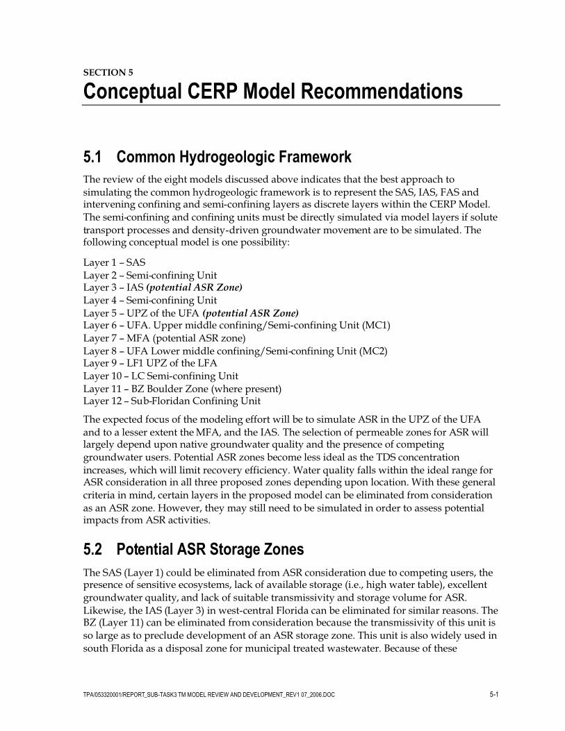
5.1 Common Hydrogeologic Framework
The review of the eight models discussed above indicates that the best approach to
simulating the common hydrogeologic framework is to represent the SAS, IAS, FAS andintervening confining and semi-confining layers as discrete layers within the CERP Model.
The semi-confining and confining units must be directly simulated via model layers if solute
transport processes and density-driven groundwater movement are to be simulated. Thefollowing conceptual model is one possibility:
Layer 1 – SAS
Layer 2 – Semi-confining UnitLayer 3 – IAS (potential ASR Zone)
Layer 4 – Semi-confining Unit
Layer 5 – UPZ of the UFA (potential ASR Zone)Layer 6 – UFA. Upper middle confining/Semi-confining Unit (MC1)
Layer 7 – MFA (potential ASR zone)
Layer 8 – UFA Lower middle confining/Semi-confining Unit (MC2)Layer 9 – LF1 UPZ of the LFA
Layer 10 – LC Semi-confining Unit
Layer 11 – BZ Boulder Zone (where present)Layer 12 – Sub-Floridan Confining Unit
The expected focus of the modeling effort will be to simulate ASR in the UPZ of the UFA
and to a lesser extent theMFA, and the IAS. The selection of permeable zones for ASR willlargely depend upon native groundwater quality and the presence of competing
groundwater users. Potential ASR zones become less ideal as the TDS concentration
increases, which will limit recovery efficiency. Water quality falls within the ideal range forASR consideration in all three proposed zones depending upon location. With these general
criteria in mind, certain layers in the proposed model can be eliminated from consideration
as an ASR zone. However, they may still need to be simulated in order to assess potentialimpacts from ASR activities.
5.2 Potential ASR Storage Zones
The SAS (Layer 1) could be eliminated from ASR consideration due to competing users, thepresence of sensitive ecosystems, lack of available storage (i.e., high water table), excellent
groundwater quality, and lack of suitable transmissivity and storage volume for ASR.
Likewise, the IAS (Layer 3) in west-central Florida can be eliminated for similar reasons. TheBZ (Layer 11) can be eliminated from consideration because the transmissivity of this unit is
so large as to preclude development of an ASR storage zone. This unit is also widely used in
south Florida as a disposal zone for municipal treated wastewater. Because of these

TPA/053320001/REPORT_SUB-TASK3 TM MODEL REVIEW AND DEVELOPMENT_REV1 07_2006.DOC 5-2
considerations, the SAS, IAS (in west-central Florida), and BZ can be ruled out as potential
ASR storage zones.
The UPZ of the UFA is widely used as an ASR storage zone in Florida. It generally coincides
with the Tampa member of the Arcadia Formation and the Suwannee Limestone. There are
no active ASR systems in Florida that utilize deeper aquifers than the UPZ for ASR storage.There is at least one system in the planning stages that will use LPZ of the UFA or the the
associatedMFA for an ASR storage zone. This permeable zone is generally found within the
upper portion of the Avon Park Formation. These two zones would be the primary targetsfor developing the CERP network of ASR wells. Locally in southwest Florida, the Lower
Hawthorn Producing Zone (IAS) is currently utilized as a source of groundwater for reverse
osmosis water treatment in Lee County and could be utilized as an ASR storage zone. Thereare few competing users of this zone due to the availability of good quality water in
shallower aquifers.
The LF1 of the LFA is a potential ASR candidate, but is less favorable for development on aregional scale. Due to formation depth and saline water quality, use of LF1 in central Florida
would be precluded because it is a source of good quality water for the Orlando area.
However, after further investigation, these formations may be found to be locally favorablefor ASR development. Elsewhere, the ambient water quality (typically elevated salinity
concentrations) in the LF1 would preclude ASR development. In terms of further
investigation, the permeable zones within the UFA should be considered the best candidatesfor ASR development, followed to a lesser degree by the MFA, and in southwest Florida, the
IAS. The IAS and the MFAhave fewer competing users but have more saline groundwater
quality, whereas the UPZ of the UFA has better quality groundwater but a greater numberof competing users. These factors (competing users and ambient groundwater quality) are
among several that must be carefully evaluated to determine utility for ASR development.
5.3 Discussion of Model Framework
5.3.1 SAS
The SAS is present throughout the area simulated by the fivemodels. Horizontal hydraulic
conductivity and thickness are reasonably well known. Vertical hydraulic conductivity is
less well known but can be extrapolated in most cases from measured values of horizontalhydraulic conductivity. Through most of peninsular Florida, the SAS consists of
unconsolidated deposits of sand, shell, and clay. In south Florida, there is a significant
limestone component to the SAS. It is known locally as the Lower Tamiami Aquifer (LTA).In this area, the SAS is composed of an upper unconfined aquifer, which overlies the
confined LTA. In southeast Florida, the Biscayne aquifer has a significant limestone
component.
5.3.2 Confining and Semi-confining Units
Direct simulation of the confining and semi-confining units will be problematic because
little data is available that characterizes their hydraulic properties. In most cases, only
leakance is available when vertical hydraulic conductivity and thickness are needed.

TPA/053320001/REPORT_SUB-TASK3 TM MODEL REVIEW AND DEVELOPMENT_REV1 07_2006.DOC 5-3
Hydraulic characteristics of the confining unit below the SAS are fairly well known. This
unit retards the flow of groundwater between the SAS and the underlying IAS (wherepresent). Where the IAS is not present, the confining unit is designated as the ICU. The ICU
separates the SAS from the underlying UFA. In areas where the IAS or ICU is not present,
the UFA is considered unconfined. In areas where the ICU is present, the hydraulicproperties of model Layers 2 through 4 must be modified so that they collectively simulate a
confining unit, the ICU. In areas where both the ICU and IAS are not present and the UFA is
unconfined, Layers 1 through 4 would be rendered inactive. Reese (2004) identified threeconfining units (MC1, MC2, and LC) in the FAS. MC1 is equivalent to middle confining unit
I or II of Miller and separates the UFA from theMFA. MC2 is equivalent to middle
confining unit VI of Miller (1986) and separates the MFA from the LFA. LC is found on topof the BZ and is equivalent to middle confining unit VIII (Miller, 1986). The vertical
hydraulic conductivity and thickness values of MC1, MC2, and LC are poorly known and
will be problematic to define in the CERP Model.
5.3.3 Intermediate Aquifer System
The IAS contains significant permeable zones in west-central Florida and southwest Florida.
Three permeable zones, known locally as PZ1, PZ2, and PZ3, have been defined in west-
central Florida south of State Road 60 in Hillsborough County. PZ2 and PZ3 are morewidespread than PZ1 and are found in Sarasota, Desoto, and Charlotte Counties. In
southwest Florida (Lee and Collier Counties) the IAS contains the Sandstone Aquifer and
the Mid-Hawthorn Aquifer. Both aquifers are significant sources of potable water supply inthese counties. Outside of southwest Florida and west-central Florida, the IAS is not present
and consists instead of significant confining units known as the ICU. CH2MHILL
recommends that the IAS be simulated as one active layer in west-central Florida and as twoactive layers in southwest Florida. Outside of these two areas, the IAS layers should be
simulated as semi-confining units representing the ICU. The hydraulic characteristics of the
IAS and ICU are fairly well known.
5.3.4 Upper Floridan Aquifer
The UFA can be simulated as one discrete permeable unit, which is the approach of the SD
Model, Peninsular Model, ETB Model, and DWRM. The LEC Model and EC Model
simulated the UFA as two or more active model layers. Two dominant permeable zones
were established in the UFAwithin the wider model area. Hydraulic characteristics of theUPZ and LPZ of the UFA are fairly well defined and different in magnitude, with the LPZ
being considerable more transmissive. There is ample evidence from APTs in Florida thatthe two permeable units act as one hydraulic unit with little confinement between them. As
a result, the common approach has been to simulate the UFA as one model layer and utilize
hydraulic properties as an average of the two units. However, hydraulic properties for bothpermeable zones are sufficiently well known to warrant delineation as two separate layers.
The UPZ of the UFA is commonly found in the Suwannee Limestone and lower Miocene
formations, whereas the LPZ is commonly found at the bottom of the Ocala Limestone, or
top of the Avon Park Formation. In central and eastern Florida, the Suwannee Limestone isnot present and the UPZ is found at the top of the Ocala Limestone. Based upon the review
of all eight models, CH2M HILL recommends that the UFA be simulated with two active
TPA/053320001/REPORT_SUB-TASK3 TM MODEL REVIEW AND DEVELOPMENT_REV1 07_2006.DOC 5-4
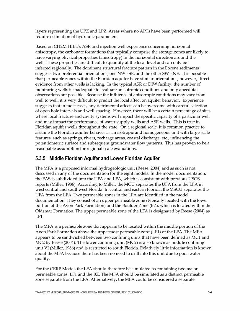
layers representing the UPZ and LPZ. Areas where no APTs have been performed will
require estimation of hydraulic parameters.
Based on CH2MHILL’s ASR and injection well experience concerning horizontal
anisotropy, the carbonate formations that typically comprise the storage zones are likely to
have varying physical properties (anisotropy) in the horizontal direction around thewell. These properties are difficult to quantify at the local level and can only be
inferred regionally. The dominant structural fracture pattern in the Eocene sediments
suggests two preferential orientations, one NW - SE, and the other SW - NE. It is possiblethat permeable zones within the Floridan aquifer have similar orientations, however, direct
evidence from other wells is lacking. In the typical ASR or DIW facility, the number of
monitoring wells is inadequate to evaluate anisotropic conditions and only anecdotalobservations are possible. Because the influence of anisotropic conditions may vary from
well to well, it is very difficult to predict the local affect on aquifer behavior. Experience
suggests that in most cases, any detrimental affects can be overcome with careful selectionof open hole intervals and well spacing. However, there will be a certain percentage of sites
where local fracture and cavity systemswill impact the specific capacity of a particular well
and may impact the performance of water supply wells and ASR wells. This is true inFloridan aquifer wells throughout the state. On a regional scale, it is common practice to
assume the Floridan aquifer behaves as an isotropic and homogeneous unit with large scale
features, such as springs, rivers, recharge areas, coastal discharge, etc., influencing thepotentiometric surface and subsequent groundwater flow patterns. This has proven to be a
reasonable assumption for regional scale evaluations.
5.3.5 Middle Floridan Aquifer and Lower Floridan Aquifer
The MFA is a proposed informal hydrogeologic unit (Reese, 2004) and as such is notdiscussed in any of the documentation for the eight models. In the model documentation,
the FAS is subdivided into the UFA and LFA, which is consistent with previous USGS
reports (Miller, 1986). According to Miller, theMCU separates the UFA from the LFA inwest central and southwest Florida. In central and eastern Florida, theMSCU separates the
UFA from the LFA. Two permeable zones in the LFA are identified in the model
documentation. They consist of an upper permeable zone (typically located with the lowerportion of the Avon Park Formation) and the Boulder Zone (BZ), which is located within the
Oldsmar Formation. The upper permeable zone of the LFA is designated by Reese (2004) as
LF1.
The MFA is a permeable zone that appears to be located within the middle portion of the
Avon Park Formation above the uppermost permeable zone (LF1) of the LFA. The MFA
appears to be sandwiched between two confining units that have been defined as MC1 andMC2 by Reese (2004). The lower confining unit (MC2) is also known as middle confining
unit VI (Miller, 1986) and is restricted to south Florida. Relatively little information is known
about theMFA because there has been no need to drill into this unit due to poor waterquality.
For the CERP Model, the LFA should therefore be simulated as containing two major
permeable zones: LF1 and the BZ. The MFA should be simulated as a distinct permeablezone separate from the LFA. Alternatively, theMFA could be considered a separate

TPA/053320001/REPORT_SUB-TASK3 TM MODEL REVIEW AND DEVELOPMENT_REV1 07_2006.DOC 5-5
permeable zone of the LFA. However, because there are significant confining units
separating the MFA from the UFA above and LFA below, it was decided to define it as aseparate aquifer. Relatively little hydraulic data is available for theMFA and LFA due to
availability of good quality water in shallower aquifers. Groundwater quality in the LFA
(LF1) is relatively poor in west-central, southwest, and south Florida. In central and easternFlorida, groundwater quality is relatively good in LF1, which in these areas of Florida is
utilized extensively as a source of drinking water. The lowermost permeable zone of the
LFA is the BZ and is typically found within the Oldsmar Formation.
5.4 Discussion of Model Grid or Mesh Spacings
The USACE intends to use a finite- element approach to the model simulations. It is difficult
to determine the number of elements that will be required without knowing the exactgeometry of the elements in the proposed finite-element model. Each finite-element model
is different and different element configurations can be used (i.e., trapezoid verses
triangular).All of the models reviewed utilized the finite-difference mathematicalformulation. Most of the models used 2,500-foot to 5,000-foot uniform cell sizes depending
on the size of the model study area and the detail the authors were targeting without
exceeding the available computing power.
Assuming the model will cover an area from north of Orlando to the Florida Keys and from
the east coast to the west coast, the dimensions of the model will be approximately 150 miles
from east to west and 300 miles from north to south. Given our level of understanding of thedistribution of aquifer properties in peninsular Florida it would be appropriate to assume
that cell size or element size should approximate one mile or a significant portion of one
mile in dimension. Of course, the greater the resolution required, the greater the processingpower required. A compromise must be reached that accounts for the desired resolution of
the mathematical model and the availability of processing power and speed. A rough
estimate of the number of finite-difference cells required for the model assuming certain cellsizes and 12 model layers is provided below:
Cell Size No. Columns No. Rows No. of Cells or Calculation Points
1 Mile 150 300 45,000
0.5 Mile 300 600 180,000
0.25 Mile 600 1,200 720,000
Square shaped cells are assumed, that is cell dimensions are the same along the X and Y
axis. An aspect ratio of up to 5 can be used in most finite-element models so the geometry ofthe cells/elements can easily deviate from the square. The number of cells or calculation
points would increase accordingly if the number of layers used to simulate the
hydrogeologic regime is increased. As many of 24 layers (2 model layers per hydrogeologiclayer) may be utilized to achieve the desired level of accuracy.

TPA/053320001/REPORT_SUB-TASK3 TM MODEL REVIEW AND DEVELOPMENT_REV1 07_2006.DOC 6-1
SECTION 6
Recommended CERP Model Framework
Twelve layers are recommended for the CERP Model to simulate the hydrologic regime of
peninsular Florida. This layering scheme (previously presented) includes seven semi-
confining/confining units and seven permeable units. The permeable units consist of theSAS (Layer 1), IAS (Layer 3), UPZ of the UFA (Layer 5), MFA (Layer 7), LF1 (Layer 9), and
BZ (Layer 11).
Alternatively, the model framework can be reduced to 10 layers if the IAS is not simulatedbecause it is only present in west-central Florida and southwest Florida. The SAS and BZ
could also be simulated as arrays of constant heads to further simplify the CERP Model.

TPA/053320001/REPORT_SUB-TASK3 TM MODEL REVIEW AND DEVELOPMENT_REV1 07_2006.DOC 7-1
SECTION 7
References
Bower, et al. 1990. A Three-Dimensional Finite Difference GroundWater Model of Lee
County, Florida. Technical Publication 90-01. South Florida WaterManagement District.
West Palm Beach, Florida.
Fairbank, P., J. Valdes, E. Rectenwald, M. Switaneck, and E. Hopkins. 1999. Documentation
for the Lower East Coast Floridan Aquifer Model. South Florida Water Management
District.West Palm Beach, Florida.
Florida Geological Survey. 2003. Update of the Hydrogeology of SWFWMD. (FGS, in
preparation).
Lukasciewicz, John. 1992.A Three-dimensional Finite Difference Groundwater Flow Model of theFloridan Aquifer System in Martin, St. Lucie and eastern Okeechobee Counties, Florida. SFWMD
Technical Publication 92-03.
McGurk, B., and P. Fischl Presley. 2002. Simulation of the Effects of GroundwaterWithdrawals on the Floridan Aquifer System in East-Central Florida: Model Expansion and
Revision. Technical Publication SJ2002-3. St. Johns River Water Management District.
Palatka, FL.
Miller, J.A. 1986. Hydrogeologic Framework of the Floridan Aquifer System in Florida and Parts of
Georgia, Alabama and South Carolina. Professional Paper 1403-B. Washington, D.C.: U.S.
Geological Survey.
O’Reilly, A.M., R.M. Spechler, and B.E. McGurk. 2002.Hydrogeology and Water-Quality
Characteristics of the Lower Floridan Aquifer in East-Central Florida. U.S. Geological Survey
WRIR 02-4193.
Randazzo, A. F., and D. S. Jones. 1997. The Geology of Florida, University Press of Florida.
Reese, R.S. & R.J. Memberg. 1999.Hydrogeology and the Distribution of Salinity in the Floridan
Aquifer System, Palm Beach County, Florida.U.S. Geological Survey. WRIR 99-4061.
Reese, R.S. 1994. Hydrogeology and the Distribution and Origin of Salinity in the Floridan Aquifer
System, Southeastern, Florida.WRIR 94-4010. U.S. Geological Survey.
Reese, R.S. 2000. Hydrogeology and the Distribution of Salinity in the Floridan Aquifer System,Southwestern, Florida.U.S. Geological Survey. WRIR 98-4253.
Reese, R.S. 2003. Hydrogeology, Water Quality, and the Distribution and Sources of Salinity in the
Floridan Aquifer System, Martin and St. Lucie Counties, Florida. U.S. Geological Survey. WRIR03-4242.
Reese, R.S. 2004. Preliminary Hydrogeologic Framework.

Tables
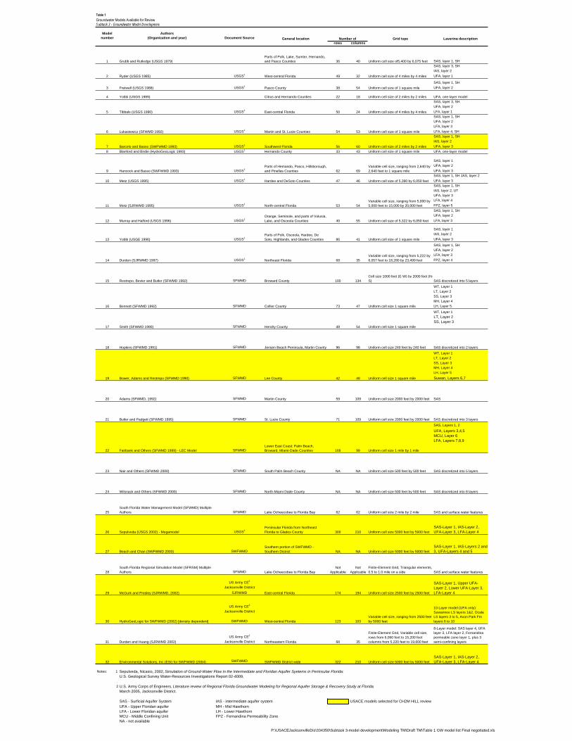
Model Authors
number (Organization and year) Document Source
rows columns
SAS, layer 1, SH
SAS, layer 3, SH
IAS, layer 2
USGS1
UFA, layer 1
SAS, layer 1, SH
USGS1
UFA, layer 2
4 Yobbi (USGS 1989) Citrus and Hernando Counties 22 18 Uniform cell size of 2 miles by 2 miles UFA, one-layer model
SAS, layer 3, SH
UFA, layer 2
USGS1
LFA, layer 1
SAS, layer 1, SH
UFA, layer 2
LFA, layer 3
USGS1
LFA, layer 4, SH
SAS, layer 1, SH
IAS, layer 2
USGS1
UFA, layer 3
8 Blanford and Birdie (HydroGeoLogic 1993) USGS1
Hernando County 33 43 Uniform cell size of 1 square mile UFA, one-layer model
SAS, layer 1
UFA, layer 2
USGS1
UFA, layer 3
SAS, layer 1, SH JAS, layer 2
USGS1
UFA, layer 3
SAS, layer 1, SH
IAS, layer 2, UT
UFA, layer 3
LFA, layer 4
USGS1
FPZ, layer 5
SAS, layer 1, SH
UFA, layer 2
USGS1
LFA, layer 3
SAS, layer 1
IAS, layer 2
USGS1
UFA, layer 3
SAS, layer 1, SH
UFA, layer 2
LFA, layer 3
USGS1
FPZ, layer 4
SFWMD
WT, Layer 1
LT, Layer 2
SS, Layer 3
MH, Layer 4
SFWMD LH, Layer 5
WT, Layer 1
LT, Layer 2
SS, Layer 3
SFWMD
SFWMD
WT, Layer 1
LT, Layer 2
SS, Layer 3
MH, Layer 4
LH, Layer 5
SFWMD Suwan, Layers 6,7
SFWMD
SFWMD
SAS, Layers 1, 2
UFA, Layers 3,4,5
MCU, Layer 6
LFA, Layers 7,8,9
SFWMD
SFWMD
SFWMD
SFWMD
USGS1
SWFWMD
SFWMD
US Army CE2
Jacksonville District
SJRWMD
US Army CE2
Jacksonville District
SWFWMD
US Army CE2
Jacksonville District
SWFWMD
Notes: 1 Sepulveda, Nicasio, 2002, Simulation of Ground-Water Flow in the Intermediate and Floridan Aquifer Syetems in Peninsular Florida:
U.S. Geological Survey Water-Resources Investigations Report 02-4009,
2 U.S. Army Corps of Engineers, Literature review of Regional Florida Groundwater Modeling for Regional Aquifer Storage & Recovery Study at Florida.
March 2005, Jacksonville District.
SAS - Surficial Aquifer System IAS - intermediate aquifer system USACE models selected for CH2M HILL review
UFA - Upper Floridan aquifer MH - Mid Hawthorn
LFA - Lower Floridan aquifer LH - Lower Hawthorn
MCU - Middle Confining Unit FPZ - Fernandina Permeability Zone
NA - not available
210 Uniform cell size 5000 feet by 5000 feet
SAS-Layer 1, IAS-Layer 2,
UFA-Layer 3, LFA-Layer 4 32 Environmental Solutions, Inc (ESI) for SWFWMD (2004) SWFWMD District wide 322
35
Finite-Element Grid, Variable cell size,
rows from 6,060 feet to 15,200 feet
columns from 5,220 feet to 19,600 feet
8-Layer model: SAS layer 4, UFA
layer 3, LFA layer 2, Fernandina
permeable zone layer 1, plus 3
semi-confining layers31 Durden and Huang (SJRWMD 2002) Northeastern Florida 68
194 Uniform cell size 2500 feet by 2500 feet
SAS-Layer 1, Upper UFA-
Layer 2, Lower UFA-Layer 3,
LFA-Layer 4
30 HydroGeoLogic for SWFWMD (2002) [density dependent] West-central Florida 123 103
Variable cell size, ranging from 2500 feet
by 5000 feet
10-Layer model (UFA only):
Suwannee LS layers 1&2, Ocala
LS layers 3 to 5, Avon Park Fm
layers 6 to 10
29 McGurk and Presley (SJRWMD, 2002) East-central Florida 174
Uniform cell size 5000 feet by 5000 feet
SAS-Layer 1, IAS-Layer 2,
UFA-Layer 3, LFA-Layer 4 Sepulveda (USGS 2002) - Megamodel26
Peninsular Florida from Northeast
Florida to Glades County 300 210
62
South Florida Water Management Model (SFWMD) Multiple
Authors Lake Ocheecobee to Florida Bay 62 Uniform cell size 2 mile by 2 mile SAS and surface water features
28
South Florida Regional Simulation Model (SFRSM) Multiple
Authors Lake Ocheecobee to Florida Bay
Not
Applicable
Not
Applicable
Finite-Element Grid, Triangular elements,
0.5 to 1.0 mile on a side SAS and surface water features
25
SAS discretized into 5 layers
24 Wilsnack and Others (SFWMD 2000) North-Miami Dade County NA NA Uniform cell size 500 feet by 500 feet SAS discretized into 8 layers
NA Uniform cell size 500 feet by 500 feet
22 Fairbank and Others (SFWMD 1999) - LEC Model
23 Nair and Others (SFWMD 2000) South Palm Beach County NA
Lower East Coast: Palm Beach,
Broward, Miami-Dade Counties 166 99 Uniform cell size 1 mile by 1 mile
SAS
21 Butler and Padgett (SFWMD 1995) St. Lucie County 71 109 Uniform cell size 2000 feet by 2000 feet SAS discretized into 3 layers
20 Adams (SFWMD, 1992)
98 Uniform cell size 240 feet by 240 feet96
109 Uniform cell size 2000 feet by 2000 feetMartin County 59
SAS discretized into 2 layers
19 Bower, Adams and Restrepo (SFWMD 1990) Lee County 42 48 Uniform cell size 1 square mile
18 Hopkins (SFWMD 1991) Jensen Beach Peninsula, Martin County
73 47 Uniform cell size 1 square mile
17 Smith (SFWMD 1990) Hendry County 48 54 Uniform cell size 1 square mile
Table 1
Subtask 3 - Groundwater Model Development
General location Number of Grid type Layering description
Groundwater Models Available for Review
1 Grubb and Rutledge (USGS 1979)
Parts of Polk, Lake, Sumter, Hernando,
and Pasco Counties 36
54 Uniform cell size of 1 square mile
2 Ryder (USGS 1985) West-central Florida 49
40 Uniform cell size of5,400 by 6,075 feet
32 Uniform cell size of 4 miles by 4 miles
24 Uniform cell size of 4 miles by 4 miles
3 Fretwell (USGS 1988)
5 Tibbals (USGS 1990) East-central Florida 50
Pasco County 38
6 Lukasiewicz (SFWMD 1992) Martin and St. Lucie Counties 54
69
Variable cell size, ranging from 2,640 by
2,640 feet to 1 square mile
7 Barcelo and Basso (SWFWMD 1993) Southwest Florida 56
53 Uniform cell size of 1 square mile
60 Uniform cell size of 2 miles by 2 miles
46 Uniform cell size of 5,390 by 6,050 feet
9 Hancock and Basso (SWFWMD 1993)
10 Metz (USGS 1995) Hardee and DeSoto Counties 47
Parts of Hemando, Pasco, Hillsborough,
and Pinellas Counties 62
11 Motz (SJRWMD 1995) North-central Florida 53
41 Uniform cell size of 1 square mile
12 Murray and Halford (USGS 1996)
Orange, Seminole, and parts of Volusia,
Lake, and Osceola Counties 40
54
Variable cell size, ranging from 5,000 by
5,000 feet to 15,000 by 20,000 feet
55 Uniform cell size of 5,322 by 6,050 feet
35
Variable cell size, ranging from 5,222 by
6,057 feet to 18,280 by 23,499 feet
13 Yobbi (USGE 1996)
14 Durden (SJRWMD 1997) Northeast Florida 68
Parts of Polk, Osceola, Hardee, De
Soto, Highlands, and Glades Counties 86
SAS discretized into 5 layers134
Cell size 1000 feet (E-W) by 2000 feet (N-
S)
16 Bennett (SFWMD 1992) Collier County
15 Restrepo, Bevier and Butler (SFWMD 1992) Broward County 100
NA Uniform cell size 5000 feet by 5000 feet
SAS-Layer 1, IAS-Layers 2 and
3, UFA-Layers 4 and 5 27 Beach and Chan (SWFWMD 2003)
Southern portion of SWFWMD -
Southern District NA
P:\USACEJacksonvilleDis\334350\Subtask 3-model development\Modeling TM\Draft TM\Table 1 GW model list Final negotiated.xls
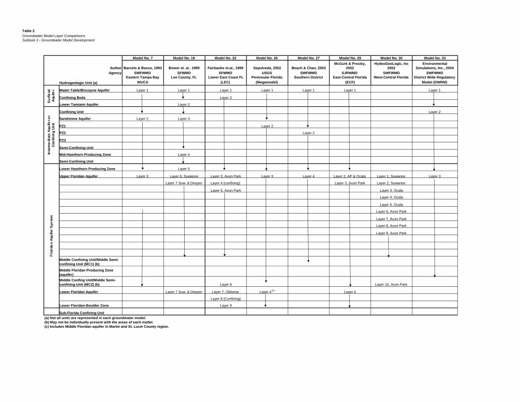
Table 2
Groundwater Model Layer Comparisons
Subtask 3 - Groundwater Model Development
Model No. 7 Model No. 19 Model No. 22 Model No. 26 Model No. 27 Model No. 29 Model No. 30 Model No. 33
Author Barcelo & Basso, 1993 Bower et. al.. 1990 Fairbanks et.al., 1999 Sepulveda, 2002 Beach & Chan, 2003
McGurk & Presley,
2002
HydeoGeoLogic, Inc
2002
Environmental
Simulations, Inc., 2004
Agency SWFWMD SFWMD SFWMD USGS SWFWMD SJRWMD SWFWMD SWFWMD
Hydrogeologic Unit (a)
Eastern Tampa Bay
WUCA
Lee County, FL Lower East Coast FL
(LEC)
Peninsular Florida
(Megamodel)
Southern District East-Central Florida
(ECF)
West-Central Florida District Wide Regulatory
Model (DWRM)
Water-Table/Biscayne Aquifer Layer 1 Layer 1 Layer 1 Layer 1 Layer 1 Layer 1 Layer 1
Confining Beds Layer 2
Lower Tamiami Aquifer Layer 2
Confining Unit Layer 2
Sandstone Aquifer Layer 2 Layer 3
PZ1 Layer 2
PZ2 Layer 2
PZ3
Semi-Confining Unit
Mid-Hawthorn Producing Zone Layer 4
Semi-Confining Unit
Lower Hawthorn Producing Zone Layer 5
Upper Floridan Aquifer Layer 3 Layer 6, Suwanee Layer 3, Avon Park Layer 3 Layer 4 Layer 2, AP & Ocala Layer 1, Suwanee Layer 3
Layer 7 Suw. & Deeper Layer 4 (confining) Layer 3, Avon Park Layer 2, Suwanee
Layer 5, Avon Park Layer 3, Ocala
Layer 4, Ocala
Layer 5, Ocala
Layer 6, Avon Park
Layer 7, Avon Park
Layer 8, Avon Park
Layer 9, Avon Park
Middle Confining Unit/Middle Semi-
confining Unit (MC1) (b)
Middle Floridan Producing Zone
(aquifer)
Middle Confing Unit/Middle Semi-
confining Unit (MC2) (b) Layer 6 Layer 10, Avon Park
Lower Floridan Aquifer Layer 7 Suw. & Deeper Layer 7, Oldsmar Layer 4(c)
Layer 4
Layer 8 (Confining)
Lower Floridan-Boulder Zone Layer 9
Sub-Florida Confining Unit
(a) Not all units are represented in each groundwater model.
(b) May not be individually present with the areas of each model.
(c) Includes Middle Floridan aquifer in Martin and St. Lucie County region.
Su
rfic
ial
Aqu
ife
r
Inte
rme
dia
teA
qu
ife
ro
r
Con
fin
ing
Un
itF
lori
da
nA
qu
ifer
Sys
tem

Figures
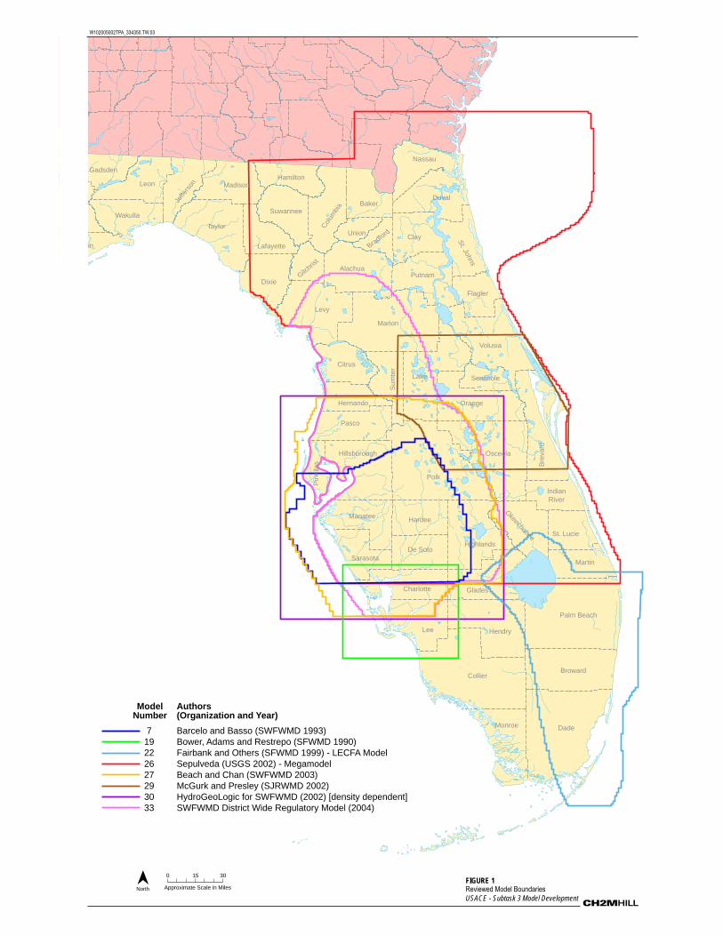
Franklin
Gadsden
Leon
Wakulla
Alachua
Baker
Bradfo
rd
Bre
vard
Broward
Charlotte
Citrus
Clay
Collier
Col
umbi
a
Dade
De Soto
Dixie
Duval
Flagler
Gilc
hrist
Glades
Hamilton
Hardee
Hendry
Hernando
Highlands
Hillsborough
Indian
River
Jeffe
rson
Lafayette
Lake
Lee
Levy
Madison
Manatee
Marion
Martin
Monroe
Okeechobee
Palm Beach
Pasco
Pin
ella
s
Polk
Putnam
St. Jo
hns
St. Lucie
Sarasota
Seminole
Sum
ter
Suwannee
TaylorUnion
Volusia
Liberty
Orange
Osceola
Nassau
W102005002TPA_334350.TW.03
North
FIGURE 1
Reviewed Model Boundaries
USACE - Subtask 3 Model Development
7
19
22
26
27
29
30
33
Barcelo and Basso (SWFWMD 1993)
Bower, Adams and Restrepo (SFWMD 1990)
Fairbank and Others (SFWMD 1999) - LECFA Model
Sepulveda (USGS 2002) - Megamodel
Beach and Chan (SWFWMD 2003)
McGurk and Presley (SJRWMD 2002)
HydroGeoLogic for SWFWMD (2002) [density dependent]
SWFWMD District Wide Regulatory Model (2004)
ModelNumber
Authors(Organization and Year)
0 3015
Approximate Scale in Miles
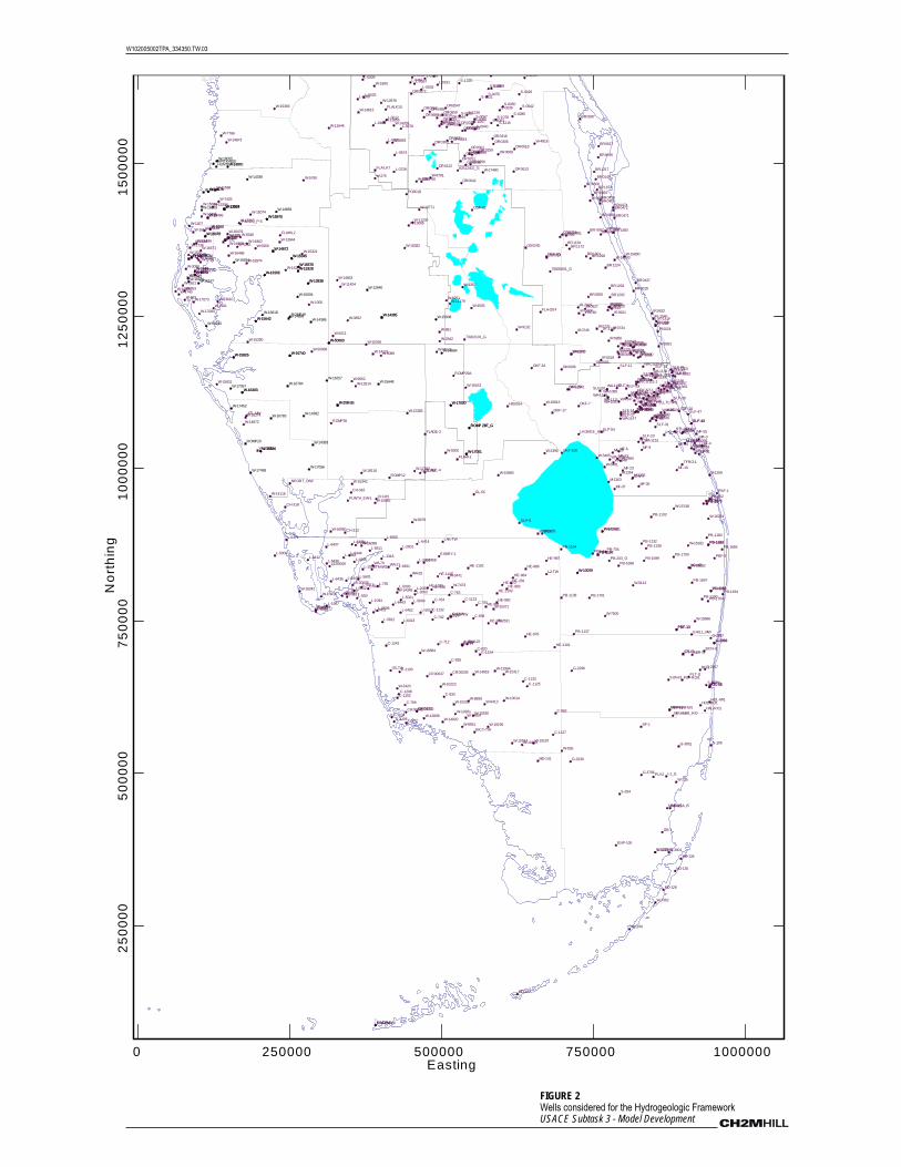
0 250000 500000 750000 1000000Easting
25
00
00
50
00
00
75
00
00
No
rth
ing
15
00
00
01
00
00
00
12
50
00
0
W-15382
W-13065
W-2420
W-8899
W-8951
W-9413W-10014
W-10180
W-10183W-10184 W-10187
W-10190
W-10201
W-10202
W-10223
W-12838
W-14919
W-14920
W-11179
W-11424
W-14934
W-15122
W-15317
MDWSA_I5
LKOKEE_ASR
MF-37
I-1_G
MF-4
MF-6MF-20
SLF-6
SLF-16
SLF-54
W-3852
W-4503
W-9211
W-9251
W-12296
OKF-29
W-215
W-935
W-7473
W-15371
W-13850
W-14703
W-16039
SL00033
MT00045MT00053
OK0003
OK0005
OK0006
IR0498
IR0623IR0638
IR0640
IR0696
IR0706
LE00005
LE00009
IR0024
IR0319
IR0323IR0325IR0329IR0330
HI00014
W-15880
W-2396
W-2912W-5435
W-16543
W-16897
W-16884
W-50003
W-9132
W-14385
W-14663
BF-1
SLF-11
SLF-14
SLF-26
MF-3
MF-31
MF-35
SLF-50
SLF-9SLF-21
SLF-46
SLF-47
WA-1001
WA-1107
WA-1111
WA-1144
WA-1147
WA-546
WA-547
WA-562
OSF-85
OKF-34
MF-33
PBF-3
WA-565WA-580WA-582
WA-1009 WA-1032
WA-699
SLF-4
SLF-23
SLF-40
PBF-1
SLF-20
SLF-31
SLF-42
SLF-43SLF-44
MF-34
MF-36B
SLF-53
PB-203_G
WA-70
G-2296
MF-1
W-4818
W-5881W-8781
W-17480
D-365
MIRAMARIW1
W-14348W-15916
W-16098
W-16242
W-16960
W-18091
W-5405
W-6173
W-12542
W-15813
W-2860
W-5441
W-1976
W-7362
W-01511
W-9300
W-15163
W-17000
W-17001
W-1022
W-4086
W-17392W-18116
W-275
W-1893
W-909
W-13881
W-15890W-16133
75805501_G
L2-TW
SLF-17
MF-23
OKF-7
OKF-17
SLF-45
DF-1
G-3706
L-5812
S-1533_G
82512401_G
G-2916
G-2917C-1103
C-1106
C-1125
C-1127
W-7500
W-9112
W-10079W-10080
W-15748
W-15886
W-16052
W-16182
W-16234
W-16882
W-17052
PB-1764
PB-1194
PB-1137
PB-1170
PB-1693
W-9062
W-9089
W-13514
W-14121
W-15346
W-8079
W-15343
PB-1138
PB-1186
W-2631
W-3441
PB-747
S-156
MF-9
PB-1689
SLF-28
L-5003L-5013
L-5009
L-6461
L-2061
L-6435
L-6437
L-6471
L-2458
PBP-I1
CS-I1
C-764
C-712
C-759
W-12994
C-820
L-2460L-4846
L-1044
WA-25
WA-1087WA-1003WA-1006
WA-1016WA-1083
WA-1085
WA-1136
WA-1139
WA-820
WA-823
WA-875WA-878
WA-877WA-887WA-708
SUN-I3PLT-I1
BCN-I1
G-2887
C-739C-1122
HE-281
HE-1105
MF-10
73912101_G
IR-1001
M-1332
M-1352M-1353
M-1357M-1358
M-1359
M-1363
M-1364
M-1366
STL-386
STL-422
WA-1119
WA-1140
WA-1151
WA-1155
WA-1158
WA-1186
WA-1192
C-727
C-753
C-932
C-933
C-935
C-938
C-962
C-1123
C-1132
C-1133
G-3239
HE-976
HE-981HE-982
HE-983
HE-984
HE-986
HE-987
BR-0910
L-0729
S-1215WREG170S-1078
S-1225
PB-1187
PB-1190
PB-1193
PB-1197
PB-1690
PB-1697
PB-1698
PB-1699PB-1700
PB-1701
CH-318
C-1102
L-2901
C-719C-851
HE-948
HE-973
W-16274
W-17505W-15636
W-14116
NPORT_DIW
W-16574
W-2607
W-16740
PASCO_P-5
W-15321
W-15345
W-16576
W-17073
W-15826
L-6463
MF-55
NRCS2-1NRCS7-1
NRCS29-8
NRCS121-1
G-2889HE-1101
MAR-I2CS-I2
PB-652
PB-734
PB-1132
PB-1133
PB-1139
SLF-0049
SLF-48
PB-1164
PB-1171
PB-1180
GLF-6
CH-313
I75-TW
OKF-100
G-3061
MIRAMAR_RO
LAB-TW
PBF-7
PAHO-MZL
GL-5C
AID-MZL
PBF-13
ROMP-25
BICY-TW
IWSD-TW
WA-21
CH-R5
CR00037 CR00039
OR0072
OR0122OR0249OR0250
OR0251
OR0254OR0255OR0259
OR0301
OR0303 OR0305
OR0316
OR0319OR0325OR0329 OR0331
OR0333
OR0341
OR0343
OR0495OR0547
OR0552
OR0610
OR0613
OR0618
OR0620
OR0642
OR0644
OR0659
OS0014
OS0062OS0216
PO0018
ENP-100
C-1124
C-742
C-781
HE-1106HE-970
L-6401 L-6462
HE-1102
HE-1103
L-550
L-755
L-1018
L-1094
L-1318
L-1595
L-1817
L-1967
L-2063L-2657
L-5000
L-5001
L-5010
L-5601
L-5602
L-5605
L-5608
L-5609
L-5615
L-6412
L-6413
L-6436
L-6439
L-6443
L-6444
L-6445
MO-141
W-10862
W-12393
W-11766
FLADE-3
FLADE-4
FLAHI-1
MO-122
FTL-M1
GB-1
HAL-RO1
MO-128
MO-130
MO-134
PLT-ROI1
PU-I2
S-254
S-3001
KWDZMW-1
ICW-1
FPU_RO-IW1
FTL-I3
FLAHIL2
FLA-LK7
FLALK10
FLA-OS4
W-15366
W-7766
W-14873
W-129W-130W-131W-132W-134
W-1005
W-5069
W-5646
W-6232
W-13838
W-13944
W-14274
W-14672
W-15161
W-15280
W-15328
W-15642
W-16462
W-16468
W-16469
W-16479
W-1809
W-12878
W-13855W-14269
W-14813
W-15831
W-16303
W-50089
W-35
W-5760
W-7403
W-11588
W-13924
W-14675
W-15074
W-15296W-15684
W-16495W-16496
W-17067
W-583
W-953
W-1407
W-1614
W-1617
W-1618
W-1619
W-1620
W-1621
W-1647
W-1648W-1649
W-1738
W-1739
W-1740
W-1741W-1743
W-1901
W-2942W-2970W-2971
W-3003
W-3090
W-4760
W-13610
W-14896
W-15204W-15939
W-16471
W-16486
W-16489
W-17084
W-50149
W-981
W-2842
W-9257
W-10771
W-11230
W-14872
W-11646
ROMP29A
BR0015
BR0149
BR0437
BR0446
BR0471
BR0472BR0474
BR0475BR0476
BR0485
BR0492
BR0500
BR0530
BR0587
BR0617
BR0854
BR0920
BR1153
BR1164BR1172
BR1202
BR1224
BR1293
BR1296BR1301
BR1480
IR0615IR0627 IR0628IR0630IR0631
IR0632
IR0730
IR0734IR0735
IR0740
IR0745
IR0779
IR0921
IR0954
IR0956
IR0991
L-0002
L-0009
L-0012
L-0026
L-0031
L-0033
L-0090
L-0111
L-0191
L-0464
L-0467
L-0574
L-0582
L-0587
L-0676
L-0704
OR0621
OR0668
OR0688
S-0026
S-0039
S-0040
S-0042S-0050
S-0063S-0065S-0067
S-0068
S-0075
S-0285
S-0889
S-1021
S-1057
S-1196
S-1216
V-0235V-0239
IR-119F
IR-141F
IR-132F
IR-154F
IR-202F
IR-190F
IR-42F
L-5811
PBF-12
PUNTA_EW-1
C-1208
MDS-I12
C-1104
BR1217
SLF-70
CLW-A1
ATL-MW
C-1246
PSLWPT-IW1
HOL-IW1
PSLLTC-IW1
ORF-60
OSF-82
EHILL_MW
FTM-IW1
C-1242
CH-316
OS0245
TFRO-1
ROMP12
ROMP35
EXBRY-1
KWDIW-1
CR00041CR00042
HOL-RO1
S-567
L-6411
L-6414
W-15938
W-12640
W-50003
W-14385
W-14884
W-17000
W-17001
ROMP 28F_GROMP 28F_G
W-15648
W-17608
W-16784
W-16783
ROMP20
W-15636
W-14383
W-17056
W-16740
ARIPEKA820HUNTERS378
W-15345
W-16576
W-16004
W-16618ROMP49
W-15826
W-16257
W-16303W-17057
W-13923W-13924
W-14336
W-14669
W-14674W-14675
W-15972W-15976
W-16609
W-14673
W-18055
W-13838
W-14386
W-14668
W-14672
W-14888
W-15328
W-15494
W-15642
W-14382
W-15204
W-16181W-16197
W-16573
W-17452
W-17488
W-50015
FIGURE 2
Wells considered for the Hydrogeologic FrameworkUSACE Subtask 3 - Model Development
W102005002TPA_334350.TW.03
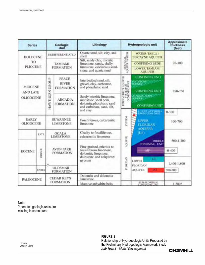
W102005002TPA_334350.TW.03
FIGURE 3
Relationship of Hydrogeologic Units Proposed by the Preliminary Hydrogeologic Framework StudySub-Task 3 - Model Development
Source:Reese, 2004
Note:? denotes geologic units aremissing in some areas

Appendices

APPENDIX A
Southwest Florida Region Model Review TM
TPA/053320002/SOUTHWEST MODEL TM_07_2006_REV1.DOC 1
T E C H N I C A L M E M O R A N D U M
Southwest Florida Region Groundwater ModelReview: Sepulveda (2002), Beach and Chan (2003),Barcelo and Basso (1993), HydroGeoLogic (2002), andEnvironmental Simulations, Inc. (2004)
PREPARED FOR: US Army Corp of Engineers
PREPARED BY: CH2M HILL
DATE: December 14, 2005
PROJECT NUMBER: 334350.TW.03
Contents
Introduction and Purpose ............................................................................................................1
Comparison of Model Frameworks............................................................................................2Model Summaries..........................................................................................................................4
Sepulveda, 2002. Simulation of Groundwater Flow in the Intermediate and
Floridan Aquifer Systems in Peninsular Florida, U.S. Geological SurveyWater-Resources Investigations Report 02-4009. ..........................................................4
Beach and Chan, 2003. Southern District Groundwater Flow ModelVersion 1.0, Prepared by the Hydrologic Evaluation Section, Resource
Conservation and Development Department, Southwest Florida Water
Management.......................................................................................................................8
Barcelo and Basso, 1993. Computer Model of Groundwater Flow in theEastern Tampa Bay Water Use Caution Area: Southwest Florida Water
Management District.......................................................................................................10
HydroGeoLogic, Inc., June 2002. Three-Dimensional Density-DependantFlow and Transport Modeling of Saltwater Intrusion in the
Southern Water Use Caution Area................................................................................13
Environmental Simulations, Inc., April 2004. Development of theDistrict Wide Regulation Model for Southwest Florida Water
Management District.......................................................................................................15
Introduction and Purpose
The goal of this project is to collect and summarize data from available model
documentation and provide recommendations to the U.S. Army Corps of Engineers(USACE) Jacksonville District for the development of a Regional Groundwater Model of
Florida. This Technical Memorandum (TM) summarizes the model reviews for northern and
west-central Florida. A second TM has been prepared that summarizes three separatemodels fromcentral and south Florida.
SOUTHWEST FLORIDA REGION GROUNDWATER MODEL REVIEW: SEPULVEDA (2002), BEACH AND CHAN(2003), BARCELO AND BASSO (1993), HYDROGEOLOGIC(2002), AND ENVIRONMENTAL SIMULATIONS, INC. (2004)
TPA/053320002/SOUTHWEST MODEL TM_07_2006_REV1.DOC 2
Fivemodels were reviewed:
Peninsular Model (Sepulveda, 2002)
Southern District of SWFWMDModel (Beach and Chan, 2003)
Eastern Tampa Bay Model (Barcelo and Basso, 1993)
HydroGeoLogic Model (HydroGeoLogic, 2002)
District Wide Regulatory Model (Environmental Simulations, Inc. [ESI], 2004)
Figure 1 shows the geographic relationship between the five model areas.
Comparison of Model Frameworks
The Peninsular Model developed by Sepulveda (2002) extends from Charlton and CamdenCounties in southGeorgia to near the Palm Beach County –Martin County line in south
Florida. The Beach and ChanModel (2003), known as the Southern District (SD) Model,
encompasses a smaller area, from Hernando County in the north to Lee County in the southand from the Gulf of Mexico in the west to the Kissimmee River in the east. The Eastern
Tampa Bay (ETB) Model (Barcelo and Basso, 1993) is an earlier version of the SDModel and
includes a smaller area, extending fromHillsborough County in the north to Charlotte Countyin the south, from the Gulf of Mexico in the west to Polk County in the east. The SDModel
area includes all of the ETBModel area, while the Peninsular Model includes the areas of both
the ETBModel and the SDModel. The District Wide Regulatory (DWR) Model (ESI, 2004) is asmaller subset of the Peninsular Model and coincides with the boundaries of the Southwest
Florida Water Management District (SWFWMD) plus a buffer zone of approximately 10 miles
on all sides. The southern boundary of the DWRModel was extended past the southernboundary of the Peninsular Model to coincide with the southern boundary of the SWFWMD.
TheHydroGeoLogic Model (2002) is a smaller subset of the SDModel and includes the
southern half of Hillsborough County and all of Manatee and Sarasota Counties. Unlike theother models, theHydroGeoLogic Model simulates solute transport and density-driven
groundwater movement. All five models are finite-difference models.
Three aquifer systems are present within the area simulated by the five groundwatermodels. These aquifer systems are identified as the Surficial aquifer system (SAS), the
Intermediate aquifer system (IAS) and the Floridan aquifer system (FAS). The surficial
aquifer system (SAS) is the uppermost water-bearing hydrogeologic unit. The SAS mostlyconsists of variable amounts of sand, clay, sandy clay, shell beds, silt, and clay. The SAS
extends throughout most of the study area, except where the Upper Floridan aquifer (UFA)
is unconfined. The IAS underlies the SAS and extends throughout most of southwest
Florida. State Road 60 is generally considered the northern boundary of the IAS in westernFlorida. The unit consists mainly of clastic sediments interbedded with carbonate rocks that
generally coincide with the Hawthorn Group. Confining beds that overlie the UFA andunderlie the SAS limit the vertical extent of the IAS in west-central Florida. In the absence of
significant permeable zones, the IAS is defined as the intermediate confining unit (ICU). The
ICU is present outside of west-central Florida, wherever the IAS pinches out. The UFA isconsidered to be unconfined in areas where the ICU or IAS is absent or very thin.
The FAS is a thick sequence of limestone and dolomitic limestone of Oligocene and Eocene
ages with highly variable permeability. The FAS is divided into two aquifers of relativelyhigh permeability, referred to as the UFA and the Lower Floridan aquifer (LFA). These
SOUTHWEST FLORIDA REGION GROUNDWATER MODEL REVIEW: SEPULVEDA (2002), BEACH AND CHAN(2003), BARCELO AND BASSO (1993), HYDROGEOLOGIC(2002), AND ENVIRONMENTAL SIMULATIONS, INC. (2004)
TPA/053320002/SOUTHWEST MODEL TM_07_2006_REV1.DOC 3
aquifers are separated by a less permeable unit called the Middle Confining Unit (MCU) in
west-central Florida and in the northwest part of the study area, and the middle semi-confining unit (MSCU) in east-central Florida. The top of the UFA coincides with the top of
the Tampa Member, Suwannee Limestone or the Ocala Limestone, depending upon
location. The bottom of the UFA is the top of the shallowest, significant, regional confiningunit.
In east-central Florida, the UFA and LFA are separated by the MSCU, a sequence of
somewhat permeable, soft, chalky, limestone that locally contains some gypsum and chertand commonly is partially dolomitized. In west-central Florida and in the northwest part of
the study area, the UFA and LFA are separated by the MCU, which is composed of
gypsiferous dolomite and dolomitic limestone of considerably lower permeability than thatof the MSCU in east-central Florida.
Two discrete permeable zones have been defined in the UFA. Theupper permeable zone
(UPZ) has been identified within sections of the Suwannee Limestone and the TampaMemberof the Arcadia Formation. The lower permeable zone (LPZ) of the UFA has been identified
within the lower part of the Ocala Limestone and the upper part of the Avon Park Limestone.
The Ocala Limestone occurs between the Suwannee Limestone and the Avon Park Limestoneand is thought to function as a semi-confining unit between the UPZ and LPZ.
The Middle Floridan aquifer (MFA) as proposed by Reese (2004) is not specifically addressed
within the five models reviewed. Where present, theMFA may be included in either the UPZor LPZ of the UFA, and stratigraphically may be present within the Middle Eocene Avon Park
Formation.
Two discrete permeable zones have been identified in the LFA in northeast Florida. Theyconsist of aUPZ also known as LF1, and the lower Fernandina permeable zone (FPZ). In
south Florida, two permeable zones have also been identified. The upper producing zone
(LF1) is found within the lower portion of the Avon Park Formation below the MCU, whilethe lower producing zone is found in the Oldsmar Formation. The lower producing zone is
known as the “Boulder Zone” due to drilling characteristics and is known for extremely
high transmissivity. The Middle Floridan Aquifer identified by Reese (2004) is not discussedin any of the model documentation.
The five models compared for this TM are provided in Table 1. The PeninsularModel includes
four layers: the SAS, IAS (ICU), UFA, and LFA. Layer 2 is either the IAS or ICU, dependingupon location. The UPZ and LPZ of the UFA are simulated as one layer (Layer 3) given the
evidence that there is significant hydraulic connection between the units. Layer 4 is the LFA,
which is not simulated in the SDModel or the ETBModel. In west-central Florida where the SDModel and ETBModel are situated, groundwater in the LFA is highly saline. As a result, the
LFA is not simulated in those area models.
The SD Model explicitly simulates separate permeable zones found in the IAS in west-central Florida. Permeable zones known locally as PZ2 and PZ3 are simulated as Layers 2
and 3, respectively. In contrast, the Peninsular Model utilizes one layer to simulate the IAS.
Layers 4 and 5 of the SDModel simulate the UPZ and LPZ of the UFA. The PeninsularModel utilizes one layer to simulate the UFA. The LFA, which the Peninsular Model
simulates, is not simulated by the SDModel.

SOUTHWEST FLORIDA REGION GROUNDWATER MODEL REVIEW: SEPULVEDA (2002), BEACH AND CHAN(2003), BARCELO AND BASSO (1993), HYDROGEOLOGIC(2002), AND ENVIRONMENTAL SIMULATIONS, INC. (2004)
TPA/053320002/SOUTHWEST MODEL TM_07_2006_REV1.DOC 4
The ETB Model has three layers, which simulate the SAS, IAS and the UFA. The LFA is not
simulated nor are multiple zones of permeability in the IAS or UFA. All four modelsindirectly simulate semi-confining units and confining units with arrays of leakance values.
The DWRModel is very similar to and is based on the Peninsular Model. Like the
Peninsular Model, the DWRModel consists of four layers. Layer 1 is the SAS. Layer 2 is theIAS, and Layer 3 is the UFA. Layer 4 is the LFA. Unlike the Peninsular Model, which utilizes
constant heads to simulate the SAS, the SAS is actively simulated in the DWRModel.
Layer 2 of the DWRModel simulates PZ3 of the IAS whereas Layer 2 of the PeninsularModel simulates the average of PZ2 and PZ3 of the IAS. The SDModel simulates PZ2 and
PZ3 as separate layers. Another similarity between the Peninsular Model and the DWR
Model is that the base of the model is considered to be the 5,000 milligrams per liter (mg/L)chloride concentration. Strata that contain groundwater with a chloride concentration in
excess of 5,000 mg/L are not simulated. In west-central Florida, the LFA is highly
mineralized and therefore is not simulated by either model.
The HydroGeoLogic Model is different from the other four models in that it is designed to
simulate density-driven, solute transport processes. The HydroGeoLogic Model is based on
the SD Model, but covers a smaller geographic area consisting of southern HillsboroughCounty, Manatee County, and Sarasota County. A notable difference between the two
models is that the semi-confining units are explicitly simulated in the HydroGeoLogic
Model as separate model layers. The other four models simulate advective groundwatermovement and represent semi-confining units with arrays of leakance. The semi-confining
units are not directly simulated with model layers. Ten layers are used in the
HydroGeoLogic Model to simulate the permeable and less permeable units in the SuwanneeLimestone, Ocala Limestone, and Avon Park Formation. The SAS and IAS are not simulated
directly in the HydroGeoLogic Model. General-head boundary cells are used instead to
simulate the movement of water vertically into the Suwannee Limestone, which is the top ofthe model. The bottom of the model is the MCU. Twomodel layers are used to simulate the
Suwannee Limestone, while three layers are used to simulate the Ocala Limestone. Five
layers are used to simulate the Avon Park Formation. The primary purpose of theHydroGeoLogic Model is to simulate the movement of the saltwater/freshwater interface
and the vertical movement of saline water in order to make sound decisions regarding
permit applications. Likewise, the primary purpose of the four advective transport modelsis to simulate potential impacts to the various aquifer systems without consideration of
density differences in the groundwater.
Model Summaries
Sepulveda, 2002. Simulation of Groundwater Flow in the Intermediate and FloridanAquifer Systems in Peninsular Florida, U.S. Geological Survey Water-ResourcesInvestigations Report 02-4009.
Model Area
The active model area encompasses approximately 40,800 square miles in peninsularFlorida, as shown in Figure 2, from Charlton and Camden Counties in Georgia to near the
SOUTHWEST FLORIDA REGION GROUNDWATER MODEL REVIEW: SEPULVEDA (2002), BEACH AND CHAN(2003), BARCELO AND BASSO (1993), HYDROGEOLOGIC(2002), AND ENVIRONMENTAL SIMULATIONS, INC. (2004)
TPA/053320002/SOUTHWEST MODEL TM_07_2006_REV1.DOC 5
Palm Beach – Martin County line in south Florida. The west-to-east extent of the study area
spans approximately 200 miles, from the Gulf of Mexico to the Atlantic Ocean.
Hydrogeologic Framework
The hydrogeologic units of the study area are shown in Figure 3. The SAS is the uppermost
water-bearing hydrogeologic unit. The SAS mostly consists of variable amounts of sand,
clay, sandy clay, shell beds, silt, and clay. Limestone units within the SAS are primarily insouthwest Florida. The SAS extends throughout most of the study area, except where the
UFA is unconfined. The IAS underlies the SAS and extends throughout most of southwest
Florida. The unit consists mainly of clastic sediments interbedded with carbonate rocks thatgenerally coincide with the Hawthorn Group. Confining beds that overlie the UFA and
underlie the SAS limit the vertical extent of the IAS in west-central Florida. The thickness of
the IAS varies from approximately 25 feet in parts of Hillsborough and Polk Counties toapproximately 400 feet in Charlotte County.
The hydrogeologic units, ICU and IAS, within the Hawthorn Group are differentiated based
upon the permeability of the rock. In contrast to the IAS, the ICU is considerably lesspermeable. The UFA is considered to be unconfined in areas where the ICU or IAS is absent
or very thin.
The FAS is a thick sequence of limestone and dolomitic limestone of Oligocene and Eoceneages with highly variable permeability. The FAS is divided into two aquifers of relatively
high permeability, referred to as the UFA and the LFA. These aquifers are separated by a
less permeable unit called the MCU in west-central Florida and in the northwest part of thestudy area, and the MSCU in east-central Florida. The top of the UFA coincides either with
the top of the Suwannee Limestone or the top of the Ocala Limestone, depending upon
location. Rather than a single-low permeability unit separating the UFA and LFA, severalunits of regional extent separate the UFA from the LFA. Any of the regionally extensive
low-permeability units may contain thin layers of moderate to high permeability. These
confining units are not continuous and do not necessarily consist of the same rock typeeverywhere.
In east-central Florida, the UFA and LFA are separated by the MSCU, a sequence of
somewhat permeable, soft, chalky, limestone that locally contains some gypsum and chertand commonly is partially dolomitized. In west-central Florida and in the northwest part of
the study area, the UFA and LFA are separated by the MCU, which is composed of
gypsiferous dolomite and dolomitic limestone of considerably lower permeability than thatof the MSCU in east-central Florida.
In northeast Florida, the LFA is subdivided into two zones, the upper zone of the LFA and
the FPZ. In southeast-central Florida, a localized production zone called the Boulder zoneoccurs within the LFA. Generally low-permeability dolomite and evaporite beds form the
sub-Floridan confining unit, or the base of the FAS. These beds of very low permeability
serve as the hydraulic base of the FAS and in the study area, and range in elevation fromapproximately -1,200 feet mean sea level (msl) in the northwest to approximately -4,100 feet
msl in south Florida.
SOUTHWEST FLORIDA REGION GROUNDWATER MODEL REVIEW: SEPULVEDA (2002), BEACH AND CHAN(2003), BARCELO AND BASSO (1993), HYDROGEOLOGIC(2002), AND ENVIRONMENTAL SIMULATIONS, INC. (2004)
TPA/053320002/SOUTHWEST MODEL TM_07_2006_REV1.DOC 6
Conceptual Model
The conceptual groundwater flow system is shown in cross sections on Figure 4. Both
sections are oriented from east to west. The regional groundwater flow system wassimulated as a quasi-three-dimensional groundwater flow model with four layers. Figure 5
shows the principal hydrogeologic units and equivalent layers in the regional model. The
SAS, IAS (or ICU in areas where the IAS is absent), the UFA and the LFA were designatedLayers 1 through 4, respectively. The proposed MFA (Reese, 2004) where present is assigned
to the UFA, but may be included in the LFA in areas near Martin and St. Lucie counties. The
SAS was simulated as a source-sink layer. Confining layers were simulated by using verticalleakance arrays. Model-simulated groundwater flow occurs horizontally within the aquifers
and vertically through the confining units.
The IAS (Layer 2) in southwest and south-central Florida was simulated as a single activeaquifer bounded above and below by arrays of leakance values. Because this model is
restricted to simulating the movement of freshwater within the aquifers, areas where the
IAS, the UFA and the LFA (Layers 2, 3, and 4) contain water with chloride concentrationsexceeding 5,000 mg/L are considered inactive. Recharge to or discharge from the IAS is
assumed to occur through the upper or lower confining units of the IAS.
The MCU was represented by vertical leakance values that limit water exchange betweenthe UFA (Layer 3) and the LFA (Layer 4) in west-central and southwest Florida, and in the
northwest part of the study area to a greater degree than in areas where the MSCU is
present. The MSCU in east-central, southeast, and northeast Florida was represented by anarray of vertical leakance values that allowedwater exchange between the UFA and LFA.
The River, Drain, and Recharge packages were used in this groundwatermodel. The River
package was used to simulate the discharge of water to and from rivers in unconfined areasof the UFA. The discharge of groundwater to swamps in unconfined areas of the UFA and
the flow from UFA springs located outside river cells were simulated by using the Drain
package. Flow from springs was simulated as discharge to drain cells using the measured orestimated spring pool altitude as the drain elevation. The net recharge rates to unconfined
areas of the UFA were assigned using the Recharge package.
Numerical Model
The Peninsular Model is based on the numerical, finite-difference code MODFLOW, whichwas developed by McDonald and Harbaugh (1984 and 1996). Steady-state conditions were
simulated by the model. Average groundwater resource conditions from August 1993
through July 1994 served as the target for the steady-state model.
Model Description
The Peninsular Model was conceptualized as a quasi-three-dimensional flow model with
horizontal flow in the aquifer systems and vertical leakance through the confining layers.
The confining units are not explicitly simulated but are represented by arrays of leakance.Groundwater flow is predominantly horizontal in the aquifer systems and vertical in the
confining units.
SOUTHWEST FLORIDA REGION GROUNDWATER MODEL REVIEW: SEPULVEDA (2002), BEACH AND CHAN(2003), BARCELO AND BASSO (1993), HYDROGEOLOGIC(2002), AND ENVIRONMENTAL SIMULATIONS, INC. (2004)
TPA/053320002/SOUTHWEST MODEL TM_07_2006_REV1.DOC 7
Model Grid and Discretization
The Peninsular Model is divided into four layers.
Layer 1 – SAS
Layer 2 – IAS (or ICU)
Layer 3 – UFA (includes proposedMFA where present)
Layer 4 – LFA (includes proposed MFA for areas of Martin and St. Lucie counties)
The model grid is oriented along the north-south axis. Allmodel cells are 5,000 feet by 5,000
feet, with 210 columns and 300 rows.
Boundary Conditions
The SAS (Layer 1) was simulated as a layer of constant heads. A no-flow boundary
condition was applied along all lateral boundaries of Layer 2 (IAS or ICU). Flow entering orleaving cells in Layer 2 is assumed to occur as either horizontal flow to neighboring cells or
vertical flow to either the SAS (Layer 1) or the UFA (Layer 3). Lateral boundary conditions
for the UFA (Layer 3) and the LFA (Layer 4) were either no-flow or specified head. Alongthe Gulf of Mexico in Citrus, Hernando, and Pasco Counties, most of the lateral flow in the
UFA is assumed to be discharged by numerous springs. Based on this observation, no-flow
conditions were applied to the boundary of Layer 3 in those areas. Specified heads were
used elsewhere along the boundary of Layer 3. No-flow conditions were applied along alllateral boundaries in Layer 4 (LFA). The eastern and western boundaries of the LFA
coincided with the location at which the chloride concentration in the LFA exceeded 5,000mg/L. Specified heads in the UFA along the northeastern boundary of the model were set
equal to the equivalent freshwater head.
Transmissivity
Transmissivity in the IAS ranged from 100 square feet per day (ft2/d) along the northern,eastern and western boundaries of the IAS to 30,000 ft2/d in Sarasota County (Figure 6).
Transmissivity of the UFA ranged from 3,000 ft2/d in areas where the UFA is thin to
12,000,000 ft2/d in areas of cavernous limestone near springs (Figure 7). Transmissivityvalues for the LFA (Figure 8) ranged from 5,000 ft2/d along parts of the lateral boundaries of
the LFA to 760,000 ft2/d in northeast Florida. High transmissivity values were simulated in
parts of Orange County and south Florida.
Leakance
Leakance values for the upper confining unit of the IAS, ICU andMCU/MSCU between the
UFA and LFA are shown on Figures 9, 10, and 11, respectively.
Beach and Chan, 2003. Southern District Groundwater Flow Model Version 1.0,Prepared by the Hydrologic Evaluation Section, Resource Conservation andDevelopment Department, Southwest Florida Water Management District.
Model Area
The modeled area was delineated to minimize any boundary effects on the principal area ofinterest: the Southern Water Use Caution Area (SWUCA). The modeled area generally
SOUTHWEST FLORIDA REGION GROUNDWATER MODEL REVIEW: SEPULVEDA (2002), BEACH AND CHAN(2003), BARCELO AND BASSO (1993), HYDROGEOLOGIC(2002), AND ENVIRONMENTAL SIMULATIONS, INC. (2004)
TPA/053320002/SOUTHWEST MODEL TM_07_2006_REV1.DOC 8
extends from central Hernando County in the north to central Lee County in the south. The
model extends from about 5 to 20 miles into the Gulf of Mexico on the west side and to theKissimmee River on the east side. The active model area is approximately 12,800 square
miles. The SWUCA covers approximately 5,500 square miles of this area. Figure 12 shows
the model area and extent of the SWUCA.
Hydrogeologic Framework
The local groundwater flow system is comprised of three vertically sequenced aquifer
systems. In descending order, these systems are the unconfined SAS, the confined IAS, and
the confined UFA. The SAS is generally shallow and extends from land surface to the upperconfining unit of the IAS. Thickness varies from 5 to 50 feet over most of the southern
SWFWMD, but depths as high as 300 feet are reached in the vicinity of the Lake Wales
Ridge. Reported hydraulic conductivities range from 5 to 15 ft/day in the northern part ofthe basin and 10 to 60 ft/d in the southern counties.
The IAS consists of confining units and multiple permeable zones bounded by the SAS
above and the UFA below. The IAS functions not only as an aquifer system, but as the ICUbetween the SAS and UFA. The IAS consists of three principal permeable zones designated
as PZ1, PZ2, and PZ3. PZ1 is often well connected hydraulically to the SAS and is of local
significance only. PZ2 ranges in thickness from 20 to 190 feet and is more productive thanPZ1. PZ2 is generally well separated hydraulically from both the upper and lower
permeable zones. PZ3 ranges in thickness from 0 to 300 feet. Transmissivity for PZ1 ranges
from 50 to 8,000 ft2/d; PZ2 ranges from 200 to 13,300 ft2/d; and PZ3 ranges from 30 to15,400 ft2/d. Depending on location, the IAS can be recharged by leakance from the
overlying SAS or by upward leakance from the underlying FAS, or both. The geology and
hydrogeology of the SDModel are shown on Figure 13.
The UFA consists of a thick sequence of carbonate rocks which range from 2,500 feet to
3,200 feet thick over the model area. The UFA is confined above by the lower confining unit
of the IAS and below by the MCU. The UFA is divided into two permeable units: the UPZand the LPZ. UPZ and LPZ are separated by a semi-confining unit. The UPZ includes most
of the Suwannee Limestone and sometimes the overlying Tampa Formation.
Transmissivities of the UPZ range from 1,400 ft2/d to 290,000 ft2/d. The Ocala Limestonecoincides with the semi-confining unit (SCU) between the UPZ and LPZ. The SCU ranges in
thickness from approximately 200 feet in the northern area of the model to more than
500 feet in the south.
The LPZ occurs principally in the Avon Park Formation and is sometimes referred to as the
“high T zone.” Fracturing and secondary porosity are the principal mechanism of this
permeability. Transmissivity varies from 5,000 ft2/d to 1,600,000 ft2/d.
Conceptual Model
The conceptual model was devised to include the hydrologic units discussed above. Figure
14 is an east-west, hydrogeologic cross-section of the conceptual model. Figure 15 is a north-
south hydrogeologic cross section of the conceptual model. Five major permeable zones aresimulated from three separate aquifer systems. Intervening semi-confining units are
simulated indirectly in the model via leakance arrays. Regional groundwater flow direction
SOUTHWEST FLORIDA REGION GROUNDWATER MODEL REVIEW: SEPULVEDA (2002), BEACH AND CHAN(2003), BARCELO AND BASSO (1993), HYDROGEOLOGIC(2002), AND ENVIRONMENTAL SIMULATIONS, INC. (2004)
TPA/053320002/SOUTHWEST MODEL TM_07_2006_REV1.DOC 9
is west towards the coast. Equivalent freshwater heads were utilized to simulate the
saltwater interface in the LPZ. The aquifer systems generally thicken and dip from north tosouth. Equivalent porous media conditions are assumed.
Numerical Model
The SD Model is based on the numerical, finite-difference code MODFLOW, which was
developed by McDonald and Harbaugh (1984 and 1996). Both steady-state and transientconditions were simulated. Average groundwater resource conditions for the year 1993
served as the target for the steady-state model. For the transient simulations, the model was
calibrated to hydrologic conditions from January 1993 through December 1993.
Model Description
The SD Model was conceptualized as a quasi-three dimensional flow model because of the
strong horizontal flow in the aquifer systems and the tight confinement between the SASand the UFA and within the IAS. Groundwater flow is predominantly horizontal in the
aquifer systems and vertical in the confining units.
Model Grid and Discretization
The SD Model is divided into five layers:
Layer 1 – SAS
Layer 2 – PZ2 of the IAS
Layer 3 – PZ3 of the IAS
Layer 4 – UPZ of the UFA
Layer 5 – LPZ of the UFA (included proposedMFA where present)
The model grid is oriented along the north-south axis and aligned with the Peninsular
Model (Sepulveda, 2002). All model cells are 5,000 feet by 5,000 feet.
Boundary Conditions
The model is bounded above by specified heads which represent the SAS. The bottom of the
model is the MCU, which is considered to be impermeable. The lateral boundaries are acombination of specified heads and specified flux (no flow). The lateral boundaries of
Layers 2 and 3 are specified as no-flow except along the southern boundary, which is
defined as constant heads.
The lateral boundaries of the UFA, Layers 4 and 5, are generally no-flow along the northernand southern boundaries. The east side of the model is subdivided into 5 separate constant
head reaches. The offshore boundary is designated as a no-flow boundary in Layer 4 and as
equivalent freshwater heads in Layer 5. General head boundaries are not utilized in thismodel.
Transmissivity
Calibrated transmissivities for Layers 2 through 5 are shown on Figures 16, 17, 18, and 19.The transmissivity for Layer 2 (PZ2) varies from 1 ft2/d to 66,000 ft2/d. PZ2 and PZ3 do not
extend to the northern part of the model, which is why a transmissivity of 1 ft2/d is
specified. Transmissivity of Layer 3 (PZ3) varies from 1 ft2/d to 18,000 ft2/d.

SOUTHWEST FLORIDA REGION GROUNDWATER MODEL REVIEW: SEPULVEDA (2002), BEACH AND CHAN(2003), BARCELO AND BASSO (1993), HYDROGEOLOGIC(2002), AND ENVIRONMENTAL SIMULATIONS, INC. (2004)
TPA/053320002/SOUTHWEST MODEL TM_07_2006_REV1.DOC 10
Transmissivities are generally higher in Layer 4 (UPZ), ranging from 2,000 ft2/d to 350,000
ft2/d. The highest transmissivities in the entire model are found in Layer 5 (LPZ) and rangesfrom 19,000 ft2/d to 900,000 ft2/d.
Leakance
Leakance between Layer 1 (SAS) and Layer 2 (PZ2) and between Layers 2 and 3 (PZ3) rangefrom 0.000001 day-1 to 0.003 day-1. Leakance between Layer 3 (PZ3) and Layer 4 (LPZ)
ranges from 0.0000018 to 1.0 day-1. Leakance of 1.0 day-1 assumes full communication
between the layers. Between Layer 4 (UPZ) and Layer 5 (LPZ), only one leakance value isassigned: 0.01 day-1. Figures 20, 21, 22 and 23 show calibrated leakance values for each layer
of the SDModel.
Barcelo and Basso, 1993. Computer Model of Groundwater Flow in the EasternTampa Bay Water Use Caution Area: Southwest Florida Water ManagementDistrict.
Model Area
The ETB Model includes all of Manatee, Hardee, Sarasota and Desoto Counties and parts of
Hillsborough, Pinellas, Polk, Charlotte, Glades, and Highlands Counties. The ETB Model isan earlier version of the SD Model (Beach and Chan, 2003), which was previously discussed.
The SD Model extends beyond the boundaries of the ETB Model to include Pasco and
Hernando Counties to the north and Lee County to the south.
Hydrogeologic Framework
Groundwater in the study area occurs in three principal aquifers; the SAS, IAS, and UFA.
The aquifers are separated by clay confining units that restrict the vertical movement of
water. The geological framework and hydrostratigraphy of the study area are the same asthat for the SDModel, as shown on Figure 13 (presented previously).
The SAS is found throughout the study area and consists of marine and non-marine quartz
sand, clayey sand, shell, shelly marl and phosphorite, with some marl and limestone.Average thickness is approximately 25 feet, but ranges from less than 10 feet near the coast
to several hundred feet in the eastern portion of the study area. Hydraulic properties of the
SAS vary widely. Transmissivity varies from 20 ft2/d in the northern part of the study areato 5,300 ft2/d in Charlotte and Highlands Counties. Specific yield ranges from 0.05 to 0.30.
The IAS is found throughout the study area and comprises all water bearing units and
confining beds between the overlying SAS and underlying UFA. The IAS consists of threeprincipal parts: the upper intermediate confining bed which separates the surficial aquifer
from the permeable units of the IAS; one to three permeable units; and the lower
intermediate confining bed which separates the IAS from the underlying UFA. Thickness ofthe IAS ranges from 100 feet in Polk County to greater than 700 feet in Charlotte County.
Transmissivity ranges from less than 300 ft2/d to 15,400 ft2/d. In the northern portion of the
study area, transmissivity is generally less than 4,400 ft2/d except along the Peace River inPolk County. In the southern portion of the study area, the upper limit for transmissivity is
approximately 15,000 ft2/d.
SOUTHWEST FLORIDA REGION GROUNDWATER MODEL REVIEW: SEPULVEDA (2002), BEACH AND CHAN(2003), BARCELO AND BASSO (1993), HYDROGEOLOGIC(2002), AND ENVIRONMENTAL SIMULATIONS, INC. (2004)
TPA/053320002/SOUTHWEST MODEL TM_07_2006_REV1.DOC 11
The upper ICU limits the flow of groundwater between the SAS and the IAS. The lower ICU
restricts flow between the IAS and the UFA. The upper ICU is composed of sandy clay, clay,and marl that are part of the Peace River Formation of the Hawthorn Group. The thickness
of the upper ICU ranges from 25 feet in northern Hillsborough County and Polk County to
about 150 feet in central Desoto County. In the extreme northern part of the study area theconfining bed becomes thin and discontinuous due to differential erosion and karst activity.
The lower ICU is generally composed of sandy clay and clayey sand that is located near the
base of the Tampa Member of the Arcadia Formation. The thickness of the unit ranges fromless than 25 feet in Polk County to approximately 250 feet in the southeastern portion of the
study area.
The UFA is composed of permeable sections of the Tampa Member, Suwannee Limestone,Ocala Limestone, and Avon Park Formation. The base of the UFA is the top of the MCU,
which is considered to be the first occurrence of vertically persistent, intergranular
evaporites. This study does not consider the LFAwhich exists below the MCU and containshighly mineralized water. Thickness of the UFA ranges from approximately 1,000 feet in the
northern portion of the study area to 1,400 feet toward the south.
Within the UFA are two permeable zones. These zones are typically associated with theTampaMember and Suwannee Limestone, permeable portions of the Ocala Limestone
(upper producing zone) and the highly permeable zones (lower producing zone) within the
Avon Park Formation. The UPZ and LPZ are separated by the semiconfining portions of theOcala Limestone.
The significance of two permeable zones is important in areas where the water quality of the
LPZ is poor. In the inland part of the study area, highly productive wells are completed intothe LPZ. Toward the southwest portion of the study area groundwater in the LPZ becomes
increasingly mineralized. As a result, wells are typically constructed into the lower portions
of the IAS and theUPZ of the UFA.
Although the Ocala Limestone is regarded as a semiconfining unit, there is evidence to
suggest that there is sufficient hydraulic connection across the Ocala Limestone such that
the UFA functions as a single hydraulic unit. Transmissivity of the LPZ range from860,000 ft2/d in eastern Desoto County to 36,000 ft2/d in east-central Hillsborough County.
Conceptual Model
The conceptual model is similar to that of the SDModel (Figures 14 and 15, previously
presented) andwas devised to include the hydrologic units discussed above. Recharge tothe UFA primarily results from rainfall that infiltrates the land surface and percolates
downward through the SAS and IAS. Leakage occurs across the semiconfining beds that
separate the IAS and SAS, and the IAS and the UFA. Although the UFA has two majorproducing zones, the aquifer is conceptualized as a single hydrologic unit. Regional
groundwater flow in the UFA occurs predominantly in the LPZ. The IAS and UFA are
simulated as single layer isotropic mediums with groundwater moving in horizontal planes.Horizontal flow in the confining beds is negligible compared to horizontal flow in the
adjacent aquifers. Storage of water in the confining beds is negligible. Movement of the
saltwater interface is assumed to have little effect on calculated heads. Heads in the SAS areassumed to be insensitive to changes in stress in the underlying aquifers.
SOUTHWEST FLORIDA REGION GROUNDWATER MODEL REVIEW: SEPULVEDA (2002), BEACH AND CHAN(2003), BARCELO AND BASSO (1993), HYDROGEOLOGIC(2002), AND ENVIRONMENTAL SIMULATIONS, INC. (2004)
TPA/053320002/SOUTHWEST MODEL TM_07_2006_REV1.DOC 12
Numerical Model
The ETB model is based on the numerical, finite-difference code MODFLOW, which was
developed by McDonald and Harbaugh (1984 and 1996). Both steady-state and transientconditions were simulated by the model. Average groundwater resource conditions for the
year 1989 served as the target for the steady-state model. For the transient simulations, the
model was calibrated to hydrologic conditions from October 1988 through September 1989.
Model Description
The ETB Model was conceptualized as a quasi-three dimensional flow model because of the
strong horizontal flow in the aquifer systems and the tight confinement between the SASand the UFA and within the IAS. Groundwater flow is predominantly horizontal in the
aquifer systems and vertical in the confining units.
Model Grid and Discretization
The SD Model is divided into three layers:
Layer 1 – SAS
Layer 2 – IAS
Layer 3 – UFA (includes proposedMFA where present)
The model grid is oriented along the north-south axis with uniform grid spacing of 2 milesby 2 miles, and consists of 56 rows and 60 columns.
Boundary Conditions
Water levels in Layer 1 (SAS) were held constant during model calibration. Specified heads
were utilized through Layer 1. A combination no-flow cells and constant head cells wereutilized along the boundary of Layer 2 (IAS). No-flow cells were utilized along the northern,
eastern and southern boundaries of the model in Layer 2. Constant head cells were usedalong the western boundary of the model in Layer 2. A combination of head-dependant flux
cells, constant head cells and no-flow cells were utilized along the boundary of Layer 3
(UFA).
Transmissivity
Transmissivity in Layer 2 (IAS) ranges from less than 1 ft2/d along the northern boundary of
the model to 11,000 ft2/d in Charlotte County. Transmissivity of Layer 3 (UFA) ranges from
33,500 ft2/d to 400,000 ft2/d.
Leakance
Five zones were used to define leakance between Layers 1 and 2. Leakance varies between
0.00001 day-1 and 0.00067 day-1. Six zones were used to define leakance between Layers 2and 3.
SOUTHWEST FLORIDA REGION GROUNDWATER MODEL REVIEW: SEPULVEDA (2002), BEACH AND CHAN(2003), BARCELO AND BASSO (1993), HYDROGEOLOGIC(2002), AND ENVIRONMENTAL SIMULATIONS, INC. (2004)
TPA/053320002/SOUTHWEST MODEL TM_07_2006_REV1.DOC 13
HydroGeoLogic, Inc., June 2002. Three-Dimensional Density-Dependant Flow andTransport Modeling of Saltwater Intrusion in the Southern Water Use Caution Area
Model Area
The HydroGeoLogic Model is based upon the SDModel (Beach and Chan, 2003) discussed
previously and an uncalibrated, saltwater intrusion model that was developed byWaterstone Environmental Hydrology and Engineering, Inc. (Waterstone). The domain of
the HydroGeoLogic Model includes the southern half of Hillsborough County and all of
Manatee and Sarasota Counties. The HydroGeoLogic Model is a smaller subset of the SD
Model in terms of geographic area. The simulated area coincides with the domain of theWaterstone Model. Hydraulic properties and boundary conditions were assumed from the
SD Model, while the model domain, grid spacing, and layer thicknesses were assumed from
the Waterstone Model.
Hydrogeologic Framework
The hydrogeologic framework for this model is exactly the same as that of the SD Model.
The local groundwater flow system is comprised of three vertically sequenced aquifer
systems and their intervening semi-confining units. In descending order, these aquifersystems are the unconfined SAS, the confined IAS, and the confined UFA. As with the SD
Model, for this model the LFA is not considered because it contains highly mineralized
groundwater and is not utilized for water supply.
Conceptual Model
The hydrogeologic framework was conceptualized as 10 layers in the HydroGeoLogic
Model. In order to simulate density-dependant flow and transport, intervening semi-
confining layers must be explicitly modeled rather than using arrays of leakance. Hydraulicconductivity and thickness must therefore be specified for each aquifer and semi-confining
unit. The Suwannee Limestone, Ocala Limestone, and Avon Park Formation are subdivided
into two, three, and five finite-difference layers, respectively. These layers explicitlysimulate permeable units and semi-confining units that have been identified in the three
formations. The geometry of the hydrostratigraphic units assigned in the current model (i.e.,
top and bottom elevations) was adopted from the Waterstone Model. During their modelinginvestigation, Waterstone estimated the top and bottom elevations for all of the
hydrostratigraphic units based on lithologic data provided by the SWFWMD. The
uppermost formation in theHydroGeoLogic Model is the Suwannee Limestone. Only theUFA was simulated in theHydroGeoLogic Model. Rather than explicitly incorporating the
SAS and IAS/ICU into the density-dependant model, vertical flow through these aquifers is
simulated by specifying a general-head boundary condition at the top of the UPZ within theSuwannee Limestone. Hydraulic heads for the SAS and leakance values in the SD Model
were used to calculate the general-head boundary conditions.
Numerical Model
The computer code MODHMS was selected for construction of the flow and solute transportmodel. MODHMS is a MODFLOW-based code developed by HydroGeoLogic for
evaluating complex hydrologic and hydrogeologic settings. The density-dependant

SOUTHWEST FLORIDA REGION GROUNDWATER MODEL REVIEW: SEPULVEDA (2002), BEACH AND CHAN(2003), BARCELO AND BASSO (1993), HYDROGEOLOGIC(2002), AND ENVIRONMENTAL SIMULATIONS, INC. (2004)
TPA/053320002/SOUTHWEST MODEL TM_07_2006_REV1.DOC 14
transport capabilities of MODHMS have been incorporated from DSTRAM, which is a well
established and applied saltwater intrusion model developed by Huyakorn and Panday(1991). The MODFLOW-based structure of MODHMS makes the code fully compatible in
terms of numerical approximations, grid structure and input/output data structures with
the other MODFLOW based models developed for the SWFWMD. All of the MODFLOWfeatures are available for use within MODHMS, including boundary conditions such as
drains, streams, general-head conditions, and those involving water table conditions,
infiltration, aquitard leakages, and pumping and injection wells. For contaminant transportsimulation, MODHMS accounts for advection, anisotropic hydrodynamic dispersion with
separate aerial and vertical components for longitudinal and transverse dispersivities, linear
equilibrium sorption and first-order degradation reactions.
MODHMS is capable of simulating density-dependant, single-phase fluid flow and solute
transport in saturated porous media. The code is applicable for complex situations where
fluid flow is influenced significantly by variations in solute concentration.
Model Description
The HydroGeoLogic Model is fully three-dimensional in that semi-confining layers are
explicitly simulated together with the permeable zones that comprise the aquifer systems.Arrays of thickness and hydraulic conductivity are specified for each permeable layer and
semi-confining layer. Arrays of leakance are not utilized to implicitly simulate the semi-
confining layers. The semi-confining layers must be fully three-dimensional in order toaccurately simulate the saltwater interface, which is a physical feature that crosses aquifer
systems in the vertical and horizontal directions.
Model Grid and Discretization
Ten layers are utilized to vertically discretize the UFA. The layers discretize the SuwanneeLimestone, Ocala Limestone and Avon Park Formation. The top two layers are used to
simulate the Suwannee Limestone. The next three layers are used to simulate the Ocala
Limestone, and the bottom five layers are used for the Avon Park Formation. Multiplelayers were used for each formation in order to explicitly simulate permeable zones and
semi-confining layers. Formation boundaries were not necessarily used to delineate layerboundaries but rather contrasts in permeability were used to delineate separate layers.
The density-dependant model grid consists of 103 columns and 123 rows with spacings that
range from 2,500 to 5,000 feet. The grid is deformed in the vertical direction to conform to
permeability/formation geometries and topography.
Boundary Conditions
General-head boundary conditions were utilized in the top layer to simulate flow from the
SAS and IAS, which were not directly simulated. Pre-development heads from the SDModel were used to provide constant heads boundaries along the northern, southern and
eastern faces of the HydroGeoLogic Model. Constant heads along these boundaries were
assigned to the Suwannee Limestone and the model layers that comprise the Avon ParkFormation. The western boundary conditions were also defined as constant heads. The
bottom boundary of the model was simulated as no-flow conditions. The bottom boundary
coincides with the MCU.

SOUTHWEST FLORIDA REGION GROUNDWATER MODEL REVIEW: SEPULVEDA (2002), BEACH AND CHAN(2003), BARCELO AND BASSO (1993), HYDROGEOLOGIC(2002), AND ENVIRONMENTAL SIMULATIONS, INC. (2004)
TPA/053320002/SOUTHWEST MODEL TM_07_2006_REV1.DOC 15
Hydraulic Parameters
Hydraulic conductivity and thickness for each model layer must be specified. Initial valuesfor hydraulic conductivity of the model layers were derived from calibrated transmissivity
and leakance values that were assigned to the SDModel. It was assumed that horizontal
hydraulic conductivity is isotropic in all model layers. Transmissivity from the SD Modelwas divided by unit thickness values from the Waterstone Model to yield arrays of
hydraulic conductivity for each model layer. A horizontal to vertical anisotropy of 100:1 was
assumed for each aquifer unit. Leakance and transmissivity are not specified in the fullythree-dimensional modeling approach taken by the HydroGeoLogic Model.
Environmental Simulations, Inc., April 2004. Development of the District WideRegulation Model for Southwest Florida Water Management District.
Model Area
Environmental Simulations, Inc. (ESI) was retained by the SWFWMD to assist in
formulating their approach to regional groundwater modeling. The goal of the project was
two-fold. First, develop a District Wide Regulation Model (DWRM), which is a modifiedversion of the USGS model of the IAS and FAS in Peninsular Florida (Sepulveda, 2002)
covering the entire SWFWMDplus a buffer area surrounding the SWFWMD. The USGS
model developed by Sepulveda is known as the Peninsular Model and was describedpreviously. The second goal was to develop a modified telescopic mesh refinement (TMR)
technique that would streamline the SWFWMD’s review of Water Use Permits.
The DWRM approach was to use the Peninsular Model as a starting point and activate theSAS layer, which the USGS treated as an array of constant heads. The Peninsular model was
also reduced in size to cover an area slightly larger than the SWFWMD. The overall regional
modeling approach was subdivided into several tasks.
Reduce the Peninsular Model to cover only the SWFWMD
Activate the SAS layer
Create SWFWMD wide stream coverage for use in the calibration and TMR
Calibrate the SAS layer
Create new TMR routine
The area outside the SWFWMDwas eliminated from the Peninsular Model. The boundary
of the new model was the SWFWMD boundary plus a buffer area of approximately 10 milesso that permits at the edge of the SWFWMD boundary could be evaluated. Because the
original Peninsular Model did not extend fully to the southern boundary of the SWFWMD,
22 rows were added to the DWRModel. The southern boundaries of the DWRModel weremade to coincide with the SD Model.
Hydrogeologic Framework
The hydrogeologic framework is the same as the Peninsular Model. The SAS is the
uppermost water-bearing hydrogeologic unit. The SAS mostly consists of variable amounts
of sand, clay, sandy clay, shell beds, silt, and clay. Limestone units within the SAS areprimarily in southwest Florida. The SAS extends throughout most of the study area, except
where the UFA is unconfined. The IAS underlies the SAS and extends throughout most of
SOUTHWEST FLORIDA REGION GROUNDWATER MODEL REVIEW: SEPULVEDA (2002), BEACH AND CHAN(2003), BARCELO AND BASSO (1993), HYDROGEOLOGIC(2002), AND ENVIRONMENTAL SIMULATIONS, INC. (2004)
TPA/053320002/SOUTHWEST MODEL TM_07_2006_REV1.DOC 16
southwest Florida. The unit consists mainly of clastic sediments interbedded with carbonate
rocks that generally coincide with the Hawthorn Group. Confining beds that overlie theUFA and underlie the SAS limit the vertical extent of the IAS in west-central Florida. The
thickness of the IAS varies from approximately 25 feet in parts of Hillsborough and Polk
Counties to approximately 400 feet in Charlotte County.
The hydrogeologic units (ICU and IAS) within the Hawthorn Group are differentiated based
upon the permeability of the rock. In contrast to the IAS, the ICU is considerably less
permeable. The UFA is considered to be unconfined in areas where the ICU or IAS is absentor very thin.
The FAS is a thick sequence of limestone and dolomitic limestone of Oligocene and Eocene
ages with highly variable permeability. The FAS is divided into two aquifers of relativelyhigh permeability, referred to as the UFA and the LFA. These aquifers are separated by a
less permeable unit called the MCU in west-central Florida and in the northwest part of the
study area, and MSCU in east-central Florida. The top of the UFA coincides either with thetop of the Suwannee Limestone or the top of the Ocala Limestone, depending upon location.
Rather than a single low-permeability unit separating the UFA and LFA, several units of
regional extent separate the UFA from the LFA. Any of the regionally extensive low-permeability units may contain thin layers of moderate to high permeability. These
confining units are not continuous and do not necessarily consist of the same rock type
everywhere.
In west-central Florida, the UFA and LFA are separated by the MCU, which is composed of
gypsiferous dolomite and dolomitic limestone of considerably lower permeability than that
of the MSCU in east-central Florida.
Conceptual Model
The conceptual groundwater flow system is the same as the Peninsular Model except that
the SAS (Layer 1) is actively simulated in the DWRM. In the Peninsular Model, the SAS was
simulated as an array of constant heads. The SAS, IAS (or ICU in areas where the IAS isabsent), the UFA, and the LFA were designated Layers 1 through 4, respectively. Confining
layers were simulated by using vertical leakance arrays. Model-simulated groundwater flow
occurs horizontally within the aquifers and vertically through the confining units.
The IAS (Layer 2) in was simulated as a single active aquifer bounded above and below by
arrays of leakance values. Because this model is restricted to simulating the movement of
freshwater within the aquifers; areas where the IAS, the UFA and the LFA (Layers 2 through4) contain water with chloride concentrations exceeding 5,000 mg/L are considered inactive.
Recharge to or discharge from the IAS is assumed to occur through the upper or lower
confining units of the IAS.
The MCU was represented by vertical leakance values that limit water exchange between
the UFA (Layer 3) and the LFA (Layer 4) in west-central and southwest Florida.
The River, Drain, and Recharge packages were used in this groundwatermodel. The Riverpackage was used to simulate the discharge of water to and from rivers in unconfined areas
of the UFA. The discharge of groundwater to swamps in unconfined areas of the UFA and
the flow from UFA springs located outside river cellswas simulated by using the Drain

SOUTHWEST FLORIDA REGION GROUNDWATER MODEL REVIEW: SEPULVEDA (2002), BEACH AND CHAN(2003), BARCELO AND BASSO (1993), HYDROGEOLOGIC(2002), AND ENVIRONMENTAL SIMULATIONS, INC. (2004)
TPA/053320002/SOUTHWEST MODEL TM_07_2006_REV1.DOC 17
package. Flow from springs was simulated as discharge to drain cells using the measured or
estimated spring pool altitude as the drain elevation. The net recharge rates to unconfinedareas of the UFA were assigned using the Recharge package.
Numerical Model
The DWRModel is based on the numerical, finite-difference code MODFLOW, which was
developed by McDonald and Harbaugh (1984 and 1996). MODFLOW96 was the version ofMODFLOW used for the DWRModel. Steady-state conditions were simulated by the
model. Average groundwater resource conditions from August 1993 through July 1994
served as the target for the steady-state model.
Model Description
Like the Peninsular Model, the DWRModel was conceptualized as a quasi-three-
dimensional flow model with horizontal flow in the aquifer systems and vertical leakancethrough the confining layers. The confining units are not explicitly simulated but are
represented by arrays of leakance. Groundwater flow is predominantly horizontal in the
aquifer systems and vertical in the confining units.
Model Grid and Discretization
The DWRModel is divided into four layers:
Layer 1 – SAS
Layer 2 – Intermediate Aquifer System (IAS)
Layer 3 – Upper Floridan Aquifer (includes proposedMFA where present)
Layer 4 – Lower Florida Aquifer
The model grid is oriented along the north-south axis. All model cells are 5,000 feet by5,000 feet, with 210 columns and 322 rows.
Boundary Conditions
Constant head cells in most of the SAS (Layer 1) were changed to active cells except aroundthe outer edges of the model and within major lakes and streams. Layers 1 and 2 were
changed from no-flow cells to active cells in the northern portion of the SWFWMDwhere
the FAS is unconfined. General-head boundaries were placed along boundaries that werecontinuous within the Peninsular Model. Model properties and boundary conditions in the
southern part of the SWFWMDwere imported from the SD Model. Heads assigned to the
new general head boundaries were taken from the Peninsular Model. Conductance of theGHB cells was computed using hydraulic conductivity and cell thickness of the Peninsular
Model.
Hydraulic Parameters
Hydraulic conductivity in the SAS (Layer 1) ranges from about 10 to 80 ft/day with most
areas varying between 10 and 30 ft/day. The transmissivity of the IAS (Layer 2) ranges from
about 100 ft2/d to 25,000 ft2/d with most areas between 1,000 and 10,000 ft2/d. The
transmissivity of the UFA ranges from about 1,000 ft2/d to 10,000,000 ft2/d in the calibratedDWRModel. In the southern part of the SWFWMD, the maximum transmissivitywas set to
2,000,000 ft2/d based upon results of aquifer performance tests in the area. UFA
SOUTHWEST FLORIDA REGION GROUNDWATER MODEL REVIEW: SEPULVEDA (2002), BEACH AND CHAN(2003), BARCELO AND BASSO (1993), HYDROGEOLOGIC(2002), AND ENVIRONMENTAL SIMULATIONS, INC. (2004)
TPA/053320002/SOUTHWEST MODEL TM_07_2006_REV1.DOC 18
transmissivities in the northern portion of the SWFWMDwere allowed to be as high as
10,000,000 ft2/d, which was about the maximum transmissivity in the Peninsular Model.Most the UFA (Layer 3) had a transmissivity on the order of 100,000 ft2/d. The average
transmissivity of the LFA (Layer 4) was about 190,000 ft2/d. In general, the arrays of
transmissivity (Layers 2, 3, 4) and hydraulic conductivity (Layer 1) conform to the range offield values reported in the literature and the SWFWMD’s database.
Leakance values for the interface between the SAS and IAS range from about 1.0 X 10⁻⁶ day-1
to 0.1 day-1. Most of the higher leakance values are for the northern part of the SWFWMDwhere the SAS is in contact with the UFA. Leakance values between the IAS and UFA range
from 1.0 X 10⁻⁶ day-1 to 0.01 day-1 with most areas being around 0.001 day-1.

Tables
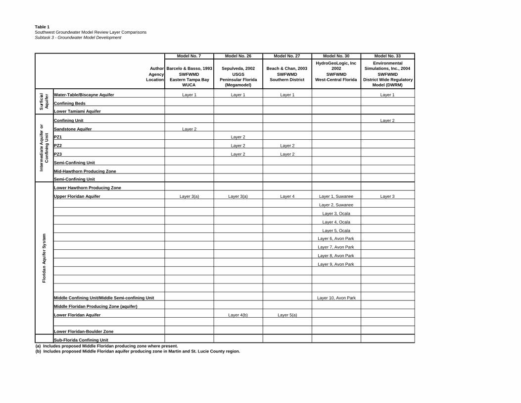
Table 1
Southwest Groundwater Model Review Layer Comparisons
Subtask 3 - Groundwater Model Development
Model No. 7 Model No. 26 Model No. 27 Model No. 30 Model No. 33
Author Barcelo & Basso, 1993 Sepulveda, 2002 Beach & Chan, 2003
HydroGeoLogic, Inc
2002
Environmental
Simulations, Inc., 2004
Agency SWFWMD USGS SWFWMD SWFWMD SWFWMD
Location Eastern Tampa Bay
WUCA
Peninsular Florida
(Megamodel)
Southern District West-Central Florida District Wide Regulatory
Model (DWRM)
Water-Table/Biscayne Aquifer Layer 1 Layer 1 Layer 1 Layer 1
Confining Beds
Lower Tamiami Aquifer
Confining Unit Layer 2
Sandstone Aquifer Layer 2
PZ1 Layer 2
PZ2 Layer 2 Layer 2
PZ3 Layer 2 Layer 2
Semi-Confining Unit
Mid-Hawthorn Producing Zone
Semi-Confining Unit
Lower Hawthorn Producing Zone
Upper Floridan Aquifer Layer 3(a) Layer 3(a) Layer 4 Layer 1, Suwanee Layer 3
Layer 2, Suwanee
Layer 3, Ocala
Layer 4, Ocala
Layer 5, Ocala
Layer 6, Avon Park
Layer 7, Avon Park
Layer 8, Avon Park
Layer 9, Avon Park
Middle Confining Unit/Middle Semi-confining Unit Layer 10, Avon Park
Middle Floridan Producing Zone (aquifer)
Lower Floridan Aquifer Layer 4(b) Layer 5(a)
Lower Floridan-Boulder Zone
Sub-Florida Confining Unit
(a) Includes proposed Middle Floridan producing zone where present.
(b) Includes proposed Middle Floridan aquifer producing zone in Martin and St. Lucie County region.
Sur
fic
ial
Aq
uif
er
Inte
rmed
iate
Aq
uif
ero
r
Co
nfi
nin
gU
nit
Flo
rid
an
Aq
uif
er
Sy
ste
m

FIGURES
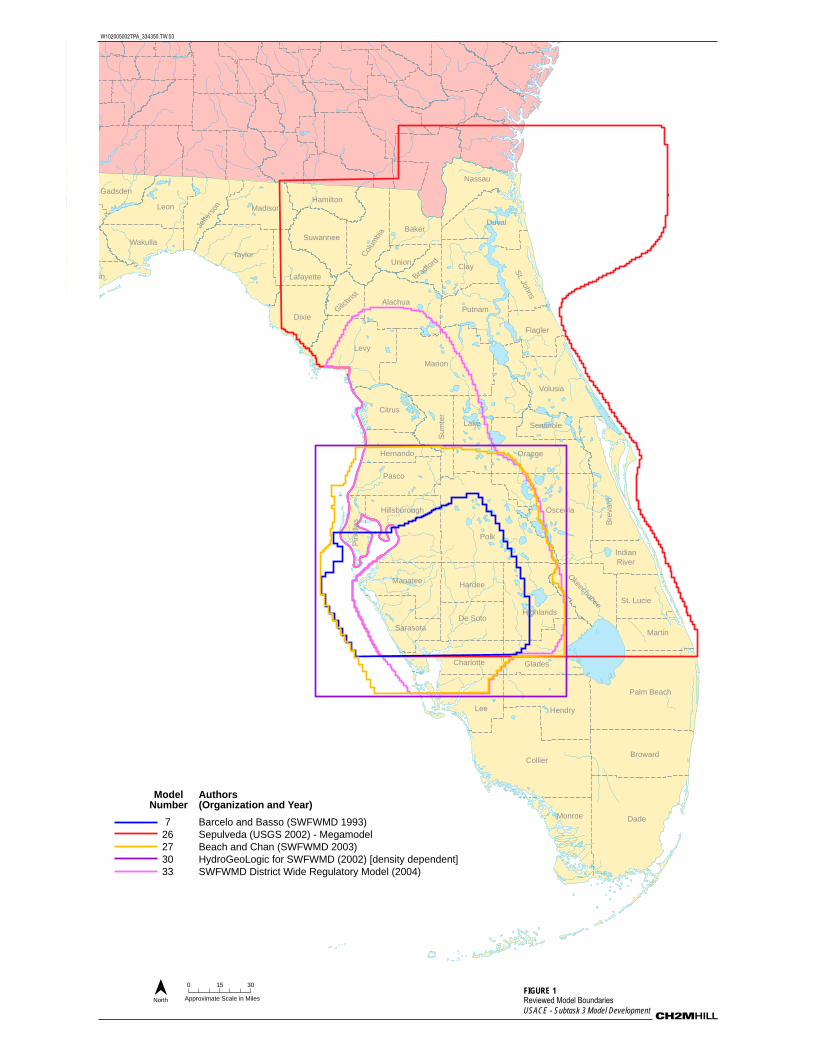
Franklin
Gadsden
Leon
Wakulla
Alachua
Baker
Bradfo
rd
Bre
vard
Broward
Charlotte
Citrus
Clay
Collier
Col
umbi
a
Dade
De Soto
Dixie
Duval
Flagler
Gilc
hrist
Glades
Hamilton
Hardee
Hendry
Hernando
Highlands
Hillsborough
Indian
River
Jeffe
rson
Lafayette
Lake
Lee
Levy
Madison
Manatee
Marion
Martin
Monroe
Okeechobee
Palm Beach
Pasco
Pin
ella
s
Polk
Putnam
St. Jo
hns
St. Lucie
Sarasota
Seminole
Sum
ter
Suwannee
TaylorUnion
Volusia
Liberty
Orange
Osceola
Nassau
W102005002TPA_334350.TW.03
North
FIGURE 1
Reviewed Model Boundaries
USACE - Subtask 3 Model Development
7
26
27
30
33
Barcelo and Basso (SWFWMD 1993)
Sepulveda (USGS 2002) - Megamodel
Beach and Chan (SWFWMD 2003)
HydroGeoLogic for SWFWMD (2002) [density dependent]
SWFWMD District Wide Regulatory Model (2004)
ModelNumber
Authors(Organization and Year)
0 3015
Approximate Scale in Miles
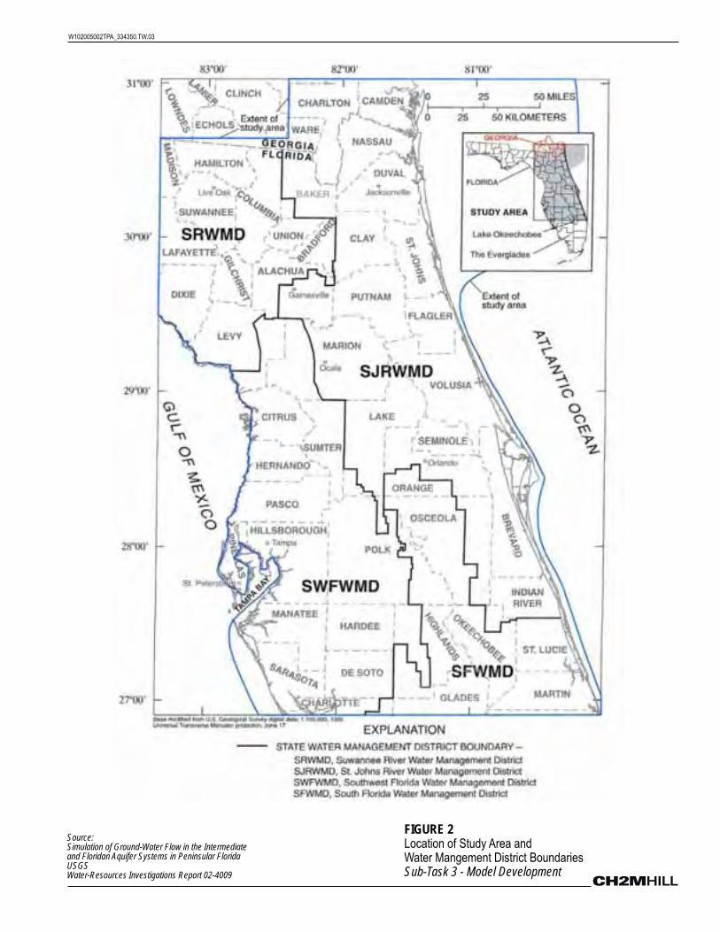
W102005002TPA_334350.TW.03
FIGURE 2
Location of Study Area andWater Mangement District BoundariesSub-Task 3 - Model Development
Source:Simulation of Ground-Water Flow in the Intermediateand Floridan Aquifer Systems in Peninsular FloridaUSGSWater-Resources Investigations Report 02-4009

W102005002TPA_334350.TW.03
FIGURE 3
Stratigraphic Units, General Lithology, and Hydrogeologic UnitsSub-Task 3 - Model Development
Source:Simulation of Ground-Water Flow in the Intermediateand Floridan Aquifer Systems in Peninsular FloridaUSGSWater-Resources Investigations Report 02-4009
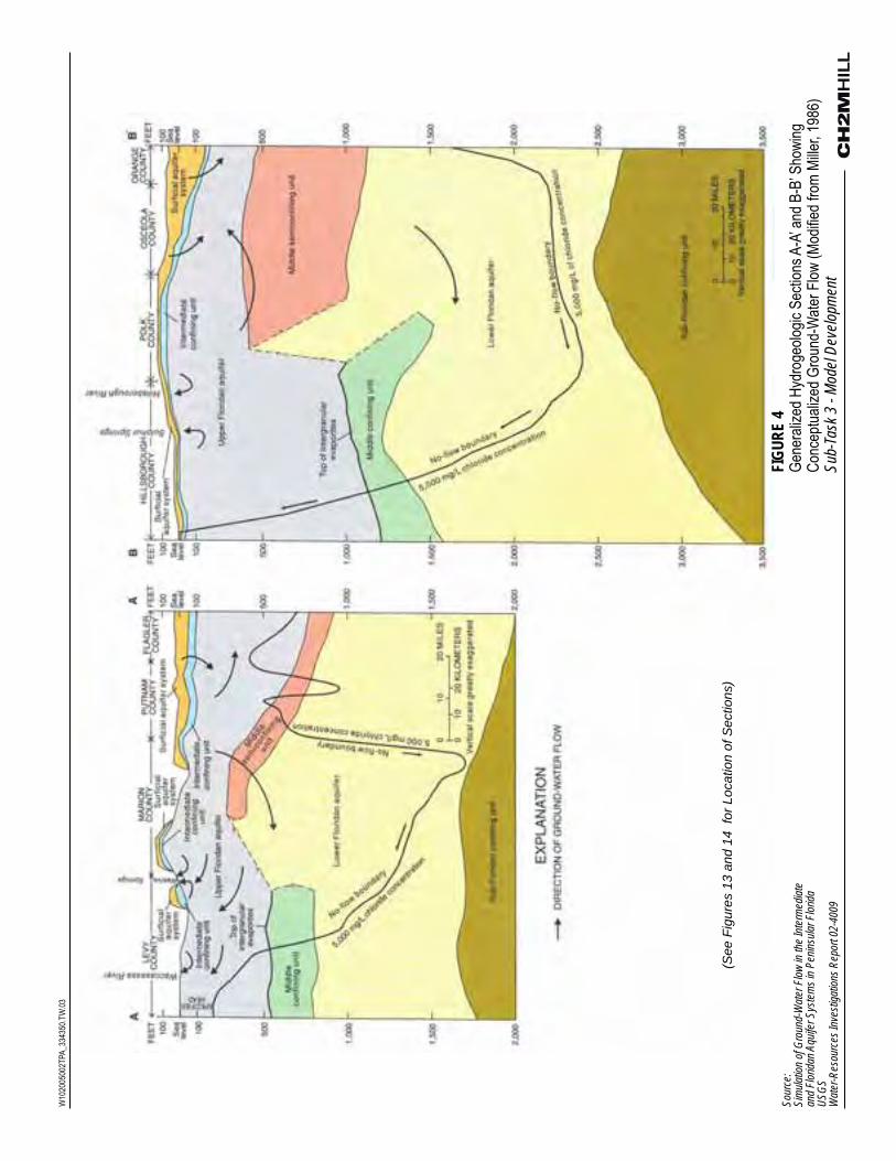
FIG
UR
E 4
Gen
eral
ized
Hyd
roge
olog
ic S
ectio
ns A
-A’ a
nd B
-B’ S
how
ing
Con
cept
ualiz
ed G
roun
d-W
ater
Flo
w (
Mod
ified
from
Mill
er, 1
986)
Sub
-Tas
k 3
- M
odel
Dev
elop
men
t
Sou
rce:
Sim
ulat
ion
of G
roun
d-W
ater
Flo
w in
the
Inte
rmed
iate
and
Flo
ridan
Aqu
ifer
Sys
tem
s in
Pen
insu
lar
Flo
rida
US
GS
Wat
er-R
esou
rces
Inve
stig
atio
ns R
epor
t 02-
4009
W10
2005
002T
PA
_334
350.
TW
.03
(See F
igure
s 1
3 a
nd 1
4 fo
r Location o
f S
ections)

FIG
UR
E 5
Laye
ring
Sch
eme
and
Rep
rese
ntat
ion
of G
eolo
gic
Uni
ts in
Loc
al M
odel
s 1
and
3, a
nd C
orre
spon
ding
La
yerin
g S
chem
e in
the
Reg
iona
l Mod
elS
ub-T
ask
3 -
Mod
el D
evel
opm
ent
Sou
rce:
Sim
ulat
ion
of G
roun
d-W
ater
Flo
w in
the
Inte
rmed
iate
and
Flo
ridan
Aqu
ifer
Sys
tem
s in
Pen
insu
lar
Flo
rida
US
GS
Wat
er-R
esou
rces
Inve
stig
atio
ns R
epor
t 02-
4009
W10
2005
002T
PA
_334
350.
TW
.03
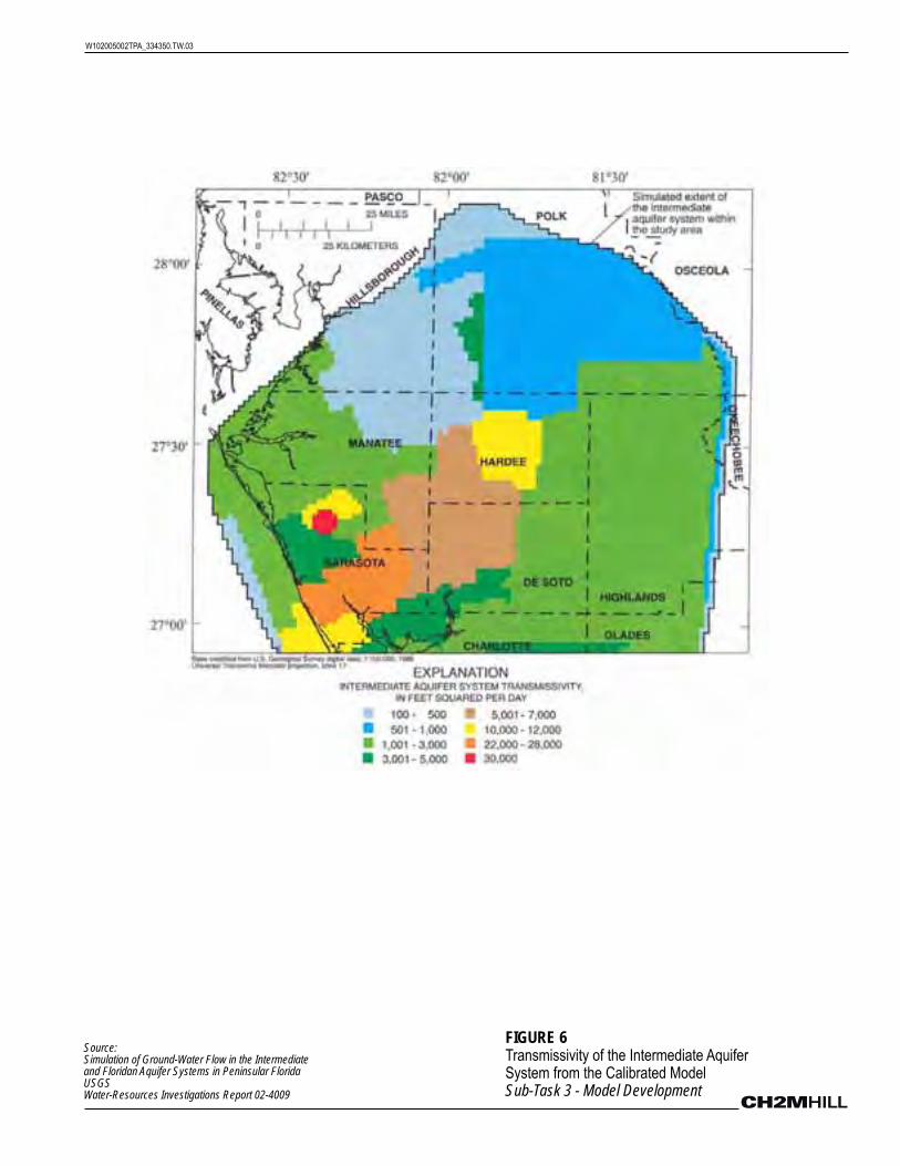
W102005002TPA_334350.TW.03
FIGURE 6
Transmissivity of the Intermediate Aquifer System from the Calibrated ModelSub-Task 3 - Model Development
Source:Simulation of Ground-Water Flow in the Intermediateand Floridan Aquifer Systems in Peninsular FloridaUSGSWater-Resources Investigations Report 02-4009
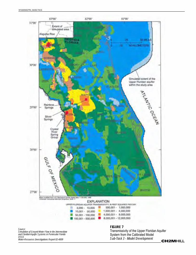
W102005002TPA_334350.TW.03
FIGURE 7
Transmissivity of the Upper Floridan Aquifer System from the Calibrated ModelSub-Task 3 - Model Development
Source:Simulation of Ground-Water Flow in the Intermediateand Floridan Aquifer Systems in Peninsular FloridaUSGSWater-Resources Investigations Report 02-4009
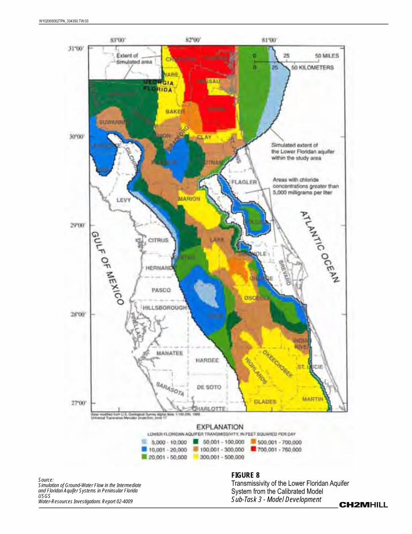
W102005002TPA_334350.TW.03
FIGURE 8
Transmissivity of the Lower Floridan Aquifer System from the Calibrated ModelSub-Task 3 - Model Development
Source:Simulation of Ground-Water Flow in the Intermediateand Floridan Aquifer Systems in Peninsular FloridaUSGSWater-Resources Investigations Report 02-4009
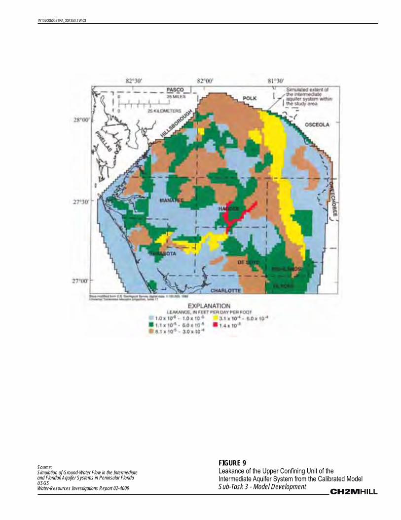
W102005002TPA_334350.TW.03
FIGURE 9
Leakance of the Upper Confining Unit of the Intermediate Aquifer System from the Calibrated ModelSub-Task 3 - Model Development
Source:Simulation of Ground-Water Flow in the Intermediateand Floridan Aquifer Systems in Peninsular FloridaUSGSWater-Resources Investigations Report 02-4009
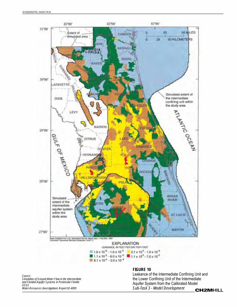
W102005002TPA_334350.TW.03
FIGURE 10
Leakance of the Intermediate Confining Unit and the Lower Confining Unit of the Intermediate Aquifer System from the Calibrated ModelSub-Task 3 - Model Development
Source:Simulation of Ground-Water Flow in the Intermediateand Floridan Aquifer Systems in Peninsular FloridaUSGSWater-Resources Investigations Report 02-4009

W102005002TPA_334350.TW.03
FIGURE 11
Leakance of the Middle Confining and Middle Semiconfining Units from the Calibrated ModelSub-Task 3 - Model Development
Source:Simulation of Ground-Water Flow in the Intermediateand Floridan Aquifer Systems in Peninsular FloridaUSGSWater-Resources Investigations Report 02-4009
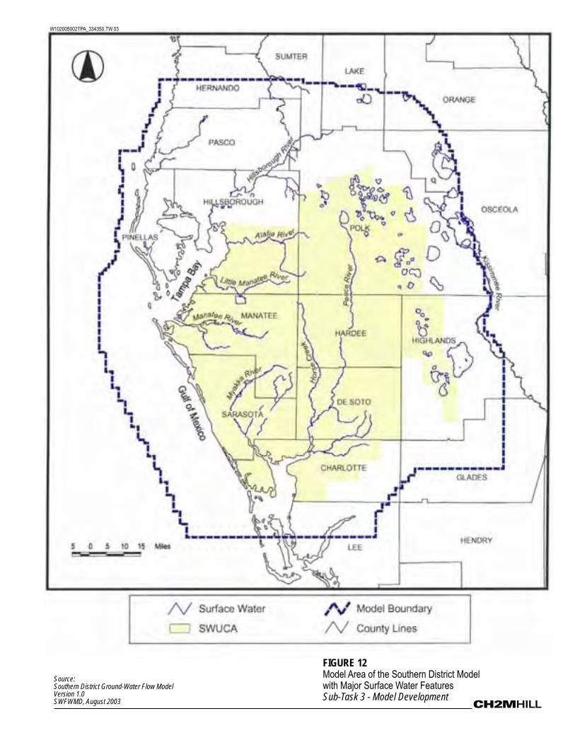
W102005002TPA_334350.TW.03
FIGURE 12
Model Area of the Southern District Model with Major Surface Water FeaturesSub-Task 3 - Model Development
Source:Southern District Ground-Water Flow ModelVersion 1.0SWFWMD, August 2003
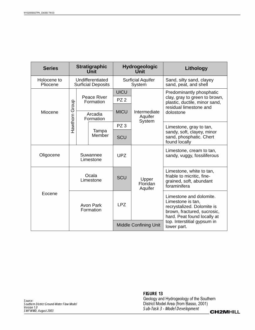
Series Lithology StratigraphicUnit
HydrogeologicUnit
Holocene to Pliocene
Undifferentiated Surficial Deposits
Surficial Aquifer System
Sand, silty sand, clayey sand, peat, and shell
Predominantly phosphatic clay, gray to green to brown, plastic, ductile, minor sand, residual limestone and dolostone
Limestone, gray to tan, sandy, soft, clayey, minor sand, phosphatic. Chert found locally
Limestone, white to tan, friable to micritic, fine- grained, soft, abundant foraminifera
Limestone, cream to tan, sandy, vuggy, fossiliferous
Peace River Formation
IntermediateAquiferSystem
UpperFloridanAquifer
Middle Confining Unit
ArcadiaFormation
Tampa Member
SuwanneeLimestone
OcalaLimestone
Avon Park Formation
Miocene
Oligocene
Eocene
Haw
thorn
Gro
up
UICU
MICU
SCU
SCU
UPZ
LPZ
PZ 2
PZ 3
Limestone and dolomite. Limestone is tan, recrystalized. Dolomite is brown, fractured, sucrosic, hard. Peat found locally at top. Interstitial gypsum in lower part.
FIGURE 13
Geology and Hydrogeology of the Southern District Model Area (from Basso, 2001)Sub-Task 3 - Model Development
W102005002TPA_334350.TW.03
Source:Southern District Ground-Water Flow ModelVersion 1.0SWFWMD, August 2003

FIGURE 14
Conceptual Model as Hydrogeologic Cross Section from East to West (Section A-A’)Sub-Task 3 - Model Development
W102005002TPA_334350.TW.03
Source:Southern District Ground-Water Flow ModelVersion 1.0SWFWMD, August 2003
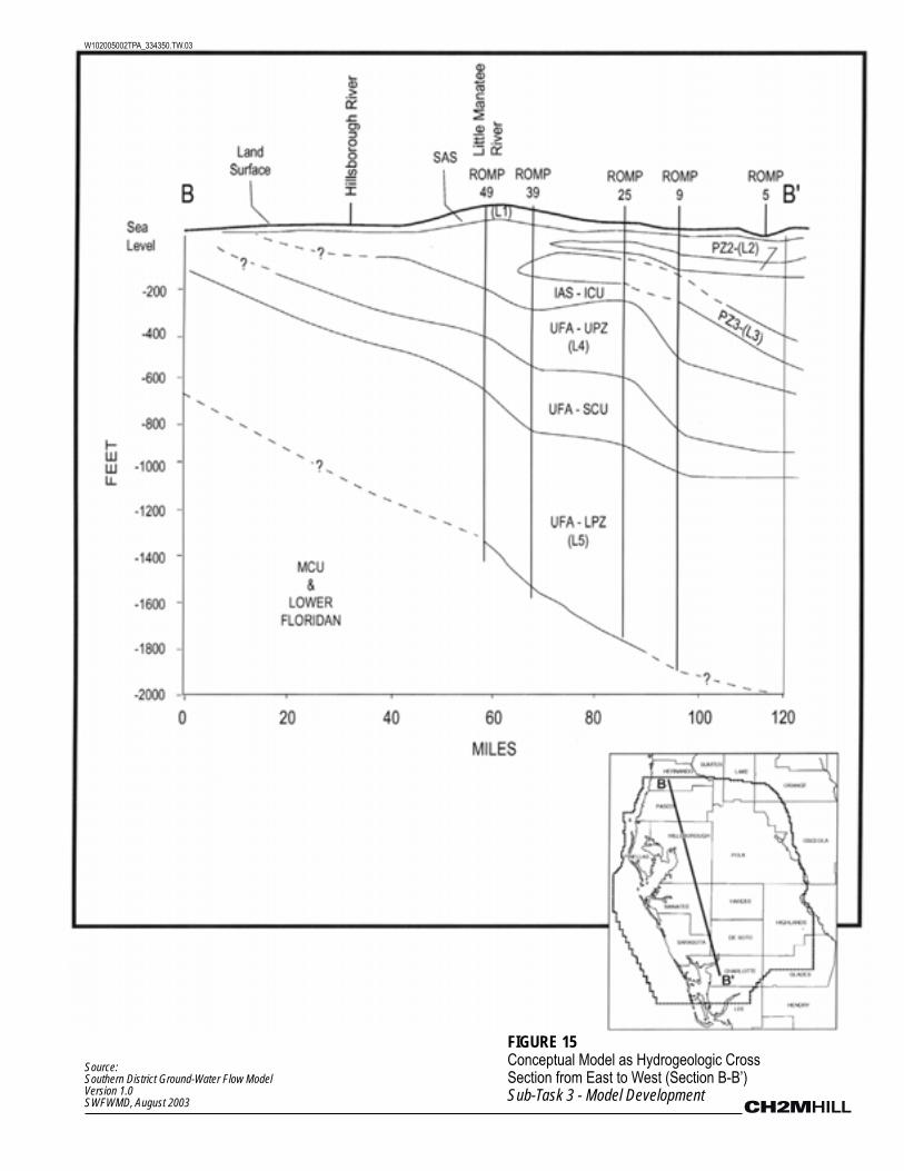
FIGURE 15
Conceptual Model as Hydrogeologic Cross Section from East to West (Section B-B’)Sub-Task 3 - Model Development
W102005002TPA_334350.TW.03
Source:Southern District Ground-Water Flow ModelVersion 1.0SWFWMD, August 2003

FIGURE 16
Calibrated Transmissivity Distributions with Field Observed Values: Layer 2Sub-Task 3 - Model Development
W102005002TPA_334350.TW.03
Source:Southern District Ground-Water Flow ModelVersion 1.0SWFWMD, August 2003
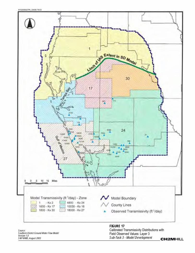
FIGURE 17
Calibrated Transmissivity Distributions with Field Observed Values: Layer 3Sub-Task 3 - Model Development
W102005002TPA_334350.TW.03
Source:Southern District Ground-Water Flow ModelVersion 1.0SWFWMD, August 2003

FIGURE 18
Calibrated Transmissivity Distributions with Field Observed Values: Layer 4Sub-Task 3 - Model Development
W102005002TPA_334350.TW.03
Source:Southern District Ground-Water Flow ModelVersion 1.0SWFWMD, August 2003
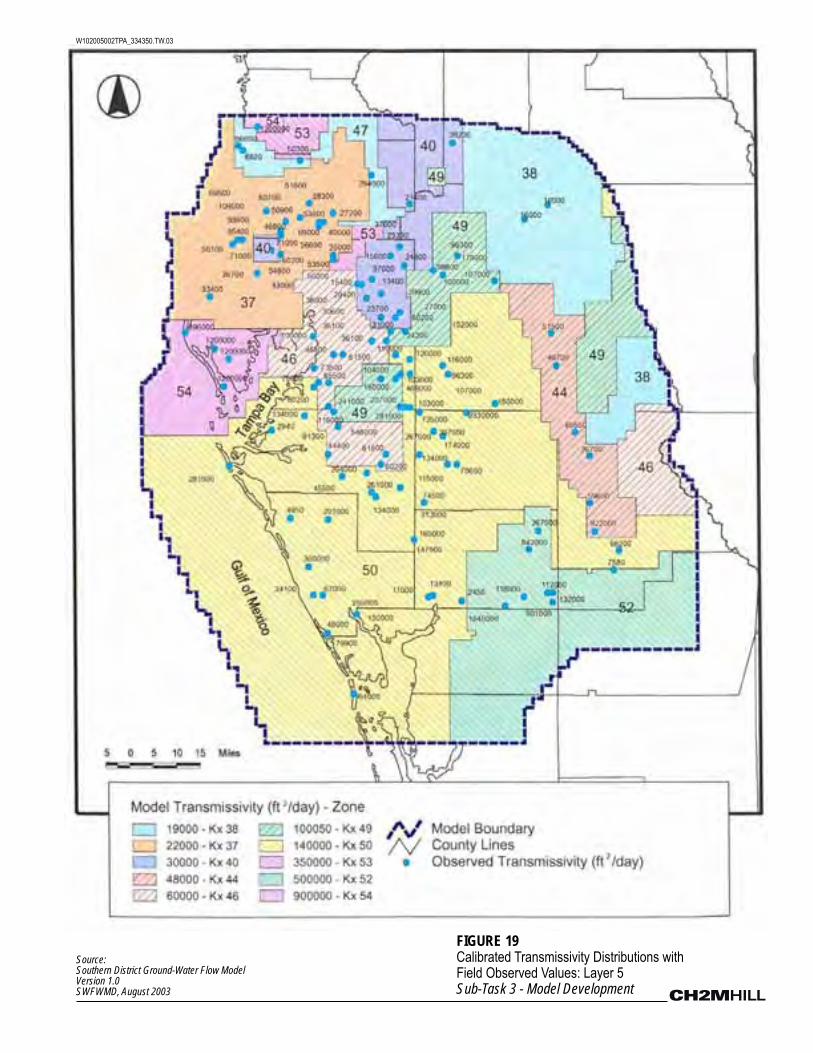
FIGURE 19
Calibrated Transmissivity Distributions with Field Observed Values: Layer 5Sub-Task 3 - Model Development
W102005002TPA_334350.TW.03
Source:Southern District Ground-Water Flow ModelVersion 1.0SWFWMD, August 2003
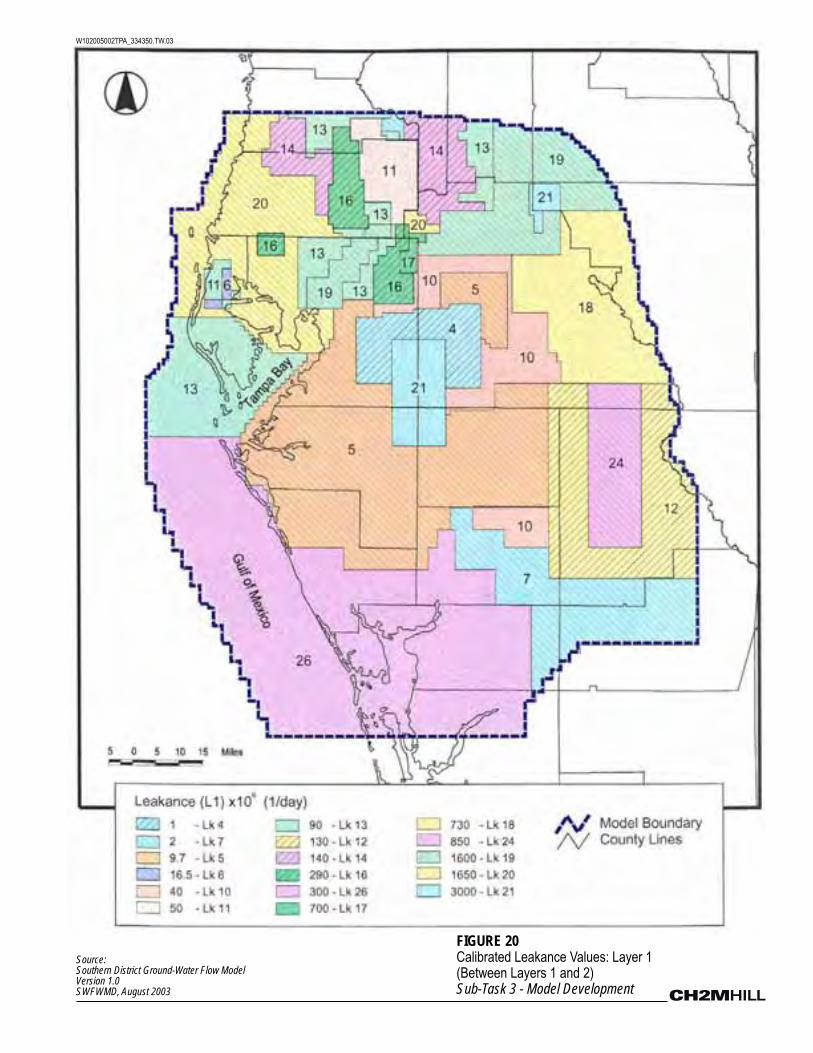
FIGURE 20
Calibrated Leakance Values: Layer 1 (Between Layers 1 and 2)Sub-Task 3 - Model Development
W102005002TPA_334350.TW.03
Source:Southern District Ground-Water Flow ModelVersion 1.0SWFWMD, August 2003
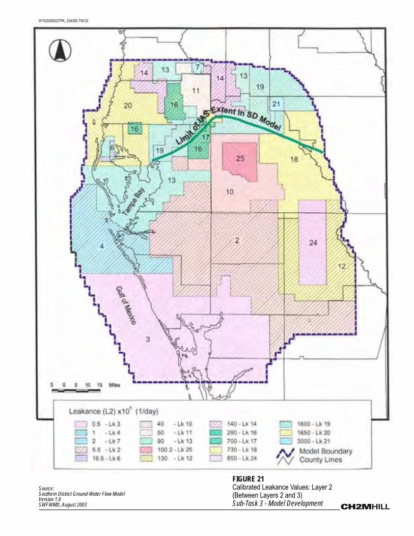
FIGURE 21
Calibrated Leakance Values: Layer 2 (Between Layers 2 and 3)Sub-Task 3 - Model Development
W102005002TPA_334350.TW.03
Source:Southern District Ground-Water Flow ModelVersion 1.0SWFWMD, August 2003
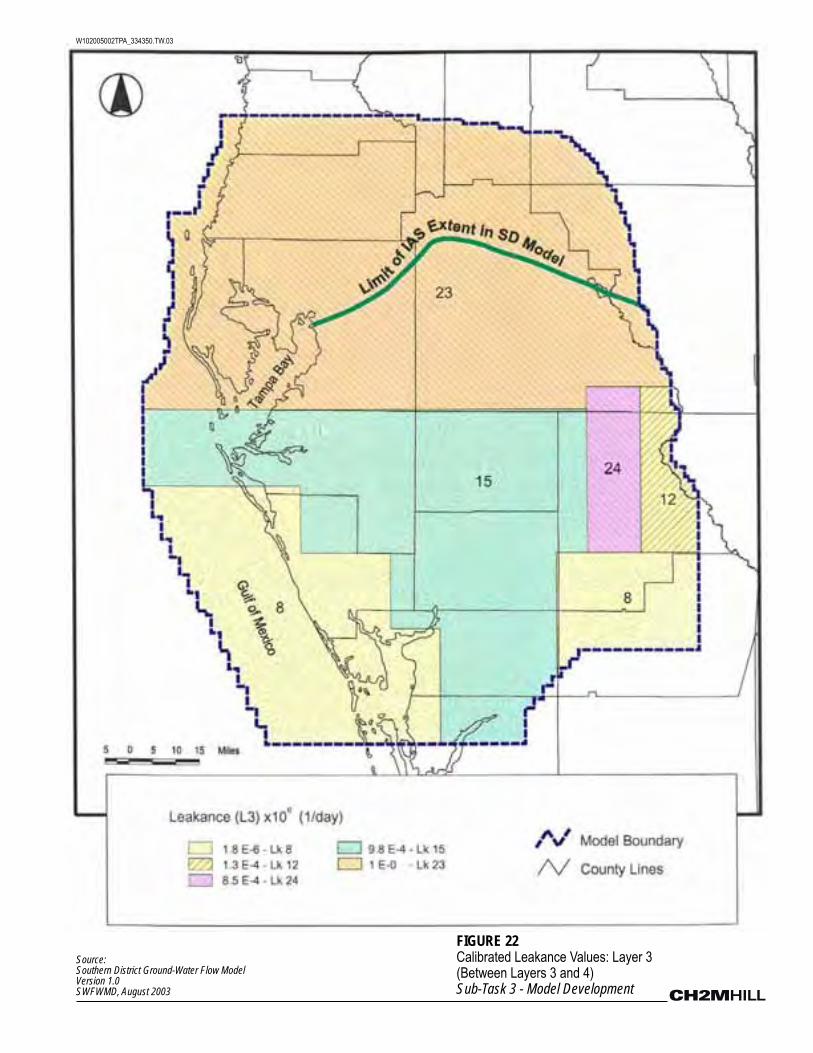
FIGURE 22
Calibrated Leakance Values: Layer 3 (Between Layers 3 and 4)Sub-Task 3 - Model Development
W102005002TPA_334350.TW.03
Source:Southern District Ground-Water Flow ModelVersion 1.0SWFWMD, August 2003
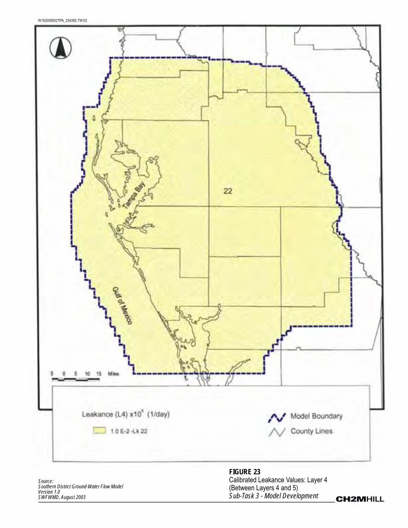
FIGURE 23
Calibrated Leakance Values: Layer 4 (Between Layers 4 and 5)Sub-Task 3 - Model Development
W102005002TPA_334350.TW.03
Source:Southern District Ground-Water Flow ModelVersion 1.0SWFWMD, August 2003

APPENDIX B
Southeast Florida Region Model Review TM
TPA/053320008/SOUTHEAST MODEL TM_07_2006_REV1.DOC 1
T E C H N I C A L M E M O R A N D U M
Southeast Florida Region Groundwater ModelReview: Fairbank et al. (1999), McGurk and Presley(2002), and Bower et al. (1990)
PREPARED FOR: USACE Jacksonville District
PREPARED BY: CH2M HILL
DATE: November 21, 2005
PROJECT NUMBER: 334350.TW.03
Contents
Introduction and Purpose ............................................................................................................1
Comparison of Hydrogeology and Model Frameworks .........................................................2Model Summaries..........................................................................................................................3
Lower East Coast Floridan Aquifer Model (Fairbank et al., 1999) ............................3
East-Central Floridan Aquifer Model (McGurk and Presley, 2002)..........................5
Lee County Model (Bower et al., 1990)..........................................................................7Model Comparison toHydrogeologic Framework ..................................................................9
References.....................................................................................................................................10Appendix A Selected Figures from Documentation of Lower East Coast Florida model
Appendix B Selected Figures and Tables from Documentation of the East
Coast Florida modelAppendix C Selected Figures from documentation of the Lee County, Florida model
Introduction and Purpose
The goal of this project is to collect and summarize data from available model
documentation and provide recommendations to the U.S. Army Corps of Engineers
(USACE) Jacksonville District for the development of a Regional Groundwater Model ofFlorida. This Technical Memorandum (TM) summarizes the model reviews for middle and
southern Florida.
Three models were reviewed. These models covered themiddle and southern part of the
Florida peninsula. Figure 1 shows the extent of the individual models. These models arereferenced in this TM as follows:
Lower East Coast Floridan Aquifer Model (Fairbank et al., 1999)
East-Central Floridan Aquifer Model (McGurk and Presley, 2002)
Lee County Model (Bower et al., 1990)
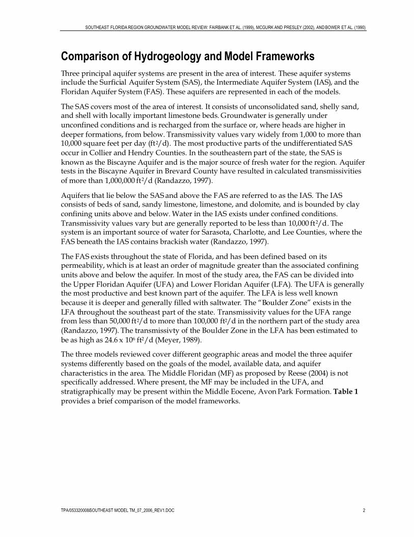
SOUTHEAST FLORIDA REGION GROUNDWATER MODEL REVIEW: FAIRBANK ET AL. (1999), MCGURK AND PRESLEY (2002), AND BOWER ET AL. (1990)
TPA/053320008/SOUTHEAST MODEL TM_07_2006_REV1.DOC 2
Comparison of Hydrogeology and Model Frameworks
Three principal aquifer systems are present in the area of interest. These aquifer systemsinclude the Surficial Aquifer System (SAS), the Intermediate Aquifer System (IAS), and the
Floridan Aquifer System (FAS). These aquifers are represented in each of the models.
The SAS covers most of the area of interest. It consists of unconsolidated sand, shelly sand,and shell with locally important limestone beds. Groundwater is generally under
unconfined conditions and is recharged from the surface or, where heads are higher in
deeper formations, from below. Transmissivity values vary widely from 1,000 to more than10,000 square feet per day (ft2/d). The most productive parts of the undifferentiated SAS
occur in Collier and Hendry Counties. In the southeastern part of the state, the SAS is
known as the Biscayne Aquifer and is the major source of fresh water for the region. Aquifertests in the Biscayne Aquifer in Brevard County have resulted in calculated transmissivities
of more than 1,000,000 ft2/d (Randazzo, 1997).
Aquifers that lie below the SAS and above the FAS are referred to as the IAS. The IASconsists of beds of sand, sandy limestone, limestone, and dolomite, and is bounded by clay
confining units above and below.Water in the IAS exists under confined conditions.
Transmissivity values vary but are generally reported to be less than 10,000 ft2/d. Thesystem is an important source of water for Sarasota, Charlotte, and Lee Counties, where the
FAS beneath the IAS contains brackish water (Randazzo, 1997).
The FAS exists throughout the state of Florida, and has been defined based on itspermeability, which is at least an order of magnitude greater than the associated confining
units above and below the aquifer. In most of the study area, the FAS can be divided into
the Upper Floridan Aquifer (UFA) and Lower Floridan Aquifer (LFA). The UFA is generallythe most productive and best known part of the aquifer. The LFA is less well known
because it is deeper and generally filled with saltwater. The “Boulder Zone” exists in the
LFA throughout the southeast part of the state. Transmissivity values for the UFA rangefrom less than 50,000 ft2/d to more than 100,000 ft2/d in the northern part of the study area
(Randazzo, 1997). The transmissivty of the Boulder Zone in the LFA has been estimated to
be as high as 24.6 x 106 ft2/d (Meyer, 1989).
The three models reviewed cover different geographic areas and model the three aquifer
systems differently based on the goals of the model, available data, and aquifer
characteristics in the area. The Middle Floridan (MF) as proposed by Reese (2004) is notspecifically addressed.Where present, the MF may be included in the UFA, and
stratigraphically may be present within the Middle Eocene, AvonPark Formation. Table 1
provides a brief comparison of the model frameworks.

SOUTHEAST FLORIDA REGION GROUNDWATER MODEL REVIEW: FAIRBANK ET AL. (1999), MCGURK AND PRESLEY (2002), AND BOWER ET AL. (1990)
TPA/053320008/SOUTHEAST MODEL TM_07_2006_REV1.DOC 3
TABLE 1Comparison of Model Frameworks
Southeast Florida Region Model Review
Layer Lower East Coast East Central Florida Lee County
Layer 1 Surficial Aquifer System Surficial Aquifer System Surficial Aquifer System (Water
Table)
Layer 2 Semi Confining Units Upper Floridan (Avon Park,Ocala)
Surficial Aquifer System (LowerTamiami Aquifer)
Layer 3 Upper Floridan (Avon Park,Ocala)
Upper Floridan (Avon Park)* Intermediate Aquifer System(Sandstone Aquifer)
Layer 4 Semi Confining Units Lower Floridan Intermediate Aquifer System
(Mid-Hawthorn Aquifer)
Layer 5 Upper Floridan (Avon Park)* Floridian Aquifer System (Lower
Hawthorn Aquifer)
Layer 6 Semi Confining Units Floridian Aquifer System (Suwanneeand Deeper Aquifers)
Layer 7 Lower Floridan (Oldsmar) Floridian Aquifer System (Suwanneeand Deeper Aquifers)
Layer 8 Semi Confining Units
Layer 9 Base of Floridan (BoulderZone)
* included proposed MF where present
Model Summaries
Lower East Coast Floridan Aquifer Model (Fairbank et al., 1999)
Conceptual Model
A three-dimensional, steady-state model was created for the Lower East Coast Planning
Area. Appendix A provides figures from the model documentation. The model includesthree primary flow zones; two arewithin the UFA and a third is in the LFA. Flow Zone 1
includes permeable zones at or near the top of the Avon Park Formation and the Ocala
Limestone (Layer 3). Flow Zone 2 includes permeable zones within the upper part of theAvon Park Formation (Layer 5) and includes the MF where present. Flow Zone 3 includes
the shallowest producing intervals at or near the top of the Oldsmar Formation (Layer 7).
Low permeability units between the primary flow zones are included explicitly in thismodel. Additionally, the SAS and the Boulder Zone are included as constant head
boundaries at the top and bottom of the model, respectively. Figure 2 in Appendix A
provides the Flow Zone Conceptualization.
Numerical Model
Model Grid Description
Based on the available documentation, the model covers 16,434 square miles and has a total
of nine layers with a uniform grid spacing of 1 mile. The model grid domain is shown in
Figure 1 in Appendix A.

SOUTHEAST FLORIDA REGION GROUNDWATER MODEL REVIEW: FAIRBANK ET AL. (1999), MCGURK AND PRESLEY (2002), AND BOWER ET AL. (1990)
TPA/053320008/SOUTHEAST MODEL TM_07_2006_REV1.DOC 4
Range of Hydraulic Conductivity and Transmissivity
Table 2 presents horizontal and vertical hydraulic conductivity values reported in the modeldocumentation. Variable layer thickness resulted in variable values of transmissivity.
Sensitivity analysis of the model to values of hydraulic conductivity in the model layers is
included in the model documentation.
TABLE 2
Model Layers and Hydraulic Conductivity ValuesSoutheast Florida Region Model Review
Horizontal K Vertical K
Layer Formation Layer Type (ft/day) (ft/day)
Layer 1 Surficial Aquifer System Constant Head N/A N/A
Layer 2 Semi Confining Units Leakance Layer 0.5 1.0 e-5
Layer 3 Upper Floridan (Avon Park, Ocala) Active Layer 175 8.0
Layer 4 Semi Confining Units Leakance Layer 0.09 7.0 e-3
Layer 5 Upper Floridan (Avon Park)* Active Layer 75 9.0
Layer 6 Semi Confining Units Leakance Layer 9 2.2 e-3
Layer 7 Lower Floridan (Oldsmar) Active Layer 99 2.2 e-4
Layer 8 Semi Confining Units Leakance Layer 0.9 1.7 e-3
Layer 9 Base of Floridan (Boulder Zone) Constant Head N/A N/A
* includes proposed MF where present
Layer thickness varied based on contact elevations collected from test borings and wells
drilled in the study area. Table 1 included in Appendix A provides the data used for layerelevations. Hydrostratigraphic picks for model layers are based on data compiled from
reports prepared by consultants and SFWMD. The model documentation provides an
extensive list of well/test drilling sites and layer elevations.
Recharge
Recharge is not explicitlymodeled. Instead, Layer 1 is modeled as a constant head boundary
condition which supplies recharge or allows discharge through the semiconfining Layer 2.
Boundary Conditions
The top and bottom layers (Layer 1 and Layer 9) are modeled as constant head boundaries
which supply recharge or allows discharge of groundwater through the associated
semiconfining units. General head boundaries are utilized laterally around the modeldomain. Figures 4 and 10 in Appendix A show the locations of model boundaries. The
constant head value for Layer 1 was calculated to be 2.5 feet from existing land surface. Lake
Okeechobee was modeled at 15.4 feet which represents the average stage for the period ofrecord. Starting head and boundary conditions for lower layers were created using pressure
data from the SFWMDmonitoring well network and FDEP monitoringwells. A total of 26
District wells and 47 utility wells were used to gather information. Figures 4 through 10 inAppendix A show initial head distributions.
SOUTHEAST FLORIDA REGION GROUNDWATER MODEL REVIEW: FAIRBANK ET AL. (1999), MCGURK AND PRESLEY (2002), AND BOWER ET AL. (1990)
TPA/053320008/SOUTHEAST MODEL TM_07_2006_REV1.DOC 5
Applied Stresses
Only two prescribed flow conditions (pumping wells) are included in the model. Averagevalues of pumping for the Boynton Beach ASR facility and the Jupiter reverse osmosis (RO)
facility were used during calibration of the model. Figure 3 in Appendix A shows the
locations of the pumping facilities included in the model.
Calibration
The steady-state calibration period for the model is from 1995 to 1997. Two facilities
operated continuously during this period and were included in the model: the Boynton
Beach ASR facility and the Jupiter RO facility. Initial values for aquifer parameters werebased on representative values collected from wells completed in the intervals included in
the model. Table 2 in Appendix A provides the basis for the parameters. Table 10 inAppendix A compares the calculated and model calibrated values.
Water quality in the FAS in the area of the model varies, causing density differences which
affect groundwater flow. The model utilizes “fresh-water equivalent head values” to
account for this water quality variation.
East-Central Floridan Aquifer Model (McGurk and Presley, 2002)
Conceptual Model
A three-dimensional steady-state model was created, expanding on previous regional
models covering all or parts of Orange, Seminole, Brevard, Lake, Osceola, Marion, Polk,
Sumter, and Volusia Counties. Appendix B provides figures from the model documentation.Figures 1 and 2 in Appendix B show the location of the modeled area. The model was
created to simulate pre-development conditions, modern day post-development conditions,
and future flow conditions which incorporate increased water supply demands.
The SAS, the Intermediate Confining Unit (ICU), and the FAS are simulated. The SAS
consists of sand, silt, clayey sand, and shell beds, and receives recharge from rainfall,
irrigation water, septic tank effluent, rapid infiltration basins and other sources. The ICUseparates the SAS from the FAS. The thickness of the confining unit and its hydrogeologic
properties are highly variable. The FAS includes the Oldsmar Formation, Avon Park
Formation, and the Ocala Limestone. The FAS is separated into the UFA, the middlesemiconfining unit, and the LFA. Figure 7 in Appendix B provides the geologic and
hydrostratigraphic units within the project area. Figure 25 in Appendix B shows a cross
section with the units and direction of saline and fresh groundwater flow.
Numerical Model
Model Grid Description
The model covers 7,568 square miles. The grid is uniform with 2,500-foot by 2,500-foot
square cells. Layer elevations were calculated based on data from data collected fromprevious studies and an extensive list of wells and test borings is included in the appendix
of themodel documentation. Figures 4 and 5 in Appendix B show the locations of wells
completed in the SAS and FAS utilized for this study. Figures 9 through 14 in Appendix B
show layer elevations within the model. At cell locations where the saline water interface

SOUTHEAST FLORIDA REGION GROUNDWATER MODEL REVIEW: FAIRBANK ET AL. (1999), MCGURK AND PRESLEY (2002), AND BOWER ET AL. (1990)
TPA/053320008/SOUTHEAST MODEL TM_07_2006_REV1.DOC 6
elevation was calculated to be above an aquifer layer bottom elevation, the bottom elevation
of the flow domain was recomputed to equal the saline water interface elevation. Cellswhere the saline water interface was calculated to be within 20 feet of the top of an aquifer
layer were considered to be saline and therefore inactive.
Range of Hydraulic Conductivity and Transmissivity
The model includes variable values of hydraulic conductivity and associated transmissivity.
Figure 8 in Appendix B provides the locations of aquifer performance tests completed in the
study area. Table 3 provides the ranges reported. Additionally, Figures 65 through 76 inAppendix B show the spatial distribution of the aquifer parameters.
TABLE 3Model Layers and Hydraulic Conductivity Values
Southeast Florida Region Model Review
Horizontal K Vertical K
Layer Formation Layer Type (ft/day) (ft/day)
Layer 1 Surficial Aquifer System Unconfined Active 20 0.001 - 0.1
Layer 2 Upper Floridan (Avon Park, Ocala) Confined Active 50-5000 0.25-50
Layer 3 Upper Floridan (Avon Park) Confined Active 50-5000 0.01 – 1.5
Layer 4 Lower Floridan Confined Active 15-500
* includes proposed MF where present
Recharge
The model utilizes the recharge package to apply recharge to the SAS based on detailed
information including precipitation, water applied to rapid infiltration basins, septic tankeffluent, and irrigation.
Boundary Conditions
General head boundaries are utilized laterally around the model. The head values are basedon estimated predevelopment heads in Layers 2 and 3. Layer 4, the LFA, generally varied
from +2 feet to -2 feet from the upper layer elevations depending on known
discharge/recharge zones. An exception is noted in the southwest where it was 10 to 20 feetlower based on local data. Figure 28 in Appendix B shows modeled lateral boundaries.
General head boundaries were also used to simulate the water level and flux changes along
the seaward boundary between saltwater and freshwater within the interior of the grid. Thisboundary condition was selected to allow for changes due to the moving transition zone.
Lakes, rivers, and other surface water attributes were modeled as constant heads cells and
rivers as appropriate.
Applied Stresses
Drainage wells provide significant man made source of recharge to the FAS. These injection
wells are numerous in the model. Injection rates were based on detailed evaluation ofinjection well locations and types from available reports. Pumping wells are shown in
Figures 30 through 32 of Appendix B for each of the model layers.
SOUTHEAST FLORIDA REGION GROUNDWATER MODEL REVIEW: FAIRBANK ET AL. (1999), MCGURK AND PRESLEY (2002), AND BOWER ET AL. (1990)
TPA/053320008/SOUTHEAST MODEL TM_07_2006_REV1.DOC 7
Calibration
The model was calibrated to average 1995 steady-state conditions. Calibration includedcomparison of observed and modeled groundwater levels as well as evaluation of stream
flow and spring flow data.
Data utilized to create this detailed model came from many sources. Rainfall, surface waterdata, observation and test well data, groundwater withdrawal data, wastewater treatment
plant flows, and reuse data were obtained from agencies and reports on previous models
and studies. An extensive appendix (more than 400 pages) provided with the modeldocumentation contains much of this information.
Lee County Model (Bower et al., 1990)
Conceptual Model
The Lee County Model was created to be used for predictive purposes when evaluating
requests for large groundwater withdrawals and to serve as a basis for groundwater
management planning in Lee County. The three aquifer systems within the study area arethe SAS (including the water table and lower Tamiami aquifers), the IAS (including the
sandstone andMid-Hawthorn and associated confining units), and the FAS (including thelower Hawthorn and collectively the Suwannee and deeper aquifers). In the study area, the
FAS contains water with salinity levels above recommended standards for potable use.
Figure 1 in Appendix C shows the location of the study area. Figure 2 in Appendix C
provides the generalized hydrogeologic cross section. Figure 3 in Appendix C provides across section showing aquifers and corresponding model layers.
Numerical Model
Model Grid Resolution
The model extends across Lee County and covers more than 2,000 square miles. The modelconsists of 42 rows and 48 columns. Cells in the interior of the model are 1 mile square. Cells
on the north and west sides of the model were expanded to reduce boundary effects seen
during early calibration attempts. Figures 5 and 6 in Appendix C show the model domainand grid.
Range of Hydraulic Conductivity and Transmissivity
Values for transmissivity were variable for all layers except Layer 6. Figures A-38 through
A-54 provide areal distribution of hydraulic parameters included in the model. Table 4contains the approximate ranges taken from these figures. Vertical conductance (Vcon) is
substituted for vertical conductivity to be consistent with the model documentation. Verticalhydraulic conductivity can be calculated from the Vcon values by multiplying them by the
confining layer thickness. However, these data are not available in the documentation.
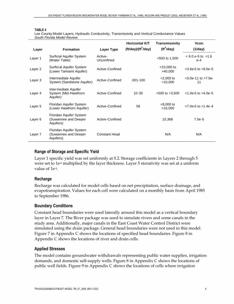
SOUTHEAST FLORIDA REGION GROUNDWATER MODEL REVIEW: FAIRBANK ET AL. (1999), MCGURK AND PRESLEY (2002), AND BOWER ET AL. (1990)
TPA/053320008/SOUTHEAST MODEL TM_07_2006_REV1.DOC 8
TABLE 4Lee County Model Layers, Hydraulic Conductivity, Transmissivity and Vertical Conductance ValuesSouth Florida Model Review
Horizontal K/T Transmissivity Vcon
Layer Formation Layer Type (ft/day)/(ft2/day) (ft
2/day) (1/day)
Layer 1Surficial Aquifer System(Water Table)
Active-Unconfined
<500 to 1,500< 6.0 e-5 to >1.6
e-4
Layer 2Surficial Aquifer System
(Lower Tamiami Aquifer)Active-Confined
<10,000 to
>40,000<3.6e-5 to >9.0e-5
Layer 3Intermediate AquiferSystem (Sandstone Aquifer)
Active-Confined .001-100<2,000 to>10,000
<3.0e-11 to >7.5e-11
Layer 4Intermediate AquiferSystem (Mid-HawthornAquifer)
Active-Confined 10-30 <500 to >3,500 <1.0e-5 to >4.0e-5
Layer 5Floridan Aquifer System(Lower Hawthorn Aquifer)
Active-Confined 56<8,000 to>16,000
<7.0e-5 to >1.4e-4
Layer 6
Floridan Aquifer System
(Suwannee and DeeperAquifers)
Active-Confined 10,368 7.0e-5
Layer 7
Floridan Aquifer System
(Suwannee and DeeperAquifers)
Constant Head N/A N/A
Range of Storage and Specific Yield
Layer 1 specific yield was set uniformly at 0.2. Storage coefficients in Layers 2 through 5were set to 1e-6 multiplied by the layer thickness. Layer 5 storativity was set at a uniform
value of 1e-4.
Recharge
Recharge was calculated for model cells based on net precipitation, surface drainage, andevapotranspiration. Values for each cell were calculated on amonthly basis from April 1985
to September 1986.
Boundary Conditions
Constant head boundaries were used laterally around this model as a vertical boundary
layer in Layer 7. The River package was used to simulate rivers and some canals in the
study area. Additionally, major canals in the East Coast Water Control District weresimulated using the drain package. General head boundaries were not used in this model.
Figure 7 in Appendix C shows the locations of specified head boundaries. Figure 8 in
Appendix C shows the locations of river and drain cells.
Applied Stresses
The model contains groundwater withdrawals representing public water supplies, irrigation
demands, and domestic self-supply wells. Figure 8 in Appendix C shows the locations ofpublic well fields. Figure 9 in Appendix C shows the locations of cells where irrigation

SOUTHEAST FLORIDA REGION GROUNDWATER MODEL REVIEW: FAIRBANK ET AL. (1999), MCGURK AND PRESLEY (2002), AND BOWER ET AL. (1990)
TPA/053320008/SOUTHEAST MODEL TM_07_2006_REV1.DOC 9
withdrawals are applied to the model. Figure 12 in Appendix C shows locations where
domestic self supply is included in the model.
Calibration
Both steady-state and transient calibrations were performed. The steady state run was used
as a starting point for the transient run. The transient model run was from April 1985 toSeptember 1986. The 12-month period from October 1985 to September 1986 was used for
calibration.
Model Comparison to Hydrogeologic Framework
The aquifer parameters taken from the models were compared to the values in the
hydrogeologic framework document. The greatest source of uncertainty in this evaluation is
the comparison of values for theMF, which is not explicitly described in the documentationof these models. Where there are two flow zones modeled in the UFA, the lower zone may
correspond to the proposed MF. Tables 5, 6, and 7 below compare the values.
TABLE 5
Lower East Coast Floridan Model – Comparison to Hydrogeologic FrameworkSoutheast Florida Region Model Review
Aquifer Hydrogeologic Parameter Average Framework Value(ft2/d)
Approx Model Range(ft2/d)
UF Transmissivity 24,911 2,800-82,600
MF Transmissivity 109,517 1,900-29,500*
LF Transmissivity 63,164 3,100-32,400
UF Storativity 1.15E-03 NA
MF Storativity 5.05E-03 NA
Middle Confining Unit 1 2.52E-01 7.00E-03
Middle Confining Unit 2 7.52E-01 2.20E-03
* Aquifers below Suwannee limestone
TABLE 6East Central Floridan Model – Comparison to Hydrogeologic Framework
Southeast Florida Region Model Review
Aquifer Hydrogeologic Parameter Average Framework Value
(ft2/d)
Approx Model Range
(ft2/d)
UF Transmissivity 36,226 20,000-1,000,000
MF Transmissivity 229,821 20,000-1,000,000*
LF Transmissivity 130,379 2,500-685000
UF Storativity 4.62E-04 NA
MF Storativity 6.24E-04 NA
Middle Confining Unit 1 7.30E-01
Middle Confining Unit 2 1.00E-01 .05-1
* Aquifers below Suwannee limestone
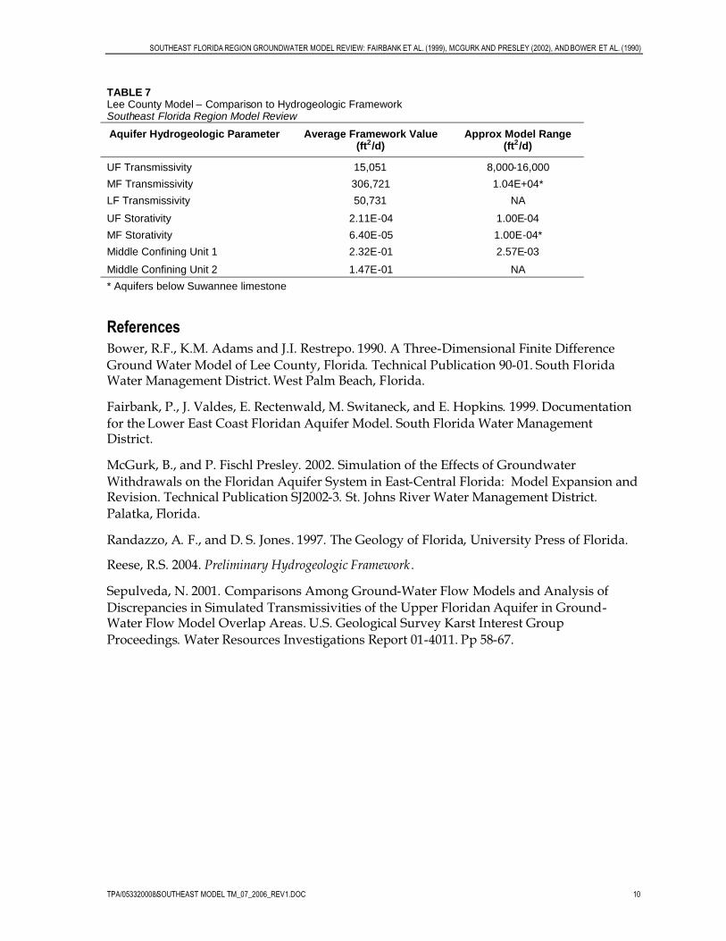
SOUTHEAST FLORIDA REGION GROUNDWATER MODEL REVIEW: FAIRBANK ET AL. (1999), MCGURK AND PRESLEY (2002), AND BOWER ET AL. (1990)
TPA/053320008/SOUTHEAST MODEL TM_07_2006_REV1.DOC 10
TABLE 7Lee County Model – Comparison to Hydrogeologic FrameworkSoutheast Florida Region Model Review
Aquifer Hydrogeologic Parameter Average Framework Value(ft2/d)
Approx Model Range(ft2/d)
UF Transmissivity 15,051 8,000-16,000
MF Transmissivity 306,721 1.04E+04*
LF Transmissivity 50,731 NA
UF Storativity 2.11E-04 1.00E-04
MF Storativity 6.40E-05 1.00E-04*
Middle Confining Unit 1 2.32E-01 2.57E-03
Middle Confining Unit 2 1.47E-01 NA
* Aquifers below Suwannee limestone
References
Bower, R.F., K.M. Adams and J.I. Restrepo. 1990. A Three-Dimensional Finite Difference
Ground Water Model of Lee County, Florida. Technical Publication 90-01. South FloridaWater Management District.West Palm Beach, Florida.
Fairbank, P., J. Valdes, E. Rectenwald, M. Switaneck, and E. Hopkins. 1999. Documentation
for the Lower East Coast Floridan Aquifer Model. South Florida Water ManagementDistrict.
McGurk, B., and P. Fischl Presley. 2002. Simulation of the Effects of Groundwater
Withdrawals on the Floridan Aquifer System in East-Central Florida: Model Expansion andRevision. Technical Publication SJ2002-3. St. Johns River Water Management District.
Palatka, Florida.
Randazzo, A. F., and D. S. Jones. 1997. The Geology of Florida, University Press of Florida.
Reese, R.S. 2004. Preliminary Hydrogeologic Framework .
Sepulveda, N. 2001. Comparisons Among Ground-Water Flow Models and Analysis of
Discrepancies in Simulated Transmissivities of the Upper Floridan Aquifer in Ground-Water Flow Model Overlap Areas. U.S. Geological Survey Karst Interest Group
Proceedings. Water Resources Investigations Report 01-4011. Pp 58-67.

FIGURE

Franklin
Gadsden
Leon
Wakulla
Alachua
Baker
Bradfo
rd
Bre
vard
Broward
Charlotte
Citrus
Clay
Collier
Col
umbi
a
Dade
De Soto
Dixie
Duval
Flagler
Gilc
hrist
Glades
Hamilton
Hardee
Hendry
Hernando
Highlands
Hillsborough
Indian
River
Jeffe
rson
Lafayette
Lake
Lee
Levy
Madison
Manatee
Marion
Martin
Monroe
Okeechobee
Palm Beach
Pasco
Pin
ella
s
Polk
Putnam
St. Jo
hns
St. Lucie
Sarasota
Seminole
Sum
ter
Suwannee
TaylorUnion
Volusia
Liberty
Orange
Osceola
Nassau
W102005002TPA_334350.TW.03
North
FIGURE 1
Reviewed Model Boundaries
USACE - Subtask 3 Model Development
19
22
29
Bower, Adams and Restrepo (SFWMD 1990)
Fairbank and Others (SFWMD 1999) - LECFA Model
McGurk and Presley (SJRWMD 2002)
ModelNumber
Authors(Organization and Year)
0 3015
Approximate Scale in Miles

TPA/053320008/SOUTHEAST MODEL TM_07_2006_REV1.DOC 11
Appendix A
Selected Figures from Documentation of Lower East Coast Florida model
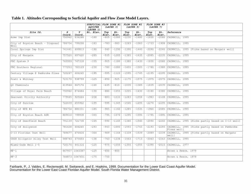
Table 1. Altitudes Corresponding to Surficial Aquifer and Flow Zone Model Layers.
35
SURFICIALAQUIFER(LAYER 1)
FLOW ZONE #1(LAYER 3)
FLOW ZONE #2(LAYER 5)
FLOW ZONE #3(LAYER 7)
Site Id. XCoord.
YCoord.
Bt. Elev. TopElev.
Bt.Elev.
TopElev.
Bt.Elev.
TopElev.
Bt.Elev.
Reference
Acme Imp Dist 750942 834288 -180 -805 -1080 -1230 -1480 -1830 -2080 CH2MHILL, 1995
City of Boynton Beach - DisposalWell
786754 799208 -183 -783 -983 -1283 -1583 -1733 -1908 CH2MHILL, 1995
Coral Springs Imp Dist 741441 699813 -190 -940 -1290 -1390 -1440 -2090 -2240 CH2MHILL, 1995 [Picks based on Margate well]
City of Margate 757520 697620 -285 -935 -1285 -1385 -1435 -2085 -2235 CH2MHILL, 1995
PBC System 9 765559 747318 -155 -905 -1180 -1380 -1430 -1830 -2080 CH2MHILL, 1995
PBC Southern Regional 777253 783129 -230 -780 -1080 -1455 -1505 -1780 -1980 CH2MHILL, 1995
Century Village @ Pembroke Pines 720247 606265 -195 -995 -1120 -1595 -1745 -2195 -2295 CH2MHILL, 1995
Pratt & Whitney 723170 938799 -125 -850 -925 -1175 -1575 -1975 -2075 CH2MHILL, 1995
QO Chemicals 613544 867176 -160 -635 -810 -1035 -1385 -1835 -2035 CH2MHILL, 1995
Village of Royal Palm Beach 750942 874484 -130 -880 -1055 -1205 -1430 -2180 -2380 CH2MHILL, 1995
Seacoast Utility Authority 779445 925644 -258 -883 -1033 -1283 -1558 -1983 -2108 CH2MHILL, 1995
City of Sunrise 722439 655962 -195 -995 -1345 -1545 -1695 -2270 -2295 CH2MHILL, 1995
City of WPB #6 786754 880331 -185 -985 -1160 -1285 -1535 -1960 -2085 CH2MHILL, 1995
City of Boynton Beach ASR 809410 799938 -345 -795 -1070 -1295 -1595 -1795 -1895 CH2MHILL, 1995
City of Deerfield Beach 791139 721738 -165 -990 -1165 -1340 -1540 -2090 -2240 CH2MHILL, 1995 [Picks partly based on C-13 well]
City of Hollywood 781638 606265 -293 -943 -1093 -1593 -1743 -2193 -2293 CH2MHILL, 1995 [Picks partly based on PembrokePines well]
C-13 Floridan Test Well 789677 676426 -364 -989 -1164 -1339 -1539 -2089 -2239 CH2MHILL, 1995 [Picks partly based on Margatewell]
USGS Alligator Alley Test Well 548743 675603 -138 -763 -1238 -1563 -1713 -2063 -2263 CH2MHILL, 1995
Miami-Dade Well I-5 720170 441316 -125 -975 -1055 -1355 -1555 -2395 -2515 CH2MHILL, 1977
MF-1 667937 1043387 -125 -650 -800 Brown & Reece, 1979
MF-3 766873 1047651 -175 -750 Brown & Reece, 1979
Fairbank, P., J. Valdes, E. Rectenwald, M. Switaneck, and E. Hopkins, 1999. Documentation for the Lower East Coast Aquifer Model.Documentation for the Lower East Coast Floridan Aquifer Model. South Florida Water Management District.
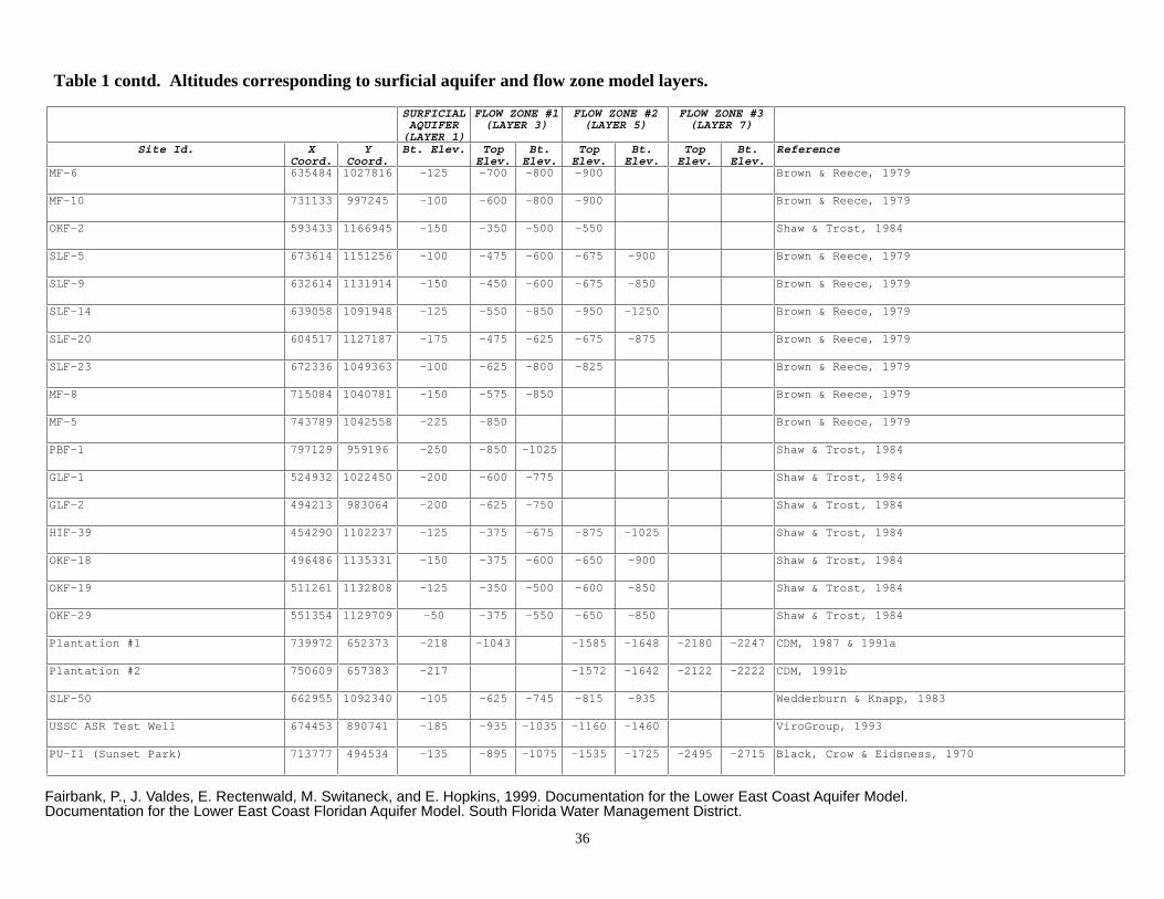
Table 1 contd. Altitudes corresponding to surficial aquifer and flow zone model layers.
36
SURFICIALAQUIFER(LAYER 1)
FLOW ZONE #1(LAYER 3)
FLOW ZONE #2(LAYER 5)
FLOW ZONE #3(LAYER 7)
Site Id. XCoord.
YCoord.
Bt. Elev. TopElev.
Bt.Elev.
TopElev.
Bt.Elev.
TopElev.
Bt.Elev.
Reference
MF-6 635484 1027816 -125 -700 -800 -900 Brown & Reece, 1979
MF-10 731133 997245 -100 -600 -800 -900 Brown & Reece, 1979
OKF-2 593433 1166945 -150 -350 -500 -550 Shaw & Trost, 1984
SLF-5 673614 1151256 -100 -475 -600 -675 -900 Brown & Reece, 1979
SLF-9 632614 1131914 -150 -450 -600 -675 -850 Brown & Reece, 1979
SLF-14 639058 1091948 -125 -550 -850 -950 -1250 Brown & Reece, 1979
SLF-20 604517 1127187 -175 -475 -625 -675 -875 Brown & Reece, 1979
SLF-23 672336 1049363 -100 -625 -800 -825 Brown & Reece, 1979
MF-8 715084 1040781 -150 -575 -850 Brown & Reece, 1979
MF-5 743789 1042558 -225 -850 Brown & Reece, 1979
PBF-1 797129 959196 -250 -850 -1025 Shaw & Trost, 1984
GLF-1 524932 1022450 -200 -600 -775 Shaw & Trost, 1984
GLF-2 494213 983064 -200 -625 -750 Shaw & Trost, 1984
HIF-39 454290 1102237 -125 -375 -675 -875 -1025 Shaw & Trost, 1984
OKF-18 496486 1135331 -150 -375 -600 -650 -900 Shaw & Trost, 1984
OKF-19 511261 1132808 -125 -350 -500 -600 -850 Shaw & Trost, 1984
OKF-29 551354 1129709 -50 -375 -550 -650 -850 Shaw & Trost, 1984
Plantation #1 739972 652373 -218 -1043 -1585 -1648 -2180 -2247 CDM, 1987 & 1991a
Plantation #2 750609 657383 -217 -1572 -1642 -2122 -2222 CDM, 1991b
SLF-50 662955 1092340 -105 -625 -745 -815 -935 Wedderburn & Knapp, 1983
USSC ASR Test Well 674453 890741 -185 -935 -1035 -1160 -1460 ViroGroup, 1993
PU-I1 (Sunset Park) 713777 494534 -135 -895 -1075 -1535 -1725 -2495 -2715 Black, Crow & Eidsness, 1970
Fairbank, P., J. Valdes, E. Rectenwald, M. Switaneck, and E. Hopkins, 1999. Documentation for the Lower East Coast Aquifer Model.Documentation for the Lower East Coast Floridan Aquifer Model. South Florida Water Management District.

Table 1 contd. Altitudes corresponding to surficial aquifer and flow zone model layers.
37
SURFICIALAQUIFER(LAYER 1)
FLOW ZONE #1(LAYER 3)
FLOW ZONE #2(LAYER 5)
FLOW ZONE #3(LAYER 7)
Site Id. XCoord.
YCoord.
Bt. Elev. TopElev.
Bt.Elev.
TopElev.
Bt.Elev.
TopElev.
Bt.Elev.
Reference
PU-I2 (Kendale Lakes) 692558 493627 -115 -1055 -1095 -1505 -1735 -2495 -2705 Black, Crow & Eidsness, 1972
G-3061 (Hialeah ASR well) 734185 543807 -1019 -1031 Reese, 1994
NP-100 631054 381242 -965 -1005 -1165 -1328 Meyer, 1971
S-524 636935 465655 -1132 -1192 Meyer, 1971
G-1273 695665 287597 -800 -890 Meyer, 1971
W-2912 500053 882046 -1185 -1295 -1605 -1645 -2045 -2085 Puri & Winston, 1974
W-4661 573250 735652 -905 -935 -1215 -1235 Puri & Winston, 1974
W-445 535188 483855 -910 -930 -1440 -1470 -1920 -2050 Puri & Winston, 1974
Jupiter RO facility (multi-wellcomposite)
778291 944693 -1035 -1315 -1645 -1815 ViroGroup, 1994
Stuart Injection Well IW-2 748598 1038851 -975 -1055 Montgomery Watson, 1997
City of Miramar IW-1 724512 594136 -183 -1063 -1133 -1632 -1731 -1913 -1998 Montgomery Watson, 1996
City of WPB ASR 804703 864431 -355 -960 -1185 CH2MHill, 1998b
City of Sunrise ASR 742533 667332 -182 -1102 -1262 Montgomery Watson, 1998
City of Delray Beach ASR 741876 782028 -1006 -1190 CH2MHill, 1998a
West Wellfield ASR 672876 496977 -166 -831 -1241 CH2MHill, 1997b
PBC System 3 MultipurposeFloridan Well
782494 782181 -320 -1040 Kimley-Horn & Assoc., 1998
BCOES ASR facility 792605 713184 -362 -977 -1182 CH2MHill, 1997a
Indiantown Cogeneration Project(IPW-1)
657324 985586 -133 -675 -695 -745 -775 -1435 -1475 Bechtel Corp., 1991 & 1994
SFWMD Okeechobee ASR Demo. Proj. 570202 1053544 -125 -1283 -1605 CH2MHill, 1989a
DBF R0-1/BF-6 786910 720819 -412 -947 -1115 Lukasiewicz, SFWMD (unpublished data)
BF-3/BF-1 769399 669411 -395 -995 -1195 -1495 -1595 -2095 -2145 Lukasiewicz, SFWMD (unpublished data)
Fairbank, P., J. Valdes, E. Rectenwald, M. Switaneck, and E. Hopkins, 1999. Documentation for the Lower East Coast Aquifer Model.Documentation for the Lower East Coast Floridan Aquifer Model. South Florida Water Management District.
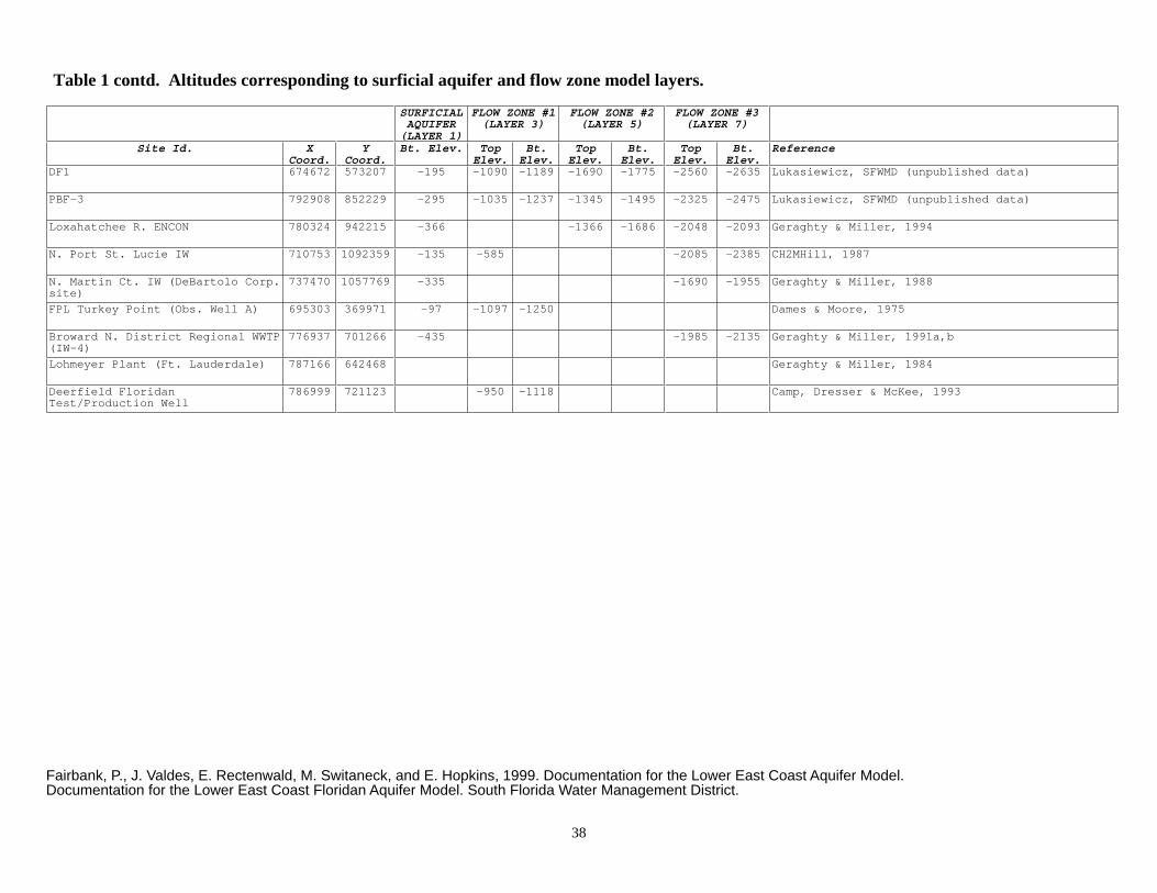
Table 1 contd. Altitudes corresponding to surficial aquifer and flow zone model layers.
38
SURFICIALAQUIFER(LAYER 1)
FLOW ZONE #1(LAYER 3)
FLOW ZONE #2(LAYER 5)
FLOW ZONE #3(LAYER 7)
Site Id. XCoord.
YCoord.
Bt. Elev. TopElev.
Bt.Elev.
TopElev.
Bt.Elev.
TopElev.
Bt.Elev.
Reference
DF1 674672 573207 -195 -1090 -1189 -1690 -1775 -2560 -2635 Lukasiewicz, SFWMD (unpublished data)
PBF-3 792908 852229 -295 -1035 -1237 -1345 -1495 -2325 -2475 Lukasiewicz, SFWMD (unpublished data)
Loxahatchee R. ENCON 780324 942215 -366 -1366 -1686 -2048 -2093 Geraghty & Miller, 1994
N. Port St. Lucie IW 710753 1092359 -135 -585 -2085 -2385 CH2MHill, 1987
N. Martin Ct. IW (DeBartolo Corp.site)
737470 1057769 -335 -1690 -1955 Geraghty & Miller, 1988
FPL Turkey Point (Obs. Well A) 695303 369971 -97 -1097 -1250 Dames & Moore, 1975
Broward N. District Regional WWTP(IW-4)
776937 701266 -435 -1985 -2135 Geraghty & Miller, 1991a,b
Lohmeyer Plant (Ft. Lauderdale) 787166 642468 Geraghty & Miller, 1984
Deerfield FloridanTest/Production Well
786999 721123 -950 -1118 Camp, Dresser & McKee, 1993
Fairbank, P., J. Valdes, E. Rectenwald, M. Switaneck, and E. Hopkins, 1999. Documentation for the Lower East Coast Aquifer Model.Documentation for the Lower East Coast Floridan Aquifer Model. South Florida Water Management District.
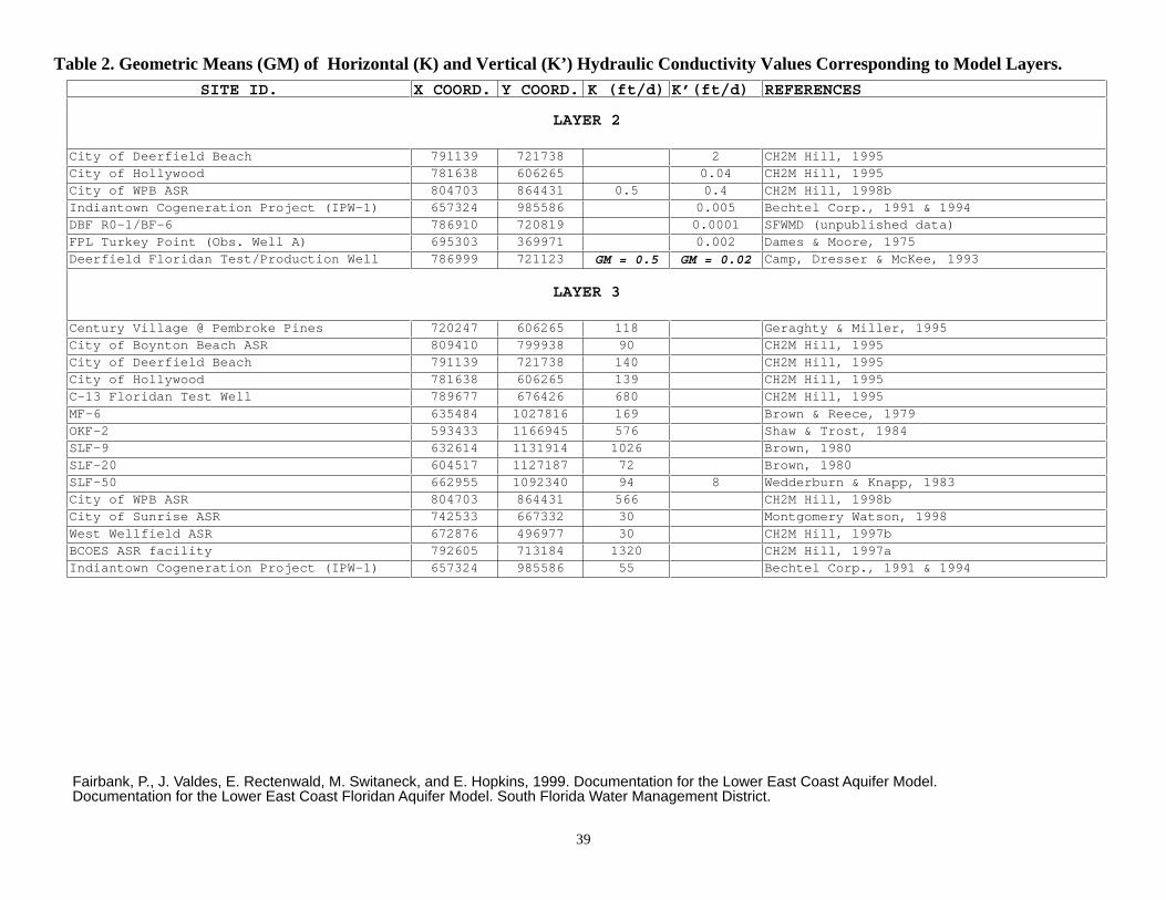
Table 2. Geometric Means (GM) of Horizontal (K) and Vertical (K’) Hydraulic Conductivity Values Corresponding to Model Layers.
39
SITE ID. X COORD. Y COORD. K (ft/d) K’(ft/d) REFERENCES
LAYER 2
City of Deerfield Beach 791139 721738 2 CH2M Hill, 1995City of Hollywood 781638 606265 0.04 CH2M Hill, 1995City of WPB ASR 804703 864431 0.5 0.4 CH2M Hill, 1998bIndiantown Cogeneration Project (IPW-1) 657324 985586 0.005 Bechtel Corp., 1991 & 1994DBF R0-1/BF-6 786910 720819 0.0001 SFWMD (unpublished data)FPL Turkey Point (Obs. Well A) 695303 369971 0.002 Dames & Moore, 1975Deerfield Floridan Test/Production Well 786999 721123 GM = 0.5 GM = 0.02 Camp, Dresser & McKee, 1993
LAYER 3
Century Village @ Pembroke Pines 720247 606265 118 Geraghty & Miller, 1995City of Boynton Beach ASR 809410 799938 90 CH2M Hill, 1995City of Deerfield Beach 791139 721738 140 CH2M Hill, 1995City of Hollywood 781638 606265 139 CH2M Hill, 1995C-13 Floridan Test Well 789677 676426 680 CH2M Hill, 1995MF-6 635484 1027816 169 Brown & Reece, 1979OKF-2 593433 1166945 576 Shaw & Trost, 1984SLF-9 632614 1131914 1026 Brown, 1980SLF-20 604517 1127187 72 Brown, 1980SLF-50 662955 1092340 94 8 Wedderburn & Knapp, 1983City of WPB ASR 804703 864431 566 CH2M Hill, 1998bCity of Sunrise ASR 742533 667332 30 Montgomery Watson, 1998West Wellfield ASR 672876 496977 30 CH2M Hill, 1997bBCOES ASR facility 792605 713184 1320 CH2M Hill, 1997aIndiantown Cogeneration Project (IPW-1) 657324 985586 55 Bechtel Corp., 1991 & 1994
Fairbank, P., J. Valdes, E. Rectenwald, M. Switaneck, and E. Hopkins, 1999. Documentation for the Lower East Coast Aquifer Model.Documentation for the Lower East Coast Floridan Aquifer Model. South Florida Water Management District.
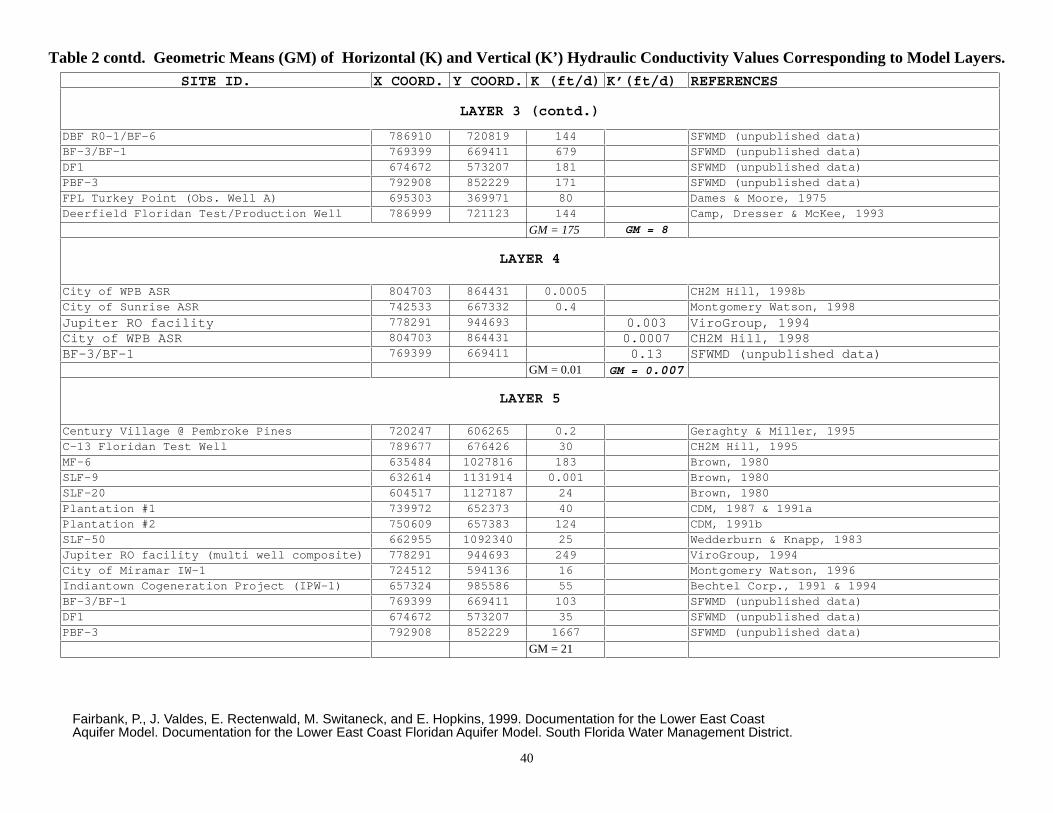
Table 2 contd. Geometric Means (GM) of Horizontal (K) and Vertical (K’) Hydraulic Conductivity Values Corresponding to Model Layers.
40
SITE ID. X COORD. Y COORD. K (ft/d) K’(ft/d) REFERENCES
LAYER 3 (contd.)
DBF R0-1/BF-6 786910 720819 144 SFWMD (unpublished data)BF-3/BF-1 769399 669411 679 SFWMD (unpublished data)DF1 674672 573207 181 SFWMD (unpublished data)PBF-3 792908 852229 171 SFWMD (unpublished data)FPL Turkey Point (Obs. Well A) 695303 369971 80 Dames & Moore, 1975Deerfield Floridan Test/Production Well 786999 721123 144 Camp, Dresser & McKee, 1993
GM = 175 GM = 8
LAYER 4
City of WPB ASR 804703 864431 0.0005 CH2M Hill, 1998bCity of Sunrise ASR 742533 667332 0.4 Montgomery Watson, 1998
Jupiter RO facility 778291 944693 0.003 ViroGroup, 1994City of WPB ASR 804703 864431 0.0007 CH2M Hill, 1998BF-3/BF-1 769399 669411 0.13 SFWMD (unpublished data)
GM = 0.01 GM = 0.007
LAYER 5
Century Village @ Pembroke Pines 720247 606265 0.2 Geraghty & Miller, 1995C-13 Floridan Test Well 789677 676426 30 CH2M Hill, 1995MF-6 635484 1027816 183 Brown, 1980SLF-9 632614 1131914 0.001 Brown, 1980SLF-20 604517 1127187 24 Brown, 1980Plantation #1 739972 652373 40 CDM, 1987 & 1991aPlantation #2 750609 657383 124 CDM, 1991bSLF-50 662955 1092340 25 Wedderburn & Knapp, 1983Jupiter RO facility (multi well composite) 778291 944693 249 ViroGroup, 1994City of Miramar IW-1 724512 594136 16 Montgomery Watson, 1996Indiantown Cogeneration Project (IPW-1) 657324 985586 55 Bechtel Corp., 1991 & 1994BF-3/BF-1 769399 669411 103 SFWMD (unpublished data)DF1 674672 573207 35 SFWMD (unpublished data)PBF-3 792908 852229 1667 SFWMD (unpublished data)
GM = 21
Fairbank, P., J. Valdes, E. Rectenwald, M. Switaneck, and E. Hopkins, 1999. Documentation for the Lower East Coast Aquifer Model. Documentation for the Lower East Coast Floridan Aquifer Model. South Florida Water Management District.

Table 2 contd. Geometric Means (GM) of Horizontal (K) and Vertical (K’) Hydraulic Conductivity Values Corresponding to Model Layers.
41
SITE ID. X COORD. Y COORD. K (ft/d) K’(ft/d) REFERENCES
LAYER 6
Acme Imp Dist 750942 834288 0.4 CH2M Hill, 1995Coral Springs Imp Dist 741441 699813 0.04 0.16 Geraghty and Miller, 1986C-13 Floridan Test Well 789677 676426 0.4 CH2M Hill, 1995Miami-Dade Well I-5 720170 441316 3 CH2M Hill, 1977; Hydrologic Assoc., 1994Plantation #1 739972 652373 17 0.1 CDM, 1987 & 1991aPlantation #2 750609 657383 37 3 CDM, 1991bCity of Miramar IW-1 724512 594136 21 0.09 Montgomery Watson, 1996BF-3/BF-1 769399 669411 5 SFWMD (unpublished data)Indiantown Cogeneration Project (IPW-1) 657324 985586 0.96 Bechtel Corp., 1991 & 1994SFWMD Okeechobee ASR Demo. Proj. 570202 1053544 0.4 CH2M Hill, 1989Broward N. District Regional WWTP (IW-4) 776937 701266 0.4 Geraghty & Miller, 1991a,b
GM = 2 GM = 0.35
LAYER 7
Acme Imp Dist 750942 834288 14 CH2M Hill, 1995Coral Springs Imp Dist 741441 699813 0.03 0.22 Geraghty & Miller, 1986PBC Southern Regional 777253 783129 116 CH2M Hill, 1995C-13 Floridan Test Well 789677 676426 210 CH2M Hill, 1995Plantation #2 750609 657383 94 CDM, 1991bCity of Miramar IW-1 724512 594136 20 Montgomery Watson, 1996Indiantown Cogeneration Project (IPW-1) 657324 985586 2055 Bechtel Corp., 1991 & 1994SFWMD Okeechobee ASR Demo. Proj. 570202 1053544 1470 CH2M Hill, 1989aBF-3/BF-1 769399 669411 205 SFWMD (unpublished data)DF1 674672 573207 40 SFWMD (unpublished data)PBF-3 792908 852229 7 SFWMD (unpublished data)Loxahatchee R. ENCON 780324 942215 1313 Geraghty & Miller, 1994N. Martin Ct. IW (DeBartolo Corp. site) 737470 1057769 32 Geraghty & Miller, 1988
GM = 60 GM = 0.22
LAYER 8
Acme Imp Dist 750942 834288 7 CH2M HIll, 1995Coral Springs Imp Dist 741441 699813 0.05 CH2M Hill, 1995; Geraghty & Miller, 1986Century Village @ Pembroke Pines 720247 606265 2 Geraghty & Miller, 1995Village of Royal Palm Beach 750942 874484 0.005 0.001 CH2MHILL, 1995Seacoast Utility Authority 779445 925644 0.003 0.002 CH2M Hill, 1989bPlantation #1 739972 652373 5 0.07 CDM, 1987 & 1991a
Fairbank, P., J. Valdes, E. Rectenwald, M. Switaneck, and E. Hopkins, 1999. Documentation for the Lower East Coast Aquifer Model.Documentation for the Lower East Coast Floridan Aquifer Model.South Florida Water Management District.

Table 2 contd. Geometric Means (GM) of Horizontal (K) and Vertical (K’) Hydraulic Conductivity Values Corresponding to Model Layers.
42
SITE ID. X COORD. Y COORD. K (ft/d) K’(ft/d) REFERENCES
LAYER 8 (contd.)
Plantation #2 750609 657383 4 0.3 CDM, 1991bCity of Miramar IW-1 724512 594136 0.9 0.0009 Montgomery Watson, 1996N. Port St. Lucie IW 710753 1092359 0.00013 0.000051 CH2MHill, 1987N. Martin Ct. IW (DeBartolo Corp. site) 737470 1057769 4 0.00041 Geraghty & Miller, 1988Broward N. District Regional WWTP (IW-4) 776937 701266 1 Geraghty & Miller, 1991a,bCoral Springs Imp Dist 741441 699813 0.004 Geraghty & Miller, 1986
PBC System 9 765559 747318 0.002 CH2M Hill, 1986PBC System 3 Multipurpose Floridan Well 782494 782181 0.02 Kimley-Horn, 1998; Geraghty & Miller, 1987Lohmeyer Plant (Ft. Lauderdale) 787166 642468 0.1 Geraghty & Miller, 1984
GM = 0.2 GM = 0.004
LAYER 9
Coral Springs Imp Dist 741441 699813 1000 Geraghty & Miller, 1986Century Village @ Pembroke Pines 720247 606265 733 Geraghty & Miller, 1995Miami-Dade Well I-5 720170 441316 58565 Singh et al., 1983Plantation #2 750609 657383 133 3 CDM, 1991bPBC System 3 Multipurpose Floridan Well 782494 782181 607 Kimley-Horn, 1998; Geraghty & Miller, 1987N. Martin Ct. IW (DeBartolo Corp. site) 737470 1057769 804 Geraghty & Miller, 1988Lohmeyer Plant (Ft. Lauderdale) 787166 642468 19647 Geraghty & Miller, 1984
GM = 1771 GM = 3
Fairbank, P., J. Valdes, E. Rectenwald, M. Switaneck, and E. Hopkins, 1999. Documentation for the Lower East Coast Aquifer Model.Documentation for the Lower East Coast Floridan Aquifer Model. South Florida Water Management District.
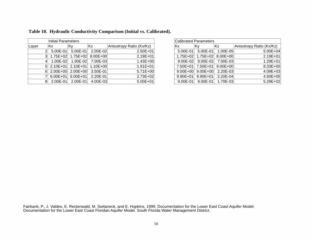
Table 10. Hydraulic Conductivity Comparison (Initial vs. Calibrated).
50
Initial Parameters Calibrated ParametersLayer Kx Ky Kz Anisotropy Ratio (Kx/Kz) Kx Ky Kz Anisotropy Ratio (Kx/Kz)
2 5.00E-01 5.00E-01 2.00E-02 2.50E+01 5.00E-01 5.00E-01 1.00E-05 5.00E+043 1.75E+02 1.75E+02 8.00E+00 2.19E+01 1.75E+02 1.75E+02 8.00E+00 2.19E+014 1.00E-02 1.00E-02 7.00E-03 1.43E+00 9.00E-02 9.00E-02 7.00E-03 1.29E+015 2.10E+01 2.10E+01 1.10E+00 1.91E+01 7.50E+01 7.50E+01 9.00E+00 8.33E+006 2.00E+00 2.00E+00 3.50E-01 5.71E+00 9.00E+00 9.00E+00 2.20E-03 4.09E+037 6.00E+01 6.00E+01 2.20E-01 2.73E+02 9.90E+01 9.90E+01 2.20E-04 4.50E+058 2.00E-01 2.00E-01 4.00E-03 5.00E+01 9.00E-01 9.00E-01 1.70E-03 5.29E+02
Fairbank, P., J. Valdes, E. Rectenwald, M. Switaneck, and E. Hopkins, 1999. Documentation for the Lower East Coast Aquifer Model.Documentation for the Lower East Coast Floridan Aquifer Model. South Florida Water Management District.

17
Figure 1. Model Grid Domain.
Fairbank, P., J. Valdes, E. Rectenwald, M. Switaneck, and E. Hopkins, 1999. Documentation for the Lower East Coast Aquifer Model. Documentation for the Lower East Coast Floridan Aquifer Model. South Florida Water Management District.
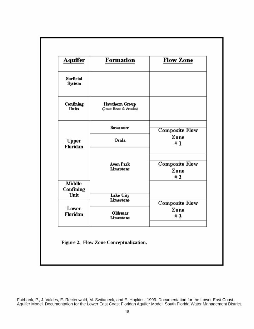
18
Figure 2. Flow Zone Conceptualization.
Fairbank, P., J. Valdes, E. Rectenwald, M. Switaneck, and E. Hopkins, 1999. Documentation for the Lower East Coast Aquifer Model. Documentation for the Lower East Coast Floridan Aquifer Model. South Florida Water Management District.
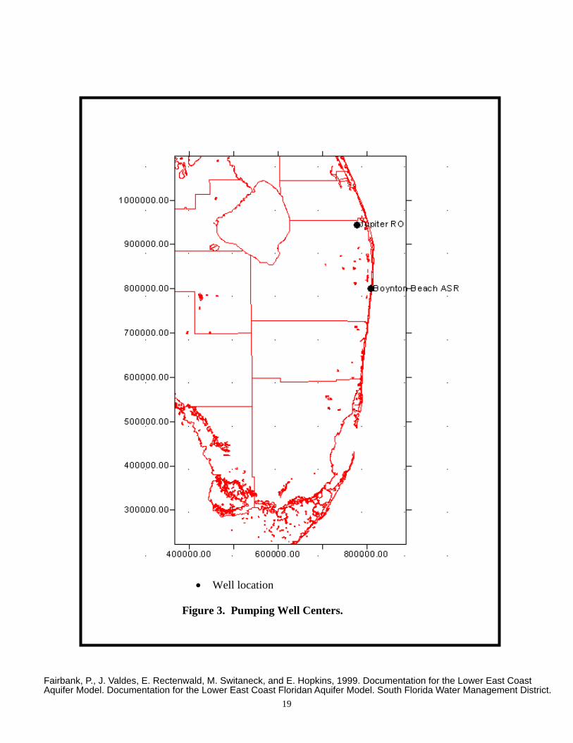
19
Figure 3. Pumping Well Centers.
• Well location
Fairbank, P., J. Valdes, E. Rectenwald, M. Switaneck, and E. Hopkins, 1999. Documentation for the Lower East Coast Aquifer Model. Documentation for the Lower East Coast Floridan Aquifer Model. South Florida Water Management District.

20
400000.00 600000.00 800000.00
Layer 1 - Surface Elevation - 2.50’
300000.00
400000.00
500000.00
600000.00
700000.00
800000.00
900000.00
1000000.00
Figure 4. Initial Head Distribution – Layer 1.
Active cell boundary
Fairbank, P., J. Valdes, E. Rectenwald, M. Switaneck, and E. Hopkins, 1999. Documentation for the Lower East Coast Aquifer Model. Documentation for the Lower East Coast Floridan Aquifer Model. South Florida Water Management District.
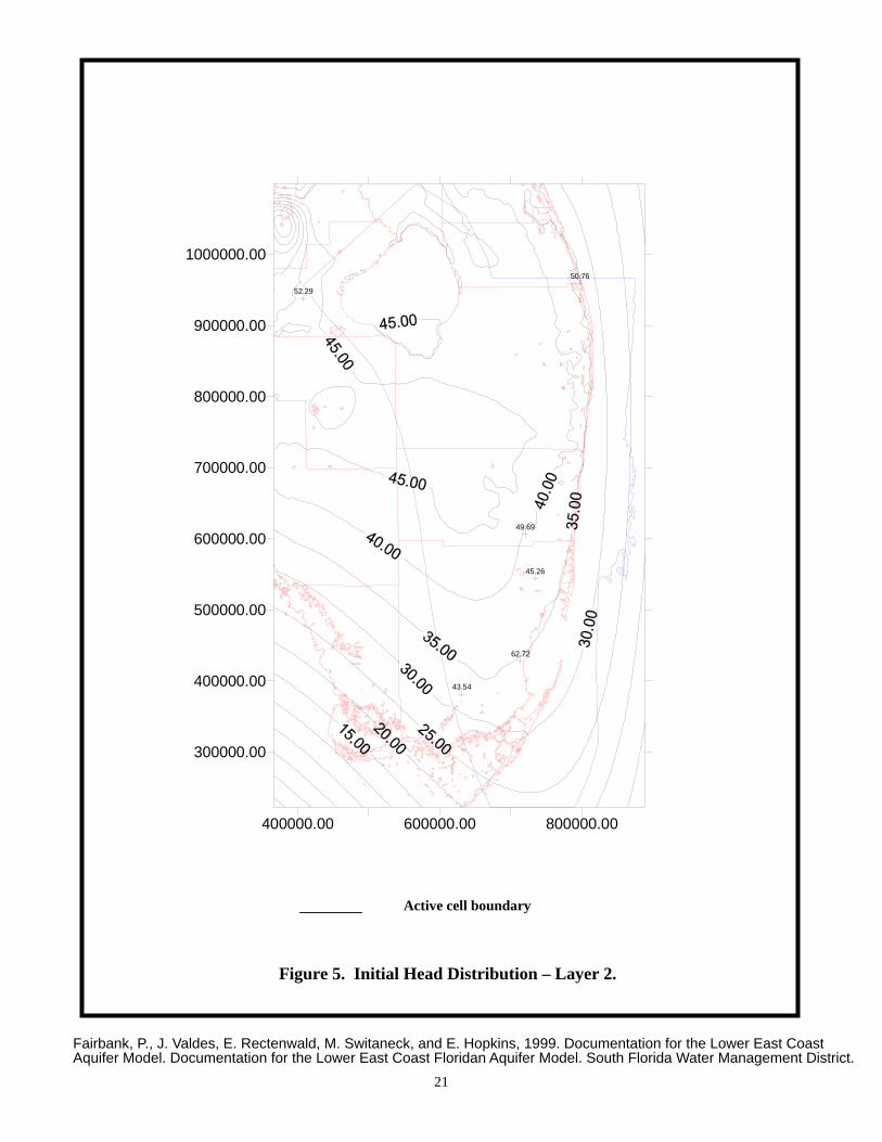
21
400000.00 600000.00 800000.00
Layer 2(1/4 layer1 + 3/4 layer 3)
300000.00
400000.00
500000.00
600000.00
700000.00
800000.00
900000.00
1000000.0050.76
62.72
49.69
45.26
43.54
52.29
Figure 5. Initial Head Distribution – Layer 2.
Active cell boundary
Fairbank, P., J. Valdes, E. Rectenwald, M. Switaneck, and E. Hopkins, 1999. Documentation for the Lower East Coast Aquifer Model. Documentation for the Lower East Coast Floridan Aquifer Model. South Florida Water Management District.
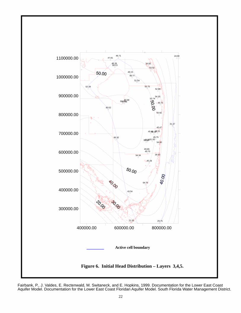
22
37.99
50.92
46.3145.65
54.80
49.32
39.93
43.70
64.70
54.35
49.69
61.05
34.00
60.6852.74
53.5043.35
52.88
52.52
50.70
59.18
45.75
45.47
60.32
54.34
45.26
43.54
60.52
49.75
52.29
51.54
48.77
48.15
50.1346.26
47.8146.71
31.37
29.7522.35
24.00
400000.00 600000.00 800000.00
Layer 3,4 & 5(Cubic Surface - 3rd Order)
300000.00
400000.00
500000.00
600000.00
700000.00
800000.00
900000.00
1000000.00
1100000.00
Figure 6. Initial Head Distribution – Layers 3,4,5.
Active cell boundary
Fairbank, P., J. Valdes, E. Rectenwald, M. Switaneck, and E. Hopkins, 1999. Documentation for the Lower East Coast Aquifer Model. Documentation for the Lower East Coast Floridan Aquifer Model. South Florida Water Management District.

23
50.1054.24
51.00
77.08
53.44
49.07
59.16
90.60
65.90
34.58
400000.00 600000.00 800000.00
Layer 6(3/4 of Lay. 3,4&5 - 3rd Order & 1/4 of Lay. 7 - 1st Order)
300000.00
400000.00
500000.00
600000.00
700000.00
800000.00
900000.00
1000000.00
1100000.00
Figure 7. Initial Head Distribution – Layer 6.
Active cell boundary
Fairbank, P., J. Valdes, E. Rectenwald, M. Switaneck, and E. Hopkins, 1999. Documentation for the Lower East Coast Aquifer Model. Documentation for the Lower East Coast Floridan Aquifer Model. South Florida Water Management District.

24
Figure 8. Initial Head Distribution – Layer 7.
Active cell boundary
77.15
71.32
78.73
70.10
62.87
28.76
400000.00 600000.00 800000.00
Layer 7 - 1st Order
300000.00
400000.00
500000.00
600000.00
700000.00
800000.00
900000.00
1000000.00
Fairbank, P., J. Valdes, E. Rectenwald, M. Switaneck, and E. Hopkins, 1999. Documentation for the Lower East Coast Aquifer Model. Documentation for the Lower East Coast Floridan Aquifer Model. South Florida Water Management District.

25
67.60
400000.00 600000.00 800000.00
Layer 8 - 1st Order of Layer 7 + 5.00’
300000.00
400000.00
500000.00
600000.00
700000.00
800000.00
900000.00
1000000.00
Figure 9. Initial Head Distribution – Layer 8.
Active cell boundary
Fairbank, P., J. Valdes, E. Rectenwald, M. Switaneck, and E. Hopkins, 1999. Documentation for the Lower East Coast Aquifer Model. Documentation for the Lower East Coast Floridan Aquifer Model. South Florida Water Management District.
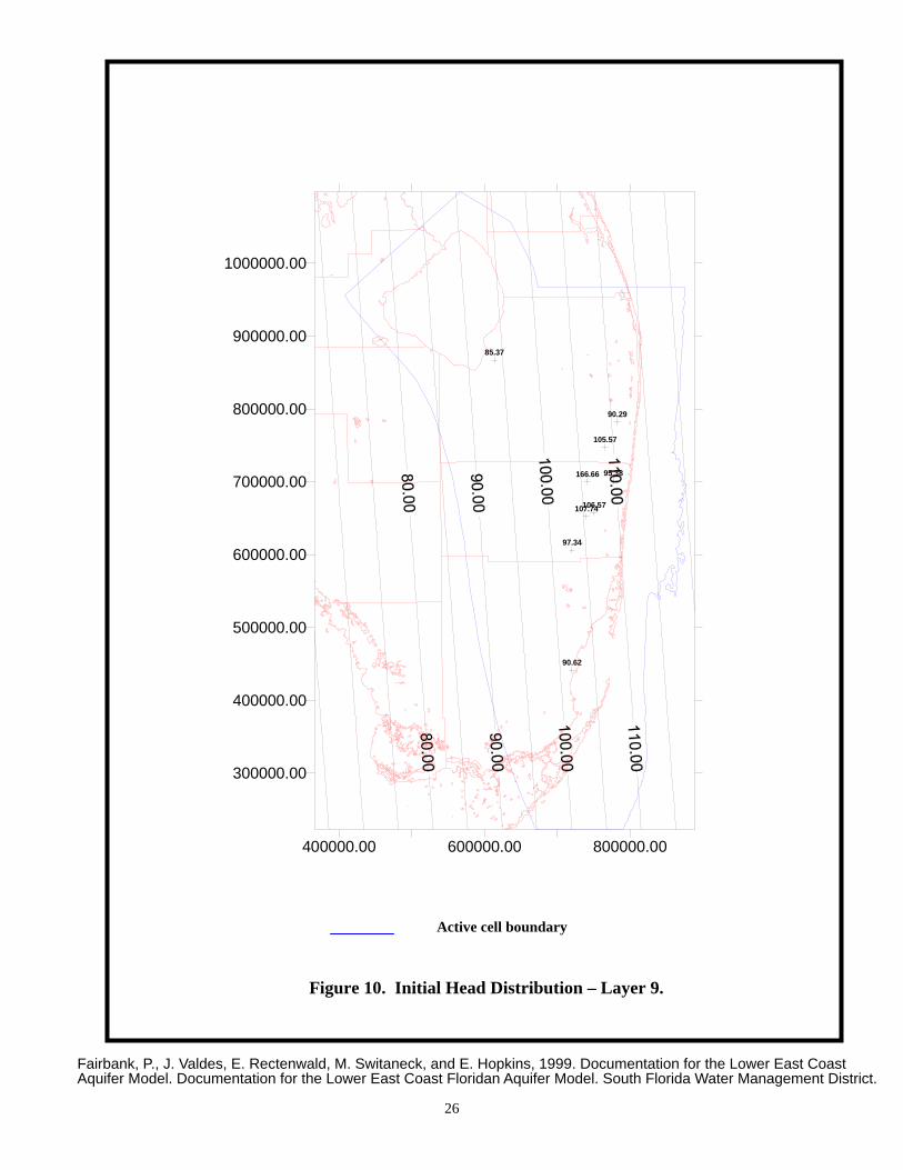
26
166.66
105.57
97.34
90.62
107.74106.57
90.29
95.38
85.37
400000.00 600000.00 800000.00
Layer 9 - 1st Order
300000.00
400000.00
500000.00
600000.00
700000.00
800000.00
900000.00
1000000.00
Figure 10. Initial Head Distribution – Layer 9.
Active cell boundary
Fairbank, P., J. Valdes, E. Rectenwald, M. Switaneck, and E. Hopkins, 1999. Documentation for the Lower East Coast Aquifer Model. Documentation for the Lower East Coast Floridan Aquifer Model. South Florida Water Management District.
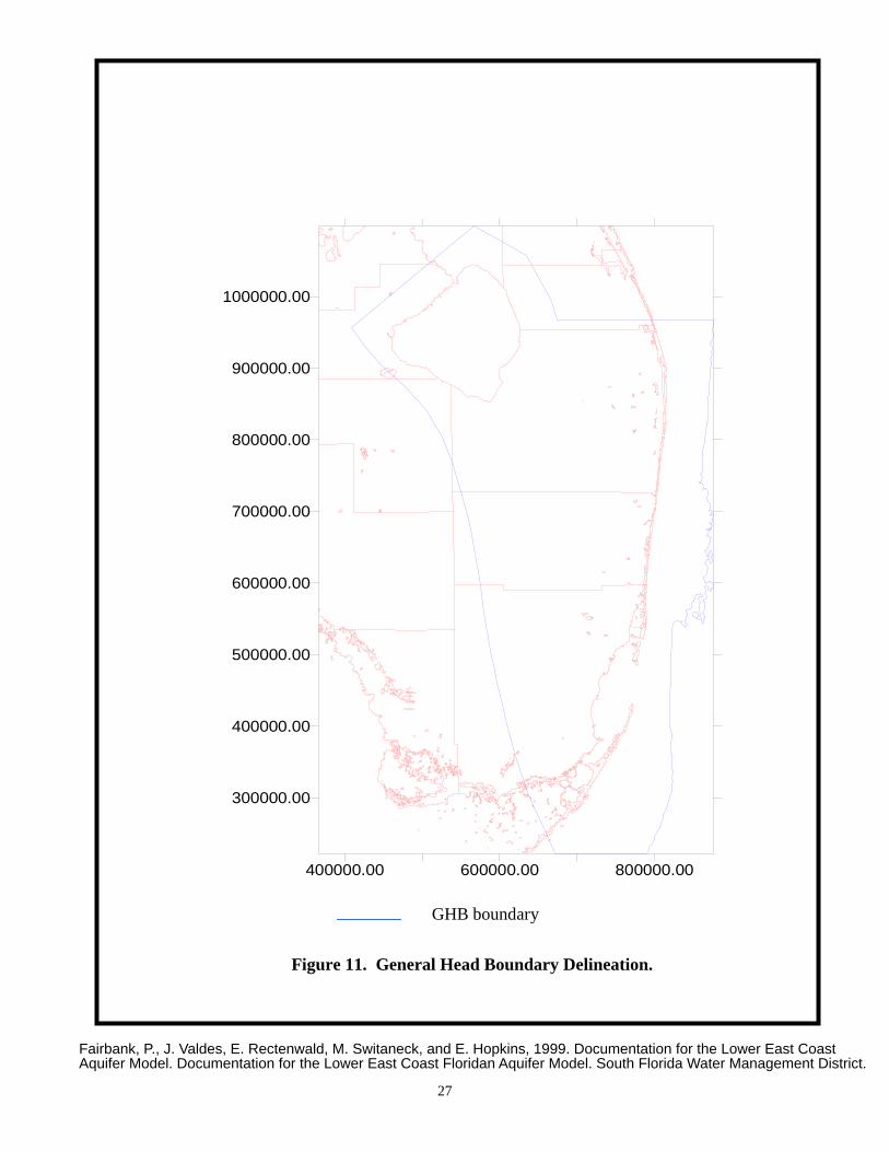
27
400000.00 600000.00 800000.00
300000.00
400000.00
500000.00
600000.00
700000.00
800000.00
900000.00
1000000.00
Figure 11. General Head Boundary Delineation.
GHB boundary
Fairbank, P., J. Valdes, E. Rectenwald, M. Switaneck, and E. Hopkins, 1999. Documentation for the Lower East Coast Aquifer Model. Documentation for the Lower East Coast Floridan Aquifer Model. South Florida Water Management District.
TPA/053320008/SOUTHEAST MODEL TM_07_2006_REV1.DOC 12
Appendix B
Selected Figures and Tables from Documentation of the East Coast Florida model
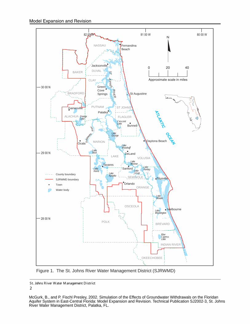
ORANGE
SEMINOLE
BlueCypressLake
LakeWashington
LakeWinder
LakeHarney
LakeJesup
LakeMonroe
LakeWoodruff
LakeGeorge
CrescentLake
LakeApopka
LakeHarris
LakeWeir
OrangeLake
MARION
FLAGLER
ST JOHNS
BAKER
NASSAU
DUVAL
PUTNAM
ALACHUA
Figure 1. The St. Johns River Water Management District (SJRWMD)
ATLANTIC
OCEAN
ST
JO
HN
SR
IVE
R
VOLUSIALAKE
CLAY
Fernandina
Beach
Jacksonville
Green
Cove
Springs St Augustine
Palatka
Gainesville
Ocala
Bunnell
DeLand
Tavares
Orlando
Sanford
Titusville
POLK
OSCEOLA
OKEECHOBEE
INDIAN RIVER
BREVARD
BRADFORD
Ock
lawah
aR
iver
County boundary
SJRWMD boundary
Town
Water body
Daytona Beach
Melbourne
0 20 40
N82 00 W 81 00 W 80 00 W
30 00 N
29 00 N
28 00 N
Approximate scale in miles
St. Johns R iver Water M anagement D istrict
2
Model Expansion and Revision
McGurk, B., and P. Fischl Presley, 2002. Simulation of the Effects of Groundwater Withdrawals on the Floridan Aquifer System in East-Central Florida: Model Expansion and Revision. Technical Publication SJ2002-3, St. Johns River Water Management District, Palatka, FL.

528
BREVARD
ORANGE
VOLUSIA
OSCEOLA
POLK
LAKE
MARION
SEMINOLE
SUMTER
SF
WM
D
SJR
WM
D
SF
WM
DS
WF
WM
D
SW
FW
MD
SJR
WM
D
SFWMD
SJRWMD
St. Johns R iver Water M anagement D istrict
3
Introduction
Figure 2. East-central Florida (ECF) project area — includesa portion of the Southwest Florida WaterManagement District (SWFWMD) and the SouthFlorida Water Management District (SFWMD)
Legend
Road
ECF groundwater flow model boundary
County boundary
SJRWMD boundary
SWFWMD/SFWMD boundary
Water body
N
0 6 12
Approximate scale in miles
95
441
4
98
27
91
1744
42
50
75
4
McGurk, B., and P. Fischl Presley, 2002. Simulation of the Effects of Groundwater Withdrawals on the Floridan Aquifer System in East-Central Florida: Model Expansion and Revision. Technical Publication SJ2002-3, St. Johns River Water Management District, Palatka, FL.

Legend
Rainfall station (see Appendix A)
Surface water data collection site
Floridan aquifer spring
Lake with stage data
Project model boundary
County boundary
SJRWMD boundary
SWFWMD/SFWMD boundary
Water body
N
0 6 12
Approximate scale in miles
Surface water basins
St. Johns River
Ocklawaha River
Atlantic coast
Kissimmee River
Peace River
Withlacoochee River
Wekiva River
BREVARD
ORANGE
VOLUSIA
OSCEOLA
POLK
LAKE
MARION
SU
MT
ER
SEMINOLE
St. Johns R iver Water M anagement D istrict
6
Model Expansion and Revision
Figure 3. Locations of surface-water features, springs,rainfall stations and surface-water data collectionsites
McGurk, B., and P. Fischl Presley, 2002. Simulation of the Effects of Groundwater Withdrawals on the Floridan Aquifer System in East-Central Florida: Model Expansion and Revision. Technical Publication SJ2002-3, St. Johns River Water Management District, Palatka, FL.
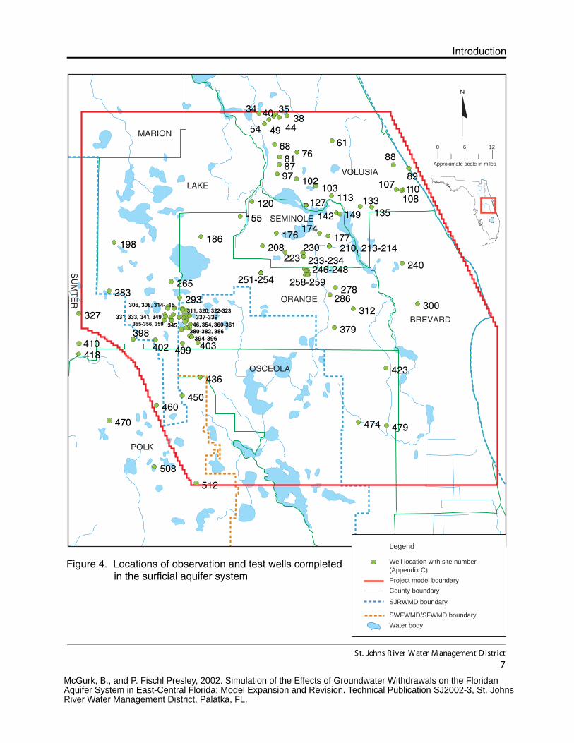
BREVARD
ORANGE
VOLUSIA
OSCEOLA
POLK
LAKE
MARION
SU
MT
ER
SEMINOLE
St. Johns R iver Water M anagement D istrict
7
Introduction
Figure 4. Locations of observation and test wells completed in the surficial aquifer system
N
0 6 12
Approximate scale in miles
Legend
Well location with site number
(Appendix C)
Project model boundary
County boundary
SJRWMD boundary
SWFWMD/SFWMD boundary
Water body
McGurk, B., and P. Fischl Presley, 2002. Simulation of the Effects of Groundwater Withdrawals on the Floridan Aquifer System in East-Central Florida: Model Expansion and Revision. Technical Publication SJ2002-3, St. Johns River Water Management District, Palatka, FL.
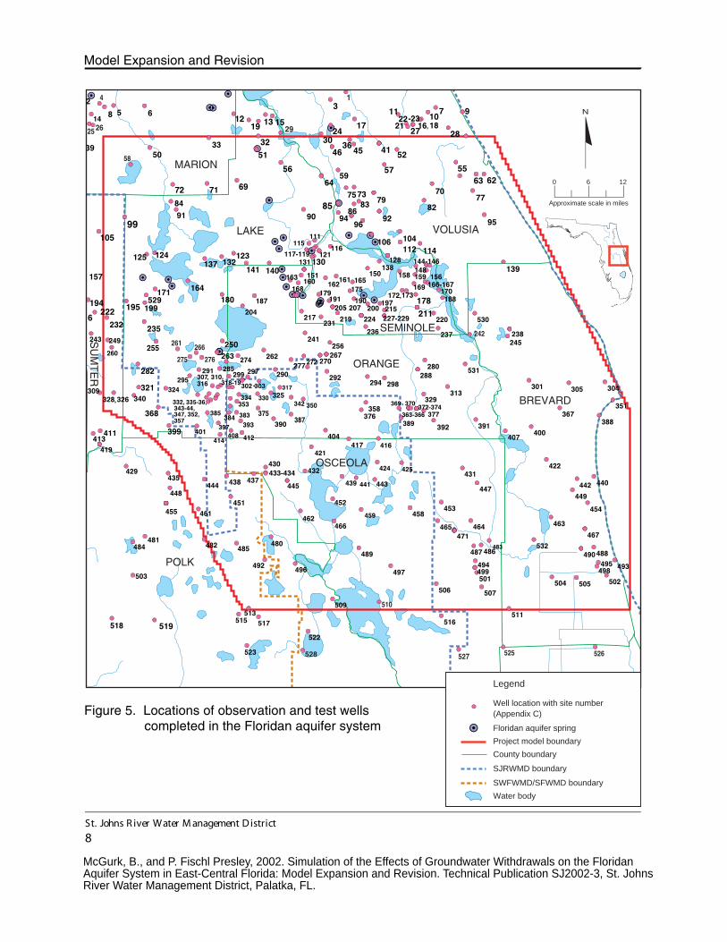
527 525 526
510
2625
4
58
29
1
261
275
266
276
242
BREVARD
ORANGE
VOLUSIA
OSCEOLA
POLK
LAKE
MARION
SU
MT
ER
SEMINOLE
St. Johns R iver Water M anagement D istrict
8
Model Expansion and Revision
Figure 5. Locations of observation and test wells completed in the Floridan aquifer system
Legend
Well location with site number
(Appendix C)
Floridan aquifer spring
Project model boundary
County boundary
SJRWMD boundary
SWFWMD/SFWMD boundary
Water body
N
0 6 12
Approximate scale in miles
McGurk, B., and P. Fischl Presley, 2002. Simulation of the Effects of Groundwater Withdrawals on the Floridan Aquifer System in East-Central Florida: Model Expansion and Revision. Technical Publication SJ2002-3, St. Johns River Water Management District, Palatka, FL.
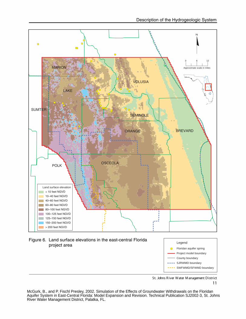
Land surface elevation
< 10 feet NGVD
10–40 feet NGVD
40–60 feet NGVD
60–80 feet NGVD
80–100 feet NGVD
100–125 feet NGVD
125–150 feet NGVD
150–200 feet NGVD
> 200 feet NGVD
BREVARDORANGE
VOLUSIA
OSCEOLAPOLK
LAKE
MARION
SEMINOLE
SUMTER
Figure 6. Land surface elevations in the east-central Floridaproject area
N
0 6 12
Approximate scale in miles
Legend
Floridan aquifer spring
Project model boundary
County boundary
SJRWMD boundary
SWFWMD/SFWMD boundary
St. Johns R iver Water M anagement D istrict
11
Description of the Hydrogeologic System
McGurk, B., and P. Fischl Presley, 2002. Simulation of the Effects of Groundwater Withdrawals on the Floridan Aquifer System in East-Central Florida: Model Expansion and Revision. Technical Publication SJ2002-3, St. Johns River Water Management District, Palatka, FL.

Description of the Hydrogeologic System
St. Johns River Water Management District13
Geologic Series/Stratigraphic Unit
Lithology and Thickness(feet)
HydrostratigraphicUnit
Holocene, Pleistocene/undifferentiated
Interbedded sand, clay, marl, andpeat/0–150
Surficial aquifer system
Pliocene, Miocene/undifferentiated
sediments, HawthornGroup
Interbedded clay, sandy clay, andsand, often phosphatic, with some
phosphatic limestone anddolostone/0–250
Intermediate confiningunit
Upper Eocene/Ocala Limestone
Predominantly soft to hard porouslimestone, minor amounts of hard,
crystalline dolostone/0–300Upper Floridan aquifer—
upper zone
Upper Floridan aquifer—lower zone
Middle semiconfining unitMiddle Eocene/Avon Park Formation
Upper part: predominantly hard,crystalline dolostone with
abundant fractures and solutioncavities/100–200
Middle part: predominantly soft,porous limestone and dolomitic
limestone, with minor amounts ofhard crystalline
dolostone/<100–700
Lower part: soft to hard porouslimestone and hard, fracturedcrystalline dolostone/600–800
Lower Eocene/Oldsmar Formation
Soft to hard porous limestone andhard, fractured crystalline
dolostone; minor amounts of peat,chert, anhydrite, andgypsum/500–1,000
Lower Floridan aquifer
Paleocene/Cedar KeysFormation
Interbedded carbonate rocks andevaporites/500–2,200 Lower confining unit
Figure 7. Geologic and hydrostratigraphic units within the east-central Florida project area
McGurk, B., and P. Fischl Presley, 2002. Simulation of the Effects of Groundwater Withdrawals on the Floridan Aquifer System in East-Central Florida: Model Expansion and Revision. Technical Publication SJ2002-3, St. Johns River Water Management District, Palatka, FL.
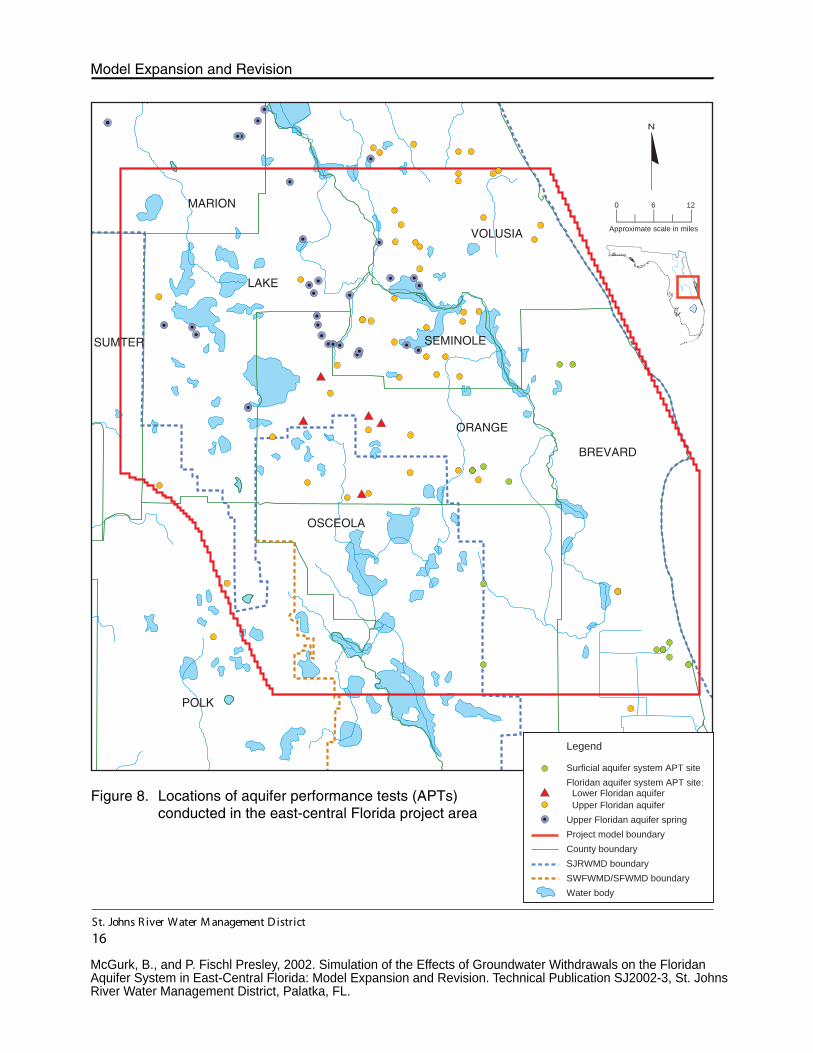
BREVARD
ORANGE
VOLUSIA
OSCEOLA
POLK
LAKE
MARION
SEMINOLESUMTER
Figure 8. Locations of aquifer performance tests (APTs) conducted in the east-central Florida project area
Legend
Surficial aquifer system APT site
Floridan aquifer system APT site: Lower Floridan aquifer
Upper Floridan aquifer
Upper Floridan aquifer spring
Project model boundary
County boundary
SJRWMD boundary
SWFWMD/SFWMD boundary
Water body
St. Johns R iver Water M anagement D istrict
16
Model Expansion and Revision
N
0 6 12
Approximate scale in miles
McGurk, B., and P. Fischl Presley, 2002. Simulation of the Effects of Groundwater Withdrawals on the Floridan Aquifer System in East-Central Florida: Model Expansion and Revision. Technical Publication SJ2002-3, St. Johns River Water Management District, Palatka, FL.
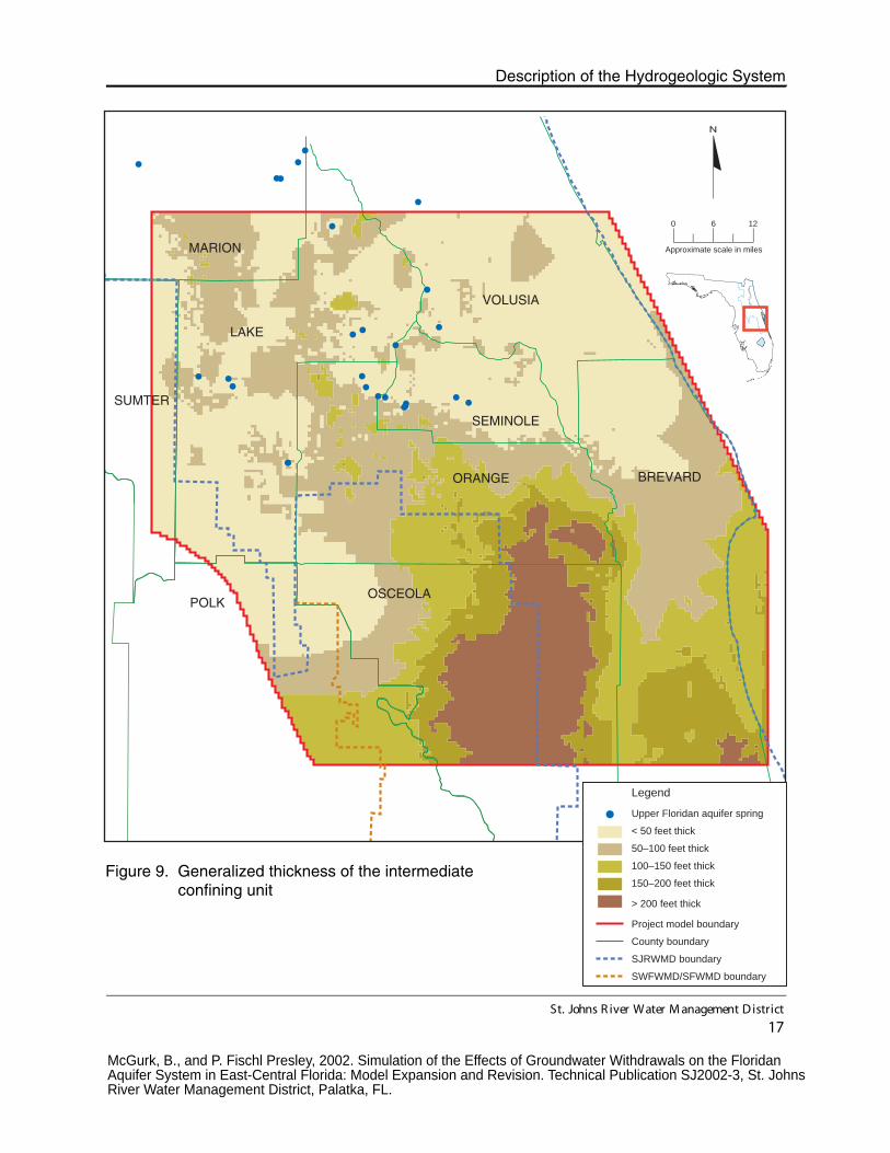
BREVARDORANGE
VOLUSIA
OSCEOLAPOLK
LAKE
MARION
SEMINOLE
SUMTER
Figure 9. Generalized thickness of the intermediateconfining unit
N
0 6 12
Approximate scale in miles
Legend
Upper Floridan aquifer spring
< 50 feet thick
50–100 feet thick
100–150 feet thick
150–200 feet thick
> 200 feet thick
Project model boundary
County boundary
SJRWMD boundary
SWFWMD/SFWMD boundary
St. Johns R iver Water M anagement D istrict
17
Description of the Hydrogeologic System
McGurk, B., and P. Fischl Presley, 2002. Simulation of the Effects of Groundwater Withdrawals on the Floridan Aquifer System in East-Central Florida: Model Expansion and Revision. Technical Publication SJ2002-3, St. Johns River Water Management District, Palatka, FL.
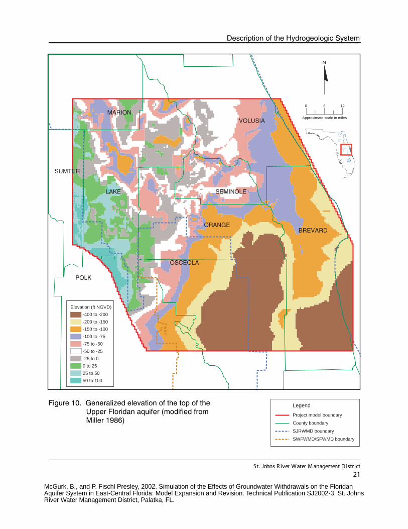
BREVARDORANGE
VOLUSIA
OSCEOLA
POLK
LAKE
MARION
SEMINOLE
SUMTER
Figure 10. Generalized elevation of the top of theUpper Floridan aquifer (modified fromMiller 1986)
N
0 6 12
Approximate scale in miles
Elevation (ft NGVD)
-400 to -200
-200 to -150
-150 to -100
-100 to -75
-75 to -50
-50 to -25
-25 to 0
0 to 25
25 to 50
50 to 100
Legend
Project model boundary
County boundary
SJRWMD boundary
SWFWMD/SFWMD boundary
St. Johns R iver Water M anagement D istrict
21
Description of the Hydrogeologic System
McGurk, B., and P. Fischl Presley, 2002. Simulation of the Effects of Groundwater Withdrawals on the Floridan Aquifer System in East-Central Florida: Model Expansion and Revision. Technical Publication SJ2002-3, St. Johns River Water Management District, Palatka, FL.
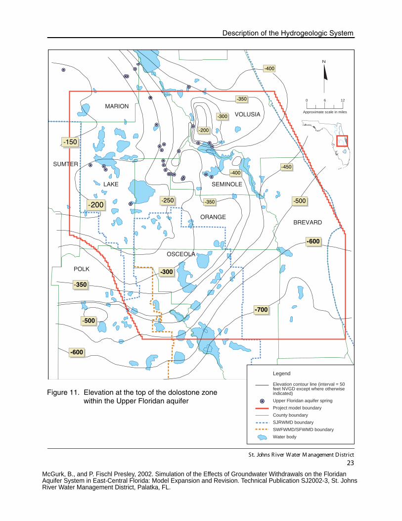
BREVARDORANGE
VOLUSIA
OSCEOLA
POLK
LAKE
MARION
SEMINOLE
SUMTER
St. Johns R iver Water M anagement D istrict
23
Description of the Hydrogeologic System
Figure 11. Elevation at the top of the dolostone zonewithin the Upper Floridan aquifer
Legend
Elevation contour line (interval = 50feet NVGD except where otherwiseindicated)
Upper Floridan aquifer spring
Project model boundary
County boundary
SJRWMD boundary
SWFWMD/SFWMD boundary
Water body
N
0 6 12
Approximate scale in miles
McGurk, B., and P. Fischl Presley, 2002. Simulation of the Effects of Groundwater Withdrawals on the Floridan Aquifer System in East-Central Florida: Model Expansion and Revision. Technical Publication SJ2002-3, St. Johns River Water Management District, Palatka, FL.
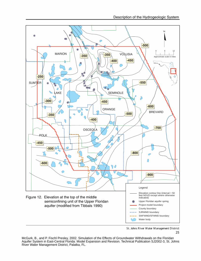
BREVARDORANGE
VOLUSIA
OSCEOLA
POLK
LAKE
MARION
SEMINOLE
SUMTER
St. Johns R iver Water M anagement D istrict
25
Description of the Hydrogeologic System
Figure 12. Elevation at the top of the middlesemiconfining unit of the Upper Floridanaquifer (modified from Tibbals 1990)
N
0 6 12
Approximate scale in miles
Legend
Elevation contour line (interval = 50feet NGVD except where otherwiseindicated)
Upper Floridan aquifer spring
Project model boundary
County boundary
SJRWMD boundary
SWFWMD/SFWMD boundary
Water body
McGurk, B., and P. Fischl Presley, 2002. Simulation of the Effects of Groundwater Withdrawals on the Floridan Aquifer System in East-Central Florida: Model Expansion and Revision. Technical Publication SJ2002-3, St. Johns River Water Management District, Palatka, FL.
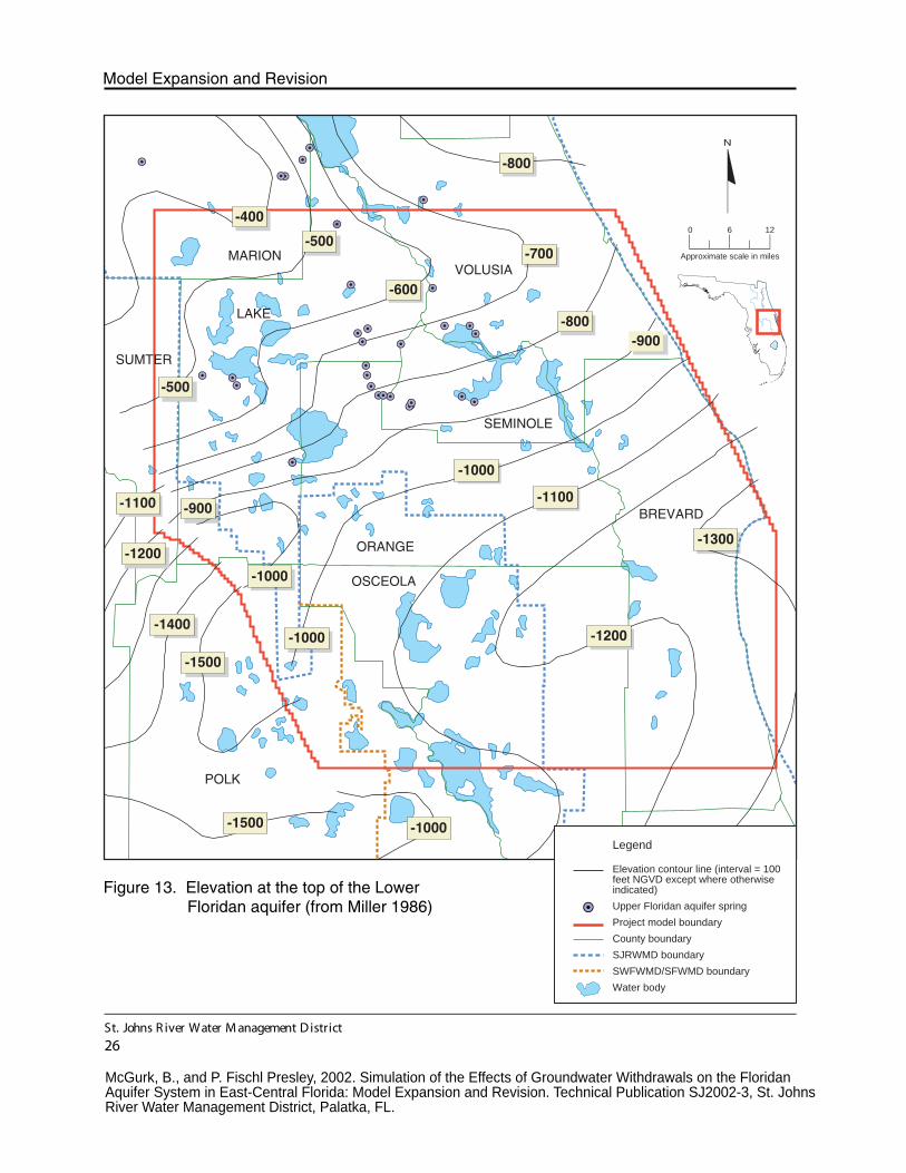
BREVARD
ORANGE
VOLUSIA
OSCEOLA
POLK
LAKE
MARION
SEMINOLE
SUMTER
St. Johns R iver Water M anagement D istrict
26
Model Expansion and Revision
Figure 13. Elevation at the top of the LowerFloridan aquifer (from Miller 1986)
Legend
Elevation contour line (interval = 100feet NGVD except where otherwiseindicated)
Upper Floridan aquifer spring
Project model boundary
County boundary
SJRWMD boundary
SWFWMD/SFWMD boundary
Water body
N
0 6 12
Approximate scale in miles
McGurk, B., and P. Fischl Presley, 2002. Simulation of the Effects of Groundwater Withdrawals on the Floridan Aquifer System in East-Central Florida: Model Expansion and Revision. Technical Publication SJ2002-3, St. Johns River Water Management District, Palatka, FL.
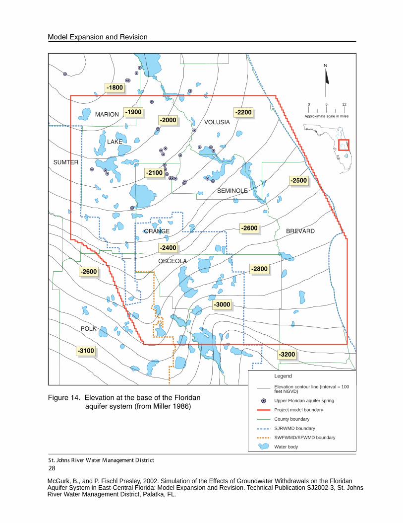
BREVARDORANGE
VOLUSIA
OSCEOLA
POLK
LAKE
MARION
SEMINOLE
SUMTER
St. Johns R iver Water M anagement D istrict
28
Model Expansion and Revision
Figure 14. Elevation at the base of the Floridanaquifer system (from Miller 1986)
Legend
Elevation contour line (interval = 100feet NGVD)
Upper Floridan aquifer spring
Project model boundary
County boundary
SJRWMD boundary
SWFWMD/SFWMD boundary
Water body
N
0 6 12
Approximate scale in miles
McGurk, B., and P. Fischl Presley, 2002. Simulation of the Effects of Groundwater Withdrawals on the Floridan Aquifer System in East-Central Florida: Model Expansion and Revision. Technical Publication SJ2002-3, St. Johns River Water Management District, Palatka, FL.
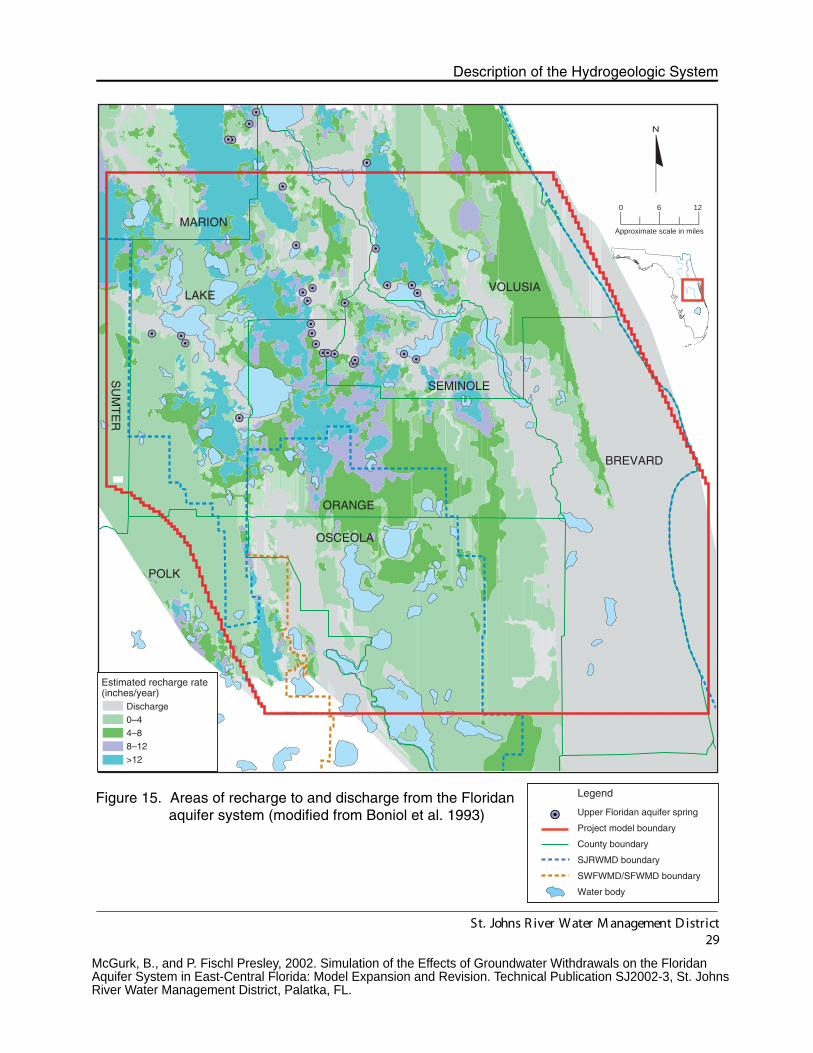
Legend
Upper Floridan aquifer spring
Project model boundary
County boundary
SJRWMD boundary
SWFWMD/SFWMD boundary
Water body
N
0 6 12
Approximate scale in miles
Estimated recharge rate(inches/year)
Discharge0–44–88–12>12
BREVARD
ORANGE
VOLUSIA
OSCEOLA
POLK
LAKE
MARION
SU
MT
ER
SEMINOLE
St. Johns R iver Water M anagement D istrict29
Description of the Hydrogeologic System
Figure 15. Areas of recharge to and discharge from the Floridanaquifer system (modified from Boniol et al. 1993)
McGurk, B., and P. Fischl Presley, 2002. Simulation of the Effects of Groundwater Withdrawals on the Floridan Aquifer System in East-Central Florida: Model Expansion and Revision. Technical Publication SJ2002-3, St. Johns River Water Management District, Palatka, FL.

BREVARD
ORANGE
VOLUSIA
OSCEOLA
POLK
LAKE
MARION
SU
MT
ER
SEMINOLE
St. Johns R iver Water M anagement D istrict
31
Description of the Hydrogeologic System
Figure 16. Locations of drainage wells that recharge theFloridan aquifer system and of abandonedartesian wells
Legend
Drainage well
Abandoned artesian well
Upper Floridan aquifer spring
Project model boundary
County boundary
SJRWMD boundary
SWFWMD/SFWMD boundary
Water body
N
0 6 12
Approximate scale in miles
McGurk, B., and P. Fischl Presley, 2002. Simulation of the Effects of Groundwater Withdrawals on the Floridan Aquifer System in East-Central Florida: Model Expansion and Revision. Technical Publication SJ2002-3, St. Johns River Water Management District, Palatka, FL.
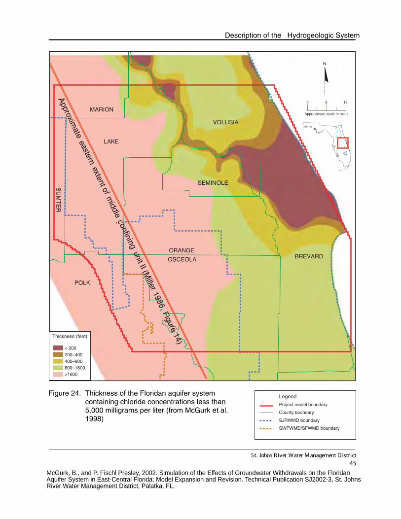
Legend
Project model boundary
County boundary
SJRWMD boundary
SWFWMD/SFWMD boundary
N
0 6 12
Approximate scale in miles
Thickness (feet)
< 200200–400400–800800–1600>1600
BREVARDORANGE
VOLUSIA
OSCEOLA
POLK
LAKE
MARION
SU
MT
ER
SEMINOLE
St. Johns R iver Water M anagement D istrict
45
Description of the Hydrogeologic System
Figure 24. Thickness of the Floridan aquifer systemcontaining chloride concentrations less than5,000 milligrams per liter (from McGurk et al.1998)
McGurk, B., and P. Fischl Presley, 2002. Simulation of the Effects of Groundwater Withdrawals on the Floridan Aquifer System in East-Central Florida: Model Expansion and Revision. Technical Publication SJ2002-3, St. Johns River Water Management District, Palatka, FL.
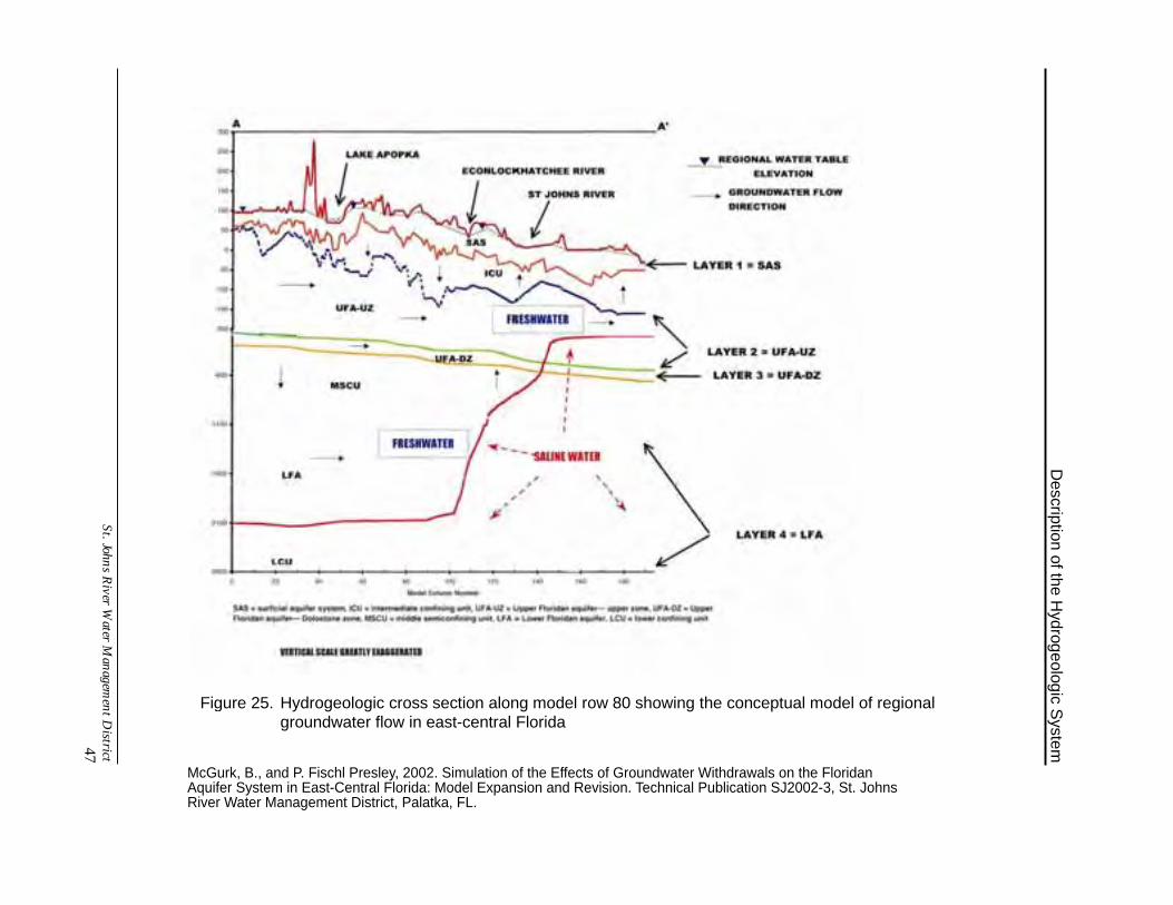
Description of the H
ydrogeologic System
St.JohnsR
iverW
aterM
anagementD
istrict47
Figure 25. Hydrogeologic cross section along model row 80 showing the conceptual model of regional groundwater flow in east-central Florida
McGurk, B., and P. Fischl Presley, 2002. Simulation of the Effects of Groundwater Withdrawals on the Floridan Aquifer System in East-Central Florida: Model Expansion and Revision. Technical Publication SJ2002-3, St. Johns River Water Management District, Palatka, FL.

BREVARD
ORANGE
VOLUSIA
OSCEOLA
POLK
LAKE
MARION
SEMINOLE
SUMTER
St. Johns R iver Water M anagement D istrict
50
Model Expansion and Revision
Figure 26. East-central Florida regional model domainshowing inactive areas and layer 1 grid celldesignations
Legend
Inactive for all layers
Location of cross section shownby Figure 25 (model row 80)
County boundary
SJRWMD boundary
SWFWMD/SFWMD boundary
N
0 6 12
Approximate scale in miles
Layer 1 grid cell designations
Constant-head cell
Variable-head cell
Variable-head cell with River Package
McGurk, B., and P. Fischl Presley, 2002. Simulation of the Effects of Groundwater Withdrawals on the Floridan Aquifer System in East-Central Florida: Model Expansion and Revision. Technical Publication SJ2002-3, St. Johns River Water Management District, Palatka, FL.

N
0 6 12
Approximate scale in miles
Legend
Layer 2 grid cell designationsInactiveVariable-head cellVariable-head cell with River PackageVariable-head cell with general-head boundaryVariable-head cell with Drain Package
County boundary
SJRWMD boundary
SWFWMD/SFWMD boundary
St. Johns R iver Water M anagement D istrict
52
Model Expansion and Revision
Figure 27. Layer 2 lateral boundary conditions andlocations of River Package and DrainPackage cells
BREVARD
ORANGE
VOLUSIA
OSCEOLA
POLK
LAKE
MARION
SU
MT
ER
SEMINOLE
McGurk, B., and P. Fischl Presley, 2002. Simulation of the Effects of Groundwater Withdrawals on the Floridan Aquifer System in East-Central Florida: Model Expansion and Revision. Technical Publication SJ2002-3, St. Johns River Water Management District, Palatka, FL.
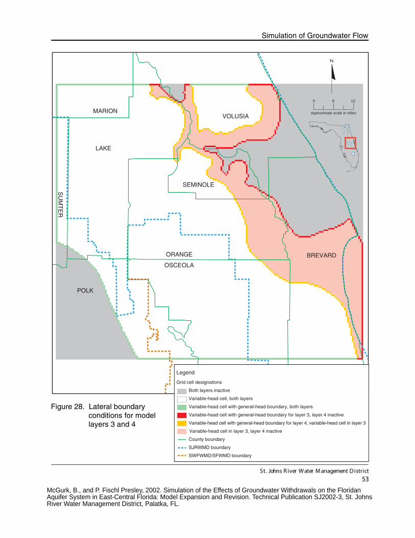
BREVARDORANGE
VOLUSIA
OSCEOLA
POLK
LAKE
MARION
SU
MT
ER
SEMINOLE
N
0 6 12
Approximate scale in miles
Legend
Grid cell designations
Both layers inactive
Variable-head cell, both layers
Variable-head cell with general-head boundary, both layers
Variable-head cell with general-head boundary for layer 3, layer 4 inactive
Variable-head cell with general-head boundary for layer 4, variable-head cell in layer 3
Variable-head cell in layer 3, layer 4 inactive
County boundary
SJRWMD boundary
SWFWMD/SFWMD boundary
St. Johns R iver Water M anagement D istrict
53
Simulation of Groundwater Flow
Figure 28. Lateral boundaryconditions for modellayers 3 and 4
McGurk, B., and P. Fischl Presley, 2002. Simulation of the Effects of Groundwater Withdrawals on the Floridan Aquifer System in East-Central Florida: Model Expansion and Revision. Technical Publication SJ2002-3, St. Johns River Water Management District, Palatka, FL.
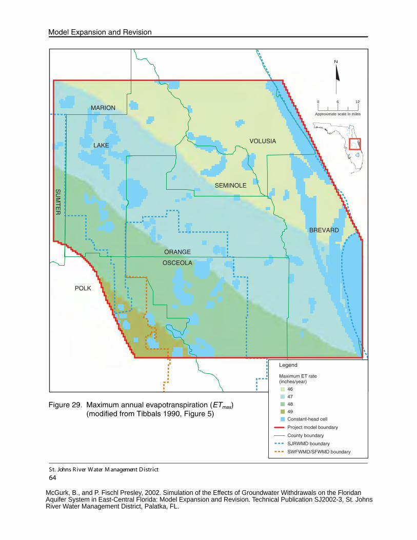
N
0 6 12
Approximate scale in miles
Legend
Maximum ET rate(inches/year)
46
47
48
49
Constant-head cell
Project model boundary
County boundary
SJRWMD boundary
SWFWMD/SFWMD boundary
St. Johns R iver Water M anagement D istrict
64
Model Expansion and Revision
Figure 29. Maximum annual evapotranspiration (ETmax) (modified from Tibbals 1990, Figure 5)
BREVARD
ORANGE
VOLUSIA
OSCEOLA
POLK
LAKE
MARION
SU
MT
ER
SEMINOLE
McGurk, B., and P. Fischl Presley, 2002. Simulation of the Effects of Groundwater Withdrawals on the Floridan Aquifer System in East-Central Florida: Model Expansion and Revision. Technical Publication SJ2002-3, St. Johns River Water Management District, Palatka, FL.
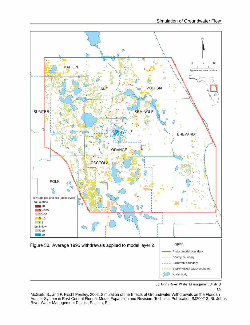
BREVARD
ORANGE
VOLUSIA
OSCEOLA
POLK
LAKE
MARION
SEMINOLESUMTER
Flow rate per grid cell (inches/year)
Net outflow
> 100
50–100
10–50
5–10
< 5
Net inflow
< 10
> 10
POLK
St. Johns R iver Water M anagement D istrict
69
Simulation of Groundwater Flow
Figure 30. Average 1995 withdrawals applied to model layer 2 Legend
Project model boundary
County boundary
SJRWMD boundary
SWFWMD/SFWMD boundary
Water body
N
0 6 12
Approximate scale in miles
McGurk, B., and P. Fischl Presley, 2002. Simulation of the Effects of Groundwater Withdrawals on the Floridan Aquifer System in East-Central Florida: Model Expansion and Revision. Technical Publication SJ2002-3, St. Johns River Water Management District, Palatka, FL.
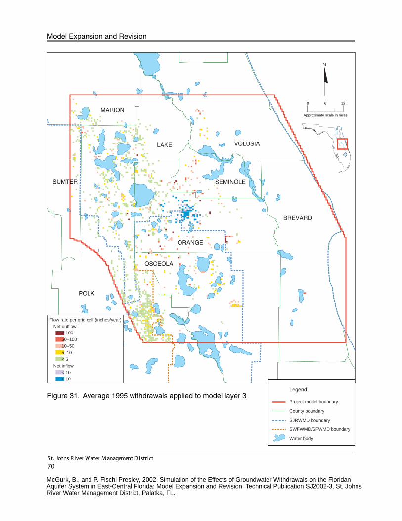
BREVARD
ORANGE
VOLUSIA
OSCEOLA
POLK
LAKE
MARION
SEMINOLESUMTER
Flow rate per grid cell (inches/year)
Net outflow
> 100
50–100
10–50
5–10
< 5
Net inflow
< 10
> 10
POLK
St. Johns R iver Water M anagement D istrict
70
Model Expansion and Revision
Figure 31. Average 1995 withdrawals applied to model layer 3Legend
Project model boundary
County boundary
SJRWMD boundary
SWFWMD/SFWMD boundary
Water body
N
0 6 12
Approximate scale in miles
McGurk, B., and P. Fischl Presley, 2002. Simulation of the Effects of Groundwater Withdrawals on the Floridan Aquifer System in East-Central Florida: Model Expansion and Revision. Technical Publication SJ2002-3, St. Johns River Water Management District, Palatka, FL.
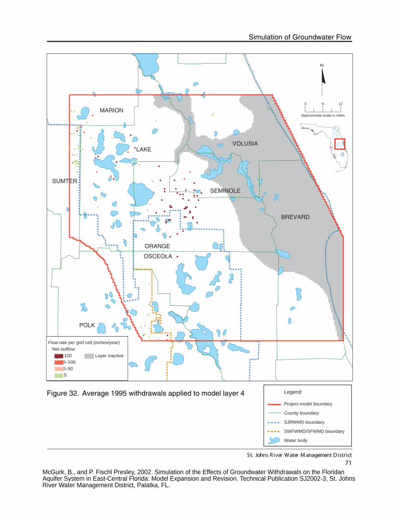
BREVARD
ORANGE
VOLUSIA
OSCEOLA
POLK
LAKE
MARION
SEMINOLE
SUMTER
Flow rate per grid cell (inches/year)
Net outflow
> 100
50–100
10–50
< 5
Legend
Project model boundary
County boundary
SJRWMD boundary
SWFWMD/SFWMD boundary
Water body
Layer inactive
St. Johns R iver Water M anagement D istrict
71
Simulation of Groundwater Flow
Figure 32. Average 1995 withdrawals applied to model layer 4
N
0 6 12
Approximate scale in miles
McGurk, B., and P. Fischl Presley, 2002. Simulation of the Effects of Groundwater Withdrawals on the Floridan Aquifer System in East-Central Florida: Model Expansion and Revision. Technical Publication SJ2002-3, St. Johns River Water Management District, Palatka, FL.
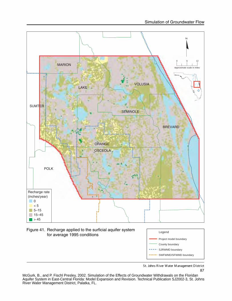
BREVARD
ORANGE
VOLUSIA
OSCEOLA
POLK
LAKE
MARION
SEMINOLE
SUMTER
Recharge rate(inches/year) 0 < 5 5–15 15–45 > 45
St. Johns R iver Water M anagement D istrict
87
Simulation of Groundwater Flow
Figure 41. Recharge applied to the surficial aquifer system for average 1995 conditions
Legend
Project model boundary
County boundary
SJRWMD boundary
SWFWMD/SFWMD boundary
N
0 6 12
Approximate scale in miles
McGurk, B., and P. Fischl Presley, 2002. Simulation of the Effects of Groundwater Withdrawals on the Floridan Aquifer System in East-Central Florida: Model Expansion and Revision. Technical Publication SJ2002-3, St. Johns River Water Management District, Palatka, FL.

BREVARD
ORANGE
VOLUSIA
OSCEOLA
POLK
LAKE
MARION
SEMINOLE
SUMTER
Vertical hydraulic conductivity(feet/day)
< 0.002
0.002–0.02
> 0.02
St. Johns R iver Water M anagement D istrict
127
Simulation of Groundwater Flow
Figure 65. Calibrated vertical hydraulic conductivity of theintermediate confining unit
Legend
Upper Floridan aquifer spring
Layer 2 inactive
Project model boundary
County boundary
SJRWMD boundary
SWFWMD/SFWMD boundary
N
0 6 12
Approximate scale in miles
McGurk, B., and P. Fischl Presley, 2002. Simulation of the Effects of Groundwater Withdrawals on the Floridan Aquifer System in East-Central Florida: Model Expansion and Revision. Technical Publication SJ2002-3, St. Johns River Water Management District, Palatka, FL.
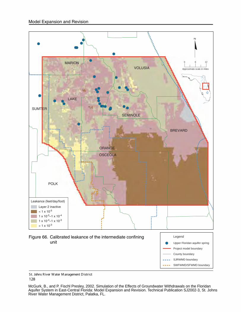
BREVARD
ORANGE
VOLUSIA
OSCEOLA
POLK
LAKE
MARION
SEMINOLE
SUMTER
Leakance (feet/day/foot)
Layer 2 inactive
< 1 x 10⁻⁵
1 x 10⁻⁵–1 x 10⁻⁴
1 x 10⁻⁴–1 x 10⁻³
> 1 x 10⁻³
St. Johns R iver Water M anagement D istrict
128
Model Expansion and Revision
Figure 66. Calibrated leakance of the intermediate confiningunit
Legend
Upper Floridan aquifer spring
Project model boundary
County boundary
SJRWMD boundary
SWFWMD/SFWMD boundary
N
0 6 12
Approximate scale in miles
McGurk, B., and P. Fischl Presley, 2002. Simulation of the Effects of Groundwater Withdrawals on the Floridan Aquifer System in East-Central Florida: Model Expansion and Revision. Technical Publication SJ2002-3, St. Johns River Water Management District, Palatka, FL.
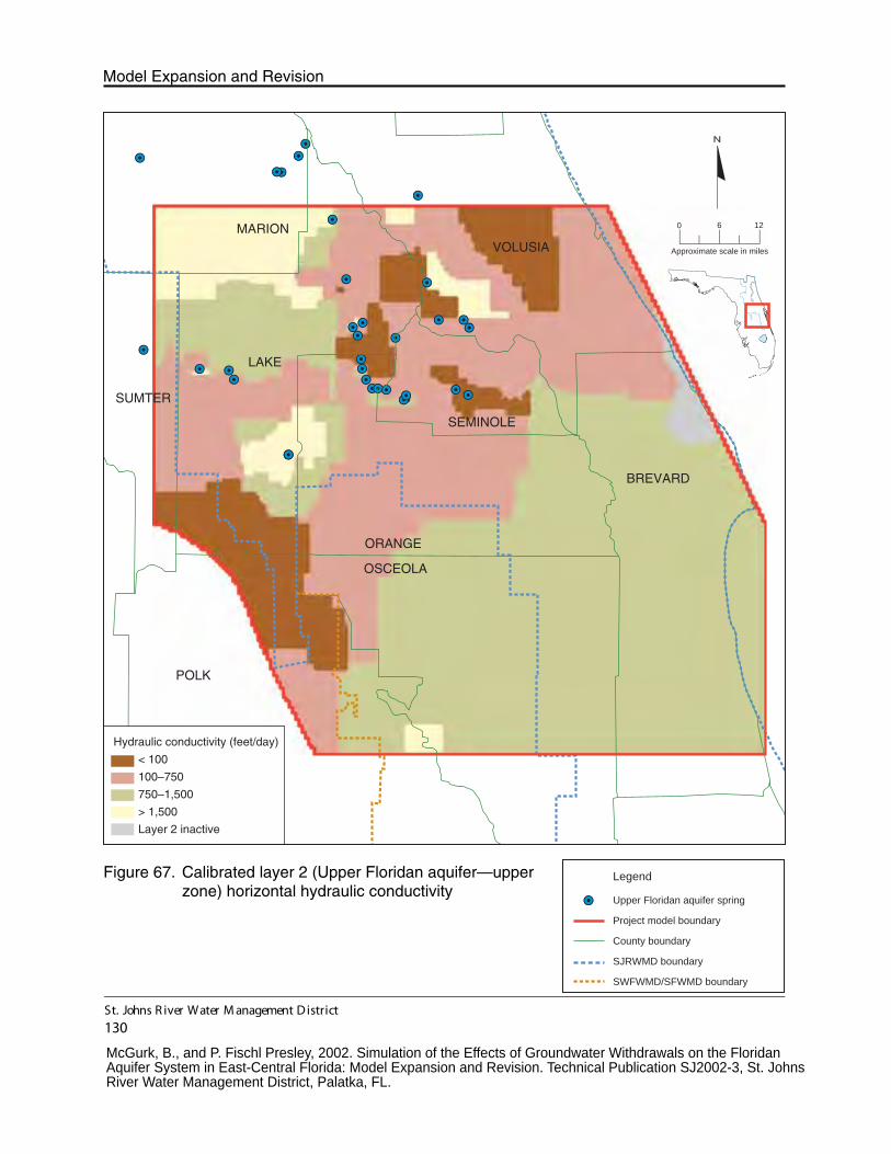
BREVARD
ORANGE
VOLUSIA
OSCEOLA
POLK
LAKE
MARION
SEMINOLE
SUMTER
Hydraulic conductivity (feet/day)
< 100
100–750
750–1,500
> 1,500
Layer 2 inactive
St. Johns R iver Water M anagement D istrict
130
Model Expansion and Revision
Figure 67. Calibrated layer 2 (Upper Floridan aquifer—upperzone) horizontal hydraulic conductivity
Legend
Upper Floridan aquifer spring
Project model boundary
County boundary
SJRWMD boundary
SWFWMD/SFWMD boundary
N
0 6 12
Approximate scale in miles
McGurk, B., and P. Fischl Presley, 2002. Simulation of the Effects of Groundwater Withdrawals on the Floridan Aquifer System in East-Central Florida: Model Expansion and Revision. Technical Publication SJ2002-3, St. Johns River Water Management District, Palatka, FL.
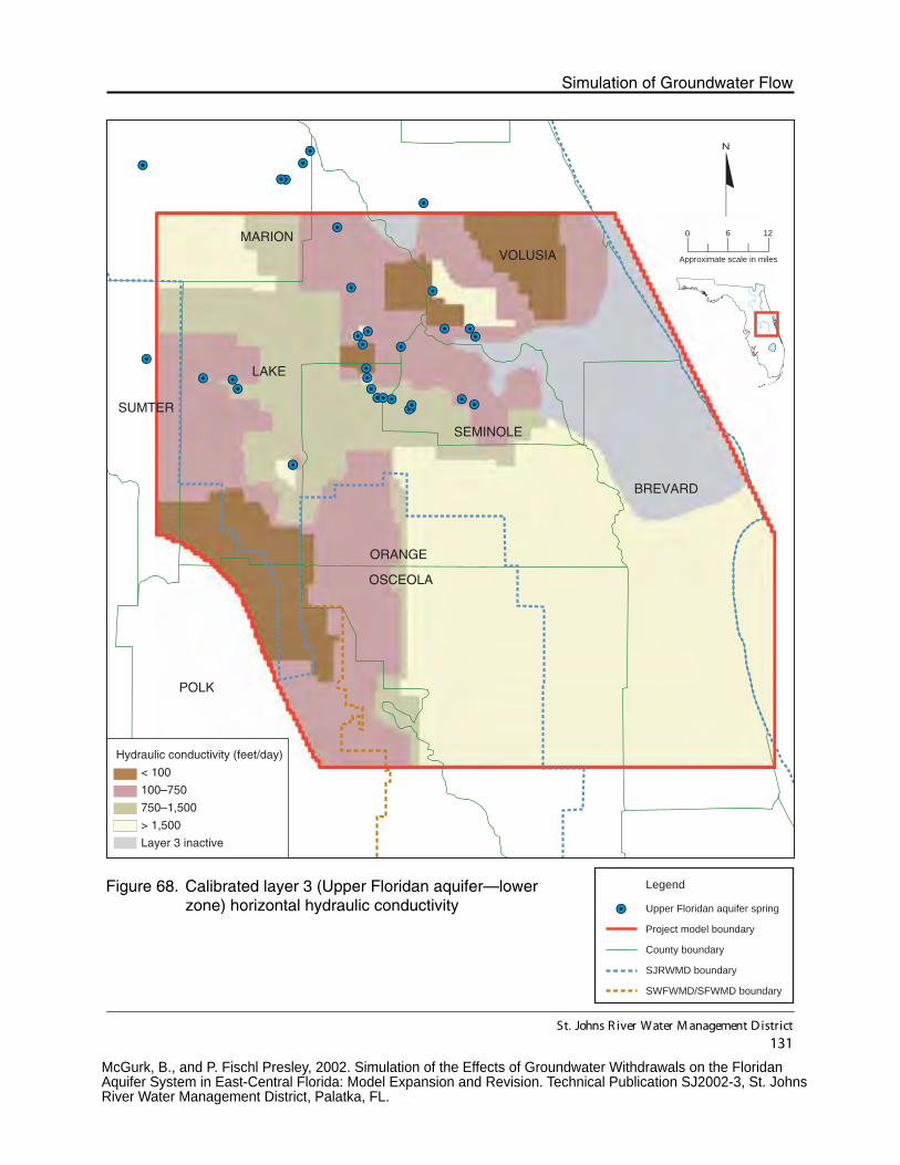
BREVARD
ORANGE
VOLUSIA
OSCEOLA
POLK
LAKE
MARION
SEMINOLE
SUMTER
Hydraulic conductivity (feet/day)
< 100
100–750
750–1,500
> 1,500
Layer 3 inactive
St. Johns R iver Water M anagement D istrict
131
Simulation of Groundwater Flow
Figure 68. Calibrated layer 3 (Upper Floridan aquifer—lowerzone) horizontal hydraulic conductivity
Legend
Upper Floridan aquifer spring
Project model boundary
County boundary
SJRWMD boundary
SWFWMD/SFWMD boundary
N
0 6 12
Approximate scale in miles
McGurk, B., and P. Fischl Presley, 2002. Simulation of the Effects of Groundwater Withdrawals on the Floridan Aquifer System in East-Central Florida: Model Expansion and Revision. Technical Publication SJ2002-3, St. Johns River Water Management District, Palatka, FL.

BREVARD
ORANGE
VOLUSIA
OSCEOLA
POLK
LAKE
MARION
SEMINOLE
SUMTER
Transmissivity (square feet/day)
< 25,000
25,000–150,000
150,000–750,000
> 750,000
Layer 2 inactive
St. Johns R iver Water M anagement D istrict
132
Model Expansion and Revision
Figure 69. Calibrated transmissivity of the Upper Floridanaquifer (layers 2 and 3)
Legend
Upper Floridan aquifer spring
Project model boundary
County boundary
SJRWMD boundary
SWFWMD/SFWMD boundary
N
0 6 12
Approximate scale in miles
McGurk, B., and P. Fischl Presley, 2002. Simulation of the Effects of Groundwater Withdrawals on the Floridan Aquifer System in East-Central Florida: Model Expansion and Revision. Technical Publication SJ2002-3, St. Johns River Water Management District, Palatka, FL.
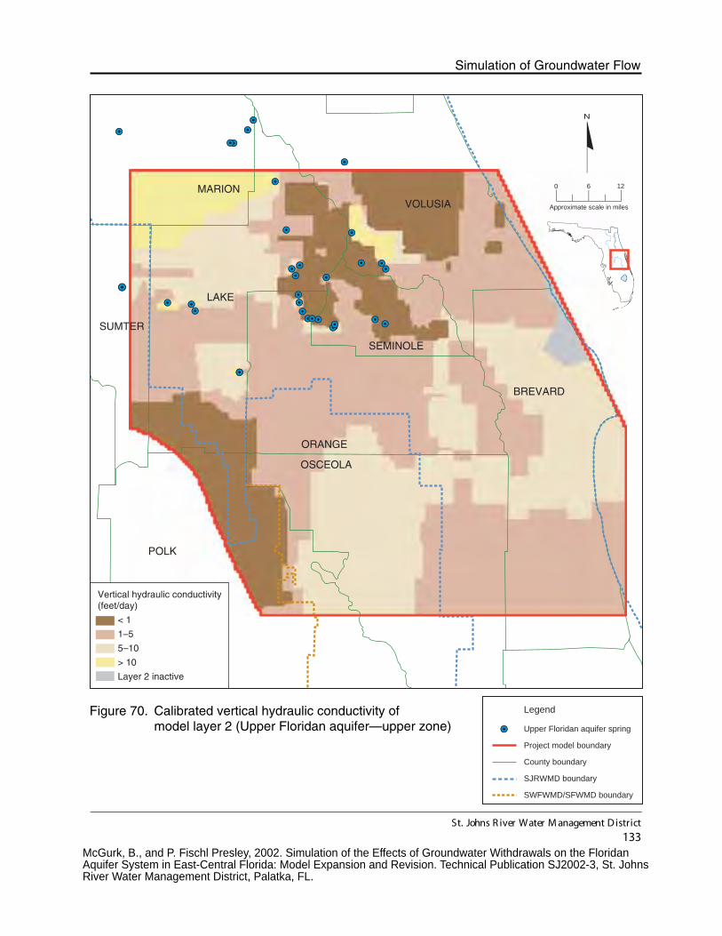
BREVARD
ORANGE
VOLUSIA
OSCEOLA
POLK
LAKE
MARION
SEMINOLE
SUMTER
Vertical hydraulic conductivity(feet/day)
< 1
1–5
5–10
> 10
Layer 2 inactive
St. Johns R iver Water M anagement D istrict
133
Simulation of Groundwater Flow
Figure 70. Calibrated vertical hydraulic conductivity ofmodel layer 2 (Upper Floridan aquifer—upper zone)
Legend
Upper Floridan aquifer spring
Project model boundary
County boundary
SJRWMD boundary
SWFWMD/SFWMD boundary
N
0 6 12
Approximate scale in miles
McGurk, B., and P. Fischl Presley, 2002. Simulation of the Effects of Groundwater Withdrawals on the Floridan Aquifer System in East-Central Florida: Model Expansion and Revision. Technical Publication SJ2002-3, St. Johns River Water Management District, Palatka, FL.
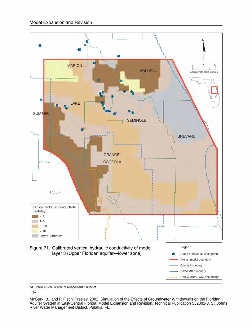
BREVARD
ORANGE
VOLUSIA
OSCEOLA
POLK
LAKE
MARION
SEMINOLE
SUMTER
Vertical hydraulic conductivity(feet/day)
< 1
1–5
5–10
> 10
Layer 3 inactive
St. Johns R iver Water M anagement D istrict
134
Model Expansion and Revision
Figure 71. Calibrated vertical hydraulic conductivity of modellayer 3 (Upper Floridan aquifer—lower zone)
Legend
Upper Floridan aquifer spring
Project model boundary
County boundary
SJRWMD boundary
SWFWMD/SFWMD boundary
N
0 6 12
Approximate scale in miles
McGurk, B., and P. Fischl Presley, 2002. Simulation of the Effects of Groundwater Withdrawals on the Floridan Aquifer System in East-Central Florida: Model Expansion and Revision. Technical Publication SJ2002-3, St. Johns River Water Management District, Palatka, FL.

BREVARD
ORANGE
VOLUSIA
OSCEOLA
POLK
LAKE
MARION
SEMINOLE
SUMTER
Leakance (feet/day/foot)
0.001–0.01
0.01–0.1
> 0.1
Layer 3 inactive
St. Johns R iver Water M anagement D istrict
136
Model Expansion and Revision
Figure 72. Calibrated leakance between Upper Floridan aquiferlayers 2 and 3
Legend
Upper Floridan aquifer spring
Project model boundary
County boundary
SJRWMD boundary
SWFWMD/SFWMD boundary
N
0 6 12
Approximate scale in miles
McGurk, B., and P. Fischl Presley, 2002. Simulation of the Effects of Groundwater Withdrawals on the Floridan Aquifer System in East-Central Florida: Model Expansion and Revision. Technical Publication SJ2002-3, St. Johns River Water Management District, Palatka, FL.
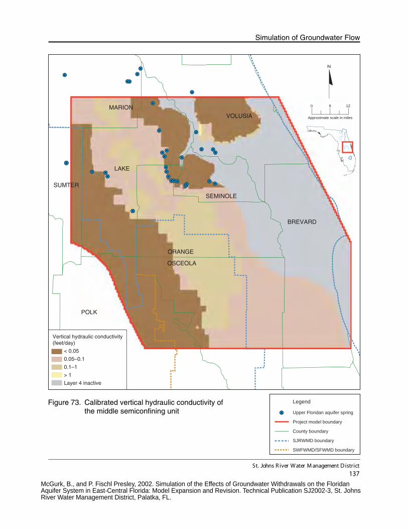
BREVARD
ORANGE
VOLUSIA
OSCEOLA
POLK
LAKE
MARION
SEMINOLE
SUMTER
Vertical hydraulic conductivity(feet/day)
< 0.05
0.05–0.1
0.1–1
\ > 1
Layer 4 inactive
St. Johns R iver Water M anagement D istrict
137
Simulation of Groundwater Flow
Figure 73. Calibrated vertical hydraulic conductivity ofthe middle semiconfining unit
Legend
Upper Floridan aquifer spring
Project model boundary
County boundary
SJRWMD boundary
SWFWMD/SFWMD boundary
N
0 6 12
Approximate scale in miles
McGurk, B., and P. Fischl Presley, 2002. Simulation of the Effects of Groundwater Withdrawals on the Floridan Aquifer System in East-Central Florida: Model Expansion and Revision. Technical Publication SJ2002-3, St. Johns River Water Management District, Palatka, FL.

BREVARD
ORANGE
VOLUSIA
OSCEOLA
POLK
LAKE
MARION
SEMINOLE
SUMTER
Leakance (feet/day/foot)
< 0.00005
0.00005–0.0001
0.0001–0.001
> 0.001
Layer 4 inactive
St. Johns R iver Water M anagement D istrict
138
Model Expansion and Revision
Figure 74. Calibrated leakance of the middle semiconfining unit Legend
Upper Floridan aquifer spring
Project model boundary
County boundary
SJRWMD boundary
SWFWMD/SFWMD boundary
N
0 6 12
Approximate scale in miles
McGurk, B., and P. Fischl Presley, 2002. Simulation of the Effects of Groundwater Withdrawals on the Floridan Aquifer System in East-Central Florida: Model Expansion and Revision. Technical Publication SJ2002-3, St. Johns River Water Management District, Palatka, FL.
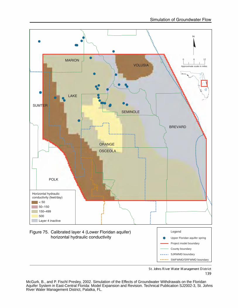
BREVARD
ORANGE
VOLUSIA
OSCEOLA
POLK
LAKE
MARION
SEMINOLE
SUMTER
Horizontal hydraulicconductivity (feet/day)
< 50
50–150
150–499
500
Layer 4 inactive
St. Johns R iver Water M anagement D istrict
139
Simulation of Groundwater Flow
Figure 75. Calibrated layer 4 (Lower Floridan aquifer)horizontal hydraulic conductivity
Legend
Upper Floridan aquifer spring
Project model boundary
County boundary
SJRWMD boundary
SWFWMD/SRFWMD boundary
N
0 6 12
Approximate scale in miles
McGurk, B., and P. Fischl Presley, 2002. Simulation of the Effects of Groundwater Withdrawals on the Floridan Aquifer System in East-Central Florida: Model Expansion and Revision. Technical Publication SJ2002-3, St. Johns River Water Management District, Palatka, FL.

BREVARD
ORANGE
VOLUSIA
OSCEOLA
POLK
LAKE
MARION
SEMINOLE
SUMTER
Transmissivity (square feet/day)
< 25,000
25,000–150,000
150,000–750,000
Layer 4 inactive
St. Johns R iver Water M anagement D istrict
140
Model Expansion and Revision
Figure 76. Calibrated transmissivity of the Lower Floridanaquifer (layer 4)
Legend
Upper Floridan aquifer spring
Project model boundary
County boundary
SJRWMD boundary
SWFWMD/SFWMD boundary
N
0 6 12
Approximate scale in miles
McGurk, B., and P. Fischl Presley, 2002. Simulation of the Effects of Groundwater Withdrawals on the Floridan Aquifer System in East-Central Florida: Model Expansion and Revision. Technical Publication SJ2002-3, St. Johns River Water Management District, Palatka, FL.
TPA/053320008/SOUTHEAST MODEL TM_07_2006_REV1.DOC 13
Appendix C
Selected Figures from Documentation of the Lee County, Florida model

Bower, R.F., K.M. Adams and J.I. Restrepo, 1990. A Three-Dimensional Finite Difference Ground Water Model of
Lee County, Florida. Technical Publication 90-01, South Florida Water Management District, West Palm Beach, FL.

Bower, R.F., K.M. Adams and J.I. Restrepo, 1990. A Three-Dimensional Finite Difference Ground Water Model of
Lee County, Florida. Technical Publication 90-01, South Florida Water Management District, West Palm Beach, FL.
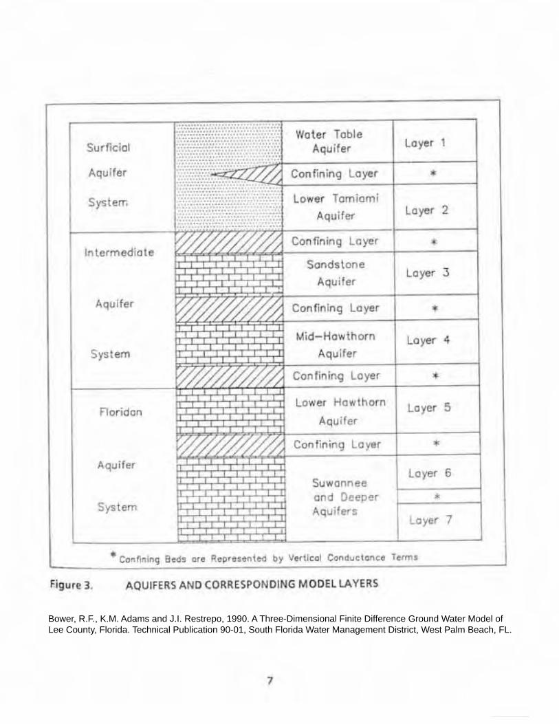
Bower, R.F., K.M. Adams and J.I. Restrepo, 1990. A Three-Dimensional Finite Difference Ground Water Model of
Lee County, Florida. Technical Publication 90-01, South Florida Water Management District, West Palm Beach, FL.

Bower, R.F., K.M. Adams and J.I. Restrepo, 1990. A Three-Dimensional Finite Difference Ground Water Model of
Lee County, Florida. Technical Publication 90-01, South Florida Water Management District, West Palm Beach, FL.

Bower, R.F., K.M. Adams and J.I. Restrepo, 1990. A Three-Dimensional Finite Difference Ground Water Model of
Lee County, Florida. Technical Publication 90-01, South Florida Water Management District, West Palm Beach, FL.
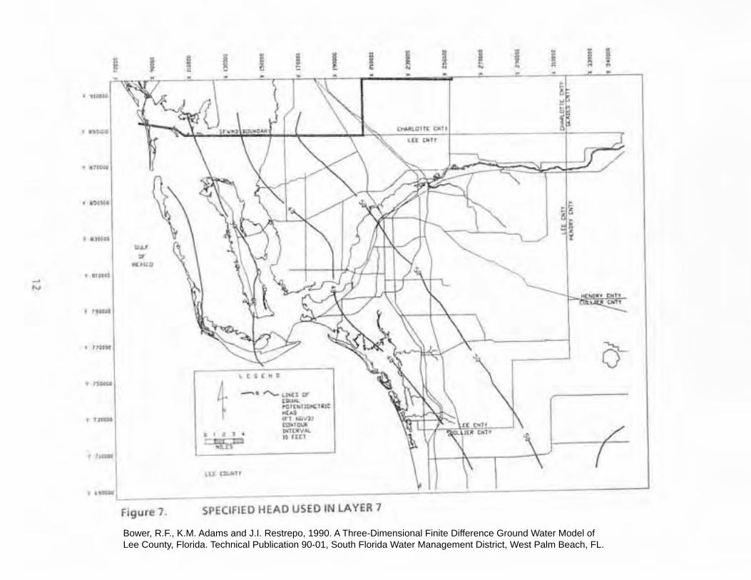
Bower, R.F., K.M. Adams and J.I. Restrepo, 1990. A Three-Dimensional Finite Difference Ground Water Model of
Lee County, Florida. Technical Publication 90-01, South Florida Water Management District, West Palm Beach, FL.

Bower, R.F., K.M. Adams and J.I. Restrepo, 1990. A Three-Dimensional Finite Difference Ground Water Model of
Lee County, Florida. Technical Publication 90-01, South Florida Water Management District, West Palm Beach, FL.
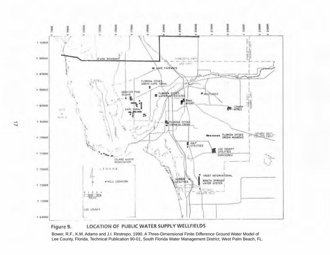
Bower, R.F., K.M. Adams and J.I. Restrepo, 1990. A Three-Dimensional Finite Difference Ground Water Model of
Lee County, Florida. Technical Publication 90-01, South Florida Water Management District, West Palm Beach, FL.

Bower, R.F., K.M. Adams and J.I. Restrepo, 1990. A Three-Dimensional Finite Difference Ground Water Model of
Lee County, Florida. Technical Publication 90-01, South Florida Water Management District, West Palm Beach, FL.

Bower, R.F., K.M. Adams and J.I. Restrepo, 1990. A Three-Dimensional Finite Difference Ground Water Model of
Lee County, Florida. Technical Publication 90-01, South Florida Water Management District, West Palm Beach, FL.

Bower, R.F., K.M. Adams and J.I. Restrepo, 1990. A Three-Dimensional Finite Difference Ground Water Model of
Lee County, Florida. Technical Publication 90-01, South Florida Water Management District, West Palm Beach, FL.

Bower, R.F., K.M. Adams and J.I. Restrepo, 1990. A Three-Dimensional Finite Difference Ground Water Model of
Lee County, Florida. Technical Publication 90-01, South Florida Water Management District, West Palm Beach, FL.

Bower, R.F., K.M. Adams and J.I. Restrepo, 1990. A Three-Dimensional Finite Difference Ground Water Model of
Lee County, Florida. Technical Publication 90-01, South Florida Water Management District, West Palm Beach, FL.
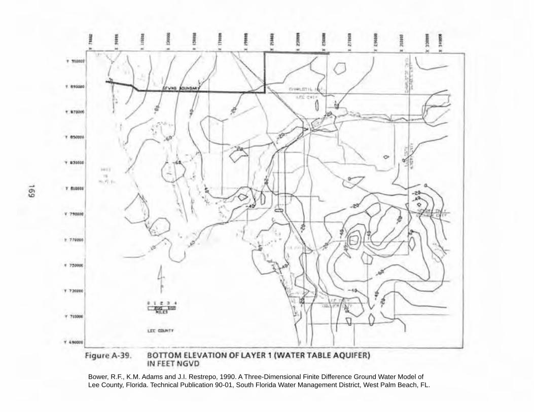
Bower, R.F., K.M. Adams and J.I. Restrepo, 1990. A Three-Dimensional Finite Difference Ground Water Model of
Lee County, Florida. Technical Publication 90-01, South Florida Water Management District, West Palm Beach, FL.

Bower, R.F., K.M. Adams and J.I. Restrepo, 1990. A Three-Dimensional Finite Difference Ground Water Model of
Lee County, Florida. Technical Publication 90-01, South Florida Water Management District, West Palm Beach, FL.
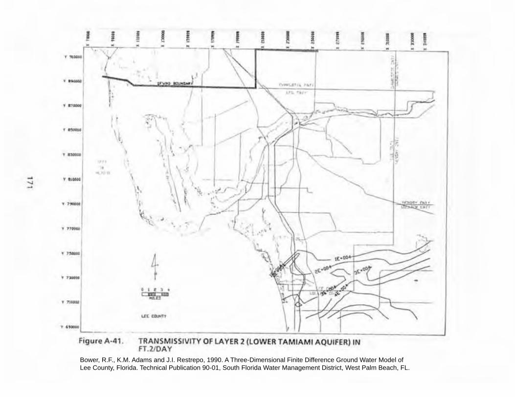
Bower, R.F., K.M. Adams and J.I. Restrepo, 1990. A Three-Dimensional Finite Difference Ground Water Model of
Lee County, Florida. Technical Publication 90-01, South Florida Water Management District, West Palm Beach, FL.

Bower, R.F., K.M. Adams and J.I. Restrepo, 1990. A Three-Dimensional Finite Difference Ground Water Model of
Lee County, Florida. Technical Publication 90-01, South Florida Water Management District, West Palm Beach, FL.
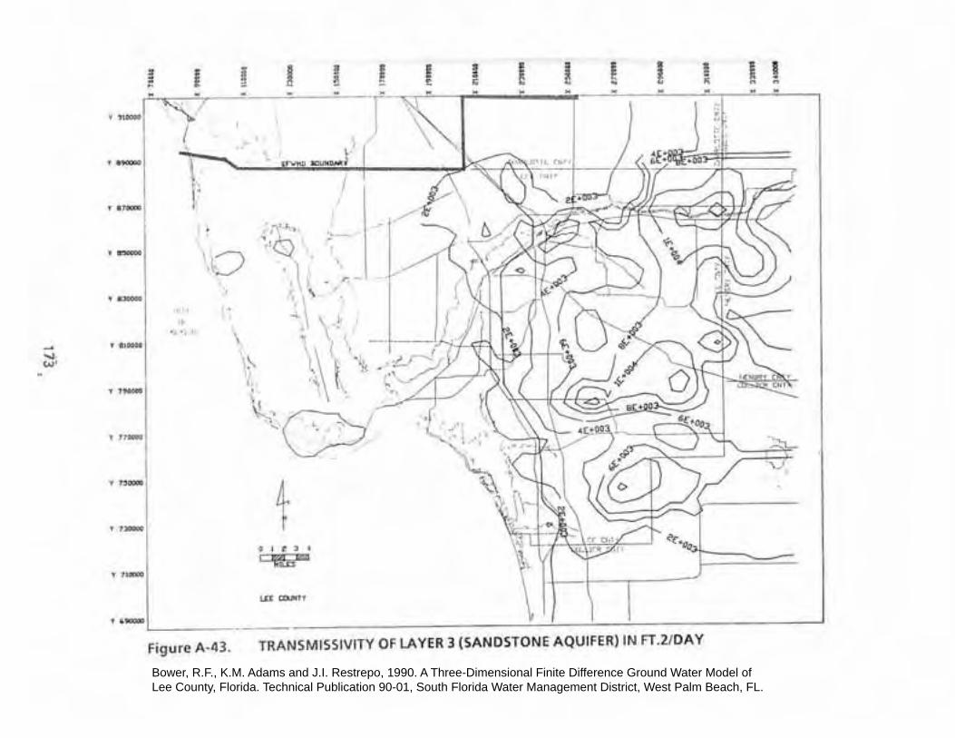
Bower, R.F., K.M. Adams and J.I. Restrepo, 1990. A Three-Dimensional Finite Difference Ground Water Model of
Lee County, Florida. Technical Publication 90-01, South Florida Water Management District, West Palm Beach, FL.
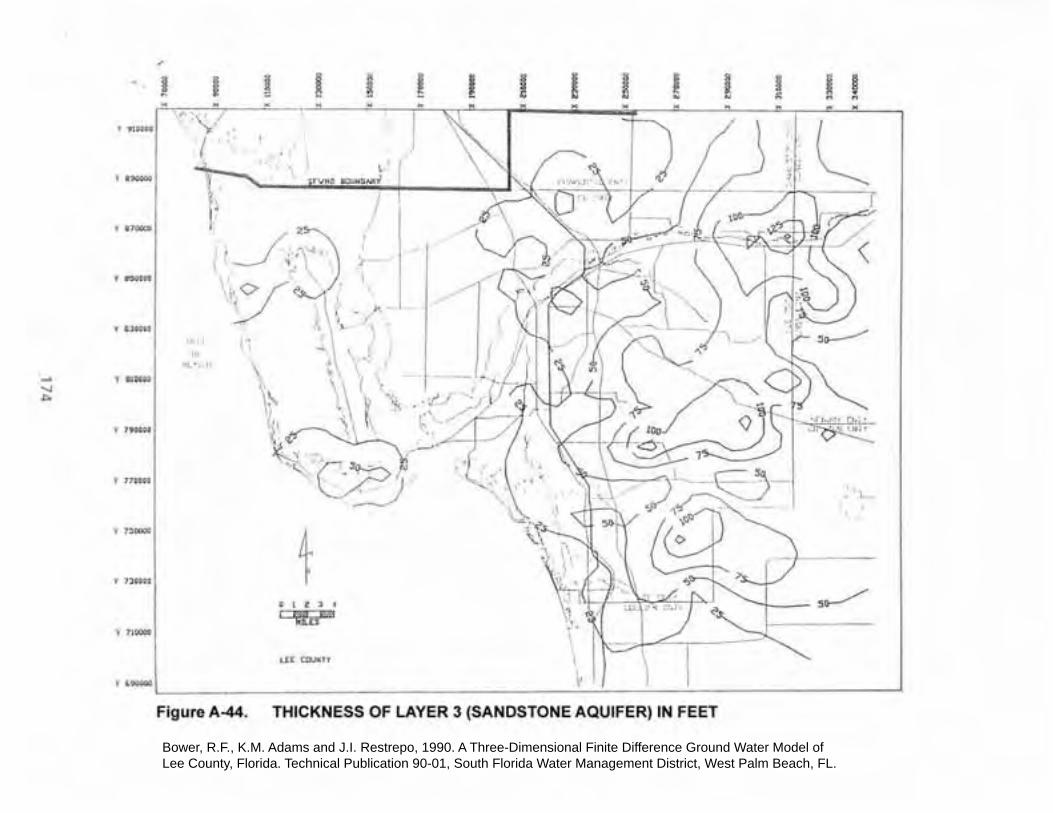
Bower, R.F., K.M. Adams and J.I. Restrepo, 1990. A Three-Dimensional Finite Difference Ground Water Model of
Lee County, Florida. Technical Publication 90-01, South Florida Water Management District, West Palm Beach, FL.
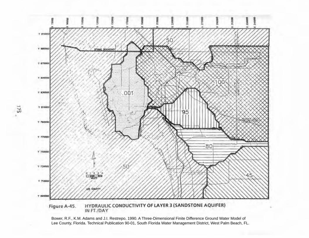
Bower, R.F., K.M. Adams and J.I. Restrepo, 1990. A Three-Dimensional Finite Difference Ground Water Model of
Lee County, Florida. Technical Publication 90-01, South Florida Water Management District, West Palm Beach, FL.

Bower, R.F., K.M. Adams and J.I. Restrepo, 1990. A Three-Dimensional Finite Difference Ground Water Model of
Lee County, Florida. Technical Publication 90-01, South Florida Water Management District, West Palm Beach, FL.
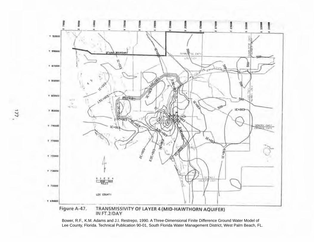
Bower, R.F., K.M. Adams and J.I. Restrepo, 1990. A Three-Dimensional Finite Difference Ground Water Model of
Lee County, Florida. Technical Publication 90-01, South Florida Water Management District, West Palm Beach, FL.
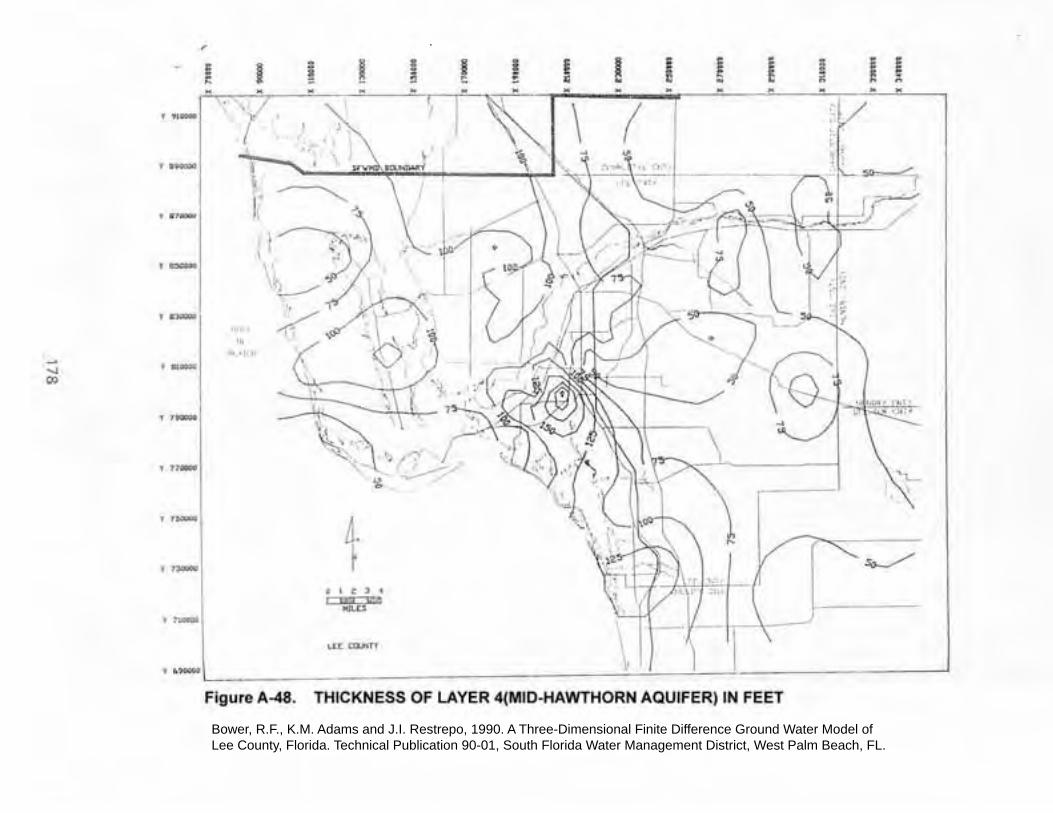
Bower, R.F., K.M. Adams and J.I. Restrepo, 1990. A Three-Dimensional Finite Difference Ground Water Model of
Lee County, Florida. Technical Publication 90-01, South Florida Water Management District, West Palm Beach, FL.

Bower, R.F., K.M. Adams and J.I. Restrepo, 1990. A Three-Dimensional Finite Difference Ground Water Model of
Lee County, Florida. Technical Publication 90-01, South Florida Water Management District, West Palm Beach, FL.

Bower, R.F., K.M. Adams and J.I. Restrepo, 1990. A Three-Dimensional Finite Difference Ground Water Model of
Lee County, Florida. Technical Publication 90-01, South Florida Water Management District, West Palm Beach, FL.

Bower, R.F., K.M. Adams and J.I. Restrepo, 1990. A Three-Dimensional Finite Difference Ground Water Model of
Lee County, Florida. Technical Publication 90-01, South Florida Water Management District, West Palm Beach, FL.
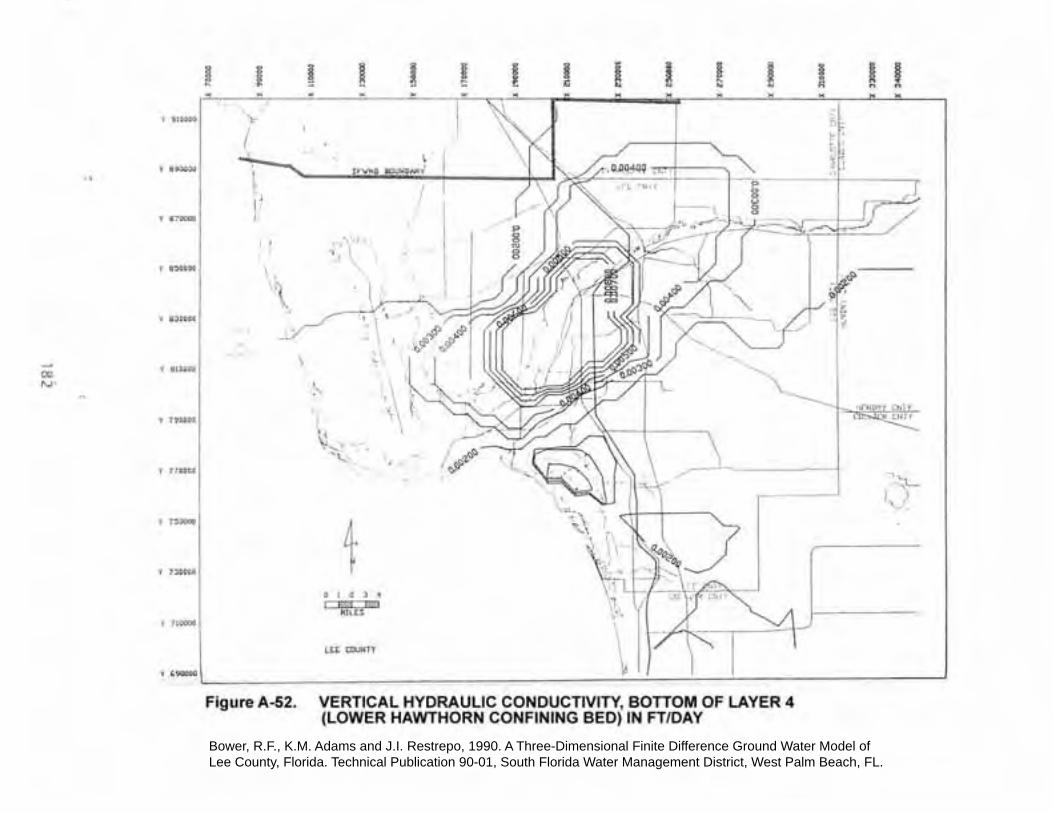
Bower, R.F., K.M. Adams and J.I. Restrepo, 1990. A Three-Dimensional Finite Difference Ground Water Model of
Lee County, Florida. Technical Publication 90-01, South Florida Water Management District, West Palm Beach, FL.
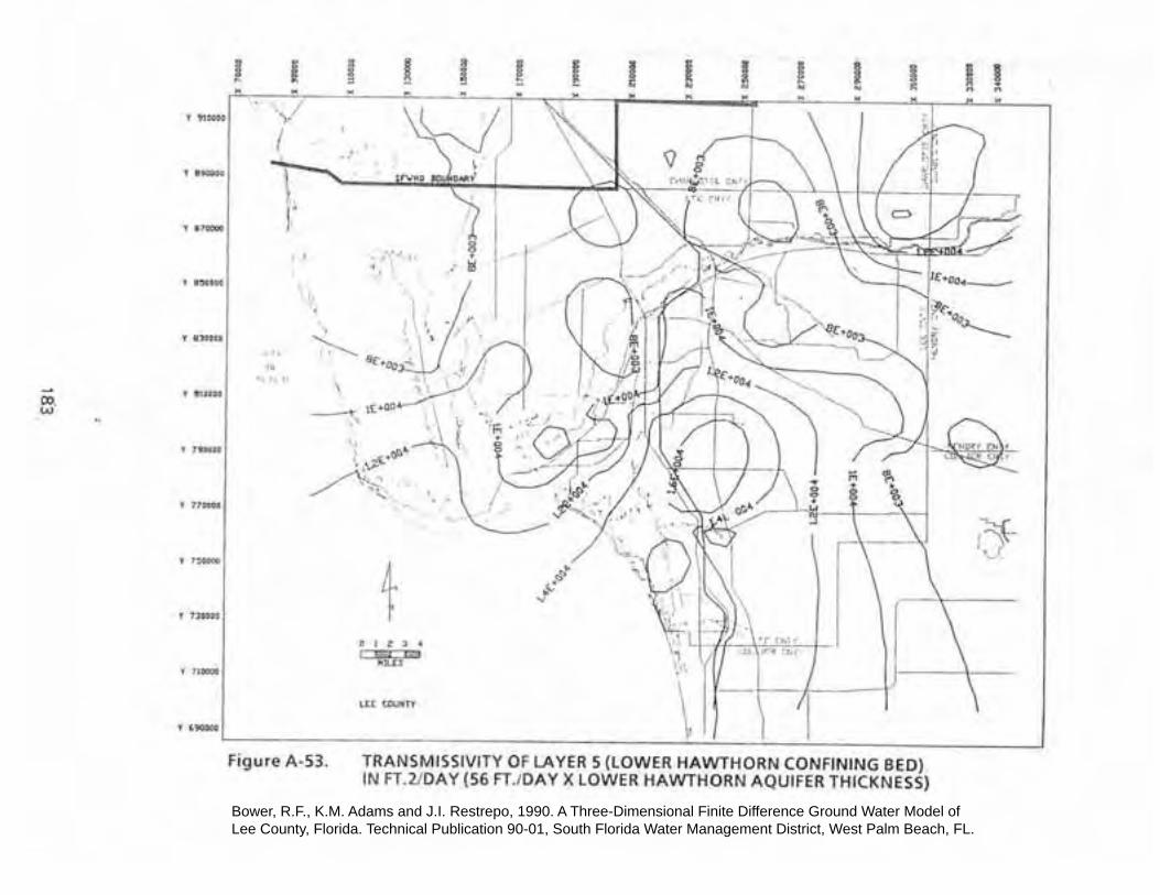
Bower, R.F., K.M. Adams and J.I. Restrepo, 1990. A Three-Dimensional Finite Difference Ground Water Model of
Lee County, Florida. Technical Publication 90-01, South Florida Water Management District, West Palm Beach, FL.
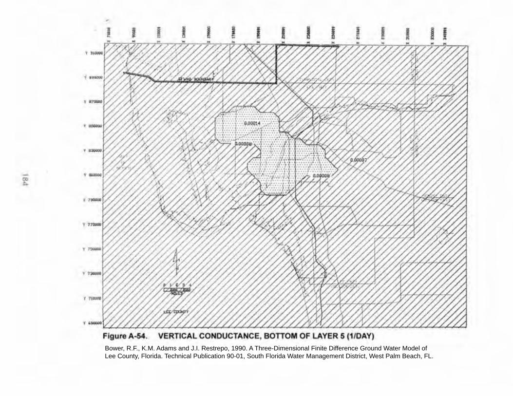
Bower, R.F., K.M. Adams and J.I. Restrepo, 1990. A Three-Dimensional Finite Difference Ground Water Model of
Lee County, Florida. Technical Publication 90-01, South Florida Water Management District, West Palm Beach, FL.
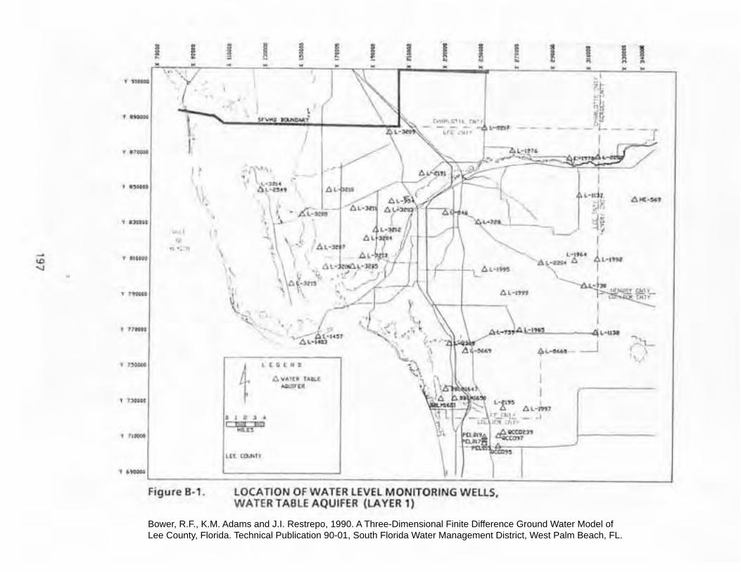
Bower, R.F., K.M. Adams and J.I. Restrepo, 1990. A Three-Dimensional Finite Difference Ground Water Model of
Lee County, Florida. Technical Publication 90-01, South Florida Water Management District, West Palm Beach, FL.
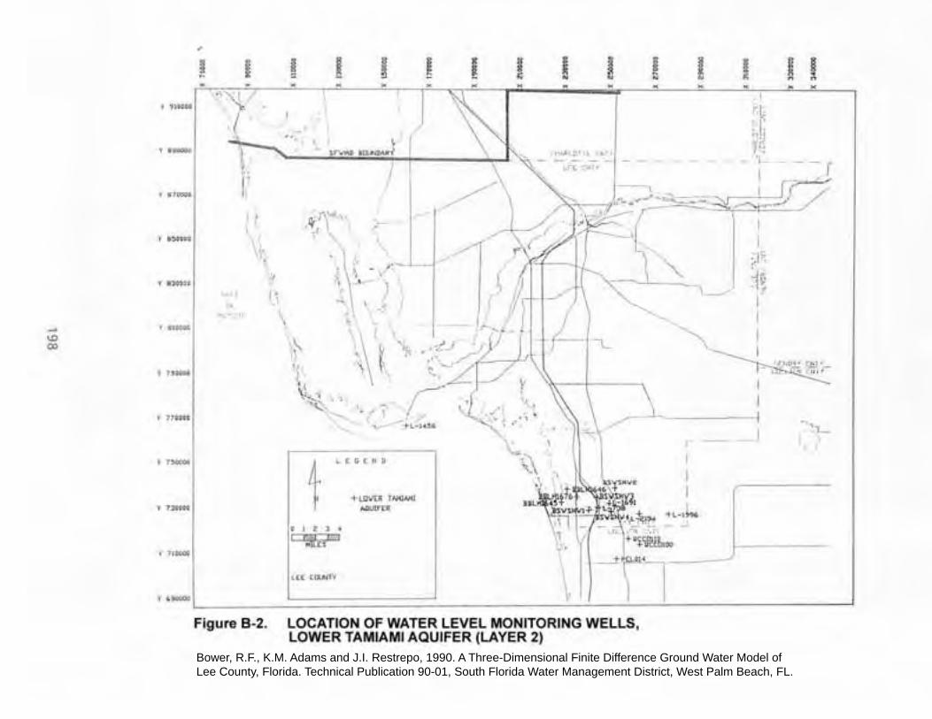
Bower, R.F., K.M. Adams and J.I. Restrepo, 1990. A Three-Dimensional Finite Difference Ground Water Model of
Lee County, Florida. Technical Publication 90-01, South Florida Water Management District, West Palm Beach, FL.

Bower, R.F., K.M. Adams and J.I. Restrepo, 1990. A Three-Dimensional Finite Difference Ground Water Model of
Lee County, Florida. Technical Publication 90-01, South Florida Water Management District, West Palm Beach, FL.
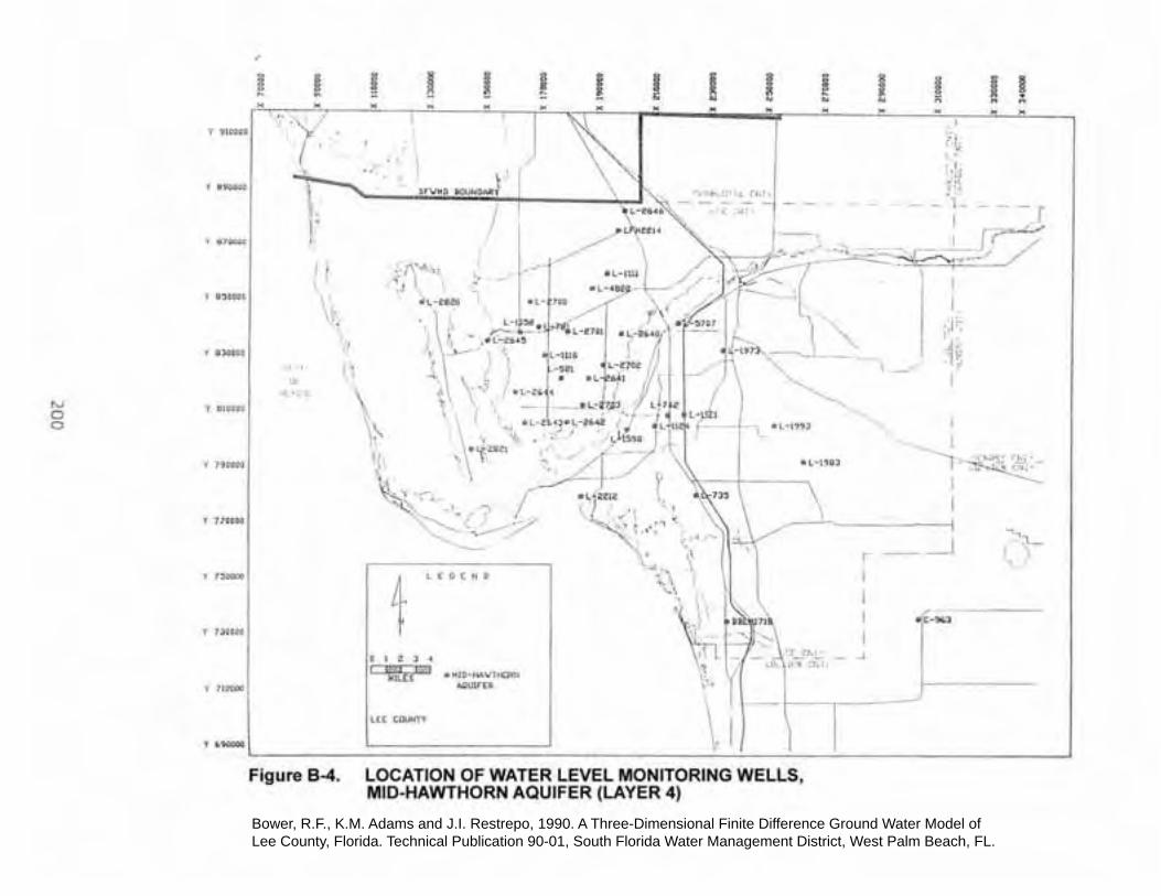
Bower, R.F., K.M. Adams and J.I. Restrepo, 1990. A Three-Dimensional Finite Difference Ground Water Model of
Lee County, Florida. Technical Publication 90-01, South Florida Water Management District, West Palm Beach, FL.
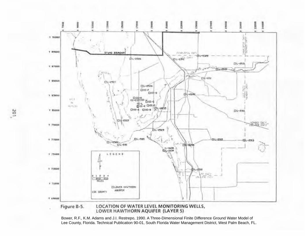
Bower, R.F., K.M. Adams and J.I. Restrepo, 1990. A Three-Dimensional Finite Difference Ground Water Model of
Lee County, Florida. Technical Publication 90-01, South Florida Water Management District, West Palm Beach, FL.