Subcontractors for Tractors: Theory and Evidence on Flexible

Specialization, Supplier Selection, and Contracting�

Tahir Andrabi

Pomona College

tandrabi@pomona.edu

Maitreesh Ghatak

London School of Economics

m.ghatak@lse.ac.uk

Asim Ijaz Khwaja

Harvard University

akhwaja@ksg.harvard.edu

December, 2005.

Abstract

Buyer-Seller networks are pervasive in developing economies yet remain relatively under-studied. Using primary data on contracts between the largest tractor assembler in Pakistanand its suppliers we �nd large variations in prices and quantities across suppliers of the sameproduct. Surprisingly, "tied" suppliers - those that choose higher levels of speci�c investments- receive lower and more unstable orders and lower prices. These results are explained bydeveloping a simple model of �exible specialization under demand uncertainty. A buyer facesmultiple suppliers with heterogeneous types to supply customized parts. Speci�c investmentsraise surplus within the relationship but lower the seller�s �exibility to cater to the outsidemarket. Higher quality suppliers have a greater likelihood of selling outside and so this cost isgreater for them. Therefore even if a buyer typically prefers high types, some low type suppliersmight be kept as marginal suppliers because of their greater willingness to invest more in buyer-speci�c assets. Further empirical examination shows that the more tied suppliers are indeed oflower quality.

1 Introduction

Many industries, particularly in developing countries, are characterized neither as vertically inte-

grated �rms nor as a set of independent buyers and suppliers but as networks. Suppliers provide

specialized inputs to several buyers selling related but di¤erent products and buyers have more than

�This paper is dedicated with great admiration to Pranab Bardhan, whose pioneering work in development eco-nomics combining economic theory and econometric analysis with rich institutional detail has been an inspirationto us all. We thank Abhijit Banerjee, George Baker, Robert Gibbons, Oliver Hart, Alexander Karaivanov, MichaelKremer, Rocco Macchiavello, W. Bentley MacLeod, Kaivan Munshi, Canice Prendergast, Tomas Sjöström, Je¤reyWilliamson, Chris Udry, two anonymous referees, the editor, Mark Rosenzweig and several seminar audiences for help-ful feedback. We are grateful for all the support and information provided by the Lahore University of ManagementSciences and Millat Tractors Ltd. All errors are our own.

1

one supplier for the same input. The resulting investment pattern on the part of suppliers has been

one of �exible specialization and is considered to be an optimal response to demand uncertainty

and costly capacity-building or inventory-holding.1 In such environments, there is considerable

variation in the terms of the contracts faced by a set of sellers who di¤er in terms of how speci�c

their assets are with respect to the main buyer.2

While there is a large literature on the determinants of the boundaries of the �rm that highlights

the importance of relationship-speci�c investments, we know very little about how relationship-

speci�c investments a¤ect contracts when the boundaries of the �rm are given.3 Moreover, the

existing literature treats speci�city as being driven purely by technology. In a network or clus-

ter setting, given that investment is characterized by �exible specialization, the degree of asset

speci�city with respect to any particular buyer is also partly a matter of choice.

In this paper we address these questions both theoretically and empirically. We use primary

data to examine a particular buyer-seller network in Pakistan characterized by high uncertainty,

weak contracting, and costly capacity building. This description �ts the industrial sector of most

developing countries quite well, although the relevance of the framework is not limited to these

countries. Our initial analysis of the network reveals several interesting and somewhat puzzling

facts. We �nd that there is substantial variation in how suppliers are treated - prices di¤er by as

much as 25% and quantities by a factor of three across di¤erent suppliers supplying the same product

in the same year. Upon further examination we �nd that surprisingly, it is the �tied�suppliers (those

that choose higher levels of speci�c investments) that are treated as second preference suppliers,

not only in terms of receiving more unstable and lower orders but lower prices as well.4

We then develop a theoretical model to understand these �ndings. We take the existence of

buyer-seller networks as given and address two main questions: do suppliers of the same product

who di¤er in how speci�c their assets are with respect to the same buyer, receive di¤erent prices

and distribution of orders? What governs the variation in how speci�c a supplier�s assets are in

relation to one buyer?5

1See Piore and Sabel (1984) for a discussion of �exible specialization and Kranton and Minehart (2000) for aformal analysis of when such networks are optimal relative to vertical integration.

2See, for example, Asanuma (1989) for a case study of the Japanese auto-manufacturing industry. In section 2 wereview other studies on this topic.

3See Hart (1995) and Holmström and Roberts (1998) for excellent reviews of the transactions costs and propertyrights literature on the boundaries of the �rm.

4Asanuma (1989) uses the same terms in his case study of the Japanese auto-industry where he reports a similarhierarchy of subcontractors in terms of distribution of orders.

5Kranton and Minehart (2000) analyze the choice between vertical integration and networks of suppliers in modelwith �exible specialization, and the strategic investment incentives of individual �rms that lead to their formation.

2

Our theoretical model has three key ingredients. First, relationship-speci�c investments (as

opposed to general investments) increase the surplus within the relationship but lower the �exibility

of a seller to cater to the outside market. This decrease in �exibility is costly when demand is

uncertain. Second, suppliers are of di¤erent �types� i.e., ex ante qualities. Holding the level of

investment constant, higher types generate a higher level of surplus both within the relationship

and in the outside market. Third, higher types are more likely to �nd a buyer in the outside market.

Because of the �rst and the third features, higher types face a greater marginal cost of undertaking

relation-speci�c investments. Thus for the same level of orders, higher types invest less than lower

types. Therefore the model predicts that even if the assembler prefers high types in general, some

low type vendors might be kept as marginal suppliers because of their greater willingness to invest

in assets speci�c to the buyer, especially when demand is very uncertain.

The model generates further implications that are examined using the primary dataset we

collected on a sample of annual vendor-product speci�c contracts between Millat Tractors Ltd.

(MTL) and its sellers (locally referred to as vendors) for a period of ten years. The MTL data is

attractive for several reasons. First, the focus on a single large buyer ensures that the comparison

between contracts is meaningful. Second, we have detailed contractual outcomes including prices

paid to a supplier for a given product (tractor part) and quantities scheduled every quarter for each

product (henceforth �part�) from the vendor for over a decade. Finally, given the assembler has

multiple vendors supplying the same part, we are able to make cleaner comparisons by contrasting

contracts between two vendors with di¤erent degrees of speci�city but which supply the same part.

Unlike a majority of the empirical literature on relationship-speci�c investments, our comparisons

are therefore not confounded with other e¤ects that may be speci�c to a product yet not related

to relationship-speci�city. Our measure of speci�city is the vendor�s response to what fraction of

its machinery will go to waste if MTL stops buying from it and this measure is con�rmed through

various means such as relating it to a vendor�s production processes.

In addition to the di¤erential treatment results, we �nd that tied vendors indeed have lower

unit production costs, though this makes it even more surprising that they are treated as second

preference vendors. However, cost is not the only consideration of the assembler. It cares a great

deal about timely and defect-free delivery. This suggests that, as in the model, ex ante quality

(type) di¤erences between vendors can explain why MTL does not treat the cheaper tied vendor

Our paper shares with this paper the focus on the advantage of having �exible assets in the presence of demanduncertainty and costliness in maintaining capacity but focuses on a di¤erent and complementary set of questions.

3

as its �rst preference vendor. Indeed, further empirical results show that vendors with greater

asset-speci�city perform worse both in terms of timely and defect-free delivery. In terms of our

theoretical model, low type vendors act as capacity bu¤ers because they are more willing to both

undertake higher levels of speci�c investment and face greater uncertainty.

Our work is related to the theoretical literature on property-rights. The key distinction is that

in our setup only the vendors undertake investments, and so optimal ownership is not the key

question. Also, unlike our model, in this literature speci�c investment is purely technology driven,

and �rm heterogeneity and selection issues are not emphasized.

Our work is closely related to the empirical literature on asset speci�city and how it a¤ects the

nature of contracting.6 In this literature, the e¤ect of asset speci�city is typically shown either

on contract duration (e.g., Joskow, 1987) or on certain contract provisions (e.g., Lyons , 1994 on

the use of formal contracts, Gonzales, Arrunada and Fernandez, 2000 on extent of subcontracting,

Woodru¤, 2002 on the likelihood of vertical integration, and Baker and Hubbard, 2004 on the

pattern of asset ownership). While we too study the e¤ect of asset speci�city on contracts, our

focus is on prices and quantities of orders, and their variability over time and across subcontractors.

More generally, our work is related to the recent empirical literature on contracting where controlling

for unobserved heterogeneity is an important theme (Chiappori and Salanie, 2003).

Finally, we view our work as a contribution to the emerging literature on contracting and

organizational choice in the industrial sector in developing countries. The presence of signi�cant

uncertainty and transactions costs in these economies provide a fertile ground for testing many

predictions of the theory of contracts and organizations. While a rich and growing empirical

literature on contracting and organizational choice exists in the context of agriculture in developing

countries, there is relatively little work in the context of industry (exceptions include Banerjee and

Du�o, 2000, McMillan and Woodru¤, 1999, and Banerjee and Munshi, 2004).7

The plan of the paper is as follows. In section 2 we discuss the key features of the environment

drawing on several case studies on subcontracting in buyer-seller networks from di¤erent parts of

the world. In section 3 we present the theoretical model. In section 4 we examine the case of MTL

and is supplier network and interpret our empirical �ndings in terms of the theoretical model.

Section 5 concludes.6Chiappori and Salanie (2003) and Shelanski and Klein (1995) provide reviews of this literature.7See Mookherjee (1999) for a survey.

4

2 Buyer-Supplier Networks: Key Features & Puzzles

In this section we discuss key features of a particular buyer-seller network in Pakistan.The network

presents some potential puzzles and it is these puzzles that motivate the model developed in the

next section.. We also document that these features hold more generally in other buyer-seller

networks.

Multiplicity:

Our examination of Millat Tractors in Pakistan shows that on average this buyer (assembler)

has 2.3 suppliers for each product. This is not uncommon in such networks as a buyer typically has

multiple suppliers for the same product. Such networks are well documented in the auto industry

particularly in East Asian economies. Chung (1999) mentions that in the Korean automobile indus-

try, �each component was supplied by an average of 3.3 subcontractors in 1998�. Such multiplicity

is also fairly common in developed economies. Milgrom and Roberts (1997), and Forker (1997)

discuss the presence of multiple subcontractors in auto and aerospace industries respectively.

Di¤erential Treatment

The multiple sellers for each product are treated di¤erently by the buyer both in terms of price

obtained and quantity supplied. Such di¤erentials can be quite large. Using the data from MTL

and its suppliers and restricting to cases where two vendors are supplying a given part in the same

year, we �nd that on average one vendor gets a 25% higher price than the other. Doing the same

for quantity supplied shows that on average a vendor is scheduled three times as much as another

vendor supplying the same part in the same year. Similarly, there are di¤erences in the stability of

orders over time. Computing the coe¢ cient of variation (CV) for the quarterly quantity supplied

by vendors for each part shows that the COV ranges from 0.5 to 2 (Table 1). This suggests that

not only is there considerable variation in orders over time, but that this varies across suppliers

with some receiving more stable orders than others.

A broader examination of buyer-seller networks suggests that such di¤erential treatment is

common and often linked to varying supplier quality. Case studies of the Japanese auto industry

(Asanuma,1989) discuss di¤erent tiers of suppliers with ��rst�and �second�preference ones. Sev-

eral case studies document that sellers face di¤erent quantity orders. In Korea, Chung (1999, 2001)

notes that the brunt of the industry�s uneven demand is borne by the smaller suppliers. Most of

the shocks are passed onto the smaller suppliers. Asanuma (1989) notes that American automakers

retained a large number of marginal suppliers and gave them orders only intermittently.

5

Di¤erential supply is particularly relevant in developing economies as they face high demand

uncertainty. Hanson (1995) points out in the Mexican apparel industry that uncertainty associ-

ated with shifting tastes and resulting order changes was important in the rise of subcontracting

networks. Chung (1999) documents how these network relationships were key to the automakers�

response to dealing with the huge uncertainty in the aftermath of the Asian �nancial crisis. In our

examination of the tractor industry in Pakistan, we �nd large yearly �uctuations in tractor sales

in the economy (see Figure 1). Moreover these demand shocks are generally driven by a variety

of idiosyncratic factors. In the Pakistani tractor industry they include unexpected changes in the

interest rates on government loans to farmers to fund tractor purchases, tari¤ and pricing policy

changes, and weather shocks.

The di¤erential treatment often also represents a quality-price trade-o¤. Park, et. al (2001)

give a detailed account of how assemblers in the Korean automotive industry develop elaborate

ratings of the suppliers. Callahan (2000) examines Canadian, Mexican US suppliers in a variety

of industries and notes that while Mexican suppliers were seen as less capable, less cooperative

and lower in quality performance, �nevertheless, the low cost of the Mexican parts made them

cost-e¤ective�.

Relationship-Speci�c Investments

An important feature of MTL�s network is that vendor�s not only report that they incur

relationship-speci�c investments relative to MTL (see section 4 for details) but that the degree

of �tiedness�to MTL varies across vendors, with some reporting no such investments to others re-

porting 100% of their investments tied to MTL. Such investments are fairly typical of buyer-seller

networks and include both physical capital and human capital speci�city. They are thought to lead

to lower costs and improved quality within a relationship, but some loss of �exibility in selling to

other buyers.

Physical capital speci�city appears in the type of machinery used � general-purpose machines

vs. special purpose machines, speci�c tooling dies vs. general purpose assets like presses (Milgrom

and Roberts, 1997) � and the choice of the manufacturing process, e.g., how a machine is �tooled�.

General-purpose equipment has to be �tooled�in certain ways before producing a speci�c part. In

machining, tooling is essentially calibrating a machine so that it produces the �nished part according

to particular speci�cations. In cases where computerized machinery is uncommon such as in the

Pakistani auto industry and the case of MTL�s supplier, such tooling is done manually through

trial and error and involves considerable time and e¤ort, and learning-by-doing. Moreover, since

6

specialized machine manufacturers do not always exist locally in developing economies, at times a

supplier has to develop a specialized machine.8

Human capital speci�city takes the form of relationship-speci�c skills. For MTL�s vendors this

consists of skilled labor embodied in tooling machines to produce particular products, and the

sellers�making their operations and organizational setup compatible to MTL�s. In the Japanese

auto-industry (Asanuma, 1989) - these are skills that the supplier needs to develop to respond

e¢ ciently to the speci�c needs of a particular buyer. Forker (1997) in his aerospace example points

out that less tangible aspects of the relationship such as friendships with purchasing personnel are

all forms of asset speci�city.

An aspect of such relation-speci�c investments that is apparent in case studies but has received

little theoretical attention is that such speci�city is not only driven by technology, but is often a

choice of the supplier and can vary even in producing the same product. We will return to this in

more detail below and incorporate it in the model developed. An example from MTL suppliers is

a multi-drill boring unit. While this machinery can only be used to produce a restricted range of

parts, according to the suppliers we interviewed, it increases accuracy by up to 35% as compared

to using the more general purpose standard single-drill boring units.

How are Tied Suppliers Treated?

The surprising empirical fact is that, along a variety of dimensions, tied suppliers - those that

undertake greater MTL-speci�c investments, receive less favorable treatment by MTL. Table 2

presents the results of examining a variety of outcomes. While we will discuss the data and empirical

results in detail later, we highlight some of these results here because they underline the importance

of understanding the role of investment speci�city and seller heterogeneity.

Columns (1)-(2) show that tied vendors receive a lower level of order. A standard deviation

increase in tiedness is associated with a 5.5%-13.4% drop in the quantity scheduled from the vendor.

While the magnitude is much larger with city and distance controls, the standard errors also

increase.

Columns (3)-(6) examine preferential treatment in terms of the stability of orders given to

vendors. Columns (3)-(4) make use of the time-dimension of the data and ask how MTL passes

on its overall demand variability to its vendors. It does so by computing the elasticity of each

vendor�s scheduled quantity to MTL�s total demand for the given part. It shows that a standard

8For example, one of the sellers we interviewed in the Pakistani auto industry had developed a special press justto create a speci�c part for its main buyer.

7

deviation increase in tiedness is associated with a 3.7 percentage points increase in elasticity (i.e.

from an elasticity of 0.739 to 0.776). Columns (5)-(6) collapse the data to the vendor-part level by

computing the coe¢ cient of variation for the quarterly quantity ordered for each part from a given

vendor over time. The results show that tied vendors are given a more unstable order. A standard

deviation increase in vendor speci�city is associated with a 4.1-5.4% higher coe¢ cient of variation.

Tied vendors face a more �uctuating order i.e. are treated as second preference.

Finally, columns (7)-(8) show that tied vendors also get a lower price. An increase in the measure

of speci�city from 0 to 100 decreases price by 19%; a standard deviation increase in tiedness results

in a 7.9% lower price level.9 These regressions assume that the quality of the lot supplied does

not a¤ect current prices. This is reasonable as the price of each part to be supplied by a vendor is

agreed upon for the entire year before delivery begins.

Why are more dedicated suppliers given less favorable treatment? A priori one would expect

the exact opposite - given that relation-speci�c investments are likely to raise joint surplus, those

suppliers who undertake such investments should be treated more favorably. If they are not, ex ante

they would not choose to be undertake such tied investments. However, this makes an important

assumption that is implicit in the property rights literature - that suppliers are ex ante identical.

An important component of the theoretical model developed is to relax this assumption and allow

for ex ante supplier heterogeneity. Once we recognize that speci�c investments may partly be a

matter of choice, this raises questions regarding the circumstances under which such a choice is

made and whether certain types of suppliers are more likely to choose speci�c investments.

More often than not speci�city choices are a¤ected by the degree of uncertainty in the environ-

ment � stable demand allows the use of dedicated machinery. In contrast,when faced with volatility

in demand (both volume and product mix), suppliers prefer �exible manufacturing processes that

allow them to produce smaller volumes and a larger product mix. German and Roth (1997) dis-

cuss such choices facing automotive engine valve suppliers in Argentina who face a more uncertain

environment than some of their global competitors. These suppliers prefer a process that is more

�exible in that tooling and other �xed costs are lower. So it is easier to shift from one product to

another, but variable costs are higher (e.g., it requires more machining work to achieve the desired

level of precision). The latter type of suppliers choose processes that require a large investment in

9Since we have an unbalanced panel (i.e. for all years the set of parts are not the same) a concern is that ourresults are based only on a comparison of the same part for two vendors across di¤erent years. However, we can checkfor this by allowing for interacted part-year dummy variables. Doing so gives similar results allaying our concern,although, as expected, the standard errors are higher.

8

tooling (i.e., large �xed costs), but are very e¢ cient for producing large volumes.

In addition to uncertainty, suppliers of di¤erent quality may also choose di¤erent levels of speci�c

investments. Forker (1997) points out that while suppliers that are more dependent on their main

customer are cheaper, they often have problems with quality of the components produced. Similarly,

Chung (1999) suggests that in the Korean automobile case it is the lower rung suppliers who are

more dedicated. While such a trade-o¤ is not surprising, what is less apparent is why buyers choose

to have both low and high quality suppliers for the same part rather than just prefer one type. The

model developed, and our subsequent analysis of MTL�s network of suppliers, will explore these

issues further.

3 The Model

3.1 The Environment

The model focuses on the relationship between a single assembler, and its vendors. Everyone is

assumed to be risk-neutral. The assembler is unable to make some parts in-house and needs to

outsource. Vendors produce parts that are then converted into output using some technology by

the assembler. For simplicity, we assume that there is only one part that the assembler needs from

vendors. The production technology involves the assembler using one unit of this part to produce

one unit of the �nal good.

An assembler and a vendor can establish a relationship. This allows the vendor to produce a

customized part to the assembler. Alternatively, the vendor can sell generic parts in the outside

market to any buyer that may knock on its door. Similarly, an assembler can buy generic parts

from the outside market.

The assembler faces uncertain demand: with probability � 2 [0; 1] demand is high (= 2 units)

and with probability 1 � �, demand is low (= 1 unit). Each vendor has the capacity to produce

one unit of the part. Given our speci�cation of demand facing the assembler, this directly implies

that it would need multiple (in the current setting, two) vendors if it wishes to supply the full

amount that is demanded in each state of the world. Therefore, the answer to the question as to

why there are multiple vendors follows directly from the assumption of a particularly simple form

of decreasing returns to scale in our model.

Vendors are of two types, high or low, i.e., �i 2 f�; ��gwhere 1 � �� > � � 0 :Let 4� � ��� �:We

will use the normalization �� + � = 1 which is without loss of generality. We assume that the type

9

of vendor i; �i; is known and observable to all parties, i.e., there is no learning or adverse selection.

There are many vendors of both types in the population. The higher the type of the vendor, the

higher is the surplus within the vendor-assembler relationship. Also, higher type vendors have a

higher expected outside option since they are more versatile and can cater to di¤erent types of

buyers.

A vendor who has established a relationship with the assembler can undertake some relationship-

speci�c investment (henceforth, investment) that enhances the value of trade within the relation-

ship, in the form of higher quality and/or lower costs. Let x 2 [0; 1] denote the level of investment

undertaken by a vendor: We interpret x as the percentage of its total capacity that a vendor keeps

tooled up for producing the customized part to the assembler on demand. The rest of the capacity

is kept �exible so that it can be used to produce generic parts.

The (ex post) joint surplus from trade between the assembler and a vendor of type � is S(x; �) =

a+ b� + x where a > 1; and b > 0: For our analysis it does not make any di¤erence as to whether

the investment improves quality or reduces costs or both. It is easy to modify the above set up

slightly to allow for a separate quality-enhancement and a cost reduction e¤ect. For example, for a

vendor of type � who has undertaken an investment level of x; suppose the unit cost of production

is (x) = 1 � x where 2 (0; 1). Correspondingly, suppose that the (expected) revenue of the

assembler is R(x) = a+ 1 + b� + (1� )x: This ensures that S(x; �) = R(x; �)� (x):

That is, joint surplus is increasing in the quality of the vendor as well as the extent of relationship-

speci�c investment undertaken by it. The (ex ante) cost of undertaking the speci�c investment is

c(x) = 12x2:

The assembler has the option of buying a generic part from the market. In this market the

assembler as well as the vendors are price takers. One unit of a generic part procured from the

outside market yields an expected net surplus of � to the assembler where � 2 (0; 12).

A vendor, whether or not it has established a relationship with the assembler, has the option of

selling generic parts in the outside market. This provides vendors with an outside option in their

dealings with the assembler.

Vendors can earn an exogenously given expected surplus of � per unit of sales in the outside

market where � 2 (0; 12).10 In particular, � is the probability a vendor of type � �nds a buyer in the

market for generic parts. Therefore, the ex ante (i.e., before undertaking any relationship-speci�c

investment) outside option of a vendor is ��. Higher quality vendors face higher expected returns

10 In general, � could depend on �:

10

in the market for generic parts because they can produce a wider range of generic parts and as a

result, are more likely to �nd a prospective buyer.

The ex post outside option faced by a vendor of type � whose investment vis a vis the assembler

is x; is u(x; �) = ��(1 � x): A vendor who has established a relationship with the assembler and

has made some relationship-speci�c investments has a disadvantage in selling the generic part in

the outside market relative to an �unattached�vendor because a part of its capacity is not �exible,

and is less suitable to produce generic parts on demand. In particular,it can produce 1 � x units

of the generic part using the �exible part of its capacity.

As a > 1; it is more e¢ cient for an assembler to establish a relationship with a vendor and

get a customized part (which yields a joint surplus which is at least as large as a per unit) rather

than relying on the outside market for a generic part (which yields a joint surplus of �+� per unit

which is less than 1).

We assume that investment is contractible and is chosen to maximize the expected joint surplus

of the assembler and the vendor. In a previous version of the paper we also analyzed in detail the

case where investment is non-contractible and is subject to a usual hold-up problem. Allowing for

non-contractability does not qualitatively alter our results and in fact makes it more likely that

low types vendors choose higher investment levels even when treated as second preference vendors.

However, for the sake of brevity we will only present the contractible investment case in this paper,

and brie�y mention what happens in the non-contractible case.

Also, in line with the institutional environment where there is a unique assembler and many

vendors, it is assumed that competition between vendors drives their share of the surplus to the

level of their (competitive) outside options. Since x is contractible, the assembler is able to commit

to making a net expected payment of ��x to a vendor of type � who has undertaken investment x

since that ensures an overall expected payo¤ of ��:

Before analyzing the model we should address the issue of vertical integration since this would

matter if investments were non-contractible i.e. why doesn�t the assembler own the asset instead of

the vendors owning it? In the model, we are assuming that the assembler does not undertake any

signi�cant speci�c investments with a speci�c vendor, the ex ante choice of which could be a¤ected

by ex post bargaining. This is justi�ed by the institutional setting. MTL makes tractors based on

blueprints provided by MTL�s foreign partner, Massey-Ferguson and gives the vendor an imported

sample of a relevant part. Any technological support provided is not speci�c to a particular vendor,

but to all vendors that supply that part. Given this, under the non-contractibility case ownership

11

by the assembler will only help to reduce the vendor�s share of ex post surplus, which would dampen

its investment incentives.

3.2 Analysis

Let � � 1 be the demand faced by a vendor from the assembler, to be chosen endogenously. This can

be either a certain demand of � units, or the probability that it is called to supply one whole unit.

We will use the latter interpretation. If x is contractible and the assembler plans to buy � units

of the customized part from a vendor of type �, x will be chosen to maximize ex ante expected

joint surplus between the vendor and the assembler. Under the �rst-best how the assembler and

the vendor split this surplus among themselves has no allocational implications. If demand from

the assembler is not forthcoming (which has probability 1 � �) then a vendor sells generic parts

in the outside market. Therefore, the ex ante expected joint surplus between the vendor and the

assembler is:

s(x) = �S(x; �) + (1� �)u(x; �)� c(x):

which yields the following optimal choice of x:

x�(�; �) = max f� � (1� �)��; 0g : (1)

As � � 1, x�(�; �) < 1: Let �̂(�) be the critical value of � such that x� = 0; i.e., �̂(�) = ��1+�� : Notice

that �̂(�) < 1 and that it is increasing in �. Our �rst result follows immediately upon inspecting

(1):

Proposition 1: (i) The level of investment is increasing in the level of orders.

(ii) The higher is the type of the vendor, the lower is the level of investment for the

same level of order.

(iii) For the range of orders where both types of vendors invest this gap decreases as the

level of orders increases and disappears when the level of orders is 1.

The �rst part of the result follows from the fact that the speci�c investment is useful only when

the asset is used to produce for the assembler, and so the level of speci�c investment is increasing

in the level of orders. The second part follows from the fact that the marginal social return from

relationship-speci�c investment is lower the higher is a vendor�s type. These vendors are more likely

12

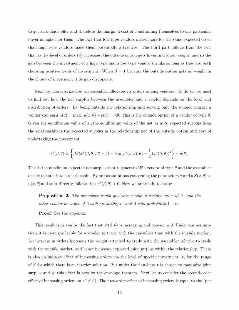
to get an outside o¤er and therefore the marginal cost of constraining themselves to one particular

buyer is higher for them. The fact that low type vendors invest more for the same expected order

than high type vendors make them potentially attractive. The third part follows from the fact

that as the level of orders (�) increases, the outside option gets lower and lower weight, and so the

gap between the investment of a high type and a low type vendor shrinks so long as they are both

choosing positive levels of investment. When � = 1 because the outside option gets no weight in

the choice of investment, this gap disappears.

Next we characterize how an assembler allocates its orders among vendors. To do so, we need

to �nd out how the net surplus between the assembler and a vendor depends on the level and

distribution of orders. By being outside the relationship and serving only the outside market a

vendor can earn u(�) = maxx u(x; �)� c(x) = ��: This is the outside option of a vendor of type �:

Given the equilibrium value of xi; the equilibrium value of the net ex ante expected surplus from

the relationship is the expected surplus in the relationship net of the outside option and cost of

undertaking the investment:

s�(�; �) ���S(x�(�; �); �) + (1� �)u(x�(�; �); �)� 1

2(x�(�; �))2

�� u(�):

This is the maximum expected net surplus that is generated if a vendor of type � and the assembler

decide to enter into a relationship. By our assumptions concerning the parameters a and b S(x; �) >

u(x; �) and so it directly follows that s�(�; �) > 0: Now we are ready to state:

Proposition 2: The assembler would give one vendor a certain order of 1; and the

other vendor an order of 1with probability � and 0 with probability 1� �:

Proof : See the appendix.

This result is driven by the fact that s�(�; �) is increasing and convex in �: Under our assump-

tions it is more pro�table for a vendor to trade with the assembler than with the outside market.

An increase in orders increases the weight attached to trade with the assembler relative to trade

with the outside market, and hence increases expected joint surplus within the relationship. There

is also an indirect e¤ect of increasing orders via the level of speci�c investment, x; for the range

of � for which there is an interior solution. But under the �rst-best x is chosen to maximize joint

surplus and so this e¤ect is zero by the envelope theorem. Next let us consider the second-order

e¤ect of increasing orders on s�(�; �): The �rst-order e¤ect of increasing orders is equal to the (per

13

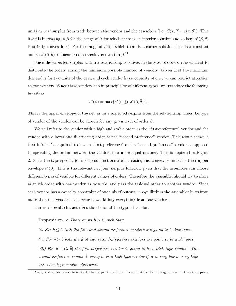
unit) ex post surplus from trade between the vendor and the assembler (i.e., S(x; �)�u(x; �)). This

itself is increasing in � for the range of � for which there is an interior solution and so here s�(�; �)

is strictly convex in �. For the range of � for which there is a corner solution, this is a constant

and so s�(�; �) is linear (and so weakly convex) in �.11

Since the expected surplus within a relationship is convex in the level of orders, it is e¢ cient to

distribute the orders among the minimum possible number of vendors. Given that the maximum

demand is for two units of the part, and each vendor has a capacity of one, we can restrict attention

to two vendors. Since these vendors can in principle be of di¤erent types, we introduce the following

function:

s�(�) = maxfs�(�; �); s�(�; ��)g:

This is the upper envelope of the net ex ante expected surplus from the relationship when the type

of vendor of the vendor can be chosen for any given level of order �:

We will refer to the vendor with a high and stable order as the ��rst-preference�vendor and the

vendor with a lower and �uctuating order as the �second-preference�vendor. This result shows is

that it is in fact optimal to have a ��rst-preference�and a �second-preference�vendor as opposed

to spreading the orders between the vendors in a more equal manner. This is depicted in Figure

2. Since the type speci�c joint surplus functions are increasing and convex, so must be their upper

envelope s�(�): This is the relevant net joint surplus function given that the assembler can choose

di¤erent types of vendors for di¤erent ranges of orders. Therefore the assembler should try to place

as much order with one vendor as possible, and pass the residual order to another vendor. Since

each vendor has a capacity constraint of one unit of output, in equilibrium the assembler buys from

more than one vendor - otherwise it would buy everything from one vendor.

Our next result characterizes the choice of the type of vendor:

Proposition 3: There exists b > � such that:

(i) For b � � both the �rst and second-preference vendors are going to be low types.

(ii) For b > b both the �rst and second-preference vendors are going to be high types.

(iii) For b 2 (�; b] the �rst-preference vendor is going to be a high type vendor. The

second preference vendor is going to be a high type vendor if � is very low or very high

but a low type vendor otherwise.

11Analytically, this property is similar to the pro�t function of a competitive �rm being convex in the output price.

14

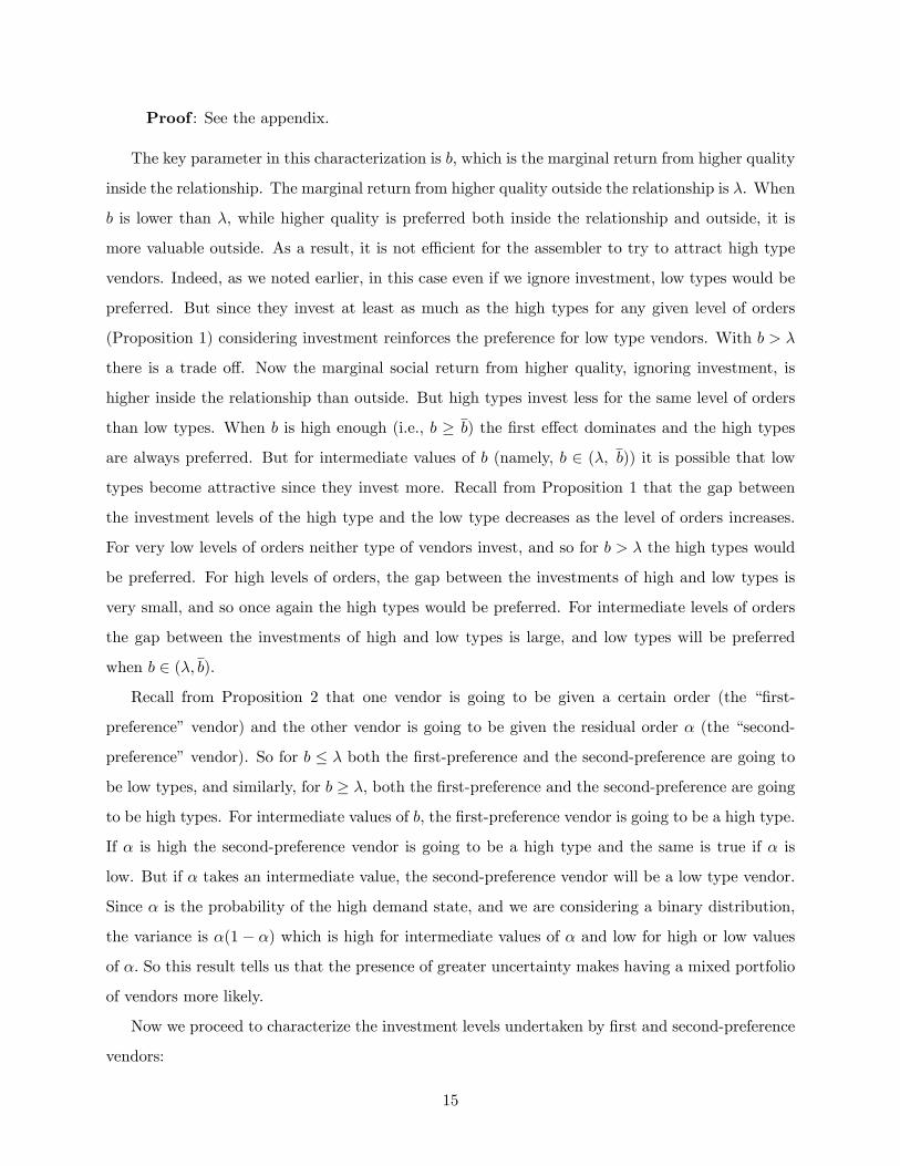
Proof : See the appendix.

The key parameter in this characterization is b; which is the marginal return from higher quality

inside the relationship. The marginal return from higher quality outside the relationship is �. When

b is lower than �, while higher quality is preferred both inside the relationship and outside, it is

more valuable outside. As a result, it is not e¢ cient for the assembler to try to attract high type

vendors. Indeed, as we noted earlier, in this case even if we ignore investment, low types would be

preferred. But since they invest at least as much as the high types for any given level of orders

(Proposition 1) considering investment reinforces the preference for low type vendors. With b > �

there is a trade o¤. Now the marginal social return from higher quality, ignoring investment, is

higher inside the relationship than outside. But high types invest less for the same level of orders

than low types. When b is high enough (i.e., b � b) the �rst e¤ect dominates and the high types

are always preferred. But for intermediate values of b (namely, b 2 (�; b)) it is possible that low

types become attractive since they invest more. Recall from Proposition 1 that the gap between

the investment levels of the high type and the low type decreases as the level of orders increases.

For very low levels of orders neither type of vendors invest, and so for b > � the high types would

be preferred. For high levels of orders, the gap between the investments of high and low types is

very small, and so once again the high types would be preferred. For intermediate levels of orders

the gap between the investments of high and low types is large, and low types will be preferred

when b 2 (�; b).

Recall from Proposition 2 that one vendor is going to be given a certain order (the ��rst-

preference�vendor) and the other vendor is going to be given the residual order � (the �second-

preference�vendor). So for b � � both the �rst-preference and the second-preference are going to

be low types, and similarly, for b � �, both the �rst-preference and the second-preference are going

to be high types. For intermediate values of b; the �rst-preference vendor is going to be a high type.

If � is high the second-preference vendor is going to be a high type and the same is true if � is

low. But if � takes an intermediate value, the second-preference vendor will be a low type vendor.

Since � is the probability of the high demand state, and we are considering a binary distribution,

the variance is �(1 � �) which is high for intermediate values of � and low for high or low values

of �: So this result tells us that the presence of greater uncertainty makes having a mixed portfolio

of vendors more likely.

Now we proceed to characterize the investment levels undertaken by �rst and second-preference

vendors:

15

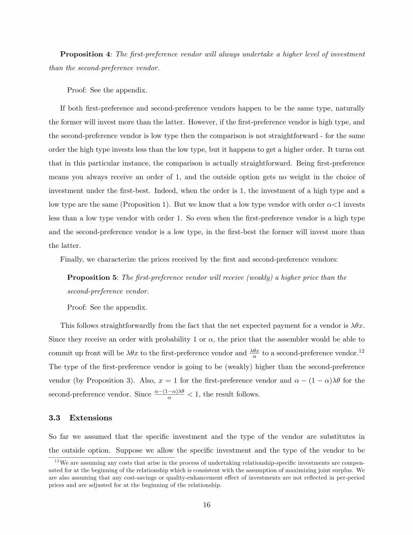
Proposition 4: The �rst-preference vendor will always undertake a higher level of investment

than the second-preference vendor.

Proof: See the appendix.

If both �rst-preference and second-preference vendors happen to be the same type, naturally

the former will invest more than the latter. However, if the �rst-preference vendor is high type, and

the second-preference vendor is low type then the comparison is not straightforward - for the same

order the high type invests less than the low type, but it happens to get a higher order. It turns out

that in this particular instance, the comparison is actually straightforward. Being �rst-preference

means you always receive an order of 1, and the outside option gets no weight in the choice of

investment under the �rst-best. Indeed, when the order is 1, the investment of a high type and a

low type are the same (Proposition 1). But we know that a low type vendor with order �<1 invests

less than a low type vendor with order 1. So even when the �rst-preference vendor is a high type

and the second-preference vendor is a low type, in the �rst-best the former will invest more than

the latter.

Finally, we characterize the prices received by the �rst and second-preference vendors:

Proposition 5: The �rst-preference vendor will receive (weakly) a higher price than the

second-preference vendor.

Proof: See the appendix.

This follows straightforwardly from the fact that the net expected payment for a vendor is ��x:

Since they receive an order with probability 1 or �; the price that the assembler would be able to

commit up front will be ��x to the �rst-preference vendor and ��x� to a second-preference vendor.12

The type of the �rst-preference vendor is going to be (weakly) higher than the second-preference

vendor (by Proposition 3). Also, x = 1 for the �rst-preference vendor and � � (1 � �)�� for the

second-preference vendor. Since ��(1��)��� < 1, the result follows.

3.3 Extensions

So far we assumed that the speci�c investment and the type of the vendor are substitutes in

the outside option. Suppose we allow the speci�c investment and the type of the vendor to be12We are assuming any costs that arise in the process of undertaking relationship-speci�c investments are compen-

sated for at the beginning of the relationship which is consistent with the assumption of maximizing joint surplus. Weare also assuming that any cost-savings or quality-enhancement e¤ect of investments are not re�ected in per-periodprices and are adjusted for at the beginning of the relationship.

16

substitutes or complements within the relationship. Does this qualitatively a¤ect our results? Let

us modify the above model such that S(x; �) = a+ b�+ (1� k�)x where the parameter k allows x

and � to be complements (k < 0) or substitutes (k > 0) as opposed to being independent (k = 0)

which is what we assumed in the benchmark model. This yields the following optimal choice of x:

x�(�; �) = max f� (1� k�)� (1� �)��; 0g :

Clearly, if the investment and the type of the vendor are complements (substitutes) then the

investment advantage of the low types decrease (increase) compared to the above model but the

basic classi�cation of alternative cases remain valid. However, when the investment and the type

of the vendor are substitutes (k > 0) there is an interesting implication for the case where both

high types and low types are chosen in equilibrium. Now the �rst-preference vendor (a high type)

will choose an investment level of 1� k��: However, the second-preference vendor (a low type) will

choose an investment level of � (1� k�) � (1 � �)��: This raises the interesting possibility that

the second-preference vendor might invest more even though it has a lower demand. This will be

the case if the di¤erence between �� and � is large. For example, let �� = 1 and � = 0: Then the

required condition for this becomes (1� �) < k which is possible given our assumptions about the

parameters. However, even if this is the case, so long as the di¤erence between �� and � is large

enough Proposition 5 would continue to hold (����1� k��

�> �� f� (1� k�)� (1� �)��g even if�

1� k���< � (1� k�)� (1� �)�� which is obviously true in the limiting case �� = 1 and � = 0).

Next we consider what happens if x is subject to hold-up problems as in Grossman-Hart-Moore

property-rights framework.13 Let us assume that x is observable but not veri�able. The price for

a vendor is negotiated after the investments are sunk, and the parties are assumed to adopt the

Nash bargaining solution. The assembler bargains with each vendor separately and independently.

If bargaining breaks down with a particular vendor after the investment is undertaken, the vendor

is able to walk out of the relationship and earn its ex post outside option u(x; �).

The assembler can, in principle, �nd another vendor and buy the customized part from it. There

are several costs of doing this. For example, there are costs of screening and training a new vendor

(which we have not modeled), the new vendor would not have had the time to invest, and there

will be some loss of surplus due to delay in delivering to the �nal consumer.14 For simplicity we

13While the choice of a machine (general or special purpose) can in principle be contracted upon, it is harder tocontract on how machines are to be tooled etc. Moreover, in developing country environments where such networksare quite prevalent, contracts are typically incomplete partly due to the high costs of formal contracting.14According to Williamson�s notion of relationship-speci�city, even if one party does not undertake any up front

17

have assumed that these costs are signi�cant and so if bargaining breaks down, the assembler has

to buy a generic part from the outside market which yields a surplus of per unit.15

The gross ex post surplus within the relationship if trade takes place is S(x; �). The vendor�s

share of the ex post surplus from dealing with the assembler per unit of the part conditional on

trade taking place (which can be interpreted as the price) using the standard Nash-bargaining

formula is:

� =S(x; �) + u(x; �)�

2: (2)

The assembler�s share of the ex post surplus in its relationship with the vendor per unit of the part

conditional on trade taking place is:

� =S(x; �)� u(x; �) +

2: (3)

The vendor would choose x to maximize:

�� + (1� �)u(x; �)� c(x):

The vendor�s optimal choice of x is therefore given by:

xSB(�; �) = max

��

2� (1� �

2)��; 0

�(4)

where the superscript SB indicates that this is the optimal second-best allocation. The most

interesting contrast with the case of contractible investment is, now a �rst-preference vendor will

not completely tie itself to the assembler, i.e., even if � = 1, a vendor will keep some capacity �exible

because that enhances its bargaining power by boosting up the outside option. This implies that

the �rst-preference vendor may undertake a lower level of investment than the second-preference

vendor, which will be the case when the �rst-preference vendor is a high-type, and the second-

preference vendor is a low type. Also, so long as the di¤erence between �� and � is large enough

(e.g., �� = 1 and � = 0) Proposition 5 would continue to hold

expenditures at all, his ex ante relationship-speci�c investment could just be the choice of a partner or a standard oranything else that limits his later options.15This ex post bargaining power of the vendor is perfectly consistent with ex ante competition among vendors to

be able to trade with the assembler, and is a consequence of relationship speci�city.

18

3.4 Discussion and Empirical Implications

The theoretical analysis above establishes how one obtains equilibrium order patterns that involve

giving relatively stable (certain in our model) and higher orders to one vendor and variable and

lower orders to another vendor. The observed pattern of assemblers having �rst-preference and

second-preference vendors emerge endogenously in our model with heterogeneous types of vendors,

and optimally chosen investment levels. In addition, Proposition 3 shows that the �rst-preference

vendor is going to be (weakly) higher quality than the second-preference vendor. We then show that

the �rst-preference undertakes a higher level of investment as compared to the second-preference

vendor in the basic model. However, in the extension section we showed that if x and � are strong

substitutes within the relationship or if there is a hold-up problem, the second preference vendor

may undertake a higher level of investment.

Since we do not directly observe type �, the empirical implications of the above analysis involve

a set of predictions about investment x� (which is observed) and the following: level and variability

of orders, unit costs, price per unit, and quality (or performance).16 Without taking into account

selection e¤ects, we would expect x� to be positively related to the level of orders, price per unit, and

quality (or performance), and negatively related to variability of orders and unit costs. However,

once we recognize the selection e¤ects, some of these conclusions will have to modi�ed, as our

analysis shows above.

4 Empirical Evidence

The motivating empirical results presented in section 2 showed that not only is there supplier multi-

plicity and di¤erential treatment of MTL suppliers, but that somewhat surprisingly, suppliers that

choose to invest speci�cally for MTL receive less favorable treatment in terms of price and quantity

levels and the variability of orders. The model developed above presented a theoretical framework

which shows that this puzzle can be resolved once we allow for ex ante supplier heterogeneity. It

shows that in equilibrium it is possible that the lower quality suppliers are willing to choose greater

levels of relationship-speci�c investments and that MTL buys from both the low and high quality

suppliers. While the data is not detailed enough to uncover the structural parameters in the model,

16While we do not explicitly talk about unit costs, as we mention in the model set up, a part of the bene�t ofinvestment could be in reducing unit costs. So if unit cost of production is (x) = 1� x then it would be decreasingin x: Similarly, if there is a separate quality enhancement component of investment, we would expect that to beincreasing in x:

19

and to test the parameters values under which di¤erent model cases occur, we can examine the

empirical implications suggested by the model in order to reconcile why tied vendors are second

preference - speci�cally, that tied vendors are of lower quality/type.

4.1 Data

MTL is licensed to produce two models of Massey-Ferguson tractors and does so by mostly out-

sourcing (only 7 out of the 500 tractor parts are manufactured in-house 17) to a rich and stable

base of 200 local vendors with very little turnover in these vendors. The vendors are selected by

MTL after a rigorous examination of their technological capability and MTL is therefore aware of

each vendor�s strengths and weaknesses i.e. vendor type, as in the model above, is known to MTL.

MTL mostly has multiple vendors for each part, while each vendor typically also supplies to sev-

eral buyers, including other tractor assemblers, the market for replacement parts, and automobile

manufacturers.

Once a vendor is approved to supply a particular product - a tractor part - MTL negotiates a

price for the part and issues a tentative quantity order. While the price agreed upon for the period

of the contract (generally a year) is binding for both parties, there is no commitment on quantity.18

The supply schedule is issued each quarter and is determined by demand conditions. As such, in

our empirical analysis we will focus not only on the negotiated price but also on both the quantity

scheduled each quarter and the quantity that the vendor delivers.

There are two aspects of a vendor�s supply that MTL is concerned about - part and delivery

quality. A key quality issue is a part failing to meet measurement speci�cations. The incorrect

measurements result either from vendor error or using equipment beyond their acceptable lifetime.

As such MTL has elaborate part-quality control mechanisms ranging from tests of random samples

for each batch supplied to assembly-line �tting and �eld problems. Timely delivery of the quantity

ordered is the other major concern for MTL. This is especially important since MTL requires all

parts to assemble its �nal product and so, inventories aside, a single vendor may hold up MTL�s

production line if it delays delivery.

An important feature is the high degree of uncertainty in yearly sales the tractor industry in

17A medium sized tractor assembled by MTL requires around 900 components, of which 400 are imported. Acomponent normally comprises of several parts (e.g., a set of bolts required for one wheel is treated as a componentby MTL). The vast majority of local vendors produce metalwork parts. In 1994, 54% of the total value of partsprocured by MTL was from local vendors. See Amir, Isert and Khan (1995).18Price renegotiations within the contract period happen rarely unless there is some large unexpected change in

input prices (e.g., a hike in raw steel prices).

20

Pakistan faces. Figure 1 shows this high degree of volatility during 1989-99. There are several

reasons for this uncertainty, ranging from erratic government policy (concerning the �nancing of

tractor purchases by government banks, imports, taxes) to demand �uctuations driven by unstable

agricultural output growth.

We employ two data sources. The primary dataset consists of part-speci�c contracts between

MTL and its vendors during 1989-99 and additional part level information from the archives at

MTL. The data provides negotiated price and quarterly quantity scheduled and received by vendor

for each part. The parts are representative, ranging from low priced simple products such as tractor

clips (Rs. 0.2) to high priced complex products such as a transmission case (Rs. 5306). This data-

set is merged with a survey of the automobile industry vendors conducted by the Lahore University

of Management Sciences (LUMS) in 1997 to construct vendor attributes. This leaves us with a

sample of 28 MTL vendors.

We further restrict our analysis to parts for which MTL buys from more than one of the 28

vendors in our sample. This restriction allows us to address the main question of interest, namely

how prices and quantities vary across vendors supplying the same part. Otherwise we would be

comparing vendors that supply di¤erent products, and even though we allow for a part-speci�c

intercept, we would not be able to separate out the e¤ect of a �rm�s characteristics from choices

such as its degree of relationship-speci�city. The drawback is the smaller sample size � we are

left with 19 of the 28 vendors supplying 39 di¤erent parts � produces potentially higher standard

errors.

Table 1 gives the de�nitions and summary statistics for the main variables used. The primary

outcomes of interest are the annual price for each part and vendor, and the quantity ordered and

subsequently received from each vendor. Note that we do not have any direct measure of the type

of the vendor (i.e. � in the model). As such the primary explanatory variable is the degree of

relationship-speci�c investments (x in the model) undertaken by the vendor. This is measured as

the percentage of the vendor�s physical assets/equipment that would become idle i.e. would have

to be scrapped if MTL stopped buying from it.19

Given the importance of speci�city, it is important that our measure capture the degree of

speci�c investments and not an omitted factor such as a vendor�s dependence on MTL or con�dence

in its own abilities. We provide several checks for this. First, using MTL engineers ranking of

19Alternately this measure can be thought of as the level of quasi-rents (see Williamson 1985) generated by thespeci�c-investment. Andrabi, Ghatak and Khwaja (2004) consider this alternate interpretation and �nd that it leadsto a similar but more involved explanation of the empirical �ndings.

21

technological processes, we show that our measure is higher for processes that are more likely to

require dedicated investments. Vendors involved in machining and forging, both high-speci�city

processes, declared speci�city measures of 62% and 66% whereas those that only did casting, a

low-speci�city process, had much lower speci�city measures. Second, we check for an obvious

misinterpretation with �sales reliance�on MTL and �nd that a vendor�s percentage sales to MTL

and its declared speci�city are not correlated, suggesting that this misinterpretation is not an

issue.20

4.2 Empirical Speci�cation

Our data restriction to parts with multiple sample vendors allows us to use part and time �xed

e¤ects to contrast contractual outcomes for two di¤erent vendors supplying the same part in the

same year. This is the tightest restriction we can apply, though at the cost of reducing sample size.

Part �xed e¤ects control for potentially important and confounding aspects speci�c to the part (such

as its technological nature, how critical it is, the number of vendors supplying it provided that this

does not change over the sample period etc.) and time �xed e¤ects control for common period-

speci�c shocks such as in�ation, demand, and government policy changes. We will be estimating

equations of the form:

Cijt = �i + � t +Xj

�jXj + error: (5)

Cijt = (level of) contractual feature/outcome for part i, vendor j; in period (year or quarter)

t; Xj = time-invariant vendor characteristic; �i = part-speci�c intercept and � t = period-speci�c

(year/quarter) intercept.

One caveat is that this speci�cation treats vendor characteristics as time invariant. At a practical

level this is dictated by the fact that we have information on some vendor characteristics such as

speci�city for only one year. However, we are not unduly concerned since these attributes do

not change substantially over the short time period under study (11 years, with 96% of the data

coming from the period 1993-1999) as supported in cases where we have another year of vendor

20One might expect that a vendor that has less dedicated assets to MTL will have fewer sales to MTL and viceversa. Neither relation is necessarily true. First, a vendor could be making all its sales to MTL but it could be usinggeneric machinery to produce the parts and as such have low speci�city. As a result, if MTL stops buying from it, itcould switch to another buyer. Indeed, in our �eld interviews we found a vendor involved in machining that makesall its sales to MTL, but since it uses lathe machines that can easily be switched to produce parts for another buyer,it reported a speci�city of zero. Now consider the converse. It would seem that a vendor that has a high speci�cityshould be making most of its sales to MTL. However, this is not necessarily the case. A vendor could be very tied toMTL but could still be making most of its sales for the part it produces for MTL in the replacement market insteadof directly to MTL.

22

characteristics (correlations between vendor size observations in 1985, 1990 and 1995 are all above

0.95 and highly signi�cant). Moreover, even if they do change, as long as they change uniformly

i.e. vendors do not keep switching rank there is unlikely to be any systematic bias in our results.

The functional form used was dictated by the particular dependent variable being considered.

For regressions in which the dependent variable is price/cost, we use a log-linear speci�cation be-

cause prices/costs across di¤erent products tend to have a fairly skewed distribution that resembles

a log-normal rather than normal distribution. In contrast, in speci�cations where the dependent

variable is quantity, the distribution is much less skewed. While we could run these regressions as

linear, we choose a log-log speci�cation both because we feel it is more appropriate and because the

coe¢ cients have natural elasticity interpretations (the two exceptions to this are two tables that

have quantity coe¢ cient of variation and percentage rejections as the dependent variables �there

we stick with the simpler linear level speci�cation). However, we should note that our results are

qualitatively robust to using only one (linear) speci�cation form.

While we are primarily interested in vendor speci�city, we also include other vendor attributes

as robustness checks. For example, controlling for �rm age21 and size allows us to take into account

learning-by-doing e¤ects or economies of scale a¤ects.22 For all regression tables, the �rst speci�-

cation reports the result with a smaller set of basic controls (speci�city, age, size) and the second

adds more controls (the distance from MTL, a city dummy). The estimated coe¢ cients below are

from the latter unless noted otherwise.

4.3 Results

We have already discussed results in Table 2 that show tied suppliers are treated less favorably by

MTL. To recap, (i) Tied vendors receive lower orders- a standard deviation increase in tiedness is

associated with a 5.5%-13.4% drop in the quantity scheduled from the vendor (Table 2, columns

(1)-(2)); (ii).Tied vendors face more unstable orders (Table 2, columns (3)-(6) - a standard deviation

21We also have data on years of relationship. It is highly correlated with the age of a vendor and our results aresimilar if we use this variable instead of age.22A concern is whether �rm size belongs as a regressor. While omitting it does not qualitatively a¤ect our results,

we prefer to keep it in for the following reasons: First, these �rms are not only serving one buyer. While MTLis often their main buyer, it is not the exclusive one, with suppliers making sales to other assemblers and thereplacement market. As such vendor size, measured by number of employees, while a function of quantity sold tothe main assembler, is not its only determinant (in fact bigger suppliers do not sell proportionately more to theirmain assembler i.e. percentage sales to main assembler is not signi�cantly correlated with �rm size). Second, strictlyspeaking, our model compares two vendors with the same capacity constraints, being treated di¤erentially. To theextent that vendor size is a proxy for production capacity, controlling for it is more along the lines of the theoreticalframework.

23

increase in tiedness is associated with a 4.1-5.4% higher coe¢ cient of variation and a 3.7 percentage

points increase in elasticity of each vendor�s scheduled quantity to MTL�s total demand for the

given part; (iii) Tied vendors get a lower price. A standard deviation increase in tiedness results in

a 7.9% lower price level (Table 2, columns (7)-(8)). We now turn to some further empirical result

suggested by the model.

One of the important assumptions in the model is that relationship-speci�c investments not

only exist but generate surplus. One way to see whether this assumption has empirical merit is to

check whether investments in relationship-speci�c assets lead to greater surplus in terms of lower

production costs. Fortunately, for a sub-sample of parts we have internal cost estimates generated

by MTL engineers. These estimates calculate how much it costs a particular vendor to produce

the given part. Since MTL engineers are intimately familiar with the machines and production

processes used by each vendor, these cost estimates vary for the same part across di¤erent vendors

and provides a way for us to test whether vendors with lower speci�city have lower production costs.

Table 3 shows that this is indeed the case: An increase in speci�city from 0 to 100% decreases level

costs by 15%: Alternatively, a standard deviation increase in speci�city lowers costs by 6.6%.23

Production costs also fall in the age and size of the vendor suggesting learning by doing and scale

economies and lending further credibility to the cost results.

Now lets turn to reconciling the apparently puzzling results in table 2 - that tied vendors are

treated as second preference vendors when, if anything, MTL should prefer and hence better treat

vendors that choose to invest in speci�c assets. Recall that, as illustrated in the model, once we

admit there is vendor heterogeneity, the choice of how much speci�c-investments to make may also

re�ect a vendor�s type i.e. all else being equal, low type vendors choose to be more tied to MTL.

Under high �nal product uncertainty (which MTL faces - recall Figure 1) we can also get that

low type vendors may choose a higher level of speci�c-investments despite getting a lower order

(Propositions 3 and 5). While we do not have direct measures of vendor type, we can check whether

this explanation is consistent with the empirical evidence by looking at the �nal quality of the tied

vendors.24 Since, all else being equal, investing in more dedicated assets should raise quality, if

the �nal quality of tied vendors is in fact lower, this lends strong support that vendors of lower

23 In general, the magnitude of the e¤ect is calculated from a one standard deviation increase in speci�city startingat 0 speci�city. The percentage change is then evaluated at mean of the dependent variable.24 In general, it is not easy to separate the e¤ects of vendor type from its choice of speci�ty without a direct measure

of the former. Using vendor �xed e¤ects is unlikely to help since both quality and asset-speci�city are likely to betime-invariant. Having an instrument for vendor type may not solve the problem since, as the model shows, thiswould also a¤ect the choice of speci�city.

24

type (i.e. initial quality) are more likely to choose speci�c-investments and is able to reconcile our

previous empirical results in light of the model. Our results below show that this is indeed the case.

Table 4 shows that tied vendors�supply is of lower quality. A standard deviation increase in

tiedness is associated with a 43.6% increase in the proportion of a vendor�s order that is rejected

because it fails to meet MTL�s quality standards. However it should be noted that this proportion

is generally quite low, with a mean value of 1% (the increase is from 1% to 1.43%) suggesting that

in general MTL�s quality control is fairly e¤ective.

MTL is also concerned about delivery performance i.e. does a vendor deliver the amount that

is ordered and is this delivery on time. We can examine this question since, in addition to the

quantity ordered from the vendor, we also have the quantity that the vendor delivered in response

to the order. Tables 5-6 take a closer look at delivery performance and reveal that tied vendors

perform worse on this dimension as well.

Columns (1)-(2) in Table 5 show that a tied vendor is less responsive to the quantity MTL

orders from it. A standard deviation increase in tiedness is associated with a 8.7 percentage points

decrease (from 0.474 to 0.387) in elasticity of the quantity a vendor delivers with respect to the

quantity that MTL asked of it (column (2)). A possible concern could be that since tied vendors

are given a more unstable order this is to be expected. However, as Columns (3)-(4) con�rm, tied

vendors are also less responsive to MTL�s overall demand for a given part.

Table 6 provides further evidence for the poorer delivery performance of tied vendors. It shows

that tied vendors are more likely to both undersupply (columns (1)-(2)) and oversupply (columns

(3)-(4)) quantity i.e. the quantity received is less/more than what MTL ordered. Column (2) shows

that a standard deviation increase in tiedness is associated with a 24% increase in the quantity that

is undersupplied by the vendor. Column (3) shows that a standard deviation increase in speci�city

is associated with a 10% increase in quantity oversupplied, although this result is not robust to city

and distance controls. A point worth clarifying is that while under-supplying is clearly a problem

for MTL, it is not obvious why over-supply is a problem. Discussions with MTL revealed that due

to inventory costs and management reasons MTL disliked over-supply.25 From the vendors�point

of view, for parts with signi�cant �xed production costs (e.g., tooling a machine), batch production

is preferred and so the vendor may bring in a larger order than they are asked to in a given month.

Also recall that due to high �nal demand uncertainty MTL does not commit on annual quantity

25 It is costly to hold additional parts not only because of direct investory costs but also, since these parts cannotbe utlized by themsleves, an over-supplied part complicates the inventory management problem of �guring out howto alter future orders for both the over-supplied and other tractor parts.

25

orders, but issues quarterly orders which often change from month to month. Thus over-supply

can also be due to MTL asking the vendor to supply less than what it did in the previous quarter.

A vendor that is not able to do so, is performing poorly from MTL�s perspective.

While Tables 4-6 show that tied vendors have lower quality in terms of part rejections and

delivery performance, ideally one would have liked to test whether vendors of a lower type i.e.

ex ante quality choose greater relationship-speci�c investments. Unfortunately the data does not

provide any obvious measure of ex ante vendor quality. One could imagine using age of vendor as

one such measure but in a regression of speci�city on age and other characteristics, age and vendor

size do not seem to matter. What does matter is city - vendors in Karachi have higher speci�city

levels. Similarly, we asked the assembler to rate its vendors and while this measure is potentially

driven by ex post rather than ex ante quality measures and fairly subjective (which is why we prefer

not to use it in our main empirical speci�cations), it is the case that higher quality vendors have

lower speci�city levels.

4.4 Alternative Explanations

The MTL case reveals that vendors choosing greater speci�c investments are treated as second

preference. This result can be explained by the theoretical model which shows low type vendors

may be more willing to undertake speci�c investments. Moreover, as the model illustrates, under

demand uncertainty MTL deals with such low types not only because they invest in speci�c-assets,

but because they are willing to act as capacity bu¤ers i.e. MTL passes on more of its shock to

them. Thus in equilibrium we see MTL buying from both types - high quality but less tied and low

quality but more tied vendors. While the empirical case is not meant as a test of the model, it is

nevertheless worth asking whether there are simpler alternative explanations of the MTL �ndings.

Can an explanation be provided without relying on the role of speci�c investments? Since

tied vendors are willing to be treated as marginal vendors, an explanation would still require that

they are of lower ex ante quality i.e. lower type. We have already addressed a concern that our

speci�city measure may not re�ect speci�c-investments but that lower type vendors report a higher

measure because their outside options are worse. The fact that our measure is correlated with

the speci�city expected under di¤erent manufacturing processes used by vendors and that it is not

correlated to their sales to MTL, suggests that this concern is unwarranted. Even if this were true,

a further argument would be needed to explain why MTL deals with both high and low quality

vendors. Vendor shortage or type unobservability is unlikely since MTL carefully selects its pool

26

of 200 active vendors out of a population of over 2,000 vendors. Moreover, even for its existing

high quality vendors, our data shows that neither are their sales exclusively to MTL, nor are they

producing near plant capacity,26 further suggesting that MTL chooses not to have them supply

more.27

Does one require that speci�c investments hurt outside options? What if we only assume this

investment and vendor type are substitutes within the relationship? In this case while high types

invest less than low types as before, the investment gap between the high and low types is now

decreasing in the level of orders. This means if low types are hired at all, they are more likely to

be used as �rst-preference vendors which is inconsistent with our empirical �ndings.

Finally, what if there is no ex ante vendor heterogeneity (i.e. only one vendor type) but being

tied has the exact opposite e¤ect from what we have assumed i.e. it lowers ex post quality? This

seems implausible both because it is contrary to the literature and because our data suggests there

are direct gains from being tied in terms of lower production costs. Moreover, if being tied did

lead to a worsening of a vendor�s quality, why would it ever choose to be tied, especially since it

is treated worse in terms of prices and quantities ordered if it becomes tied. These is no evidence

that MTL provides any other assistance to tied vendors such as loans etc.28

5 Conclusion

The relationship between a tractor assembling �rm in Pakistan and its subcontractors o¤ers impor-

tant insights about contracting and asset speci�city within a buyer-supplier network. The presence

of demand uncertainty makes undertaking relationship-speci�c investments costly on the part of

suppliers. This cost is likely to be more, the more able and versatile the supplier. Therefore there

is a chance for low quality suppliers to survive because of their greater willingness to undertake

speci�c investments and this may explain why there continues to be vendor heterogeneity and dif-

ferential treatment in buyer-seller networks. In the case of MTL tractors, this explains the puzzle

26While most vendors produce below capacity, a regression (not shown) of capacity utlization on vendor speci�cityshows that tied vendors are signi�cantly more likely to have lower capacity utlization. A standard deviation increasein tiedness is associated with 21 percentage points lower plant capacity utlization.27Alternatively, one could make restrictive assumptions on the demand function facing MTL such that it demands

both low and high quality parts from its vendors. For instance, MTL might be selling two di¤erent qualities of thesame tractor with more variable demand from customers who value quality less. However, this seems quite unlikelysince MTL can only sell tractors at uniform prices predetermined by the government and it is implausible that itcan consistently �fool� less quality conscious consumers to buy inferior tractors at the same price. Also, there is noevidence that MTL employs any non-price mechanisms of discriminating among di¤erent types of customers.28The data shows MTL provides little �nancial support to vendors and there is no correlation between �nancial

assistance received and the extent of speci�city.

27

we observe that the buyer treats suppliers with greater asset-speci�city as marginal suppliers even

though they are cheaper.

Our work also suggests that asset speci�city should not always be viewed as purely technology-

driven, which has been the dominant view in the organizations literature, but may partly be a

matter of choice. If so, one has to be careful in interpreting the e¤ect of asset-speci�city on

contractual and performance outcomes since such e¤ects may also re�ect heterogeneity across the

�rms that choose di¤erent asset-speci�city levels.

References

[1] Amir, I., K. Isert, and S. Khan (1995): �Note on the Local Suppliers to the Tractor Industry

in Pakistan�, Mimeo. Lahore University of Management Sciences, Lahore, Pakistan.

[2] Andrabi, T; M. Ghatak and A. I. Khwaja (2004): �Subcontractors for Tractors: Theory and

Evidence on Flexible Specialization, Supplier Selection, and Contracting� Working Paper.

London School of Economics.

[3] Asanuma, B. (1989): �Manufacturer-Supplier Relationships in Japan and the Concept of

Relationship-Speci�c Skill�, Journal of the Japanese and International Economies, 3, 1-30.

[4] Baker, G. P. and T. N. Hubbard (2004): �Contractibility and Asset Ownership: On-Board

Computers and Governance in U.S. Trucking,�forthcoming Quarterly Journal of Economics.

[5] Banerjee, A.V. and E. Du�o (2000): �Reputation E¤ects and the Limits of Contracting: A

Study of the Indian Software Industry�, Quarterly Journal of Economics.

[6] Banerjee, A.V. and K. Munshi (2004): �How E¢ ciently is Capital Allocated: Evidence from

the Knitted Garment Industry in Tirupur,�Review of Economic Studies, Vol. 71(1): 19-42

[7] Callahan, Thomas J (2000): �Comparisons of the Competitive Position of Canadian, Mex-

ican, and U.S. Suppliers�, The Journal of Supply Chain Management: A Global Review of

Purchasing and Supply, 36, 4 , pp. 43-54.

[8] Chiappori, P.A., and B. Salanie (2003): "Testing Contract Theory: a Survey of Some Recent

Work," in Advances in Economics and Econometrics - Theory and Applications, Eighth World

28

Congress, M. Dewatripont, L. Hansen and P. Turnovsky, ed., Econometric Society Monographs,

Cambridge University Press, Cambridge, 2003.

[9] Chung, Myeong-Kee (1999): �Transforming Inter-Firm Production Networks in the Korean

Automobile Industry.�Mimeo, Hannam University, Korea.

[10] Chung, Myeong-Kee (2001): The Expanding Buyer-Supplier Partnership for Product and

Process Technology Development in the Korean Automobile Industry, International Journal

of Automotive Technology and Management, Vol.1. Nos.2/3,pp.347-357

[11] Forker, L.B. (1997): �Factors a¤ecting supplier quality performance�, Journal of Operations

Management, 15 ; pp. 243-269.

[12] German, L. and R. Roth (1997): �Parts Manufacturing in Developing Economies�, IMVP

Working Paper #w-0174a, M.I.T.

[13] Ghani, J. (1997): �Inter-Firm Linkages in Pakistan�s Auto Industry�, Mimeo. Lahore Univer-

sity of Management Sciences, Lahore, Pakistan.

[14] Gonzales, M., B. Arrunada, and A. Fernandez (2000) : �Causes of Subcontracting : Evidence

from Panel Data on Construction Firms�, Journal of Economic Behavior & Organization,

Elsevier, vol. 42(2), pages 167-187, 6.

[15] Hanson, Gordon H. (1995): �Incomplete Contracts, Risk, and Ownership,�International Eco-

nomic Review, 36, 2, pp. 341-363.

[16] Hart, Oliver, (1995): Firms, Contracts and Financial Structure, Oxford: Oxford University

Press.

[17] Holmström, B. and J. Roberts (1998): �The Boundaries of the Firm Revisited�, Journal of

Economic Perspectives, Fall, 12 (4), p.73-94.

[18] Joskow, P. (1987): �Contract Duration and Transactions Speci�c Investment: Empirical Evi-

dence from Coal Markets,�American Economic Review.

[19] Kranton, R.E. and D. F. Minehart (2000): �Networks versus Vertical Integration�, Rand Jour-

nal of Economics, Vol. 31, No. 3.

29

[20] Lyons, B.R. (1994): �Contracts and Speci�c Investment : An Empirical Test of Transaction

Cost Theory.�Journal of Economics and Management Strategy.

[21] McMillan, J. and C. Woodru¤ (1999) : �Inter�rm relationships and informal credit in Viet-

nam�, Quarterly Journal of Economics, pp. 1285-1320.

[22] McMillan, J. (1995): �Reorganizing Vertical Supply Relationships�, in Trends in Business

Organizations, Ed. Horst Siebert, Tubingen: J.C.B. Mohr.

[23] Milgrom, Paul and John Roberts (1997): �Johnson Controls, Inc., Automotive Systems Group:

Georgetown, Kentucky Plant�, Stanford GSB case S-BE-9.

[24] Mookherjee, D. (1999) : �Contractual Constraints on Firm Performance in Developing Coun-

tries�, IED Discussion Paper no. 98, Boston University.

[25] Park, Seungwook, Janet L. Hartley and Darryl Wilson (2001). �Quality management practices

and their relationship to buyer�s supplier ratings: a study in the Korean automotive industry,�

Journal of Operations Management, 19, 6, pp. 695-712.

[26] Petroni, Alberto (2000): �Patterns of technological innovation in subcontracting �rms: an

empirical study in the food machinery industry,�European Journal of Innovation Management,

3, 1, pp. 15-26.

[27] Piore, M. J. and C. Sabel (1984): The Second Industrial Divide. New York: Basic Books.

[28] Shelanski, H. A. and P. G. Klein (1995) : �Empirical Research in Transaction Cost Economics:

A Review and Assessment�. Journal of Law, Economics, and Organization, Vol.11, No. 2, pp.

335-61.

[29] Woodru¤, C. (2002): �Non-contractible investments and vertical integration in the Mexican

footwear industry�, International Journal of Industrial Organization.

30

AppendixProof of Proposition 2:

We prove this in two steps. First we show that s�(�; �) is an increasing and convex function of�: Next, we show that given this property, the assembler would give one vendor a certain order of1; and the other vendor an order of 1with probability � and 0 with probability 1� �:

Step 1 : Recall that s�(�; �) = �(a+ b� + x�(�; �)) + (1� �)��(1� x�(�; �))� 12x�(�; �)2 � ��:

Now �x�(�; �)�(1��)��x�(�; �)� 12x�(�; �)2 = f� � (1� �)��gx�(�; �)� 1

2x�(�; �)2 = 1

2x�(�; �)2

using (1). Therefore, the expected joint surplus function can be written as

s�(�; �) = � (a+ b�)� �� for � � �̂(�)

= � (a+ b�)� �� + 12f� � (1� �)��g2 for � � �̂(�):

For � � �̂(�); @s�

@� = (a+ b�) � ��: As a � 1; b > 0; � < 1 and � < 1; this expression is strictly

positive. Also, it is independent of �. For � � �̂(�); using the envelope theorem, @s�@� = (a+ b�)��� + f� � (1 � �)��g(1 + ��) > 0: Di¤erentiating with respect to � again we �nd that s�(�; �) isstrictly convex in � : @

2s�

@�2= (1 + ��)2 > 0:

Step 2 : By Step 1 the function s�(�; �) is convex and strictly so for � > �̂(�): As s�(�) =maxfs(�; �); s(�; ��)g; it too is a convex function of �: If demand is high (with probability �), theneach vendor will get an order of one unit and there is no allocation decision to make. If demand islow (with probability 1� �) then there is only one unit of order, and this needs to be distributedamong the two vendors in some manner. Let one vendor get an order of one unit with probability� and let the other vendor get an order of one unit with probability 1 � �. Therefore for onevendor the probability of getting an order of one unit is � + (1 � �)� and for the other vendor,this probability is � + (1 � �)(1 � �): We will show that � will be chosen to be 1. The total netsurplus in dealing with these two vendors is s�(� + (1 � �)�) + s�(� + (1 � �)(1 � �)): We claims�(� + (1 � �)�) + s�(� + (1 � �)(1 � �)) � s�(1) + s�(�): This is equivalent to the inequalitys�(� + (1 � �)�) � s�(�) � s�(1) � s�(� + (1 � �)(1 � �)): Observe that � + (1 � �)� � � =1� f�+ (1� �)(1� �)g = (1� �)�: Given this the above inequality directly follows from the factthat s�(:) is a convex function. QED:

Proof of Proposition 3:The net expected joint surplus consists of two components. One is independent of investment,

namely, � f(a+ b�)� ��g : The other component depends on the investment, namely, 12 f� � (1� �)��g2 :

The latter component is relevant only when demand exceeds some threshold level, i.e., � � �̂(�).As far as the former component is concerned, the di¤erence between a high type and a low typevendor is �

��a+ b�

�� ��

� � f(a+ b�)� ��g = � (b� �)4� (using the fact that � + � = 1)

which is positive, zero, or negative according as b > �; b = � and b < �:Since low type vendors always invest more than high type vendors, if b � � then high type

vendors will never be strictly preferred. From Proposition 2 we know that the �rst-preferencevendor is going to be given a certain order of 1 and the second-preference vendor the residual order�: In this case both these vendors will be low type vendors.

Now we consider the case there b > �. We need to consider three subcases depending on thelevel of orders, �.

Case 1 : Low ranges of orders, i.e., � � �̂(�):

31

In this case x� = 0 for both high and low type vendors and since b > � high type vendors wouldbe chosen.

Case 2 : Intermediate ranges of orders, i.e., �̂(�) < � � �̂(��):In this case a high type vendor chooses a zero level of investment, but a low type vendor

chooses a positive level of investment. Let g(�) � 12 f� � (1� �)��g

2 � �(b � �)4�: This is justthe negative of the di¤erence in surplus between high type vendors and low type vendors. Since12 f� � (1� �)��g

2 is increasing and convex in �; while �(b � �)4� is linear, the maximum value

of g(�) is attained at �̂(��) = ���1+���

and is equal to 12

��4�1+���

�2� ���

1+���(b � �)4�: The condition for

this expression to be positive, in which case low types are preferred, is b < � + 12

�1+���

4���� eb: In

contrast, if b � eb high types would be chosen.Case 3 : High ranges of orders, i.e., � � �̂(��):Here x� > 0 for both types of vendors. As low type vendors invest more than high type

vendors for the same �; they generate a higher surplus if we consider only the part of joint surplusthat is due to investment. This di¤erence is equal to 1

2 f� � (1� �)��g2 � 1

2

�� � (1� �)���

2=

(1 � �)�f � � 12(1 � �)�g4� (using the normalization �� + � = 1). Let us compare this with the

di¤erence in surplus if we consider the part of joint surplus that is independent of investment, i.e.,�(b� �)4�:

Let f(�) � (1� �)�f � � 12(1� �)�g4�� �(b� �)4�: It is straightforward to check that f(�)

is a concave function of �; that it is increasing for � � �̂(��); decreasing for � > 1+�2+� �

b���(2+�) ; and

achieves an (unconstrained) optimum at � = �� = 1+�2+� �

b���(2+�) :

The relevant range for � is � 2 [�̂(��); 1]: At � = �̂(��); 12�� � (1� �)���

2= 0; and so g(�̂(��)) =

f(�̂(��)): The condition for �� � �̂(��) is, upon simpli�cation, �1+��1+��

� b � � (using the fact that(1��) = �). Let b � �+�1+��

1+��:We show that b > eb: The condition for �1+��

1+��to exceed 1

2�

1+���4���

is, upon simpli�cation, 2(1 + ��) > 4���: This is true since the left-hand side exceeds 2 while the

right-hand side is bounded above by 1: Therefore, argmax�2[�̂(��);1] f(�) = �� for b < b and for

b � b; argmax�2[�̂(��);1] f(�) = �̂(��):

As b > eb; there are three cases of interest: b < eb; eb � b < b; and b � b:In the �rst case, g(�̂(��)) > 0 and f(��) > g(�̂(��)): However for � � ��; f(�) is decreasing, and

for � = 1; f(�) < 0: Therefore, by continuity there exists some ~�1 that lies between �� and 1 such

that for � � ~�1; high types are preferred. For � 2 [�̂(��); ~�1] low types are preferred. From theanalysis of Case 2 above, and given that g(�) is increasing an convex, again by continuity we knowthat there is some ~�0 2 [�̂(�); �̂(�)] such that for � � ~�0 low types are preferred, but for � < ~�0;high types are preferred. Therefore, in this case low types are preferred for � 2 [~�0; ~�1] and hightypes are preferred for � < ~�0 and � > ~�1:

In the second case, g(�̂(��)) < 0; but f(��) > 0: Given that f(�) is concave in the interval[�̂(��); 1]; by continuity there are two cuto¤ points ~�2 and ~�3 in this interval with �̂(��) < ~�2 and~�2 <

~�3 < 1; such that for �̂(��) � � < ~�2 high types are preferred, for ~�2 � � < ~�3 low types arepreferred, and for ~�3 � � < 1; high types are preferred again.

In the third case, �� = �̂(��) but as b � b > eb; f(�) < 0 in the entire interval � 2 [�̂(��); 1]:Therefore, in this case high types are preferred.

To sum up, there exists three threshold values of the parameter b; namely, �;eb; and b such thatb > eb > �: For b � � low types are preferred for all levels of orders. Therefore, both the �rst andthe second preference vendors are low types in this case. For b � b high types are preferred for all

32

levels of orders and so both the �rst and the second preference vendors are high types in this case.For � � b � b; there exists an interval [�; �] where � < 1 and � > 0 such that low types are usedfor � 2 [�; �] and high types are preferred for � 2 [0; �] and � 2 [�; 1]: For � � b < eb; � = ~�0 and� = ~�1: For eb � b < b; � = ~�2 and � = ~�3: In this case the �rst-preference vendors are going tobe high type. The second-preference vendor gets the residual order �: If � is very high or low, thesecond-preference vendor is going to be a high type vendor. If � is neither too high nor too lowthen low type vendors are going to be chosen as second-preference vendors. QED.

Proof of Proposition 4: By Proposition 2 one vendor gets a certain order of 1; and the othervendor gets an order of 1 with probability �: So if they are of the same type, by Proposition 1 theone with the certain order will invest more. So let us consider the remaining possibility where the�rst-preference vendor is a high type vendor and the second-preference vendor is a low type vendor.Because the �rst-preference vendor gets a certain order of 1; by (1) the level of investment is 1:The second-preference vendor, who gets an order of �; chooses

an investment level of �� (1� �)�� which is clearly less than 1: QED.

Proof of Proposition 5: The price received by the vendor of type � who undertakes investment xis ��x� : The type of the �rst-preference vendor is (weakly) higher than that of the second-preferencevendor (by Proposition 3). For the �rst-preference vendor x

� = 1 and for the second-preference

vendor it is ��(1��)��� < 1 and so the proof is complete.QED.

33

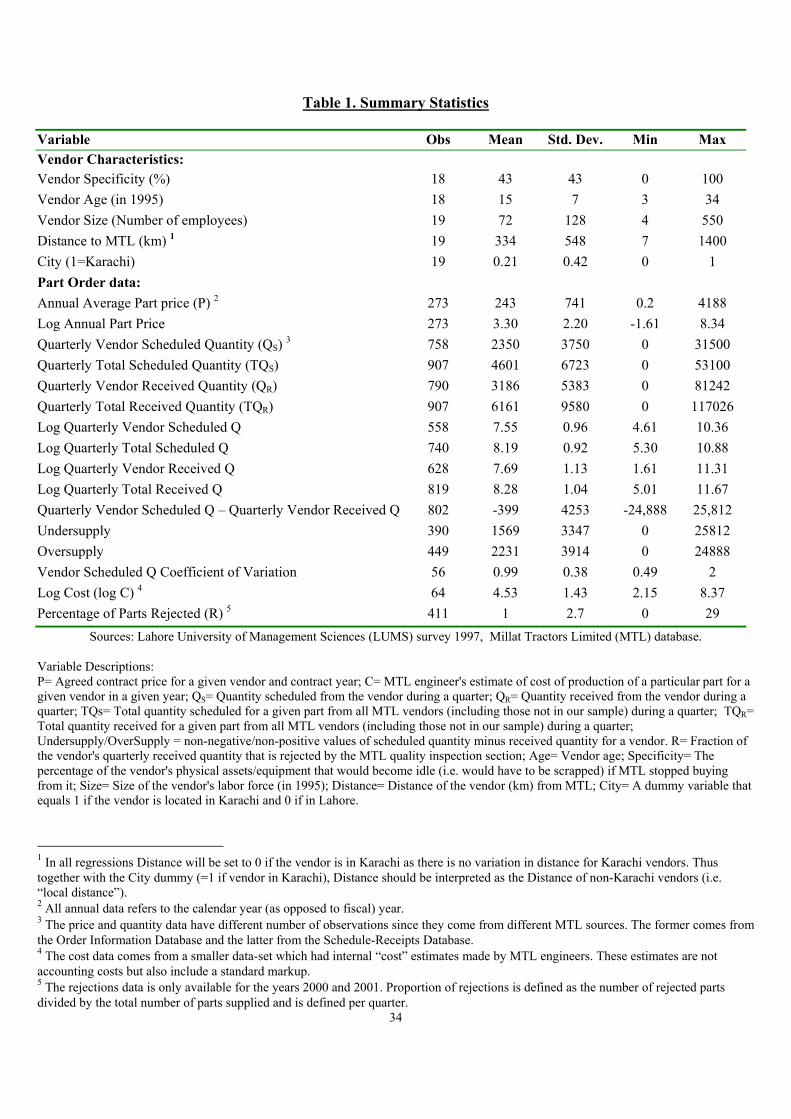
34

Table 1. Summary Statistics

Variable Obs Mean Std. Dev. Min Max Vendor Characteristics: Vendor Specificity (%) 18 43 43 0 100 Vendor Age (in 1995) 18 15 7 3 34 Vendor Size (Number of employees) 19 72 128 4 550 Distance to MTL (km) 1 19 334 548 7 1400 City (1=Karachi) 19 0.21 0.42 0 1 Part Order data: Annual Average Part price (P) 2 273 243 741 0.2 4188 Log Annual Part Price 273 3.30 2.20 -1.61 8.34 Quarterly Vendor Scheduled Quantity (QS) 3 758 2350 3750 0 31500 Quarterly Total Scheduled Quantity (TQS) 907 4601 6723 0 53100 Quarterly Vendor Received Quantity (QR) 790 3186 5383 0 81242 Quarterly Total Received Quantity (TQR) 907 6161 9580 0 117026 Log Quarterly Vendor Scheduled Q 558 7.55 0.96 4.61 10.36 Log Quarterly Total Scheduled Q 740 8.19 0.92 5.30 10.88 Log Quarterly Vendor Received Q 628 7.69 1.13 1.61 11.31 Log Quarterly Total Received Q 819 8.28 1.04 5.01 11.67 Quarterly Vendor Scheduled Q – Quarterly Vendor Received Q 802 -399 4253 -24,888 25,812 Undersupply 390 1569 3347 0 25812 Oversupply 449 2231 3914 0 24888 Vendor Scheduled Q Coefficient of Variation 56 0.99 0.38 0.49 2 Log Cost (log C) 4 64 4.53 1.43 2.15 8.37 Percentage of Parts Rejected (R) 5 411 1 2.7 0 29

Sources: Lahore University of Management Sciences (LUMS) survey 1997, Millat Tractors Limited (MTL) database. Variable Descriptions: P= Agreed contract price for a given vendor and contract year; C= MTL engineer's estimate of cost of production of a particular part for a given vendor in a given year; QS= Quantity scheduled from the vendor during a quarter; QR= Quantity received from the vendor during a quarter; TQs= Total quantity scheduled for a given part from all MTL vendors (including those not in our sample) during a quarter; TQR= Total quantity received for a given part from all MTL vendors (including those not in our sample) during a quarter; Undersupply/OverSupply = non-negative/non-positive values of scheduled quantity minus received quantity for a vendor. R= Fraction of the vendor's quarterly received quantity that is rejected by the MTL quality inspection section; Age= Vendor age; Specificity= The percentage of the vendor's physical assets/equipment that would become idle (i.e. would have to be scrapped) if MTL stopped buying from it; Size= Size of the vendor's labor force (in 1995); Distance= Distance of the vendor (km) from MTL; City= A dummy variable that equals 1 if the vendor is located in Karachi and 0 if in Lahore.

1 In all regressions Distance will be set to 0 if the vendor is in Karachi as there is no variation in distance for Karachi vendors. Thus together with the City dummy (=1 if vendor in Karachi), Distance should be interpreted as the Distance of non-Karachi vendors (i.e. “local distance”). 2 All annual data refers to the calendar year (as opposed to fiscal) year. 3 The price and quantity data have different number of observations since they come from different MTL sources. The former comes from the Order Information Database and the latter from the Schedule-Receipts Database. 4 The cost data comes from a smaller data-set which had internal “cost” estimates made by MTL engineers. These estimates are not accounting costs but also include a standard markup. 5 The rejections data is only available for the years 2000 and 2001. Proportion of rejections is defined as the number of rejected parts divided by the total number of parts supplied and is defined per quarter.

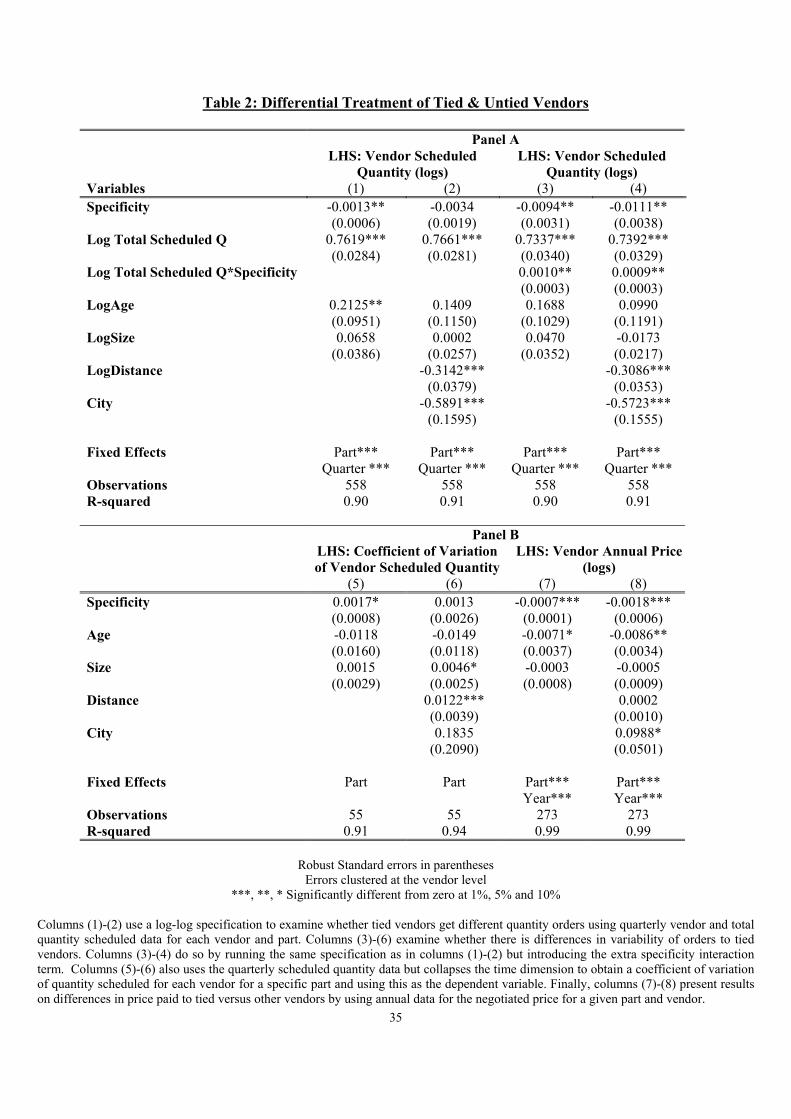
35

Table 2: Differential Treatment of Tied & Untied Vendors

Panel A LHS: Vendor Scheduled

Quantity (logs) LHS: Vendor Scheduled

Quantity (logs) Variables (1) (2) (3) (4) Specificity -0.0013** -0.0034 -0.0094** -0.0111** (0.0006) (0.0019) (0.0031) (0.0038) Log Total Scheduled Q 0.7619*** 0.7661*** 0.7337*** 0.7392*** (0.0284) (0.0281) (0.0340) (0.0329) Log Total Scheduled Q*Specificity 0.0010** 0.0009** (0.0003) (0.0003) LogAge 0.2125** 0.1409 0.1688 0.0990 (0.0951) (0.1150) (0.1029) (0.1191) LogSize 0.0658 0.0002 0.0470 -0.0173 (0.0386) (0.0257) (0.0352) (0.0217) LogDistance -0.3142*** -0.3086*** (0.0379) (0.0353) City -0.5891*** -0.5723*** (0.1595) (0.1555) Fixed Effects Part***

Quarter *** Part***

Quarter *** Part***

Quarter *** Part***

Quarter *** Observations 558 558 558 558 R-squared 0.90 0.91 0.90 0.91 Panel B LHS: Coefficient of Variation

of Vendor Scheduled Quantity LHS: Vendor Annual Price

(logs) (5) (6) (7) (8) Specificity 0.0017* 0.0013 -0.0007*** -0.0018*** (0.0008) (0.0026) (0.0001) (0.0006) Age -0.0118 -0.0149 -0.0071* -0.0086** (0.0160) (0.0118) (0.0037) (0.0034) Size 0.0015 0.0046* -0.0003 -0.0005 (0.0029) (0.0025) (0.0008) (0.0009) Distance 0.0122*** 0.0002 (0.0039) (0.0010) City 0.1835 0.0988* (0.2090) (0.0501) Fixed Effects Part Part Part***

Year*** Part*** Year***

Observations 55 55 273 273 R-squared 0.91 0.94 0.99 0.99

Robust Standard errors in parentheses

Errors clustered at the vendor level ***, **, * Significantly different from zero at 1%, 5% and 10%

Columns (1)-(2) use a log-log specification to examine whether tied vendors get different quantity orders using quarterly vendor and total quantity scheduled data for each vendor and part. Columns (3)-(6) examine whether there is differences in variability of orders to tied vendors. Columns (3)-(4) do so by running the same specification as in columns (1)-(2) but introducing the extra specificity interaction term. Columns (5)-(6) also uses the quarterly scheduled quantity data but collapses the time dimension to obtain a coefficient of variation of quantity scheduled for each vendor for a specific part and using this as the dependent variable. Finally, columns (7)-(8) present results on differences in price paid to tied versus other vendors by using annual data for the negotiated price for a given part and vendor.

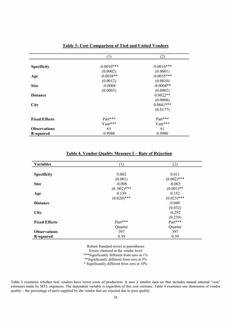
36

Table 3: Cost Comparison of Tied and Untied Vendors

(1) (2) Specificity -0.0010*** -0.0016*** (0.0002) (0.0001) Age -0.0038** -0.0035*** (0.0012) (0.0010) Size -0.0004

(0.0003) -0.0004** (0.0002)

Distance 0.0022** (0.0008)

City

0.0841*** (0.0177)

Fixed Effects Part***

Year*** Part*** Year***

Observations 61 61 R-squared 0.9980 0.9980

Table 4. Vendor Quality Measure I – Rate of Rejection

Variables (1) (2) Specificity 0.002 0.011 (0.001) (0.002)*** Size -0.008 -0.003 (0. 002)*** (0.001)** Age 0.139 0.152 (0.020)*** (0.023)*** Distance 0.049 (0.032) City -0.292 (0.239) Fixed Effects

Part*** Quarter

Part*** Quarter

Observations 397 397 R-squared 0.39 0.39

Robust Standard errors in parentheses

Errors clustered at the vendor level ***Significantly different from zero at 1% **Significantly different from zero at 5% * Significantly different from zero at 10%

Table 3 examines whether tied vendors have lower costs of production. It uses a smaller data-set that includes annual internal “cost” estimates made by MTL engineers. The dependent variable is logarithm of this cost estimate. Table 4 examines one dimension of vendor quality – the percentage of parts supplied by the vendor that are rejected due to poor quality.

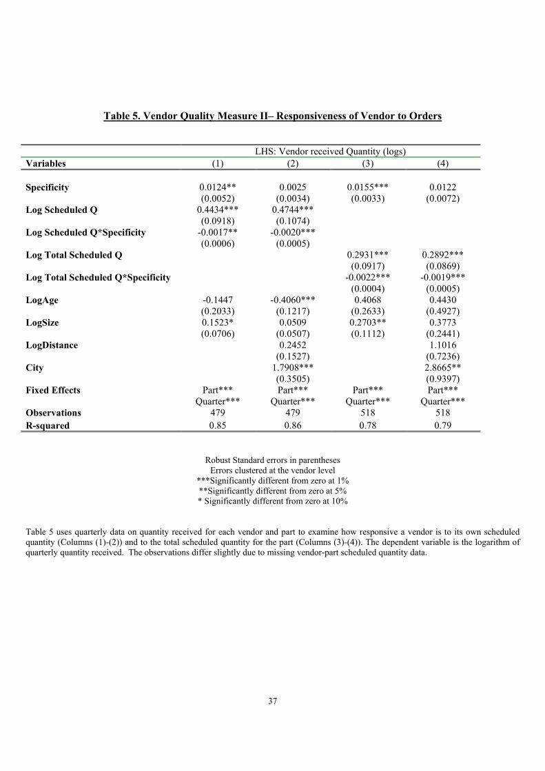
37

Table 5. Vendor Quality Measure II– Responsiveness of Vendor to Orders

LHS: Vendor received Quantity (logs) Variables (1) (2) (3) (4) Specificity 0.0124** 0.0025 0.0155*** 0.0122 (0.0052) (0.0034) (0.0033) (0.0072) Log Scheduled Q 0.4434*** 0.4744*** (0.0918) (0.1074) Log Scheduled Q*Specificity -0.0017** -0.0020*** (0.0006) (0.0005) Log Total Scheduled Q 0.2931*** 0.2892*** (0.0917) (0.0869) Log Total Scheduled Q*Specificity -0.0022*** -0.0019*** (0.0004) (0.0005) LogAge -0.1447 -0.4060*** 0.4068 0.4430 (0.2033) (0.1217) (0.2633) (0.4927) LogSize 0.1523* 0.0509 0.2703** 0.3773 (0.0706) (0.0507) (0.1112) (0.2441) LogDistance 0.2452 1.1016 (0.1527) (0.7236) City 1.7908*** 2.8665** (0.3505) (0.9397) Fixed Effects

Part*** Quarter***

Part*** Quarter***

Part*** Quarter***

Part*** Quarter***

Observations 479 479 518 518 R-squared 0.85 0.86 0.78 0.79

Robust Standard errors in parentheses Errors clustered at the vendor level

***Significantly different from zero at 1% **Significantly different from zero at 5% * Significantly different from zero at 10%

Table 5 uses quarterly data on quantity received for each vendor and part to examine how responsive a vendor is to its own scheduled quantity (Columns (1)-(2)) and to the total scheduled quantity for the part (Columns (3)-(4)). The dependent variable is the logarithm of quarterly quantity received. The observations differ slightly due to missing vendor-part scheduled quantity data.

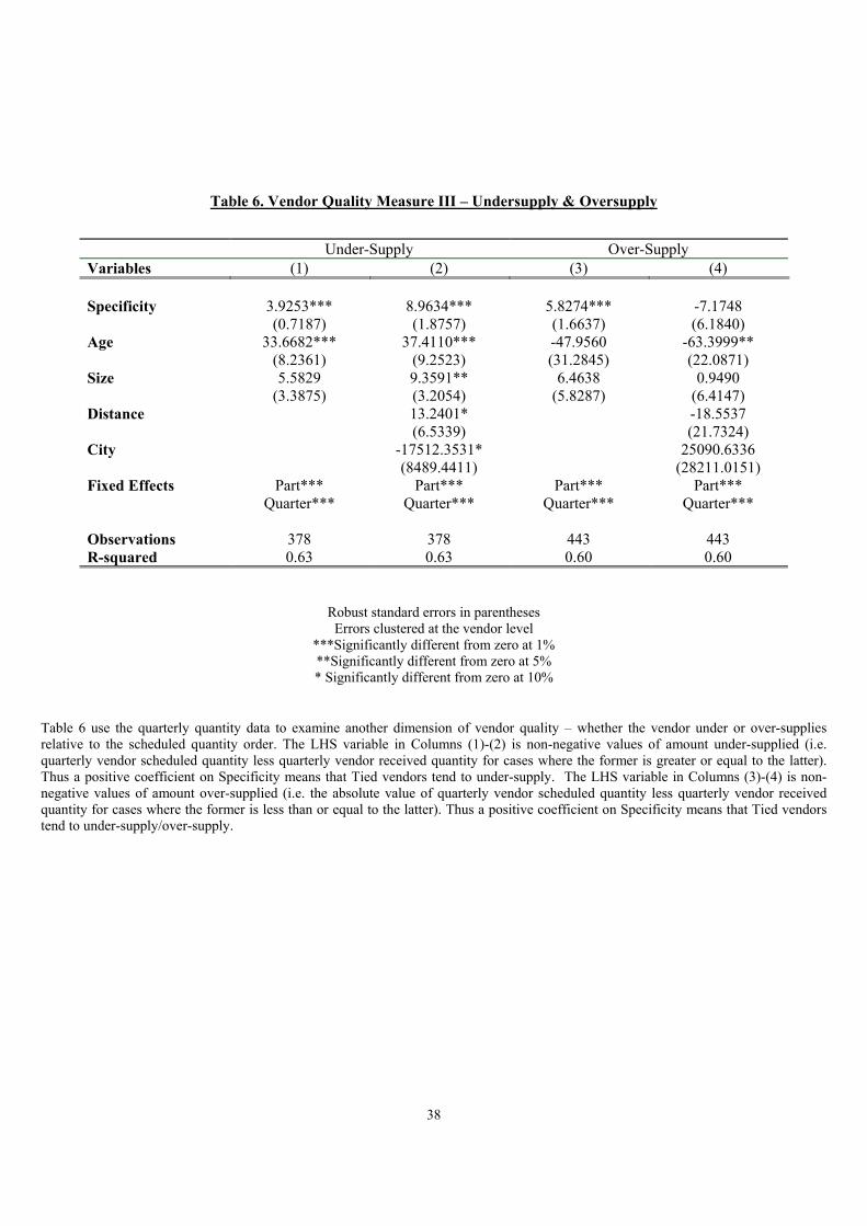
38

Table 6. Vendor Quality Measure III – Undersupply & Oversupply

Robust standard errors in parentheses Errors clustered at the vendor level

***Significantly different from zero at 1% **Significantly different from zero at 5% * Significantly different from zero at 10%

Table 6 use the quarterly quantity data to examine another dimension of vendor quality – whether the vendor under or over-supplies relative to the scheduled quantity order. The LHS variable in Columns (1)-(2) is non-negative values of amount under-supplied (i.e. quarterly vendor scheduled quantity less quarterly vendor received quantity for cases where the former is greater or equal to the latter). Thus a positive coefficient on Specificity means that Tied vendors tend to under-supply. The LHS variable in Columns (3)-(4) is non-negative values of amount over-supplied (i.e. the absolute value of quarterly vendor scheduled quantity less quarterly vendor received quantity for cases where the former is less than or equal to the latter). Thus a positive coefficient on Specificity means that Tied vendors tend to under-supply/over-supply.

Under-Supply Over-Supply Variables (1) (2) (3) (4) Specificity 3.9253*** 8.9634*** 5.8274*** -7.1748 (0.7187) (1.8757) (1.6637) (6.1840) Age 33.6682*** 37.4110*** -47.9560 -63.3999** (8.2361) (9.2523) (31.2845) (22.0871) Size 5.5829 9.3591** 6.4638 0.9490 (3.3875) (3.2054) (5.8287) (6.4147) Distance 13.2401* -18.5537 (6.5339) (21.7324) City -17512.3531* 25090.6336 (8489.4411) (28211.0151) Fixed Effects Part***

Quarter*** Part***

Quarter*** Part***

Quarter*** Part***

Quarter*** Observations 378 378 443 443 R-squared 0.63 0.63 0.60 0.60

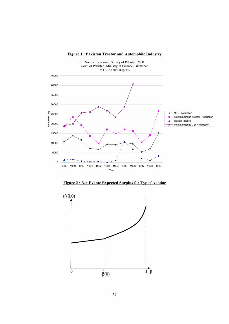
39

0

5000

10000

15000

20000

25000

30000

35000

40000

45000

1988 1989 1990 1991 1992 1993 1994 1995 1996 1997 1998 1999Year

Prod

uctio

n (n

o) MTL ProductionTotal Domestic Tractor Production Tractor ImportsTotal Domestic Car Production

s∗(β,θ)

β(θ)^ β0 1

Figure 1 : Pakistan Tractor and Automobile Industry

Source: Economic Survey of Pakistan,2000 Govt. of Pakistan, Ministry of Finance, Islamabad.

MTL. Annual Reports

Figure 2 : Net Exante Expected Surplus for Type θ vendor