subgrid combustion modeling for premixed turbulent ... · subgrid combustion modeling differs from...

Copyright© 1997, American Institute of Aeronautics and Astronautics, Inc.

Subgrid Combustion Modeling for Premixed Turbulent ReactingFlows *

Thomas M. Smith '''and Suresh Menon *School of Aerospace EngineeringGeorgia Institute of Technology

Atlanta, Georgia 30332-0150email: [email protected]

AbstractTwo combustion models for turbulent premixed com-bustion in the flamelet regime are developed for un-steady simulations. The first model is a convensional Gequation flamelet model and the main issues discussedare the subgrid closure. The second model is basedon the Linear-Eddy Model. Both models are used insimulation of turbulent stagnation point flames. Theheat release and turbulence intensity are varied. Timeaveraged statistics from convensional simulations showgood qualitative agreement with experiments and thenormalized turbulent flame speed agrees well with theexperimental data. Counter-gradient scalar diffusion isobserved in high heat release, low turbulence intensityflames. This raises the question about how importantthe gradient diffusion approximation is to these results.Preliminary results from LES-LEM simulations involv-ing moderate heat release and high turbulence inten-sities are reported. The key role of the front trackingalgorithm is demonstrated. Qualitative trends in theburning rates with varying turbulence intensity is alsodemonstrated.

1 IntroductionOf central importance to the understanding and pre-diction of turbulent flame propagation physics areflame/turbulence responses to varying laminar flamespeeds (SL), turbulence intensities (u1), and turbulencelength scales (/). While SL may be assumed constantin many flows (flamelet approximation), turbulence ve-locity and length scales vary greatly and so flamelet re-sponse to a changing hydrodynamic field is a local phe-

"Copyright ©1998 by T. M. Smith and S. Menon. Publishedby the American Institute of Aeronautics and Astronautics, Inc.,with permission.

tGraduate Research Assistant, Student Member, AIAA* Professor, Senior Member, AIAA

nomena. In addition, alteration of the hydrodynamicfield, mainly due to dilatation and increased viscous ef-fects occur simultaneously. For these reasons, steadystate approaches for predicting flame/turbulence inter-actions are limited. The problem may be solved, intheory, by direct numerical simulation (DNS). However,DNS is highly restricted to a narrow band of length andtime scales due to available computational resource lim-itations.

Large-Eddy simulation (LES) is an emerging tech-nology that bridges the gap between (DNS) and theReynolds Averaged Navier-Stokes (RANS) approach.The concept of LES is based on physical argumentsabout resolved and unresolved (subgrid) scales existingin the flow. These physical arguments are summarizedby Ferziger (1983): 1) The largest eddies interact withthe mean flow while the small eddies are created bynonlinear interactions among the large eddies. 2) Thestructure of large scales is strongly dependent on ge-ometry and are therefore anisotropic (usually vortical)while the small scales are more isotropic and univer-sal. 3) Large eddy time scales approximate the timescales of the mean flow while subgrid time scales aremuch shorter since small eddies are created and de-stroyed more rapidly than large scales. 4) Most of thetransport of mass, momentum, energy, and concentra-tions is due to the large scales while small scales mainlydissipate fluctuations in these quantities.

The consequences of these arguments are: 1) Largescales are much harder to model and it is unlikely thata universal model may be found. On the other hand,small scales are much easier to model due to their uni-versal character and a model for small scales is morelikely to be found. 2) Most of the transport is computeddirectly. 3) The computational cost increases comparedto RANS. This leads to the concept of large-eddy sim-ulation where the large scales are directly computedand the effect of the small scales on the large scales ismodeled.


Subgrid combustion modeling differs from subgridturbulence modeling in that usual assumptions madefor momentum and energy equation closures are sus-pect for reacting scalars. Namely, the gradient diffusionassumption (Boissenesq approximation, where an ap-parent viscosity called the eddy viscosity and the meanstress tensor are combined to model the Reynolds stresstensor) may be valid for momentum and energy so thatrelatively simple models may be used. However, in thecase of diffusive-reactive scalars, combustion is domi-nated by mixing processes and premixed flamelet prop-agation rates are greatly influenced by micro-scale wrin-kling. Micro-scale mixing and flame surface wrinklingare not adequately modeled by gradient diffusion. Inaddition, counter-gradient diffusion has been observedin reacting flows having significant heat release.

In an earlier paper (Smith and Menon, 1997) thecomputational methodology for simulating stagnationpoint flames was demonstrated. In that study, theflame propagation was described using an uncoupledLES-LEM approach. This paper continues the devel-opment of the stagnation point flame simulations us-ing both the conventional flamelet model and the LES-LEM method of computing turbulent reacting flows.Some important features of the LES-LEM methodol-ogy include; appropriate characterization of unresolvedfine-scale wrinkling and flamelet burning, the resolvedscale transport of the progress variable by the resolvedscale turbulence and thermodynamic coupling betweenthe subgrid and the resolved field.

Stagnation point flames have several advantages thatare exploited in order to evaluate this modeling ap-proach. First, the flow is stationary and, thus, the flameposition and propagation rate are steady. The steadynature of these flows allows for statistical propertiesto be analyzed. Since the subgrid model is stochastic,precise evolution of the burning surface is not available.Instead a stationary turbulent flame structure is com-puted that is suitable for comparison with existing ex-perimental data. Secondly, the turbulence intensity andheat release can be parameterized to test how the sub-grid combustion model and the resolved scale progressvariable respond to these hydrodynamic inputs.

2 Model Formulation

The LES-LEM modeling approach is described in thissection. The model consists of the conventional LESframework, the subgrid combustion model and the thecoupling mechanism that links subgrid combustion tothe LES resolved field solution and resolved field con-vection to the transport of LEM cells.

2.1 Large-Eddy SimulationThe equations of LES are the mass weighted spatiallyfiltered mass, momentum, energy, and species equa-tions. Subgrid terms are a result of filtering nonlin-ear terms in the equations and models must be foundfor them. Of particular interest is the filtered speciesequation which contains a subgrid flux that is due tothe unresolved turbulent velocity field and the mean re-action rate. Both of thesejmknown terms are trouble-some. The subgrid flux pfujYJt— UiYk] is the transport ofspecies mass fraction by subgrid scale turbulence and isresponsible for micro-scale mixing. The mean reactionrate (J/, depends on correlations between resolved andunresolved temperature (T, T"), and between resolvedand unresolved species (Yf,, Y^) correlations and is verydifficult to evaluate. A common practice is to evaluatethe probability density function (pdf) of the reactionrate as a function of resolved variables. Though a closedform expression for u/t can be found, these methods aremainly used for steady state calculations and modelingmicro-scale mixing is not straight forward.

The current approaches replace the filtered speciesequations with a conventional flamelet model referredto as the G equation and a subgrid combustion modelwhere the scalars evolve according to diffusion-reactionequations and stochastic rearrangement events repre-senting turbulent stirring.

2.2 G-Equation Flamelet ModelThe flamelet assumption describes a regime in premixedcombustion that is often encountered in practical com-bustion devices. Within the flamelet assumption, theflame thickness (Si) is small compared to the smallestdynamic scale (77, the Kolmogorov scale) of turbulenceand the characteristic burning time (rc) is small com-pared to the characteristic flow time (T). As a result,the flame structure remains unaltered and the flamecan be considered a thin front propagating at a speeddictated by the mixture properties that is wrinkled andconvected by the flow. A model equation that describesthe propagation of a thin flame by convective transportand normal burning (self propagation by Huygens' prin-ciple) has been introduced called the G-field equation(Williams, 1985; Kerstein et ai, 1988)

dt (1)

where G is a progress variable that defines the loca-tion of the flame, u is the mass averaged velocity vec-tor and SL is the local laminar flame speed. Equation(1) describes the convection of a level surface, definedas G = G0, by the fluid velocity while simultaneouslyundergoing propagation normal to itself at a speed SL


according to Huygens' principle. In the flow field, thevalue of G is in the range [0,1] and in flame front model-ing, G exhibits a step function like behavior, separatingthe burnt region (G < G0) from the unburned region(G > GO). G is assigned the value of unity in the un-burned region and zero in the burnt region with thethin flame identified by a fixed value of 0 < G0 < 1.In the finite-volume numerical approach, an equivalentequation is written

dpGdt (2)

where p0 is the reference reactant density and S°L isthe undisturbed laminar flame speed. The relation-ship, p0S°L = pSi is an expression of mass conservationthrough the flame.

Upon filtering

dpGdt

+ V • puG = p0Si\VG\ - V • (p[uG - uG]). (3)

The unresolved transport term is modeled using a gra-dient assumption (Im, 1995; Im et al., 1997 and Pianaet al., 1997)

(4)

where pt is an eddy viscosity and ScG is a Schmidtnumber. At first glance, the gradient closure approx-imation appears to clearly violate the physics of tur-bulent transport given that counter-gradient diffusiondominates the transport of scalar fluxes in many situa-tions. However, it must be kept in mind that counter-gradient transport is a large scale phenomena (Bray,1995) and in the LES methodology, the large scales aredirectly computed and therefore, counter-gradient dif-fusion should be accounted for despite the subgrid clo-sure assumed. This, of course, will require evaluation.In addition, counter-gradient diffusion is produced bythe preferential acceleration of lighter parcels of fluid asopposed to heavier parcels by the mean pressure gra-dient. Given the current subgrid modeling technology,pressure gradient effects are not included in the closuremodels and therefore the ability to produce counter-gradient diffusion is absent from all models that neglectpressure effects.

For closure of the source term, Yakhot's RNG modelis used (Yakhot, 1988; Menon and Jou, 1991). Thismodel is an analytical expression for the turbulent flamespeed as a function of turbulence intensity (ut/SL =exp[u'2/Uf]) obtained from Eq. (1). For flamelet com-bustion, ^ = jj*- where At and AI are the turbu-lent and laminar flame areas respectively, and thereforeYakhot's model is an estimate of the flame wrinklingdue to the turbulence intensity. Therefore, in the LES

context, the propagation rate is no longer p0S°L but isinstead replaced by p0Uj where uj is obtained from(uj/SL = exp[(u'sgs)2/(uf)2}) which is the subgrid tur-bulent burning rate that accounts for unresolved flamewrinkling. The turbulence intensity appearing in theturbulent flame speed model is the subgrid turbulenceintensity, usgs = v/f &S£rs where ksgs is the subgrid tur-bulent kinetic energy given by, ksgs — ^[uiui — uiui].Note that usgs ^ u'{ which represents the fluctuatingpart of Ui. A model equation for the subgrid turbu-lent kinetic energy is discussed in Smith and Menon(1997). It was argued there that in two-dimensionalconstant flame speed simulations, the subgrid kineticenergy is negligible and therefore, subgrid closure termscan be neglected. In the present study, the subgridterms are included and the subgrid turbulence intensityis retained to provide a measure of the subgrid flamespeed through Yakhot's model.

This model assumes that the flame is a thin sheethaving no internal structure and, therefore, is applica-ble only in the flamelet combustion regime. Further-more, it does not take into account flame stretchingeffects and so cannot predict extinction. However, ithas been shown that the model compares well with ex-perimental data in the low to moderately high u'/SLrange and also predicts (in reasonable agreement withdata) a rapid increase in Ut/SL at low u'/Si and then abending slope at high u'/SL (Yakhot, 1988). The sourceterm for the filtered G equation becomes

Pout\VG\. (5)

Thermodynamic coupling is through the internal en-ergy e = cvf+ Aft/G, where Aft/ = cp(Tp - Tf) isthe heat of formation, cv and cp are the specific heatsat constant volume and pressure respectively. In casesof non-zero heat release, the internal energy is now afunction of G, e = cvf + ft/G where ft/ = cp(Tp - T/)is a heat release parameter. In this case ft/ should bea heavy side function of G, however, this produces anumerical instability when the flame front is steeplyvarying. Menon (1991) has pointed out that the lineardependence on G results in a distributed heat releasethat tracks the flame and does not cause significant er-ror as long as the front is not a broad front.

2.3 Linear-Eddy ModelThe linear-eddy model of Kerstien (1991) was originallydeveloped as a mixing model for diffusive scalars. Itwas later shown capable of predicting turbulent com-bustion processes in flows having a large degree of sym-metry. In recent years it has been adapted to LESas a subgrid combustion model for turbulent diffusion


flames (Calhoon and Menon 1996; 1997). It has alsobeen shown capable of characterizing premixed turbu-lent flame propagation in isotropic flows (Smith andMenon; 1996a, 1996b). In this paper, the LEM isadopted as a subgrid model for premixed flame propa-gation in the laminar flamelet regime.

The LEM model can be described as a direct sim-ulation of diffusive-reactive scalars in isotropic tur-bulence on a linear domain. A system of reaction-diffusion equations that describe the continuous evo-lution of scalars (not containing an explicit velocity)on a line are subjected to instantaneous rearrangementevents each one mimicking the action of a single eddy.For flamelet regime combustion (Si « rj), using theG — field equation, a model for flamelet combustion us-ing the linear-eddy approach is formulated (designatedGLEM). GLEM models laminar burning by the propa-gation equation (Menon and Kerstein, 1992; Smith andMenon, 1996b)

^ = 5L|VG|. (6)

This equation tracks the propagation of a single valueof G between G/ue; < G0 < Gprod, where Gjuei =1 and Gprod = 0. G0 is a pre specified level surfacerepresenting the location of the flame. Therefore, flamepropagation is described by one scalar instead of N + I(Menon and Kerstein, 1992). The flame speed SL is alsoa pre specified constant which accounts for all of thephysio-chemical properties of the mixture. Since LEMresolves even step-like fronts, no dissipation mechanismis necessary to prevent false minima from occurring.

Stochastic rearrangements of scalar fields is accom-plished by the triplet map, Kerstein (1991). The re-arrangement events are governed by three parameters;location of mapping event, size of the event and the fre-quency per unit length of events. The parameters areobtained by equating the total diffusivity of a randomwalk of a marker particle with the turbulent diffusivity(u'l) in inertial range turbulence. This stirring processwrinkles the subgrid G field increasing the per LES cellburning rate, which is estimated as the number of flamecrossings (G0) in the LES cell. For a more detailed de-scription see Smith and Menon (1997).

2.4 Linear-Eddy SubgridModel

Combustion

The remaining component in the LES-LEM formula-tion is the coupling between the subgrid combustionand the resolved scale flow quantities. LES-LEM cou-pling is accomplished by resolved scale convection andby specifying the subgrid Re and length scale.

Large scale convection between two adjacent LEScells is handled by splicing subgrid cells from a donat-

ing LES cell to a receiving LES cell (Menon et al., 1994;Calhoon and Menon, 1996). The splicing algorithm(i) calculates the volume flux to be transferred acrossthe LES cell interface (in a finite volume formulation)based on the resolved velocity and subgrid turbulenceintensity («,• -f u'ags ) , (ii) removes an equivalent numberof LEM cells from the donor LES cell, and, (iii) addsthem to the receiving LES cell. The rate of transfer isbased on the convective time scale of the resolved ve-locity, Atccw = min{AxLEs/(ui + u'igi)}, (Calhoonand Menon, 1996). Spurious scalar diffusion can oc-cur when a group of LEM cells are spliced from one celland placed adjacent to cells in another LES cell. This isbecause the scalar may not be continuous at the inter-face. Calhoon advocated the use of subgrid partitionsto help eliminate this problem. In the present study,a new approach is taken. Since spliced cells take thevalue of 0 or 1, upon insertion into the receiving LEScell, the new cells can be placed adjacent to cells havingthe same value as the cell on the end of the segment.Thus, no artificial flamelet is created by splicing. Thiseliminates spurious diffusion altogether. In addition,convecting scalar values of either 0 or 1 was found togreatly reduce spurious diffusion when the mean flow isnot aligned with a grid direction. This issue becomesless important as Resgs increases. Resgs is obtained di-rectly from uags — \l |fcs0s (not to be confused with u'or u").

Two different methods of thermodynamic couplingare currently under investigation for LES-LEM. Thefirst method is described in Calhoon and Menon (1996).In this method LEM-LES thermodynamic coupling re-lates the progress of the flame in each LES cell to theresolved internal energy, e = cvT + AhfG, where Gis the Favre filtered G that is obtained from the sub-grid scalar field, A/i/ = cp(Tproci — T/ue/) is the heat offormation, cv and cp are the specific heats at constantvolume and pressure respectively. The second methodreplaces the heat of formation contained in the totalenergy with a source term. The source term can becalculated exactly from the unfiltered subgrid field as

(7)is

AhfPoSL\VG\ =

where ISGS is the subgrid resolution and Axthe subgrid cell spacing.

3 Simulation of Stagnation PointFlames

The numerical simulations of stagnation point flameswere designed to mimic the experiments of Cho et al.


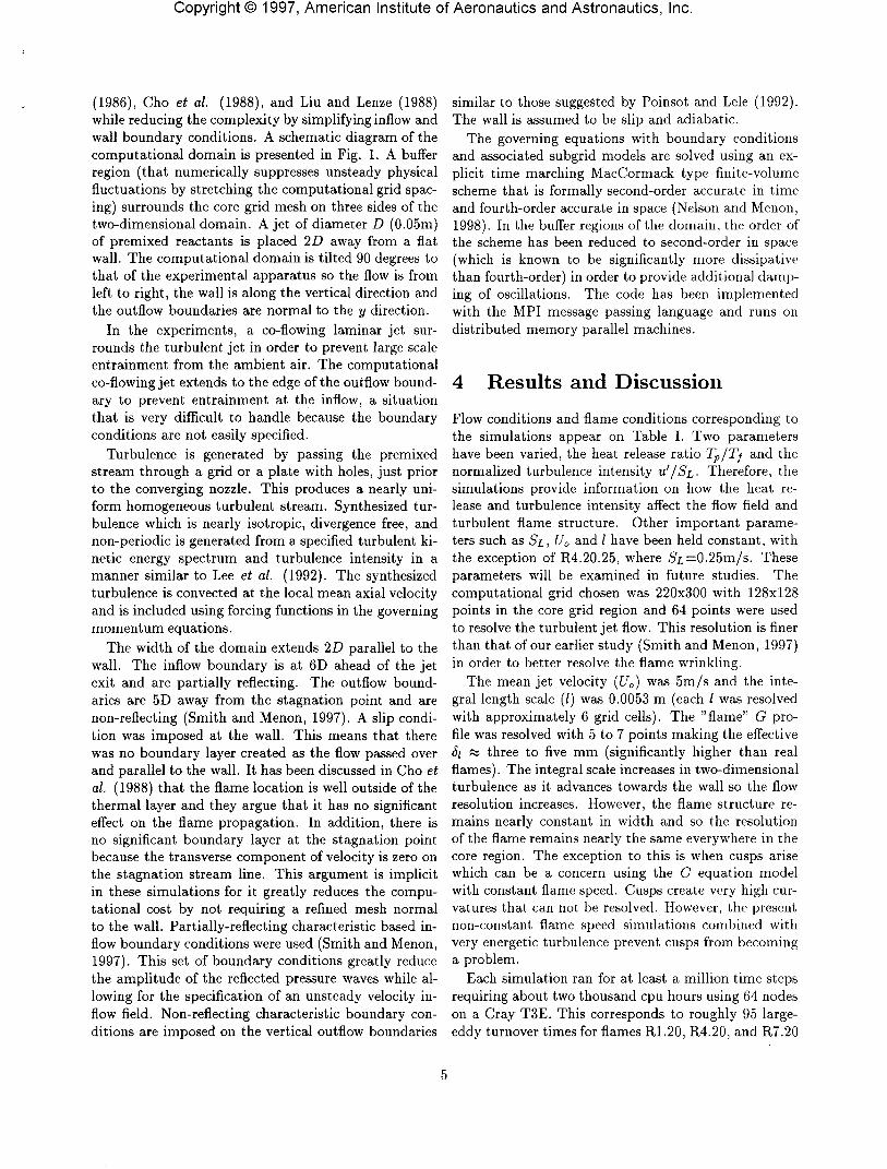
(1986), Cho et al. (1988), and Liu and Lenze (1988)while reducing the complexity by simplifying inflow andwall boundary conditions. A schematic diagram of thecomputational domain is presented in Fig. 1. A bufferregion (that numerically suppresses unsteady physicalfluctuations by stretching the computational grid spac-ing) surrounds the core grid mesh on three sides of thetwo-dimensional domain. A jet of diameter D (0.05m)of premixed reactants is placed ID away from a flatwall. The computational domain is tilted 90 degrees tothat of the experimental apparatus so the flow is fromleft to right, the wall is along the vertical direction andthe outflow boundaries are normal to the y direction.

In the experiments, a co-flowing laminar jet sur-rounds the turbulent jet in order to prevent large scaleentrainment from the ambient air. The computationalco-flowing jet extends to the edge of the outflow bound-ary to prevent entrainment at the inflow, a situationthat is very difficult to handle because the boundaryconditions are not easily specified.

Turbulence is generated by passing the premixedstream through a grid or a plate with holes, just priorto the converging nozzle. This produces a nearly uni-form homogeneous turbulent stream. Synthesized tur-bulence which is nearly isotropic, divergence free, andnon-periodic is generated from a specified turbulent ki-netic energy spectrum and turbulence intensity in amanner similar to Lee et al. (1992). The synthesizedturbulence is convected at the local mean axial velocityand is included using forcing functions in the governingmomentum equations.

The width of the domain extends 21? parallel to thewall. The inflow boundary is at 6D ahead of the jetexit and are partially reflecting. The outflow bound-aries are 5D away from the stagnation point and arenon-reflecting (Smith and Menon, 1997). A slip condi-tion was imposed at the wall. This means that therewas no boundary layer created as the flow passed overand parallel to the wall. It has been discussed in Cho etal. (1988) that the flame location is well outside of thethermal layer and they argue that it has no significanteffect on the flame propagation. In addition, there isno significant boundary layer at the stagnation pointbecause the transverse component of velocity is zero onthe stagnation stream line. This argument is implicitin these simulations for it greatly reduces the compu-tational cost by not requiring a refined mesh normalto the wall. Partially-reflecting characteristic based in-flow boundary conditions were used (Smith and Menon,1997). This set of boundary conditions greatly reducethe amplitude of the reflected pressure waves while al-lowing for the specification of an unsteady velocity in-flow field. Non-reflecting characteristic boundary con-ditions are imposed on the vertical outflow boundaries

similar to those suggested by Poinsot and Lele (1992).The wall is assumed to be slip and adiabatic.

The governing equations with boundary conditionsand associated subgrid models are solved using an ex-plicit time marching MacCormack type finite-volumescheme that is formally second-order accurate in timeand fourth-order accurate in space (Nelson and Menon,1998). In the buffer regions of the domain, the order ofthe scheme has been reduced to second-order in space(which is known to be significantly more dissipativethan fourth-order) in order to provide additional damp-ing of oscillations. The code has been implementedwith the MPI message passing language and runs ondistributed memory parallel machines.

4 Results and DiscussionFlow conditions and flame conditions corresponding tothe simulations appear on Table I. Two parametershave been varied, the heat release ratio Tp/Tj and thenormalized turbulence intensity U'/SL- Therefore, thesimulations provide information on how the heat re-lease and turbulence intensity affect the flow field andturbulent flame structure. Other important parame-ters such as Si, U0 and / have been held constant, withthe exception of R4.20.25, where 5z,=0.25m/s. Theseparameters will be examined in future studies. Thecomputational grid chosen was 220x300 with 128x128points in the core grid region and 64 points were usedto resolve the turbulent jet flow. This resolution is finerthan that of our earlier study (Smith and Menon, 1997)in order to better resolve the flame wrinkling.

The mean jet velocity (£/„) was 5m/s and the inte-gral length scale (/) was 0.0053 m (each / was resolvedwith approximately 6 grid cells). The "flame" G pro-file was resolved with 5 to 7 points making the effectiveSi « three to five mm (significantly higher than realflames). The integral scale increases in two-dimensionalturbulence as it advances towards the wall so the flowresolution increases. However, the flame structure re-mains nearly constant in width and so the resolutionof the flame remains nearly the same everywhere in thecore region. The exception to this is when cusps arisewhich can be a concern using the G equation modelwith constant flame speed. Cusps create very high cur-vatures that can not be resolved. However, the presentnon-constant flame speed simulations combined withvery energetic turbulence prevent cusps from becominga problem.

Each simulation ran for at least a million time stepsrequiring about two thousand cpu hours using 64 nodeson a Cray T3E. This corresponds to roughly 95 large-eddy turnover times for flames R1.20, R4.20, and R7.20


and roughly 6.3 flow through times for all flames, wherea flow through time is defined as 4D/U0. Statistics weregenerated from the final 80% of the data.

Figures 2a and 2b are snapshots of two flow simu-lations R7.5 and R7.20 highlighting the difference inthese wrinkled flames with varying u'/Si- Flame R7.5is nearly plannar and shows only small perturbations tothe surface while flame R7.20 is highly convoluted, po-sitioned further upstream away from the wall. It is alsoclear from the vorticity contours that more turbulencesurvives into the post flame region in flame R720. Fig-ure 3 is taken from a video tape provided by Dr. R. K.Cheng. In these tomographic images the flow is frombottom to top, the light colored portion is reactants,the black, products. The flame structures are similarhowever it is clear that the experimental flames exhibithigher curvatures than do these simulations.

The Reynolds time averaged mean axial velocities fordifferent simulations are shown in Figs. 4a-4c. In Fig.4a, the turbulence intensity has been varied for a con-stant heat release of Tp/Tj = 4. Note that the veloc-ity decreases non-linearly at the jet exit and reachesa linear decay only near the wall. This is due to thezero divergence at the jet nozzle. For low u'/Si, theacceleration in velocity through the flame is distinct.As u''/Si increases and the flame normal direction be-comes more random this organized acceleration is re-duced. The amount of heat release is varied for constantU'/SL in Figs. 4b and 4c. The effect of increasing heatrelease is an increased acceleration through the flameand a mean flame positioned further from the wall. Athigher intensity (Fig. 4c), the acceleration is again re-duced compared to the lower intensity case. However,the flame position is even further away from the walldue to the increased burning rate.

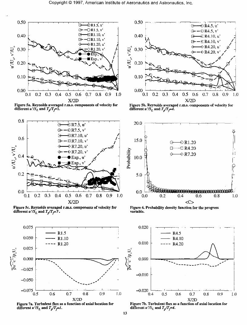
The Reynolds time averaged r.m.s. axial velocitycomponents are shown as a function of turbulence in-tensity holding the heat release constant in Figs. 5a-5c.Only a qualitative comparison with Cho et al. (1986)is shown since, the inflow intensity is not matched be-tween the experiments and the simulations. The mostimportant difference between these two-dimensionalsimulations and the axisymmetric experiments is thedecay in turbulence intensity. Nevertheless, near-flameand post-flame characteristics are very similar. In allcases v' increases in the vicinity of the wall. It shouldbe kept in mind that the wall boundary is a velocityslip condition, so v' does not decay to zero at the wallas it does in reality. In the low U'/SL cases, u' increasesthrough the flame.

In summary, the analysis of the time averaged veloc-ity data, suggest that the effect of heat release on theflow is significant at low U'/SL and diminishes as U'/SLincreases. The flame structure is examined next.

In the beginning of this section it was stated thatthe G structure was resolved over five to seven cellsmaking these simulated flames much thicker than theirexperimental counter parts. As the two-dimensionalturbulence evolves the small scales quickly dissipate re-sulting in larger length scales at the flame zone than atthe jet exit. Flamelet combustion is implicitly assumedby our choice of flamelet approach. From Table I, theDamkohler numbers (Da = ( l / S i ) / ( u ' / S L ) ) based onthe flame thickness, Jj = v/SL, where v is the reactantkinematic viscosity, are all greater than unity and theKarlovitz numbers (Ka = (£;/f?)2) where 77 = / /Re3 /4

is the Kolmogorov length scale and Re = u'l/i/, rangefrom 0.18 to 1.42 for the SL =0.5m/s flames. TheseKa numbers are somewhat high but the small scalesare increasing as the flow evolves. To test whetherthe flamelet assumption is valid the probability den-sity function (pdf) of the progress variable defined asC = 1 — G is plotted as a function of the mean progressvariable < C > for the high intensity simulations in Fig.6. In all the cases, the pdf is bimodal which means thatwithin the turbulent flame zone the progress variable isoverwhelming either unreacted or fully reacted. Thisresult confirms that the flamelet assumption is validfor these conditions.

The turbulent flux that appears as an unclosed termin the Favre averaged species equation is an importantterm that accounts for the turbulent diffusion of re-acting scalars and must be modeled. It is common toassume a gradient diffusion model

pu"c" = pu"c" = dc(8)

where fj.t is an eddy viscosity, ac is the turbulentSchmidt number and #,- is a Cartesian coordinate com-ponent. The presence of counter-gradient diffusion inturbulent premixed combustion has been well estab-lished in theory (Libby and Bray, 1981), experiments(Cho et al., 1988; Li et al., 1996) and in direct numeri-cal simulation (DNS) (Veynante et al. 1995, 1997). Theturbulent flux normalized by the reactant density (p0)and the mean jet velocity (U0) are shown in Figs. 7a-7d.The abcissa is normalized by the distance from the jetexit to the wall (2D). In Fig. 7a, the turbulence inten-sity is varied with no heat release. The turbulent fluxis of gradient type (-) for all three cases increasing inmagnitude as the intensity increases. In Fig. 7b pu"c"changes from counter-gradient (+) (low u') to gradient(higher u') (-). Also note that the flame brush becomesbroader with increasing u'. In Figs. 7c and 7d, theheat release is varied for the low u' flames and the highu' flames. The trends are the same. Gradient diffusionoccurs in the no heat release cases and counter-gradientdiffusion is observed for higher heat release. The high

6


u' flames are thicker than the low u' flames and the highheat release flames are pushed away from the wall.

Another way to look at the effect of heat release andU'/SL on the turbulent flux is to plot it in progress vari-able space where all the flames are mapped to the av-erage C. These are shown in Figs. 8a-8d. Of particularinterest is Fig. 8d in which both gradient and counter-gradient diffusion exists in the high heat release, highu' flame (R7.20).

In Figs. 9a-9c, the flame surface densities (£) fordifferent Tp/Tj are plotted at U'/SL = 1,2,4 respec-tively. In two-dimensions, this is the flame length perunit area. It has a unit of I/mm which is customaryin the experimental literature. There are several waysto calculate this quantity (Trouve et al. 1994; Peters1997). The method chosen here is to define a smallrange in the progress variable. C is divided into a num-ber of equal partitions. From the gradient |V(7| at eachlocation in the flame brush, if C is within the desiredrange |V(7| is stored in the appropriate C partition andaveraged. With the exception of some scatter towardsthe back of the flame (C w 0.8) for the no heat releasecases, £ tends to converge. This trend is observed inexperiments of stagnation point flames.

The curvature distribution is compared to the experi-mental data of Shepherd and Ashurst (1992) in Fig. 10,with all of their flames at u' /Si < 1- The pdf of flamecurvature collapses when normalized by the r.m.s. cur-vature. The simulated flames show similar magnitudebut differ significantly from the experimental flames.Flame R7.10 matches more closely in both U'/SL andheat release than do the other two flames and it matcheswith the experimental flames reasonably well in shapebut not magnitude.

The normalized turbulent flame speed ut/Sz,, is plot-ted as a function of U'/SL in Fig. 11. The turbulentflame speed is defined as the value of < U > where theslope begins to change (Cho et al. 1986; Liu and Lenze,1988). For no heat release cases, The value of < U > ischosen where < C > obtains a value of 0.02. This valuewas determined from averaging < C > for the heat re-lease cases once the location had been determined fromwhere the slope changed. These two-dimensional sim-ulations compare well with the data from Cho et al.(1986) but under predict the data of Liu and Lenze,(1988) significantly.

4.1 LES-LEM Flame PropagationTo the best of the authors' knowledge, this work rep-resents the first attempted premixed unsteady reactingsimulations of stagnation point flames. Though mostlyqualitative in nature, the agreement with experimentaldata is quite encouraging. Simulations like these can

provide a database for the evaluation of other modelssuch as the LES-LEM model which has a range of ap-plicability exceeding the flamelet regime.

The LEM is calibrated using a stand alone modelof flame propagation into isotropic turbulence (Smithand Menon 1996). One calibration constant adjusts thestirring frequency to match the burning rates observedin stagnation point flame experiments. This calibra-tion constant is then used in the subgrid model. Thecalibration curves are shown in Fig. 12.

Figures 13a and 13b show the effect of artificial flamereduction on propagation of a laminar flame. The flameis being convected to the right while burning into thefuel on the left. Without the flame reduction algorithm,the flame shape becomes distorted.

Figure 14 shows a snapshot vorticity contours andthe filtered subgrid G field. The resolution is 25% lessthan the conventional G simulations and the U'/SL — 8,Re=2QQ and Tp/T} = 4. The flame structure looks sim-ilar to Fig. 2b though scales of wrinkling are notice-ably smaller resulting in less resolved flame area. Thesmaller flame area is compensated for by the subgridwrinkling.

To study the propagation mechanisms in the LES-LEM approach, three propagation speeds are defined.Collection of data only includes the core region whichis defined as the twice the width of the forced jet. Thefirst is ALES/AL, the resolved scale area ratio. Forthis geometry, AL is simply the width of the domain(which is the twice the width of the forced jet). Inflamelet combustion, the area ratio is approximatelythe ratio of the turbulent to laminar flame speed. Thesecond propagation speed defined as the subgrid tur-bulent flame speed (utsgs/SL) is a global average ofthe ratio of the number of flame crossings to a single(laminar) flame crossing. The global average is takenover all LES cells containing at least one flame crossingwithin the core region. The third propagation speedis the global scalar consumption rate. It is defined as(So = ^£ff £™fA'£/=/*AG, where &XLEM isthe subgrid cell spacing and Atsg, is the subgrid inte-gration time step size). SG represents the global de-struction of G. In Fig. 15a-15c the three propagationrates are shown for the LES-LEM with Tp/Tf = 4. Thetime axis is normalized by the large-eddy turnover time.In fig. 15a, ALES/AL achieves a nearly stationary valueof two for all three cases. This is characteristic of thefiltered LEM field where instead of resolving most ofthe flame area, a significant portion of the flame area isin the subgrid. The average subgrid burning rate (Fig.15b) shows how the flame burning rate responds to in-creased U'/SL the creation/destruction of flame cross-ings due to stirring and normal propagation. Figure15c is a global average of the burning rate due to a


combination of resolved flame area and subgrid burn-ing rates. Again, it scales properly with u'/Si so thateven though the resolved area is not very different forthese three flames, the effect of the subgrid burning-dominates in the overall burning rate yielding the cor-rect scaling with u1 /SL •

5 ConclusionsA methodology for simulating turbulent premixed flamepropagation in the flamelet regime has been developedand applied to stagnation point flows. Extensions toearlier work (Smith and Menon, 1997) have been car-ried out. Two combustion models are studied, the Gequation and the LES-LEM. The key issues involing theconvensional flamelet model have to do with subgridclosure and whether or not the gradient diffusion as-sumption is valid even in the subgrid. The heat releaseand normalized turbulence intensity were varied andthe effects on the flow field and flame structure werestudied. The major results seem to suggest that theheat release plays a dominant role in determining theflow field and flame structure at low u' /SL but plays adominishing role as U'/SL increases. Results presentedin the form of time averaged statistics show significantcounter-gradient diffusion of the turbulent scalar fluxeven though a gradient based model is used. However,these two-dimensional simulations may not include sig-nificant levels of unresolved energy and therefore theseresults may require three-dimensional tests in order toresolve this issue.

Further development of the LES-LEM model is alsoreported. In particular, thermodynamic coupling be-tween the subgrid combustion and the resolved LESfield, and a new splicing algorithm that eliminates spu-rious diffusion has been developed. Detailed studies ofturbulent stagnation point flames using the new LES-LEM model are planned. The front tracking algorithmwhich includes splicing, artificial flame reduction andinter-LES cell burning plays a key role in the overallperformance of the LES-LEM simulations. Qualitativetrends in the burning rates with varying turbulence in-tensity have been demonstrated.

AcknowledgmentsThis work was supported in part by the Air Force Of-fice of Scientific Research under the Focused ResearchInitiative, monitored by General Electric Aircraft En-gines, Cincinnati, Ohio. Support for the computationswas provided by the Navo HPC and the Pittsburgh Su-per Computing Center throurgh NSF and is gratefullyacknowledged.

ReferencesBray, K. N. C. (1995) "Turbulent Transport inFlames," Proc. R. Soc. Lond. A, Vol. 451, pp.231-256.

Calhoon, W. H. and Menon, S. (1997) "Linear-EddySubgrid Model for Reacting Large-Eddy Simulations:Heat Release Effects," Presented at the 35th AerospaceSciences Meeting, Reno, Nv, January 6-9 AIAA-97-0368.

Calhoon, W. H. and Menon, S. (1996) "Subgrid Mod-eling for Reacting Large Eddy Simulations," Presentedat the 34th Aerospace Sciences Meeting, Reno, Nv,January 15-18 AIAA-96-0516.

Cho, P., Law, C. K., Cheng, R. K., and Shepherd,I. G. (1988) "Velocity and Scalar Fields of TurbulentPremixed Flames in Stagnation Flow," Twenty-SecondSymposium (International) on Combustion, The Com-bustion Institute, Pittsburgh, pp. 739-745.

Cho, P., Law, C. K., Hertzberg, J. R., and Cheng, R.K. (1986) "Structure and Propagation of TurbulentPremixed Flames Stabilized in a Stagnation Flow,"Twenty-first Symposium (International) on Com-bustion, The Combustion Institute, Pittsburgh, pp.1493-1499.

Ferziger, J. H. (1983) "Higher-Level Simulations ofTurbulent Flows," in Computational Methods forTurbulent, Transonic and Viscous Flows, HemispherePublishing Company.

Im, H. G. (1995) "Study of turbulent premixed flamepropagation using a laminar flamelet model," CenterFor Turbulent Research, Annual Research Briefs, pp.347-360.

Im, H. G. Lund,T. S. and Ferziger, J. H. (1997) "LargeEddy Simulation of Turbulent Front Propagation WithDynamic Subgrid Models," Phys. of Fluids, Vol. 9, no.12., pp. 3826-3833.

Kerstein, A. R. (1991) "Linear-Eddy Modeling ofTurbulent Transport. Part 6. Microstructure ofDiffusive Scalar Mixing Fields," J. Fluid Mech., Vol.231, pp. 361-394.

Lee, S., Lele, S. K., and Moin, P. (1992) "Simulationof spatially evolving turbulence and the applicabilityof Taylor's Hypothesis in compressible flow," Phys. ofFluids A, Vol. 4, pp. 1521-1530.


Li, S. C., Libby, P. A. and Williams, F. A. (1994)"Experimental Investigation of a Premixed Flame inan Impinging Turbulent Stream," Twenty-fifth Sympo-sium (International) on Combustion, The CombustionInstitute, Pittsburgh, pp. 1207-1214.

Libby, P. A. and Bray, K. N. C. (1981) "Countergra-dient Diffusion in Premixed Turbulent Flames'" AIAAJournal, Vol. 19, No. 2.

Liu, Y., and Lenze, B. (1988) "The Influence ofTurbulence on the Burning Velocity of PremixedCHi — HI Flames with Different Laminar BurningVelocities," Twenty-Second Symposium (International)on Combustion, The Combustion Institute, Pittsburgh,pp. 747-754.

Menon, S. (1991) "Active Control of Combustion In-stability in a Ramjet Using Large-Eddy Simulations,"AIAA-91-0411, 29th Aerospace Sciences Meeting,Reno, Nv, January 7-10.

Menon, S., and Jou, W.-H. (1991) Large-Eddy Sim-ulations of Combustion Instability in an AxisymetricRamjet Combustor, Combust. Sci. and Tech., Vol. 75,pp. 53-72.

Menon, S. and Kerstein, A. R. (1992) "StochasticSimulation of the Structure and Propagation Rate ofTurbulent Premixed Flames," Twenty-Fourth Sympo-sium (International) on Combustion, The CombustionInstitute, Pittsburgh, pp. 443-450.

Menon, S., McMurtry, P. A. and Kerstein, A. R.(1994) "A Linear Eddy Subgrid Model for TurbulentCombustion: Application to Premixed Combustion,"Presented at the 31st Aerospace Sciences Meeting,Reno, Nv, January 11-14, AIAA-94-0107.

Nelson, C. C. and Menon, S. (1998) "UnsteadySimulations of Compressible Spatial Mixing Layers,"AIAA 98-0786 Presented at the 36th AIAA AerospaceSciences Sciences Meeting and Exhibit, January 12-15,Reno Hilton, Reno, NV.

Peters, N. (1997) The Turbulent Burning Velocityfor Large Scale and Small Scale Turbulence," To besubmitted to J. Fluid Mech..

Piana, J., Durcros, F., and Veynante, D. (1997) "LargeEddy Simulations of Turbulent Premixed FlamesBases on the G-Equation and a Flame Front WrinklingDescription," llth Symposium on Turbulent Shear

Flows, Grenoble France.

Poinsot, T, J., and Lele, S. K. (1992) "Bound-ary Conditions for Direct Simulation of CompressibleViscous Flows," J. Comp. Phys.,Vo\. 101pp. 104-129.

Shepherd, I. G. and Ashurst, Wm. T. (1992) "FlameFront Geometry in Premixed Turbulent Flames,"presented at the Twenty-Fourth Symposium (Inter-national) on Combustion, The Combustion Institute,Pittsburgh, pp. 485-491.

Smith, T. and Menon, S. (1997) "Large-Eddy Simula-tions of Turbulent Reacting Stagnation Point Flows,"AIAA-97-0372, Reno, NV, January 6-10.

Smith, T. and Menon, S. (1996a) "Model Simulationsof Freely Propagating Turbulent Premixed Flames,"presented at the Twenty-sixth Symposium (Interna-tional) on Combustion, The Combustion Institute,Pittsburgh, pp. 299-306.

Smith, T. and Menon, S. (1996b) "One-DimensionalSimulations of Freely Propagating Turbulent PremixedFlames," Accepted for publication in Combust. Sci.Tech., April.

Trouve, A. and Poinsot, T. (1994) "The EvolutionEquation for the Flame Surface Density in TurbulentPremixed Combustion," J. Fluid Mech., Vol. 278, pp.1-31.

Veynante, D., Trouve , A., Bray, K. N. C., and Mantel,T. (1997) "Gradient and Counter-Gradient ScalarTransport in Turbulent Premixed Flames," J. FluidMech., Vol. 332., pp. 263-293.

Veynante, D., and Poinsot, T. (1995) "Effects ofPressure Gradients on Turbulent Premixed Flames,"Center for Turbulence Research, Annual ResearchBriefs, pp. 273-300.

Williams, F. A. (1985) "Turbulent Combustion," InThe Mathematics of Combustion, Ed. Buckmaster, J.D., Society for Industrial and Applied Mathematics,pp 97-131.

Yakhot, V. (1988) Propagation Velocity of PremixedTurbulent Flames, Combust. Sci. Tech., 60, pp.191-214.

9


Table I. Turbulent Flame Properties.

Run

R1.5R1.10Rl.20R4.5R4.10R4.20R4.20.25R7.5R7.10R7.20

Rel

326312732631271273263127

Da

32168

32168432168

Um/s

5555555555

SLm/s0.50.50.50.50.50.5

0.250.50.50.5

TP/T,iii4444.777

U'/SL

0.3130.9872.450.2571.082.475.27

0.3130.7192.90

Ut/SL

2.443.385.871.583.724.7010.91.852.385.20

10


Non-Reflecting Outflow

Buffer Zone

Flame Front

Buffer Zone

Non-Reflecting Outflow

Figure 1. Schematic of stagnation point flameSimulations.

mv .Figure 2b. Snapshot of vorticity contours andflame contours for flame R7.20.

1-1500 i^' ( (""\ I ' '"' 111 IQ ^;^J iFigure 2a.Snapshot of vorticity contours and flame contoursfor flame R7.5.

i ^\ |_____|_____|_____|_____|_____|_____|_____|_____|____J

0.1 0.2 0.3 0.4 0.5 0.6 0.7 0.8 0.9 1X/2D

Figure 4b. Reynolds averaged axial velocity for differentT/rf andu'/SL=l.

R4.5R4.10

——— R4.20

0.1 0.2 0.3 0.4 0.5 0.6 0.7 0.8 0.9 1.0X/2D

Figure 4a. Reynolds averaged axial velocity for different u '/SLand Tj/Tf=4.

0 0.1 0.2 0.3 0.4 0.5 0.6 0.7 0.8 0.9 1.0X/2D

Figure 4c. Reynolds averaged axial velocity for differentandu'/SL=4.

11


Figure 3. Tomographic images courtesy of R. K. Cheng, LBNL.

fl-


0.50

0.40

0.30

0.20

0.10

0.00

'0—©R1.5V0——OR1.5, v'Q——SRI.10, u'B--nR1.10, v'<S——OR1.20, u' /

.20, v' /-/

jgxf——BExp.,v'\ />3^«, \' -J

0.50

0.40

0.30

0.20

0.10

0.1 0.2 0.3 0.4 0.5 0.6 0.7 0.8 0.9 1.0X/2D

0.00

0 —— ©R4.5,u'0 —— ©R4.5, v'H —— HR4.10, u'H —— HR4.10, v'<3 —— €>R4.20, u'3 —— OR4.20, v'

0.1 0.2 0.3 0.4 0.5 0.6 0.7 0.8 0.9 1.0X/2D

Figure 5a. Reynolds averaged r.m.s. components of velocity for Figure 5b. Reynolds averaged r.m.s. components of velocity fordifferent u'/SL and

0.8

0.6c

\ 0.4

0.2

0.0

0——©R7.5,u'0——©R7.5, v'H——BR7.10,u'H——BR7.10, v'<3——OR7.20,u'<3——OR7.20, v'

different u'/SL and Tp/Tj=4.

20.0

15.0 R1.20R4.20R7.20

0.1 0.2 0.3 0.4 0.5 0.6 0.7 0.8 0.9 1.0X/2D

Figure 5c. Reynolds averaged r.m.s. components of velocity fordifferent u'/SL and!

0.0

Figure 6. Probability density function for the progressvariable.

!

U.U/ J

0.050

0.025

0.000

-0.025

-0.050

n m^

——— R1.5

——— R1.20

^^/''"* ̂ f•*. /

1 , 1 , 1 , 1 ,0.5 0.6

0.020

0.010 -

\a.o

0.90.7 0.8X/2D

Figure 7a. Turbulent flux as a function of axial location fordifferent u'/SL and Tj/Tj=l.

1.0

0.000

-0.010

-0.020

——— R4.5——— R4.10——— R4.20

0.4 0.5 0.6 0.7 0.8 0.9 1.0X/2D

Figure 7b. Turbulent flux as a function of axial location fordifferent u'/SL and

13


oQ.

0.020

0.010

0.000

-0.010

-0.0200.6

R1.5R4.5R7.5

0.7 0.9

0.075

0.025

\°- -0.025 -

0.8X/2D

Figure 7c. Turbulent flux as a function of axial location fordifferent TJTf andu7SL=l.

-L -0.0751.0 0.4 0.5 0.6 0.7 0.8 0.9 1.0

X/2DFigure 7d. Turbulent flux as a function of axial location fordifferent TJTf andu7SL=4.

DOCL

1°-

0.20

0.10

0.00

-0.10

-0.20

——— R1.5...._... 13 i in— I\.l. IU

—— - R1.20 1

0.0 0.2 0.4 ̂ 0.6cT

0.8 1.0 0.0 0.2 0.4 0.6-0.15

Figure 8a. Turbulent flux as a function of progress variable for Figure 8b. Turbulent flux as a function of progress variable fordifferent u 7SL and T/Tf=l • different u 7SL and Tp/Tj=4.

£"

0.20

0.10 -

0.00

-0.10 -

-0.200.0 0.2 0.4

Figure 8c. Turbulent flux as a function of progress variablefor different JyTy and u7SL=l.

0.4 0.6 0.8*C

Figure 8d. Turbulent flux as a function of progress variablefor different TJTf and u7SL=4.

1.0

14


0.15

0.10

Figure 9a. Flame surface density as a function of progressvariable for different Tj/Tj and u'/SL=l.

0.04

E.E

R1.20R4.20R7.20

0.03

0.02

0.01

0.00

Figure 9c. Flame surface density as a function of progressvariable for different TJTj andu'/SL=4.

£.£

0.04

0.03 -

0.02 -

0.01 -

0.00

Figure 9b. Flame surface density as a function of progressvariable for different Tp/Tf andu'/SL=2.

1.00.9

£0.85 0.7

Ctf

•§ 0.60-5

OSlExp. (1992)DS2Exp. (1992)+ S3Exp. (1992)xS4Exp. (1992)

R1.10_ __ _ . "D A 1 nIxH-. 1VJ

——— R7.10

I 0.3Z 0.2

0.10.0

-5.0-4.0-3.0-2.0-1.0 0.0 1.0 2.0 3.0 4.0(Mi')

Figure 10. Normalized probability density of curvature.

15.0

13.0

11.0

9.0

7.0

5.0

3.0

1.0

• Choetal. (1986)—— Liu & Lenze (1988) SL=0.18m/s—— SL=0.36m/s

----- SL=0.54m/s—— - SL=0.72m/s

D Current pat

0.0 2.0u'/SL

Figure 11. Turbulent flame speed.

4.0 6.0

8.0

7.0

6.0

.5.0C/3

^"4.0

B —— H Liu and Lenze( 1988), SL=.18m/s- <5 —— OSL=.36m/s

A — ASL=.54m/s

• Choetal. (1986)• —— HGLEM, SL=.25m/s4 —— *GLEM, SL=.50m/sA — AGLEM, SL=1.0m/s— -- Yakhot's

0.0 0.2 0.4

Figure 12. LEM subgrid calibration.

15


Figure 13a. LEM Convection test without artificial flamereduction.

Figure 13b. LEM Convection test with artificial flamereduction.

Figure 14. Snapshot of vorticity contours and filtered G fieldfor LES-LEM.

8.0

6.0

3,4.0ui

2.0 -

0.00.0

——— SL=0.125m/s——— S,=0.25m/s——— SL=0.5m/s

5.0

Figure 15a. Resolved Flame area.

10.0 15.0 20.0 25.0

5.0

4.0 r

SL=0.125m/sSL=0.25 m/sSL=0.5

1.010.0 15.0 20.0

A

ooV

4.0

3.0

2.0

25.01.0

SL=0.125m/sSL=0.25m/sSL=0.5m/s

0.0 5.0 10.0 15.0 20.0 25.0

Figure 15b. Average subgrid burning velocity. Figure 15c. Global propagation rate.

16

subgrid combustion modeling for premixed turbulent ... · subgrid combustion modeling differs from...

Documents