Subject variations in sorting data: Revisiting the

Points-of-View model

David Bimler, John Kirkland Massey University

7th International Conference on Social Science Methodology

CCA and the Method of Sorting •Cognitive anthropology gives us CCA or Cultural

Consensus Analysis (Romney & Moore 1998).• Subjects respond to a list of questions about some domain;• Converted into matrix of inter-subject correlations.• the latent factor structure of the matrix indicates whether

subjects share a consensus “shared cognitive structure”.• Sometimes the subjects’ responses are judgements of

similarities between pairs of items or concepts. CCA can then be combined with MDS (or clustering).

• Similarities have been quantified with Method of Triads (Moore &c., 2002; Romney &c., 1997)

•Method of Sorting (Boster & D’Andrade, 1989; Boster & Johnson, 1989; Coxon 1999).

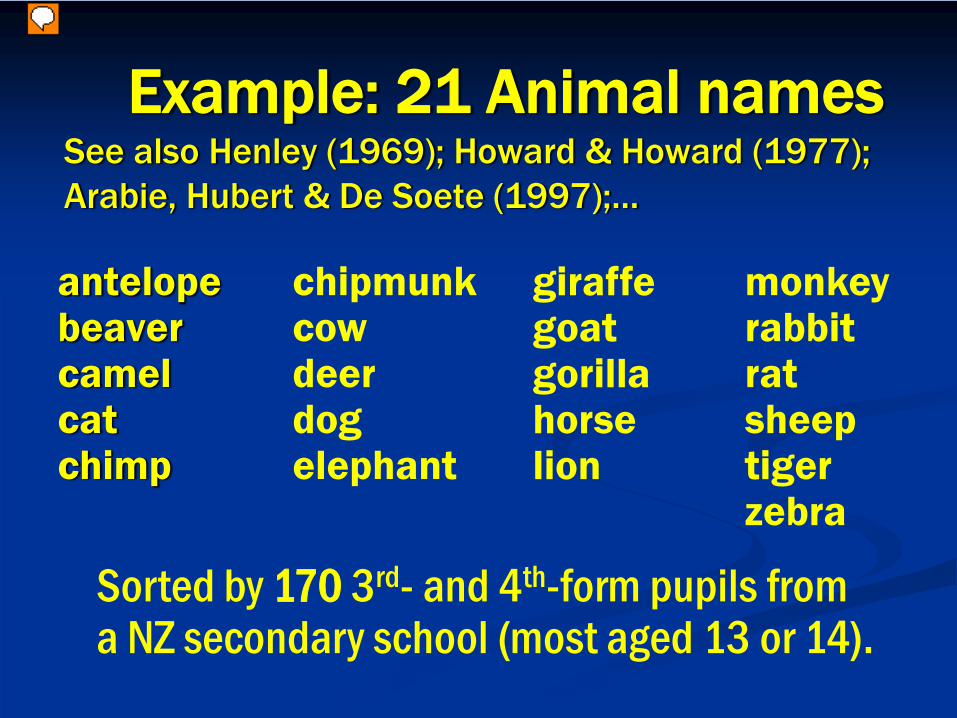
Example: 21 Animal namesSee also Henley (1969); Howard & Howard (1977); Arabie, Hubert & De Soete (1997);…

antelopebeavercamelcatchimp

chipmunkcowdeerdogelephant

monkeyrabbitratsheeptigerzebra

giraffegoatgorillahorselion

Sorted by 170 3rd- and 4th-form pupils from a NZ secondary school (most aged 13 or 14).

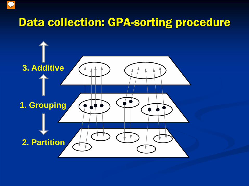
Data collection: GPA-sorting procedure

1. Grouping

2. Partition

3. Additive

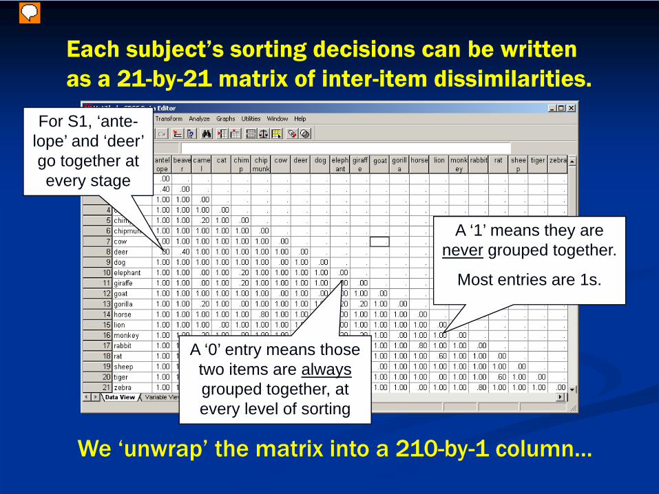
Each subject’s sorting decisions can be written as a 21-by-21 matrix of inter-item dissimilarities.

For S1, ‘ante-lope’ and ‘deer’ go together at every stage

A ‘0’ entry means those two items are alwaysgrouped together, at every level of sorting

A ‘1’ means they are never grouped together.

Most entries are 1s.

We ‘unwrap’ the matrix into a 210-by-1 column…

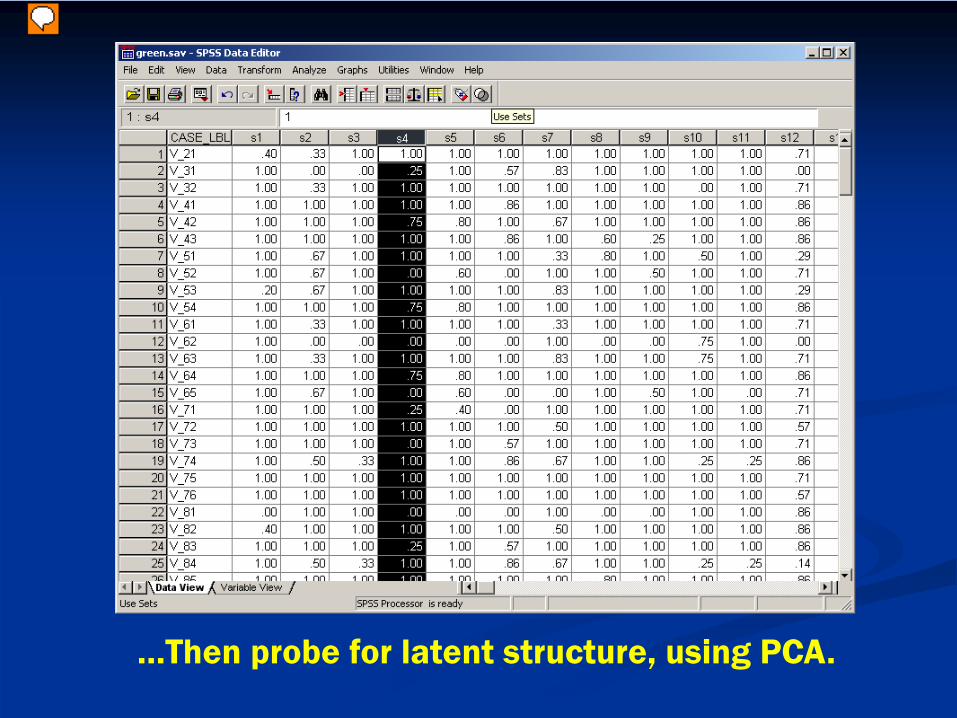
…Then probe for latent structure, using PCA.

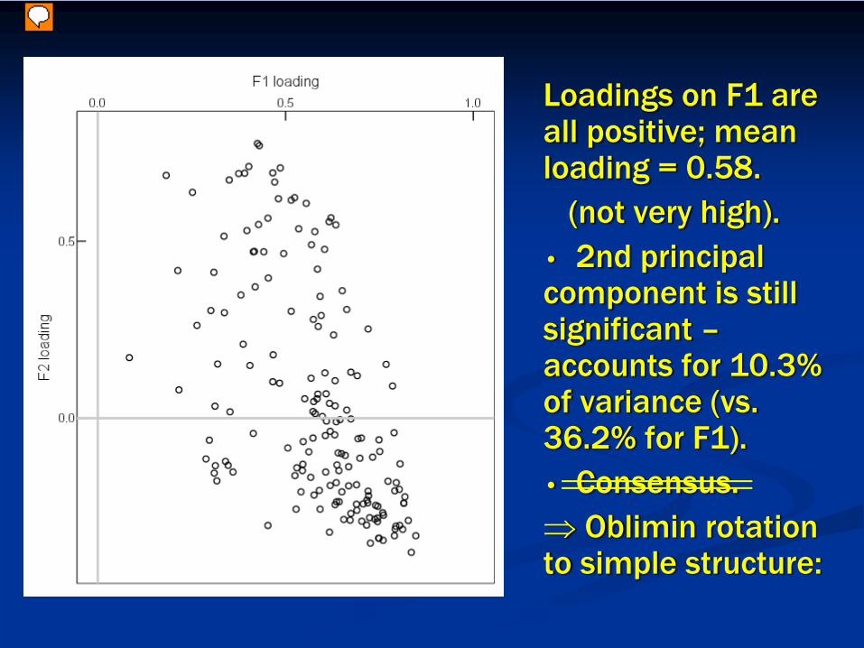
Loadings on F1 are all positive; mean loading = 0.58.

(not very high).• 2nd principal component is still significant –accounts for 10.3% of variance (vs. 36.2% for F1).• Consensus.⇒ Oblimin rotation to simple structure:

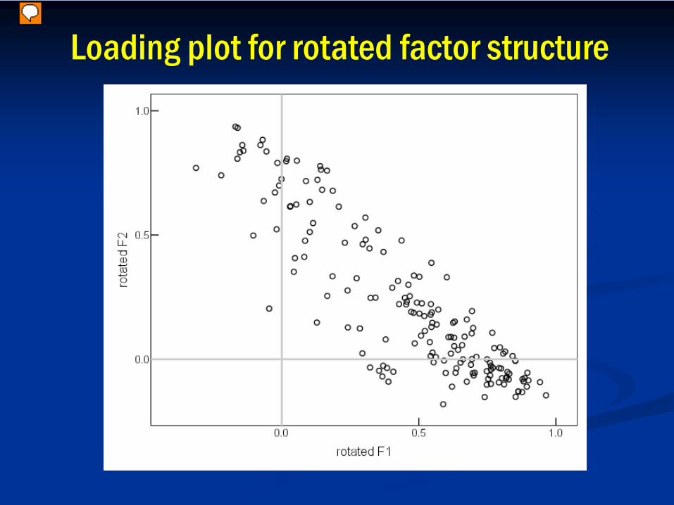
Loading plot for rotated factor structure

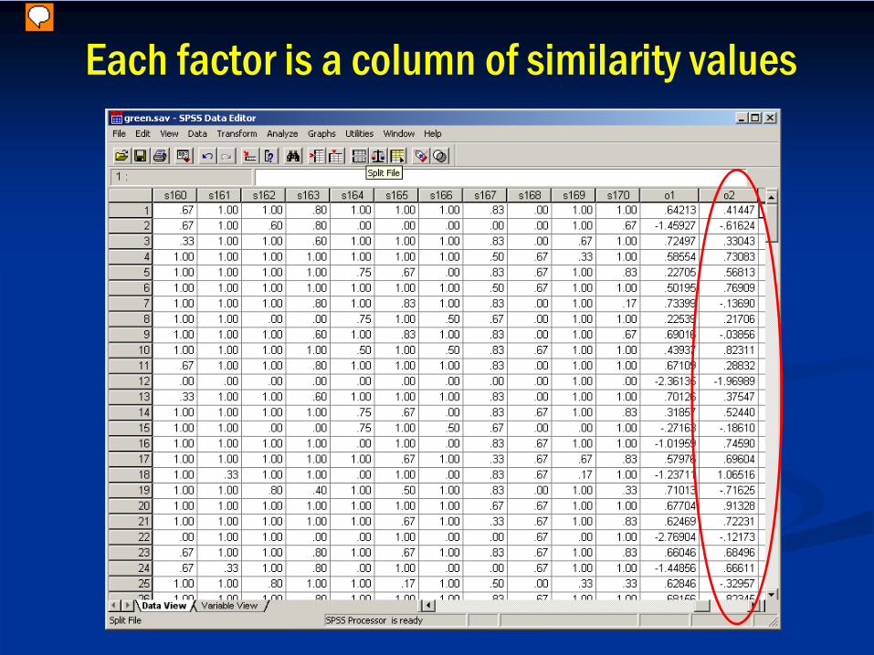
Each factor is a column of similarity values

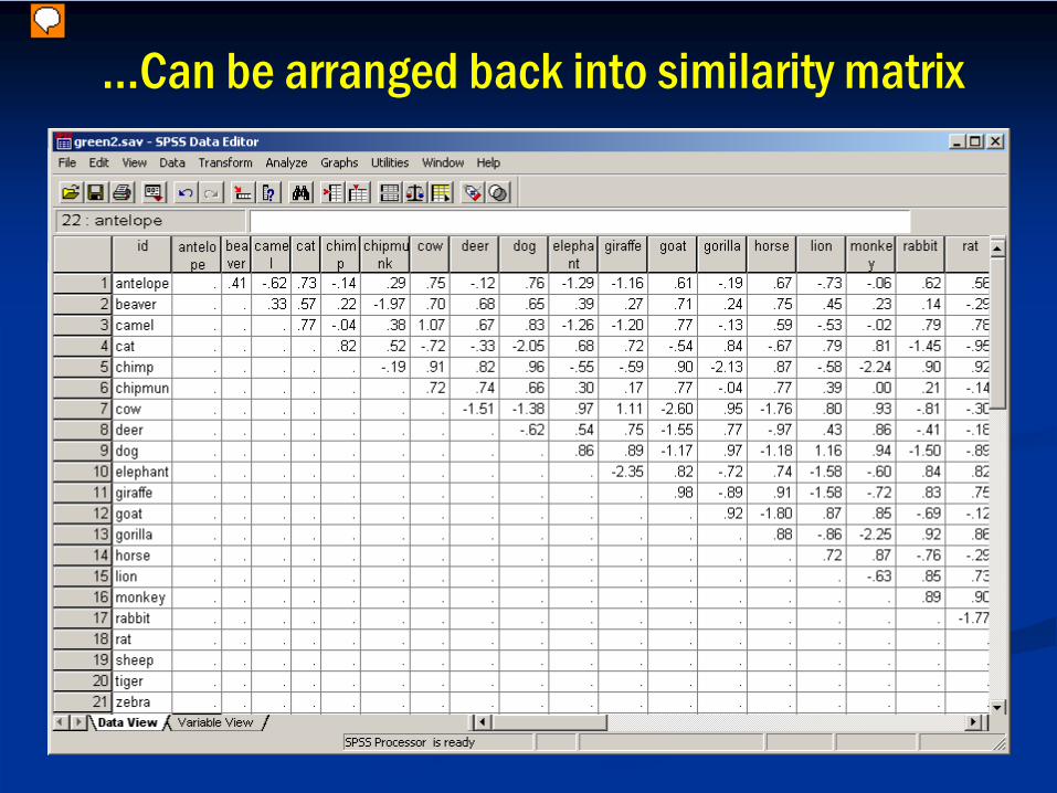
…Can be arranged back into similarity matrix

┌────────────── antelope┌───┤ ┌┬─ elephant│ │ ┌────┤└─ giraffe

┌────┤ └──────┤ └── zebra│ │ └──────┬ lion

┌───────────┤ │ └ tiger│ │ └────────────────── camel│ │

┌──────────────────────┤ └────────────────────┬── chimp│ │ ├── gorilla│ │ └── monkey│ ││ └───────────────────────────────┬─── beaver┤ └─── chipmunk││ ┌───────┬─── cat│ ┌────────┤ └─── dog│ │ └─────┬───── rabbit└─────────────────────────────────────┤ └───── rat

││ ┌───── cow│ ┌──┤┌───┬ goat└───────────┤ └┤ └ sheep

│ └──── horse└──────── deer

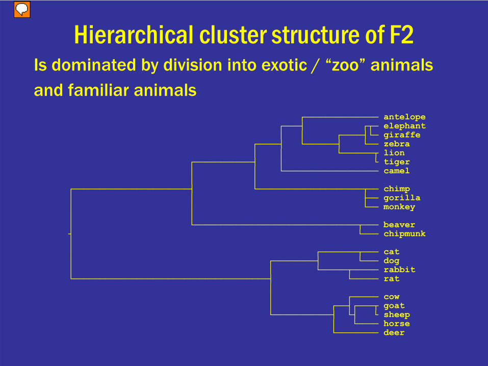
Hierarchical cluster structure of F2Is dominated by division into exotic / “zoo” animalsand familiar animals

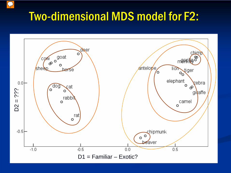
Two-dimensional MDS model for F2:

D1 = Familiar – Exotic?

D2

= ??

?

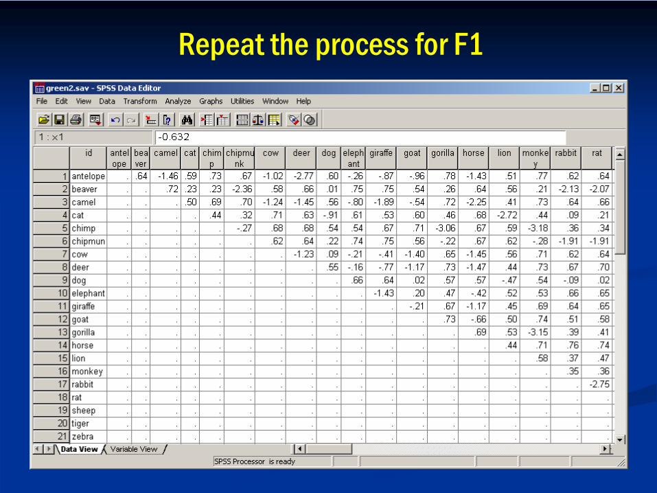
Repeat the process for F1

┌─────┬── antelope┌─────┤ └── deer│ └───┬──── camel

┌──┤ └──┬─ horse│ │ └─ zebra

┌─────────────────────────────────────┤ └─────┬──────── cow│ │ └────┬─── goat│ │ └─── sheep│ └───────┬───────── elephant│ └───────── giraffe│┤ ┌─┬─── beaver│ ┌────────────────────┤ └─── chipmunk│ ┌───────────┤ └──┬── rabbit│ │ │ └── rat│ │ ││ │ └────────────────────────┬─ chimp└────────────────┤ └┬ gorilla

│ └ monkey││ ┌─────────────┬── cat└─────────────────────┤ └─┬ lion

│ └ tiger└──────────────── dog

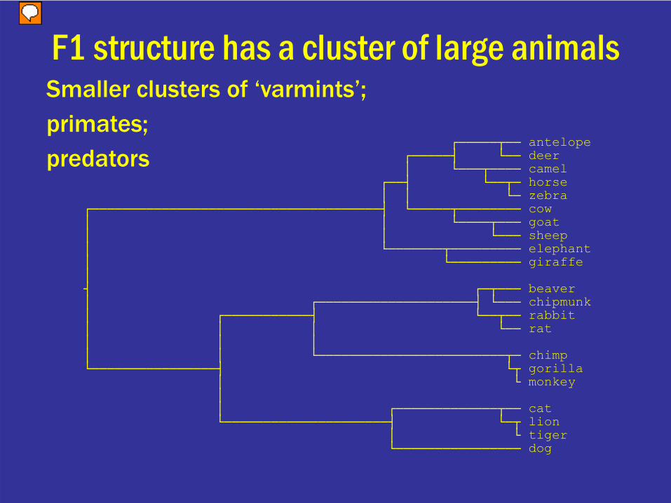
F1 structure has a cluster of large animalsSmaller clusters of ‘varmints’; primates; predators

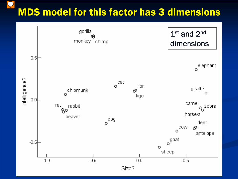
MDS model for this factor has 3 dimensions

1st and 2nd

dimensions

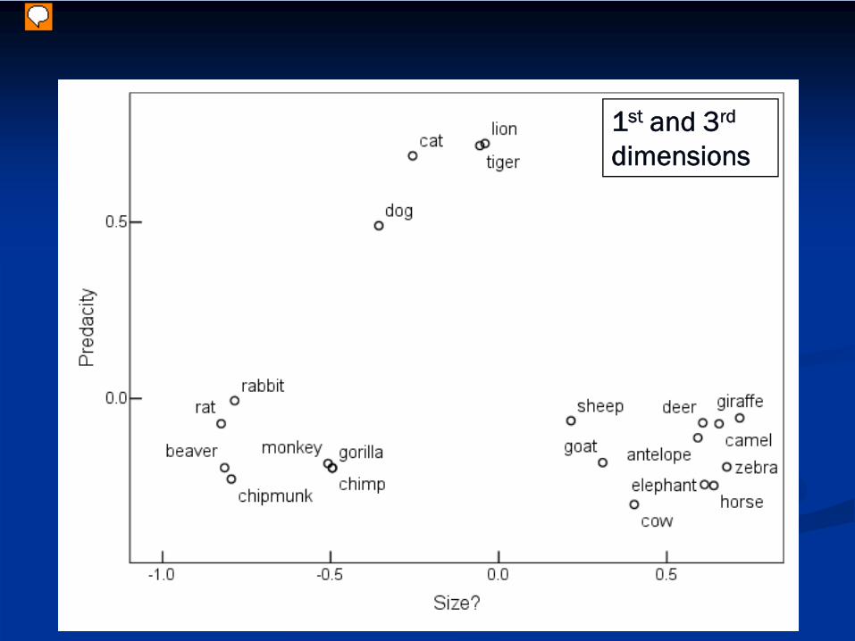
1st and 3rd

dimensions

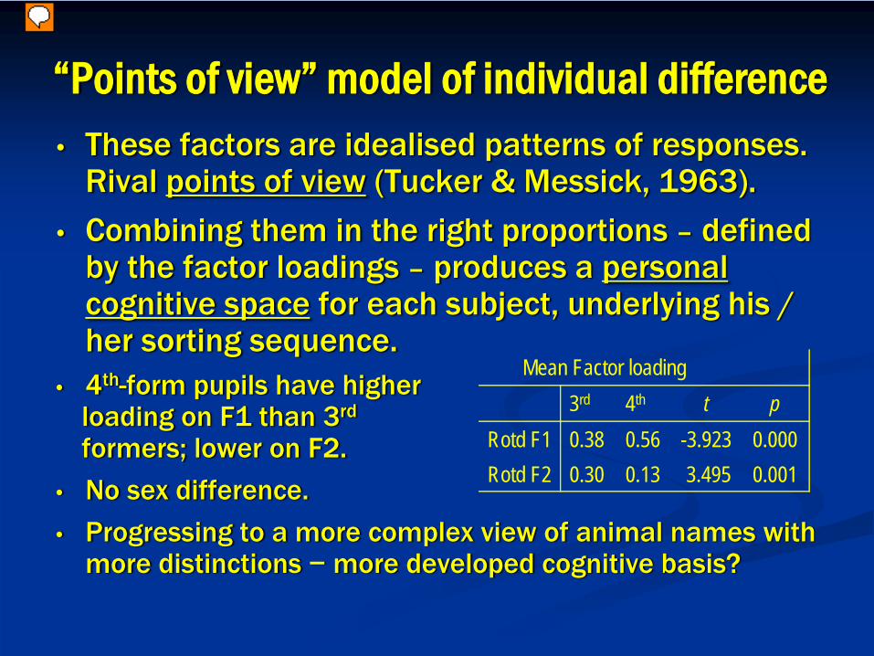
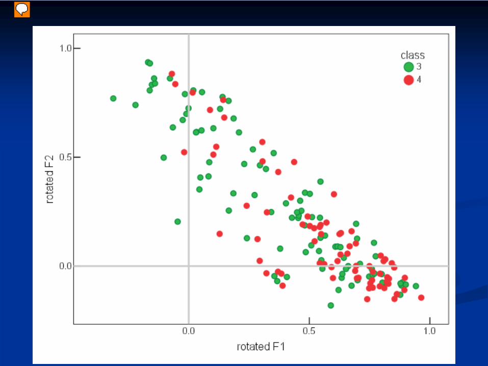
• These factors are idealised patterns of responses. Rival points of view (Tucker & Messick, 1963).

• Combining them in the right proportions – defined by the factor loadings – produces a personal cognitive space for each subject, underlying his / her sorting sequence.

• 4th-form pupils have higher loading on F1 than 3rd

formers; lower on F2.

• No sex difference.

• Progressing to a more complex view of animal names with more distinctions − more developed cognitive basis?

Mean Factor loading3rd 4th t p

Rotd F1 0.38 0.56 -3.923 0.000Rotd F2 0.30 0.13 3.495 0.001

“Points of view” model of individual difference

Presenter

Presentation Notes

Here’s the plot of individual factor loadings again, but colour-coded according to class.

• Could describe this age trend as a decrease in salience of a ‘familiarity’ axis; increase in salience of Size, Predacity, Intelligence axes.

• Would then fit within the weighted-Euclidean framework for individual variations.

• However, that requires 4 parameters to characterise each subject (vs. only two parameters for the Points-of-View model).

• Each P.o.V. is not a dimension, but a similarity structure that may contain several dimensions.

Dimension weights and “points of view”

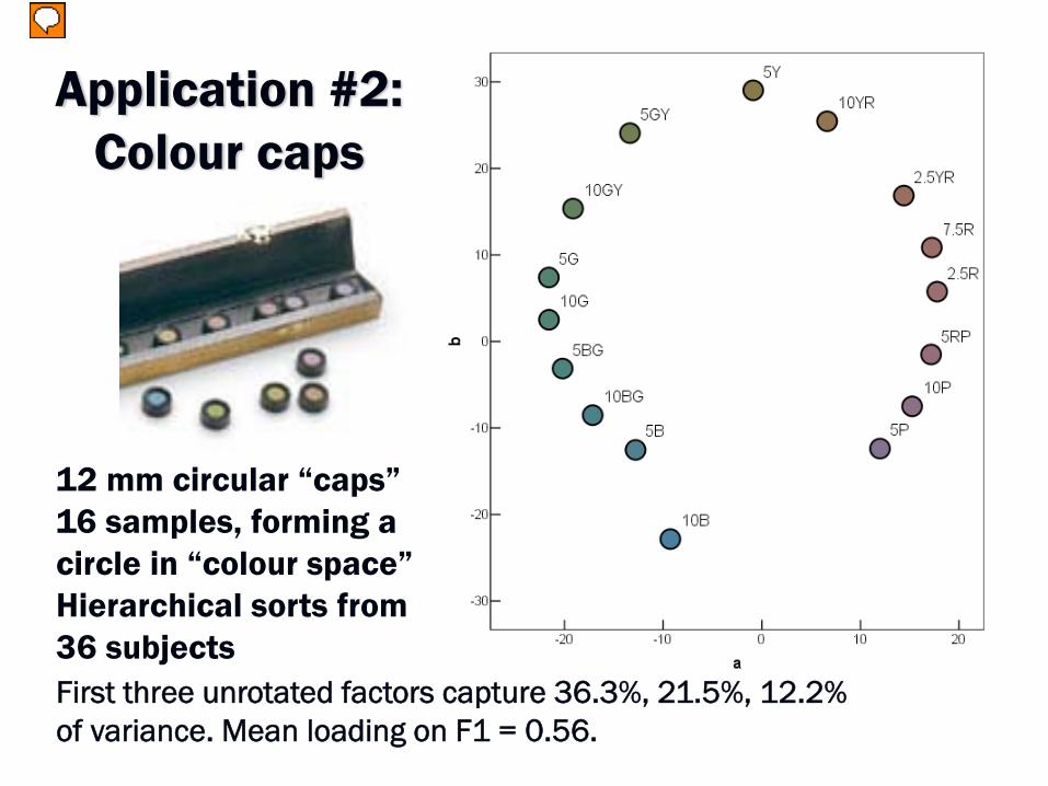
Application #2: Colour caps

First three unrotated factors capture 36.3%, 21.5%, 12.2% of variance. Mean loading on F1 = 0.56.

12 mm circular “caps”16 samples, forming a circle in “colour space”Hierarchical sorts from 36 subjects

Factor loadings after oblimin rotation

8 subjects known to be “colour blind” (red-green deficient). All high on F3.

Normal subjects polarised to F1 or F2

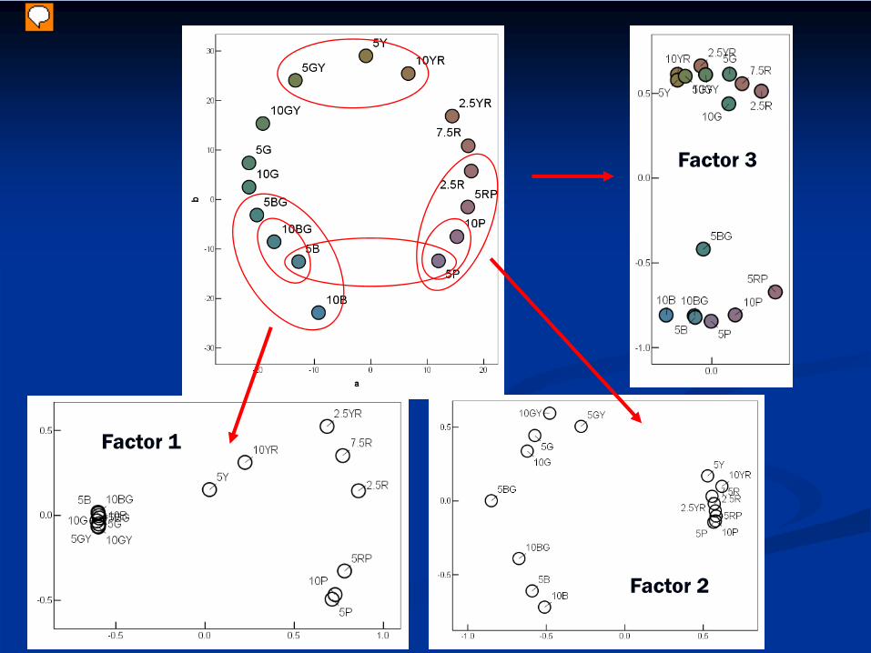
Factor 2

Factor 1

Factor 3

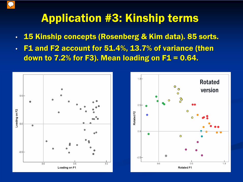
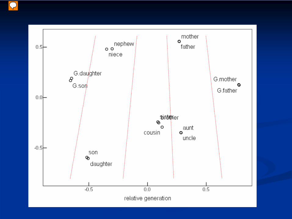
Application #3: Kinship terms• 15 Kinship concepts (Rosenberg & Kim data). 85 sorts.• F1 and F2 account for 51.4%, 13.7% of variance (then

down to 7.2% for F3). Mean loading on F1 = 0.64.

Rotated version

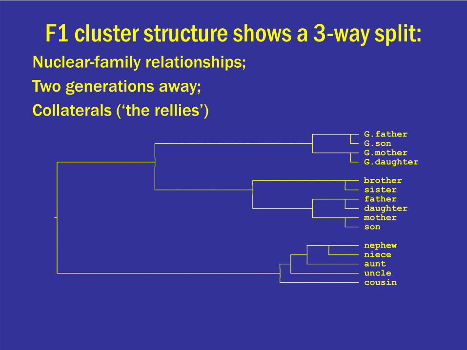
┌──────┬─ G.father┌────────────────────────────┤ └─ G.son│ └──────┬─ G.mother

┌─────────────────┤ └─ G.daughter│ ││ │ ┌────────────────┬── brother│ └─────────────────┤ └── sister│ │ ┌─────┬── father│ └──────────┤ └── daughter┤ └─────┬── mother│ └── son││ ┌───┬───── nephew│ ┌──┤ └───── niece│ ┌─┤ └───────── aunt└────────────────────────────────────────┤ └──────────── uncle

└────────────── cousin

F1 cluster structure shows a 3-way split:Nuclear-family relationships; Two generations away;Collaterals (‘the rellies’)

Presenter

Presentation Notes

MDS reveals that there is another (minor) distinction within the factor, separating males from females.

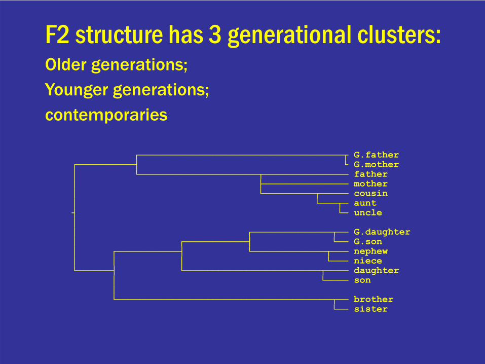
┌────────────────────────────────────┬ G.father┌──────────┤ └ G.mother│ └─────────────────────┬─────────────── father│ ├─────────────── mother│ └─────────┬───── cousin│ └───┬─ aunt┤ └─ uncle││ ┌──────────────┬── G.daughter│ ┌───────────┤ └── G.son│ ┌───────────┤ └─────────────┬─── nephew│ │ │ └─── niece└──────┤ └────────────────────────┬──── daughter

│ └──── son│└──────────────────────────────────────┬── brother

└── sister

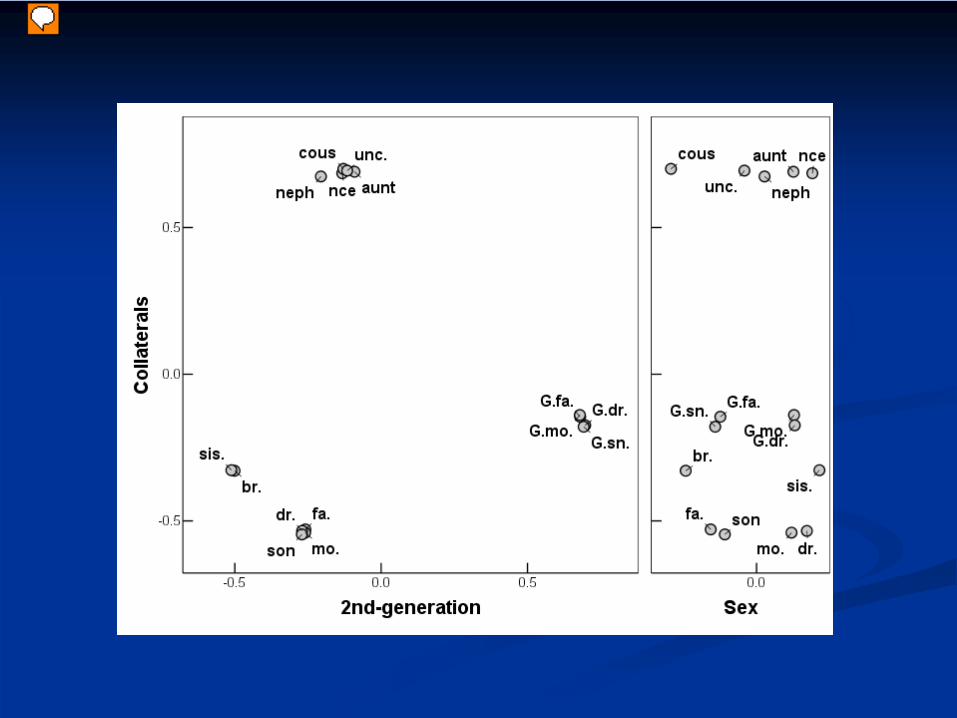
F2 structure has 3 generational clusters:Older generations; Younger generations;contemporaries

Presenter

Presentation Notes

1st dimension is ranking the kinship terms in order of generation; The 2nd dimension does not have a simple interpretation.

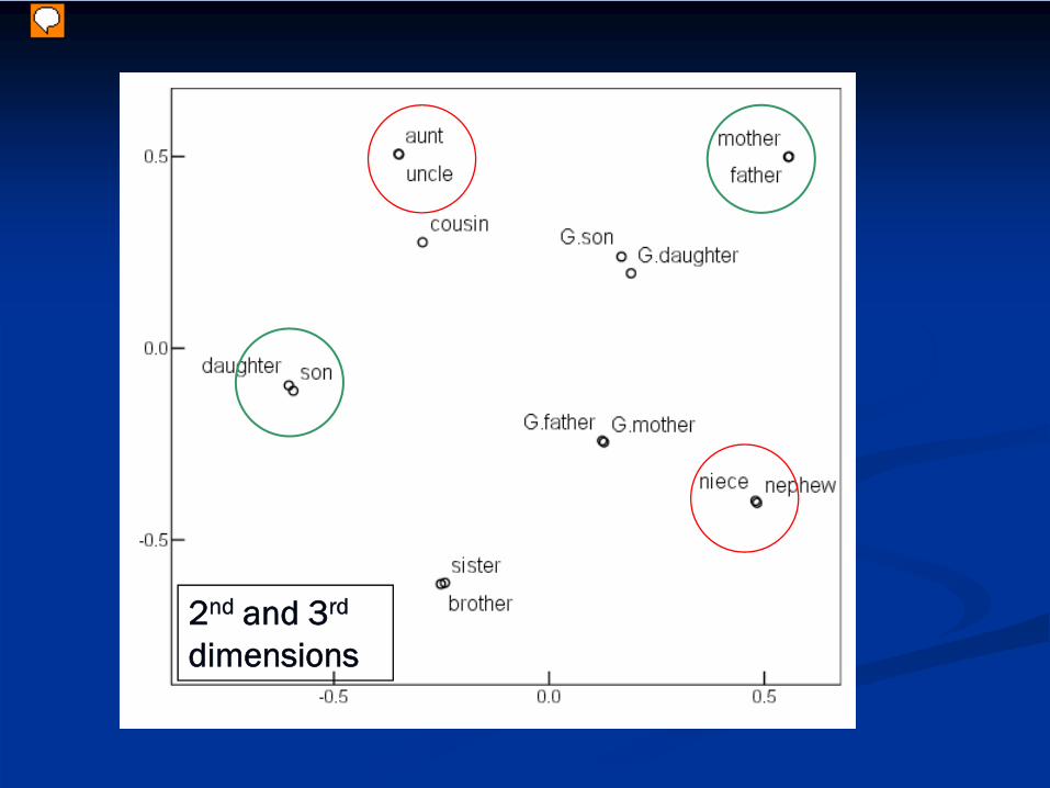
2nd and 3rd

dimensions

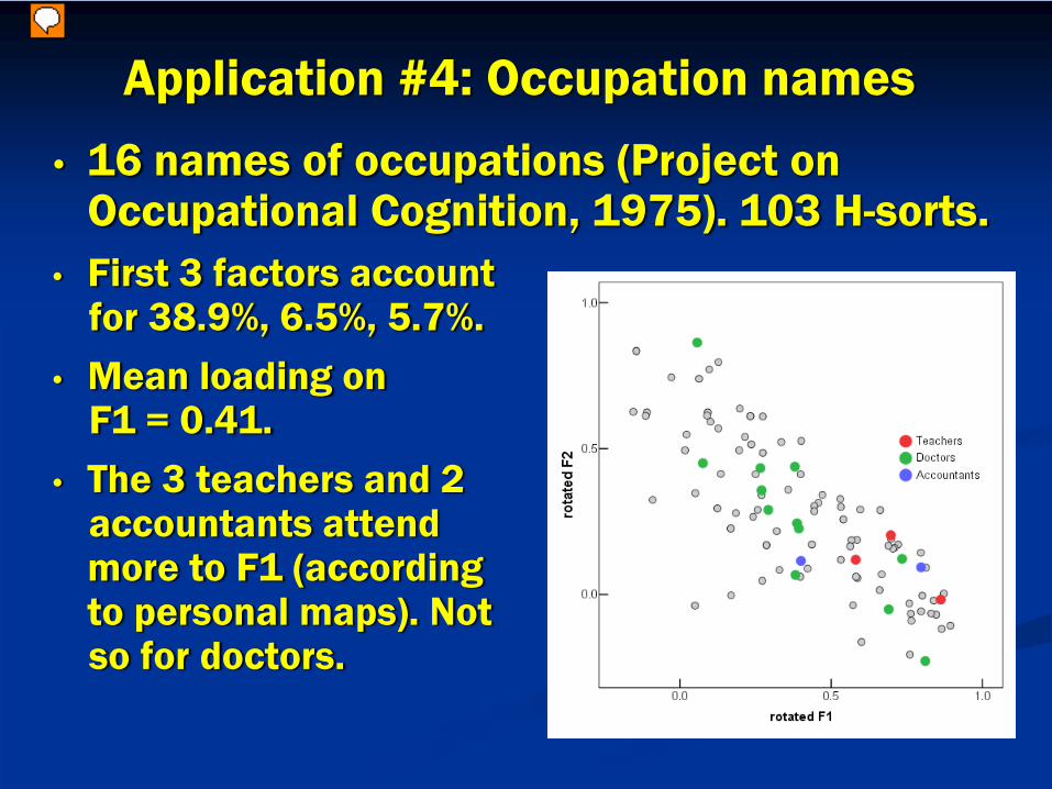
Application #4: Occupation names

• 16 names of occupations (Project on Occupational Cognition, 1975). 103 H-sorts.

• First 3 factors accountfor 38.9%, 6.5%, 5.7%.

• Mean loading on F1 = 0.41.

• The 3 teachers and 2 accountants attendmore to F1 (accordingto personal maps). Notso for doctors.

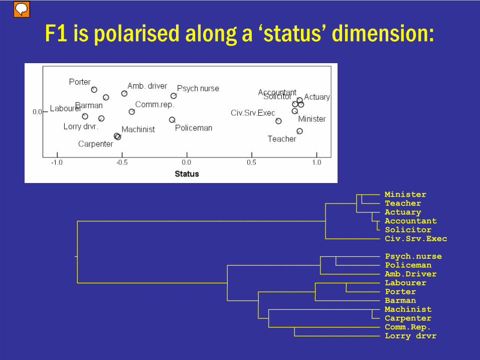
F1 is polarised along a ‘status’ dimension:

┌┬─── Minister┌─────┤└─── Teacher│ └──┬─ Actuary

┌───────────────────────────────────────────────┤ └┬ Accountant│ │ └ Solicitor│ └────────── Civ.Srv.Exec│┤ ┌──┬──────── Psych.nurse│ ┌─────────────────┤ └──────── Policeman│ │ └─────────── Amb.Driver└────────────────────────────┤ ┌─────┬────── Labourer

│ ┌──────────┤ └────── Porter└─────┤ └──────────── Barman

│ ┌───────────────────┬─ Machinist└─┤ └─ Carpenter└────┬──────────────── Comm.Rep.

└──────────────── Lorry drvr

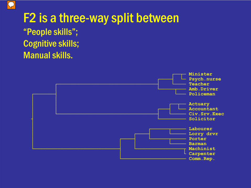
F2 is a three-way split between“People skills”;Cognitive skills;Manual skills.

┌──┬─ Minister┌────┤ └─ Psych.nurse

┌──────────────────────────────────┤ └──── Teacher│ └─────┬─── Amb.Driver

┌───────┤ └─── Policeman│ ││ │ ┌──┬── Actuary│ │ ┌───┤ └── Accountant│ └──────────────────────────────────┤ └───── Civ.Srv.Exec┤ └───────── Solicitor││ ┌──────┬───── Labourer│ ┌────┤ └───── Lorry drvr│ ┌────┤ └──────┬───── Porter│ │ │ └───── Barman└─────────────────────────────┤ └────────────────┬ Machinist

│ └ Carpenter└────────────────────── Comm.Rep.

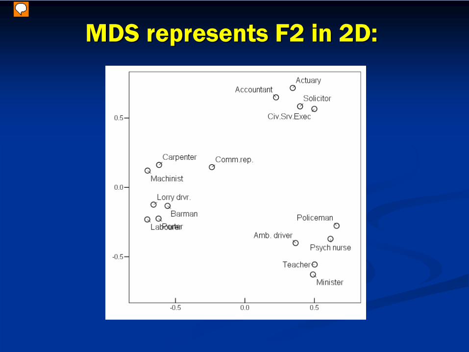
MDS represents F2 in 2D:

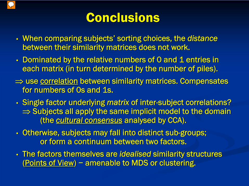
Conclusions• When comparing subjects’ sorting choices, the distance

between their similarity matrices does not work.

• Dominated by the relative numbers of 0 and 1 entries in each matrix (in turn determined by the number of piles).

⇒ use correlation between similarity matrices. Compensates for numbers of 0s and 1s.

• Single factor underlying matrix of inter-subject correlations? ⇒ Subjects all apply the same implicit model to the domain

(the cultural consensus analysed by CCA).

• Otherwise, subjects may fall into distinct sub-groups; or form a continuum between two factors.

• The factors themselves are idealised similarity structures (Points of View) − amenable to MDS or clustering.

Thank you

• Acknowledgements to the Project on Occupational Cognition, which conducted the hierarchical sorting of job titles,

• And the UK Data Service at the University of Essex, who are the custodians of the data.

• Emma Barraclough helped collect the colour data.

• Enormous debt to A. P. M. Coxon for delivering talk.