subset selection problem oxana rodionova & alexey pomerantsev semenov institute of chemical...

Subset Selection ProblemSubset Selection Problem

Oxana Rodionova & Alexey Pomerantsev

Semenov Institute of Chemical Physics Russian Chemometric Society

Moscow

OutlineOutline

Introduction. What is representative subset ?

Training set and Test set

Influential subset selection

Boundary subset

Kennard-Stone subset

Models’ comparison

Conclusions

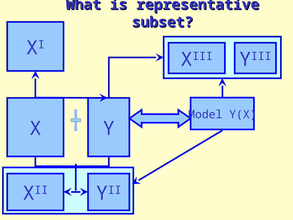
What is representative subset?What is representative subset?

YX

XI

Model Y(X)

XII YII

XIII YIII

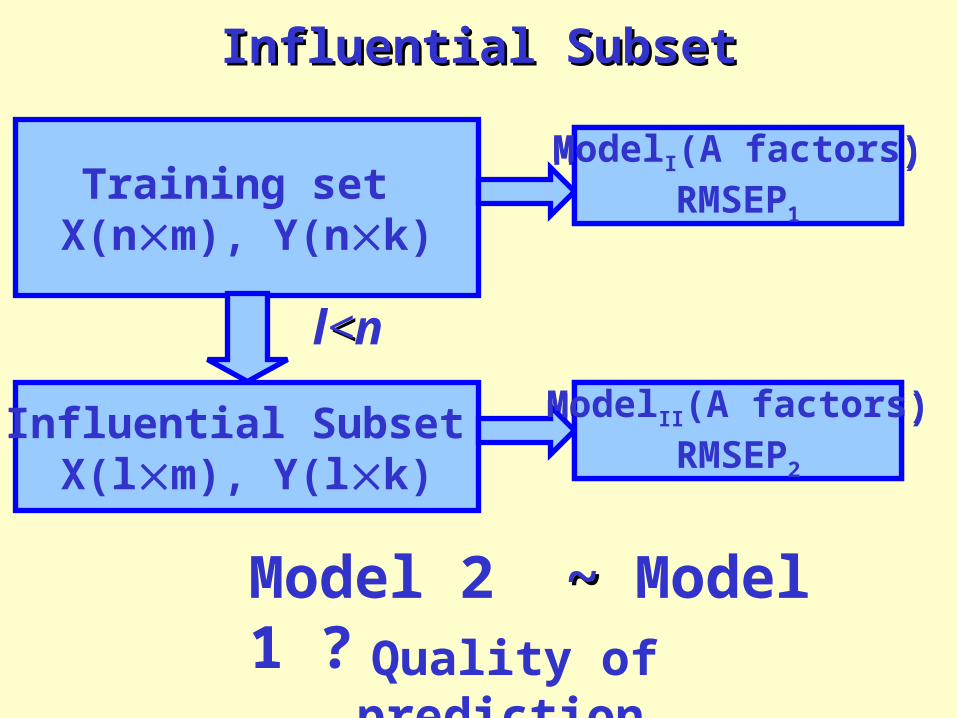
Influential SubsetInfluential Subset

Training set X(nm), Y(nk)

Influential Subset X(lm), Y(lk)

ModelI(A factors)

ModelII(A factors)

l<<n

Model 2 ~ ~ Model 1 ?

ModelI(A factors)RMSEP1

ModelII(A factors)RMSEP2

Quality of prediction

Training and Test SetsTraining and Test Sets

Entire Data SetK

Entire Data SetK

Training SetN

Training SetN

Test SetK-N

Test SetK-N

-25

-20

-15

-10

-5

0

5

10

15

20

-15 -10 -5 0 5 10 15

X1

X2

-25

-20

-15

-10

-5

0

5

10

15

20

-15 -10 -5 0 5 10 15

X1

X2

-25

-20

-15

-10

-5

0

5

10

15

20

-15 -10 -5 0 5 10 15

X1

X2

-25

-20

-15

-10

-5

0

5

10

15

20

-15 -10 -5 0 5 10 15

X1

X2

-25

-20

-15

-10

-5

0

5

10

15

20

-15 -10 -5 0 5 10 15

X1

X2

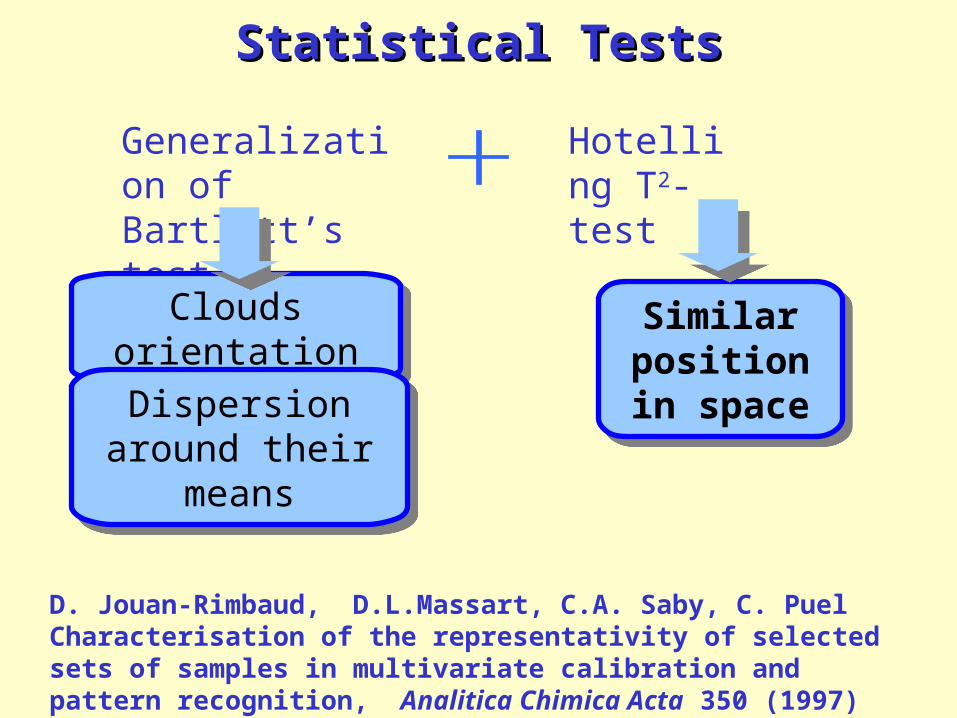
Statistical TestsStatistical Tests

D. Jouan-Rimbaud, D.L.Massart, C.A. Saby, C. Puel Characterisation of the representativity of selected sets of samples in multivariate calibration and pattern recognition, Analitica Chimica Acta 350 (1997) 149-161

Generalization of Bartlett’s test

Hotelling T2-test

Clouds orientationClouds orientation

Dispersion around their means

Dispersion around their means

Similar position in

space

Similar position in

space

24

232221

20

19

18

1716

15

14

13

12

11

10

9

8

7

6

5

4

3

2

1

-1

0

1

0 1

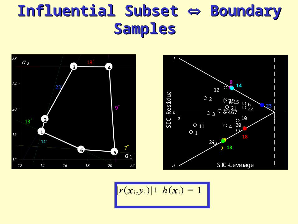
SIC-LeverageSIC-Residual

18+

9–

14–

13+

7+

23–

1

2

3

6 5

4

1

12

16

20

24

28

12 14 16 18 20 22

a 1

a 2 18+

9–

14–

13+

7+

23–

1

2

3

6 5

4

1

12

16

20

24

28

12 14 16 18 20 22

a 1

a 2

RPV

Influential Subset Influential Subset Boundary Samples Boundary Samples

Whole Wheat Samples(Data description)

X- NIR Spectra of Whole Wheat (118 wave lengths)

Y- moisture content

N=139 Entire Set

Data pre- processed.

X- NIR Spectra of Whole Wheat (118 wave lengths)

Y- moisture content

N=139 Entire Set

Data pre- processed.

PLS-model, 4PCs

SIC-modeling bsic=1.5

PLS-model, 4PCs

SIC-modeling bsic=1.5

Training set = 99 objects

Test set = 40 objects

Training set = 99 objects

Test set = 40 objects

C Ccrit

12 18

F Fcrit

1 2.4

C Ccrit

12 18

F Fcrit

1 2.4

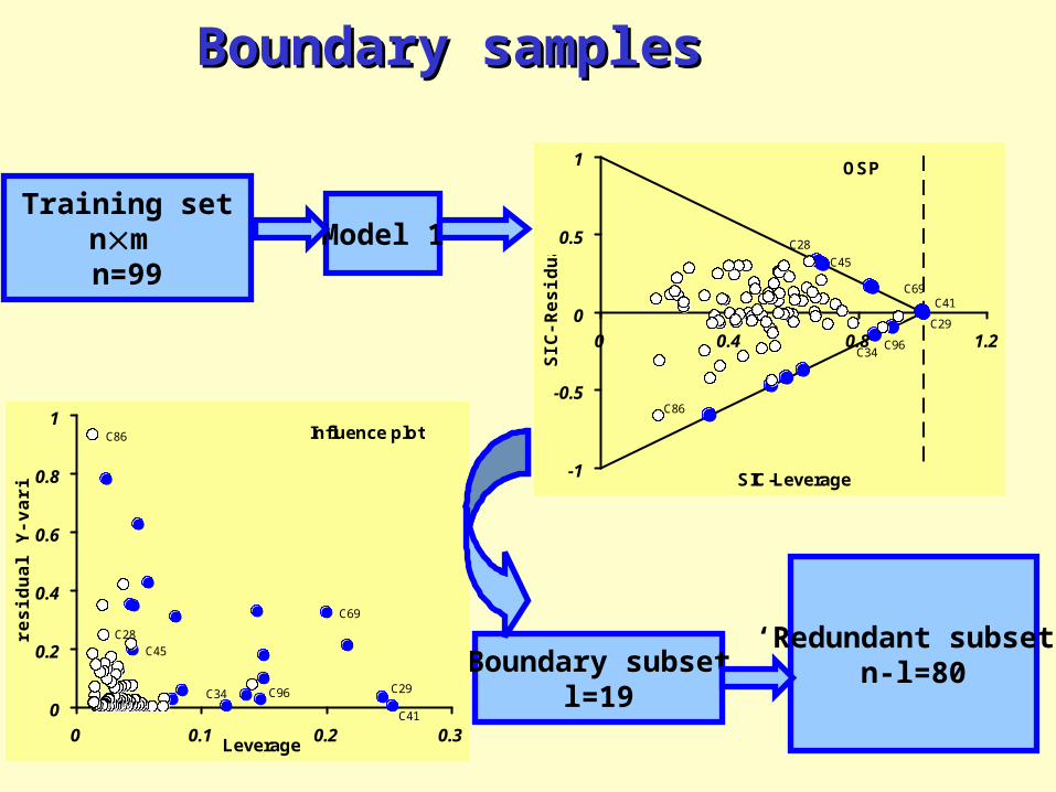
Boundary subsetl=19

Influence plot

C45

C34

C41

C29

C69

C28

C96

C86

0

0.2

0.4

0.6

0.8

1

0 0.1 0.2 0.3Leverage

res

idu

al Y

-va

ria

nc

e

Boundary samplesBoundary samples

Training setnm n=99

Model 1

‘Redundant subset’n-l=80

OSP

C34

C41C69

C45

C86

C96

C29

C28

-1

-0.5

0

0.5

1

0 0.4 0.8 1.2

SIC-Leverage

SIC

-Re

sid

ua

l

`

Boundary Subset Boundary Subset

Training setModel 1

Training setModel 1

Boundary subsetModel 2


TEST SETTEST SETn=99 l=19

4 PLS comp-s=1.5

Callibration/Test

40

3938

3736

35

34

33

32

3130

29

28

27

26

25 2423 2221

20 19

18

1716

1514

1312

1110

9

8

76

5

4

3

2

1

-1

-0.8

-0.6

-0.4

-0.2

0

0.2

0.4

0.6

0.8

1

0 0.2 0.4 0.6 0.8 1 1.2

SIC-Leverage

SIC

-Res

idu

al

Boundary/Test

40

3938

37 36

35

34

33

32

3130

29

28

27

26

25 2423 2221

20 19

18

1716

1514

1312

1110

9

8

76

5

4

3

2

1

-1

-0.8

-0.6

-0.4

-0.2

0

0.2

0.4

0.6

0.8

1

0 0.2 0.4 0.6 0.8 1 1.2

SIC-Leverage

SIC

-Res

idu

al

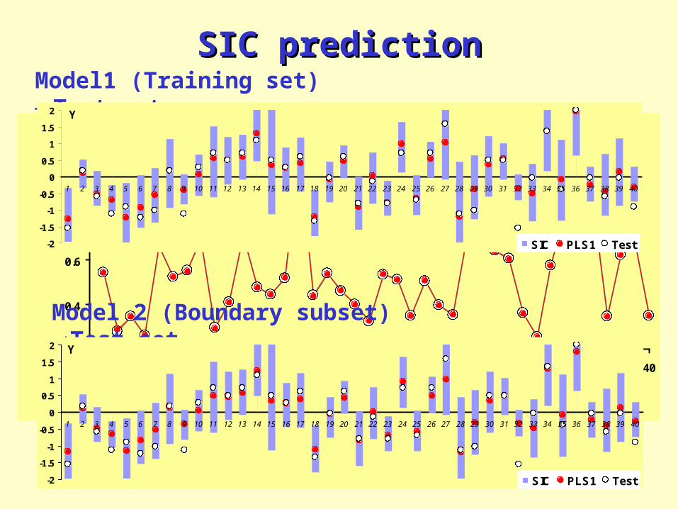
SIC predictionSIC prediction

0.2

0.4

0.6

0.8

1

1.2

0 5 10 15 20 25 30 35 40

Sample #

SIC

lev

era

ge

Training Boundary

Model1 (Training set) Test set

Model 2 (Boundary subset) Test set

-2

-1.5

-1

-0.5

0

0.5

1

1.5

2

1 2 3 4 5 6 7 8 9 10 11 12 13 14 15 16 17 18 19 20 21 22 23 24 25 26 27 28 29 30 31 32 33 34 35 36 37 38 39 40

Y

SIC PLS1 Test

-2

-1.5

-1

-0.5

0

0.5

1

1.5

2

1 2 3 4 5 6 7 8 9 10 11 12 13 14 15 16 17 18 19 20 21 22 23 24 25 26 27 28 29 30 31 32 33 34 35 36 37 38 39 40

Y

SIC PLS1 Test

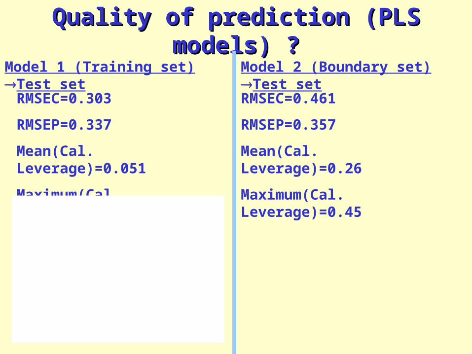
Quality of prediction (PLS models) ?Quality of prediction (PLS models) ?

RMSEC=0.303

RMSEP=0.337

Mean(Cal. Leverage)=0.051

Maximum(Cal. Leverage)=0.25

RMSEC=0.461

RMSEP=0.357



Model 1 (Training set) Test set Model 2 (Boundary set) Test set

Model1

0

0.1

0.2

0.3

0.4

0.5

0 20 40 60 80 100 120 140

Sample #

Y le

vera

ge

Model 2

27

28

15

2932

0

0.1

0.2

0.3

0.4

0.5

0 10 20 30 40 50 60Sample #

Y le

vera

ge

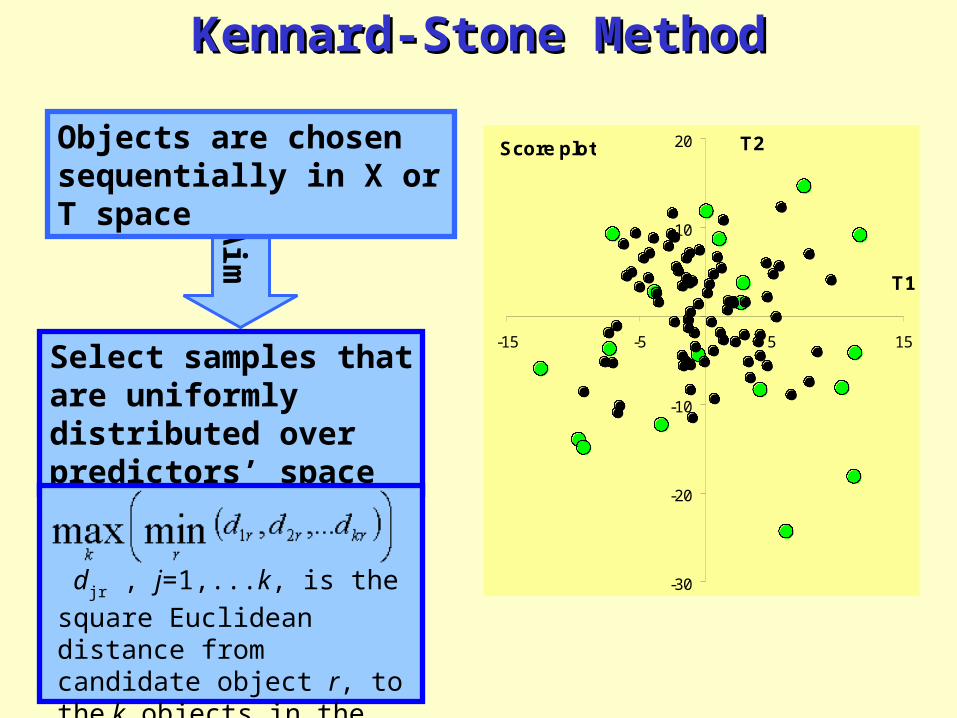
Aim

Score plot

-30

-20

-10

0

10

20

-15 -10 -5 0 5 10 15

T1

T2

Kennard-Stone MethodKennard-Stone Method

Objects are chosen sequentially in X or T space

Select samples that are uniformly distributed over predictors’ space

djr , j=1,...k, is the square

Euclidean distance from candidate object r, to the k objects in the subset

Score plot

-30

-20

-10

0

10

20

-15 -5 5 15

T1

T2

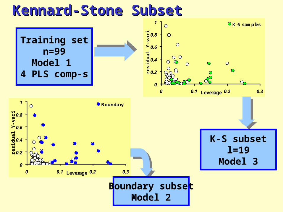
Kennard-Stone SubsetKennard-Stone Subset

0

0.2

0.4

0.6

0.8

1

0 0.1 0.2 0.3Leverage

res

idu

al Y

-va

ria

nc

e

K-S samples

0

0.2

0.4

0.6

0.8

1

0 0.1 0.2 0.3Leverage

res

idu

al Y

-va

ria

nc

e

Boundary

Training setn=99

Model 1 4 PLS comp-s

K-S subsetl=19

Model 3


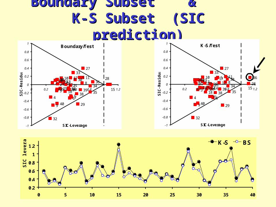
Boundary Subset & K-S Subset Boundary Subset & K-S Subset (SIC prediction)(SIC prediction)

K-S/Test

40

3938

3736

35

34

33

32

3130

29

28

27

26

252423 2221

2019

18

1716

1514

13 12

1110

9

8

7 6

5

4

3

2

1

-1

-0.8

-0.6

-0.4

-0.2

0

0.2

0.4

0.6

0.8

1

0 0.2 0.4 0.6 0.8 1 1.2

SIC-Leverage

SIC

-Res

idu

al

0.2

0.4

0.6

0.8

1

1.2

0 5 10 15 20 25 30 35 40

SIC

lev

era

ge K-S BS

Boundary/Test

1

2

3

4

5

67

8

9

10 11

1213

14 15

1617

18

1920212223 2425

26

27

28

29

3031

32

33

34

35

3637

3839

40

-1

-0.8

-0.6

-0.4

-0.2

0

0.2

0.4

0.6

0.8

1

0 0.2 0.4 0.6 0.8 1 1.2

SIC-Leverage

SIC

-Res

idu

al

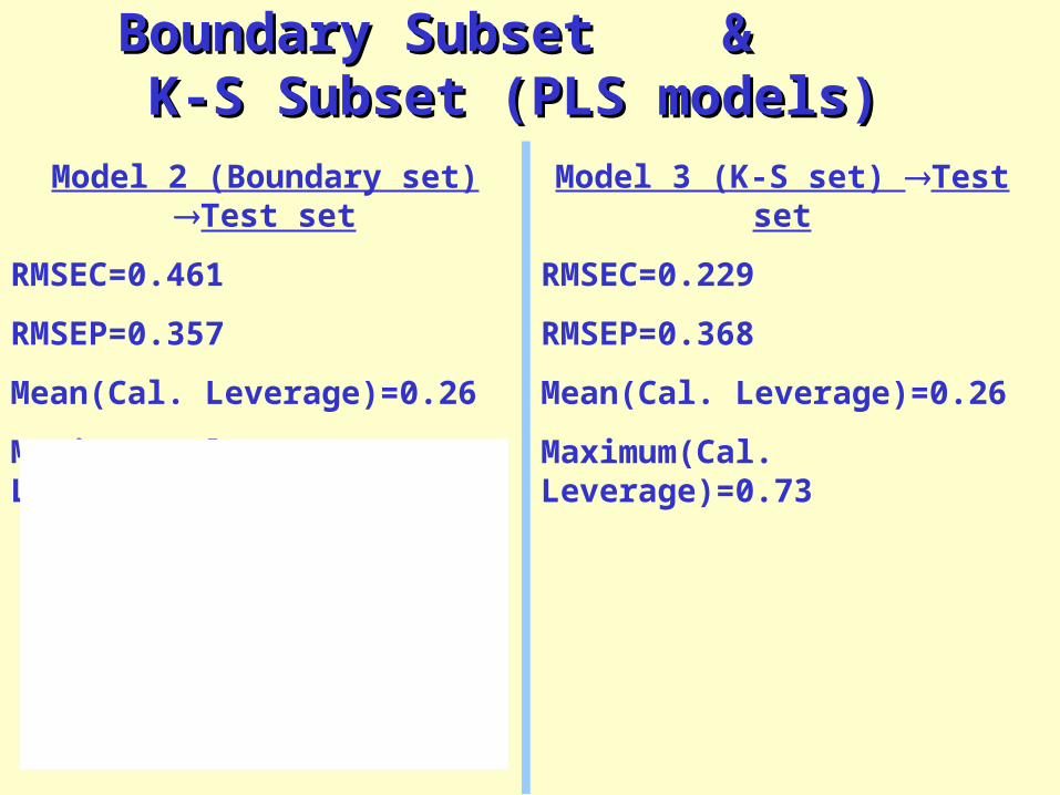
Boundary Subset & K-S Subset Boundary Subset & K-S Subset (PLS models) (PLS models)

Model 2 (Boundary set) Test set

RMSEC=0.461

RMSEP=0.357



Model 3 (K-S set) Test set

RMSEC=0.229

RMSEP=0.368



Model 2

3229

15

28

27

0

0.1

0.2

0.3

0.4

0.5

0.6

0.7

0.8

0 10 20 30 40 50 60Sample #

Y le

vera

ge

Model 3

15

28

0

0.1

0.2

0.3

0.4

0.5

0.6

0.7

0.8

0 10 20 30 40 50 60Sample #

Y le

vera

ge

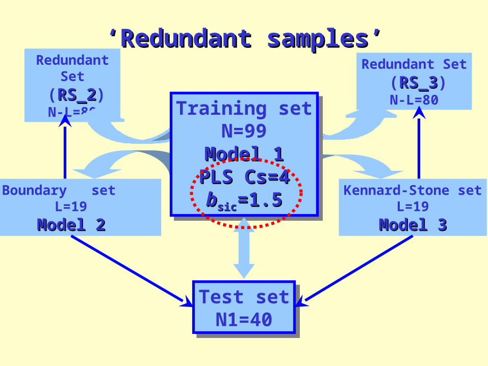
‘‘Redundant samples’Redundant samples’

Kennard-Stone setL=19

Model 3Model 3

Redundant Set

(RS_3RS_3)N-L=80

Boundary set L=19

Model 2Model 2

Redundant Set

(RS_2RS_2)N-L=80

Test setN1=40

Test setN1=40

Training setN=99

Model 1Model 1PLS Cs=4PLS Cs=4

bbsicsic=1.5=1.5

Training setN=99

Model 1Model 1PLS Cs=4PLS Cs=4

bbsicsic=1.5=1.5

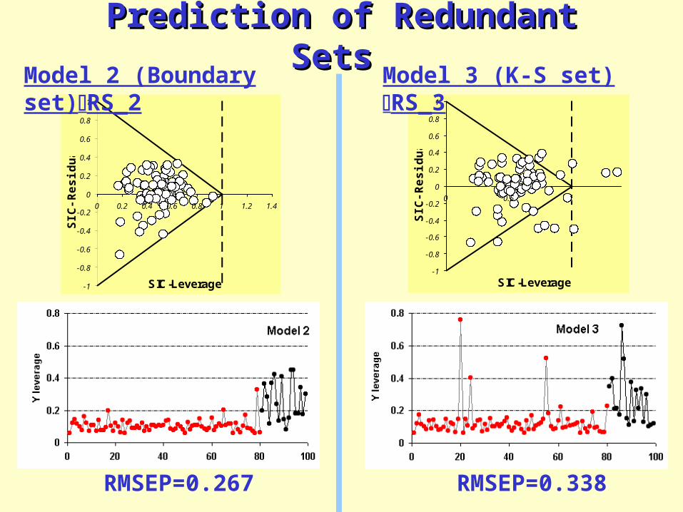
Prediction of Redundant Sets Prediction of Redundant Sets

-1

-0.8

-0.6

-0.4

-0.2

0

0.2

0.4

0.6

0.8

1

0 0.2 0.4 0.6 0.8 1 1.2 1.4

SIC-Leverage

SIC

-Re

sid

ua

l

-1

-0.8

-0.6

-0.4

-0.2

0

0.2

0.4

0.6

0.8

1

0 0.5 1

SIC-Leverage

SIC

-Re

sid

ua

l

Model 2 (Boundary set)RS_2 Model 3 (K-S set) RS_3

RMSEP=0.267 RMSEP=0.338

Model comparisonModel comparison

Entire Data Set139 objects

Training Set99 objects

Test Set40 objects

Randomly 10 times

In Average

Kenn.-Stone SetBoundary SetTraning Set0

0.1

0.2

0.3

0.4RMSEC RMSEP

ConclusionsConclusions

1. The model constructed with the help of Boundary Subset can predict all other samples with accuracy that is not worse than the error of calibration evaluated on the whole data set.

2. Boundary Subset is indeed significantly smaller than the whole Training Set.

QuestionsQuestions

1. Prediction ability, how to evaluate it? 2. Representativity, how to verify it?

subset selection problem oxana rodionova & alexey pomerantsev semenov institute of chemical...

Documents