Subspace Alignment For Domain Adaptation

Basura Fernando1, Amaury Habrard2, Marc Sebban2, and Tinne Tuytelaars1

1KU Leuven, ESAT-PSI, iMinds, Belgium2Universite de Lyon, Universite de St-Etienne F-42000, , UMR CNRS 5516, Laboratoire

Hubert-Curien, France

AbstractIn this paper, we introduce a new domain adaptation(DA) algorithm where the source and target domainsare represented by subspaces spanned by eigenvectors.Our method seeks a domain invariant feature space bylearning a mapping function which aligns the sourcesubspace with the target one. We show that the solutionof the corresponding optimization problem can be ob-tained in a simple closed form, leading to an extremelyfast algorithm. We present two approaches to determinethe only hyper-parameter in our method correspondingto the size of the subspaces. In the first approach wetune the size of subspaces using a theoretical bound onthe stability of the obtained result. In the second ap-proach, we use maximum likelihood estimation to de-termine the subspace size, which is particularly usefulfor high dimensional data. Apart from PCA, we pro-pose a subspace creation method that outperform par-tial least squares (PLS) and linear discriminant analysis(LDA) in domain adaptation. We test our method onvarious datasets and show that, despite its intrinsic sim-plicity, it outperforms state of the art DA methods.

1 IntroductionIn classification, it is typically assumed that the test datacomes from the same distribution as that of the labeledtraining data. However, many real world applications,especially in computer vision, challenge this assump-tion (see, e.g., the study on dataset bias in [26]). Inthis context, the learner must take special care duringthe learning process to infer models that adapt well tothe test data they are deployed on. For example, im-ages collected from a DSLR camera are different fromthose taken with a web camera. A classifier that istrained on the former would likely fail to classify the

latter correctly if applied without adaptation. Likewise,in face recognition the objective is to identify a per-son using available training images. However, the testimages may arise from very different capturing condi-tions than the ones in the training set. In image anno-tation, the training images (such as ImageNet) could bevery different from the images that we need to annotate(for example key frames extracted from an old video).These are some examples where training and test dataare drawn from different distributions.

We refer to these different but related joint distribu-tions as domains. Formally, if we denote P(χd) as thedata distribution and P(ϑd) the label distribution of do-main d, then the source domain S and the target do-main T have different joint distributions P(χS,ϑS) 6=P(χT ,ϑT ). In order to build robust classifiers, it is thusnecessary to take into account the shift between thesetwo distributions. Methods that are designed to over-come this shift in domains are known as domain adap-tation (DA) methods. DA typically aims at making useof information coming from both source and target do-mains during the learning process to adapt automati-cally. One usually differentiates between two scenar-ios: (1) the unsupervised setting where the training con-sists of labeled source data and unlabeled target exam-ples (see [19] for a survey); and (2) the semi-supervisedcase where a large number of labels are available forthe source domain and only a few labels are providedfor the target domain. In this paper, we focus on themost difficult, unsupervised scenario.

As illustrated by recent results [12, 13], subspacebased domain adaptation seems to be a promising ap-proach to tackle unsupervised visual DA problems. In[13], Gopalan et al. generate intermediate representa-tions in the form of subspaces along the geodesic pathconnecting the source subspace and the target subspaceon the Grassmann manifold. Then, the source data

1

arX

iv:1

409.

5241

v2 [

cs.C

V]

23

Oct

201

4

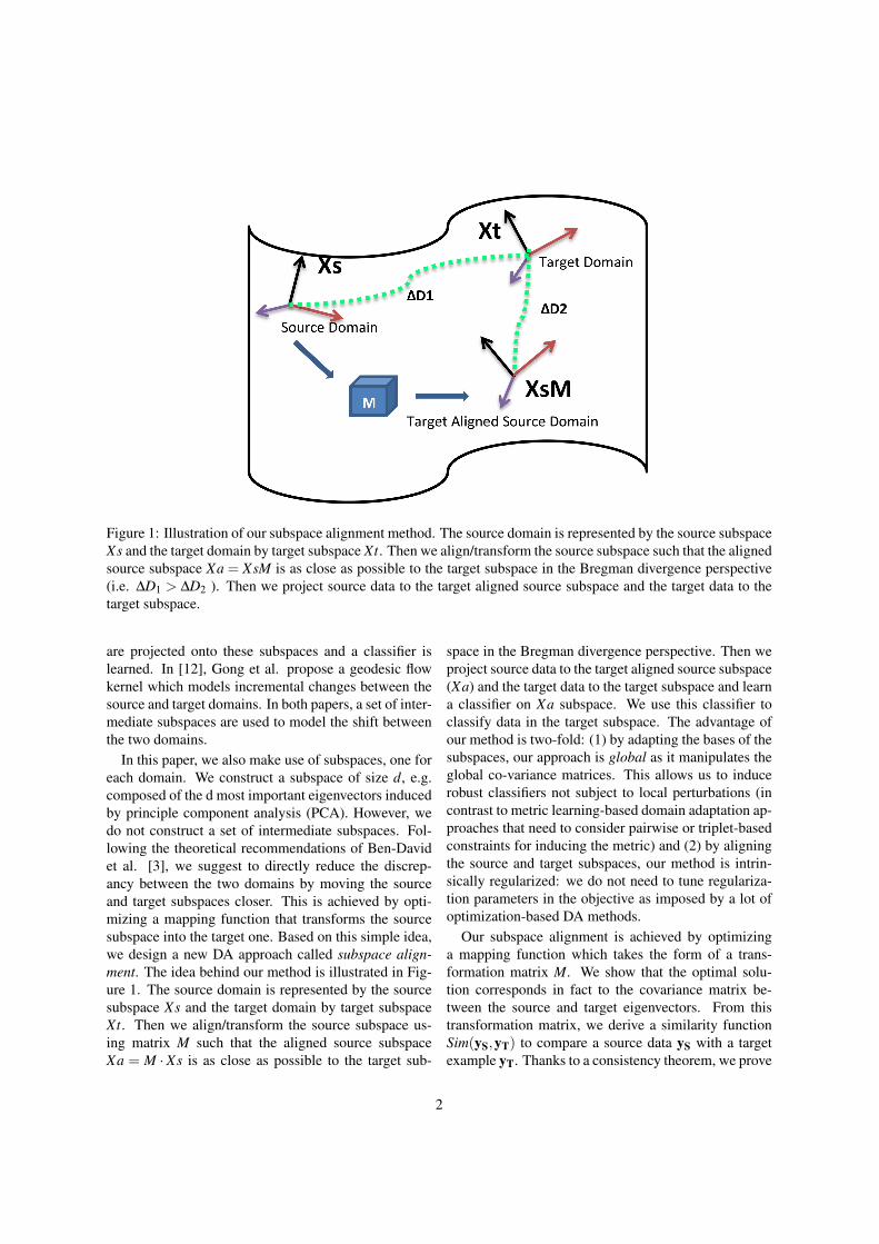
Figure 1: Illustration of our subspace alignment method. The source domain is represented by the source subspaceXs and the target domain by target subspace Xt. Then we align/transform the source subspace such that the alignedsource subspace Xa = XsM is as close as possible to the target subspace in the Bregman divergence perspective(i.e. ∆D1 > ∆D2 ). Then we project source data to the target aligned source subspace and the target data to thetarget subspace.

are projected onto these subspaces and a classifier islearned. In [12], Gong et al. propose a geodesic flowkernel which models incremental changes between thesource and target domains. In both papers, a set of inter-mediate subspaces are used to model the shift betweenthe two domains.

In this paper, we also make use of subspaces, one foreach domain. We construct a subspace of size d, e.g.composed of the d most important eigenvectors inducedby principle component analysis (PCA). However, wedo not construct a set of intermediate subspaces. Fol-lowing the theoretical recommendations of Ben-Davidet al. [3], we suggest to directly reduce the discrep-ancy between the two domains by moving the sourceand target subspaces closer. This is achieved by opti-mizing a mapping function that transforms the sourcesubspace into the target one. Based on this simple idea,we design a new DA approach called subspace align-ment. The idea behind our method is illustrated in Fig-ure 1. The source domain is represented by the sourcesubspace Xs and the target domain by target subspaceXt. Then we align/transform the source subspace us-ing matrix M such that the aligned source subspaceXa = M ·Xs is as close as possible to the target sub-

space in the Bregman divergence perspective. Then weproject source data to the target aligned source subspace(Xa) and the target data to the target subspace and learna classifier on Xa subspace. We use this classifier toclassify data in the target subspace. The advantage ofour method is two-fold: (1) by adapting the bases of thesubspaces, our approach is global as it manipulates theglobal co-variance matrices. This allows us to inducerobust classifiers not subject to local perturbations (incontrast to metric learning-based domain adaptation ap-proaches that need to consider pairwise or triplet-basedconstraints for inducing the metric) and (2) by aligningthe source and target subspaces, our method is intrin-sically regularized: we do not need to tune regulariza-tion parameters in the objective as imposed by a lot ofoptimization-based DA methods.

Our subspace alignment is achieved by optimizinga mapping function which takes the form of a trans-formation matrix M. We show that the optimal solu-tion corresponds in fact to the covariance matrix be-tween the source and target eigenvectors. From thistransformation matrix, we derive a similarity functionSim(yS,yT) to compare a source data yS with a targetexample yT. Thanks to a consistency theorem, we prove

2

that Sim(yS,yT), which captures the idiosyncrasies ofthe training data, converges uniformly to its expectedvalue. We show that we can make use of this theoreticalresult to tune the hyper-parameter d (the dimensional-ity of the subspaces). This tends to make our methodparameter-free. The similarity function Sim(yS,yT) canbe used directly in a nearest neighbour classifier. Al-ternatively, we can also learn a global classifier such asa support vector machine on the source data after map-ping them onto the target aligned source subspace.

As suggested by Ben David et al. [3], a reduction ofthe divergence between the two domains is required toadapt well. In other words, the ability of a DA algo-rithm to actually reduce that discrepancy is a good in-dication of its performance. A usual way to estimatethe divergence consists in learning a linear classifier hto discriminate between source and target instances, re-spectively pseudo-labeled with 0 and 1. In this context,the higher the error of h, the smaller the divergence.While such a strategy gives us some insight about theability for a global learning algorithm (e.g. SVM) tobe efficient on both domains, it does not seem to besuited to deal with local classifiers, such as the k-nearestneighbors. To overcome this limitation, we introduce anew empirical divergence specifically dedicated to localclassifiers. We show through our experimental resultsthat our DA method allows us to drastically reduce bothempirical divergences.

This paper is an extended version of our previouswork [11]. We address a few limitations of the previoussubspace alignment (SA) based DA method. First, thework in [11] does not use source label information dur-ing the subspace creation. Methods such as partial leastsquares (PLS) or linear discriminant analysis (LDA)seem relevant for this task. However, applying differ-ent subspace creation methods such as PLS/LDA onlyfor the source domain and PCA for the target domainmay cause additional discrepancies between the sourceand the target domains. Moreover, LDA has a maxi-mum dimensionality equal to the number of classes. Toovercome these limitations, we use an existing metriclearning algorithm (ITML [9]) to create subspaces in asupervised manner, then use PCA on both the sourceand the target domain. Even though ITML has beenused before for domain adaptation (e.g. [24]), to thebest of our knowledge, it has never been used to cre-ate linear subspaces in conjunction with PCA to im-prove subspace-based domain adaptation methods. Wealso introduce a novel large margin subspace alignment(LMSA) method where the objective is to learn the do-

main adaptive matrix while exploiting the source labelinformation to obtain a discriminative solution. We ex-perimentally show that both these methods are useful inpractice.

Secondly, the cross-validation procedure presented in[11] to estimate the subspace dimensionality could becomputationally expensive for high dimensional data asdiscussed in recent reviews [22]. We propose a fastand well founded approach to estimate the subspace di-mensionality and reduce computational complexity ofour SA method. We call this new extension of SAmethod as SA-MLE. We show promising results usinghigh dimensional data such as Fisher vectors using SA-MLE method. Thirdly, we present a mutual informationbased perspective of our SA method. We show that af-ter the adaptation, with SA method we can increase themutual information between the source and the targetdomains. We also include further analysis and compar-isons in the experimental section. We provide a detailedanalysis of our DA method over several features such asbag-of-words, Fisher vectors [23] and DECAF [10] fea-tures. We also analyze how subspace-based DA meth-ods perform over different dictionary sizes and featurenormalization methods such as z-normalization.

The rest of the paper is organized as follows. Wepresent the related work in section 2. Section 3 isdevoted to the presentation of our domain adaptationmethod and the consistency theorem on the similaritymeasure deduced from the learned mapping function.We also present our supervised PCA method and theSA-MLE method in section 3. In section 4, a compar-ative study is performed on various datasets. We con-clude in section 5.

2 Related workDA has been widely studied in the literature and is ofgreat importance in many areas such as natural lan-guage processing [6] and computer vision [26]. In thispaper, we focus on the unsupervised domain adapta-tion setting that is well suited to vision problems sinceit does not require any labeling information from thetarget domain. This setting makes the problem verychallenging. An important issue is to find out the re-lationship between the two domains. A classical trendis to assume the existence of a domain invariant featurespace and the objective of a large range of DA work isto approximate this space [19].

A classical strategy related to our work consists of

3

learning a new domain-invariant feature representa-tion by looking for a new projection space. PCAbased DA methods have then been naturally investi-gated [8, 20, 21, 1] in order to find a common latentspace where the difference between the marginal dis-tributions of the two domains is minimized with re-spect to the Maximum Mean Discrepancy (MMD) di-vergence. Very recently, Shao et al. [25] have presenteda very similar approach to ours. In this work Shao etal. present a low-rank transfer subspace learning tech-nique that exploits the locality aware reconstruction ina similar way to manifold learning.

Other strategies have been explored as well such asusing metric learning approaches [16, 24] or canonicalcorrelation analysis methods over different views of thedata to find a coupled source-target subspace [5] whereone assumes the existence of a performing linear clas-sifier on the two domains.

In the structural correspondence learning method of[6], Blitzer et al. propose to create a new feature spaceby identifying correspondences among features fromdifferent domains by modeling their correlations withpivot features. Then, they concatenate source and targetdata using this feature representation and apply PCAto find a relevant common projection. In [7], Changtransforms the source data into an intermediate repre-sentation such that each transformed source sample canbe linearly reconstructed by the target samples. Thisis however a local approach. Local methods may failto capture the global distribution information of thesource,target domains. Moreover it is sensitive to noiseand outliers of the source domain that have no corre-spondence in the target one.

Our method is also related to manifold alignmentwhose main objective is to align two datasets fromtwo different manifolds such that they can be projectedto a common subspace [27, 28, 30]. Most of thesemethods [28, 30] need correspondences from the man-ifolds and all of them exploit the local statistical struc-ture of the data unlike our method that captures theglobal distribution structure (i.e. the structure of the co-variances). At the same time methods such as CCA andmanifold alignment methods can the input datasets tobe from different manifolds.

Recently, subspace based DA has demonstrated goodperformance in visual DA [12, 13]. These methodsshare the same principle: first they compute a domainspecific d-dimensional subspace for the source dataand another one for the target data, independently as-sessed by PCA. Then, they project source and target

data into intermediate subspaces (explicitly or implic-itly) along the shortest geodesic path connecting the twod-dimensional subspaces on the Grassmann manifold.They actually model the distribution shift by lookingfor the best intermediate subspaces. These approachesare the closest to ours but, as mentioned in the introduc-tion, it is more appropriate to align the two subspacesdirectly, instead of computing a large number of inter-mediate subspaces which potentially involves a costlytuning procedure. The effectiveness of our idea is sup-ported by our experimental results.

As a summary, our approach has the following differ-ences with existing methods:

We exploit the global co-variance statistical struc-ture of the two domains during the adaptation processin contrast to the manifold alignment methods that uselocal statistical structure of the data [27, 28, 30]. Weproject the source data onto the source subspace and thetarget data onto the target subspace in contrast to meth-ods that project source data to the target subspace or tar-get data to the source subspace such as [5]. Moreover,we do not project data to a large number of subspacesexplicitly or implicitly as in [12, 13]. Our method is un-supervised and does not require any target label infor-mation like constraints on cross-domain data [16, 24] orcorrespondences from across datasets [28, 30]. We donot apply PCA on cross-domain data like in [8, 20, 21]as this can help only if there exist shared features inboth domains. In contrast, we make use of the corre-lated features in both domains. Some of these featurescan be specific to one domain yet correlated to someother shared features in both domains allowing us touse both shared and domain specific features.

3 DA based on unsupervised sub-space alignment

In this section, we introduce our new subspace basedDA method. We assume that we have a set S of labeledsource data (resp. a set T of unlabeled target data) bothlying in a given D-dimensional space and drawn i.i.d.according to a fixed but unknown source distributionP(χS,ϑS) (resp. target distribution P(χT ,ϑT )) whereP(χS,ϑS) 6= P(χT ,ϑT ). We assume that the source la-beling function is more or less similar to the target la-beling function. We denote the transpose operation by′. We denote vectors by lowercase bold fonts such as yiand the class label by notation Li. Matrices are repre-

4

sented by uppercase letters such as X .In section 3.1, we explain how to generate the source

and target subspaces of size d. Then, we present ourDA method in section 3.2 which consists in learninga transformation matrix M that maps the source sub-space to the target one. In section 3.3, we present twomethods to find the subspace dimensionality which isthe only parameter in our method. We present a metriclearning-based source subspace creation method in sec-tion 3.4 which uses labels of source data and our novellarge margin subspace alignment in section 3.5. In sec-tion 3.6 we present a new domain divergence measuresuitable for local classifiers such as the nearest neigh-bour classifier. Finally, in section 3.7 we give a mutualinformation based perspective to our method.

3.1 Subspace generationEven though both the source and target data lie in thesame D-dimensional space, they have been drawn ac-cording to different distributions. Consequently, ratherthan working on the original data themselves, we sug-gest to handle more robust representations of the sourceand target domains and to learn the shift between thesetwo domains. First, we transform every source and tar-get data to a D-dimensional z-normalized vector (i.e.of zero mean and unit standard deviation). Note thatz-normalization is an important step in most of thesubspace-based DA methods such as GFK [12] andGFS [13]. Then, using PCA, we select for each do-main the d eigenvectors corresponding to the d largesteigenvalues. These eigenvectors are used as bases of thesource and target subspaces, respectively denoted by XSand XT (XS,XT ∈ RD×d). Note that X ′S and X ′T are or-thonormal (thus, X ′SXS = Id and X ′T XT = Id where Id isthe identity matrix of size d). In the following, XS andXT are used to learn the shift between the two domains.Sometimes, we refer XS and XT as subspaces, where weactually refer to the basis vectors of the subspace.

3.2 Domain adaptation with subspacealignment

As already presented in section 2, two main strategiesare used in subspace based DA methods. The first oneconsists in projecting both source and target data to acommon shared subspace. However, since this onlyexploits shared features in both domains, it is not al-ways optimal. The second one aims to build a (poten-tially large) set of intermediate representations. Beyond

the fact that such a strategy can be costly, projectingthe data to intermediate common shared subspaces maylead to data explosion.

In our method, we suggest to project each source(yS) and target (yT) data (where yS,yT ∈ R1×D) to itsrespective subspace XS and XT by the operations ySXSand yTXT , respectively. Then, we learn a linear trans-formation that maps the source subspace to the targetone. This step allows us to directly compare sourceand target samples in their respective subspaces with-out unnecessary data projections. To achieve this task,we use a subspace alignment approach. We align basisvectors by using a transformation matrix M from XS toXT (M ∈Rd×d). M is learned by minimizing the follow-ing Bregman matrix divergence:

F(M) = ||XSM−XT ||2F (1)

M∗ = argminM(F(M)) (2)

where ||.||2F is the Frobenius norm. Since XS and XTare generated from the first d eigenvectors, it turns outthat they tend to be intrinsically regularized1. There-fore, we suggest not to add a regularization term in theEq. 1. It is thus possible to obtain a simple solution ofEq. 2 in closed form. Because the Frobenius norm is in-variant to orthonormal operations, we can re-write theobjective function in Eq. 1 as follows:

M∗ = argminM||X ′SXSM−X ′SXT ||2F (3)= argminM||M−X ′SXT ||2F .

From this result, we can conclude that the optimal M∗

is obtained as M∗ = X ′SXT . This implies that the newcoordinate system is equivalent to Xa = XSX ′SXT . Wecall Xa the target aligned source coordinate system. Itis worth noting that if the source and target domains arethe same, then XS = XT and M∗ is the identity matrix.

Matrix M∗ transforms the source subspace coordinatesystem into the target subspace coordinate system byaligning the source basis vectors with the target ones. is

In order to compare a source data yS with a target datayT, one needs a similarity function Sim(yS,yT). Pro-jecting yS and yT in their respective subspace XS and

1We experimented with several regularization methods on thetransformation matrix M such as 2-norm, trace norm, and Frobeniusnorm regularization. None of these regularization strategies improvedover using no regularization.

5

XT and applying the optimal transformation matrix M∗,we can define Sim(yS,yT) as follows:

Sim(yS,yT) = (ySXSM∗)(yTXT )′ = ySXSM∗X ′T yT

′

= ySAyT′, (4)

where A = XSX ′SXT X ′T . Note that Eq. 4 looks likea generalized dot product (even though A is not pos-itive semi-definite) where A encodes the relative con-tributions of the different components of the vectors intheir original space.

We use the matrix A to construct the kernel matri-ces via Sim(yS,yT) and perform SVM-based classifi-cation. To use with nearest neighbour classifier, weproject the source data via Xa into the target alignedsource subspace and the target data into the target sub-space (using XT ), and perform the classification in thisd-dimensional space. The pseudo-code of this algo-rithm is presented in Algorithm 1.

Data: Source data S, Target data T , Source labelsLS, Subspace dimension d

Result: Predicted target labels LTXS← PCA(S,d) ;XT ← PCA(T,d) ;Xa← XSX ′SXT ;Sa = SXa ;TT = T XT ;LT ← NN−Classi f ier(Sa,TT ,LS) ;

Algorithm 1: Subspace alignment DA algorithm inthe lower d-dimensional space

From now on, we will simply use M to refer to M∗.

3.3 Subspace dimensionality estimation

Now we have explained the subspace alignment domainadaptation algorithm in section 3.2, in the following twosubsections we present two methods to find the size ofthe subspace dimensionality which is the unique hyper-parameter of our method. First, in section 3.3.1 wepresent a theoretical result on the stability of the solu-tion and then use this result to tune the subspace dimen-sionality d. In the second method, we use maximumlikelihood estimation to find the intrinsic subspace di-mensionalities of the source domain (ds) and the targetdomain (dt ). Then we use these dimensionalities as be-fore in the SA method. This slightly different version

of SA method is called SA-MLE. SA-MLE does not nec-essarily need to have the same dimensionality for boththe source subspace XS and the target subspace XT . Wepresent SA-MLE method in subsection 3.3.2.

3.3.1 SA: Subspace dimensionality estimation us-ing consistency theorem on Sim(yS,yT)

The unique hyper-parameter of our algorithm is thenumber d of eigenvectors. In this section, inspiredfrom concentration inequalities on eigenvectors [32],we derive an upper bound on the similarity functionSim(yS,yT). Then, we show that we can use this the-oretical result to tune d.

Let Dn be the covariance matrix of a sample D ofsize n drawn i.i.d. from a given distribution and D itsexpected value over that distribution.

Theorem 1. [32] Let B be s.t. for any x,‖x‖ ≤B, let Xd

D and XdDn

be the orthogonal projectors ofthe subspaces spanned by the first d eigenvectors ofD and Dn. Let λ1 > λ2 > ... > λd > λd+1 ≥ 0 bethe first d + 1 eigenvalues of D, then for any n ≥(

4B(λd−λd+1)

(1+√

ln(1/δ )2

))2

with probability at least

1−δ we have:

‖XdD−Xd

Dn‖ ≤ 4B√

n(λd−λd+1)

(1+

√ln(1/δ )

2

).

From this theorem, we can derive the followinglemma for the deviation between Xd

DXdD′ and Xd

DnXd

Dn

′.For the sake of simplification, we will use in the fol-lowing the same notation D (resp. Dn) for defining ei-ther the sample D (resp. Dn) or its covariance matrix D(resp. Dn).

lemma 1. Let B s.t. for any x,‖x‖ ≤ B, let XdD and Xd

Dnthe orthogonal projectors of the subspaces spanned bythe first d eigenvectors of D and Dn. Let λ1 > λ2 >... > λd > λd+1 ≥ 0 be the first d + 1 eigenvalues of

D, then for any n≥(

4B(λd−λd+1)

(1+√

ln(1/δ )2

))2

with

probability at least 1−δ we have:

‖XdDXd

D′−Xd

DnXdDn

′‖≤ 8√

d√n

B(λd−λd+1)

(1+

√ln(1/δ )

2

)

6

Figure 2: Classifying ImageNet images using Caltech-256 images as the source domain. In the first row, we showan ImageNet query image. In the second row, the nearest neighbour image from our method is shown.

Figure 3: Classifying ImageNet images using Caltech-256 images as the source domain. In the first row, we showan ImageNet query image. In the second row, the nearest neighbour image from our method is shown.

Proof.

‖XdDXd

D′−Xd

DnXdDn

′‖

=‖XdDXd

D′−Xd

DXdDn

′+Xd

DXdDn

′−XdDnXd

Dn

′‖

≤‖XdD‖‖Xd

D′−Xd

Dn

′‖+‖XdD−Xd

Dn‖‖XdDn

′‖

≤2√

d√n

4B(λd−λd+1)

(1+

√ln(1/δ )

2

)The last inequality is obtained by the fact that the eigen-vectors are normalized and thus ‖XD‖ ≤

√d and appli-

cation of Theorem 1 twice. We now give a theorem forthe projectors of our DA method.

Theorem 2. Let XdSn

(resp. XdTn

) be the d-dimensionalprojection operator built from the source (resp. target)sample of size nS (resp. nT ) and Xd

S (resp. XdT ) its ex-

pected value with the associated first d +1 eigenvalues

λ S1 > ... > λ S

d > λ Sd+1 (resp. λ T

1 > ... > λ Td > λ T

d+1),then we have with probability at least 1−δ

‖XdS MXd

T′−Xd

SnMnXd

Tn

′‖ ≤ 8d3/2B

(1+

√ln(2/δ )

2

)

×

(1

√nS(λ

Sd −λ S

d+1)+

1√

nT (λ Td −λ T

d+1)

)

where Mn is the solution of the optimization problem ofEq 2 using source and target samples of sizes nS and nTrespectively, and M is its expected value.

7

Proof.

‖XdS MXd

T′−Xd

SnMnXd

Tn

′‖=

‖XdS Xd

S′Xd

T XdT′−Xd

SnXd

Sn

′Xd

TnXd

Tn

′‖

=‖XdS Xd

S′Xd

T XdT′−Xd

S XdS′Xd

TnXd

Tn

′+

XdS Xd

S′Xd

TnXd

Tn

′−XdSn

XdSn

′Xd

TnXd

Tn

′‖

≤‖XdS Xd

S′Xd

T XdT′−Xd

S XdS′Xd

TnXd

Tn

′‖+

‖XdS Xd

S′Xd

TnXd

Tn

′−XdSn

XdSn

′Xd

TnXd

Tn

′‖

≤‖XdS ‖‖X

dS′‖‖Xd

T XdT′−Xd

TnXd

Tn

′‖+

‖XdS Xd

S′−Xd

SnXd

Sn

′‖‖XdTn‖‖Xd

Tn

′‖

≤8d3/2B

(1+

√ln(2/δ )

2

)×(

1√

nS(λSd −λ S

d+1)+

1√

nT (λTd −λ T

d+1)

).

The first equality is obtained by replacing M andMn by their corresponding optimal solutions Xd

S XdT′ and

XdSn

XdTn

′ from Eq 4. The last inequality is obtained byapplying Lemma 1 twice and bounding the projectionoperators.

From Theorem 2, we can deduce a bound on the de-viation between two successive eigenvalues. We canmake use of this bound as a cutting rule for auto-matically determining the size of the subspaces. Letnmin = min(nS,nT ) and (λ min

d − λ mind+1) = min((λ T

d −λ T

d+1),(λSd − λ S

d+1)) and let γ > 0 be a given alloweddeviation such that:

γ ≥

(1+

√ln2/δ

2

)(16d3/2B

√nmin(λ

mind −λ min

d+1)

).

Given a confidence δ > 0 and a fixed deviation γ > 0,we can select the maximum dimension dmax such that:

(λ mindmax−λ

mindmax+1)≥

(1+

√ln2/δ

2

)(16d3/2Bγ√

nmin

).

(5)For each d ∈ d|1 . . .dmax, we then have the guar-

antee that ‖XdS MXd

T′−Xd

SnMnXd

Tn

′‖ ≤ γ . In other words,as long as we select a subspace dimension d such thatd ≤ dmax, the solution M∗ is stable and not prone toover-fitting.

Now we use this theoretical result to obtain the sub-space dimensionality for our method. We have proved a

bound on the deviation between two successive eigen-values. We use it to automatically determine the max-imum size of the subspaces dmax that allows to get astable and non over-fitting matrix M. To find a suitablesubspace dimensionality (d∗ < dmax), we consider allthe subspaces of size d = 1 to dmax and select the best dthat minimizes the classification error using a two foldcross-validation over the labeled source data. Conse-quently, we assume that the source and the target sub-spaces have the same dimensionality. For more detailson the cross-validation procedure see section 4.3.

3.3.2 SA-MLE: Finding the subspace dimensional-ity using maximum likelihood estimation

In this section we present an efficient subspace dimen-sionality estimation method using the maximum likeli-hood estimation to be used in Subspace Alignment forhigh dimensional data when NN classifier is used. Wecall this extension of our SA method SA-MLE. Thereare two problems when applying SA method on high di-mensional data (for example, Fisher vectors [23]). First,the subspace dimensionality estimation using a cross-validation procedure as explained in section 3.3.1 andsection 4.3 could be computationally expensive. Sec-ondly, since we compute the similarity metric in Eq. (4)in the original RD space, the size of the resulting simi-larity metric A is RD×D. For high dimensional data, thisis not efficient.

However, after obtaining the domain transformationmatrix M (using Eq. 1), any classification learningproblem can be formulated in the target aligned sourcesubspace (i.e. XSM) which has smaller dimensional-ity than the original space RD. To reduce the compu-tational effort, we propose to evaluate the sample dis-similarity (DSA−MLE(ys,ys)) between the target alignedsource samples and the target subspace projected targetsamples using Euclidean distance as in Eq. 6 where ysis the source sample and yt is the target sample.

DSA−MLE(ys,yt) = ||ysXSM−ytXT ||2. (6)

The source and target subspaces Xs and Xt are ob-tained by PCA as before. But now the size of the sub-spaces are different: the source subspace is of size dsand the target subspace is of size dt .

dimensionality sourceOne objective of the method described in this section

is to retain the local neighborhood information after di-mensionality reduction. The key reason for selecting

8

this approach is that on average it preserve the localneighborhood information after the dimensionality re-duction. This allows to preserve useful information inrespective domains while adapting the source informa-tion to the target domain. With this purpose, we choosethe domain intrinsic dimensionality obtained throughthe method presented in [17]. Its objective is to derivethe maximum likelihood estimator (MLE) of the dimen-sion d from i.i.d. observations.

MLE estimator assumes that the observations repre-sent an embedding of a lower dimensional sample. Forinstance, we can write y = φ(z) where φ is a contin-uous and sufficiently smooth mapping, and z are sam-pled from a smooth density function f on Rd , with un-known dimensionality d with d < D. In this setting,close neighbors in Rd are mapped to close neighborsin the embedding RD. Let’s fix a point y and assumef (y)≈ const in a small sphere Sy(R) of radius R aroundy. The binomial process N(t,y);0 ≤ t ≤ R whichcounts the observations within distance t from y is

N(t,y) =n

∑i=1

1yi ∈ Sy(t) , (7)

where 1· is the indicator function. By approximating(7) with a Poisson process it can be shown that the max-imum likelihood estimate of the intrinsic dimensional-ity for the data point y is:

d(y) =

[1

N(R,y)

N(R,y)

∑j=1

logR

Θ j(y)

]−1

(8)

where Θ j(y) is the distance from sample y to its jth

nearest neighbor [17].For our experiments we set R to the mean pair-wise

distance among the samples. The intrinsic dimension-ality of a domain is then obtained by the average d =1n ∑

ni=1 d(yi) over all its instances. The two domains

are considered separately, which implies dS 6= dT . ForMLE based dimensionality estimation we use the im-plementation of [18].

3.4 Using the labels of the source domainto improve subspace representation

In this paper we focus on unsupervised domain adap-tation. So far we have created subspaces using PCA,which does not use available label information even

from the source domain. In this section we further in-vestigate whether the available label information fromthe source domain can be exploited to obtain a bet-ter source subspace. One possibility is to use a su-pervised subspace creation (dimensionality reduction)method such as partial least squares (PLS) or linear dis-criminant analysis (LDA). For example [12] uses PLSto exploit the label information in the source domain.

Using PLS or LDA for creating subspaces has twomajor issues. First, the subspaces created by LDA havea dimensionality equal to the number of classes. Thisclearly is a limitation. Moreover, using PLS or LDAonly for the source domain and PCA for the targetdomain causes an additional discrepancy between thesource and the target subspaces (as they are generatedfrom different methods). For example, in the case of SAmethod, it is not clear how to apply consistency theoremon PLS-based subspaces. The subspace disagreementmeasure [12] (SDM) uses principle angles of subspacesto find a good subspace dimensionality. We believe it isnot valid to use PLS for the source domain and PCA forthe target domain when SDM is used as the principleangles generated by PLS and PCA have different mean-ings. To overcome, these issues we propose a simple,yet interesting and effective method to create supervisedsubspaces for subspace-based DA methods.

Our method is motivated by recent metric learning-based cross-domain adaptation method of [24]. Saenkoet al [24], used information theoretic metric learn-ing method [9] (ITML) to construct cross-domain con-straints to obtain a distance metric in semi-superviseddomain adaptation. They use labelled samples fromboth the source and the target domains to construct adistance metric that can be used to compare a sourcesample with target domain samples. We also use theinformation theoretic metric learning (ITML) method[9] to create a distance metric only for the source do-main using the labeled source samples. In contrast tothe work of Saenko et al. [24], we use this learnedmetric to transform source data into the metric inducedspace such that the discriminative nature of the sourcedata is preserved. Afterwards, we apply PCA on thetransformed source data samples to obtain the eigenvec-tors for our subspace alignment method. The proposednew algorithm to create supervised source subspace isshown in Algo. 2.

The advantage of our method is that the source andtarget subspaces are still created using the same PCAalgorithm as before. As a result we can still use theconsistency theorem to find a stable subspace dimen-

9

sionality. In addition, we show that not only it improvesresults for our SA method, but also for other subspacebased methods such as GFK.

Data: Source data S, Source labels LSResult: Source subspace Xs1. Learn the source metric W ← IT ML(S,LS) ;2. Apply cholesky-decomposition to W .Wc← chol(W ) ;3. Project source data to Wc induced space.Sw← SWc ;4. Xs← PCA(Sw) ;

Algorithm 2: Source Subspace learning algorithmwith metric learning - (ITML-PCA method)

3.5 LMSA: Large-Margin SubspaceAlignment

Motivated by the above approach, we propose a morefounded optimization strategy to incorporate the classinformation from the source domain during DA learn-ing procedure. To preserve discriminative informationin the source domain, we try to minimize pairwise dis-tances between samples from the same class. At thesame time utilizing triplets, we make sure that samplesfrom different classes are well separated by a large mar-gin. To achieve this motivation we modify the objectivefunction in Eq. 1 as follows:

F(M) = ||XSM−XT ||2F +β1 ∑(i, j)∈Ω

di, j+

β2 ∑i, j,k

max(0,1− (di,k−di, j)) (9)

where Ω = i, j is the set of all source image pairsfrom the same class. The triplet i, j,k are createdsuch that i, j are from the same class and j ∈ 3NN(i)while i,k are from different classes (i, j,k are fromthe source domain). We generate all possible suchtriplets. The parameters β1,β2 > 0. The Euclidean dis-tance (di, j) between pair of images projected into targetaligned source subspace is defined as follows:

di, j = ||ySiXSM−ySj XSM||2. (10)

We call this approach as LMSA.

3.6 Divergence between source and targetdomains

If one can estimate the differences between domains,then this information can be used to estimate the diffi-culty of adapting the source domain to a specific targetdomain. Further, such domain divergence measures canbe used to evaluate the effectiveness of domain adap-tation methods. In this section we discuss two domaindivergence measures, one suitable for global classifierssuch as support vector machines and the other useful forlocal classifiers such as nearest neighbour classifiers.Note we consider, nearest neighbour as a local classi-fier as the final label of the test sample only dependson the local neighborhood distribution of the trainingdata. At the same time we consider a SVM classifieras a global classifier as SVM possibly depends on alltraining samples.

Ben-David et al. [3] provide a generalization boundon the target error which depends on the source er-ror and a measure of divergence, called the H∆H di-vergence, between the source and target distributionsP(χS) and P(χT ).

εT (h) = εS(h)+dH∆H(P(χS),P(χT ))+λ , (11)

where h is a learned hypothesis, εT (h) the generaliza-tion target error, εS(h) the generalization source error,and λ the error of the ideal joint hypothesis on S and T ,which is supposed to be a negligible term if the adapta-tion is possible. Eq. 11 tells us that to adapt well, onehas to learn a hypothesis which works well on S whilereducing the divergence between P(χS) and P(χT ). Toestimate dH∆H(P(χS),P(χT )), a usual way consists inlearning a linear classifier h to discriminate betweensource and target instances, respectively pseudo-labeledwith 0 and 1. In this context, the higher the error of h,the smaller the divergence. While such a strategy givesus some insight about the ability for a global learningalgorithm (e.g. SVM) to be efficient on both domains, itdoes not seem to be suited to deal with local classifiers,such as k-nearest neighbors. To overcome this limita-tion, we introduce a new empirical divergence specifi-cally designed for local classifiers. Based on the recom-mendations of [4], we propose a discrepancy measure toestimate the local density of a target point w.r.t. a givensource point. This discrepancy, called Target densityaround source TDAS counts on average how many tar-get points can be found within a ε neighborhood of asource point. More formally:

10

T DAS =1nS

∑∀yS

|yT|Sim(yS,yT)≥ ε|. (12)

Note that TDAS is associated with similarity mea-sure Sim(yS,yT) = ySAyT

′ where A is the learned met-ric. As we will see in the next section, TDAS can beused to evaluate the effectiveness of a DA method un-der the covariate shift assumption and probabilistic Lip-schitzness assumption [4]. The larger the TDAS, thebetter the DA method.

3.7 Mutual information perspective onsubspace alignment

Finally, in this section we look at subspace alignmentfrom a mutual information point of view. We start thisdiscussion with a slight abuse of notations. We denoteH(S) as the entropy of the source data S and H(S,T )the cross entropy between the source data S and the tar-get data T . The mutual information between the sourcedomain S and the target domain T then can be given asfollows:

MI(S;T ) = H(S)+H(T )−H(S,T )

= H(T )−DKL(S||T ).(13)

According to Eq. (13), if we maximize the target en-tropy (i.e. H(T )) and minimize the KL-divergence (i.e.DKL(S||T ) term), we maximize the mutual informationMI(S;T ). In domain adaptation it makes sense to max-imize the mutual information between the source do-main and the target domain. If one projects data fromall domains to the target subspace XT , then this allowsto increase the entropy term H(T ), hence the mutualinformation MI(S;T ). This could be a reason why pro-jecting to the target subspace performs quite well forsome DA problems as reported by our previous work[11] and other related work [12]. We also project thetarget data to the target subspace which allows to maxi-mize the term H(T ).

For the simplicity of derivation, we assume thesource and the target data are drawn from a zero cen-tered Gaussian distribution. Then the KL-divergencebetween the source domain and the target domain canbe written as follows:

DKL(S||T ) =12(tr(Σ−1

t Σs)−d− ln(det(Σs)

det(Σt))) (14)

where Σ is the covariance matrix, tr() is the trace ofa matrix and det() is the determinant of the matrix. Theterm Σ

−1t Σs can be written as follows:

Σ−1t Σs = XsΛsX ′sXtΛ

−1t X ′t (15)

where Λ is a diagonal matrix constituted of eigenval-ues λ .

The term in Eq. 15 is minimized if basis vectors of Xsare aligned with the basis vectors in Xt . In SA method,by aligning the two subspaces we indirectly minimizethe tr(Σ−1

t Σs) term. Aligning all basis vectors doesnot contribute equally as the basis vectors with highereigenvalues (λs,λt ) are the most influential. So we haveto align the most important d number of basis vectors.This step allows us to reduce the KL-divergence be-tween the source and the target domain. In summary,the subspace alignment method optimizes both criteriagiven in equation 13, which allows us to maximize themutual information between the source distribution andthe target distribution.

4 ExperimentsWe evaluate our domain adaptation approach in the con-text of object recognition using a standard dataset andprotocol for evaluating visual domain adaptation meth-ods as in [7, 12, 13, 16, 24]. In addition, we also evalu-ate our method using various other image classificationdatasets. We denote our subspace alignment method bySA and the maximum likelihood estimation based SAmethods as SA-MLE. Unless specifically mentioned, bydefault we consider SA method in rest of the experi-ments.

First, in section 4.1 we present the datasets. Then insection 4.2 we present the experimental setup. Exper-imental details about subspace dimensionality estima-tion for the consistency theorem-based SA method arepresented in section 4.3. Then we evaluate consideredsubspace-based methods using two domain divergencemeasures in section 4.4. In section 4.5 we evaluate theclassification performance of the proposed DA methodusing three DA-based object recognition datasets. Thenin section 4.6 we present the effectiveness of super-vised subspace creation-based SA method. We analyzethe performance of subspace-based DA methods whenused with high dimensional data such as Fisher vectorsin section 4.7. In section 4.8 we analyze the perfor-mance of DA methods by varying the dictionary size of

11

the bag-of-words. We evaluate the effectiveness of sub-space based DA methods using modern deep learningfeatures in section 4.9. The influence of z-normalizationon DA methods is analyzed in section 4.10. Finally,we compare our SA method with non-subspace-basedmethods in section 4.11.

4.1 DA datasets and data preparation

We provide three series of classification experimentson different datasets. In the first series, we use theOffice+Caltech-10 [12] dataset that contains four do-mains altogether to evaluate all DA methods (see Fig-ure 4). The Office dataset [24] consists of images fromweb-cam (denoted by W), DSLR images (denoted byD) and Amazon images (denoted by A). The Caltech-10images are denoted by C. We follow the same setup asin [12]. We use each source of images as a domain, con-sequently we get four domains (A, C, D and W) leadingto 12 DA problems. We denote a DA problem by thenotation S→ T . We use the image representations pro-vided by [12] for Office and Caltech10 datasets (SURFfeatures encoded with a visual dictionary of 800 words).We follow the standard protocol of [12, 13, 16, 24] forgenerating the source and target samples.

In a second series, we evaluate the effectiveness ofour DA method using other datasets, namely ImageNet(I), LabelMe (L) and Caltech-256 (C). In this setting weconsider each dataset as a domain. We select five objectcategories common to all three datasets (bird, car, chair,dog and person) leading to a total of 7719 images. Weextract dense SIFT features and create a bag-of-wordsdictionary of 256 words using kmeans. Afterwards, weuse LLC encoding and a spatial pyramid (2× 2 quad-rants + 3×1 horizontal + 1 full image) to obtain a 2048dimensional image representation (similar data prepa-ration as in [14]).

In the last series, we evaluate the effectiveness ofour DA method using larger datasets, namely PASCAL-VOC-2007 and ImageNet. We select all the classes ofPASCAL-VOC-2007. The objective here is to classifyPASCAL-VOC-2007 test images using classifiers thatare learned from the ImageNet dataset. To prepare thedata, we extract dense SIFT features and create a bag-of-words dictionary of 256 words using only ImageNetimages. Afterwards, we use LLC encoding and spatialpyramids (2× 2 + 3× 1 + 1) to obtain a 2048 dimen-sional image representation.

4.2 Experimental setup

We compare our subspace DA approach with threeother DA methods and three baselines. Each of thesemethods defines a new representation space and ourgoal is to compare the performance of a 1-Nearest-Neighbor (NN) classifier and a linear SVM classifieron DA problems in the subspace found.

We naturally consider Geodesic Flow Kernel (GFK[12]), Geodesic Flow Sampling (GFS [13]) and Trans-fer Component Analysis (TCA) [21]. They have indeeddemonstrated state of the art performances achievingbetter results than metric learning methods [24] and bet-ter than those reported by Chang’s method in [7]. More-over, these methods are conceptually the closest to ourapproach. We also report results obtained by the fol-lowing three baselines:

• Baseline-S: where we use the projection defined bythe PCA subspace XS built from the source domainto project both source and target data and work in theresulting representation.

• Baseline-T: where we use similarly the projectiondefined by the PCA subspace XT built from the targetdomain.

• No adaptation NA: where no projection is made, i.e.we use the original input space without learning anew representation.

For each method, we compare the performance ofa 1-Nearest-Neighbor (NN) classifier and of a linearSVM classifier (we seek the best C parameter aroundthe mean similarity value obtained from the trainingset) in the subspace defined by each method. For eachsource-target DA problem in the first two series of ex-periments, we evaluate the accuracy of each methodon the target domain over 20 random trials. For eachtrial, we consider an unsupervised DA setting where werandomly sample labeled data in the source domain astraining data and unlabeled data in the target domain astesting examples. For the first series we use the typicalsetup as in [12]. For the second series we use a max-imum of 100 randomly sampled training images per-class. In the last series involving the PASCAL-VOCdataset, we evaluate the approaches by measuring themean average precision over target data using SVM.

12

Figure 4: Some example images from Office-Caltech dataset. This dataset consists of four visual domains, namelyimages collected from Amazon merchant website, images collected from a high resolution DSLR camera, imagescollected from a web camera and images collected from Caltech-101 dataset.

4.3 Selecting the optimal dimensionalityfor the SA method using the consis-tency theorem

In this section, we present the procedure for select-ing the space dimensionality in the context of the SAmethod. The same dimensionality is also used forBaseline-S and Baseline-T. For GFK and GFS we fol-low the published procedures to obtain optimal resultsas presented in [12]. First, we perform a PCA on thetwo domains and compute the deviation λ min

d − λ mind+1

for all possible d values. Then, using the theoreticalbound of Eq: 5, we can estimate a dmax << D that pro-vides a stable solution with fixed deviation γ > 0 for agiven confidence δ > 0. Afterwards, we consider thesubspaces of dimensionality from d = 1 to dmax and se-lect the best d∗ that minimizes the classification errorusing a 2 fold cross-validation over the labelled sourcedata. This procedure is founded by the theoretical re-sult of Ben-David et al. of Eq 11 where the idea is totry to move closer the domain distribution while main-taining a good accuracy on the source domain. As anillustration, the best dimensions for the Office+Caltechdataset varies between 10− 50. For example, for theDA problem W→ C, taking γ = 105 and δ = 0.1, weobtain dmax = 22 (see Figure 5) and by cross validationwe found that the optimal dimension is d∗ = 20.

4.4 Evaluating DA with divergence mea-sures

Here, we evaluate the capability of our SA method tomove closer the domain distributions according to themeasures presented in Section 3.6: the TDAS adapted

Figure 5: Finding a stable solution and a subspace di-mensionality using the consistency theorem. We plotthe bounds for W →C DA problem taking γ = 105 andδ = 0.1. The upper bound is plotted in red color andthe difference in consecutive eigenvalues in black color.From this plot we select the dmax = 22 .

to NN classification where a high value indicates a bet-ter distribution closeness and the H∆H using a SVMwhere a value close to 50 indicates close distributions.

To compute H∆H using a SVM we use the follow-ing protocol. For each baseline method, SA and GFKwe apply DA using both source and target data. Af-terwards, we give label +1 for the source samples andlabel −1 for the target samples. Then we randomly di-vide the source samples into two sets of equal size. Thesource train set (Strain) and source test set (Stest ). Werepeat this for the target samples and obtain target trainset (Ttrain) and target test set (Ttest ). Finally, we traina linear SVM classifier using (Strain) and (Ttrain) as thetraining data and evaluate on the test set consisting of(Stest ) and (Ttest ). The final classification rate obtained

13

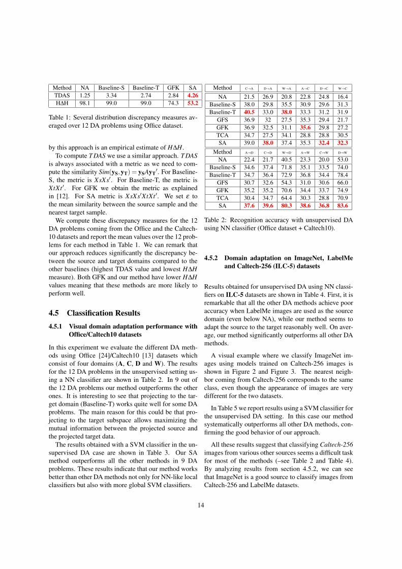
Method NA Baseline-S Baseline-T GFK SATDAS 1.25 3.34 2.74 2.84 4.26H∆H 98.1 99.0 99.0 74.3 53.2

Table 1: Several distribution discrepancy measures av-eraged over 12 DA problems using Office dataset.

by this approach is an empirical estimate of H∆H.To compute T DAS we use a similar approach. T DAS

is always associated with a metric as we need to com-pute the similarity Sim(yS,yT) = ySAyT

′. For Baseline-S, the metric is XsXs′. For Baseline-T, the metric isXtXt ′. For GFK we obtain the metric as explainedin [12]. For SA metric is XsXs′XtXt ′. We set ε tothe mean similarity between the source sample and thenearest target sample.

We compute these discrepancy measures for the 12DA problems coming from the Office and the Caltech-10 datasets and report the mean values over the 12 prob-lems for each method in Table 1. We can remark thatour approach reduces significantly the discrepancy be-tween the source and target domains compared to theother baselines (highest TDAS value and lowest H∆Hmeasure). Both GFK and our method have lower H∆Hvalues meaning that these methods are more likely toperform well.

4.5 Classification Results4.5.1 Visual domain adaptation performance with

Office/Caltech10 datasets

In this experiment we evaluate the different DA meth-ods using Office [24]/Caltech10 [13] datasets whichconsist of four domains (A, C, D and W). The resultsfor the 12 DA problems in the unsupervised setting us-ing a NN classifier are shown in Table 2. In 9 out ofthe 12 DA problems our method outperforms the otherones. It is interesting to see that projecting to the tar-get domain (Baseline-T) works quite well for some DAproblems. The main reason for this could be that pro-jecting to the target subspace allows maximizing themutual information between the projected source andthe projected target data.

The results obtained with a SVM classifier in the un-supervised DA case are shown in Table 3. Our SAmethod outperforms all the other methods in 9 DAproblems. These results indicate that our method worksbetter than other DA methods not only for NN-like localclassifiers but also with more global SVM classifiers.

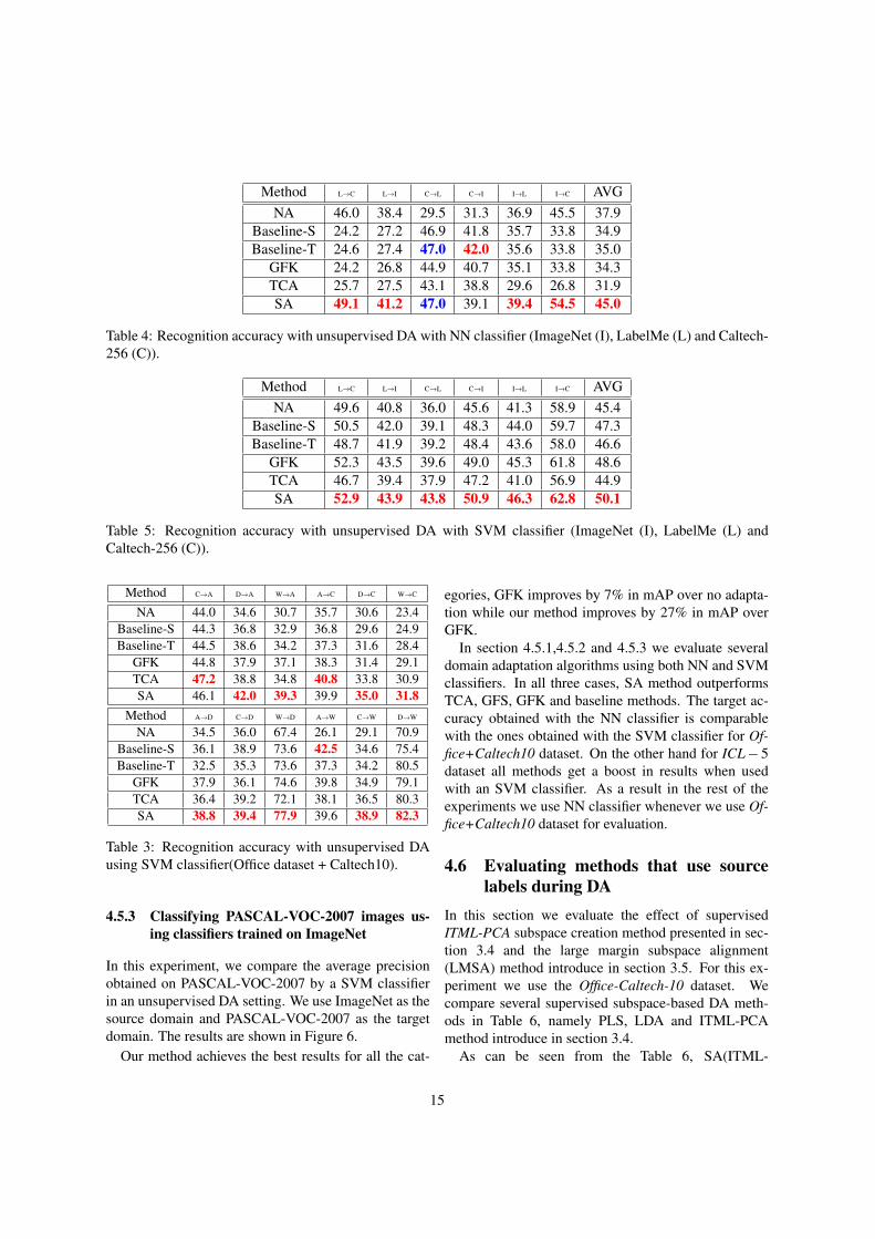
Method C→A D→A W→A A→C D→C W→C

NA 21.5 26.9 20.8 22.8 24.8 16.4Baseline-S 38.0 29.8 35.5 30.9 29.6 31.3Baseline-T 40.5 33.0 38.0 33.3 31.2 31.9

GFS 36.9 32 27.5 35.3 29.4 21.7GFK 36.9 32.5 31.1 35.6 29.8 27.2TCA 34.7 27.5 34.1 28.8 28.8 30.5SA 39.0 38.0 37.4 35.3 32.4 32.3

Method A→D C→D W→D A→W C→W D→W

NA 22.4 21.7 40.5 23.3 20.0 53.0Baseline-S 34.6 37.4 71.8 35.1 33.5 74.0Baseline-T 34.7 36.4 72.9 36.8 34.4 78.4

GFS 30.7 32.6 54.3 31.0 30.6 66.0GFK 35.2 35.2 70.6 34.4 33.7 74.9TCA 30.4 34.7 64.4 30.3 28.8 70.9SA 37.6 39.6 80.3 38.6 36.8 83.6

Table 2: Recognition accuracy with unsupervised DAusing NN classifier (Office dataset + Caltech10).

4.5.2 Domain adaptation on ImageNet, LabelMeand Caltech-256 (ILC-5) datasets

Results obtained for unsupervised DA using NN classi-fiers on ILC-5 datasets are shown in Table 4. First, it isremarkable that all the other DA methods achieve pooraccuracy when LabelMe images are used as the sourcedomain (even below NA), while our method seems toadapt the source to the target reasonably well. On aver-age, our method significantly outperforms all other DAmethods.

A visual example where we classify ImageNet im-ages using models trained on Caltech-256 images isshown in Figure 2 and Figure 3. The nearest neigh-bor coming from Caltech-256 corresponds to the sameclass, even though the appearance of images are verydifferent for the two datasets.

In Table 5 we report results using a SVM classifier forthe unsupervised DA setting. In this case our methodsystematically outperforms all other DA methods, con-firming the good behavior of our approach.

All these results suggest that classifying Caltech-256images from various other sources seems a difficult taskfor most of the methods (–see Table 2 and Table 4).By analyzing results from section 4.5.2, we can seethat ImageNet is a good source to classify images fromCaltech-256 and LabelMe datasets.

14

Method L→C L→I C→L C→I I→L I→C AVGNA 46.0 38.4 29.5 31.3 36.9 45.5 37.9

Baseline-S 24.2 27.2 46.9 41.8 35.7 33.8 34.9Baseline-T 24.6 27.4 47.0 42.0 35.6 33.8 35.0

GFK 24.2 26.8 44.9 40.7 35.1 33.8 34.3TCA 25.7 27.5 43.1 38.8 29.6 26.8 31.9SA 49.1 41.2 47.0 39.1 39.4 54.5 45.0

Table 4: Recognition accuracy with unsupervised DA with NN classifier (ImageNet (I), LabelMe (L) and Caltech-256 (C)).

Method L→C L→I C→L C→I I→L I→C AVGNA 49.6 40.8 36.0 45.6 41.3 58.9 45.4

Baseline-S 50.5 42.0 39.1 48.3 44.0 59.7 47.3Baseline-T 48.7 41.9 39.2 48.4 43.6 58.0 46.6

GFK 52.3 43.5 39.6 49.0 45.3 61.8 48.6TCA 46.7 39.4 37.9 47.2 41.0 56.9 44.9SA 52.9 43.9 43.8 50.9 46.3 62.8 50.1

Table 5: Recognition accuracy with unsupervised DA with SVM classifier (ImageNet (I), LabelMe (L) andCaltech-256 (C)).

Method C→A D→A W→A A→C D→C W→C

NA 44.0 34.6 30.7 35.7 30.6 23.4Baseline-S 44.3 36.8 32.9 36.8 29.6 24.9Baseline-T 44.5 38.6 34.2 37.3 31.6 28.4

GFK 44.8 37.9 37.1 38.3 31.4 29.1TCA 47.2 38.8 34.8 40.8 33.8 30.9SA 46.1 42.0 39.3 39.9 35.0 31.8

Method A→D C→D W→D A→W C→W D→W

NA 34.5 36.0 67.4 26.1 29.1 70.9Baseline-S 36.1 38.9 73.6 42.5 34.6 75.4Baseline-T 32.5 35.3 73.6 37.3 34.2 80.5

GFK 37.9 36.1 74.6 39.8 34.9 79.1TCA 36.4 39.2 72.1 38.1 36.5 80.3SA 38.8 39.4 77.9 39.6 38.9 82.3

Table 3: Recognition accuracy with unsupervised DAusing SVM classifier(Office dataset + Caltech10).

4.5.3 Classifying PASCAL-VOC-2007 images us-ing classifiers trained on ImageNet

In this experiment, we compare the average precisionobtained on PASCAL-VOC-2007 by a SVM classifierin an unsupervised DA setting. We use ImageNet as thesource domain and PASCAL-VOC-2007 as the targetdomain. The results are shown in Figure 6.

Our method achieves the best results for all the cat-

egories, GFK improves by 7% in mAP over no adapta-tion while our method improves by 27% in mAP overGFK.

In section 4.5.1,4.5.2 and 4.5.3 we evaluate severaldomain adaptation algorithms using both NN and SVMclassifiers. In all three cases, SA method outperformsTCA, GFS, GFK and baseline methods. The target ac-curacy obtained with the NN classifier is comparablewith the ones obtained with the SVM classifier for Of-fice+Caltech10 dataset. On the other hand for ICL− 5dataset all methods get a boost in results when usedwith an SVM classifier. As a result in the rest of theexperiments we use NN classifier whenever we use Of-fice+Caltech10 dataset for evaluation.

4.6 Evaluating methods that use sourcelabels during DA

In this section we evaluate the effect of supervisedITML-PCA subspace creation method presented in sec-tion 3.4 and the large margin subspace alignment(LMSA) method introduce in section 3.5. For this ex-periment we use the Office-Caltech-10 dataset. Wecompare several supervised subspace-based DA meth-ods in Table 6, namely PLS, LDA and ITML-PCAmethod introduce in section 3.4.

As can be seen from the Table 6, SA(ITML-

15

Figure 6: Train on ImageNet and classify PASCAL-VOC-2007 images using unsupervised DA with a linear SVMclassifier. Average average precision over 20 object classes is reported.

PCA,PCA) performs better than SA(LDA,PCA) andSA(PLS,PCA).SA(LDA,PCA) reports on average a mean accuracyof 43.0% over 12 DA problems while the SA(ITML-PCA,PCA) method reports the best mean accuracy of48.5 %. ITML-PCA method also improves GFK resultsby 1.2% showing the general applicability of this ap-proach. GFK(PLS,PCA) and GFK(LDA,PLS) report amean accuracy of 42.5% while GFK(ITML-PCA,PCA)reports an accuracy of 43.7 %. This clearly shows thatthe (ITML-PCA) strategy obtains better results for GFKas well as for the SA method. SA(PLS,PCA) reports avery poor accuracy of 38.7%. This could be due to thefact that when PLS is used, the upper bound obtained byconsistency theorem does not hold anymore and we arelikely to obtain a subspace dimension that only works inthe source domain. In contrast, the ITML-PCA methodstill uses PCA to create a linear subspace and so theconsistency theorem holds.

ITML uses both similarity and dissimilarity con-straints using an information theoretic procedure. Thelearned metric W in Algorithm (2) is regularized bylogdet regularization during the ITML procedure. Themetric learning objective makes the subspace discrim-inative while allowing the domain transfer using SAmethod. From this result we conclude that SA(IT ML−PCA,PCA) is a better approach for subspace alignment-based domain adaptation as well as GFK method. In fu-ture work we plan to incorporate ITML [9] like objec-tive directly in the subspace alignment objective func-tion similar to LMSA method.

4.7 Evaluating SA-MLE method usinghigh dimensional data

Despite having a large dimensionality, Fisher vectors[23] have proven to be a robust image representationfor image classification task. One limitation of sub-space alignment is the computational complexity asso-ciated with high dimensional data (see section 3.3.2).We overcome this issue using SA-MLE method.

In this experiment we also use the Office dataset [24]as well as the Office+Caltech-10 dataset. The reasonis that the Office dataset consists of more object classesand images (even though it has only three domains). Weextract SURF [2] features to create a Gaussian mixturemodel (GMM) of 64 components and encode imagesusing Fisher encoding [23]. The GMM is created fromAmazon images from the Office dataset.

Results on the Office dataset using Fisher vectorsare shown in Table 7 while in Table 8 results forOffice+Caltech-10 is reported. These results indicatethe effectiveness of SA-MLE method considering thefact that it can estimate the subspace dimensionality al-most 100 times faster than SA method when used withFisher vectors. On average, SA-MLE outperforms noadaptation (NA) results. Since MLE method returnstwo different subspace dimensionality for the sourceand the target, it is not clear how we can apply MLEmethod on GFK.

Note that SA-MLE is fast and operates in the low-dimensional target subspace. More importantly SA-MLE seems to work well with Fisher vectors. Thecomputational complexity of SA-MLE equal to O(d2)where d is the target subspace dimensionality. On the

16

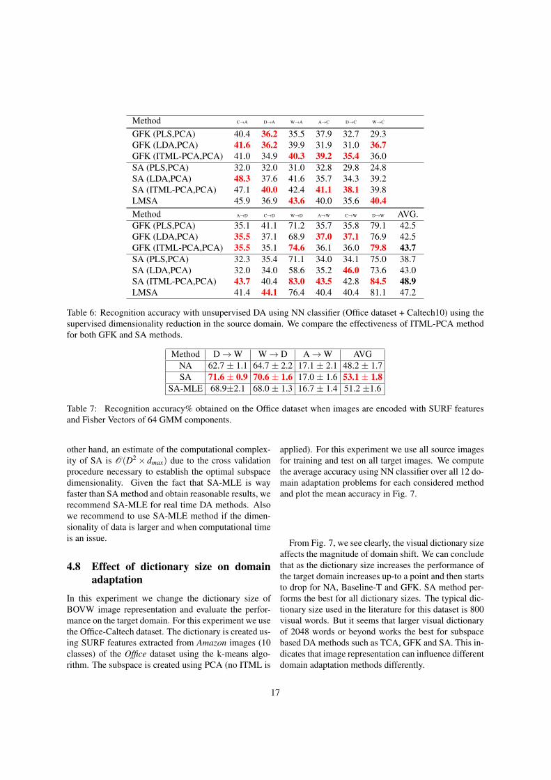
Method C→A D→A W→A A→C D→C W→C

GFK (PLS,PCA) 40.4 36.2 35.5 37.9 32.7 29.3GFK (LDA,PCA) 41.6 36.2 39.9 31.9 31.0 36.7GFK (ITML-PCA,PCA) 41.0 34.9 40.3 39.2 35.4 36.0SA (PLS,PCA) 32.0 32.0 31.0 32.8 29.8 24.8SA (LDA,PCA) 48.3 37.6 41.6 35.7 34.3 39.2SA (ITML-PCA,PCA) 47.1 40.0 42.4 41.1 38.1 39.8LMSA 45.9 36.9 43.6 40.0 35.6 40.4Method A→D C→D W→D A→W C→W D→W AVG.GFK (PLS,PCA) 35.1 41.1 71.2 35.7 35.8 79.1 42.5GFK (LDA,PCA) 35.5 37.1 68.9 37.0 37.1 76.9 42.5GFK (ITML-PCA,PCA) 35.5 35.1 74.6 36.1 36.0 79.8 43.7SA (PLS,PCA) 32.3 35.4 71.1 34.0 34.1 75.0 38.7SA (LDA,PCA) 32.0 34.0 58.6 35.2 46.0 73.6 43.0SA (ITML-PCA,PCA) 43.7 40.4 83.0 43.5 42.8 84.5 48.9LMSA 41.4 44.1 76.4 40.4 40.4 81.1 47.2

Table 6: Recognition accuracy with unsupervised DA using NN classifier (Office dataset + Caltech10) using thesupervised dimensionality reduction in the source domain. We compare the effectiveness of ITML-PCA methodfor both GFK and SA methods.

Method D→W W→ D A→W AVGNA 62.7 ± 1.1 64.7 ± 2.2 17.1 ± 2.1 48.2 ± 1.7SA 71.6 ± 0.9 70.6 ± 1.6 17.0 ± 1.6 53.1 ± 1.8

SA-MLE 68.9±2.1 68.0 ± 1.3 16.7 ± 1.4 51.2 ±1.6

Table 7: Recognition accuracy% obtained on the Office dataset when images are encoded with SURF featuresand Fisher Vectors of 64 GMM components.

other hand, an estimate of the computational complex-ity of SA is O(D2× dmax) due to the cross validationprocedure necessary to establish the optimal subspacedimensionality. Given the fact that SA-MLE is wayfaster than SA method and obtain reasonable results, werecommend SA-MLE for real time DA methods. Alsowe recommend to use SA-MLE method if the dimen-sionality of data is larger and when computational timeis an issue.

4.8 Effect of dictionary size on domainadaptation

In this experiment we change the dictionary size ofBOVW image representation and evaluate the perfor-mance on the target domain. For this experiment we usethe Office-Caltech dataset. The dictionary is created us-ing SURF features extracted from Amazon images (10classes) of the Office dataset using the k-means algo-rithm. The subspace is created using PCA (no ITML is

applied). For this experiment we use all source imagesfor training and test on all target images. We computethe average accuracy using NN classifier over all 12 do-main adaptation problems for each considered methodand plot the mean accuracy in Fig. 7.

From Fig. 7, we see clearly, the visual dictionary sizeaffects the magnitude of domain shift. We can concludethat as the dictionary size increases the performance ofthe target domain increases up-to a point and then startsto drop for NA, Baseline-T and GFK. SA method per-forms the best for all dictionary sizes. The typical dic-tionary size used in the literature for this dataset is 800visual words. But it seems that larger visual dictionaryof 2048 words or beyond works the best for subspacebased DA methods such as TCA, GFK and SA. This in-dicates that image representation can influence differentdomain adaptation methods differently.

17

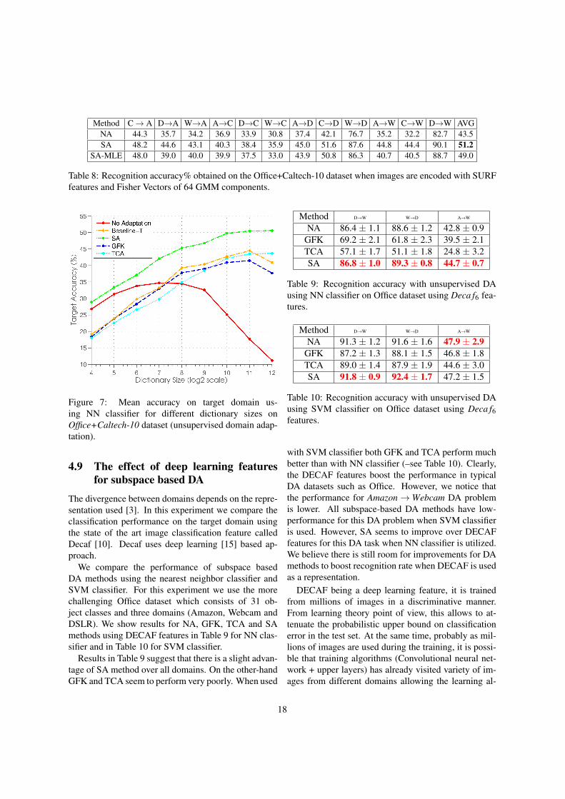
Method C→ A D→A W→A A→C D→C W→C A→D C→D W→D A→W C→W D→W AVGNA 44.3 35.7 34.2 36.9 33.9 30.8 37.4 42.1 76.7 35.2 32.2 82.7 43.5SA 48.2 44.6 43.1 40.3 38.4 35.9 45.0 51.6 87.6 44.8 44.4 90.1 51.2

SA-MLE 48.0 39.0 40.0 39.9 37.5 33.0 43.9 50.8 86.3 40.7 40.5 88.7 49.0

Table 8: Recognition accuracy% obtained on the Office+Caltech-10 dataset when images are encoded with SURFfeatures and Fisher Vectors of 64 GMM components.

Figure 7: Mean accuracy on target domain us-ing NN classifier for different dictionary sizes onOffice+Caltech-10 dataset (unsupervised domain adap-tation).

4.9 The effect of deep learning featuresfor subspace based DA

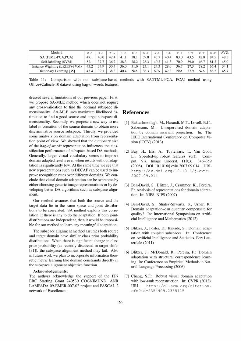
The divergence between domains depends on the repre-sentation used [3]. In this experiment we compare theclassification performance on the target domain usingthe state of the art image classification feature calledDecaf [10]. Decaf uses deep learning [15] based ap-proach.

We compare the performance of subspace basedDA methods using the nearest neighbor classifier andSVM classifier. For this experiment we use the morechallenging Office dataset which consists of 31 ob-ject classes and three domains (Amazon, Webcam andDSLR). We show results for NA, GFK, TCA and SAmethods using DECAF features in Table 9 for NN clas-sifier and in Table 10 for SVM classifier.

Results in Table 9 suggest that there is a slight advan-tage of SA method over all domains. On the other-handGFK and TCA seem to perform very poorly. When used

Method D→W W→D A→W

NA 86.4 ± 1.1 88.6 ± 1.2 42.8 ± 0.9GFK 69.2 ± 2.1 61.8 ± 2.3 39.5 ± 2.1TCA 57.1 ± 1.7 51.1 ± 1.8 24.8 ± 3.2SA 86.8 ± 1.0 89.3 ± 0.8 44.7 ± 0.7

Table 9: Recognition accuracy with unsupervised DAusing NN classifier on Office dataset using Deca f6 fea-tures.

Method D→W W→D A→W

NA 91.3 ± 1.2 91.6 ± 1.6 47.9 ± 2.9GFK 87.2 ± 1.3 88.1 ± 1.5 46.8 ± 1.8TCA 89.0 ± 1.4 87.9 ± 1.9 44.6 ± 3.0SA 91.8 ± 0.9 92.4 ± 1.7 47.2 ± 1.5

Table 10: Recognition accuracy with unsupervised DAusing SVM classifier on Office dataset using Deca f6features.

with SVM classifier both GFK and TCA perform muchbetter than with NN classifier (–see Table 10). Clearly,the DECAF features boost the performance in typicalDA datasets such as Office. However, we notice thatthe performance for Amazon→Webcam DA problemis lower. All subspace-based DA methods have low-performance for this DA problem when SVM classifieris used. However, SA seems to improve over DECAFfeatures for this DA task when NN classifier is utilized.We believe there is still room for improvements for DAmethods to boost recognition rate when DECAF is usedas a representation.

DECAF being a deep learning feature, it is trainedfrom millions of images in a discriminative manner.From learning theory point of view, this allows to at-tenuate the probabilistic upper bound on classificationerror in the test set. At the same time, probably as mil-lions of images are used during the training, it is possi-ble that training algorithms (Convolutional neural net-work + upper layers) has already visited variety of im-ages from different domains allowing the learning al-

18

Figure 8: The effect of z-normalization on subspace-based DA methods. Mean classification accuracy on 12DA problems on Office+Caltech dataset is shown withand without z-norm.

gorithm to be invariant to differences in domains andbuild a representation that is quite domain invariant ingeneral.

4.10 Effect of z-normalization

As we mentioned in section 3.1, z-normalization in-fluences DA methods such as GFK, TCA and SA.To evaluate this, we perform an experiment usingOffice+Caltech-10 dataset. In this experiment we useall source data for training and all target data for test-ing. We use the same BOW features as in [12]. Wereport mean accuracy over 12 domain adaptation prob-lems in Fig. 8. We report accuracy with and withoutz-normalization for all considered DA methods.

It is clear that all DA method including the meth-ods such as projecting to the source (Baseline-S)and target domain (Baseline-T) hugely benefited bythe z-normalization. The biggest beneficiary is theTCA method while GFK as well as most other meth-ods even fail to improve over no adaptation with-out z-normalization. SA method is benefited from z-normalization but even without z-normalization it im-proves over NA results.

4.11 Comparison with other non-subspace-based DA methods

In this section we compare our method with severalnon-subspace based domain adaptation methods thatexist in the literature. For this evaluation we use theOffice+Caltech-10 dataset(–see Table 11). We com-pare with traditional self-labeling method similar toDA-SVM [34], KLIEP-based [36] instance weight-ing DA method and a dictionary learning based DAmethod [35]. From results in Table 11, it is interest-ing to see that simple Self-labeling methods seems towork well on this dataset. Especially, for DA taskssuch as C→ A and C→W self-labeling seems to out-performs SA method. The instance weighting methodbased on KLIEP [36] algorithm did not perform well onthis dataset. On the other-hand, methods based on dic-tionary learning seems to work better than SA for someproblems such as C→D and D→W . We believe that acombination of all these methods might lead to superiorperformance. In theory, SA method can be combinedwith instance weighting, self-labeling and dictionarylearning based methods. Such a combination of strate-gies might assist to overcome practical domain shift is-sues in application areas such as video surveillance andvision-based-robotics. In future, we plan to investigatethe applicability of such combination of strategies inreal-world DA scenarios.

5 Discussion and Conclusion

We have presented a new visual domain adaptationmethod using subspace alignment. In this method, wecreate subspaces for both source and target domains andlearn a linear mapping that aligns the source subspacewith the target subspace. This allows us to comparethe source domain data directly with the target domaindata and to build classifiers on source data and applythem on the target domain. We demonstrate excellentperformance on several image classification datasetssuch as Office dataset, Caltech, ImageNet, LabelMe andPascal-VOC2007. We show that our method outper-forms state-of-the-art domain adaptation methods us-ing both SVM and nearest neighbour classifiers. Dueto its simplicity and theoretically founded stability, ourmethod has the potential to be applied on large datasets.For example, we use SA to label PASCAL-VOC2007images using the classifiers build on ImageNet dataset.

In this extended version of our original work, we ad-

19

Method C→A D→A W→A A→C D→C W→C A→D C→D W→D A→W C→W D→W AVG.SA (ITML-PCA,PCA) 47.1 40.0 42.4 41.1 38.1 39.8 43.7 40.4 83.0 43.5 42.8 84.5 48.5Self-labelling (SVM) 52.1 37.7 36.2 38.3 28.2 28.3 40.2 41.3 70.9 39.0 46.7 81.2 45.0

Instance Wighting (LKIEP+SVM) 43.2 34.9 30.4 36.0 31.0 23.1 24.3 28.0 36.7 27.3 28.2 66.4 34.1Dictionary Learning [35] 45.4 39.1 38.3 40.4 N/A 36.3 N/A 42.3 N/A 37.9 N/A 86.2 45.7

Table 11: Comparison with non subspace-based methods with SA(ITML-PCA, PCA) method usingOffice+Caltech-10 dataset using bag-of-words features.

dressed several limitations of our previous paper. First,we propose SA-MLE method which does not requireany cross-validation to find the optimal subspace di-mensionality. SA-MLE uses maximum likelihood es-timation to find a good source and target subspace di-mensionality. Secondly, we propose a new way to uselabel information of the source domain to obtain morediscriminative source subspace. Thirdly, we providedsome analysis on domain adaptation from representa-tion point of view. We showed that the dictionary sizeof the bag-of-words representation influences the clas-sification performance of subspace-based DA methods.Generally, larger visual vocabulary seems to improvedomain adapted results even when results without adap-tation is significantly low. At the same time we see thatnew representations such as DECAF can be used to im-prove recognition rates over different domains. We con-clude that visual domain adaptation can be overcome byeither choosing generic image representations or by de-veloping better DA algorithms such as subspace align-ment.

Our method assumes that both the source and thetarget data lie in the same space and joint distribu-tions to be correlated. SA method exploits this corre-lation, if there is any to do the adaptation. If both joint-distributions are independent, then it would be impossi-ble for our method to learn any meaningful adaptation.

The subspace alignment method assumes both sourceand target domain have similar class prior probabilitydistributions. When there is significant change in classprior probability (as recently discussed in target shifts[31]), the subspace alignment method may fail. Alsoin future work we plan to incorporate information theo-retic metric learning like domain constraints directly inthe subspace alignment objective function.

Acknowledgements:The authors acknowledge the support of the FP7ERC Starting Grant 240530 COGNIMUND, ANRLAMPADA 09-EMER-007-02 project and PASCAL 2network of Excellence.

References

[1] Baktashmotlagh, M., Harandi, M.T., Lovell, B.C.,Salzmann, M.: Unsupervised domain adapta-tion by domain invariant projection. In: TheIEEE International Conference on Computer Vi-sion (ICCV) (2013)

[2] Bay, H., Ess, A., Tuytelaars, T., Van Gool,L.: Speeded-up robust features (surf). Com-put. Vis. Image Underst. 110(3), 346–359(2008). DOI 10.1016/j.cviu.2007.09.014. URLhttp://dx.doi.org/10.1016/j.cviu.2007.09.014

[3] Ben-David, S., Blitzer, J., Crammer, K., Pereira,F.: Analysis of representations for domain adapta-tion. In: NIPS. NIPS (2007)

[4] Ben-David, S., Shalev-Shwartz, S., Urner, R.:Domain adaptation–can quantity compensate forquality? In: International Symposium on Artifi-cial Intelligence and Mathematics (2012)

[5] Blitzer, J., Foster, D., Kakade, S.: Domain adap-tation with coupled subspaces. In: Conferenceon Artificial Intelligence and Statistics. Fort Lau-terdale (2011)

[6] Blitzer, J., McDonald, R., Pereira, F.: Domainadaptation with structural correspondence learn-ing. In: Conference on Empirical Methods in Nat-ural Language Processing (2006)

[7] Chang, S.F.: Robust visual domain adaptationwith low-rank reconstruction. In: CVPR (2012).URL http://dl.acm.org/citation.cfm?id=2354409.2355115

20

[8] Chen, B., Lam, W., Tsang, I., Wong, T.L.: Ex-tracting discriminative concepts for domain adap-tation in text mining. In: ACM SIGKDD (2009)

[9] Davis, J.V., Kulis, B., Jain, P., Sra, S., Dhillon,I.S.: Information-theoretic metric learning. In:Proceedings of the 24th International Conferenceon Machine Learning, ICML ’07, pp. 209–216.ACM, New York, NY, USA (2007)

[10] Donahue, J., Jia, Y., Vinyals, O., Hoffman, J.,Zhang, N., Tzeng, E., Darrell, T.: Decaf: A deepconvolutional activation feature for generic visualrecognition. CoRR abs/1310.1531, 1–8 (2013)

[11] Fernando, B., Habrard, A., Sebban, M., Tuyte-laars, T., et al.: Unsupervised visual domain adap-tation using subspace alignment. In: ICCV (2013)

[12] Gong, B., Shi, Y., Sha, F., Grauman, K.: Geodesicflow kernel for unsupervised domain adaptation.In: CVPR (2012)

[13] Gopalan, R., Li, R., Chellappa, R.: Domain adap-tation for object recognition: An unsupervised ap-proach. In: ICCV (2011)

[14] Khosla, A., Zhou, T., Malisiewicz, T., Efros, A.A.,Torralba, A.: Undoing the damage of dataset bias.In: ECCV (2012)

[15] Krizhevsky, A., Sutskever, I., Hinton, G.E.: Ima-genet classification with deep convolutional neu-ral networks. In: NIPS, vol. 1, p. 4 (2012)

[16] Kulis, B., Saenko, K., Darrell, T.: What yousaw is not what you get: Domain adapta-tion using asymmetric kernel transforms. In:CVPR (2011). DOI 10.1109/CVPR.2011.5995702. URL http://dx.doi.org/10.1109/CVPR.2011.5995702

[17] Levina, E., Bickel, P.J.: Maximum likelihood es-timation of intrinsic dimension. In: NIPS (2004)

[18] Van der Maaten, L., Hinton, G.: Visualizing datausing t-sne. Journal of Machine Learning Re-search 9(11), 1–8 (2008)

[19] Margolis, A.: A literature review of domain adap-tation with unlabeled data. Tech. rep., Universityof Washington (2011)

[20] Pan, S.J., Kwok, J.T., Yang, Q.: Transfer learningvia dimensionality reduction. In: AAAI (2008)

[21] Pan, S.J., Tsang, I.W., Kwok, J.T., Yang, Q.: Do-main adaptation via transfer component analysis.In: IJCAI (2009)

[22] Patel, V.M., Gopalan, R., Li, R., Chellappa, R.:Visual domain adaptation: An overview of recentadvances. Submitted 1, 1–8 (2014)

[23] Perronnin, F., Liu, Y., Sanchez, J., Poirier,H.: Large-scale image retrieval with compressedfisher vectors. In: Computer Vision and PatternRecognition (CVPR), 2010 IEEE Conference on,pp. 3384–3391. IEEE (2010)

[24] Saenko, K., Kulis, B., Fritz, M., Darrell, T.:Adapting visual category models to new domains.In: ECCV (2010)

[25] Shao, M., Kit, D., Fu, Y.: Generalized transfersubspace learning through low-rank constraint. In-ternational Journal of Computer Vision pp. 1–20(2014)

[26] Torralba, A., Efros, A.: Unbiased look at datasetbias. In: CVPR (2011)

[27] Wang, C., Mahadevan, S.: Manifold alignmentwithout correspondence. In: IJCAI (2009)

[28] Wang, C., Mahadevan, S.: Heterogeneous domainadaptation using manifold alignment. In: IJCAI(2011)

[29] Weinberger, K.Q., Saul, L.K.: Distance metriclearning for large margin nearest neighbor classi-fication. J. Mach. Learn. Res. 10, 207–244 (2009)

[30] Zhai, D., Li, B., Chang, H., Shan, S., Chen, X.,Gao, W.: Manifold alignment via correspondingprojections. In: BMVC (2010)

[31] Zhang, K., Muandet, K., Wang, Z., et al.: Domainadaptation under target and conditional shift. In:ICML, pp. 819–827 (2013)

[32] Zwald, L., Blanchard, G.: On the convergence ofeigenspaces in kernel principal components anal-ysis. In: NIPS (2005)

[33] Bellet, A.,Habrard, A.,Sebban, M.: A Survey onMetric Learning for Feature Vectors and Struc-tured Data. In: CoRR (2013)

21

[34] Bruzzone, L., Marconcini, M.: Domain Adapta-tion Problems: A DASVM Classification Tech-nique and a Circular Validation Strategy. PAMI32, 770–787 (2010)

[35] Jie Ni, Qiang Qiu, and Rama Chellappa. Subspaceinterpolation via dictionary learning for unsuper-vised domain adaptation. In CVPR, June 2013.

[36] Sugiyama .M, Nakajima S., Kashima H., vonBnau P., Kawanabe M. : Direct importance esti-mation with model selection and its application tocovariate shift adaptation. In NIPS, 2007.

22