substitution elasticities for cge models
TRANSCRIPT

Substitution Elasticities for CGE ModelsAn Empirical Analysis on the Basis of Non-Linear Least Squares Estimations*
Simon Koesler† and Michael Schymura‡
—DRAFT WORKING PAPER, PLEASE DO NOT CITE OR CIRCULATE
—
Abstract
Effectiveness, cost-efficiency and distribution issues are crucial for any form of futureregulation. This results in the need for reliable instruments to assess regulations ex ante.Elasticities are key parameters for such instruments. We consistently estimate substitutionelasticities for a three level nested CES KLEM production structure on the basis of non-linearleast squares estimation procedures. Thereby we take advantage of the new World-Input-Output Database. This allows us for the first time to use one consistent dataset for theestimation process and gives us the opportunity to derive elasticities from the same datawhich researchers can use to calibrate their simulations. On the basis of our estimations,we demonstrate that the common practice of using Cobb-Douglas or Leontief productionfunctions in economic models must be rejected for the majority of sectors. In response tothis result, we provide a comprehensive set of consistently estimated substitution elasticitiescovering a wide range of different sectors. Our results suggest additionally, that no signif-icant change in input substitutability takes place over during the time period we consider.Moreover, that there is no significant variation in substitution elasticities across regions.
Index Terms
Keywords: Substitution elasticityCES production functionPolicy evaluation
This version: Mai 2012
∗We want to express our thanks to the European Commission for financial support (GrantAgreement No: 225 281). The usual disclaimer applies.†Centre for European Economic Research (ZEW), P.O.Box 103443, 68034 Mannheim, Germany;mail: [email protected], phone: +49 (0)621 1235-203, fax: +49 (0)621 1235-226‡Centre for European Economic Research (ZEW), P.O.Box 103443, 68034 Mannheim, Germany;mail: [email protected], phone: +49 (0)621 1235-202, fax: +49 (0)621 1235-226

1
I. INTRODUCTION
Many of today’s challenges require regulative interventions by policymakers. As aconsequence, researchers as well as policymakers are discussing worldwide howpolices should be designed to deal with a designated problem. From an economicperspective, effectiveness, distribution issues and cost-efficiency are crucial for anyform of future regulation. This hold particularly true in times of turbulent economicoutlook and scarce financial resources. Ultimately, this results in the need for capableand above all reliable instruments to asses environmental motivated regulation exante. In modern applied economics, Computable General Equilibrium (CGE) modelshave proven to be one of the leading instruments to evaluate alternative policymeasures (Devarajan and Robinson , 2002; Böhringer et al. , 2003; Sue Wing , 2004).As is true also for other policy-oriented models, elasticities are key parameters forCGE models since they are crucial for determining the comparative static behaviourand thereby strongly influence the results of any counterfactual policy analysis under-taken with the help of these models (Dawkins et al. , 2001). A good illustration of thisis provided by Jacoby et al. (2006), who perform a sensitivity analysis of structuralparameters of their MIT-EPPA model. They conclude that assumptions with respectto technical progress and in particular elasticities of substitution between energy andvalue added are the main drivers of model results.But despite the central role of elasticities within the framework of applied quantitativesimulations, the current situation of elasticities is rather unsatisfying and althoughthe lack of adequate elasticities has been acknowledged for a surprisingly long time(Mansur and Whalley , 1984; Dawkins et al. , 2001) the problem seems to persist. Thisholds particularly true for the constant elasticity of substitution (CES) frameworkcommonly employed in CGE modelling and substitution elasticities (Okagawa andBan , 2008). In this context, only few consistent estimates of the required elasticitiesexist. Those available are limited to a narrow set of sectors, rely on a combination ofdata from different sources, build on standard linear estimation procedures or focuson the substitutability between specific production inputs. Moreover their results arein parts contradictory.Examples of studies having estimated substitution elasticities designated for the usein quantitative models building on a CES framework are Kemfert (1998), Balistreri etal. (2003), van der Werf (2008) and Okagawa and Ban (2008). Kemfert (1998) studieswhether the CES framework is adequate to characterise the German industry andestimates the substitution elasticities between capital, energy and labour inputs forthree CES production functions, each having a different nesting structure. Her find-ings suggest that CES production functions, ideally having a (KL)E nesting structure,can be used to describe Germany’s industrial production behaviour. Balistreri et al.(2003) focus on the input substitutability between capital and labour and estimatesthe respective substitution elasticity for 28 US sectors. For the majority of sectorstheir results support the usage of Cobb-Douglas specification in the nest includingcapital and labour. van der Werf (2008) supplies estimated parameters for a set oftwo-level nested CES function with capital, labour and energy as inputs. Regardingsubstitution elasticities he also comes to the conclusion that the usage of a (KL)Enesting structure is justified and criticises the widespread use of Cobb-Douglas func-

2
tions as his results imply that substitution elasticities are commonly smaller than one.Okagawa and Ban (2008) estimate CES production functions using panel data fromthe EU KLEMS dataset. They argue that higher values for substitution elasticities areclosely related to energy inputs for energy-intensive industries. Moreover, accordingto them, substitution elasticities for other sectors are commonly overestimated inexisting models evaluating climate policy.Resulting from the lack of adequate estimates, modellers frequently feel impelledto use in their models elasticities from various originally unrelated sources, therebyexposing themselves to criticism with respect to the usage of potentially inconsistentparameters estimates. Another issue regarding the problematic usage of elasticityestimates in CGE models relates to the inappropriate usage of elasticities and theconceptual mismatch between the estimation results and the policy experiment ex-plored in the CGE framework. McKitrick (1998) for example deplores the usage ofelasticities estimated for commodity classifications which are in disaccord with thoserepresented in the model or for countries the model does not cover. Browning etal. (1999) in turn highlight the difficulties possibly arising due to the mismatch ofdefinitions, for instance the disregard of the differences between short-term and long-term substitution elasticities. In some extreme cases, when estimates are not availablealtogether, modellers even resort to the usage of rather arbitrary values. In this regardDawkins et al. (2001) most fittingly term the frequent usage of elasticities of unitythe "idiot’s law of elasticities" or the usage of rather arbitrary values as "coffee tableelasticities".In this paper we seek to contribute to the solution of this problem and aim atovercoming the lack of adequate estimates. To this end, we consistently estimatesubstitution elasticities specifically for the usage in CGE models building on CESproduction functions. More specifically, we estimate elasticities of substitution forthe well-established three level nested KLEM production structure on the basis ofnon-linear least squares estimation procedures. In the process we take advantage ofthe new World Input-Output Database (WIOD). The new WIOD database allows usfor the first time to use one consistent dataset for the estimation process and givesus the opportunity to derive elasticities from the same data which researchers canuse to calibrate their simulations.The remainder of this paper is organised as follows. After presenting in Section IIthe production structures for which the elasticities of substitution are estimated, wedescribe the data and outline the estimation procedure in Section III. The estimationresults are presented and discussed in Section IV. Finally, we summarise and concludein Section V.
II. SPECIFICATION OF PRODUCTION STRUCTURES
Not only in general equilibrium models but also in other economic applications witha micro-consistent basis, so called Constant Elasticity of Substitution (CES) functionshave become very popular among programmers. The question to what extent factorsof production are substitutable in a production process has become a main issue ofeconomic research. It originates in the fundamental work of Solow (1956). Solow hasconsidered three cases of production functions. He called the first "Harrod-Domar"

3
(Solow , 1956, p. 73) with an elasticity of substitution equal to zero, the "Cobb-Douglas" case (Solow , 1956, p. 76) with an elasticity of one and a third, not explicitlynamed possibility with a flexible elasticity (Solow , 1956, p. 77). Solow elaborated theidea of CES production functions concept for the first time, and, five years later,together with his co-authors (Arrow et al. (1961)) he conceptualized the generalform of the two-factor constant-elasticity-of-substitution (CES) production function(see e.g. Klump and de La Grandville (2000)). This new-developed CES productionfunction can be seen as a generalization of the two older concepts of the Harrod-Domar-Leontief production function, which is based on the assumption that thereis no substitutability between factors, and the Cobb-Douglas production function,which assumes unitary factor substitution elasticity. Since the introduction of theCES production function in 1956, a multitude of extensive studies on the elasticitiesof substitution between production inputs have been published. One of the latestanalysis in this regard is the work of León-Ledesma et al. (2010), who investigateif a simultaneous identification of the capital-labour substitution elasticity and thedirection of technical change is feasible. For the n-input case the basic CES functiontakes the form:
y = γ
(n
∑i=1
αix−ρi
) 1−ρ
, (1)
where y is the output, xi is input i, 0 ≤ αi ≤ 1 with ∑ni=1 αi is the distribution
parameter related to input i, γ ≥ 0 represents the efficiency parameter and ρ = 1−σσ
the substitution parameter whereas σ = 11+ρ ≥ 0 gives the elasticity of substitution
and ρ ≥ −1 must hold.But in such a basic CES framework the production structure is limited to feature equalsubstitution elasticities between all inputs. To overcome this Sato (1967) extendedthe CES functional form and suggests the usage of nested CES functions. The generalidea behind Sato’s approach is to construct a separate CES function for each groupof inputs that share the same substitution elasticity and to combine the differentCES functions in different levels or nests of the overall CES function. This allowsto easily implement even complicated production structures and is one of the mainadvantages of the CES functional form. Following Sato a four-input three-level nestedCES function can be specified as:
y = γ
[α1x−ρ1
1 + (1− α1)
((α2x−ρ2
2 + (1− α2)
((α3x−ρ3
3 + (1− α3) x−ρ34
) 1−ρ3
)−ρ2) 1−ρ2
⎞⎠−ρ1⎤⎥⎦
1−ρ1
,
(2)
where αn and ρn are the distribution and substitution parameters on the n-th nest ofthe CES function.Moreover, the basic CES functional form can easily be extended to be able to accountfor technological change in the CES framework. In this spirit, for example Henningsen
4
and Henningsen (2011) suggests the CES function
yt = γetλ
(∑
iαi(xi,t)
−ρ
) 1−ρ
(3)
to account for Hicks-neutral technological change and the CES function
yt = γ
(∑
iαi(etλi xi,t)
−ρ
) 1−ρ
(4)
to incorporate factor augmenting (non-neutral) technological change. In both equa-tions t is a time variable and λ ≥ 0 is the rate of technological change, although inthe case of factor augmenting technological change λi is specific for input i.In the estimation exercise in this paper, we focus on estimating elasticity of substi-tutions for a three-level CES approach including the inputs capital (K), labour (L),energy (E) and other intermediates (M). Besides, during our analysis we concentrateon a ((KL) E) M nesting structure. This structure is probably the most popular CESform employed in CGE models evaluating environmental and climate policy andhas been confirmed to be a good approximation of the production behaviour inseveral studies (e.g. Kemfert , 1998; van der Werf , 2008). With regard to technologicalprogress, we estimate two specifications, one including Hicks-neutral technologicalchange and one on condition that λ = 0.1
A three-level CES nesting structure with capital and labour in the lowest nest, whereenergy joins the capital-labour composite in the middle nest and intermediates enterin the top nest has the functional form:
Yt = γetλ (αKLEM(Mt)−ρKLEM + (1− αKLEM)
((αKLE(Et)
−ρKLE+
(1− αKLE) (VAt)−ρKLE
) 1−ρKLE
)−ρKLEM) 1−ρKLEM (5)
with
VAt =(
αKL(Kt)−ρKL + (1− αKL) (Lt)
−ρKL) 1−ρKL (6)
III. DATA AND ESTIMATION PROCEDURE
A. Data
For our analysis we make use of the World Input-Output Database (WIOD).2 TheWIOD database has been constructed on the basis of national accounts data and har-monisation procedures were applied in order to ensure international comparability1 In practice, however, it is sometimes hard to distinguish between factor price induced innovation (tech-
nological change) and factor substitution. Suppose for example the "putty-clay" situation where a firm isunable to substitute factors for each other in the short run, for instance because of high costs of changing theproduction technology, and also research and development takes time so that factor input relations remainsconstant despite changing relative input prices. von Weizsäcker (1966, p. 245) argues that in such a case"[...] substitution takes time and it can therefore not strictly be distinguished from technical progress." Salter(1966) arrives at even a stronger conclusion, stating that "it is simply a matter of words whether one termsnew techniques of this character inventions or a form of factor substitution" (Salter , 1966, p. 43).
2 The WIOD database is available at http://www.wiod.org. We use data from March 2012 in this paper.

5
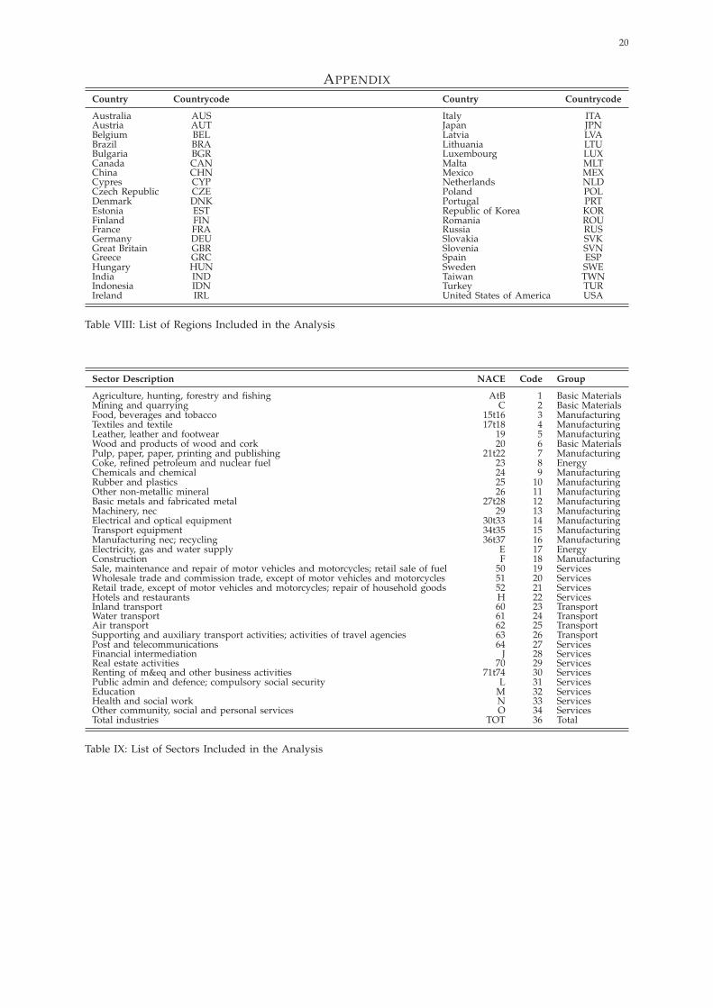
of the basic data. The dataset covers 40 regions (27 EU countries and 13 other majorcountries), which together account for approximately 85 % of world’s GDP in 2006.The WIOD data is disaggregated in 35 industries and provides detailed informationon primary (raw materials), secondary (manufacturing) as well as tertiary (services)sectors. In addition, it offers annual data which ranges from 1995 to 2009. Beside itsbroad country coverage, detailed sectoral disaggregation and time period character,the dataset has another important feature: it covers various aspects of economicactivity and for example involves accounts for energy and environmental issues orsocioeconomic and bilateral trade data. Employing the WIOD dataset in our esti-mation process involves three main benefits. We can estimate substitution elasticitiesusing one consistent dataset and do not have to merge potentially incompatible data.The comprehensive sectoral coverage of WIOD allows us to estimate substitutionelasticities for a broad set of sectors. Last but not least, for the first time we canderive elasticities from the same data which researchers can use also to calibratetheir simulations.In our analysis, we use in particular the WIOD Socio-Economic Accounts (SEA files)and the WIOD Energy Use tables (EU files). Taken together, they form a balancedpanel covering 40 regions and 34 sectors plus an economy-wide sector aggregate overa period of 15 years (1995 to 2009) and include detailed information on production in-and outputs.3 More specifically WIOD supplies us with data regarding the numberof total hours worked by persons engaged for the independent variable labour L,capital stock for the independent variable K , gross value added at basic prices for theindependent variable value added VA, intermediate inputs at purchasers’ prices forthe independent variable materials M, gross energy use for the independent variableenergy E and finally gross output at basic prices for the dependent variable outputY. Even though WIOD includes data up to the year 2009, in order to avoid drawingconclusions from a period of economic turmoil we drop the years 2008 and 2009for our analysis and focus on the period from 1995 to 2007. For the estimation, allmonetary values have been transformed to U.S. Dollars using the Penn World Table(Heston et al. , 2011) and are reported at 1995 prices. Energy is in Terajouls. Labouris given in million hours worked. Table I gives an overview of the variables usedin the estimation process. A complete list of the regions and sectors covered by thisanalysis is given in the Appendix.
Variable Definition Source Unit
Output Gross output at basic prices WIOD SEA Files million 1995 USDCapital Fixed capital stock WIOD SEA Files million 1995 USDLabour Total hours worked by persons engaged WIOD SEA Files million hoursValue Added Gross value added at basic prices WIOD SEA Files million 1995 USDEnergy Gross energy use WIOD EU Files TerajoulsMaterials Gross output at basic prices WIOD SEA Files million 1995 USD
Table I: List of Variables used in the Estimation
3 While originally the WIOD dataset features information for 35 sectors, entries for the sector privatehouseholds with employed persons remain empty in the SEA and EU files. Consequently we undertake theanalysis only for the 34 remaining sectors plus the economy-wide sector total.

6
B. Estimation Procedure
CES functions are non-linear in parameters and hence parameters can initially notbe estimated using standard non-linear estimation techniques. For this reason anddue to the so far rather tricky implementation of non-linear estimation procedures,most researchers estimating elasticities of substitution within a CES framework workwith CES functions that have been linearised in some form or the other. Thereby, theso-called Kmenta approximation (Kmenta , 1967) has been very popular. However,the original CES function cannot be linarised analytically and using approximationmethods to linearise the CES function can have drawbacks. Kmenta (1967) himselfnotes that if in the production function under investigation the input ratio as wellas the elasticity of substitution are either very high or very low, his approximationmethod may not perform well. Maddala and Kadane (1967) and Thursby and Lovell(1978) confirm this problem and shows that the standard Kmenta procedure may notlead to reliable estimates of parameters in a CES framework.To avoid issues related to Kmenta approximations without having to use cumbersomenon-linear estimation procedures, researchers also make use of the cost functionapproach (e.g. van der Werf , 2008; Okagawa and Ban , 2008). Thereby one can takeadvantage of the cost function associated with a specific production function andderive a linear system of equations from the corresponding optimal input demand.This can subsequently be used to estimate the function coefficients in question.But this approach requires comprehensive price data, which in most cases is ratherdifficult to come by, especially when undertaking sector specific analysis.In contrast to the majority of other studies investigating the substitutability of inputswithin a CES production structure, we estimate substitution elasticities directly fromthe CES production function and primarily building non-linear least-squares esti-mation procedures. Thereby we employ a set of different optimisation algorithms,namely the Levenberg-Marquardt algorithm (LM) (Marquardt , 1963), PORT routines(Gay , 1990), the Differential Evolution algorithm (DE) (Storn and Price , 1997; Priceet al. , 2005), Nelder-Mead routines (NM) (Nelder and Mead , 1965), the SimulatedAnnealing algorithm (SANN) (Kirkpatrick et al. , 1987; Cerny , 1985) and the socalled BFGS algorithm (Broyden , 1970; Fletcher , 1970; Goldfarb , 1970; Shanno ,1970). In some estimation runs we make use of starting values compiled by means ofa preceding grid search for the substitution parameter ρ involving LM.4 A detailedoverview of all the estimations we run is given in Table X in the Appendix. However,after having shown that except for SANN and DE our results are robust with regardto the choice of the employed optimisation algorithm, we continue our analysis onthe basis of the estimation process producing the best fit to the our data. Id estestimations relying on LM and PORT with starting values.For the actual estimation process we use the programming environment R withthe package micEconCES developed by Henningsen and Henningsen (2011). Butthe micEconCES package in its current version only allows to estimate parametersfor a two-level nested CES production function. Yet we would like to derive thesubstitution elasticities for a three-level nested CES function. To overcome this lim-
4 For more information on how adequate starting values are derived applying a preceding grid search, theinterested reader is kindly referred to Henningsen and Henningsen (2011).

7
itation, we benefit from the separability implied by the CES framework and splitthe originally three-level nested KLEM CES function we would like to investigategiven by Equation (5) into two individual CES functions. Accordingly we estimatethe substitution elasticities first for the non-nested CES function
VAt = γKLetλ(
αKL(Kt)−ρKL + (1− αKL) (Lt)
−ρKL) 1−ρKL , (7)
with the substitution elasticity σKL = 11+ρKL
. Subsequently we do the same for thetwo-level CES function
Yt = γKLEMetλ (αKLEM(Mt)−ρKLEM + (1− αKLEM)
((αKLE(Et)
−ρKLE+
(1− αKLE) (VAt)−ρKLE
) 1−ρKLE
)−ρKLEM) 1−ρKLEM
,(8)
with the substitution elasticities σKLE = 11+ρKLE
and σKLEM = 11+ρKLEM
. Taken together,Equation (7) and Equation (8) represent the overall CES function in question, whereas,as already indicated by Equation (5), Equation (7) is the bottom nest and Equation(8) corresponds to the middle and upper nests of the production function underinvestigation.The substitution elasticities are estimated specifically for each of the 34 sectors andone sector aggregate representing the total of all industries available in the WIODdataset. Thereby, we first pool all sectoral data across all regions. At a later stage wethen evaluate if input substitutability varies across regions. As indicated by Equation(7) and (8), initially we assume that elasticities are constant over time. Hence, inour setting technological progress can only take place through changes in overallproductivity. Though, this assumption is relaxed at a later stage.
IV. ESTIMATION RESULTS
Unsurprisingly, the estimates for the substitution parameters ρKL, ρKLE and ρKLEMand hence for σKL, σKLE and σKLEM differ across different estimation processes. Butall in all and in view of the respective standard errors, deviations are rather minor.Nevertheless we observe a small divergence between gradient-based local optimi-sation algorithms (BFGS, LM and PORT) and algorithms targeting global minima(e.g. NM). Robustness across estimation techniques decreases for smaller estimatedvalues of ρKL, ρKLE and ρKLEM and increases when adequate starting values from aprior grid search are used in the estimation process. The SANN, DE and in partsCG technique however are exceptions and lead to notable different results in severalcases, mainly suggesting smaller values for ρKL, ρKLE and ρKLEM than other methods.Convergence is tends also to be an issue when applying these solvers. Given theoverall robustness of the different estimations, we choose to continue our analysison the basis of only one estimation process. Evaluated on the basis of R-squared,the estimations relying on PORT routines or LM and BFGS methodologies performbest. Without starting values from a preceding grid search, CG and DE generatesthe poorest fit. When using starting values, CG appears to be the least powerful

8
method. Furthermore, by the same measure, estimations using starting values froma preceding grid search generally have a better fit than estimations without. Thisholds true for the investigation of Equation (7) as well as for Equation (8). Giventhe benefit of the usage of starting values and on the whole very similar estimationresults, in the following we focus on the estimations with the best fit to the data,id est estimations relying on PORT routines and which use starting values. Thecorresponding estimation results for the substitution parameter ρ for the time period1995 to 2007 with pooled data including all regions are summarised in Table II. Notethat for the bottom nest of sector 8 (coke, refined petroleum and nuclear fuel) we donot achieve convergence for any acceptable convergence criteria and do not report avalue for ρKL. Moreover, some of the estimates for ρ feature high standard deviations,these estimates are reported in brackets.
Sector N ρKL-Est. Std. Dev. ρKLE-Est. Std. Dev. ρKLEM-Est. Std. Dev.
1 520 -0.0652 0.0691 1.7926 0.8193 -0.3981 0.07472 520 0.2696 0.1283 (0.6173) >10 5.8104 1.80303 520 3.5627 1.1909 (3.6182) >10 -0.8772 0.25894 520 8.6122 4.2814 2.3552 1.1856 0.7798 0.10875 507 -1.6696 0.2706 3.4489 1.1924 0.9046 0.10426 520 7.3715 4.8299 (5.3491) >10 -1.1113 0.11477 520 10.1202 4.5846 2.2040 2.2719 0.8621 0.19888 502 NA -0.8024 4.4814 1.4299 0.30989 520 3.0891 0.4629 0.2873 0.2080 0.1431 0.267510 520 7.6535 2.1274 3.2905 0.4920 0.5610 0.145911 520 4.1269 0.9708 2.7814 4.4653 -0.0404 0.105712 520 4.5200 1.2438 -0.0880 0.1482 6.6645 0.879113 520 1.0962 0.1476 (2.6770) >10 -1.0707 0.103914 520 6.8617 5.5543 5.1445 2.4021 -1.6300 0.175315 520 4.4527 0.7621 (3.2122) >10 1.0076 0.271316 520 3.2720 0.5253 (9.1267) >10 -0.6243 0.116217 520 -1.2951 0.4679 1.3441 0.2532 0.4590 0.122118 520 4.7623 1.1559 (3.3779) >10 0.6699 0.226319 482 -1.1464 0.4433 (3.3588) >10 0.6339 0.141320 520 11.0342 4.6822 1.9928 2.9571 1.3476 0.090621 520 (18.7635) >10 (6.2982) >10 -0.1299 0.075522 520 13.9728 4.4939 0.6246 1.5113 0.6322 0.152023 520 6.2963 0.9537 2.7383 1.1057 0.1031 0.184024 506 -0.7027 0.1219 -1.6242 0.1339 0.6856 0.185825 519 3.3042 1.0377 2.1739 0.6831 -0.1913 0.077826 520 2.8367 0.4624 1.2960 0.2650 0.6695 0.034827 520 -0.5790 0.2753 (19.4998) >10 -0.6906 0.339828 520 4.5632 1.0965 (14.3869) >10 -0.9412 0.172729 516 2.2850 0.3494 -0.0524 0.1539 0.1093 0.108930 520 3.0716 0.3976 3.4990 1.1617 0.4070 0.226431 507 4.4847 1.2736 2.2639 1.6622 2.0595 0.258232 520 -1.7683 3.6457 1.4266 0.8185 -0.6047 0.051233 520 0.7311 0.1222 (7.6346) >10 -0.3502 0.053634 520 5.0364 2.7887 (3.1208) >10 0.4730 0.240836 520 6.4792 1.1071 1.9972 0.5056 -0.3195 0.1747
Table II: Estimation Results for ρ (Unrestricted PORT Routine with Starting Values, 1995-2007, all Regions)
For several sectors ρKL < 1, ρKLE < 1 or ρKLEM < 1 and thus violate the basicassumptions of the standard CES framework which requires σ ≥ 0 respectivelyρ ≥ −1. While so far we have applied an unrestricted estimation approach, thisindicates the need to incorporate the three parameter constraints implied by the CESframework γ > 0, 0 ≥ α ≥ 1 and σ ≥ 0 into our estimations. Table III summarises theresults for ρ when applying the restricted estimation. The corresponding results forσ are given in Table XI in the Appendix. For obvious reasons the fit for the restrictedmodel is not as good as before and again we do not achieve convergence for thebottom nest of sector 8. For six out of the 105 estimated elasticities, the conditionthat ρ ≥ −1 is binding. This could be an indication that for a small set of sectors,

9
the assumption of CES production structures provides only a poor fit to the actualprevailing production structure of these sectors. However, as for the big majority ofsectors and nests our estimation results seem to be reliable with regard to fit to thedata and standard deviations, and as the usage of of CES functions has proven to bevery popular in particular in CGE models, we proceed with our estimation processand continue including the constraints on γ, α and σ given by the CES framework.
Sector N ρKL-Est. Std. Dev. ρKLE-Est. Std. Dev. ρKLEM-Est. Std. Dev.
1 520 -0.0652 0.0691 1.5202 0.6513 0.0201 0.08752 520 0.2696 0.1283 1.3936 >10 3.5275 0.78143 520 3.5627 1.1909 4.2954 5.9377 0.5956 0.27644 520 8.6122 4.2814 2.6266 0.8898 0.7009 0.10665 507 -1.0000 0.1456 4.2824 1.1147 0.7887 0.09896 520 7.3715 4.8299 3.8764 1.5318 0.4029 0.16497 520 7.6868 2.6765 2.9515 1.5165 0.5129 0.18718 502 NA -1.0000 5.8118 1.4086 0.31129 520 3.2330 0.4957 0.3942 0.2231 0.0600 0.262510 520 7.6535 2.1274 4.4137 0.6568 0.4711 0.136411 520 4.1269 0.9708 3.0187 2.5446 0.2388 0.113412 520 4.5200 1.2438 -0.0055 0.1417 8.0932 1.091113 520 1.0962 0.1476 4.0343 1.2505 0.8336 0.205514 520 9.0265 9.6388 -0.0528 0.0900 0.5583 >1015 520 4.4527 0.7621 5.2611 3.8258 1.6428 0.307716 520 3.2720 0.5253 4.7058 2.0801 0.8868 0.151317 520 -1.0000 0.3691 1.1978 0.2380 0.4700 0.124218 520 4.7623 1.1559 5.7383 >10 0.6273 0.223319 482 -1.0000 0.3675 5.5439 9.5810 0.6571 0.143720 520 9.1375 3.1941 3.0928 2.5246 1.2898 0.089021 520 16.9923 9.8950 3.1064 1.5105 0.2890 0.086622 520 11.3644 3.0463 3.6164 2.3832 0.5994 0.141623 520 6.2963 0.9537 1.3576 3.3938 3.5116 0.380124 506 -0.7027 0.1219 -0.2131 0.0837 1.2093 0.288425 519 3.2201 0.9924 1.6778 0.5826 -0.0299 0.085226 520 2.8593 0.4695 1.5706 0.2701 0.7223 0.038227 520 -0.5816 0.2768 5.5188 >10 0.4779 0.497828 520 4.5632 1.0965 10.6398 >10 0.9370 0.361329 516 2.2436 0.3415 0.4655 0.1014 0.1930 >1030 520 3.0716 0.3976 4.5351 1.3563 0.5918 0.235831 507 4.4847 1.2736 1.0137 0.2113 -1.0000 >1032 520 -1.0000 1.2390 6.7918 4.5896 -0.0132 0.075633 520 0.7311 0.1222 5.4437 2.7086 0.2432 0.071934 520 5.0364 2.7887 3.6985 >10 0.4987 0.246136 520 6.7382 1.1876 1.6383 0.4412 -0.1277 0.1934
Table III: Estimation Results for ρ (Restricted PORT Routine with Starting Values, 1995-2007, all Regions)
Given our estimates, we continue and investigate whether the common simplificationof using Cobb-Douglas or Leontief functions in CGE models can be rejected by ourestimation results. Table IV presents our findings to this regard, sectors with noconvergence or binding restrictions for ρ are marked with NA.

10
Sector H0: σKL = 0 H0: σKL = 1 H0: σKLE = 0 H0: σKLE = 1 H0: σKLEM = 0 H0: σKLEM = 11 <0.01 <0.01 <0.01 <0.01 <0.01 <0.012 <0.01 <0.01 <0.01 <0.013 <0.01 <0.01 <0.01 <0.01 <0.01 <0.014 <0.01 <0.01 <0.01 <0.01 <0.01 <0.015 NA NA <0.01 <0.01 <0.01 <0.016 <0.01 <0.01 <0.01 <0.01 <0.01 <0.017 <0.01 <0.01 <0.01 <0.01 <0.01 <0.018 NA NA NA NA <0.01 <0.019 <0.01 <0.01 <0.01 <0.01 <0.01 <0.0110 <0.01 <0.01 <0.01 <0.01 <0.01 <0.0111 <0.01 <0.01 <0.01 <0.01 <0.01 <0.0112 <0.01 <0.01 <0.01 <0.01 <0.0113 <0.01 <0.01 <0.01 <0.01 <0.01 <0.0114 <0.01 <0.01 <0.01 <0.0115 <0.01 <0.01 <0.01 <0.01 <0.01 <0.0116 <0.01 <0.01 <0.01 <0.01 <0.01 <0.0117 NA NA <0.01 <0.01 <0.01 <0.0118 <0.01 <0.01 <0.01 <0.01 <0.01 <0.0119 NA NA <0.01 <0.01 <0.01 <0.0120 <0.01 <0.01 <0.01 <0.01 <0.01 <0.0121 <0.01 <0.01 <0.01 <0.01 <0.01 <0.0122 <0.01 <0.01 <0.01 <0.01 <0.01 <0.0123 <0.01 <0.01 <0.01 <0.01 <0.01 <0.0124 <0.01 <0.01 <0.01 <0.01 <0.01 <0.0125 <0.01 <0.01 <0.01 <0.01 <0.01 <0.0126 <0.01 <0.01 <0.01 <0.01 <0.01 <0.0127 <0.01 <0.01 <0.01 <0.01 <0.01 <0.0128 <0.01 <0.01 <0.01 <0.01 <0.01 <0.0129 <0.01 <0.01 <0.01 <0.0130 <0.01 <0.01 <0.01 <0.01 <0.01 <0.0131 <0.01 <0.01 <0.01 <0.01 NA NA32 NA NA <0.01 <0.01 <0.01 <0.0133 <0.01 <0.01 <0.01 <0.01 <0.01 <0.0134 <0.01 <0.01 <0.01 <0.01 <0.01 <0.0136 <0.01 <0.01 <0.01 <0.01 <0.01 <0.01
Table IV: Evaluation of Cobb-Douglas and Leontief Specification for CGE models (two-sided p-values for H0)
For all three nests the assumption of a Cobb-Douglas function (σKL = 1, σKLE = 1or σKLEM = 1) can be dismissed for almost all sectors. A similar picture emerges forthe assumption of a Leontief functional form (σKL = 0, σKLE = 0 or σKLEM = 0). Tobe exact, in the bottom nest the Leontief and the Cobb-Douglas framework must berejected for the all sectors. While in the middle nest the assumption of a Leontief-likeproduction structure can not be discarded for sector 2 which represents the miningand quarrying industry, a Cobb-Douglas production function can not be excludedin sectors 2 and 12 (basic metals and fabricated metal). A Leontief framework inthe top nest can be rejected for all sectors but sectors 14 (electrical and opticalequipment) and 29 (real estate activities). The same hold true for a Cobb-Douglasproduction structure. Overall, this strongly suggests that a simplified approach to thechoice of substitution elasticities including only Cobb-Douglas or Leontief productionfunctions is not appropriate and will eventually lead to misguiding results of anycounterfactual analysis.Table V compares the result of our estimations to the findings of Okagawa and Ban(2008), van der Werf (2008) and Kemfert (1998). It must be noted however thatfor several reasons a direct comparison of the results is difficult. First, non of thestudies uses the same data. Second, all of researchers undertake estimations for adifferent set of sectors. Hence their findings can only be compared on the basis of aspecific (possibly arbitrary) sectoral mapping. Third, Okagawa and Ban (2008) as wellas Kemfert (1998) do not supply information on the standard error of their results.Fourth, the studies employ different estimation techniques. As a consequence we cannot truly test whether our results differ from their findings. Nevertheless, keepingthis in mind, we can observe that at large our estimates for σKL, σKLE and σKLEM are

11
neither consistently higher nor smaller than the substitution elasticities supplied byOkagawa and Ban . With few exceptions, compared to the elasticities derived by vander Werf (2008) or Kemfert (1998), our estimates seem to be systematically smaller.Besides the more fundamental issues mentioned above, there are potentially severalreasons for the differences between our estimates and those from other studies. Ourdata may not be up to the task or our choice of variables as illustrated in Table I isinappropriate. However, as Okagawa and Ban (2008), van der Werf (2008) as wellas Kemfert (1998) use similar data and variables, these issues do not immediatelysuggest themselves as the main reasons for the deviations. Alternatively, the devia-tions may arise due to the usage of different estimation approaches, in particular withregard to linear or and non-linear estimation techniques. In effect, while Okagawaand Ban (2008) and van der Werf (2008) estimate substitution elasticities using linearestimation processes and applying a cost function approach, the elasticities derivedin this paper stem from a non-linear estimation process using the original functionalform of a CES production function. Only Kemfert (1998) applies also a non-linearestimation to the problem.

12
Sector
σK
L-Est.
σK
LE-Est.
σK
LEM-Est.
Own
OB
WK
Own
OB
WK
Own
OB
WK
Own
OB
1AGR
1.0697
0.023
0.3968
0.516
0.9803
0.392
2MIN
Ston
eandearth
0.7876
0.139
0.21
0.4178
0.553
0.56
0.2209
0.729
3FO
OFo
odandtob.
Food
0.2192
0.382
0.4597
0.66
0.1888
0.395
0.399
0.78
0.6267
0.329
4TE
XTextilesetc.
0.1040
0.161
0.2737
0.2757
0.637
0.2944
0.5879
0.722
5(Inf)
0.1893
0.5591
6WOO
0.1195
0.087
0.2051
0.456
0.7128
0.695
7PP
PPa
peretc.
Paper
0.1151
0.381
0.4103
0.35
0.2531
0.211
0.4489
0.73
0.6610
0.187
8NA
(Inf)
0.4152
9CHM
Chemical
indu
stry
0.2362
0.334
0.37
0.7172
-0.065
0.97
0.9434
0.848
100.1156
0.1847
0.6798
11NMM
Non
-metallic
minerals
0.1950
0.358
0.4541
0.2488
0.411
0.2546
0.8072
0.306
12BM
EBa
sismetals
Iron
0.1812
0.22
0.619
0.5
1.0055
0.644
0.6454
0.4
0.1100
1.173
13MAC
0.4771
0.295
0.1986
0.292
0.5454
0.13
14EE
Q0.0997
0.163
1.0557
0.524
0.6417
0.876
15TE
QTransporteq.
Vehicle
0.1834
0.144
0.4638
0.1
0.1597
0.519
0.1705
0.35
0.3784
0.548
16MAN
0.2341
0.046
0.1753
0.529
0.5300
0.406
17EG
W(Inf)
0.46
0.4550
0.256
0.6803
-0.04
18CON
Con
struction
0.1735
0.065
0.2242
0.1484
0.529
0.2892
0.6145
1.264
19(Inf)
0.1528
0.6034
200.0986
0.2443
0.4367
210.0556
0.2435
0.7758
220.0809
0.2166
0.6252
23TR
N0.1371
0.31
0.4242
0.281
0.2217
0.352
24TR
N3.3637
0.31
1.2709
0.281
0.4526
0.352
25TR
N0.2370
0.31
0.3734
0.281
1.0308
0.352
26TR
N0.2591
0.31
0.3890
0.281
0.5806
0.352
27TE
L2.3901
0.37
0.1534
0.518
0.6766
0.654
28FB
S0.1798
0.264
0.0859
0.32
0.5163
0.492
290.3083
0.6823
0.8382
300.2456
0.1807
0.6282
310.1823
0.4966
(Inf)
32(Inf)
0.1283
1.0133
330.5777
0.1552
0.8044
34PS
E0.1657
0.316
0.2128
0.784
0.6673
0.902
360.1292
0.3790
1.1464
Non
-ferrous
-0.22
0.83
TableV:C
ompa
risonof
Results
(RestrictedPO
RTRou
tine
withStarting
Values,1995-2007,
allRegions),OB:
OkagawaandBa
n(2008),W
:van
derWerf(2008),K
:Kem
fert
(1998)

13
The time series character of our data allows us to engage in an additional analysisand makes it possible to investigate whether substitution elasticities change overtime. In the economic literature, technological progress within the CES framework ismainly understood as a change in input productivity and researchers focus primarilyon determining λ in Equation 4. But in principle the CES framework for productionfunctions leaves room for technological change affecting not only productivity butalso the substitutability between different production inputs. In this case a modifiedCES function which takes into account changes of the substitution parameter overtime and incorporates Hicks-neutral technological change would take the form:
y = γeλt
(∑
iαi(xi)
−ρt
) 1−ρt
. (9)
The textile industry at the end of the 18th century provides an excellent exampleof this form of technological change. As looms became more and more advanced,human labour could be replaced more easily in the production process. Eventuallythis had a huge effect on business and society in that period.Embarking on a simple approach, we test whether we can observe a change in inputsubstitutability over time by reestimating Equations (7) and (8) and comparing σ
for two different time periods (1995 to 1997 and 2005 to 2007). Table VI summarisesthe results to this regard. Note that for some sectors convergence or CES constraintissues arise when using a restraint time period, the respective sectors are markedwith an NA value. In the bottom, middle nest and top nest, the hypothesis that thesubstitution elasticities do not change over time can be rejected for about two thirds ofthe sectors under investigation. When evaluating a less stringent comparison betweenthe two periods, the picture becomes even clearer and we can reject a significantchange in input substitutability for all but a handful of sectors.5 To allow for amore detailed analysis investigating if there have been any structural changes ofthe substitution elasticities over time, we group the results in five groups dependingon the evaluated sector, namely Basic Materials, Energy, Manufacturing, Services andTransport, the underlying mapping is outlined in Table ?? in the Appendix. But evenwhen investigating only specific sectors groups, we do not observe any significantchanges over time. Moreover, for all sector groups, the hypothesis that there hasbeen an increase in elasticities has to be rejected equally often as the hypothesisthat elasticities have decreased. Hence our results suggest, that there has been nostructural change in elasticities over time. This implies also that changing substi-tution elasticities appear not to be a problem for our estimations, which originallyconsider the complete time period between 1995 to 2007. But nevertheless, the issue ispotentially important. As a consequence, in future research this particular dimensionof technological progress needs to be taken into account and should be investigatedwith more rigour. Ultimately this will require studying longer time periods as thoseunder investigation so far in studies on the substitutability of inputs and also aformalisation of the issue within the CES framework.
5 We assume that a significant change would imply a production structure changing from Leontief to CobbDouglas, i.e. a change resulting in |σ95−97 − σ05−07| > 1.

14
H0for
σK
L-Est.:
H0for
σK
LE-Est.:
H0for
σK
LEM-Est.:
Sector
σ 95−
97≤
σ 05−
07σ 9
5−97≥
σ 05−
07|σ 9
5−97−
σ 05−
07|>
1σ 9
5−97≤
σ 05−
07σ 9
5−97≥
σ 05−
07|σ 9
5−97−
σ 05−
07|>
1σ 9
5−97≤
σ 05−
07σ 9
5−97≥
σ 05−
07|σ 9
5−97−
σ 05−
07|>
11
<0.01
<0.01
<0.01
<0.01
<0.1
<0.01
2<0
.01
<0.01
<0.01
<0.01
3<0
.01
<0.01
<0.01
4<0
.01
<0.01
<0.01
<0.01
<0.01
5NA
NA
NA
NA
NA
NA
NA
NA
NA
6<0
.01
<0.01
<0.01
<0.01
7<0
.05
<0.01
<0.01
<0.01
<0.01
8NA
NA
NA
NA
NA
NA
<0.01
<0.01
9<0
.1<0
.01
<0.01
<0.01
<0.01
<0.01
10<0
.01
<0.01
<0.01
<0.01
11<0
.01
<0.01
<0.01
<0.01
<0.01
12<0
.05
<0.01
<0.01
<0.01
<0.01
<0.01
13<0
.01
<0.01
<0.01
<0.01
<0.01
<0.01
14<0
.01
<0.05
<0.05
15<0
.01
<0.01
<0.01
16<0
.01
<0.01
<0.01
<0.01
<0.01
<0.01
17NA
NA
NA
<0.01
<0.01
<0.01
18<0
.01
<0.01
<0.01
<0.05
<0.01
19NA
NA
NA
<0.01
<0.05
<0.01
20<0
.01
<0.01
<0.01
<0.01
21<0
.01
<0.01
<0.01
<0.01
<0.05
<0.01
22<0
.01
<0.01
<0.01
<0.01
<0.01
<0.01
23<0
.01
<0.01
<0.01
<0.01
<0.01
24<0
.01
<0.01
<0.01
<0.01
25<0
.01
<0.01
<0.01
<0.01
<0.01
<0.01
26<0
.01
<0.01
<0.01
<0.01
<0.01
<0.01
27<0
.01
28<0
.01
<0.01
<0.01
<0.01
<0.01
29<0
.01
<0.01
<0.01
<0.01
30<0
.05
<0.01
<0.01
<0.01
<0.01
<0.01
31<0
.01
<0.01
<0.05
<0.01
<0.01
<0.01
32NA
NA
NA
<0.01
<0.01
<0.01
<0.01
33<0
.01
<0.01
<0.01
<0.05
<0.01
34<0
.01
<0.1
<0.05
<0.01
36<0
.01
<0.01
<0.01
<0.01
<0.01
<0.01
TableVI:Com
parisonof
theSu
bstitution
Elasticities
forthePeriod
s1995-1997and2005-2007(RestrictedPO
RTRou
tine
withStarting
Values,allRegions,p
-valuesforH0)

15
Having investigated the variability of input substitutability over time, we next evalu-ate whether elasticities vary across regions. We apply a similar approach as before andcompare estimates for different regions with each other to test for regional variation.Although here we only present the results of a comparison between the estimatesfor the EU27 and the BRIC countries (Brazil, Russia, India and China), a similarpicture emerges when contrasting the results for countries with a high productivityto those featuring a relatively low productivity.6 Table ?? illustrates the results whencomparing estimation results for the EU27 with those for BRIC. Again, we do notachieve convergence for the bottom nest of sector 8 and in particular in the bottomnest several estimates are driven by the constraints of the CES framework. Theseestimates are marked with NAs. For all three nests, there is no significant changein input substitutability across regions for the large majority of sectors. Only for thegroups associated with service and manufacturing activities in the BRIC countries,we can not reject a higher input substitutability between the capital-labour-energycomposite and materials compared to estimates for the EU for a fair number of sec-tors. For the other two nests and sector groups, one can not conclude that elasticitiesare higher or lower in the EU compared to the BRIC countries and vice versa. Henceoverall, there appears to be no regional variation in elasticities of substitution.
6 For this analysis, we rank the countries under investigation according to their score in the index GDP perperson employed (constant 1990 PPP USD) from the World Bank

16
H0for
σK
L-Est.:
H0for
σK
LE-Est.:
H0for
σK
LEM-Est.:
Sector
σEU≤
σB
RIC
σEU≥
σB
RIC
|σ EU−
σB
RIC|>
1σ
EU≤
σB
RIC
σEU≥
σB
RIC
|σ EU−
σB
RIC|>
1σ
EU≤
σB
RIC
σEU≥
σB
RIC
|σ EU−
σB
RIC|>
11
<0.01
<0.01
<0.01
<0.01
<0.01
<0.01
2<0
.01
<0.01
<0.01
<0.01
<0.01
3<0
.01
<0.01
<0.05
<0.01
4<0
.01
<0.05
<0.01
<0.01
<0.01
5<0
.01
<0.01
<0.01
<0.01
<0.01
6<0
.01
<0.01
<0.05
<0.01
<0.01
<0.01
7NA
NA
NA
<0.01
<0.01
<0.01
<0.01
8NA
NA
NA
<0.01
<0.01
9NA
NA
NA
<0.01
<0.01
<0.01
<0.01
10NA
NA
NA
<0.01
<0.01
<0.01
11<0
.01
<0.05
<0.01
12<0
.01
<0.01
<0.01
<0.01
13<0
.01
<0.01
<0.01
14NA
NA
NA
<0.01
<0.01
15NA
NA
NA
<0.01
<0.01
<0.01
16<0
.01
<0.01
<0.01
<0.01
<0.01
17NA
NA
NA
<0.05
<0.01
18<0
.01
<0.01
<0.05
<0.01
<0.01
19<0
.01
<0.01
<0.01
<0.01
<0.01
<0.01
20NA
NA
NA
<0.01
<0.01
<0.01
21<0
.01
<0.01
<0.01
<0.01
<0.01
<0.01
22NA
NA
NA
<0.1
<0.01
<0.01
<0.01
23<0
.01
<0.01
<0.01
24NA
NA
NA
NA
NA
NA
<0.05
25<0
.01
<0.01
NA
NA
NA
26<0
.01
<0.01
<0.01
<0.01
<0.01
<0.01
27NA
NA
NA
<0.01
<0.01
<0.01
28<0
.01
<0.01
<0.1
<0.01
<0.01
<0.01
29<0
.01
<0.01
<0.01
<0.01
30<0
.01
<0.01
<0.01
<0.05
<0.01
31NA
NA
NA
<0.01
<0.01
<0.01
<0.01
32<0
.01
<0.01
<0.01
<0.01
<0.01
33<0
.01
<0.01
<0.05
<0.01
<0.01
<0.01
34NA
NA
NA
<0.01
<0.01
<0.01
<0.01
36<0
.01
<0.01
<0.05
<0.01
TableVII:C
ompa
risonof
theSu
bstitution
Elasticities
fortheRegions
EUandBR
IC(RestrictedPO
RTRou
tine
withStarting
Values,1997-2009,
p-values
forH0)

17
V. SUMMARY AND CONCLUSION
Elasticities, in particular substitution elasticities, are vital parameters for any micro-consistent economic model and crucially influence the results of counterfactual policyanalysis. But so far only few consistent estimates of elasticities exist. With this pa-per we aim at overcoming this problem. Building on a rich dataset based on theWIOD data, we systematically investigate input substitutability in a CES productionframework for a KLEM production structure using non-linear estimation procedures.On the basis of our estimations, we demonstrate that the common practice of usingCobb-Douglas or Leontief production functions in economic models must be rejectedfor the majority of sectors. This calls for a more elaborate approach with regard tosubstitution elasticities. In particular in response to this result, we provide a compre-hensive set of consistently estimated substitution elasticities covering a wide range ofdifferent sectors. Our results suggest additionally that no significant change in inputsubstitutability takes place over during the time period we consider. Hence for mostsectors we do not observe technological change through this channel. Although tech-nological progress in the form of changing substitution elasticities may potentially bean issue when studying longer time periods. Moreover, there is no significant regionalvariation in substitution elasticities across regions. By providing an exhaustive setof substitution elasticities and with our analysis of input substitutability over timeand across regions, we hope to make a valuable contribution to making instrumentsdesigned to evaluate policy measures ex-ante more reliable and support researchers aswell as policy makers in their efforts to find solutions for today’s challenges requiringregulative interventions.

18
REFERENCES
ARROW, K.J., CHENERY, H.B., MINHAS, B.S. and SOLOW, R.M. (1961): Capital-LaborSubstitution and Economic Efficiency, in: The Review of Economics and Statistics,Vol. 43, pp. 225-250.
BALISTRERI, E.J., MCDANIEL, C.A., and WONG, E.V. (2003): n estimation of USindustry-level capital-labor substitution elasticities: Support for Cobb-Douglas, in:The North American Journal of Economics and Finance, Vol. 14, pp. 343-356.
BÖHRINGER, C., RUTHERFORD, T.F., and WIEGARD, W. (2003): Computable GeneralEquilibrium Analysis: Opening a Black Box, in: ZEW Discussion Paper, No. 03-56.
BROWNING, M., HANSEN, L.P., and HECKMAN, J. J. (1999): Micro data and generalequilibrium models, in: Handbook of Macroeconomics, Vol. 1, Part A, Chapter 8,pp. 543-633.
BROYDEN, C.G. (1970): The Convergence of a Class of Double-rank MinimizationAlgorithms, in: Journal of the Institute of Mathematics and Its Applications, Vol. 6,pp. 76-90.
CASELLI, F. (2005): Accounting for Cross-Country Income Differences, in: Handbookof Economic Growth, Vol. 1, No. 1, Chapter 9, pp. 679-741.
CERNY, V. (1985): Thermodynamical approach to the traveling salesman problem: Anefficient simulation algorithm, in: Journal of Optimization Theory and Applications,Vol. 45, pp. 41-51.
DAWKINS, C., SRINIVASAN, T.N., WHALLEY, J., and HECKMAN, J. J. (2001): Calibra-tion, in: Handbook of Econometrics, Vol. 5, Chapter 58, pp. 3653-3703.
DEVARAJAN, S. and ROBINSON, S. (2002): The influence of computable generalequilibrium models on policy, in: TMD Discussion Paper.
FLETCHER, R. (1970): A New Approach to Variable Metric Algorithms, in: ComputerJournal, Vol. 13, pp. 317-322.
GAY, D.M. (1990): Usage Summary for Selected Optimization Routines, in: AT & TBell Laboratories.
GOLDFARB, D.A. (1970): A Family of Variable Metric Updates Derived by VariationalMeans, in: Mathematics of Computation, Vol. 24, pp. 23-26.
HENNINGSEN, A. and HENNINGSEN, G. (2002): Econometric Estimation of theConstant Elasticity of Substitution Function in R: Package micEconCES, in: FOIWorking Paper, No. 9.
HESTON, Alan, Robert SUMMERS and Bettina ATEN (2011): Penn World TablesVersion 7.0, by: Center for International Comparisons of Production, Income andPrices at the University of Pennsylvania, 2011.
JACOBY, H.D., REILLY, J.M., MCFARLAND, J.R., and PALTSEV, S. (2006): Technologyand technical change in the MIT EPPA model, in: Energy Economics, Vol. 28, pp.610-631.
KEMFERT, C. (1998): Estimated substitution elasticities of a nested CES productionfunction approach for Germany, in: Energy Economics, Vol. 20, pp. 249-264.
KIRKPATRICK, S., GELATT, C.D.J.., and VECCHI (1987): Optimization by simulatedannealing Computer vision: issues, problems, principles, and paradigms, in: Com-puter Vision: Issues, Problems, Principles, and Paradigms, Chapter 5, pp. 606-615.
KLUMP, R. and DE LA GRANDVILLE, O. (2000): Economic Growth and the Elasticity

19
of Substitution, in: The American Economic Review, Vol. 90(1), pp. 282–91.KMENTA, J. (1967): On Estimation of the CES Production Function, in: International
Economic Review, Vol. 8, pp. 180-189.LEÓN-LEDESMA, M. A., MCADAM, P. and WILLMAN, A. (2010): Identifying theElasticity of Substitution with Biased Technical Change, in: The American EconomicReview, Vol. 100, pp. 1330-1357.
MADDALA, G.S. and KADANE, J.B. (1967): Estimation of Returns to Scale and theElasticity of Substitution, in: Econometrica, Vol. 35, pp. 419-423.
MARQUETTI, A. and FOLEY, D. (2008): Extended Penn World Tables Version 3.0,http://homepage.newschool.edu/˜foleyd/epwt/
MANSUR, A.H. and WHALLEY, J. (1984): Numerical Specification of Applied Gen-eral Equilibrium Models: Estimation, Calibration and Data, in: Applied GeneralEquilibrium Analysis.
MARQUARDT, D.W. (1963): An Algorithm for Least-Squares Estimations of NonlinearParameters, in: Journal of the Society for Industrial and Applied Mathematics, Vol.11, pp. 431-441.
MCKITRICK, R.R. (1998): The econometric critique of computable general equilibriummodeling: the role of functional forms, in: Economic Modelling, Vol. 15, pp. 543-573.
NELDER, J. and MEAD, R. (1965): A Simplex Method for Function Minimization, in:The Computer Journal, Vol. 7, pp. 308-313.
OKAGAWA, A. and BAN, K. (2008): Estimation of substitution elasticities for CGEmodels, in: Discussion Papers in Economics and Business, No. 08-16.
PRICE, K.V., STORN, R.M., and LAMPINEN, J.A. (2005): Differential evolution: apractical approach to global optimization, Springer, Heidelberg, Germany.
SALTER W.E.G. (1966): Productivity and Technical Change, 2nd edition (1st edition1960), Cambridge University Press, Cambridge, UK.
SATO, K. (1967): A Two-Level Constant-Elasticity-of-Substitution Production Func-tion, in: The Review of Economic Studies, Vol. 34, pp. 201-218.
SHANNO, D.F. (1970): Conditioning of Quasi-Newton Methods for Function Mini-mization, in: Mathematics of Computation, Vol. 24, pp. 647-656.
SOLOW, R. M. (1956): A Contribution to the Theory of Economic Growth, in: TheQuarterly Journal of Economics, Vol. 70, pp. 65-94.
STORN, R. and PRICE K. (1997): Differential Evolution - A Simple and EfficientHeuristic for global Optimization over Continuous Spaces, in: Journal of GlobalOptimization, Vol. 11, pp. 341-359.
SUE WING, I. (2004): Computable General Equilibrium Models and Their Use inEconomy-Wide Policy Analysis: Everything You Ever Wanted to Know (But WereAfraid to Ask), in: MIT Technical Note, No. 6.
THURSBY, J.G. and LOVELL C.A.K. (1978): An Investigation of the Kmenta Approxi-mation to the CES Function, in: International Economic Review, Vol. 19, pp. 363-377.
VAN DER WERF, E. (2008): Production functions for climate policy modeling: Anempirical analysis, in: Energy Economics, Vol. 30, pp. 2964-2979.
VON WEIZSÄCKER, C.C. (1966): Tentative Notes on a Two Sector Model with InducedTechnical Progress, in: The Review of Economic Studies, Vol. 33, pp. 245-251.
20
APPENDIX
Country Countrycode Country Countrycode
Australia AUS Italy ITAAustria AUT Japan JPNBelgium BEL Latvia LVABrazil BRA Lithuania LTUBulgaria BGR Luxembourg LUXCanada CAN Malta MLTChina CHN Mexico MEXCypres CYP Netherlands NLDCzech Republic CZE Poland POLDenmark DNK Portugal PRTEstonia EST Republic of Korea KORFinland FIN Romania ROUFrance FRA Russia RUSGermany DEU Slovakia SVKGreat Britain GBR Slovenia SVNGreece GRC Spain ESPHungary HUN Sweden SWEIndia IND Taiwan TWNIndonesia IDN Turkey TURIreland IRL United States of America USA
Table VIII: List of Regions Included in the Analysis
Sector Description NACE Code Group
Agriculture, hunting, forestry and fishing AtB 1 Basic MaterialsMining and quarrying C 2 Basic MaterialsFood, beverages and tobacco 15t16 3 ManufacturingTextiles and textile 17t18 4 ManufacturingLeather, leather and footwear 19 5 ManufacturingWood and products of wood and cork 20 6 Basic MaterialsPulp, paper, paper, printing and publishing 21t22 7 ManufacturingCoke, refined petroleum and nuclear fuel 23 8 EnergyChemicals and chemical 24 9 ManufacturingRubber and plastics 25 10 ManufacturingOther non-metallic mineral 26 11 ManufacturingBasic metals and fabricated metal 27t28 12 ManufacturingMachinery, nec 29 13 ManufacturingElectrical and optical equipment 30t33 14 ManufacturingTransport equipment 34t35 15 ManufacturingManufacturing nec; recycling 36t37 16 ManufacturingElectricity, gas and water supply E 17 EnergyConstruction F 18 ManufacturingSale, maintenance and repair of motor vehicles and motorcycles; retail sale of fuel 50 19 ServicesWholesale trade and commission trade, except of motor vehicles and motorcycles 51 20 ServicesRetail trade, except of motor vehicles and motorcycles; repair of household goods 52 21 ServicesHotels and restaurants H 22 ServicesInland transport 60 23 TransportWater transport 61 24 TransportAir transport 62 25 TransportSupporting and auxiliary transport activities; activities of travel agencies 63 26 TransportPost and telecommunications 64 27 ServicesFinancial intermediation J 28 ServicesReal estate activities 70 29 ServicesRenting of m&eq and other business activities 71t74 30 ServicesPublic admin and defence; compulsory social security L 31 ServicesEducation M 32 ServicesHealth and social work N 33 ServicesOther community, social and personal services O 34 ServicesTotal industries TOT 36 Total
Table IX: List of Sectors Included in the Analysis

21
Region Time Period Solver Starting Values Restricted Coefficients Technological Progressfrom Grid Search (
γ ≥ 0, 0 ≤ αi ≤ 1,∑ni=1 αi , ρ ≥ −1
) (Hicks-neutral)All Countries 1995 to 2007 BFGS no no yes
yes no yesDE no no yes
no yes yesKM no no noLM no no yes
yes no yesno no noyes no no
NM no no yesyes no yes
PORT no no yesno yes yesyes no yesyes yes yesno no nono yes noyes no noyes yes no
SANN no no yesyes no yes
All Countries 1995 to 1997 PORT yes yes yes
All Countries 2005 to 2007 PORT yes yes yes
All Countries 2008 to 2009 PORT yes yes yes
High Productivity 1995 to 2007 PORT yes yes yes
Low Productivity 1995 to 2007 PORT yes yes yes
EU 1995 to 2007 PORT yes yes yes
Western 1995 to 2007 PORT yes yes yes
ROW 1995 to 2007 PORT yes yes yes
BRIC 1995 to 2007 PORT yes yes yes
Table X: List of Estimations Procedures Included in the Analysis

22
Sector N σKL-Est. Std. Dev. σKLE-Est. Std. Dev. σKLEM-Est. Std. Dev.
1 520 1.0697 0.0791 0.3968 0.1026 0.9803 0.08412 521 0.7876 0.0796 0.4178 >10 0.2209 0.03813 522 0.2192 0.0572 0.1888 0.2117 0.6267 0.10864 523 0.1040 0.0463 0.2757 0.0677 0.5879 0.03695 524 (Inf) NA 0.1893 0.0399 0.5591 0.03096 525 0.1195 0.0689 0.2051 0.0644 0.7128 0.08387 526 0.1151 0.0355 0.2531 0.0971 0.6610 0.08178 527 NA (Inf) NA 0.4152 0.05379 528 0.2362 0.0277 0.7172 0.1148 0.9434 0.233710 529 0.1156 0.0284 0.1847 0.0224 0.6798 0.063011 530 0.1950 0.0369 0.2488 0.1576 0.8072 0.073912 531 0.1812 0.0408 1.0055 0.1433 0.1100 0.013213 532 0.4771 0.0336 0.1986 0.0493 0.5454 0.061114 533 0.0997 0.0959 1.0557 0.1003 0.6417 >1015 534 0.1834 0.0256 0.1597 0.0976 0.3784 0.044116 535 0.2341 0.0288 0.1753 0.0639 0.5300 0.042517 536 (Inf) NA 0.4550 0.0493 0.6803 0.057518 537 0.1735 0.0348 0.1484 0.2952 0.6145 0.084319 538 (Inf) NA 0.1528 0.2237 0.6034 0.052320 539 0.0986 0.0311 0.2443 0.1507 0.4367 0.017021 540 0.0556 0.0306 0.2435 0.0896 0.7758 0.052122 541 0.0809 0.0199 0.2166 0.1118 0.6252 0.055423 542 0.1371 0.0179 0.4242 0.6106 0.2217 0.018724 543 3.3637 1.3787 1.2709 0.1352 0.4526 0.059125 544 0.2370 0.0557 0.3734 0.0813 1.0308 0.090526 545 0.2591 0.0315 0.3890 0.0409 0.5806 0.012927 546 2.3901 1.5812 0.1534 0.3779 0.6766 0.227928 547 0.1798 0.0354 0.0859 0.1241 0.5163 0.096329 548 0.3083 0.0325 0.6823 0.0472 0.8382 >1030 549 0.2456 0.0240 0.1807 0.0443 0.6282 0.093131 550 0.1823 0.0423 0.4966 0.0521 (Inf) NA32 551 (Inf) NA 0.1283 0.0756 1.0133 0.077733 552 0.5777 0.0408 0.1552 0.0652 0.8044 0.046534 553 0.1657 0.0765 0.2128 1.0670 0.6673 0.109636 554 0.1292 0.0198 0.3790 0.0634 1.1464 0.2541
Table XI: Estimation Results for σ (Restricted PORT Routine with Starting Values, 1995-2007, all Regions)