suffix tree and suffix array r9292202 5 brain chen r9254802 8 pluto chang
TRANSCRIPT

Suffix Tree and Suffix Array
R92922025 Brain Chen
R92548028
Pluto Chang
Outline
Motivation Exact Matching Problem Suffix Tree
Building issues Suffix Array
Build Search Longest common prefixes
Extra topics discussion Suffix Tree VS. Suffix Array

•Text search•Need fast searching algorithm(with low space cost)
•DNA sequences and protein sequences are too large to search by traditional algorithms•Some improved algorithms perform efficiently
•KMP, BM algorithms for string matching•Suffix Tree with linear construction and searching time•Suffix Array with Suffix Tree based construction
Motivation

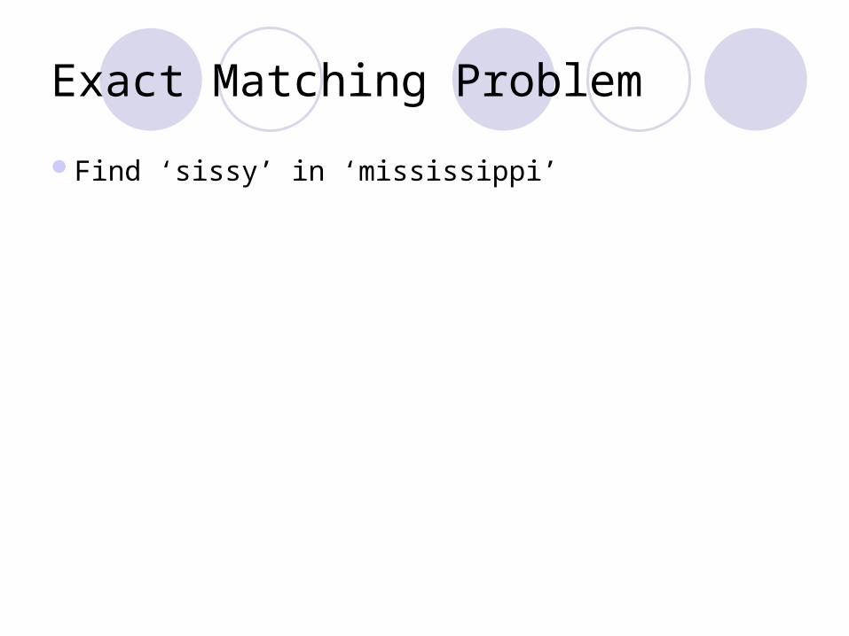
Exact Matching Problem
Find ‘ssi’ in ‘mississippi’
poulin at cs_ualberta_ca http://www.cs.ualberta.ca/~poulin/

Exact Matching ProblemFind ‘ssi’ in ‘mississippi’

Exact Matching ProblemFind ‘ssi’ in ‘mississippi’
s
si

Exact Matching ProblemFind ‘ssi’ in ‘mississippi’
s
si
Every leaf below this pointin the tree marks the startinglocation of ‘ssi’ in ‘mississippi’.(ie. ‘ssissippi’ and ‘ssippi’)
ssippi
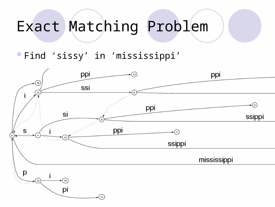
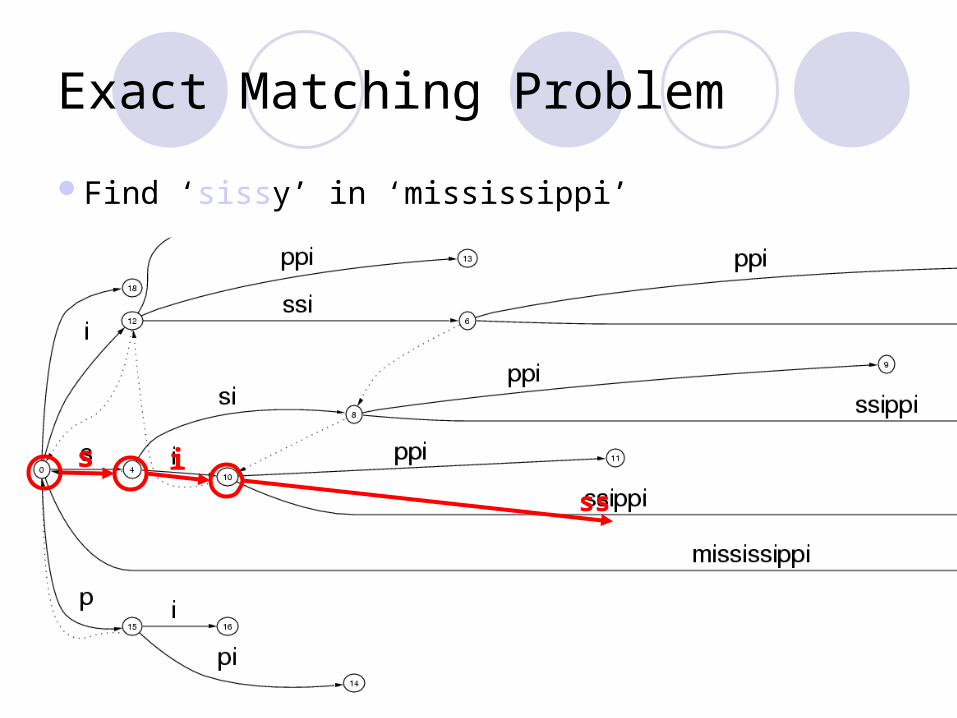
Exact Matching Problem
Find ‘sissy’ in ‘mississippi’
Exact Matching Problem
Find ‘sissy’ in ‘mississippi’
Exact Matching Problem
Find ‘sissy’ in ‘mississippi’
s i
ss

Exact Matching Problem
Find ‘sissy’ in ‘mississippi’
s i
ss
Exact Matching Problem
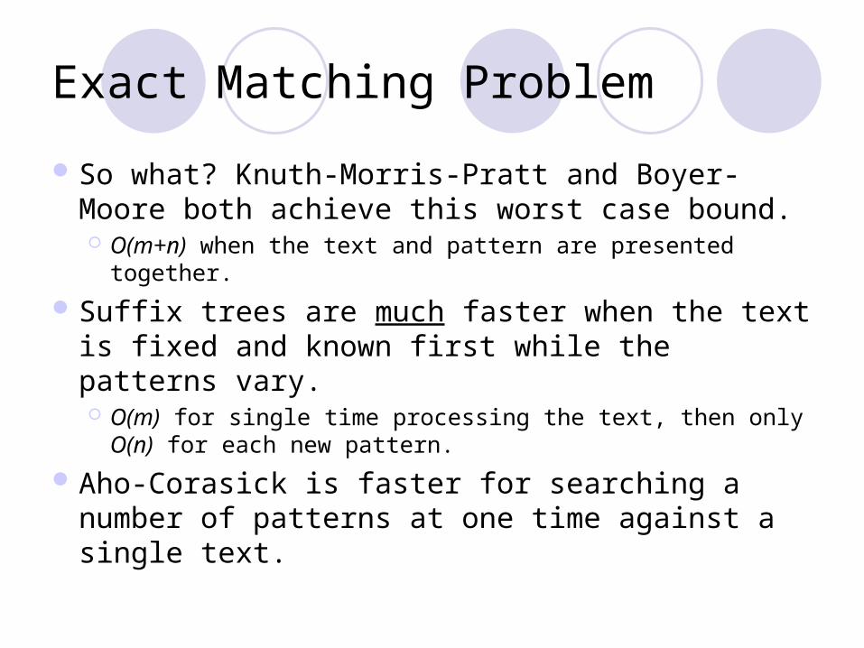
So what? Knuth-Morris-Pratt and Boyer-Moore both achieve this worst case bound. O(m+n) when the text and pattern are presented
together.
Suffix trees are much faster when the text is fixed and known first while the patterns vary. O(m) for single time processing the text, then only O(n)
for each new pattern.
Aho-Corasick is faster for searching a number of patterns at one time against a single text.

Boyer-Moore Algorithm
For string matching(exact matching problem)
Time complexity O(m+n) for worst case and O(n/m) for absense
Method: backward matching with 2 jumping arrays(bad character table and good suffix table)

What are suffix arrays and trees?• Text indexing data structures• not word based• allow search for patterns or • computation of statistics
Important Properties• Size• Speed of exact matching• Space required for construction• Time required for construction

Suffix Tree
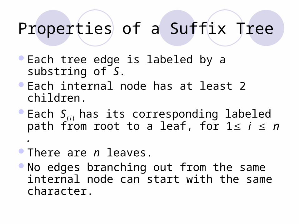
Properties of a Suffix Tree
Each tree edge is labeled by a substring of S.
Each internal node has at least 2 children.Each S(i) has its corresponding labeled
path from root to a leaf, for 1 i n .There are n leaves.No edges branching out from the same
internal node can start with the same character.

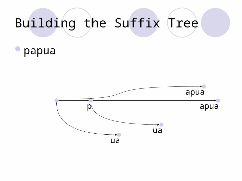
Building the Suffix Tree
How do we build a suffix tree?while suffixes remain:
add next shortest suffix to the tree
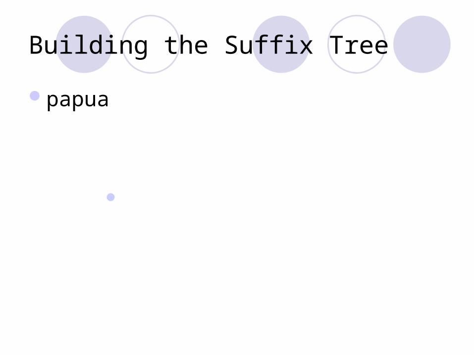
Building the Suffix Tree
papua

Building the Suffix Tree
papua
papua

Building the Suffix Tree
papua
papua
apua

Building the Suffix Tree
papua
apua
apua
p
ua
Building the Suffix Tree
papua
apua
apua
p
uaua

Building the Suffix Tree
papua
apua
pua
p
uaua
a

Building the Suffix Tree
papua
apua
pua
p
uaua
a

Building the Suffix Tree
How do we build a suffix tree?while suffixes remain:
add next shortest suffix to the tree
Naïve method - O(m2) (m = text size)
Building the Suffix Tree in O(m) Time
In the previous example, we assumed that the tree can be built in O(m) time.
Weiner showed original O(m) algorithm (Knuth is claimed to have called it “the algorithm of 1973”)
More space efficient algorithm by McCreight in 1976
Simpler ‘on-line’ algorithm by Ukkonen in 1995

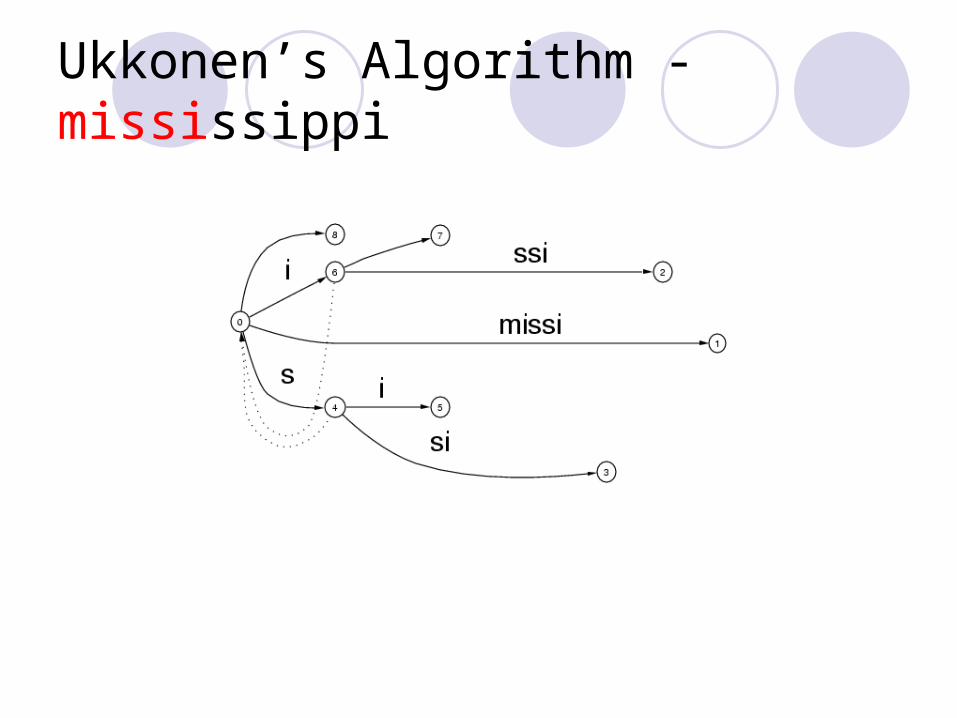
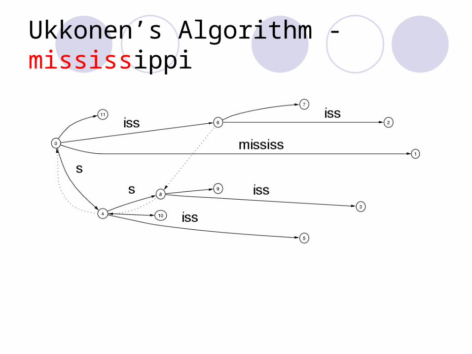
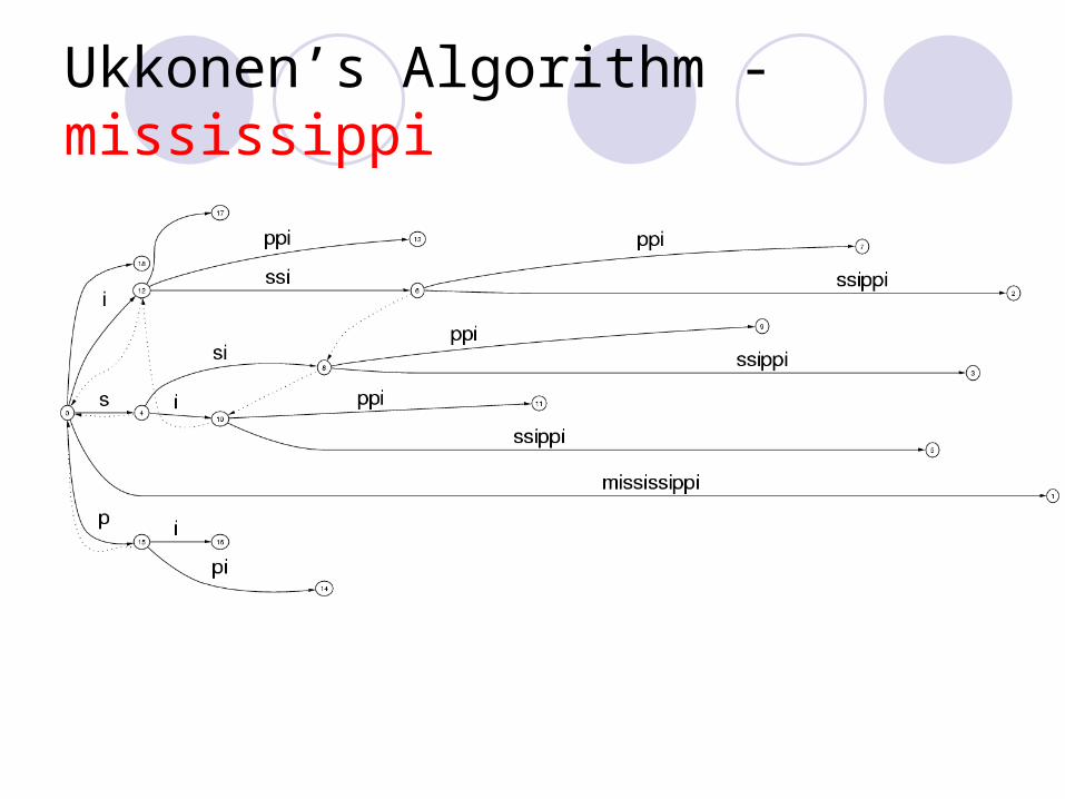
Ukkonen’s Algorithm
Build suffix tree T for string S[1..m] Build the tree in m phases, one for each
character. At the end of phase i, we will have tree Ti, which is the tree representing the prefix S[1..i].
In each phase i, we have i extensions, one for each character in the current prefix. At the end of extension j, we will have ensured that S[j..i] is in the tree Ti.
NTHU Make Lab http://make.cs.nthu.edu.tw

Ukkonen’s Algorithm
3 possible ways to extend S[j..i] with character i+1.
1. S[j..i] ends at a leaf. Add the character i+1 to the end of the leaf edge.
2. There is a path through S[j..i], but no match for the i+1 character. Split the edge and create a new node if necessary, then add a new leaf with character i+1.
3. There is already a path through S[j..i+1]. Do nothing.

Ukkonen’s Algorithm - mississippi

Ukkonen’s Algorithm - mississippi

Ukkonen’s Algorithm - mississippi

Ukkonen’s Algorithm - mississippi

Ukkonen’s Algorithm - mississippi
Ukkonen’s Algorithm - mississippi

Ukkonen’s Algorithm - mississippi
Ukkonen’s Algorithm - mississippi

Ukkonen’s Algorithm - mississippi

Ukkonen’s Algorithm - mississippi

Ukkonen’s Algorithm - mississippi
Ukkonen’s Algorithm - mississippi
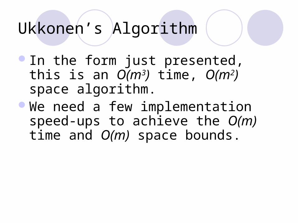
Ukkonen’s Algorithm
In the form just presented, this is an O(m3) time, O(m2) space algorithm.
We need a few implementation speed-ups to achieve the O(m) time and O(m) space bounds.
Suffix Array

The Suffix Array
Definition: Given a string D the suffixarray SA for this string is the sorted list of pointers toall suffixes of D.
(Manber, Myers 1990)

The Suffix Array In a suffix array, all suffixes of S are in the
non-decreasing lexical order. For example, S=“ATCACATCATCA”
3 ATCACATCATCA S(0)
10 TCACATCATCA S(1)
6 CACATCATCA S(2)
1 ACATCATCA S(3)
8 CATCATCA S(4)
4 ATCATCA S(5)
11 TCATCA S(6)
7 CATCA S(7)
2 ATCA S(8)
9 TCA S(9)
5 CA S(10)
0 A S(11)
i 0 1 2 3 4 5 6 7 8 9 10 11
A 11 3 8 0 5 10 2 7 4 9 1 6
0 A S(11)
1 ACATCATCA S(3)
2 ATCA S(8)
3 ATCACATCATCA S(0)
4 ATCATCA S(5)
5 CA S(10)
6 CACATCATCA S(2)
7 CATCA S(7)
8 CATCATCA S(4)
9 TCA S(9)
10 TCACATCATCA S(1)
11 TCATCA S(6)
中山大學資工系 --楊昌彪教授http://par.cse.nsysu.edu.tw/~cbyang/

fin

How do we build it ?
Build a suffix treeTraverse the tree in DFS, lexicographically
picking edges outgoing from each node and fill the suffix array.
O(n) timeSuffix tree construction loses some of the
advantage that the suffix array has over the suffix tree
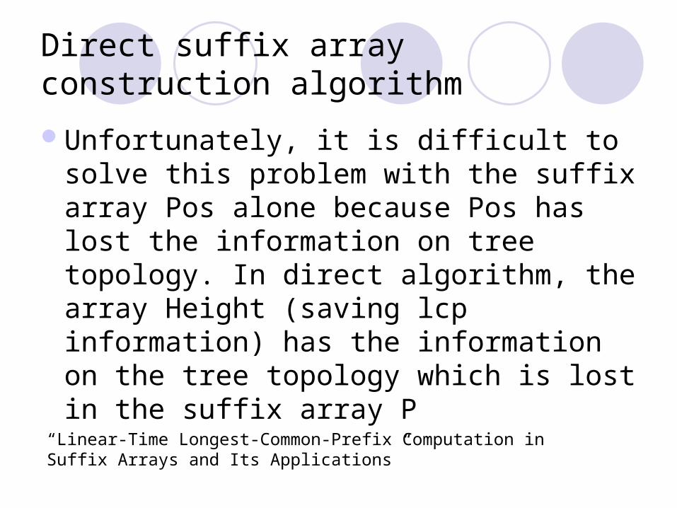
Direct suffix array construction algorithm
Unfortunately, it is difficult to solve this problem with the suffix array Pos alone because Pos has lost the information on tree topology. In direct algorithm, the array Height (saving lcp information) has the information on the tree topology which is lost in the suffix array P
“Linear-Time Longest-Common-Prefix Computation in Suffix Arrays and Its Applications”
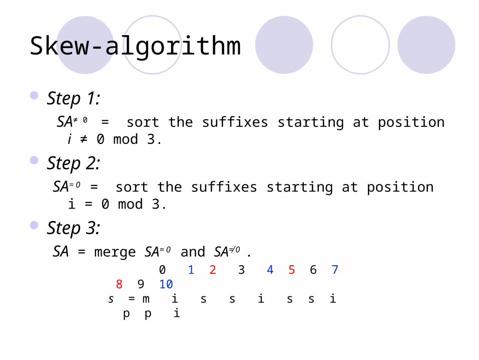
Skew-algorithm
Step 1: SA≠ 0 = sort the suffixes starting at position i ≠ 0 mod 3.
Step 2:SA= 0 = sort the suffixes starting at position i = 0 mod 3.
Step 3:SA = merge SA= 0 and SA≠ 0 .
0 1 2 3 4 5 6 7 8 9 10s = m i s s i s s i p p i

0 1 2 3 4 5 6 7 8 9 10
s = m i s s i s s i p p i
Radix sort
Step 1: SA≠ 0 = sort the suffixes starting at position i ≠ 0 mod 3.
3 3 2 1 5 5 4
Let S12 = [ 3 3 2 1 5 5 4 ]
1 4 7 10 2 5 8
=> SA≠0 = [ 10 7 4 1 8 5 2 ] in T(2n/3)
11 12
$ $ m i s s i s s i p p i
0 1 2 3 4 5 6 7 8 9 10

1 4 7 10 2 5 8
s12 = [ 3 3 2 1 5 5 4 ]
s121 = 3 3 2 1 5 5 4
s124 = 3 2 1 5 5 4
s127 = 2 1 5 5 4
s1210 = 1 5 5 4
s122 = 5 5 4
S125 = 5 4
s128 = 4
s = m i s s i s s i p p i
s1 = i s s i s s i p p i
s4 = i s s i p p i
s7 = i p p i
s10 = i
s2 = s s i s s i p p i
s5= s s i p p i
s8 = p p iSA≠ 0 = [ 10 7 4 1 8 5 2 ],
It suffices to show that S12i < S12
j <=> si < sj.

Compare Si and Sj where i = 0 , j ≠ 0 mod 3:
case 1: j = 1 mod 3
∵ i + 1 = 1 mod 3, j+1 = 2 mod 3
∴ compare (s[i], Si+1 ) with (s[j], Sj+1 )
in constant time.
case 2: j = 2 mod 3
∵ i + 2 = 2 mod 3, j+2 = 1 mod 3
∴ compare (s[i], s[i+1], Si+2) with
(s[j], s[j+1], Sj+2) in constant time

Case 1: i = j mod 3
1 4 7 10 2 5 8 0 1 2 3 4 5 6 7 8 9 10 11 12 s12 = [ 3 3 2 1 5 5 4 ] s = m i s s i s s i p p i $ $
Ex: 4 7 10 2 5 8 4 5 6 7 8 9 10 11 12s12
4 = [ 3 2 1 5 5 4 ] s4 = [ i s s i p p i $ $ ]
1 4 7 10 2 5 8 1 2 3 4 5 6 7 8 9 10 11 12s12
1 = [ 3 3 2 1 5 5 4 ] s1 = [ i s s i s s i p p i $ $ ]
S12i < S12
j <=> si < sj
s124 < s12
1s4 < s1

Case 2: i ≠ j mod 3 1 4 7 10 2 5 8 0 1 2 3 4 5 6 7 8 9 10 11 12s12 = [ 3 3 2 1 5 5 4 ] s = m i s s i s s i p p i $ $
Ex: 4 7 10 2 5 8 4 5 6 7 8 9 10 11 12s12
4 = [ 3 2 1 5 5 4 ] s4 = [ i s s i p p i $ $ ]
5 8 5 6 7 8 9 10 s12
5 = [ 5 4 ] s5 =[ s s i p p i ]
S12i < S12
j <=> si < sj
s124 < s12
5 s4 < s5

Step 2: SA= 0 = sort the suffixes starting at position i = 0 mod 3.
The rank of sj among {sk | k ≠ 0 mod 3 } was determined in Step1 for all j ≠ 0 mod 3.
SA=0 = radix sort { (s[i], Si+1 ) | i = 0 mod 3 }.
0: (m, ississippi)
3: (s, issippi)
6: (s, ippi)
9: (p, i)
0: (m, ississippi)
9: (p, i)
6: (s, ippi)
3: (s, issippi)
Radix sort
0 1 2 3 4 5 6 7 8 9 10s = m i s s i s s i p p i
(s[i], Si+1 )
9: (p, i)
6: (s, ippi)
3: (s, issippi)
0: (m, ississippi)
Step 1

Step 3: SA = merge SA= 0 and SA≠ 0 .
SA= 0 = [s0 s9 s6 s3]
SA≠0 = [s10 s7 s4 s1 s8 s5 s2]
SA = merge SA= 0 and SA≠0
=[s10 s7 s4 s1 s0 s9 s8 s6 s3 s5 s2]
= [10 7 4 1 0 9 8 6 3 5 2] It is in time O(n) if we can determine the relative
order of Si SA= 0 and Sj SA≠0 in constant
time.
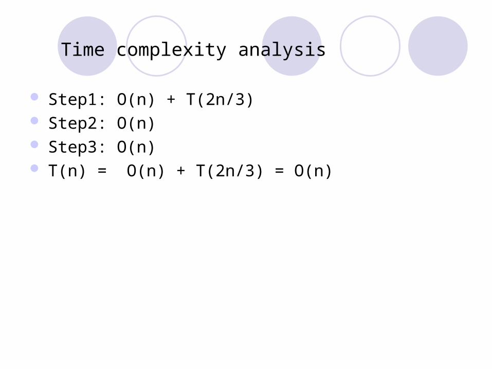
Time complexity analysis
Step1: O(n) + T(2n/3) Step2: O(n) Step3: O(n) T(n) = O(n) + T(2n/3) = O(n)

Exact matching using a Suffix Array
A B A A B B A B B A C
SA = 2 0 3 6 9 1 5 8 4 7 10
Basic Idea: 2 binary searches in SASearch for leftmost positionSearch for rightmost position
SUFFIX ARRAY SA:
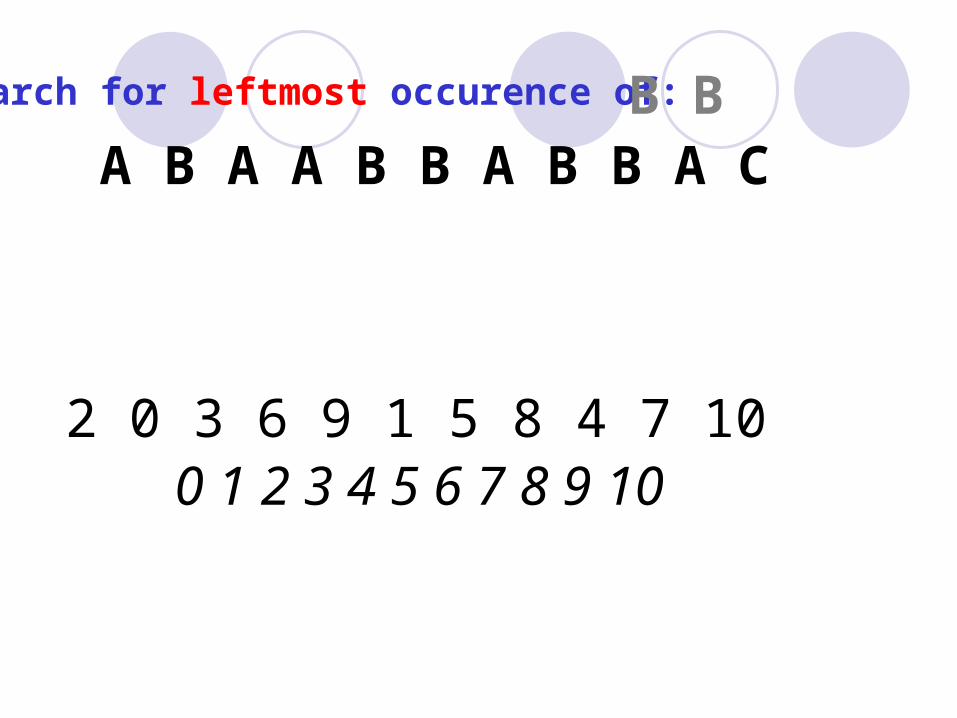
A B A A B B A B B A C
2 0 3 6 9 1 5 8 4 7 10
Search for leftmost occurence of: B B
0 1 2 3 4 5 6 7 8 9 10
Search for leftmost occurence of: B B
0 1 2 3 4 5 6 7 8 9 10
A B A A B B A B B A C
2 0 3 6 9 1 5 8 4 7 10
BB > BA
Continue binary search in the right (larger) half of SA

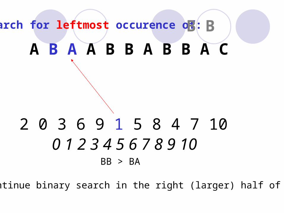
Search for leftmost occurence of: B B
0 1 2 3 4 5 6 7 8 9 10
A B A A B B A B B A C
2 0 3 6 9 1 5 8 4 7 10
BB = BB
More occurences of BB left of this one possible!

Search for leftmost occurence of: B B
0 1 2 3 4 5 6 7 8 9 10
A B A A B B A B B A C
2 0 3 6 9 1 5 8 4 7 10
BB > BA
leftmost position of BB is pointed to by SA[8]

Search for rightmost occurence of: B B
0 1 2 3 4 5 6 7 8 9 10
A B A A B B A B B A C
2 0 3 6 9 1 5 8 4 7 10
BB = BA
More occurences of BB right of this one possible!

Search for rightmost occurence of: B B
0 1 2 3 4 5 6 7 8 9 10
A B A A B B A B B A C
2 0 3 6 9 1 5 8 4 7 10
BB < C
rightmost position of BB is pointed to by SA[9]

Results of search for: B B
0 1 2 3 4 5 6 7 8 9 10
A B A A B B A B B A C
2 0 3 6 9 1 5 8 4 7 10
rightmost position of BB is pointed to by SA[9] leftmost position of BB is pointed to by SA[8]
=>All occurences of the pattern BB are pointed to by SA[8..9]

Important Properties
for |SA| = n and m = length of pattern:• Size : 1 Pointer per Letter (4 Byte if n < 4Gb)• Speed of exact matching :
• O(log n) binary search steps• # of compared chars is O(mlogn) can be reduced to O(m + log n)

Longest common prefixes
Definition: lcp(i,j) is the length of the longest common prefix of the suffixes beginning at SA[i] and SA[j].
Mississippi Example SA[2] = 4 (issippi) SA[3] = 1 (ississippi) lcp(2, 3) = 4
SA = [10 7 4 1 0 9 8 6 3 5 2]
s = m i s s i s s i p p i

Example
Let S = mississippiiippiissippiississippimississippipi
7
4
1
0
9
8
6
3
10
5
2
ppisippisisippissippississippi
L
R
Let P = issa
M
Haim Kaplan's home page
http://www.math.tau.ac.il/~haimk/
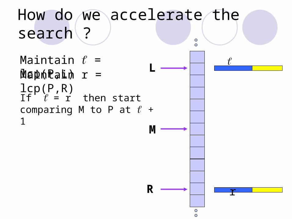
How do we accelerate the search ?
L
R
Maintain = lcp(P,L)Maintain r = lcp(P,R)
M
If = r then start comparing M to P at + 1
r

How do we accelerate the search ?
L
R
Suppose we know lcp(L,M)
If lcp(L,M) < we go left
If lcp(L,M) > we go right
If lcp(L,M) = we start comparing at + 1
M
If > r then
r
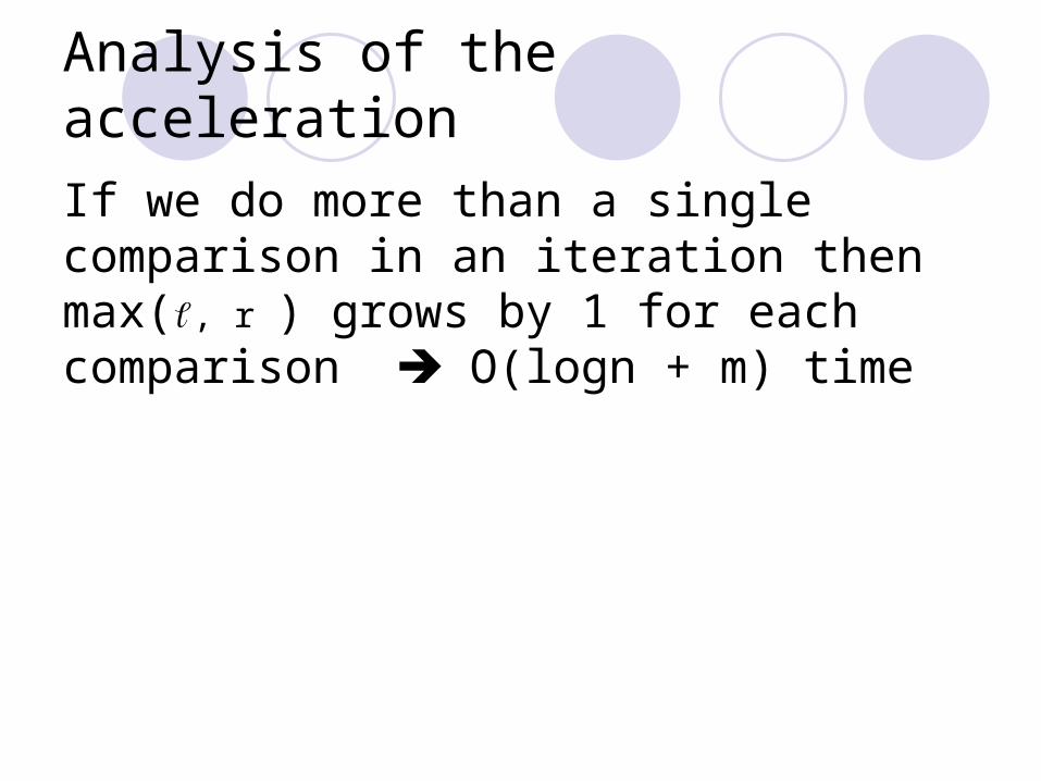
Analysis of the acceleration
If we do more than a single comparison in an iteration then max(, r ) grows by 1 for each comparison O(logn + m) time
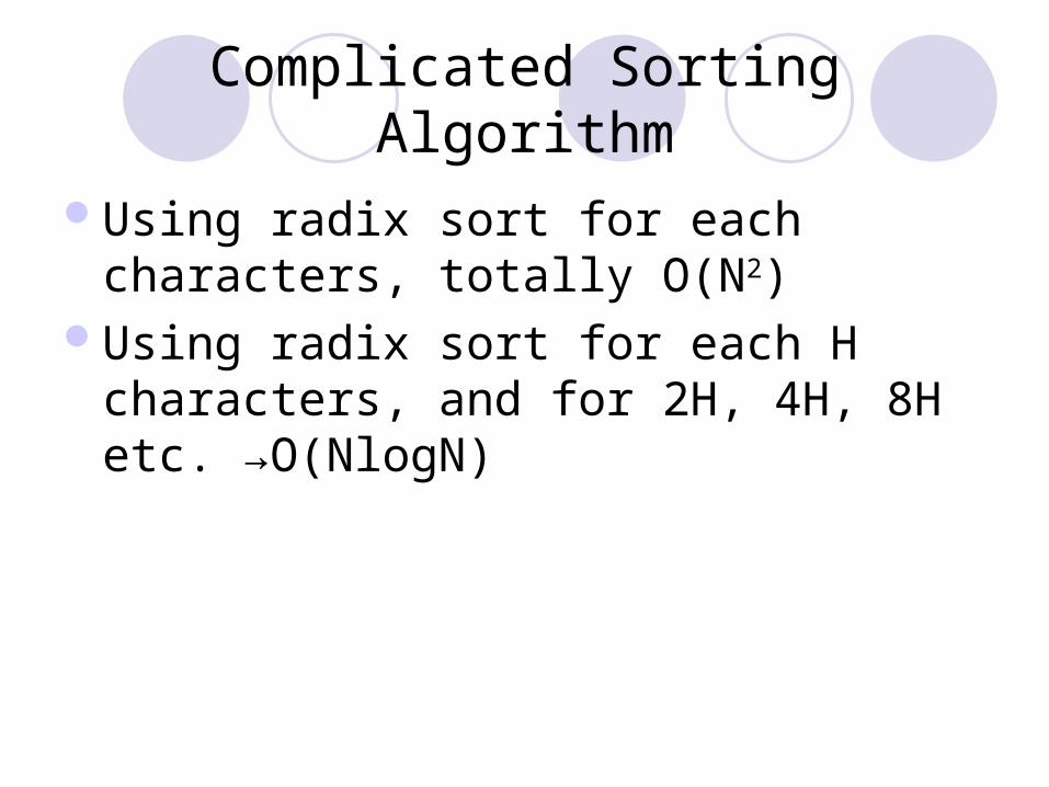
Complicated Sorting Algorithm
Using radix sort for each characters, totally O(N2)
Using radix sort for each H characters, and for 2H, 4H, 8H etc. →O(NlogN)
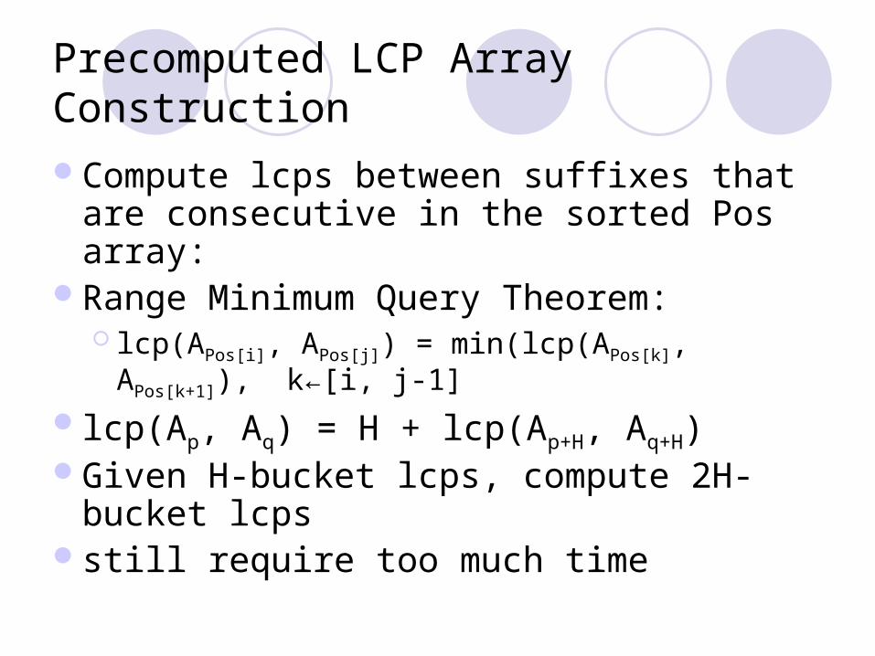
Precomputed LCP Array Construction
Compute lcps between suffixes that are consecutive in the sorted Pos array:
Range Minimum Query Theorem: lcp(APos[i], APos[j]) = min(lcp(APos[k], APos[k+1]), k←[i,
j-1]lcp(Ap, Aq) = H + lcp(Ap+H, Aq+H)Given H-bucket lcps, compute 2H-bucket
lcpsstill require too much time

Precomputed LCP Array Construction
Using height(i) = lcp(APos[i-1], APos[i])
Using Hgt[i] to record height(i) when it is correct
For b-th iteration if height(i) ≤ (b-1)H and height(i) < bH, then
Hgt[i] = height(i) Otherwise, Hgt[i] = N+1 (undefined)
Precomputed LCP Array Construction
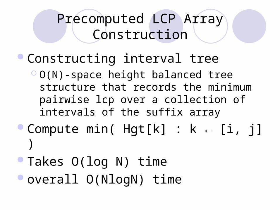
Constructing interval tree O(N)-space height balanced tree structure that
records the minimum pairwise lcp over a collection of intervals of the suffix array
Compute min( Hgt[k] : k ← [i, j] )Takes O(log N) timeoverall O(NlogN) time
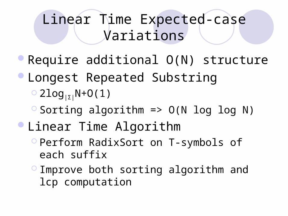
Linear Time Expected-case Variations
Require additional O(N) structureLongest Repeated Substring
2log|Σ|N+O(1) Sorting algorithm => O(N log log N)
Linear Time Algorithm Perform RadixSort on T-symbols of each suffix Improve both sorting algorithm and lcp
computation
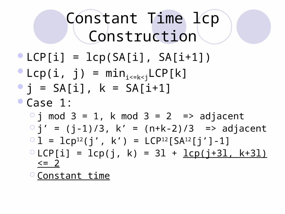
Constant Time lcp Construction
LCP[i] = lcp(SA[i], SA[i+1])Lcp(i, j) = mini<=k<jLCP[k]j = SA[i], k = SA[i+1]Case 1:
j mod 3 = 1, k mod 3 = 2 => adjacent j’ = (j-1)/3, k’ = (n+k-2)/3 => adjacent l = lcp12(j’, k’) = LCP12[SA12[j’]-1] LCP[i] = lcp(j, k) = 3l + lcp(j+3l, k+3l) <= 2 Constant time
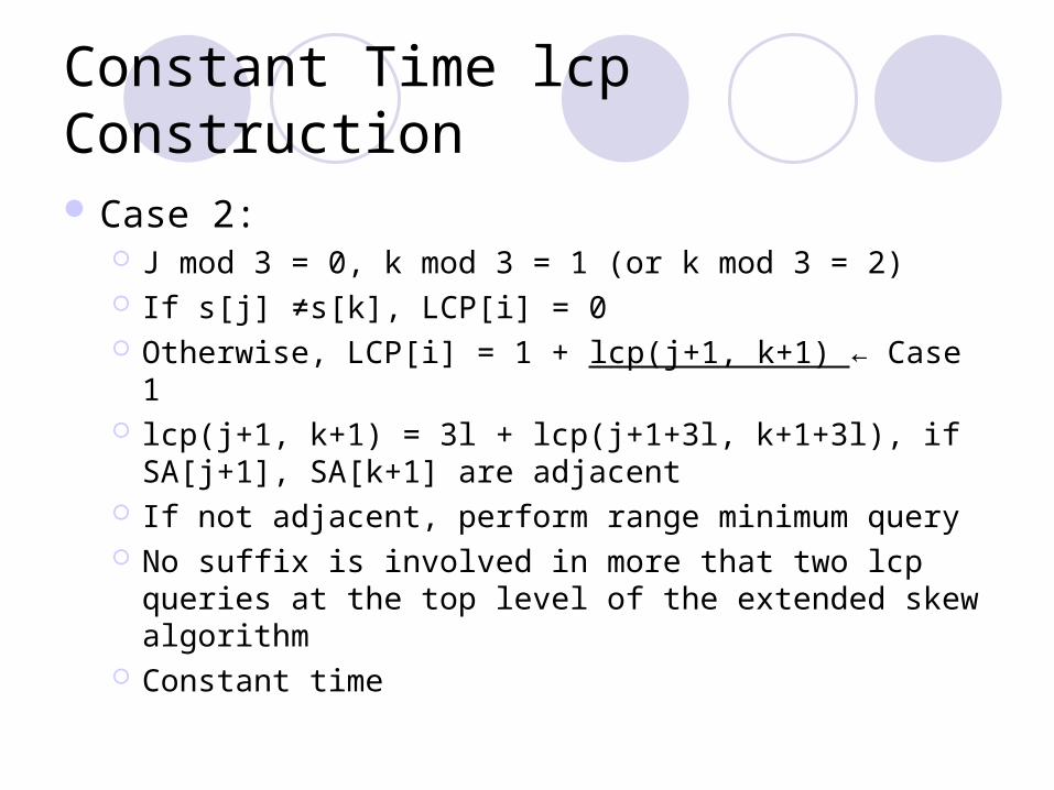
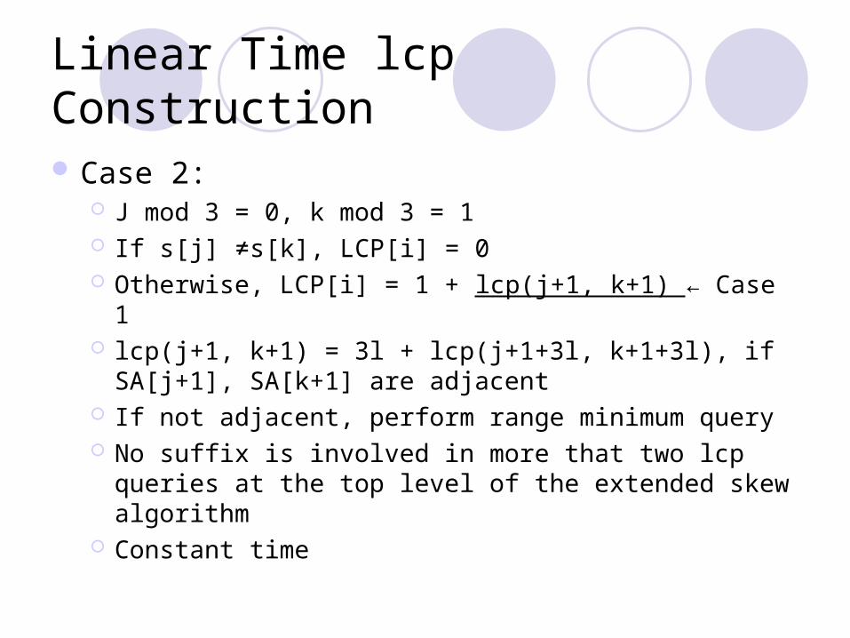
Constant Time lcp Construction
Case 2: J mod 3 = 0, k mod 3 = 1 (or k mod 3 = 2) If s[j] ≠s[k], LCP[i] = 0 Otherwise, LCP[i] = 1 + lcp(j+1, k+1) ← Case 1 lcp(j+1, k+1) = 3l + lcp(j+1+3l, k+1+3l), if SA[j+1],
SA[k+1] are adjacent If not adjacent, perform range minimum query No suffix is involved in more that two lcp queries at the
top level of the extended skew algorithm Constant time

Linear Time lcp Construction
LCP[i] = lcp(SA[i], SA[i+1])lcp(i, j) = mini<=k<jLCP[k]j = SA[i], k = SA[i+1]Case 1:
j mod 3 = 1, k mod 3 = 2 j’ = (j-1)/3, k’ = (n+k-2)/3 => adjacent in SA12
l = lcp12(j’, k’) = LCP12[SA12[j’]] LCP[i] = lcp(j, k) = 3l + lcp(j+3l, k+3l) <= 2 Constant time

Linear Time lcp Construction
LCP12 is used to decide triple-lcps ( groups of lcps of 3 characters )
0 1 2 3 4 5 6 7 8 9 0m i s s i s s i p p i
s12 = [ 3 3 2 1 5 5 4 ]
SA12 = [ 3 2 1 0 6 5 4 ]
LCP12 = [ 0 0 1 0 0 1 0 ]

Linear Time lcp Construction
To answer range minimum queries on LCP12 needs O(n) time
Lemma: No suffix is involved in more than two lcp queries at the top level of the extended skew algorithm A suffix can be involved in lcp queries only with
its two lexicographically nearest neighbors that have the same preceding character

Linear Time lcp Construction
LCP12 construction algorithm LCP12 array is divided into blocks of size log(n) For each block [a, b], precompute and store the following data:
For all i ← [a, b], Qi identifies all j ← [a, i] such that LCP12[j] < mink ←[j+1, i] LCP12[k]
For all i ← [a, b], the minimum values over the ranges [a, i] and [i, b] The minimum for all ranges that end just before or begin just after
[a, b] and contain exactly a power of two full blocks [i, j] is completely inside a block
Its minimum can be found with the help of Qj in constant time [i, j] is covered with some ranges whose minimun is stored
Its minimum is the smallest of those minima
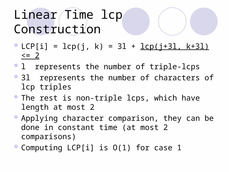
Linear Time lcp Construction
LCP[i] = lcp(j, k) = 3l + lcp(j+3l, k+3l) <= 2 l represents the number of triple-lcps 3l represents the number of characters of lcp
triples The rest is non-triple lcps, which have length at
most 2 Applying character comparison, they can be
done in constant time (at most 2 comparisons) Computing LCP[i] is O(1) for case 1
Linear Time lcp Construction
Case 2: J mod 3 = 0, k mod 3 = 1 If s[j] ≠s[k], LCP[i] = 0 Otherwise, LCP[i] = 1 + lcp(j+1, k+1) ← Case 1 lcp(j+1, k+1) = 3l + lcp(j+1+3l, k+1+3l), if SA[j+1],
SA[k+1] are adjacent If not adjacent, perform range minimum query No suffix is involved in more that two lcp queries at the
top level of the extended skew algorithm Constant time

Applications of Suffix Trees and Suffix Arrays
Exact String Match The Exact Set Matching Problem
The problem of finding all occurrences from a set of strings P in a text T, where the set is input all at once.
The Substring Problem for a Database of Patterns A set of strings, or a database, is first known and fixed.
Later sequence of strings will be presented and for each presented string S, the algorithm must find all the strings in the database containing S as a substring.
Applications of Suffix Trees and Suffix Arrays
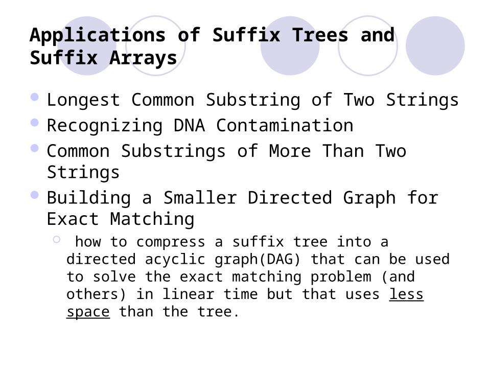
Longest Common Substring of Two Strings Recognizing DNA Contamination Common Substrings of More Than Two Strings Building a Smaller Directed Graph for Exact
Matching how to compress a suffix tree into a directed acyclic
graph(DAG) that can be used to solve the exact matching problem (and others) in linear time but that uses less space than the tree.
Applications of Suffix Trees and Suffix Arrays
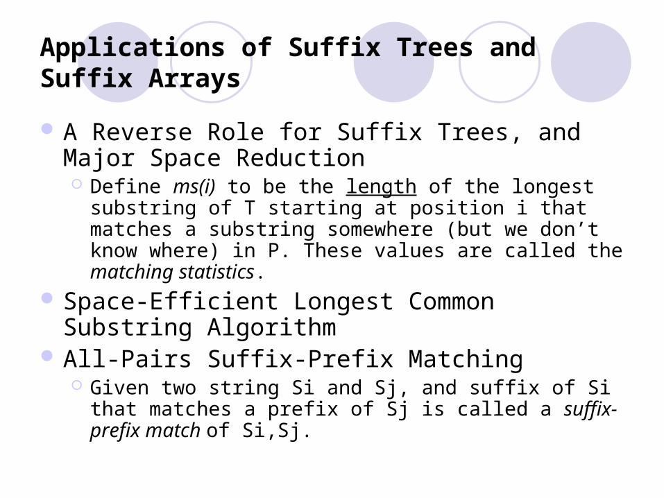
A Reverse Role for Suffix Trees, and Major Space Reduction Define ms(i) to be the length of the longest substring of
T starting at position i that matches a substring somewhere (but we don’t know where) in P. These values are called the matching statistics.
Space-Efficient Longest Common Substring Algorithm
All-Pairs Suffix-Prefix Matching Given two string Si and Sj, and suffix of Si that matches
a prefix of Sj is called a suffix-prefix match of Si,Sj.

Suffix Trees and Suffix Arrays
Suffix Each position in the text is considered as a text suffix.
A string that does from that text position to the end to the text
Advantage They answer efficiently more complex queries.
Drawback Costly construction process The text must be readily available at query time The results are not delivered in text position order.
NLP Laboratory of Hanshin University http://infocom.chonan.ac.kr/~limhs/
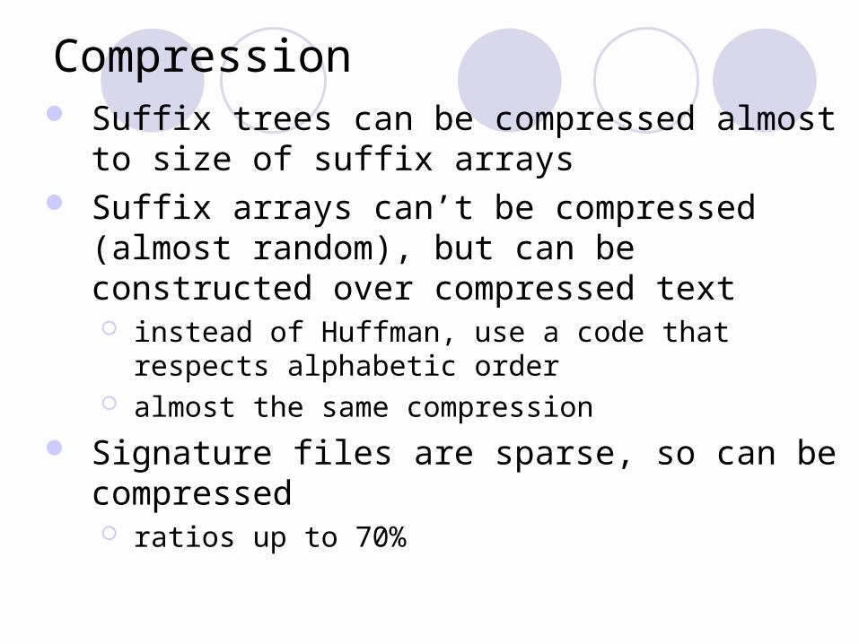
Compression Suffix trees can be compressed almost to size of
suffix arrays Suffix arrays can’t be compressed (almost
random), but can be constructed over compressed text instead of Huffman, use a code that respects
alphabetic order almost the same compression
Signature files are sparse, so can be compressed ratios up to 70%

Compression
Suffix trees and suffix arrays Suffix arrays are very hard to compress further.
Because they represent an almost perfectly random permutation of the pointers to the text.
Suffix arrays on compressed text The main advantage is that both index construction and
querying almost double their performance.• Construction is faster because more compressed text fits in the
same memory space and therefore fewer text blocks are needed.
• Searching is faster because a large part of the search time is spent in disk seek operations over the text area to compare suffixes.
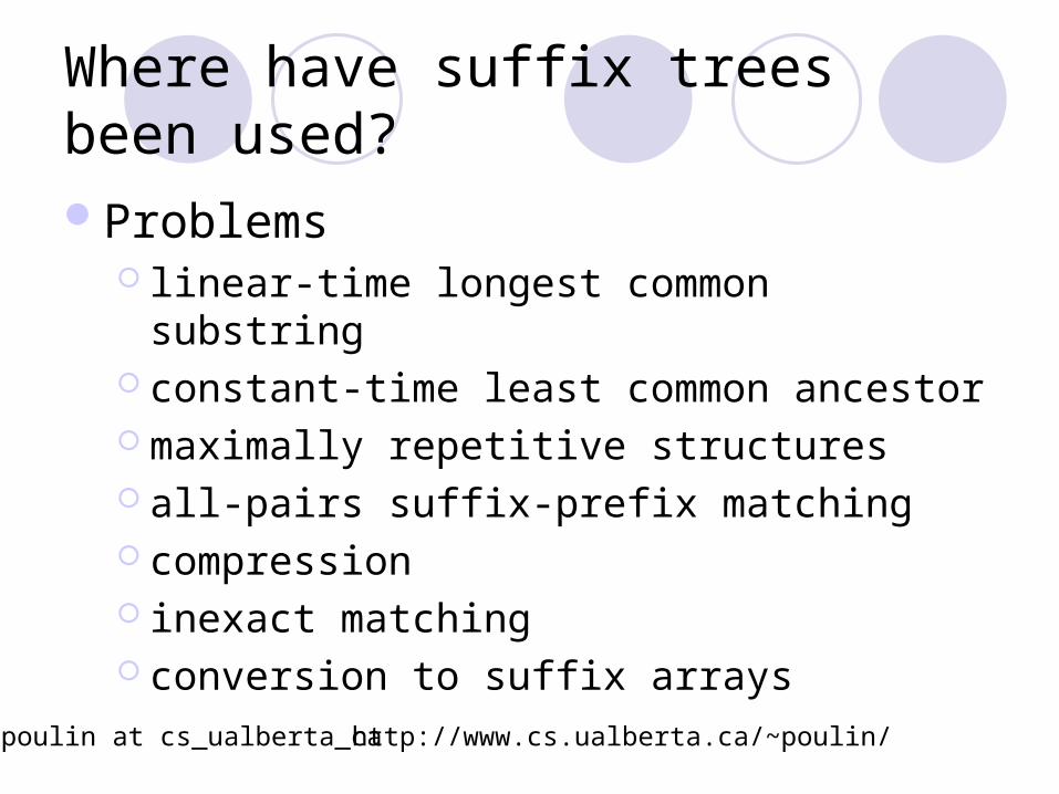
Where have suffix trees been used?
Problems linear-time longest common substring constant-time least common ancestor maximally repetitive structures all-pairs suffix-prefix matching compression inexact matching conversion to suffix arrays
poulin at cs_ualberta_ca http://www.cs.ualberta.ca/~poulin/

Where have suffix trees / arrays been used?
Applications The Human Genome Project (see Skiena) motif discovery (see Arabidopsis genome
project) PST – probabilistic suffix trees SVM string kernels chromosome-level similarities and
rearrangements

When have suffix trees / arrays been used?
When they solve your problem.When you need results fast!When you have memory to spare.…more caveats.

fin