suitability of numerical modelling approach of an …
TRANSCRIPT

SUITABILITY OF NUMERICAL MODELLING APPROACH
OF AN INTEGRAL BRIDGE FOR STRENGTHENING OF
RC PILE FOUNDATION USING SSI
A Thesis Submitted
in Partial Fulfilment of Requirements
for the Degree of
DOCTOR OF PHILOSOPHY
by
Sreya Dhar
DEPARTMENT OF CIVIL ENGINEERING
INDIAN INSTITUTE OF TECHNOLOGY GUWAHATI
GUWAHATI-781039, INDIA
June 2018
TH-2208_126104008

To my grandparents and loving sister..
TH-2208_126104008

TH-2208_126104008

Abstract
Integral Abutment Bridges (IABs) have become widely popular in the recent years due
to the absence of bearings at the junction of bridge deck and bridge abutment. That
leads to a reduction in the overall maintenance cost of the bridge. However, the
monolithic action of deck-abutment junction changes the behaviour of the overall bridge
under temperature loading and earthquake shaking. In an integral abutment bridge,
bearings may be absent at the locations of the piers also. Then, the bridge is known as a
fully integral bridge. In such a bridge, the behaviour of the bridge tends to follow frame-
type action with all the junctions of the deck and the vertical members acting as
monolithic units. Although, past studies have been carried out on behaviour under
temperature variation for both the types of bridges, detailed investigations of seismic
behaviour of the bridge with different modelling approaches of soil-structure
interaction, have not been carried out. Also, the pile foundations below bridges have
been observed to undergo failure during past earthquakes and this necessitates further
investigations. All these provide the motivation for the current study.
In the present study, a multi-span RC integral bridge on RC pile foundation is
first modelled using an open source program, OpenSees, with stratified foundation soil.
For modelling Soil-Structure Interaction (SSI), two approaches are implemented
separately, namely (a) soil domain approach in which the soil is modelled as a
continuum, and (b) spring-dashpot approach in which the lateral strength and stiffness
of the soil are modelled considering Beam on Dynamic Winkler Foundation concept.
Based on the site details (the real bridge site is located in California, USA, from which
the bridge characteristics have been taken), seven ground motions are selected from a
strong ground motion database by matching of mean displacement spectrum for all the
ground motions with a target spectrum. Under the selected site-specific ground motions,
TH-2208_126104008

���������
______________________________________________________________________
ii
nonlinear time history analyses are carried out for different models with changes in
boundary conditions at the bottom of the piers, presence or absence of backfill soil and
the two different SSI modelling approaches. The variations in the deformation at bridge
deck level and section level response of the piers are observed. As compared to the soil
domain approach, the spring-dashpot approach is observed to provide conservative
estimates of forces and moments, and possibly can be recommended for implementation
in seismic design.
For an integral bridge, the overall length of the bridge tends to play a major role
in the response under temperature loading. The same parameter is expected to
significantly influence the overall bridge response during earthquake shaking. In the
second part of the study, the overall length of the same integral bridge is changed and
nonlinear time history analysis is carried out under site specific ground motions using
the spring-dashpot model for different types of foundation soil. With increase in overall
length, inelasticity is observed in the response of pier and pile foundation for certain
soils. Consequently, one of the retrofitting methods for pile foundation, i.e., through
installation of new piles encased in jet grout, is implemented on the pile groups below
abutments and the piers in two separate stages. The numerical modelling of the
encasement method is carried out using suitable spring-dashpots to model the soil and
the grout around the new piles. For certain soils, the response of the bridge gets
significantly improved through reduction of nonlinear behaviour of the components,
after applying the retrofitting method.
In a summary, the present thesis tends to provide insight into the seismic
behaviour of an integral bridge with RC pile foundation from the aspects of different
numerical modelling approaches, influence of overall length and improvement in the
response of pile foundation through encasement method of retrofitting.
TH-2208_126104008

Acknowledgement
Part of this research was carried out while the author of thesis (S. Dhar) was visiting
Politecnico di Milano (PoliMi) Italy, under INTERWEAVE Project, Erasmus Mundus
Program during 2014-2017. The author would like to thank Ministry of Human
Resources (MHRD) for the scholarship during PhD work.
I express my sincere gratitude to my advisors Prof. Kaustubh Dasgupta and
Prof. Roberto Paolucci for their enthusiastic guidance, continued support and
encouragement throughout the course of the dissertation. I want to thank Prof. Lorenza
Petrini for her immense help during my thesis work. Her motivations and many fruitful
discussions are greatly appreciated. I have learnt many things from my mentor Dr. Ali
Günay Özcebe, post-doctoral scholar in PoliMi, in academic and non-academic aspects,
which I will try to reflect in my future career. I want to thank my doctoral committee
members, Prof. Sudip Talukdar, Prof. Hemant B. Kaushik and Prof. Pankaj Biswas for
their fruitful comments on my thesis.
I am deeply indebted to my grandparents for their love and affection from my
childhood. I want to thank my motherly sister who have guided me in thick and thin. I
dedicate my thesis to all of them . . .
My deepest thanks go to my parents, for their warm support and unparalleled
affection. I want to thank my husband Swarnava and my parents in law for their
immense support. My personal gratitude and respects to Prof. Hemant B. Kaushik, Dr.
Snehal and Benazir for their warm support and care.
I thank Dr. Geetimukta for her help during my PhD. I also thank Sophia, Dr.
Isha, Anjaly, Thianswemong for their warm friendship.
TH-2208_126104008

TH-2208_126104008
______________________________________________________________________
Table of Contents Abstract…………………………………………………………………………………..i
Acknowledgement……………………………………………………………………… iii
Table of Contents…………………………………………..…………………………….v
List of Figures…………………………..………………………………………………ix
List of Tables…………………………..…………………………….………..………xvii
List of Symbols………………………..…………………………….……….…..….…xix
Chapter 1 Introduction………………………………………………………………...1
1.1 Introduction ................................................................................................................ 1�
1.2 Seismic Soil Structure Interaction .............................................................................. 3�
1.3 Major Concern and the Motivation of the Study ........................................................ 4�
1.4 Objectives of the Study .............................................................................................. 5�
1.5 Outline of the Thesis .................................................................................................. 6
Chapter 2 Literature Review…………………………………………………………..9
2.1 Introduction ................................................................................................................ 9�
2.2 Characteristics of IAB ................................................................................................ 9�
2.2.1 Length .................................................................................................................. 9
2.2.2 Skew angle…………………………………………………….……………….10
2.2.3 Loadings on IAB ............................................................................................... 11�
2.3 Abutment Behaviour ................................................................................................ 13�
2.3.1 Foundation type ................................................................................................. 14�
2.3.2 Abutment backfill interaction ............................................................................ 17�
2.4 Soil Pile Interaction .................................................................................................. 22�
2.4.1 Computational approach .................................................................................... 26�
2.5 Field Studies ............................................................................................................. 29�
2.6 Code Provisions ........................................................................................................ 32�
TH-2208_126104008

�������
______________________________________________________________________
vi
2.7 Retrofitting of Pile Foundation ................................................................................. 33�
2.8 Summary ................................................................................................................... 35�
2.9 Gap Areas ................................................................................................................. 37�
2.10 Scope of Present Work ........................................................................................... 38�
Chapter 3 Modelling…………………………………………………………………..39
3.1 Introduction .............................................................................................................. 39�
3.2 Modelling ................................................................................................................. 40�
3.2.1 Modelling of bridge structure ............................................................................ 40�
3.2.2 Modelling of soil and foundation ...................................................................... 43�
3.2.3 Modelling of spring-dashpot system ................................................................. 45
Chapter 4 Site Resposne Analysis and Selection of Ground Motions……………..51
4.1 Introduction .............................................................................................................. 51�
4.2. Site Response Analysis (SRA) ................................................................................ 51�
4.3 Selection of Ground Motions ................................................................................... 55�
Chapter 5 Seismic Analysis of RC Integral Bridge………...………………..……...59
5.1 Introduction .............................................................................................................. 59�
5.2 Analysis .................................................................................................................... 59�
5.3 Linear and Nonlinear Time History Analyses .......................................................... 61�
5.3.1. Structural response ........................................................................................... 62�
5.3.1.1 Response of pier sections ........................................................................... 68�
5.3.2 Response of soil ................................................................................................. 69�
5.3.3 Response of full SSI no BA model across depth ................................................ 75�
5.4 Complementary Investigation of Material Properties in Full SSI No BA Model ..... 77�
5.4.1 Linear structural behaviour ................................................................................ 78�
5.4.2 Nonlinear structural behaviour .......................................................................... 80�
5.5 Influence of Abutment Backfill Interaction.............................................................. 82�
5.6 Introduction of Nonlinear Spring-Dashpot Model ................................................... 89�
TH-2208_126104008

�������
______________________________________________________________________
vii
5.6.1 Comparison between full SSI no BA and FB_SD no BA models ....................... 89�
5.6.2 Comparison between full SSI with BA and FB_SD with BA models .............. 92�
5.7 Mean Maximum Response ....................................................................................... 96�
5.8 Discussion ................................................................................................................. 99
Chapter 6 Study on Overall Length of Integral Bridge……………………..…….103
6.1 Introduction ............................................................................................................ 103�
6.2 Modelling ............................................................................................................... 104�
6.2.1 Structure and Foundation Properties ............................................................... 104�
6.2.2 Properties of Soil links .................................................................................... 105�
6.3 Analysis .................................................................................................................. 108�
6.4 Results .................................................................................................................... 110�
6.4.1 Response for medium stiff clay soil ................................................................ 110�
6.4.2 Response for loose sand .................................................................................. 113�
6.4.3 Comparison of response in loose sand and medium clay soil ......................... 115�
6.4.4 Response of bridge in dense sand and soft clay .............................................. 118�
6.5 Summary ................................................................................................................. 119
Chapter 7 Retrofitting of Pile Foundation…...…………………………………….121
7.1 Introduction ............................................................................................................ 121�
7.2 Retrofitting of RC Pile Foundation ........................................................................ 122�
7.2.1 Modelling of encasement method.................................................................... 122�
7.2.2 Encasement method at pier pile foundation .................................................... 124�
7.3 Analysis .................................................................................................................. 125�
7.4 Results .................................................................................................................... 126�
7.4.1 Comparison between M1 and M2 models ....................................................... 126�
7.4.2 Comparison between M2 and M3 models ....................................................... 131�
7.5 Discussion ............................................................................................................... 135
Chapter 8 Conclusions and Future Scope of Work……………..…………………137
TH-2208_126104008

Contents
viii
8.1 Conclusions ............................................................................................................ 137
8.2 New Contributions of the Present Study ................................................................ 139
8.3 Scope of Future Work ............................................................................................ 140
References……………………………………………………………...……………..141
Appendix A .................................................................................................................. 151
Appendix B ................................................................................................................... 152
Appendix C ................................................................................................................... 154
Appendix D .................................................................................................................. 156
Appendix E ................................................................................................................... 158
Appendix F ................................................................................................................... 159
Appendix G .................................................................................................................. 160
TH-2208_126104008

______________________________________________________________________
List of Figures
Fig. 1.1 A typical single span jointless bridge .................................................................. 1�
Fig. 1.2 Fully integral abutment bridge (Yannotii et al., 2005) ....................................... 2�
Fig. 1.3 Semi-integral abutment bridge (Yannotti et al., 2005) ....................................... 3�
Fig. 1.4 Deck extension abutment (Yannotti et al., 2005)................................................ 3�
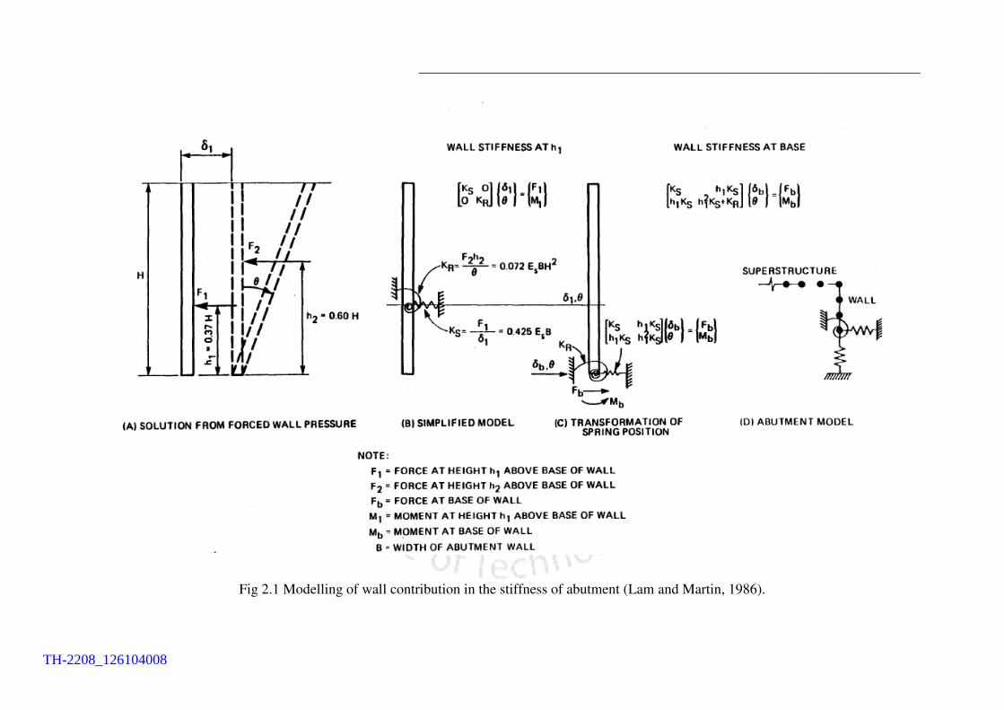
Fig 2.1 Modelling of wall contribution in the stiffness of abutment (Lam and Martin,
1986). ...................................................................................................................... 16�
Fig. 2.2 Comparison of design curves given in different manual (Faraji et al., 1998) ... 18�
Fig. 2.3 Hyperbolic force-displacement formulation for abutment-backfill interaction
(Shamsabadi et al., 2007). ...................................................................................... 19�
Fig. 2.4 Earth pressure distributions on framed abutments (BA 42/96, 2003) ............... 20�
Fig. 2.5 Variation of passive earth pressure with the lateral displacement of abutment wall
(Claugh and Duncan, 1991) .................................................................................... 21�
Fig. 2.6 General schematic of the finite element (FE) model used for the BNWF analyses
using the nonlinear fiber beam-column element and the nonlinear p-y element
(Hutchinson et al., 2004). ....................................................................................... 25�
Fig. 2.7 (a) Proposed discrete lumped mass with spring-dashpot model (Khodabhakhshi
et al., 2011) and (b) generic soil-structure foundation system. .............................. 26�
Fig.2.8 (a) Lysmer Viscous Boundary and (b) Consistent Boundary ............................ 28�
Fig 2.9 Schematic of Pile-to-Cap Hinged Connection ................................................... 30�
Fig. 2.10 Schematic of jet-grouting reinforced pile (He et al., 2016); where, hg = height
of jet grout, dp = diameter of pile and dg = diameter of grout. ............................... 35�
Fig: 3.1(a) Backbone curve of Concrete01 material for core and cover, (b) backbone curve
of Steel02 material in tension for reinforcement and (c) Locations of monitored fiber
locations in a pier cross section (all dimensions are in m). .................................... 42�
Fig. 3.2 (a) Modified 1D Soil column with soil classification (Zhang et al., 2008), (b)
variation of shear modulus with shear strain for different soil layers, (c) variation of
damping ratio with shear strain for different soil layers (Darendeli, 2001) and (d)
complete soil-foundation-bridge model with abutment backfill (all dimensions are
in m) ........................................................................................................................ 44�
Fig. 3.3 Schematic diagram of (a) soil-pile interaction , (b) abutment-backfill interaction
and (c) Rayleigh damping considered for analysis (For the notations refer to Table
5.1). ......................................................................................................................... 47�
TH-2208_126104008

��������������
______________________________________________________________________
x
Fig. 3.4 Variation of (a) lateral force with lateral displacement for Pile_2, (b) skin friction
with vertical displacement at the depth of 5.2 m, (c) pile tip end bearing load with
vertical displacement at the depth of 5.2 m and (d) the lateral force with lateral
displacemnt at abutment-backfill interface for different depths. ............................ 48�
Fig. 4.1 (a) Nested plasticity theory and (b) octahedral shear stress–strain curve in
OpenSees (McKenna, 2008), (c) a typical loading-unloading behaviour for material
of Masing type (Rocha and Lopez, 2008). ............................................................. 53�
Fig. 4.2 Linear soil column analyses: (a) horizontal acceleration time history (HATHs) of
soil column at surface, (b) HATHs of soil column at 5 m from the base, profiles of
(c) maximum horizontal acceleration and (d) maximum shear strain along the depth
of column. ............................................................................................................... 54�
Fig. 4.3 Nonlinear soil column analyses: (a) HATHs of soil column at surface, (b)
HATHS of soil column at 5 m from the base, profiles of (c) maximum horizontal
acceleration and (d) maximum shear strain along the depth of column. ................ 54�
Fig. 4.4 Displacement spectra of all the ground motions used in present study ............ 56�
Fig. 4.5 Velocity time histories of all the seven ground motions used in the present study.
................................................................................................................................ 57�
Fig. 5.1 Schematic diagram of only B_FF/SSI model in OpenSees ............................... 60�
Fig. 5.2 Details of full SSI no BA model in OpenSees: (a) overall schematic diagram and
(b) locations in soil domain for monitoring response (all dimensions are in m). ... 61�
Fig. 5.3 Rock outcrop earthquake (scaled) ground motions (a) GM#1 and (b) GM#2;
Fourier amplitudes of (c) GM#1 and (d) GM#2 with fundamental frequencies
(marked) for the different models. .......................................................................... 62�
Fig. 5.4 SFTHs in LTHA (a) under GM#1, (b) under GM#2 and normalized Fourier
transform of SFTHs for (c) GM#1 and (d) GM#2.................................................. 64�
Fig. 5.5 Velocity time histories (VTHs) in LTHA at the top of 8th pier from LTHA (a)
under GM#1 and (b) under GM#2; Fourier amplitude of VTHs (c) under GM#1 and
(d) under GM#2. ..................................................................................................... 65�
Fig. 5.6 SFTHs under from NTHA under (a) GM#1 (b) GM#2, normalized FTs of SFTH
for (c) GM#1 and (d) GM#2. .................................................................................. 66�
Fig. 5.7 Velocity time histories (VTHs) in NTHA at the top of 8th pier from NTHA under
(a) GM#1 and (b) GM#2; Fourier amplitude of VTHs under (c) GM#1 and (d)
GM#2. ..................................................................................................................... 68�
Fig. 5.8 Average spectral acceleration at the base of only bridge models under GM#1. 68�
TH-2208_126104008

��������������
______________________________________________________________________
xi
Fig. 5.9 Stress-strain response of fibers under GM#1 at top cross section of 8th pier: for
(a) Steel fiber 1, (b) Steel fiber 2, (c) Core Concrete fiber 1, (d) Core Concrete fiber
2 (e) Cover concrete fiber 1 and (f) Cover concrete fiber 2 for full SSI no BA model
................................................................................................................................ 70�
Fig. 5.10 Moment-curvature response at top cross section of 8th pier (a) under GM#1, (b)
under GM#2, at base cross section of 1st pier (c) under GM#1 and (d) under GM#2
for full SSI no BA model ......................................................................................... 71�
Fig. 5.11 Variation of shear stress with shear strain in full SSI no BA model at Location#1,
due to (a) GM#1, (b) GM#2, at Location#2 due to (c) GM#1 and (d) GM#2........ 71�
Fig. 5.12 (a) Undeformed shape of full SSI no BA model and (b) deformed shape of full
SSI no BA model after dynamic analysis under GM#1 [image amplification factor is
100]. ........................................................................................................................ 72�
Fig. 5.13 Comparison of horizontal DTHs in soil domain at (a) different locations below
the bridge and (b) near the boundaries in free field soil domain and full SSI no BA
models under GM#1 (‘pg’ stands for pile group). .................................................. 73�
Fig. 5.14 Maximum horizontal acceleration profile along the depth of monitored soil
column under (a) GM#1 and (b) GM#2; maximum shear strain profile along the
depth of monitored soil column under (c) GM#1 and (d) GM#2. .......................... 76�
Fig. 5.15 Recorded ATHs along the vertical profile of right abutment-pile group-
foundation (a) under GM#1, (b) under GM#2; FTs of ATHs (c) under GM#1 and (d)
under GM#2 in full SSI no BA model. .................................................................... 77�
Fig.5.16 Comparison of SFTHs at the top of 8th pier of bridge for linear behaviour of full
SSI no BA model and lin str+nl soil no BA model under (a) GM# 1, (b) GM#2 and
normalized FTs of (c) SFTHs shown in (a) and (d) SFTHs shown in (b). ............. 79�
Fig. 5.17 Comparison of VTHs for linear behaviour of full SSI no BA model and lin str+nl
soil no BA model at the 8th pier top under (a) GM#1and (b) GM#2; normalised FTs
of VTHs under (c) GM#1 and (d) GM#2. .............................................................. 80�
Fig. 5.18 Comparison of SFTHs for the nonlinear behaviour of full SSI no BA model and
the nl str+lin soil no BA model at the top of 8th pier of bridge under (a) GM# 1 and
(b) GM#2; normalized FTs of SFTHs under (c) GM#1and (d) GM#2. ................ 82�
Fig.5.19 Comparison of VTHs at right abutment deck joint for the nonlinear behaviour
of full SSI no BA model and the nl str+lin soil no BA model under (a) GM#1 and (b)
GM#2; Fourier amplitudes of VTHs under (c) GM#1 and (d) GM#2. .................. 83�
TH-2208_126104008

��������������
______________________________________________________________________
xii
Fig. 5.20 (a) Undeformed shape and (b) deformed shape of full SSI with BA model after
dynamic analysis under GM#1. .............................................................................. 84�
Fig. 5.21 Comparison of (a) SFTHs at the top of 8th pier, (b) normalized FTs of SFTHs
shown in (a), (c) DTHs of soil node in pile-foundation below the 8th pier, and (d)
ATHs at the top of 8th pier under GM#1 for full SSI no BA model and full SSI with
BA model. ............................................................................................................... 86�
Fig. 5.22 Comparison of (a) SFTHs at the top of 8th pier, (b) normalized FTs of SFTHs
shown in (a) in log-log scale, (c) ATHs at 1st pier top, (d) FTs of ATHs shown in (c)
under GM#2 for full SSI no BA model and full SSI with BA model. ...................... 87�
Fig. 5.23 Comparison of moment curvature response at the (a) bottom and (b) top cross-
sections of the 8th pier under GM#1 for full SSI no BA model and full SSI with BA
model. ..................................................................................................................... 87�
Fig. 5.24 Stress-strain response at top of 8th pier cross-section for (a) Steel fiber 1, (b)
Steel fiber 2, (c) Core concrete fiber 3 and (d) Cover concrete fiber 3 shown in
Fig.3.1(a), under GM#1 for full SSI no BA and full SSI with BA models. .............. 88�
Fig. 5.25 Comparison of ATHs for full SSI no BA model and FB_SD no BA model under
GM#1 at (a) the bottom and (b) the top of the 8th pier; (c) FT of the ATHs shown in
(a) and (d) FT of the ATHs in (b). .......................................................................... 90�
Fig. 5.26 Comparison of (a) Shear Force time history at the top of 8th pier and (b)
normalised FTs of the SFTHs for the full SSI no BA model and FB_SD no BA model;
moment-curvature response at the (c) top and (d) bottom cross-sections of the of 8th
pier under GM#1. ................................................................................................... 91�
Fig. 5.27 (a) SFTH at the top of 8th pier and (b) normalised FTs of the SFTHs in (a) under
GM#2. ..................................................................................................................... 92�
Fig. 5.28 Comparison of ATHs for full SSI with BA model and FB_SD with BA model at
the (a) top and the (b) bottom of 8th pier; (c) Fourier transform of the ATHs shown
at the (a) bottom and (d) the top of 8th pier under GM#1. ...................................... 93�
Fig. 5.29 Comparison of ATHs for full SSI with BA model and FB_SD with BA model at
the (a) top and the (b) bottom of the 8th pier; Fourier transform of the ATHs shown
at the (c) bottom and the (d) top of the pier under GM#2 ...................................... 94�
Fig. 5.30 Comparison of SFTHs for full SSI with BA model and FB_SD with BA model
(a) at the top of the 8th pier and (b) normalised FTs of the SFTHs in (a) under GM#1;
(c) SFTHs at the top of 8th pier and (d) normalised FTs of the SFTHs in (c) under
GM#2 [FT plots in log-log scale] ........................................................................... 95�
TH-2208_126104008

��������������
______________________________________________________________________
xiii
Fig. 6.1 3D bridge model in SAP2000 founded on medium stiff clay ......................... 104�
Fig. 6.2 Reinforcement detailing of cross-sections for (a) pier, (b) pier piles and (c)
abutment piles. ...................................................................................................... 105�
Fig. 6.3 (a) Soil-pile interaction and (b) abutment-backfill interaction in medium stiff clay
.............................................................................................................................. 106�
Fig. 6.4 Comparison of backbone curves for loose sand and dense sand at the depths of
(a) 2 m and (b) 4 m, for soft clay and stiff clay at the depths of (c) 2 m and (d) 4 m
in case of intermediate pier piles. ........................................................................ 107�
Fig. 6.5 Comparison of backbone curves for loose sand and dense sand at the depths of
(a) 2 m and (b) 4 m, and for soft clay and stiff clay at the depths of (c) 2 m and (d) 4
m for abutment piles. ............................................................................................ 107�
Fig. 6.6 Models of bridges with (a) 7 spans, (b) 5 spans and (c) 3 spans. .................... 109�
Fig. 6.7 (a) Displacement spectra for all the GMs, (b) acceleration time history of GM#1,
(c) acceleration time history of GM#2 chosen for parametric study, (d) Fourier
amplitude of GM#1 and (e) Fourier amplitude of GM#2 [notations S9, S7, S5, S3
stand for 9span, 7span, 5span and 3span bridges natural frequencies]. ............... 109�
Fig. 6.8 Shear force response at the top of 3rd pier under (a) GM#1 and (b) GM#2;
moment-rotation response at the top of 3rd pier under (c) GM#1 and (d) GM#2 in
medium stiff clay soil. .......................................................................................... 111�
Fig. 6.9 Displacement time histories (DTHs) for bridges of 9span, 7span and 5span at (a)
top of abutment and (b) bottom of abutment under GM#1, (c) DTHs of 9span bridge
under GM#2 in medium stiff clay foundation soil. .............................................. 112�
Fig. 6.10 Moment-rotation response of abutment pile under (a) GM#1 and (b) GM#2, and
for pier pile under (c) GM#1 and (d) GM#2 in medium stiff clay foundation soil at
the depth of 1.25 m from ground level. ................................................................ 112�
Fig. 6.11 Displacement time histories (DTHs) for 9span and 7span bridges at (a) top of
abutment and (b) bottom of abutment under GM#1, (c) DTHs for 9span bridge under
GM#2 in loose sand. ............................................................................................. 113�
Fig. 6.12 Under GM#1 (a) shear force time history, (b) moment rotation response, under
GM#2 (c) shear force time history, (b) moment rotation response at the top of 3rd
pier, in loose sand ................................................................................................. 114�
Fig. 6.13 Moment-rotation response of abutment piles under (a) GM#1 and (b) GM#2,
and of pier piles under (c) GM#1 and (d) GM#2 in loose sand at the depth of 1.25 m
from ground level. ................................................................................................ 115�
TH-2208_126104008

��������������
______________________________________________________________________
xiv
Fig. 6.14 Variation of axial force with axial displacement for soil link elements at the
depths of (a) 2 m and (b) 4 m in loose sand and at the depths of (c) 2 m and (d) 4 m
in medium stiff clay for abutment piles. ............................................................... 116�
Fig. 6.15 (a) Normalized Fourier transform of SFTH under GM#1, (b) normalized Fourier
transform of SFTH under GM#2 at the top of 3rd pier for 9span bridge and (c)
comparison of Fourier amplitude at input and output stages of analysis for 9span
bridge in medium stiff clayey soil. ....................................................................... 117�
Fig. 7.1 Maximum bending moment diagram (not to scale) in piles below left abutment
for the original bridge model in (a) soft clay at t =12.52 s and (b) loose sand at t =
12.56 s under GM#1. ............................................................................................ 123�
Fig. 7.2 (a) Schematic diagram of retrofitted abutment foundation in plan,(b) vertical
section A-A (h1 = height of abutment pile; h2 = height of encasement pile) and (c)
spring-dashpot model of the abutment and its retrofitted foundation in medium stiff
clay. ...................................................................................................................... 124�
Fig. 7.3 Maximum bending moment diagram of pier piles below 3rd pier and 4th pier from
M2 models in (a) soft clay and (b) loose sand foundation soil, as obtained under
GM#1 .................................................................................................................... 125�
Fig. 7.4 Plan view of pier pile foundation with encased piles in jet grout ................... 125�
Fig. 7.5 Moment-rotation curves of M2 model for (a) abutment and (b) pier piles, and of
M1 model for (c) abutment and (d) pier piles at the depth of 1.25 m, obtained under
GM#1 (where, MS clay = medium stiff clay). ..................................................... 127�
Fig. 7.6 Moment-rotation response in 3rd pier of M1 and M2 models for the cross-section
located at 1.2 m depth from the top of the pier, in (a) loose sand, (b) dense sand, (c)
soft clay and (d) medium stiff clay, obtained under GM#1. ................................. 128�
Fig. 7.7 Variation of axial force with axial displacement of the soil link elements at the
depth of 2m in (a) loose sand, (b) dense sand, and at the depth of 4m in (c) loose
sand and (d) dense sand for abutment pile under GM#1. ..................................... 129�
Fig. 7.8 Variation of axial force with axial displacement for the soil link elements at the
depth of 2 m in (a) soft clay, (b) stiff clay, and at the depth of 4 m in (c) soft clay
and (d) medium stiff clay for abutment pile under GM#1. .................................. 130�
Fig. 7.9 Variation of axial force with axial displacement of grout link elements at the
depth of 1 m of encased pile for M2 model (where, MS clay = medium stiff clay).
.............................................................................................................................. 130
TH-2208_126104008

List of Figures ______________________________________________________________________
xv
Fig. 7.10 Comparison of DTHs at the top of 3rd pier in (a) loose sand and dense sand and
(b) medium stiff clay and soft clay for M1 and M2 models under GM#1 (where, MS
clay = medium stiff clay)………………………………….………………..….…131
Fig. 7.11 Moment-rotation response in 3rd pier of M2 and M3 models for the cross-section
located at 1.2 m depth from the top of the pier, in (a) loose sand, (b) dense sand, (c)
soft clay and (d) medium stiff clay, obtained under GM#1…………………….....132
Fig. 7.12 Comparison of moment-rotation response for pier piles in M2 and M3 models
at a depth of 1.25 m with (a) loose sand, (b) dense sand, (c) soft clay and (d) medium
stiff clay under GM#1. ........................... ………………………………….….....133
Fig. 7.13 Comparison of moment-rotation response for abutment piles in M2 and M3
models at a depth of 1.25 m with (a) loose sand, (b) dense sand, (c) soft clay and (d)
medium stiff clay under GM#1. .... ………………………………………...……134
Fig. 7.14 Comparison of DTHs at the top of 3rd pier of M2 and M3 models in (a) loose
sand and dense sand, and (b) medium stiff clay and soft clay under GM#1 (where,
MS clay = medium stiff clay). ... ………………………………………………...135
Fig. A.1 (a) Orientation of bridge deck and abutment in plan and (b) weak and strong
axis bending of an integral abutment…………………....…………...………….…….151
Fig. C.1 Cross section of reinforcement detailing in pier ... ……………………..……155
Fig. C.2 Elevation of reinforcement detailing in pier . ………………………………. 155
Fig. D.1 Equivalent pile stiffness calculation .. ……………………………………….156
TH-2208_126104008
______________________________________________________________________
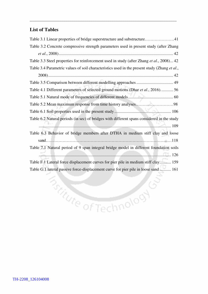
List of Tables
Table 3.1 Linear properties of bridge superstructure and substructure…………………41
Table 3.2 Concrete compressive strength parameters used in present study (after Zhang
et al., 2008) ............................................................................................................. 42
Table 3.3 Steel properties for reinforcement used in study (after Zhang et al., 2008) ... 42
Table 3.4 Parametric values of soil characteristics used in the present study (Zhang et al.,
2008) ....................................................................................................................... 42
Table 3.5 Comparison between different modelling approaches ................................... 49
Table 4.1 Different parameters of selected ground motions (Dhar et al., 2016). ........... 56
Table 5.1 Natural mode of frequencies of different models ........................................... 60
Table 5.2 Mean maximum response from time history analyses………………………98
Table 6.1 Soil properties used in the present study ...................................................... 106
Table 6.2 Natural periods (in sec) of bridges with different spans considered in the study
.............................................................................................................................. 109
Table 6.3 Behavior of bridge members after DTHA in medium stiff clay and loose
sand………………………………………………………………………………118
Table 7.1 Natural period of 9 span integral bridge model in different foundation soils
.............................................................................................................................. 126
Table F.1 Lateral force displacement curves for pier pile in medium stiff clay ........... 159
Table G.1 lateral passive force-displacement curve for pier pile in loose sand ........... 161
TH-2208_126104008

______________________________________________________________________
List of Symbols
A : A factor account for cyclic loading in sand
Ap : Area of pile
As : Area of steel
As, pro : Area of steel provide
Asw : Area of the stirrups or ties in one direction of confinement
Aw : Equivalent are of pile row
C1, C2, C3 : Coefficient as function of �
CL : Very stiff clay
D : Pile diameter
Db : Diameter of longitudinal bar
E1, E2, E3 : Stiffness of pile 1st, 2nd, and 3rd pile rows
Eeq : Equivalent elastic modulus
H : Depth below soil surface
J : Dimensionless empirical constant
Mw : Moment of magnitude
Ned : Design value of applied axial force
OL/SM : Loose sandy silt
R : Fault to site distance
Sa : Spectral acceleration
SL : Spacing of hoops or spiral
SP : Very dense sand
SP/SM : Medium dense silty sand
X : Depth below soil surface
XR : Depth below soil surface to bottom of reduced resistance zone
TH-2208_126104008

�������������
______________________________________________________________________
xx
a : The distance of CG of the concentrated load from nearest support
b1 : Breadth of concentrated area of load
bef : Effective width of the slab perpendicular to span
bw : Width Of the slab
c : Cohesion
epsc0 : Strain at compressive strength of concrete
fpcU : Crushing strength of concrete
epsU : Strain at crushing strength
fpc : Compressive strength of concrete
fyd :Design yield strength of reinforcement
l0: Effective span of main girder
p : Perimeter of pile
pu : Ultimate resistance
� : A constant having the following value depending on width of slab and l0
� : Unit weight of soil
�c: Strain at which half of maximum stress is occurring
� : Soil-wall internal friction
�k : Normalised axial force
�� : Volumetric ratio of transverse reinforcement
� : Angle of internal friction
� �d : Required confining reinforcement ratio
� �d, pro : Provided confining reinforcement ratio
TH-2208_126104008

______________________________________________________________________
Chapter 1
Introduction
1.1 Introduction
In conventional bridges, different types of bearings or supports are provided at the
locations of piers and abutments to accommodate movement arising from temperature
effects, creep and shrinkage of the bridge superstructure. In recent years, many bridges
are being constructed with monolithic action of the abutment and the superstructure.
Those bridges are known as integral abutment bridges (Fig. 1.1). The monolithic
construction of abutment and superstructure eliminates the requirement of bearings and
leads to reduction in the maintenance cost. However, the piers may support the
superstructure by means of bearings or get integrally connected with the deck (Burke,
2009). In an Integral Abutment Bridge (IAB), the abutment may rest on shallow footing
or pile foundation depending on the type of soil.
Fig. 1.1 A typical single span jointless bridge
Generally, the superstructure of an IAB is constructed of structural steel or
reinforced concrete (cast-in-situ) or prestressed concrete. Prestressed concrete and steel
superstructure integral abutments (Conboy and Stoothoff, 2005; Weakley, 2005; Maberry
TH-2208_126104008

���������������
______________________________________________________________________
2
and Camp, 2005; Lampe and Azizinamini, 2000; Arockiasamy et al., 2004) have been
constructed extensively in the past, however the design and construction details have
varied from place to place (Maruri and Petro, 2005; White et al., 2010). Several
modifications have been made in RC integral abutment and foundation design (Yannotti
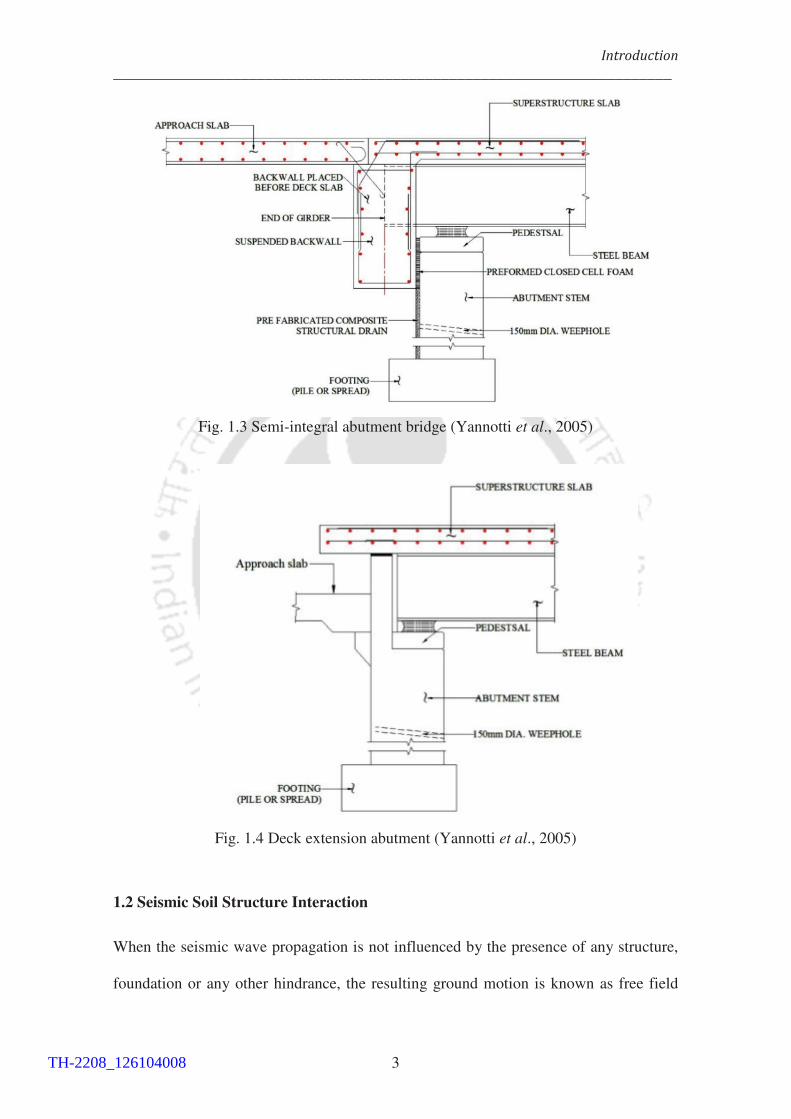
et al., 2005). For integral abutment bridges, three types of construction are possible,
namely (a) Full Integral Abutment (FIA) (Fig. 1.2), (b) Semi Integral Abutment (SIA)
(Fig. 1.3) and (c) deck extension (Weakley, 2005; Perkun and Michael, 2005; Maberry
and Camp, 2005) (Fig. 1.4). In SIA bridges, there may be partial force and moment
transfer but in FIA bridges, full transfer of moment and forces occurs from deck to
abutment. A detailed procedure to achieve complete rigid deck girder-abutment
connection has been developed in Itani and Pekcan (2011). In an IAB, the abutments and
the foundation need to be designed to accommodate both temperature effects and the
effect of earthquake shaking. Thus, Soil-Structure Interaction (SSI) plays a major role in
the overall behaviour of the IAB for the different combinations of loadings.
Fig. 1.2 Fully integral abutment bridge (Yannotii et al., 2005)
TH-2208_126104008
�����������
______________________________________________________________________
3
Fig. 1.3 Semi-integral abutment bridge (Yannotti et al., 2005)
Fig. 1.4 Deck extension abutment (Yannotti et al., 2005)
1.2 Seismic Soil Structure Interaction
When the seismic wave propagation is not influenced by the presence of any structure,
foundation or any other hindrance, the resulting ground motion is known as free field
TH-2208_126104008

�� ��������������������������������������������
______________________________________________________________________
4
motion (Kramer, 1996). If a structure is founded on solid rock then due to the extremely
high stiffness of the rock, the rock motion resembles the free field motion very closely.
Structures founded on rock are considered as fixed-base structure as the possible
translations and rotations at the base of the structure are completely restrained during
earthquake shaking. On the other hand, the same structure may respond differently when
supported on soft foundation soil. Under free field motions, the foundation will not be
able to deform, thus, the motion at the base of the structure tends to deviate from the free
field motion. Then, the dynamic response of the structure itself will induce deformation
of the supporting soil. This process, in which the dynamic response of the soil influences
the possible motion of the structure and then, the dynamic response of the structure
influences the possible motion of the soil, is referred to as Soil Structure Interaction (SSI).
Seismic waves propagate through the soil strata and finally reach the foundation of the
structure, causing it to move, as a result of which the superstructure also starts to vibrate
(JSCE, 1985). The dynamic characteristics of ground motion at the base of structure
depend on the modification of bedrock motion while propagating through the soil strata
(Dutta, 2010). Thus, it is important to know how the seismic waves propagate through
the soil medium to understand the modification of ground motion due to variation in the
soil properties. Also, the vibration characteristics of the soil medium are required to carry
out numerical modelling of wave propagation through the semi-infinite soil medium.
1.3 Major Concern and the Motivation of the Study
In an integral bridge on pile foundation, the abutments, bridge deck and the piers act like
a combined single unit due to the monolithic nature of construction. During earthquake
shaking, the seismic response of the integral bridge-foundation system depends on the
abutment-backfill interaction and soil-pile interaction. Thus, soil structure interaction
TH-2208_126104008

�����������
______________________________________________________________________
5
(SSI) needs to be considered while investigating the seismic behaviour of an integral
bridge on pile foundation. Although the SSI effects have been considered for analysing
the behaviour of an integral bridge under temperature loading in past research (Efretuei,
2013; Laman and Kim, 2010; Far et al., 2015), the influence of the modelling approaches
incorporating SSI on the seismic behaviour of the integral bridge has not been studied. A
few parametric studies have also been carried out in the past (Erhan and Dicleli, 2017;
Kong et al., 2016; Huang et al., 2008; Civjan et al., 2007) involving the effects of
different structural and geotechnical parameters on the seismic response of an integral
bridge. However, the seismic response of integral bridge with RC pile foundation needs
to be investigated in detail to prescribe seismic design guidelines for such bridges.
Also, in past earthquakes, pile foundations in several bridges have been observed
to undergo significant damages (San Fernando, 1971; Tangshan, China, 1976; Hyogoken
Nanbu, Kobe, 1995; Izimit, Turkey, 1999; Jiji, Taiwan, 1999; Athens, Greece, 1999). In
an integral bridge with pile foundation, the seismic demand on the piles below the
abutments and the piers can significantly increase with the overall length of the bridge. It
can also vary with the different types of underlying soil. Detailed investigations and
identification of such possible failures of abutment piles and pier piles are also required
as part of assessment of seismic vulnerability of the bridge. Subsequently, appropriate
retrofitting measures of pile foundations need to be studied for possible remedy. All these
provide the motivation for the present study.
1.4 Objectives of the Study
The objectives of the thesis are as follows:
TH-2208_126104008

�������������������������
______________________________________________________________________
6
• The influence of different modelling approaches on the seismic response of an integral
bridge on RC pile foundation, considering soil-structure interaction and site-specific
ground motions, is to be investigated.
• The influence of overall length of an integral bridge with RC pile foundation on its
seismic response will be studied for different types of foundation soils.
• The effectiveness of one of the retrofitting methods of pile foundation below the
abutments and the piers, by using new piles encased in jet grout, is to be studied
through numerical modelling.
1.5 Outline of the Thesis
The organization of the contents of the thesis is discussed below:
1. Chapter 1: In this chapter, an overview of integral abutment bridge and the background
for the present study, are discussed. Finally, the objectives of the present study and the
organization of the thesis are presented.
2. Chapter 2: Past research work and technical guidelines on IABs are discussed in this
chapter. Based on the past studies, the gap areas are identified and the scope of the
work is mentioned.
3. Chapter 3: In this chapter, the modelling of the integral bridge-foundation-backfill
system using continuum soil domain approach in OpenSees program, is discussed in
detail. The corresponding material properties are also elaborated. Further, the details
of the alternative spring-dashpot modelling, using Beam on Dynamic Winkler
Foundation (BDWF) approach, are also discussed.
4. Chapter 4: In this chapter, a two-dimensional site response analysis is carried out on a
free field soil column using OpenSees, STRATA and DEEPSOIL programs and the
TH-2208_126104008

�����������
______________________________________________________________________
7
results are compared. For further detailed studies, site specific ground motions are
selected using REXEL-DISP tool for a target site specific displacement spectrum.
5. Chapter 5: In this chapter, the behaviour of superstructure and substructure of an
integral bridge is determined using different modelling approaches (with and without
the SSI effects), and the comparative results are discussed in detail.
6. Chapter 6: As the overall length of an integral bridge is expected to increase the forces
and the moments in the bridge components, the influence of overall length on the
seismic behaviour of an integral bridge under site specific ground motions is studied
in this chapter.
7. Chapter 7: In this chapter, the retrofitting method for abutment and pier pile
foundations, using new piles encased in jet grout, is first discussed. The retrofitting
technique is implemented on the integral bridge with maximum overall length, as
discussed in Chapter 6, through numerical modelling in the SAP2000 program. Further,
the effectiveness of the retrofitting method is discussed considering the response of
piers and the piles for different types of foundation soils.
8. Chapter 8: In this chapter, conclusions from the present study are drawn and the
possible future scope of work is mentioned at the end.
TH-2208_126104008

�������������������������
______________________________________________________________________
8
TH-2208_126104008

______________________________________________________________________
Chapter 2
Literature Review
2.1 Introduction
In an Integral Abutment Bridge (IAB), the superstructure and the abutment are
constructed monolithically at their junction without the presence of any bearing or
expansion joint. This leads to a significant reduction in the maintenance cost of the bridge.
However, integral connection at the deck-abutment junction causes a significant change
in the bridge behaviour under thermal loading and earthquake shaking as
the superstructure (along with bridge deck and girders), abutment with foundation, wing
wall and the approach slab may act like a single unit. Different countries and the
respective Highway Agencies have adopted different guidelines for design and
construction of IABs. In the present chapter, the past research involving studies on soil-
structure interaction and design guidelines on integral abutment bridges are reviewed.
The major parameters of an IAB required for its design, namely the overall length,
skewness and loadings on the bridge are discussed first. Next, the behaviour of the
abutment including abutment-backfill interaction, and the possible numerical modelling
techniques are reviewed. Among the different types of foundation, only the pile
foundation is considered in the present study. So, past studies on soil-pile interaction and
its modelling are discussed in detail. Although, most of the bridge design guidelines in
different countries do not include provisions on soil-structure interactions, the available
prescriptions are reviewed. Finally, a few retrofitting methods for pile foundation are
discussed along with identification of gap areas and scope of the present work.
2.2 Characteristics of IAB
2.2.1 Length
TH-2208_126104008

2.2 Characteristics of IAB
______________________________________________________________________
10
The length of an IAB depends on pile capacity, soil type and abutment displacement due
to temperature variation and seismic excitation (Greimann et al., 1984). According to
temperature variation, construction methods and geological conditions, the limiting
length of IAB varies across different regions. In US, most of the states have relatively
low maximum span lengths for steel beam within 60 m and concrete beams upto 45 m
(Baptiste et al., 2011). Using pile supported stub type abutment, prestressed girder bridges
upto 244 m length and steel bridges upto 122 m length are routinely constructed (Dicleli
and Albhaisi, 2003). The maximum recommended length of bridges in cold climates is
190 m with concrete girders and 100 m with steel girders. In moderate climates, the limits
are increased to 240 m and160 m with concrete and steel girders respectively. Barr et al.
(2013) have observed that an increasing in span by a factor of two can lead to an increase
of bending moment by 60% for weak axis bending of the bridge abutment (Appendix A).
Although, long span IABs may have total span to be more than 300 m (e.g., Happy
Hollow Creek Bridge with a length of 358 m (Comisu, 2005)), currently, researches are
continuing in the direction of increasing the length of IABs considering optimisation
approach for pile shape design (Lan, 2012). As imposed seismic forces on an integral
bridge tend to increase with its overall length, proper measures should be taken before
constructing long span IBs depending on proper geological investigation and site specific
characteristics.
2.2.2 Skew angle
Skewness and curvature in IABs play a crucial role to elevate the time dependent load on
backfill soil. The maximum permitted skew angle varies according to the guidelines of
different countries, and is prescribed as (a) 30° for UK, Finland and Australia (Gibbens,
2011; White, 2007) and (b) 30°-60° in different states of USA and European countries
(Greimann et al., 1983; Puzey, 2012; Barr et al., 2013; Quinn and Civjan, 2016). In
TH-2208_126104008

Literature Review
______________________________________________________________________
11
Canada, detailed investigations are required while designing IABs with skew angle more
than 20°. However, countries like Germany do not permit construction of skewed IABs
due to possible increase of backfill earth pressure for skewed bridges (Civjan et al., 2013).
The same practice is followed in Japan due to possibility of frequent earthquake shaking.
2.2.3 Loadings on IAB
In addition to the primary load effects (dead load and live load), integral bridges are
subjected to secondary load effects due to (a) creep and shrinkage, (b) thermal gradients,
(c) Abutment-Backfill Interaction (ABI) and (d) Soil-Pile Interaction (SPI) (Arockiasamy
et al., 2004). Although, creep and shrinkage effects have been ignored by many designers
(Maruri and Petro, 2005), those effects can contribute significantly to the overall loading
on an IAB.
For pretensioned or posttensioned concrete bridges, creep, shrinkage and elastic
shortening account for changes in the internal behaviour (Liu et al., 2005; Bazant and
Panula 1980). Shrinkage of the concrete deck slab tends to impose compressive stresses
in the top flange of the girder and tensile stresses in the bottom flange (Wetmore and
Peterson, 2005). Additional shear force and bending moment arise in the superstructure
due to shrinkage of deck on the hardened superstructure girder (Arockiasamy and
Sivakumar, 2005). Most of creep and shrinkage deformations in the precast girders get
completed by the time the girders are made continuous at the time of deck slab casting.
Measurements indicate a significant shortening of the deck associated with creep and
shrinkage of the prestressed beams (Barker and Carder, 2001). But shortening tends to
get reduced after a few years of construction (Lawver et al., 2000); thus, it is not
considered to have a significant effect. Differential deck slab and girder shrinkage,
inherently shortens the superstructure and directly affects the integral abutment system.
TH-2208_126104008
2.2 Characteristics of IAB
______________________________________________________________________
12
Creep coefficients of high performance concrete tend to be less as compared to the
traditional concrete mixes (Knickerbocke et al., 2005; Roller et al., 1995).
Changes in temperature may cause significant changes in the length of bridge deck
girders. Unlike the conventional bridges, an IB does not have any expansion joint or
bearing between superstructure and abutment. Bridge displacement is affected by both
seasonal and diurnal temperature changes. Extreme temperature changes during summer
days and winter nights control the extreme displacements of an IAB (Shah et al., 2008).
Based on experimental and analytical data (BA 42/96, 2003; England et al., 2000), a limit
of seasonal movement of ±20mm for short span IABs has been prescribed for temperature
induced pressure on different types of integral abutments. Far et al., (2015) have
prescribed that during negative temperature changes, seismic force should be combined
with temperature load as contraction of IABs is more critical and it is unsafe for the
bridges, particularly located in cold earthquake prone regions.
The response due to temperature load are governed by many factors, such as type
of abutment backfill, season of backfill construction (Efretuei, 2013), abutment
displacements including translations and rotations, the type of pile and its orientation. The
effective temperature which governs the overall longitudinal movement of the bridge
depends on shade temperature, solar radiation, wind speed, material properties, surface
characteristics and section geometry. In several past studies, two major parameters,
namely (a) maximum and (b) minimum shade temperatures have been correlated with
effective bridge temperature (Volz, 2005; Emerson, 1976; BSI, 1978; Imbsen et al., 1985;
AASHTO, 1989; Girtonet al., 1991). It was postulated that the thermal expansion of a
bridge deck could be accommodated to a certain extent by cambering of the deck rather
than causing the deck to undergo hogging action (Darley and Alderman, 1995). Laman
TH-2208_126104008

Literature Review
______________________________________________________________________
13
and Kim (2010) developed temperature gradient based on axial load and bending strains
from AASHTO gradient profile.
Studies have been carried out to determine the longitudinal thermal expansion of
bridge deck, enforcing a longitudinal strain equilibrium and compatibility by collection
of bridge deck segments (Volz, 2005; ACI, 1982; Girton et al., 1991). Although the
distribution of temperature across the depth of girder is non-uniform, code provisions
(IRC:6, 2017) prescribe expressions to estimate variation of temperature considering the
same. Comparisons from various proposed thermal gradients with data accumulated from
field test indicate that the temperature gradients in AASHTO (2012) and Volz (2005)
provide reasonable upper bounds to solar radiation differentials (Abendroth et al., 2007).
The bending moment arising from thermal expansion can significantly influence the axial
capacity of the pile (Abendroth et al., 1989). During earthquake shaking, inertia forces
generated at the deck level are transmitted to the backfill through integral abutments as
well as to the soil through foundation. The deck-abutment joints are thus subjected to
high stresses under seismic loading. Dicleli and Albhaisi (2003) suggested that ABI effect
need not be considered for an IAB under negative thermal variation due to very small
displacement. However, it is strongly dependent on the type or geometry of the abutment
and do not hold good for extreme cold weather. Most of the countries in Europe and USA
prefer to consider full passive pressure behind the abutment. The intensity of the backfill
pressure behind the abutment depends on the magnitude of the bridge displacement
towards the backfill soil and strain ‘racheting’ effect of backfill due to thermal variation.
2.3 Abutment Behaviour
The total earth pressure on the abutment during an earthquake is contributed by three
components, namely (1) the static pressure due to gravity loads, (2) pressure induced due
TH-2208_126104008

2.3 Abutment Behaviour
______________________________________________________________________
14
to displacement of the wall towards the backfill from inertial loading and (3) temperature
or earthquake induced lateral pressures due to ABI (Matthewson et al., 1980). For the
analysis of integral abutment-foundation system, three different stiffness contributions
are considered, namely (a) longitudinal or translational stiffness of abutment, (b)
rotational stiffness of the abutment wall-backfill system and (c) stiffness of underlying
foundation, as shown in Fig. 2.1. By lumping various components of stiffness at different
locations in the structural model, the expressions for abutment stiffness have been derived
(Petursson and Kerokoski, 2011). Active earth pressure tends to get mobilized at a very
small lateral displacement when the abutment moves away from the backfill (Barker et
al., 1991). For practical purposes, the variation of passive earth pressure coefficient with
lateral displacement of integral abutment towards backfill can be assumed to be linear
with effect of thermal variation (Dicleli, 2000).
2.3.1 Foundation type
Usually, fixed head steel H-piles are very commonly used as foundation for the
abutments. Other than H-piles, different types of abutment foundation (Dunker and Liu,
2007) include steel pipe piles, precast concrete piles, timber piles (Kamel et al., 1996),
sheet piles (England et al., 2000) and spread footing. X-shaped (cross shaped) piles are
also used for abutment foundation below IABs in some countries of Europe (White et al.,
2010). Spread footing should be avoided for multi-span IABs due to differential
settlement. Use of batter piles for skewed IABs is not suggested in construction practice
(Hassiotis et al., 2006).
When an IAB is supported by flexible or hinged pile heads, all lateral forces are
taken by abutment backfill, bridge deck and to some extent by the flexible abutment piles.
A pinned abutment-pile connection is observed to increase the overall displacement of
the bridge significantly due to increased translation and rotation of the abutment (Dicleli
TH-2208_126104008

Literature Review
______________________________________________________________________
15
and Albhaisi, 2003) but it reduces the force transferred from superstructure to
substructure significantly (Arsoyet al., 2002).Usage of carpet wrap at pile head of
abutment piles is not sufficient to allow rotation at pile head (Abendroth et al., 2007).
The abutment supported by a single row of piles provides higher flexibility along
longitudinal direction by weak axis bending (Burke, 1993; Arockiasamy et al., 2004;
Wasserman and Walker, 1996; Nielsen and Schmeckpeper, 2001; Arsoy et al., 2002;
Quinn and Civjan, 2016; BSDC, 2017), but that also tends to increase the stresses in piles
leading to the possibility of plastic hinge formation near the pile head. This results in a
desirable behaviour for the abutment-pile system with avoidance of concrete cracking
even for skewed bridge and H-piles under thermal variation. Although H-piles are not
suggested to be oriented to mobilize strong axis bending (Abendroth and Greimann,
2005), combination of strong axis bending and stiff foundation soil reduces stresses in
piles and increase forces in concrete deck girders (Huang et al., 2008). Bahjat (2014)
observed that abutment rotation or displacement may not depend on pile orientation in
skewed IAB subjected to thermal variation. So, pile design and orientation should be
based on specific bridge situation. The design and orientation of abutment piles should
be based on specific bridge characteristics, temperature variation and the type of abutment
backfill.
TH-2208_126104008
______________________________________________________________________
Fig 2.1 Modelling of wall contribution in the stiffness of abutment (Lam and Martin, 1986).
TH-2208_126104008

Literature Review
______________________________________________________________________
17
2.3.2 Abutment backfill interaction
Abutment backfill soil should not be susceptible to get drained way during rainfall, be
frozen in winters and free from roots, sods or perishable materials. Most US states prefer
well compacted granular materials as backfill. The level of compaction behind the
abutment affects the overall response of the IAB. Earthquake-induced lateral loading can
mobilize passive soil pressure resistance through sliding or horizontal displacement of
abutment towards backfill. For walls of low heights (upto 1.5 m) it is expected that the
inertial effect under earthquake shaking should be small, thus the passive resistance is
computed using static pressure distribution (SCDOT, 2010). The Mononobe Okabe (MO)
method of determining seismic passive pressure coefficients for abutments is not
recommended due to its various limitations. Considering wall friction and soil surface
failure, seismic passive earth pressure coefficients have been suggested in past studies
(Shamsabadi, 2006; Shamsabadi et al., 2007; Anderson et al., 2008). When superstructure
inertia forces are transmitted into the backfill through abutment, adequate passive
resistance must be available to avoid translation and rotation of the abutment. It is
recommended that abutments should be designed to restrict lateral displacements upto
approximately 91mm in order to avoid severe failure during strong earthquake shaking
(AASHTO, 2002). Damping arising from ABI is significant in several experimental
studies for relatively short IABs (upto 60 m length) (Douglas and Reid, 1984).
The variation of the backfill pressure as a function of the abutment displacement
towards the backfill can be calculated from the studies carried out by Claugh and Duncan
(1991), and Petursson and Kerokoski (2011). John and Faraji (1998) compared the design
curves given in Canadian Foundation Engineering Manual (CFEM) (2006) and NCHRP
(1991) with experimental results for translation and rotation of the abutment wall. For
dense soil, design curves given in CFEM are recommended for ABI while for loose and
TH-2208_126104008

2.3 Abutment Behaviour
______________________________________________________________________
18
medium soils, the curves given in NCHRP are suitable. The equations to calculate the
coefficient of passive earth pressure which suit the NCHRP design curves has been given
by Bonczar et al. (2005). Acceptable comparisons are achieved from design curves for
dense and medium soils given in CFEM and NCHRP with the suggested expressions from
past researchers for modelling of integral abutment (Kumar, 2008). Comparison of
different design curves is given in Fig. 2.2. Caltrans (2004) has recommended the
estimation of seismic passive soil resistance behind bridge abutments based on full scale
experimental results. An approximate quasi-linear relationship between seismic passive
earth pressure and wall movement has also been established (Arsoyet al., 1999; Dicleli
and Albhaisi, 2004).
Fig. 2.2 Comparison of design curves given in different manual (Faraji et al., 1998)
‘Log-spiral’ Hyperbolic Load Deflection (HLD) curves (Fig.2.3) for seismic
passive pressure have been proposed to represent the nonlinear ABI for monotonic
TH-2208_126104008
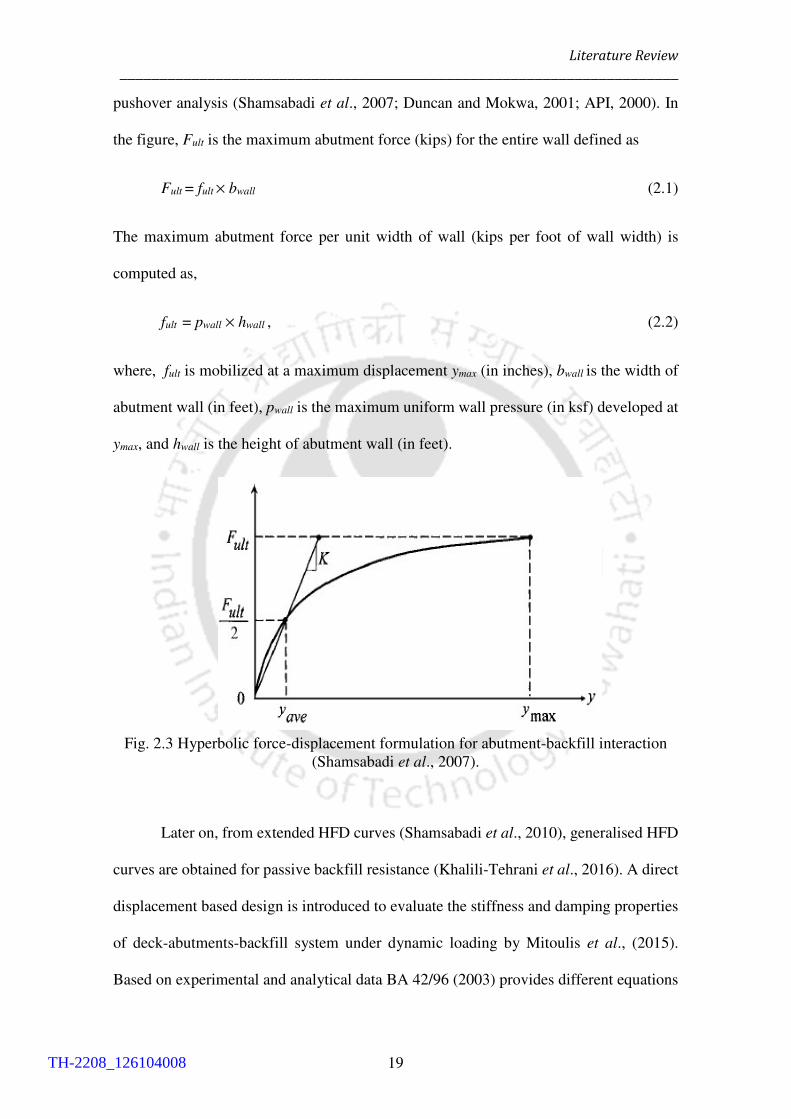
Literature Review
______________________________________________________________________
19
pushover analysis (Shamsabadi et al., 2007; Duncan and Mokwa, 2001; API, 2000). In
the figure, Fult is the maximum abutment force (kips) for the entire wall defined as
Fult = fult × bwall (2.1)
The maximum abutment force per unit width of wall (kips per foot of wall width) is
computed as,
fult = pwall × hwall , (2.2)
where, fult is mobilized at a maximum displacement ymax (in inches), bwall is the width of
abutment wall (in feet), pwall is the maximum uniform wall pressure (in ksf) developed at
ymax, and hwall is the height of abutment wall (in feet).
Fig. 2.3 Hyperbolic force-displacement formulation for abutment-backfill interaction
(Shamsabadi et al., 2007).
Later on, from extended HFD curves (Shamsabadi et al., 2010), generalised HFD
curves are obtained for passive backfill resistance (Khalili-Tehrani et al., 2016). A direct
displacement based design is introduced to evaluate the stiffness and damping properties
of deck-abutments-backfill system under dynamic loading by Mitoulis et al., (2015).
Based on experimental and analytical data BA 42/96 (2003) provides different equations
TH-2208_126104008

2.3 Abutment Behaviour
______________________________________________________________________
20
to calculate earth pressure on different types of integral abutments. The framed abutment
supports the vertical loads from the bridge and acts as a retaining wall for embankment
earth pressure. The magnitude of the passive pressure acting on the wall is significant.
The pressure coefficient K* for that abutment shown in Fig. 2.4, where K0 is earth pressure
coefficient at rest and H is the height of the abutment. The distribution of passive and
active earth pressures as per Claugh and Duncan (1991) are shown in Fig. 2.5.
Fig. 2.4 Earth pressure distributions on framed abutments (BA 42/96, 2003)
Researches have produced relatively simple and cost-effective design solutions
for reduction of irreversible movements of IAB and strain ratcheting of backfill under
thermal loading (Hassiotis et al., 2005). Additive lateral earth pressures on abutments can
be reduced by using a variety of modern design approaches, for example use of
geosynthetic reinforcement or geogrid in backfill soil (Zornberg, 2007; Tatsuoka et al.,
2014), rubber-soil mixture or reused tyre aggregates at backfill (Argyroudis et al., 2016;
Mitoulis et al., 2016; Mitoulis, 2016), buried approach slab (Wendner and Strauss, 2014),
using polyethylene sheets below approach slab to reduce friction with backfill
soil(Mistry, 2005), different ground-improvement methods (Horvath, 2000; Horvath,
TH-2208_126104008

Literature Review
______________________________________________________________________
21
2005) and updating retrofitting techniques from jointed bridge to IABs (Xue, 2013;
Jayaraman et al., 2001). Use of rubberish material with backfill soil reduces abutment top
displacement, ‘ratcheting effect’, gap between backfill and abutment and‘bump-at-the-
end-of-bridge’, as stresses and forces on overall bridge structure get reduced.
Fig. 2.5 Variation of passive earth pressure with the lateral displacement of abutment
wall (Claugh and Duncan, 1991)
For bridges, proper provisions for drainage of backfill behind the abutment need
to be provided in order to minimize the build-up of fluid pressure on abutment. In general,
a series of vertical drains is recommended rather than a single continuous drainage to
increase the efficiency of the system (Gibbens, 2011). Pipe under drains must be provided
to drain the fill from backfill and wing wall. For mechanically stabilised wall,
impermeable membrane is required surrounding the steel straps (drains) to avoid soil
contamination. Poor drainage control during construction can cause settlement of
approach slab due to erosion during rainfall, around and under the abutment and wing
walls (SBDC, 2017).
TH-2208_126104008
2.4 Soil Pile Interaction
______________________________________________________________________
22
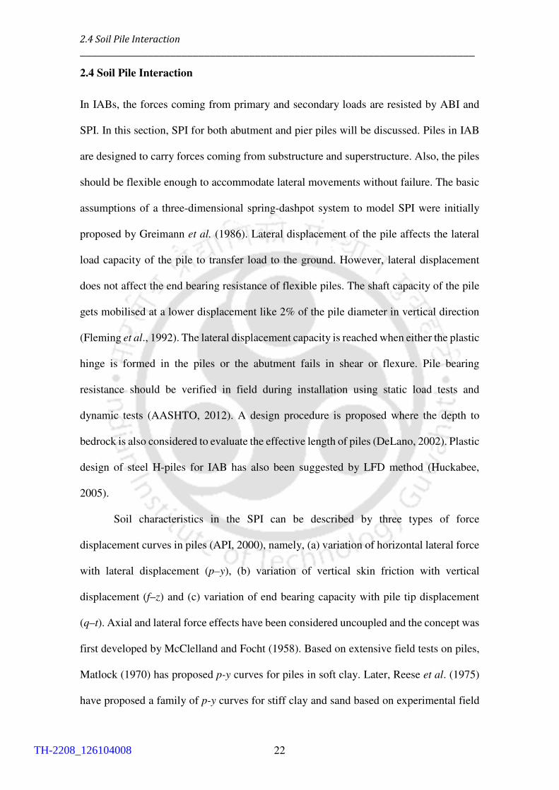
2.4 Soil Pile Interaction
In IABs, the forces coming from primary and secondary loads are resisted by ABI and
SPI. In this section, SPI for both abutment and pier piles will be discussed. Piles in IAB
are designed to carry forces coming from substructure and superstructure. Also, the piles
should be flexible enough to accommodate lateral movements without failure. The basic
assumptions of a three-dimensional spring-dashpot system to model SPI were initially
proposed by Greimann et al. (1986). Lateral displacement of the pile affects the lateral
load capacity of the pile to transfer load to the ground. However, lateral displacement
does not affect the end bearing resistance of flexible piles. The shaft capacity of the pile
gets mobilised at a lower displacement like 2% of the pile diameter in vertical direction
(Fleming et al., 1992). The lateral displacement capacity is reached when either the plastic
hinge is formed in the piles or the abutment fails in shear or flexure. Pile bearing
resistance should be verified in field during installation using static load tests and
dynamic tests (AASHTO, 2012). A design procedure is proposed where the depth to
bedrock is also considered to evaluate the effective length of piles (DeLano, 2002). Plastic
design of steel H-piles for IAB has also been suggested by LFD method (Huckabee,
2005).
Soil characteristics in the SPI can be described by three types of force
displacement curves in piles (API, 2000), namely, (a) variation of horizontal lateral force
with lateral displacement (p–y), (b) variation of vertical skin friction with vertical
displacement (f–z) and (c) variation of end bearing capacity with pile tip displacement
(q–t). Axial and lateral force effects have been considered uncoupled and the concept was
first developed by McClelland and Focht (1958). Based on extensive field tests on piles,
Matlock (1970) has proposed p-y curves for piles in soft clay. Later, Reese et al. (1975)
have proposed a family of p-y curves for stiff clay and sand based on experimental field
TH-2208_126104008

Literature Review
______________________________________________________________________
23
testing of piles. Afterwards, a unified curve for both soft and stiff clays has been defined
by Sullivan et al. (1979). Several other methods like Hansen’s theory (1963), ‘Broms’
method (1964), have also been proposed for estimation of lateral pile resistance for the
same soil conditions (Fan and Long, 2005; Shia, 2005). The most commonly used API
(2000) method has been implemented for soft clay (Matlock, 1970), stiff clay (Reese et
al., 1975) and sand (Murchison, 1983).
A thorough discussion for the determination of p-y curves is given by Wang and
Reese (1993). COM624Psoftware can beused for analysis of SPI (Wasserman and
Walker, 1996; Wasserman, 2001). This procedure is confirmed by research at University
of Tennessee (Burdette et al., 2004). The effective length of the pile is determined from
identification of the points of zero moment at several depths of pile and the longest of
these distances is used in subsequent nonlinear calculations. Previously, field tests have
been performed on driven piles to compare the ultimate strength to that computed, using
AASHTO (1996) and AISC (1996) column design equations. The results from the field
study have shown that the prescribed equations predicted overly conservative values for
the ultimate lateral bearing capacity of the piles (Ingram et al., 2003) because considering
piles as unsupported between inflection points does not take into account the influence
and support by the surrounding soil. So, measures should be taken during lateral design
of different types of concrete piles which are partially included in the current code version
(AASHTO, 2012). Prebored holes filled with flexible material and sleeve piles can be
used to prevent downdrag of piles (IDOT, 2006; Hassiotis et al., 2005).
The abutment and wing-wall may not behave as a rigid block even if abutment is
supported on flexible piles (Mourad and Tabsh, 1998).As expected, reducing the number
of piles under the abutment greatly affects the axial load on piles but it does not
significantly change the tension force in piles under the wing-walls. The axial stresses in
TH-2208_126104008

2.4 Soil Pile Interaction
______________________________________________________________________
24
the piles are not affected by the type of wing-wall and fixed or hinged abutment-pile joint.
In USA, guidelines recommend not to build piles under wing wall as it would restrict the
rotation of integral abutment system which may further induce additional forces on the
structure (White, 2008). Cantilever wing wall in the perpendicular direction of traffic and
integrally founded with abutment, can increase the forces on girders during thermal
expansion as it resists the expansion of the bridge superstructure (Paraschos, 2016; Huang
et al., 2008). The axial forces and bending moments in the deck increase and peak
moments in the piles decrease when the backfill soil is varied from loose to dense nature.
However, for H-piles, the bending moment demand increases once the foundation soil
changes from loose to dense (Faraji et al., 2000; Zhao et al., 2011). Very little work
concerning the capabilities of integral abutments founded on short piles has been carried
out. Existing design procedures preclude the use of piles below effective length because
of the assumptions which are generally based on or validated for longer piles only
(DeLano, 2002). Stresses in a pile may increase due to several reasons like, long bridge
span, stiff soil, deep girders and weak axis bending. The spatial extent of the bridge-
foundation system is large which necessitates an appropriate finite-element mesh to
provide adequate modelling resolution. So, pre-processing and output visualization in 3D
finite element (FE) analysis of the entire bridge-ground system can be quite tedious and
time consuming (Elgamal et al., 2008).
Beam on Dynamic Winkler Foundation model (BDWF) (Makris and Gazetas,
1992) has been established for SPI which states that each subdivided layer of soil should
be represented by a series of independent, discrete springs in the vertical and the
horizontal directions. The soil surrounding the pile is considered to be divided into two
zones (Hutchinson et al., 2004), namely (a) near field and (b) far field zones, as shown in
Fig. 2.6. Strong material nonlinearity is expected in the near field zone while soil
TH-2208_126104008

Literature Review
______________________________________________________________________
25
behaviour would be primarily linear elastic in the far field zone. If viscous dashpots are
modelled in parallel configuration with the nonlinear spring element (to capture hysteresis
in soil for the near-field zone) for capturing the effects of radiation damping, it is referred
as parallel radiation damping soil-modelling method (Kagawa and Kraft, 1980a, b;
Badoni and Makris, 1996). If nonlinear hysteretic spring-dashpot is placed in series with
the linear visco-elastic spring-dashpot (radiation damping), it is termed as series radiation
damping of soil modelling (Novak and Sheta, 1980). Series radiation damping method
ismore realistic as compared to the parallel radiation damping method as it avoids the
possibility of unrealistically large damping forces in the near field zone (Wang et al.,
1998). Radiation damping in the far-field soil domain of bridges occurs due to SSI and
energy dissipation of waves radiating out into soil away from the bridge foundation
(Gazetas and Dobry, 1984).
Fig. 2.6 General schematic of the finite element (FE) model used for the BNWF
analyses using the nonlinear fiber beam-column element and the nonlinear p-y element
(Hutchinson et al., 2004).
TH-2208_126104008
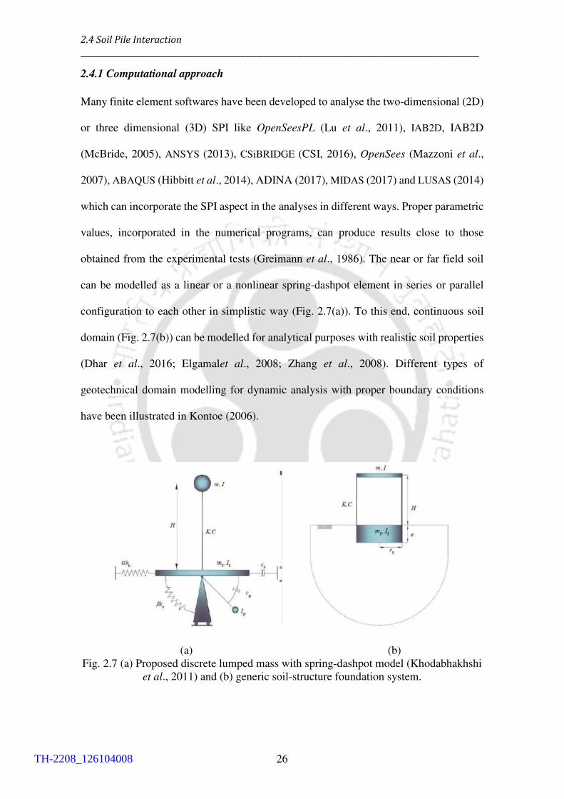
2.4 Soil Pile Interaction
______________________________________________________________________
26
2.4.1 Computational approach
Many finite element softwares have been developed to analyse the two-dimensional (2D)
or three dimensional (3D) SPI like OpenSeesPL (Lu et al., 2011), IAB2D, IAB2D
(McBride, 2005), ANSYS (2013), CSiBRIDGE (CSI, 2016), OpenSees (Mazzoni et al.,
2007), ABAQUS (Hibbitt et al., 2014), ADINA (2017), MIDAS (2017) and LUSAS (2014)
which can incorporate the SPI aspect in the analyses in different ways. Proper parametric
values, incorporated in the numerical programs, can produce results close to those
obtained from the experimental tests (Greimann et al., 1986). The near or far field soil
can be modelled as a linear or a nonlinear spring-dashpot element in series or parallel
configuration to each other in simplistic way (Fig. 2.7(a)). To this end, continuous soil
domain (Fig. 2.7(b)) can be modelled for analytical purposes with realistic soil properties
(Dhar et al., 2016; Elgamalet al., 2008; Zhang et al., 2008). Different types of
geotechnical domain modelling for dynamic analysis with proper boundary conditions
have been illustrated in Kontoe (2006).
(a) (b)
Fig. 2.7 (a) Proposed discrete lumped mass with spring-dashpot model (Khodabhakhshi
et al., 2011) and (b) generic soil-structure foundation system.
TH-2208_126104008

Literature Review
______________________________________________________________________
27
Numerical methods for analysis of soil-structure interaction can be divided into
two main categories, namely (a) Direct methods and (b) Multistep methods. In the direct
method, the entire soil-foundation-structure system is modeled and analyzed in a single
step. Free field input motions are specified along the base and sides of the model, the
resulting response of the interacting system is computed (for the finite element model)
from the equation of motion. Multistep methods use the principle of superposition to
isolate the two primary causes of soil structure interaction, namely (a) the inability of the
foundation to match the free-field deformation and (b) the effect of the dynamic response
of the structure-foundation system on the movement of supporting soil.Two types of
interactions are observed, namely (a) kinematic and (b) inertial interactions. In kinematic
interaction, earthquake shaking will cause soil displacements along both the horizontal
and the vertical directions. If a foundation on the surface of, or embedded in, a soil deposit
is so stiff that it cannot follow the free-field deformation pattern, its motion will be
influenced by kinematic interaction, even in the absence of any mass. Kinematic
interaction will occur whenever the stiffness of the foundation system impedes the
development of the free-field motions. Kinematic interaction can also induce different
modes of vibration in a structure. In inertial interaction, the masses of the structure and
the foundation are considered which play a major role in the dynamic response. If the
supporting soil is compliant, the forces transmitted to it by the foundation will produce
foundation movement that would not occur in a fixed-base structure. The effects of soil
compliance on the resulting response are due to inertial interaction.
In direct method, FE discretisation is carried out to model the structure and a
portion of the underlying soil to artificial boundary. Various such artificial boundaries
have been developed to simulate radiation of spurious waves away from the soil domain.
Kausel and Tassoulas (1981) have categorised the possible boundaries into three major
TH-2208_126104008

2.4 Soil Pile Interaction
______________________________________________________________________
28
groups, namely (a) elementary boundaries, (b) local boundaries and (c) consistent
(nonlocal) boundaries. In elementary boundaries, either zero displacements are specified
by fixing the nodes lying at the boundary or zero surface tractions are enclosed at the
boundaries. It works well when damping is present and boundary is chosen at a sufficient
distance from structure. Ghosh and Wilson (1969) have suggested that if the boundary is
kept at a distance of 3r to 4r in horizontal and 2r to 3r in vertical direction, then
satisfactory results can be obtained, where r is the radius of foundation. In local
boundaries, the degrees of freedom lying at the boundary are not coupled to each other
and are thus local in nature (Fig. 2.8(a)). The most widely used local boundary is the
standard viscous boundary suggested by Lysmer and Kulhemeyer (1969). Consistent
boundaries can transmit both types of waves, for any angle of incidence resulting in no
reflection (Fig. 2.8(b)). All the DOF lying at the boundaries are coupled, along with
frequency dependent properties of springs and dashpots. These can transmit all the waves
from the soil boundary. The only restraint imposed is that the frequency dependent
properties may not be suitable for the dynamic time-domain analysis.
(a) (b)
Fig.2.8 (a) Lysmer Viscous Boundary and (b) Consistent Boundary
In case of 2D modelling method, continuum soil domain is generally modelled
with quadrilateral or triangular FE mesh with suitable constitutive properties of soil. FE
analysis indicated that SIA offer benefits over FIA, such as reducing the pile stresses,
TH-2208_126104008

Literature Review
______________________________________________________________________
29
particularly during contraction of the bridge. In addition, interaction between the
approach fill and the foundation soil creates favourable conditions with pile stresses
(Duncan and Arsoy, 2003). FE programs also account for the gap formation at the soil-
pile and abutment-pile interfaces by introducing gap element or contact element. Zero-
thickness interface elements can be used to model soil-pile and abutment-backfill
interactions to allow slip at those interfaces (Zhang et al., 2008). Modelling of contact or
interface elements has been discussed in past studies (Hibbitt, 2014; Zhang et al., 2008;
Kolay, 2009; Gentela and Dasgupta, 2012).
Three-dimensional (3D) finite element models of IAB increase the level of
complexity in the analysis, as well as the computational requirements. However, unlike
2D models, 3D models can account for the skew effects (Deng et al., 2015) and effects
of eccentric loading. 3D soil continuum can be modelled by 8 or 20-noded brick element
in FE softwares. Discrete Element Method (DEM) can be used for numerical analysis to
model interaction between different rubber-soil mixtures and abutment (Cui and Mitoulis,
2015).
2.5 Field Studies
IABs equipped with instrumentation provide valuable insight into the behaviour of
integral piles due to loading from traffic, earth pressure forces and temperature changes.
Recently in several countries, short span old conventional bridges are updated to IABs
for better performance. Measures are taken for IABs to relieve the earth pressure on the
piles and the abutments to permit sufficient longitudinal movements. The void space
created behind the abutment can be filled with corrugated metal supported by specifically
thickened pressure relief compressible strips (Jorgenson, 1983). The piles which are
rigidly connected to the bottom of the abutment tend to bend in double curvature. To
TH-2208_126104008

2.5 Field Studies
______________________________________________________________________
30
eliminate the bending action, integral abutment and pile connection can be provided as
hinged. A schematic diagram of pile-to-cap hinged connection developed by
Anastasopoulos et al. (2008) for dynamic analysis of pile under strong earthquake
shaking (not fault related) is shown in Fig. 2.9.
Fig 2.9 Schematic of Pile-to-Cap Hinged Connection
In full IAB, internal piers may be capable of lateral movements, if not, then some
base isolation system should be arranged in between superstructure and internal piers
(Froschet al., 2005). Semi-integral abutment bridge can be constructed as hinged at the
top and bottom of abutment by neoprene bearing strip transferring the force by padded
dowel (Arsoy et al., 2004) and should be used where rigid soil and long span bridges are
necessary (Burke, 2009). In typical Australian practice for IABs, link slab at intermediate
piers joints is introduced (Connal, 2004). In New Zealand, full IABs and semi IABs are
permitted if rotational stiffness component is taken into consideration (Jamieson, 2009)
for bridges more than 60 m length. Highway overpasses less than 60 m length are suitable
for construction as IABs (Torricelli et al., 2012).
Other than proper backfill compaction, dynamic response of the bridge structure
is also governed by nonlinear inelastic response of the underlying soil during earthquake
shaking. The plastic soil deformations impose large residual displacements on the IAB
TH-2208_126104008
Literature Review
______________________________________________________________________
31
after strong earthquakes (Zhang et al., 2008; Elgamal et al., 2008). Moments in piles has
been calculated conservatively using simple beam theory and indicated that yielding of
piles have not been occurred during long term thermal variation (Brena, 2007).
Experimental results (Springman et al., 1996) suggest that loosely placed backfill should
not be used, regardless of whether or not an approach slab is used; although loose backfill
reduces the force coming on bridge during dynamic or thermal loading. To prevent
settlement of approach slab, US guidelines recommend use of drag plates or buried
approach slab with repairable special connection between slab and abutment (Frangi et
al., 2011) which is easily repairable. The strain in approach slabs does not depend on
whether the approach slab is a precast or cast-in-situ type (Phares et al., 2013). During
extreme temperature, the expansion or contraction can be accommodated at approach
slab-pavement joint in jointless bridges (Husain and Bagnariol, 2000; Mistry, 2005;
BSDCH, 2017). Sometimes, the measured earth pressures on the bridge abutments may
be quite high because of well compacted backfill (Kerokoski and Laaksonen, 2005). For
highway bridges, the optimum friction angle of the backfill soil is recommended to be
limited to 45° (BA 42/96, 2003). The density and stiffness of the backfill may increase or
decrease over the yearly cycle of expansion and contraction of integral abutments (Darley
et al., 1998). A special type of steel-concrete composite joint is proposed for IABs by
Briseghella and Zordan (2015) which is easy to construct and have shown satisfactory
response under cyclic loading. Field studies have been carried out with analytical
verifications for skewed bridges to understand detailed behaviour of skewed IABs (Deng
et al., 2015; Wright et al., 2015; Olsonet al., 2013; Quinn, 2016). Based on comparisons
of the finite element models with field studies, it can be concluded that finite element
models do provide an excellent method to approximate the behaviour of an actual integral
bridge structure.
TH-2208_126104008

2.6 Code Provisions
______________________________________________________________________
32
2.6 Code Provisions
As the AASHTO (2012) specifications have not specifically addressed the design of piles
for IABs, many state transportation agencies use in-house methods based on experiences
and empirical formulae (DeLano, 2002). So far the research on integral abutment pile
design has been aimed at simplified structural models or computational analysis to
account for stresses and displacements in piles and superstructure due to thermal variation
and dynamic forces. In past studies (Abendroth and Greimann, 1988; Abendroth,
Greimann, and Ebner, 1989; Greimann and Wolde-Tinsae, 1988), the piles have been
considered as equivalent cantilevers (Greimann et al., 1987) based on the stiffness of the
soil and pile. The same method was presented considering three capacity criteria
mentioned in AASHTO (1996), which are the capacity of the pile as a structural member,
capacity of the pile to transfer load to the ground and capacity of the ground to withstand
the load. The first assumption is a conventional elastic approach (Eurocode-8, 2005),
while the second is an inelastic approach that considers redistribution of forces. In the
elastic approach, the pile is considered as an equivalent cantilever thus, the moment,
buckling load and horizontal stiffness can be calculated with respect to the effective
length of pile during thermal expansion of superstructure.
The current AASHTO (2012) provisions do not support this assumption any more.
In the other method, piles have been considered as inelastic and redistribution of forces
due to the formation of plastic hinges can occur. The damping of integral bridges that
occurs due to the inelastic behaviour of the backfill (Caltrans, 2013) has not been
recognised by Eurocode8 (2005). Later on Mitoulis (2016) have found that damping
ratios prescribed in Eurocode8 underestimated the realistic damping values. Neglecting
the thermally induced pile stresses justifies the first-order plastic theory involving small
displacements. However, for this case to be valid, local buckling needs to be prevented.
TH-2208_126104008

Literature Review
______________________________________________________________________
33
AASHTO (2012) does not allow combination of seismic and temperature loadings. Other
than temperature variation for controlling the overall bridge movement, no specific
guideline for IAB is mentioned in Australian Bridge Design Code (Austroads, 2004). A
case study to perform static (service loads, creep and shrinkage) and dynamic analyses
(displacement based) with design of IAB is given in Wood et al. (2015) and Wood (2015)
according to NZTA (2014). According to JRA (2012), drainage layer should be provided
in the approach embankment to prevent separation and corrosion of construction joints in
presence of water. Soil susceptible to lateral spreading or liquefaction after high intensity
of earthquake is highly discouraged as backfill material. In Canada, different states’
research manuals (Husain and Bagnariol, 2000; BSDC, 2017) provide the supplement to
the requirement of CSA (2014) for design and behaviour of IABs.
2.7 Retrofitting of Pile Foundation
The failure mechanism of an RC pile is typically manifested through four possible
mechanisms, namely (a) crushing of concrete, (b) yielding of steel, (c) punching failure
at the pile cap, and (d) failure of the pile due to pull-out forces. In the past, laboratory
testing and computer modelling have been performed for analysing the causes of the
failures (Chung et al., 2006; Li et al., 2005). Generally, fracture of piles is observed to
occur along with loss of lateral support from the surrounding soil or by soil layers of
different stiffness. This type of failure in pile is very common in liquefied sand due to
large lateral displacements. The punching failure at the pile cap may occur due to
insufficient thickness of the pile cap. Pile failure due to pull out forces occurs due to lack
of adequate anchorage detailing between the pile head and the pile cap reinforcement.
The reinforcing steel in the concrete pile may get pulled out from the pile cap or the pile
shaft, causing significant deformation in pile foundation (Wang, 2015).
TH-2208_126104008

2.7 Retrofitting of Pile Foundation
______________________________________________________________________
34
Improving seismic resistance and strengthening of the foundation is generally
time consuming and cost ineffective because of various restrictions including space
limitation and installation of additional protections. Keeping in mind, the growing
necessity to revise disaster prevention specifications and designs for existing bridges
situated at high intensified earthquake zones, development of easy and cost efficient
techniques for seismic retrofit of the foundations of existing structures needs special
attentions. For a pile foundation retrofit, additional piles are driven around the perimeter,
widening the plan dimension of existing pile cap when the piles are examined for lack of
tension and compression capacity. The newly installed piles are encased together in the
pile cap to work in tension and compression so that the foundation can act as a single unit.
This conventional method becomes problematic when the construction site has limited
clearance and working space. Insufficient vertical clearance below the existing pile
foundation also complicates the mentioned retrofitting method.
One of the retrofitting procedures adopted in case of pile foundation is the
“encasement” method, a derivative form of “incremental capacity method”. The
encasement method was first adopted by Japanese engineers in severe seismic zones
(earthquake level II) with comparatively softer soil (Fukada et al., 2005; Wang, 2015). It
is a hybrid method for the seismic strengthening of existing pile foundation by
modification of the existing foundation substrate. Originally, in this retrofitting technique,
steel sheet piles are installed surrounding the existing pile cap upto a design target depth.
Then, the soil underneath the pile cap or surrounding the pile cap is replaced by
engineered grout through high pressure jet grouting. Once the substrate is solidified, the
sheet pile and injected grout act as a monolithic unit. This method increases the
unsupported length of piles and provides lateral stability to the pile group foundation by
adding passive soil pressure during earthquake shaking. The steel sheet piling at the
TH-2208_126104008

Literature Review
______________________________________________________________________
35
perimeter offers resistance to the possible overturning moment through soil-sheet pile
friction mobilized during earthquake shaking. The mentioned retrofitting technique is
easy to repair at the later stage of failure and suggest a cost-effective solution for seismic
retrofitting.
Instead of sheet piles, precast RC piles can be embedded into jet grout surrounding
the pile or pile cap upto a target design depth to strengthen the lateral load carrying
capacity of existing pile foundation (Wang, 2015). The schematic diagram of the pile
embedded into jet grouting is shown in Fig. 2.10 (modified after He et al. (2016)).
Fig. 2.10 Schematic of jet-grouting reinforced pile (He et al., 2016); where, hg = height
of jet grout, dp = diameter of pile and dg = diameter of grout.
2.8 Summary
The salient aspects from the review of the past studies are summarized below:
• Highway overpasses and short span foot bridges (upto 60m span) should be constructed
as IABs and can be retrofitted from jointed bridges to jointless bridges easily. Most of
the countries (except earthquake-prone countries like Japan) permit skew angle of 30°
in IABs to construct unlike USA, where some states have permitted a skewness of 45°-
60° for jointless bridges.
TH-2208_126104008

2.8 Summary
______________________________________________________________________
36
• Most conventional approach even in cold weather is weak axis bending of H-piles in
concrete bridges. In moderate climate, strong axis bending of H-piles in concrete or
steel bridge is permissible within stiff soil.
• Series radiation damping method for BDWF can be appropriate for carrying out
numerical studies considering soil-pile interaction. Based on comparisons of the finite
element models with field experiments, it can be concluded that finite elements models
do provide uncompromising results to approximate the behaviour of an actual bridge
structure.
• To mitigate the stress and forces in the overall integral ‘abutment-backfill-deck-
foundation’ system during earthquake shaking, rubber-soil mixtures or ‘mechanically
stabilised’ geosynthetic reinforced soil as backfill can be used. Backfill should be well
compacted and should not get drained away during rainfall and should be free from
frozen soil, roots, sods or other decomposable material. Apart from deck drains, a
series of vertical drainage should be better than one continuous drainage because fill
pressure could directly communicate with the abutment structure.
• Backfill and foundation soil density have different influence on the structural
behaviour of an IAB. The forces and moments in the deck increase and peak moments
in the piles get reduced when the compaction is varied from loose to dense backfill
soil. However, the bending moment demand in HP-piles tends to increase once the
nature of foundation soil changes from loose to dense.
• Approach slab-pavement joint and wing wall parallel to traffic could be used to reduce
passive pressures by accommodating sufficient movement of integral abutment. Best
results on their behaviour and design should be obtained by monitoring of completed
projects in the past.
TH-2208_126104008

Literature Review
______________________________________________________________________
37
• Comparisons of various proposed thermal gradients with data accumulated from the
test girders indicated that the temperature gradients in AASHTO LRFD (2012) provide
reasonable upper bound to thermal variation.
2.9 Gap Areas
Based on the literature review, the possible gap areas are identified below:
• Latest codes like AASHTO (2012) prescribe adoption of ‘Broms’ Method (1964) for
design of piles under lateral loading. Special design criteria for piles below abutments
of IABs have not been prescribed anywhere and mandate detailed investigations with
reference to the different geological conditions. More studies should be carried out on
the influence of thermal and seismic load combinations on the behaviour of an IAB.
• Most of the IABs have been constructed on H-pile foundation. Seismic behaviour of
an integral bridge on RC pile foundation has not been investigated previously.
Comparison of bridge behaviour on RC pile and H-pile foundation is still required to
be carried out with proper geotechnical investigation.
• The seismic behaviours of an IB incorporating simplistic spring-dashpots and soil
continuum, have not been compared in any past study. Though, the simplistic model is
easy to analyse and more conventional to build, still the analysis of an integral bridge
on detailed soil domain-foundation system is expected to give detailed insight on the
effects of SSI on structural response.
• Though researches are going on to increase the limiting length of IBs, but the effect of
overall length on the seismic behaviour of IB has not been carried out.
• Abutment-pile foundation-backfill system plays a key role in load transfer and energy
dissipation. From the field studies, it has been seen either the failure of piles or the
TH-2208_126104008

2.10 Scope of Present Work
______________________________________________________________________
38
failure of backfill soil may lead to the failure of the entire integrated system, thus,
detailed numerical studies are required for ABI.
• The performance of possible retrofitting techniques for RC pile foundation need to be
investigated through extensive field studies and numerical modelling.
• The possibility of pile foundation of an integral bridge sustaining large displacement
and forces during SSI, needs to be investigated.
2.10 Scope of Present Work
The scope of the present study is mentioned as follows:
• Influence of different approaches of numerical modelling, considering soil structure
interaction, on the seismic behaviour of an integral bridge with RC pile foundation.
• Investigation on the effect of overall length of an integral bridge with RC pile
foundation on its seismic behaviour in different types of foundation soil.
• Comparison of seismic behaviour of an integral bridge on RC pile foundation using
spring-dashpot modelling approach and the detailed soil domain modelling approach.
• To study the influence of “in-cap encasement” method of retrofitting, using numerical
modelling, on the seismic behaviour of pile foundation below an integral bridge.
TH-2208_126104008

______________________________________________________________________
Chapter 3
Modelling
3.1 Introduction
It is generally accepted in earthquake engineering practice that dynamic soil-structure
interaction plays a beneficial role in the seismic response of structures by reducing the
seismic demand on the structure. For this reason, seismic analysis of structures is often
carried out either without considering the effect of the underlying soil, i.e., considering
an infinitely rigid foundation soil, or with simplified soil-foundation-structure interaction
using spring dashpot systems (e.g., Gazetas, 1991). Only in very special cases, the
nonlinear response at the soil-foundation-structure interaction is considered, although it
was proven in past studies to affect significantly the overall structural response (e.g.,
Boulanger et al., 1999; Figini and Paolucci, 2017).
Creation of fully coupled models including soil, foundation and structure,
properly accounting for their nonlinear behaviour, requires significant attention and
expertise; further the numerical simulations are often computationally costly. Therefore,
the practice on this fully coupled approach is limited and commonly used only for
important structures such as dams (Chuhan et al., 1998) and bridges (Shamsabadi et al.,
2007). Besides, the impact of different modelling assumptions of the soil-structure
interaction on the overall structural response, encompassing the nonlinearities of the soil
response and of the soil-foundation interaction, still deserves additional clarification. In
the present study, the different modelling approaches are investigated for a benchmark
case of a bridge model which is “inspired” by the Humboldt Bay Middle Channel
(HBMC) Bridge, California, USA. The seismic response of the original HBMC bridge
has been already discussed in the past studies (Zhang et al., 2008; Elgamal et al., 2008);
TH-2208_126104008
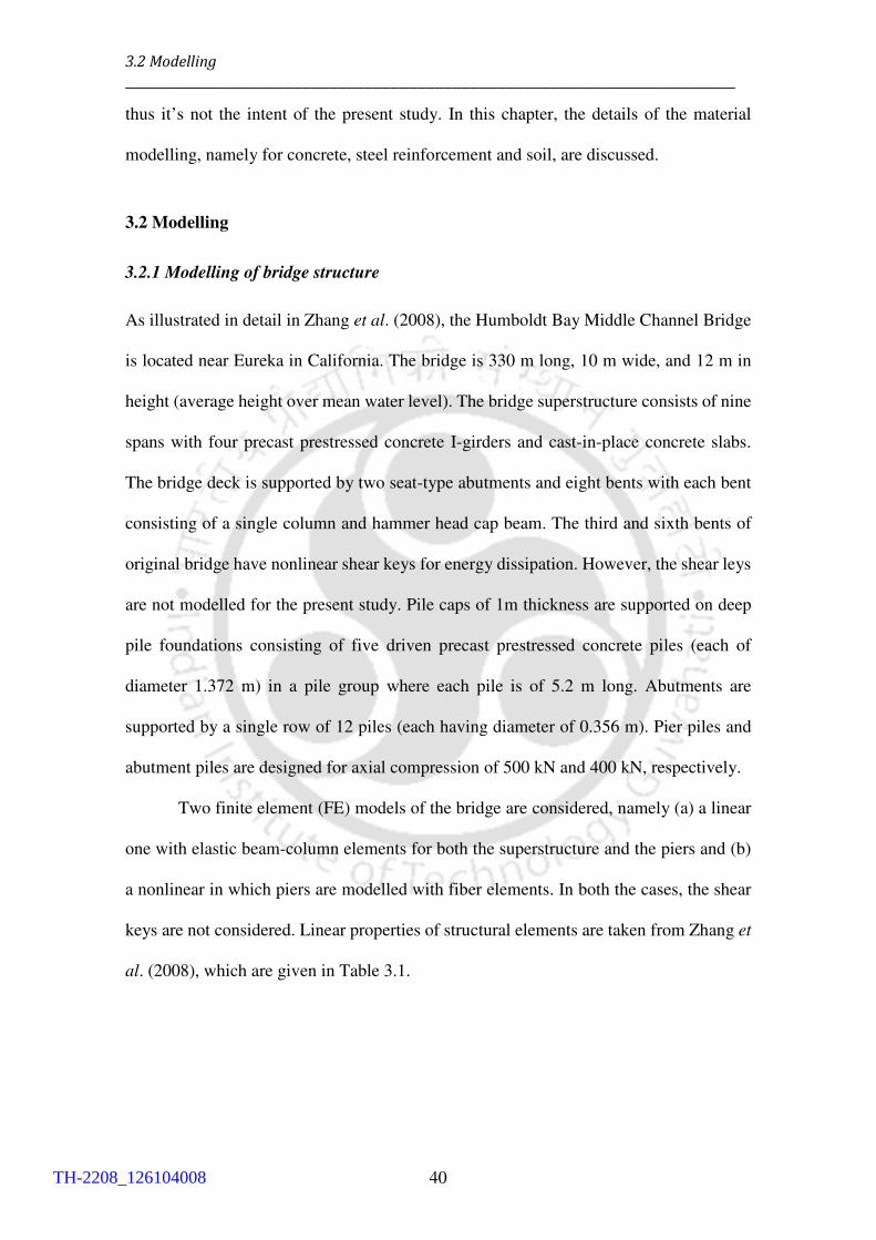
3.2 Modelling
_____________________________________________________________________
40
thus it’s not the intent of the present study. In this chapter, the details of the material
modelling, namely for concrete, steel reinforcement and soil, are discussed.
3.2 Modelling
3.2.1 Modelling of bridge structure
As illustrated in detail in Zhang et al. (2008), the Humboldt Bay Middle Channel Bridge
is located near Eureka in California. The bridge is 330 m long, 10 m wide, and 12 m in
height (average height over mean water level). The bridge superstructure consists of nine
spans with four precast prestressed concrete I-girders and cast-in-place concrete slabs.
The bridge deck is supported by two seat-type abutments and eight bents with each bent
consisting of a single column and hammer head cap beam. The third and sixth bents of
original bridge have nonlinear shear keys for energy dissipation. However, the shear leys
are not modelled for the present study. Pile caps of 1m thickness are supported on deep
pile foundations consisting of five driven precast prestressed concrete piles (each of
diameter 1.372 m) in a pile group where each pile is of 5.2 m long. Abutments are
supported by a single row of 12 piles (each having diameter of 0.356 m). Pier piles and
abutment piles are designed for axial compression of 500 kN and 400 kN, respectively.
Two finite element (FE) models of the bridge are considered, namely (a) a linear
one with elastic beam-column elements for both the superstructure and the piers and (b)
a nonlinear in which piers are modelled with fiber elements. In both the cases, the shear
keys are not considered. Linear properties of structural elements are taken from Zhang et
al. (2008), which are given in Table 3.1.
TH-2208_126104008
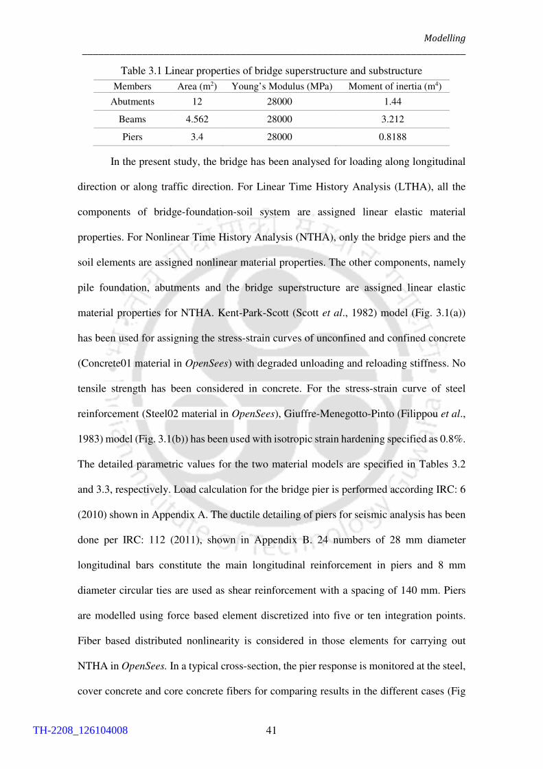
Modelling
______________________________________________________________________
41
Table 3.1 Linear properties of bridge superstructure and substructure
Members Area (m2) Young’s Modulus (MPa) Moment of inertia (m4)
Abutments 12 28000 1.44
Beams 4.562 28000 3.212
Piers 3.4 28000 0.8188
In the present study, the bridge has been analysed for loading along longitudinal
direction or along traffic direction. For Linear Time History Analysis (LTHA), all the
components of bridge-foundation-soil system are assigned linear elastic material
properties. For Nonlinear Time History Analysis (NTHA), only the bridge piers and the
soil elements are assigned nonlinear material properties. The other components, namely
pile foundation, abutments and the bridge superstructure are assigned linear elastic
material properties for NTHA. Kent-Park-Scott (Scott et al., 1982) model (Fig. 3.1(a))
has been used for assigning the stress-strain curves of unconfined and confined concrete
(Concrete01 material in OpenSees) with degraded unloading and reloading stiffness. No
tensile strength has been considered in concrete. For the stress-strain curve of steel
reinforcement (Steel02 material in OpenSees), Giuffre-Menegotto-Pinto (Filippou et al.,
1983) model (Fig. 3.1(b)) has been used with isotropic strain hardening specified as 0.8%.
The detailed parametric values for the two material models are specified in Tables 3.2
and 3.3, respectively. Load calculation for the bridge pier is performed according IRC: 6
(2010) shown in Appendix A. The ductile detailing of piers for seismic analysis has been
done per IRC: 112 (2011), shown in Appendix B. 24 numbers of 28 mm diameter
longitudinal bars constitute the main longitudinal reinforcement in piers and 8 mm
diameter circular ties are used as shear reinforcement with a spacing of 140 mm. Piers
are modelled using force based element discretized into five or ten integration points.
Fiber based distributed nonlinearity is considered in those elements for carrying out
NTHA in OpenSees. In a typical cross-section, the pier response is monitored at the steel,
cover concrete and core concrete fibers for comparing results in the different cases (Fig
TH-2208_126104008
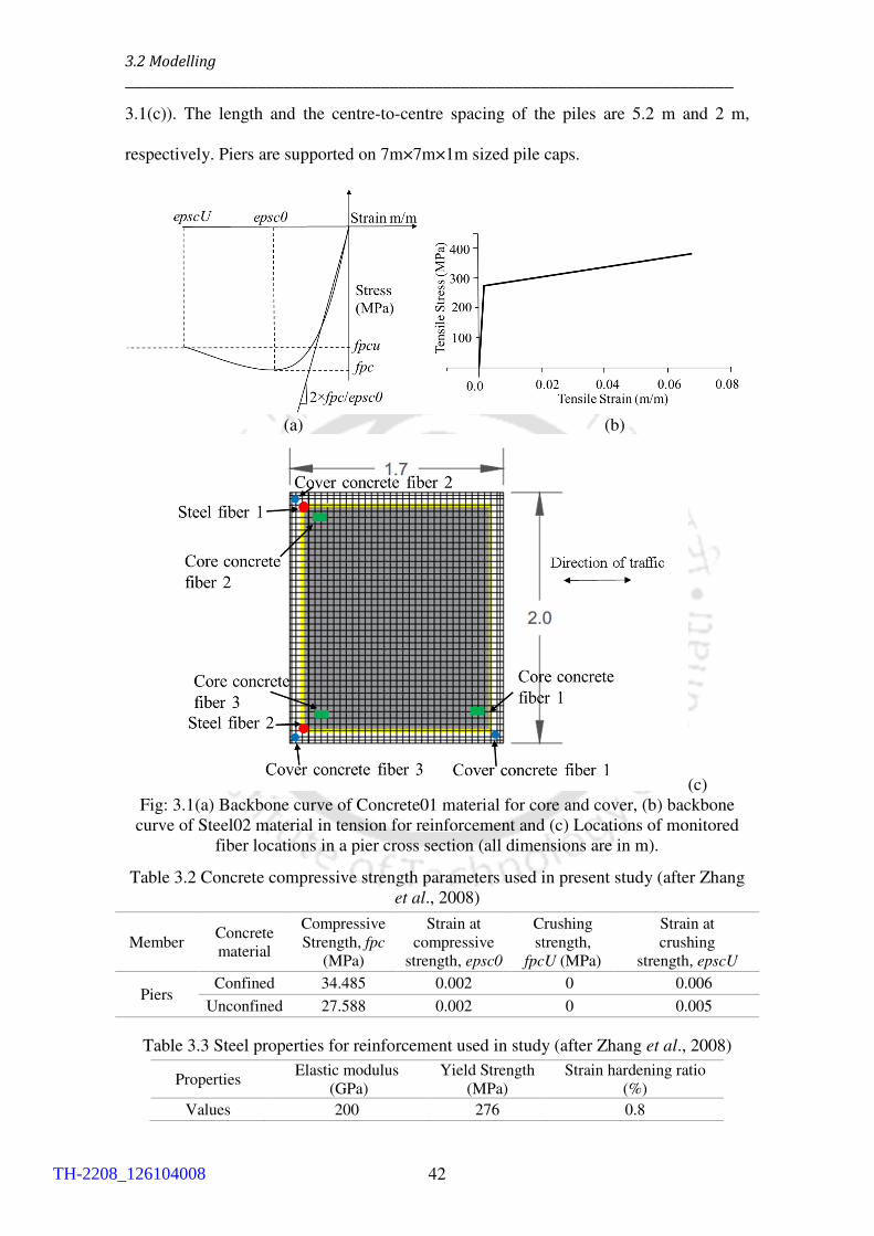
3.2 Modelling
_____________________________________________________________________
42
3.1(c)). The length and the centre-to-centre spacing of the piles are 5.2 m and 2 m,
respectively. Piers are supported on 7m×7m×1m sized pile caps.
(a) (b)
(c)
Fig: 3.1(a) Backbone curve of Concrete01 material for core and cover, (b) backbone
curve of Steel02 material in tension for reinforcement and (c) Locations of monitored
fiber locations in a pier cross section (all dimensions are in m).
Table 3.2 Concrete compressive strength parameters used in present study (after Zhang
et al., 2008)
Member Concrete
material
Compressive
Strength, fpc
(MPa)
Strain at
compressive
strength, epsc0
Crushing
strength,
fpcU (MPa)
Strain at
crushing
strength, epscU
Piers Confined 34.485 0.002 0 0.006
Unconfined 27.588 0.002 0 0.005
Table 3.3 Steel properties for reinforcement used in study (after Zhang et al., 2008)
Properties Elastic modulus
(GPa)
Yield Strength
(MPa)
Strain hardening ratio
(%)
Values 200 276 0.8
TH-2208_126104008

Modelling
______________________________________________________________________
43
3.2.2 Modelling of soil and foundation
Two-dimensional soil modelling has been carried out in OpenSees (McKenna, 2008). Soil
domain is 1500 m wide (evaluated through iterations) and 220 m in depth (Fig. 3.2). The
soil domain consists of 4 different layers, as shown in the 1D soil column in Fig. 3.2 (a),
having the static and dynamic properties summarized in Table 3.4. Modelling parameters
have been taken from Zhang et al. (2008). Pressure independent multi-yield material has
been used to describe the soil behaviour through a formulation based on the multi-surface
plasticity concept with associative flow rule, inbuilt in OpenSees. The yield surfaces are
of the Von Mises type (Prevost, 1985). Since total stress analyses have been carried out,
any direct consequence of significant excess pore water pressure generation has been
naturally neglected in the present study. For nonlinearities in soil domain, variations of
shear modulus degradation and damping ratio with shear strain curves are adopted as per
the proposition of Darendeli (2001), which are shown in Figs. 3.2(b) and 3.2(c),
respectively. The lateral boundary conditions of the soil domain have been implemented
by tied degrees of freedom (TDOF) (Elgamal et al., 2008; Kontoe et al., 2007) at the two
lateral ends of the domain. This implies that the soil domain follows the behaviour of a
2D shear beam constraints, in which the horizontal response is predominant than the
vertical response. At the base level, classical Lysmer and Kuhlemeyer (1969) type
absorbing boundary conditions are applied in the horizontal direction by properly
calibrating the dashpot coefficients along with the classical vertical displacement has
been restrained. The base input motion has been given in the horizontal direction to study
the horizontal response of soil-structure system. Pile group stiffness has been analysed
from Mokwa and Duncun (2000) and modelled as an equivalent pile group (Appendix
C). Abutment backfill soil’s dynamic properties have been kept the same as loose silty
sand (OL/SM). To model the abutment-backfill interaction, no gap or interface elements
TH-2208_126104008
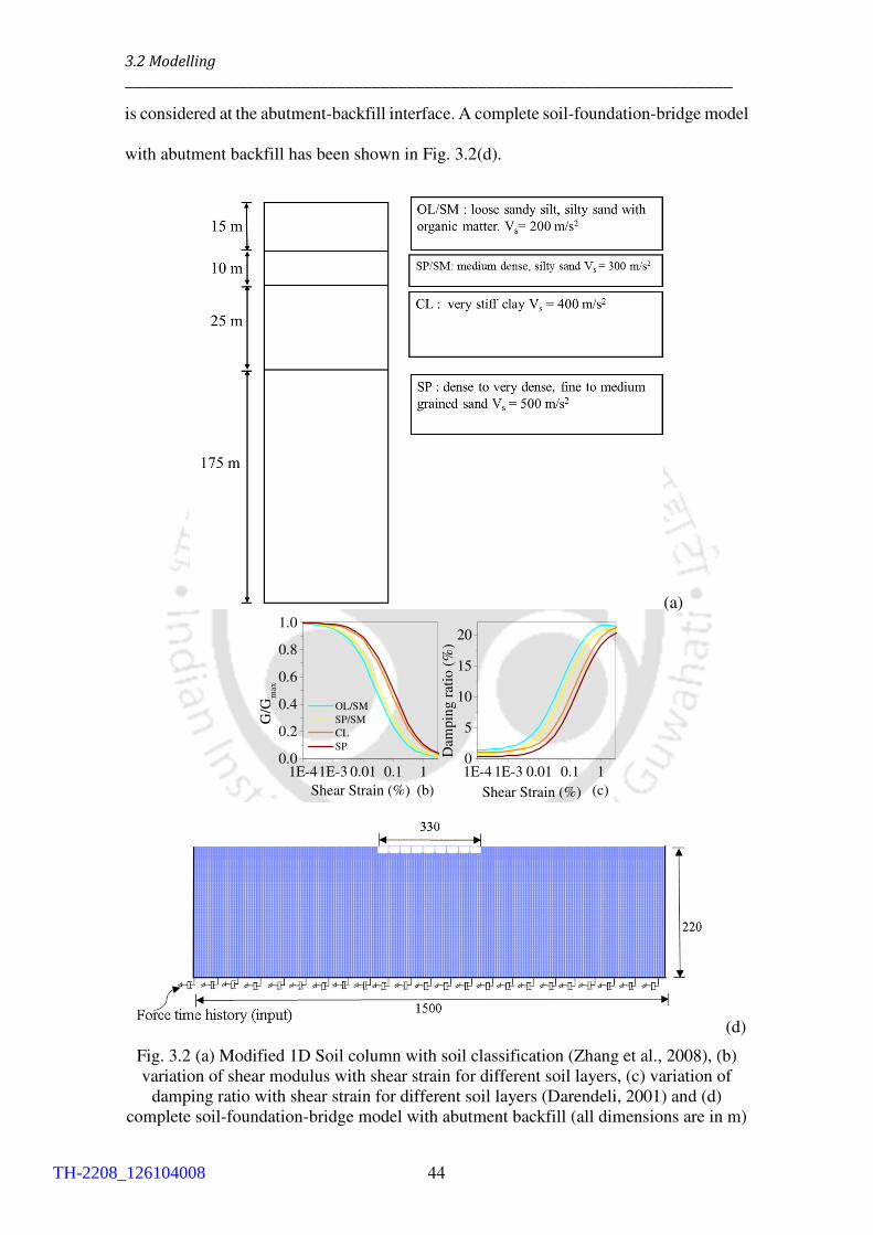
3.2 Modelling
_____________________________________________________________________
44
is considered at the abutment-backfill interface. A complete soil-foundation-bridge model
with abutment backfill has been shown in Fig. 3.2(d).
(a)
(d)
Fig. 3.2 (a) Modified 1D Soil column with soil classification (Zhang et al., 2008), (b)
variation of shear modulus with shear strain for different soil layers, (c) variation of
damping ratio with shear strain for different soil layers (Darendeli, 2001) and (d)
complete soil-foundation-bridge model with abutment backfill (all dimensions are in m)
1E-41E-3 0.01 0.1 10.0
0.2
0.4
0.6
0.8
1.0
(c)
OL/SM
SP/SM
CL
SP
G/G
max
Shear Strain (%) (b)
1E-4 1E-3 0.01 0.1 10
5
10
15
20
Dam
pin
g r
atio
(%
)
Shear Strain (%)
TH-2208_126104008

Modelling
______________________________________________________________________
45
Table 3.4 Parametric values of soil characteristics used in the present study (Zhang et al., 2008)
3.2.3 Modelling of spring-dashpot system
For the spring-dashpot model, the soil domain below the foundation is replaced by
suitable springs for modelling the behaviour of the foundation soil. The force-
displacement curves for the nonlinear springs in the near-field zone are assigned to
represent lateral load bearing capacity, vertical skin friction and pile tip axial load
carrying capacity (API rp2a, 2000). . To incorporate soil-pile interaction, spring-dashpots
have been modelled to represent the near-field and the far field effects of the soil domain.
In the near field soil, nonlinear damping has been taken care by hysteresis damping. The
springs in the lateral and the vertical directions are modelled in parallel configuration to
represent lateral load bearing capacity and skin friction of pile surface respectively.
Although soil mass has not been considered in the spring-dashpot model, far field soil
stiffness and radiation damping have been modelled from the coefficients provided in
Gazetas and Dobry (1984). Far field spring-dashpots have been modelled in series with
near field nonlinear spring-dashpots (Fig. 3.3(a)). Far field spring and dashpots are
modelled in parallel configuration. At the end of far field spring-dashpots, free field
motions have been applied at the corresponding depth of piles. Abutment backfill
interaction (ABI) is modelled by assigning nonlinear springs (Fig. 3.3(b)) behind the
abutment wall. The abutment has been considered as ‘frame type’ and the corresponding
Soil
layer
Elastic properties Nonlinear properties
Maximum
shear modulus
(MPa)
Poisson’s
ratio
Total unit
weight
(t/m3)
Undrained
strength,
(MPa)
Shear modulus
ratio
(Figs. 3.3(b)
and (c))
Plasticity
Index
OL/SM 76 0.45 1.9 0.030 Cyan Line 10
SP/SM 171 0.45 1.9 0.012 Yellow Line 0
CL 288 0.45 1.8 0.100 Orange Line 30
SP 525 0.45 2.1 0.053 Brown Line 0
TH-2208_126104008

3.2 Modelling
_____________________________________________________________________
46
springs are modelled at a spacing of 1m along the height of the abutment. The nonlinear
force-deformation curves of the springs are obtained from BA 42/96 (2003). In the
analysis, Rayleigh damping is considered as 5% at the frequencies of 0.5Hz and 5.0Hz
(Fig. 3.3(c)). From past studies (Granas, 2016; Brødbæk et al., 2009; Monkul, 2008), it
has been proven that API force-displacement curves overestimate the soil stiffness. So,
implementing API curves in bridge with spring-dashpot model tends to enhance the
imposed forces on the piles and other bridge members, leading to a conservative estimate
of the response. Thus, to reduce this error, 10% Rayleigh damping has been used in
spring-dashpot models. In Fig. 3.4, at different depth of piles and abutment backwall,
force-displacement curves are plotted to implement SPI and ABI in the spring-dashpot
models built in OpenSees. The outer pile and the middle pile from the intermediate pile
group are denoted as Pile_1 and Pile_2, respectively.
Under a suitable set of input ground motions from past earthquake records, the
impact is studied on the overall structural response of the following modelling
assumptions: (i) free field input at the base of fixed base bridge (only B_FF); (ii) SSI
input at the base of fixed base bridge (only B_SSI); (iii) full scale SSI model which
includes soil domain, foundation and bridge with and without backfill soil (full SSI with
BA model and full SSI no BA model, respectively) and (iv) bridge model with foundation
and spring–dashpots elements to represent soil with and without backfill (FB_SD with
BA model and FB_SD no BA model, respectively). In Table 3.5, all the modelling
assumptions with proper specifications are given for different types of models considered
for this study.
TH-2208_126104008

Modelling
______________________________________________________________________
47
(a)
(b)
1.5 3.0 4.5 6.00.0
2.5
5.0
Fundamental frequency
full SSI no BA
B_FF
FB_SD no BA
Ray
leig
h D
ampin
g (
%)
frequency, Hz (c)
Fig. 3.3 Schematic diagram of (a) soil-pile interaction , (b) abutment-backfill interaction
and (c) Rayleigh damping considered for analysis (For the notations refer to Table 5.1).
TH-2208_126104008
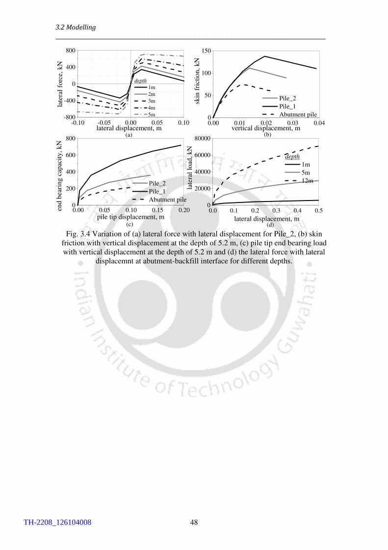
3.2 Modelling
_____________________________________________________________________
48
-0.10 -0.05 0.00 0.05 0.10-800
-400
0
400
800
skin
fri
ctio
n,
kN
(d)(c)
(b)
depth 1m
2m
3m
4m
5m
late
ral
forc
e, k
N
(a)
0.00 0.01 0.02 0.03 0.040
50
100
150
Pile_2
Pile_1
Abutment pile
Pile_2
Pile_1
Abutment pile
0.00 0.05 0.10 0.15 0.200
200
400
600
800
en
d b
eari
ng
cap
acit
y,
kN
vertical displacement, mlateral displacement, m
pile tip displacement, m0.0 0.1 0.2 0.3 0.4 0.5
0
20000
40000
60000
80000
lat
eral
lo
ad,
kN
lateral displacement, m
depth 1m
5m
12m
Fig. 3.4 Variation of (a) lateral force with lateral displacement for Pile_2, (b) skin
friction with vertical displacement at the depth of 5.2 m, (c) pile tip end bearing load
with vertical displacement at the depth of 5.2 m and (d) the lateral force with lateral
displacemnt at abutment-backfill interface for different depths.
TH-2208_126104008

Modelling
______________________________________________________________________
49
Table 3.5 Comparison between different modelling approaches
Model Boundary conditions (BC)
of vertical members
Soil Abutment
backfill
Input Motion
only B_FF Base of the bridge’s vertical
members are fixed
No soil Not present Free field soil
surface motion at
the base of piers
only B_SSI Base of the bridge’s vertical
members are fixed in
translation and rotation
No soil Not present Input motion at
base of piers from
the base of piers
of SSI model
full SSI no BA
Base of the bridge’s vertical
members have same BC in
horizontal and vertical
direction to pile cap
connecting node
Linear or nonlinear
continuum soil
domain
Not present Rock outcrop
motion at the base
of soil domain
full SSI with BA
Base of the bridge’s vertical
members have same BC in
horizontal and vertical
direction to pile cap
connecting node
Linear or nonlinear
continuum soil
domain
Continuum
backfill soil
Rock outcrop
motion at the base
of soil domain
lin str+nl soil no BA
model
Same as full SSI no BA model (piers are linear)
nonlinear continuum
soil domain
Not present Rock outcrop
motion at the base
of soil domain
nl str+lin soil no BA
model
Same as full SSI no BA model (piers are nonlinear)
Linear continuum
soil domain
Not present Rock outcrop
motion at the base
of soil domain
FB_SD no BA
Base of vertical members
have no restraints (piers are
nonlinear)
Soil stiffness and
damping represented
by equivalent
nonlinear/linear
springs and dashpots
Not present Free field input
motion at different
depth of piles
FB_SD with BA
Base of vertical members
have no restraints (piers are
nonlinear)
Soil stiffness and
damping represented
by equivalent
nonlinear/linear
springs and dashpots
Equivalent
springs
represent
backfill soil
Free field input
motion at different
depth of piles and
abutment backwall
TH-2208_126104008

3.2 Modelling
_____________________________________________________________________
50
TH-2208_126104008
______________________________________________________________________
Chapter 4
Site Response Analysis and Selection of Ground Motions
4.1 Introduction
The seismic response of a structure depends on the site-specific characteristics of the
underlying founding medium and the sets of possible site-specific ground motions of that
area. In the present chapter, the response of a soil column for the particular bridge site,
mentioned in Chapter 3, is determined under a Ricker wavelet applied at the bedrock
level. Further, the selection of site specific ground motions from REXEL-DISP tool for
time history analysis (THA) for the bridge-foundation-soil system is also discussed.
4.2. Site Response Analysis (SRA)
Before performing time history analysis, a Site Response Analysis (SRA) is carried out
for the bridge site. A 1D soil column of 220 m depth (Fig. 3.2 (a)) with proper linear and
nonlinear soil properties (Table 3.4) is modelled. Under various strong ground motions,
local site effects have been established as an important factor (Caballero et al., 2012). In
probabilistic seismic hazard analysis, ground motion data are collected over specific
geographical area and the local site condition is one of the dominant factors influencing
the seismic wave propagation and evaluation of the site-specific seismic hazard for a
particular earthquake. The open source computational programs STRATA (Kotke et al.,
2013) and DEEPSOIL (Hashash et al., 2016) are used to compare the site response
performed in OpenSees. Three types of SRA have been performed, namely (a) linear site
response analysis (LSRA), (b) equivalent linear site response analysis (ELSRA) and (c)
nonlinear sire response analysis (NSRA). In ELSRA, linear elastic properties of the soil
layers are used and these elastic properties are updated through iterative procedure
depending on the amount of computed shear deformation. The final iteration step is still
TH-2208_126104008

4.2. Site Response Analysis (SRA)
______________________________________________________________________
52
fully linear elastic with equivalent elastic parameters which approximates the nonlinear
response for that specific soil layer. In the NSRA, the dynamic wave equation with
nonlinear stress-strain relationship is solved directly. LSRA and ELSRA have been
carried out in frequency domain in STRATA. It computes the response for vertically
propagating, horizontally polarized shear waves through horizontal soil layers. OpenSees
performs the analysis using implicit Newmark beta method. The computer program
DEEPSOIL v5.0 has been used to compare OpenSees response for 1D linear and nonlinear
analyses in time domain. The two codes differ in the nonlinear modelling of soil column,
i.e., OpenSees considers nested plasticity concept (Figs. 4.1(a) and 4.1(b)), while in
DEEPSOIL a backbone curve is accompanied with unloading and reloading curves (Fig.
4.2 (c)). Variations of the hyperbolic model are adopted to represent the backbone curve
of the soil along with the extended unloading-reloading Masing rules (Masing, 1926) to
model hysteretic behaviour (Hashash et al., 2016) in DEEPSOIL. Masing rules and
extended Masing rules (Pyke, 1979; Vucetic, 1990) are used in conjunction with the
backbone curve to describe the energy dissipation characteristics (i.e., damping ratio) and
cyclic degradation behaviour of soil. The Rayleigh damping (RD) is prescribed as 2% at
0.2 Hz and 20 Hz, in OpenSees and DEEPSOIL for linear and nonlinear SRA as low strain
material damping. A Ricker wavelet of PGA as 0.2 g (with fmax = 2 Hz and maximum
amplitude at t0 = 1 sec) has been applied as bedrock input motion.
TH-2208_126104008
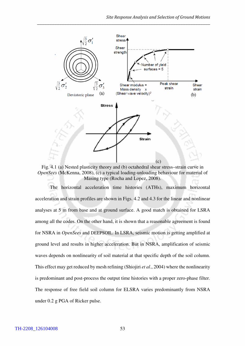
Site Response Analysis and Selection of Ground Motions
______________________________________________________________________
53
(c)
Fig. 4.1 (a) Nested plasticity theory and (b) octahedral shear stress–strain curve in
OpenSees (McKenna, 2008), (c) a typical loading-unloading behaviour for material of
Masing type (Rocha and Lopez, 2008).
The horizontal acceleration time histories (ATHs), maximum horizontal
acceleration and strain profiles are shown in Figs. 4.2 and 4.3 for the linear and nonlinear
analyses at 5 m from base and at ground surface. A good match is obtained for LSRA
among all the codes. On the other hand, it is shown that a reasonable agreement is found
for NSRA in OpenSees and DEEPSOIL. In LSRA, seismic motion is getting amplified at
ground level and results in higher acceleration. But in NSRA, amplification of seismic
waves depends on nonlinearity of soil material at that specific depth of the soil column.
This effect may get reduced by mesh refining (Shiojiri et al., 2004) where the nonlinearity
is predominant and post-process the output time histories with a proper zero-phase filter.
The response of free field soil column for ELSRA varies predominantly from NSRA
under 0.2 g PGA of Ricker pulse.
TH-2208_126104008
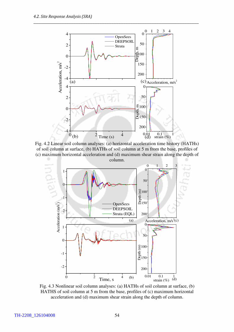
4.2. Site Response Analysis (SRA)
______________________________________________________________________
54
200
150
100
50
00 1 2 3 4
-4
-2
0
2
4
0 2 4-4
-2
0
2
4
0.01 0.1 1
200
150
100
50
0
(d)
(c)
(b) D
epth
, m
Acceleration, m/s2
OpenSees
DEEPSOIL
Strata
Acc
ele
rati
on, m
/s2
Time (s)
Dep
th, m
strain (%)
(a)
Fig. 4.2 Linear soil column analyses: (a) horizontal acceleration time history (HATHs)
of soil column at surface, (b) HATHs of soil column at 5 m from the base, profiles of
(c) maximum horizontal acceleration and (d) maximum shear strain along the depth of
column.
200
150
100
50
00 1 2 3
-2
-1
0
1
0 2 4
-2
-1
0
1
0.01 0.1 1
200
150
100
50
0
Depth
(m
)
Acceleration, m/s2
OpenSees
DEEPSOIL
Strata (EQL)
Acc
eler
atio
n (
m/s
2)
(d)
(c)
(b)Time, s
(a)
Dep
th (
m)
strain (%) Fig. 4.3 Nonlinear soil column analyses: (a) HATHs of soil column at surface, (b)
HATHS of soil column at 5 m from the base, profiles of (c) maximum horizontal
acceleration and (d) maximum shear strain along the depth of column.
TH-2208_126104008
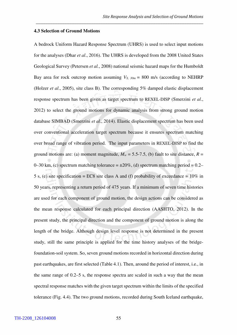
Site Response Analysis and Selection of Ground Motions
______________________________________________________________________
55
4.3 Selection of Ground Motions
A bedrock Uniform Hazard Response Spectrum (UHRS) is used to select input motions
for the analyses (Dhar et al., 2016). The UHRS is developed from the 2008 United States
Geological Survey (Petersen et al., 2008) national seismic hazard maps for the Humboldt
Bay area for rock outcrop motion assuming VS, 30m = 800 m/s (according to NEHRP
(Holzer et al., 2005), site class B). The corresponding 5% damped elastic displacement
response spectrum has been given as target spectrum to REXEL-DISP (Smerzini et al.,
2012) to select the ground motions for dynamic analysis from strong ground motion
database SIMBAD (Smerzini et al., 2014). Elastic displacement spectrum has been used
over conventional acceleration target spectrum because it ensures spectrum matching
over broad range of vibration period. The input parameters in REXEL-DISP to find the
ground motions are: (a) moment magnitude, Mw = 5.5-7.5, (b) fault to site distance, R =
0–30 km, (c) spectrum matching tolerance = ±20%, (d) spectrum matching period = 0.2–
5 s, (e) site specification = EC8 site class A and (f) probability of exceedance = 10% in
50 years, representing a return period of 475 years. If a minimum of seven time histories
are used for each component of ground motion, the design actions can be considered as
the mean response calculated for each principal direction (AASHTO, 2012). In the
present study, the principal direction and the component of ground motion is along the
length of the bridge. Although design level response is not determined in the present
study, still the same principle is applied for the time history analyses of the bridge-
foundation-soil system. So, seven ground motions recorded in horizontal direction during
past earthquakes, are first selected (Table 4.1). Then, around the period of interest, i.e., in
the same range of 0.2–5 s, the response spectra are scaled in such a way that the mean
spectral response matches with the given target spectrum within the limits of the specified
tolerance (Fig. 4.4). The two ground motions, recorded during South Iceland earthquake,
TH-2208_126104008
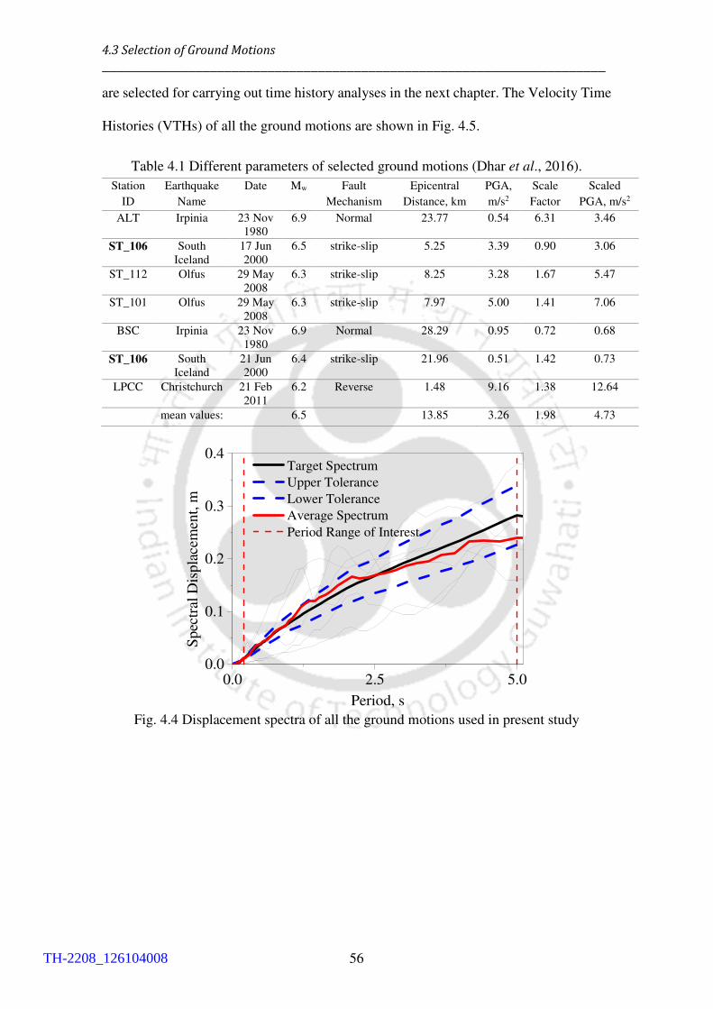
4.3 Selection of Ground Motions
______________________________________________________________________
56
are selected for carrying out time history analyses in the next chapter. The Velocity Time
Histories (VTHs) of all the ground motions are shown in Fig. 4.5.
Table 4.1 Different parameters of selected ground motions (Dhar et al., 2016).
Station
ID
Earthquake
Name
Date Mw Fault
Mechanism
Epicentral
Distance, km
PGA,
m/s2
Scale
Factor
Scaled
PGA, m/s2
ALT Irpinia 23 Nov
1980
6.9 Normal 23.77 0.54 6.31 3.46
ST_106 South
Iceland
17 Jun
2000
6.5 strike-slip 5.25 3.39 0.90 3.06
ST_112 Olfus 29 May
2008
6.3 strike-slip 8.25 3.28 1.67 5.47
ST_101 Olfus 29 May
2008
6.3 strike-slip 7.97 5.00 1.41 7.06
BSC Irpinia 23 Nov
1980
6.9 Normal 28.29 0.95 0.72 0.68
ST_106 South
Iceland
21 Jun
2000
6.4 strike-slip 21.96 0.51 1.42 0.73
LPCC Christchurch 21 Feb
2011
6.2 Reverse 1.48 9.16 1.38 12.64
mean values: 6.5 13.85 3.26 1.98 4.73
0.0 2.5 5.00.0
0.1
0.2
0.3
0.4 Target Spectrum
Upper Tolerance
Lower Tolerance
Average Spectrum
Period Range of Interest
Spec
tral
Dis
pla
cem
ent,
m
Period, s Fig. 4.4 Displacement spectra of all the ground motions used in present study
TH-2208_126104008

Site Response Analysis and Selection of Ground Motions
______________________________________________________________________
57
0 20 40 60
-0.6
-0.3
0.0
0.3
0.6
0 20 40 60 0 20 40 60
0 20 40 60
-0.6
-0.3
0.0
0.3
0.6
time, s
time, s
time, s
Velo
city
, m
/s
0 20 40 60 0 20 40 60
0 20 40 60
-0.6
-0.3
0.0
0.3
0.6
Fig. 4.5 Velocity time histories of all the seven ground motions used in the present
study.
TH-2208_126104008

4.3 Selection of Ground Motions
______________________________________________________________________
58
TH-2208_126104008

______________________________________________________________________
Chapter 5
Seismic Analysis of RC Integral Bridge
5.1 Introduction
In the present chapter, the influence of different modelling approaches is investigated on
an RC integral bridge with pile foundation. The bridge geometry are considered similar
to the Humboldt Bay Middle Channel (HBMC) bridge in California, the seismic response
of which was already presented in the past (Zhang et al., 2008; Elgamal et al., 2008). The
analysis of the different bridge-foundation-soil models are carried out using the program
OpenSees with the parametric values and ground motion details discussed in Chapters 3
and 4, respectively.
5.2 Analysis
All the considered assumptions of different types of models have been given in Table 3.5.
During the first part of analysis, three different types of models have been considered
without abutment backfill, namely (a) only B_FF (Fig. 5.1), (b) only B_SSI (Fig. 5.1) and
(c) full SSI no BA (Fig. 5.2)). In the second part, linear response of bridge with possible
nonlinear behaviour of soil (lin str+nl soil no BA model) and nonlinear response of bridge
with possible linear behaviour of soil (nl str+lin soil no BA model) are compared. In the
third or final part, the response of full SSI no BA model is compared with the response of
full SSI with BA model. Similarly, the response of full SSI with/no BA models are
compared with the response of FB_SD with/no BA models. In full SSI no BA model, four
different soil layers and vertical mesh bias are also shown in Fig. 5.2. The material
properties of the different layers in the soil domain are shown in Figs. 3.2(b) and 3.2(c).
The fundamental natural frequencies of vibration for the different models are
compared in Table 5.1. Natural frequencies of only soil domain and full SSI no BA model
TH-2208_126104008

5.2 Analysis
______________________________________________________________________
60
have been obtained by applying Ricker pulse of PGA as 0.001m/s2 at the base of the soil
domain and monitoring the seismic motion at the soil surface. From the amplification
ratio of soil surface motion and input motion, the frequencies at which first three
amplified spikes are obtained, have been considered as natural frequencies of the first
three modes. From the comparison, only B_FF model’s fundamental frequency is 2.619
Hz and reflects the maximum lateral stiffness amongst all the models. Whereas, only soil
domain and full SSI no BA model have similar natural frequencies in the first mode
because in those two models, the mass of the soil tends to dominate the behaviour of the
overall model under natural vibration. But in the 2nd and the 3rd modes, stiffness of bridge
structure also participates in the natural modes of vibration.
Table 5.1 Natural mode of frequencies of different models
Models f1 , Hz* f2 , Hz* f3 , Hz*
only B_FF 2.62 5.01 8.73
Only soil domain 0.79 0.87 0.95
full SSI no BA 0.79 1.21 1.4
FB_SD no BA 2.05 4.46 4.76 *f1, f2, f3 represent natural frequencies of 1st, 2nd and 3rd modes of vibration
( a)
Fig. 5.1 Schematic diagram of only B_FF/SSI model in OpenSees
TH-2208_126104008

Seismic Analysis of RC Integral Bridge
______________________________________________________________________
61
Fig. 5.2 Details of full SSI no BA model in OpenSees: (a) overall schematic diagram and
(b) locations in soil domain for monitoring response (all dimensions are in m).
5.3 Time History Analyses of only B_FF/SSI and full SSI no BA models
Among the seven selected ground motions from REXEL-DISP (Smerzini et al., 2014), two
chosen ground motions (denoted as GM#1 and GM#2 further in the text), are used to
discuss the results at different stages of analysis in the present study with the PGAs of
3.06 m/s2 (Fig. 5.3(a)) and 0.725 m/s2 (Fig. 5.3(b)). The fundamental natural frequencies
of the different models are marked on the Fourier transform plots of GM#1 and GM#2 in
Figs. 5.3(c) and 5.3(d) respectively, to investigate the influence of the ground motions on
the structural response with correlated natural frequencies of the studied models. Fourier
content of GM#1 is significantly higher than GM#2. In GM#2, similar amount of energy
is distributed over the entire frequency range. In linear time history analysis (LTHA),
only B_FF model is the stiffest and full SSI no BA model is the most flexible one among
the other models considered for the comparison in Table 5.1. From Figs. 5.3(c) and 5.3(d),
the dominant frequency range of the ground motions can’t be specified. Almost similar
seismic energy content can be found in low and high frequency ranges for both the GMs.
Location#1
Location#2
(a)
(b)
TH-2208_126104008
5.3 Time History Analyses of only B_FF/SSI and full SSI no BA models
______________________________________________________________________
62
So, natural frequencies of the models can’t be correlated with dominant period range of
the GMs directly.
-4
-2
0
2
4
Acc
eler
atio
n,
m/s
2
(a)
PGA 3.06 m/s2
0 10 20 30 40
-0.5
0.0
0.5
Time, s
PGA 0.725 m/s2
(b)
0.1 1 100.0
0.5
1.0
1.5
Fundamental frequencies
FB_SD no BA B_FF full SSI no BA
(d)
(c)0.0
0.5
1.0
1.5
Frequency, Hz
Fouri
er A
mpli
tude,
m/s
Fig. 5.3 Rock outcrop earthquake (scaled) ground motions (a) GM#1 and (b) GM#2;
Fourier amplitudes of (c) GM#1 and (d) GM#2 with fundamental frequencies (marked)
for the different models.
5.3.1. Structural response
From the LTHA, the pier response is found to be the maximum at the locations of the first
and the eighth piers. This is due to the location of those piers adjacent to the abutments
and higher forces are transmitted to the piers during the linear elastic behavior of the
abutments. Figures 5.4(a) and 5.4(b) show the bridge response at the top of eighth pier
for the three different models in Linear Time History Analysis (LTHA) under GM#1 and
GM#2, respectively. From the Shear Force Time History (SFTH), expectedly the only
B_FF model shows maximum response for the bridge piers due to high accelerations
TH-2208_126104008

Seismic Analysis of RC Integral Bridge
______________________________________________________________________
63
introduced at the completely restrained ends of the piers and the abutments. As only B_SSI
and full SSI no BA models have the same inputs at the bottom of each pier, similar
response is obtained for those two models. This indicates given for the same input
motions at the end of piers and abutments, the response of the bridge-foundation system
is governed by the inertial response of the bridge itself, rather than the kinematic
interaction between the foundation and the surrounding soil. The peak response from
different cases almost occur at the same time in only B_SSI and full SSI no BA models. In
only B_FF model, the peak shear force (SF) is 5,427 kN at 7.47 s and for the other two
cases the peaks are at 6.265 s and 6.44 s time instants with the SF values of 4,038 kN and
3,661 kN, respectively. Under GM#2 in Fig. 5.4 (b), the peaks of SFTHs are in similar
order as in Fig. 5.4 (a). Figs. 5.4(c) and 5.4(d) show normalized Fourier transforms (FTs)
of SFTHs plotted in Figs. 5.4(a) and 5.4(b), respectively. The FTs of the SFTHs are
normalized with respect to the peak amplitude value from all the six Fourier transforms,
which corresponds to the unit value after normalization in only B_FF model’s peak
Fourier amplitude (Fig. 5.4(c)). Normalized FT of only B_FF model carries the highest
seismic force, forming a quite sharp peak as compared to the other two models under both
ground motions in frequency domain. In Fig. 5.4(a), peaks of only B_FF, only B_SSI and
full SSI no BA models are at 2.65 Hz, 2.23 Hz and 2.24 Hz, respectively. Full SSI no BA
model’s peak is at lower frequency with lesser Fourier amplitude. The frequency shift of
peak amplitudes from 2.65 Hz to 2.24 Hz means that in presence of foundation soil, full
SSI no BA model is the most flexible one and its SFTH contains a reduced content in
frequency distribution.
Velocity Time Histories (VTHs) at eighth pier top have been monitored to
investigate the overall response at deck level in Figs. 5.5(a) and 5.5(b) under GM#1 and
GM#2, respectively. The deck is axially very stiff which causes the superstructure to
TH-2208_126104008
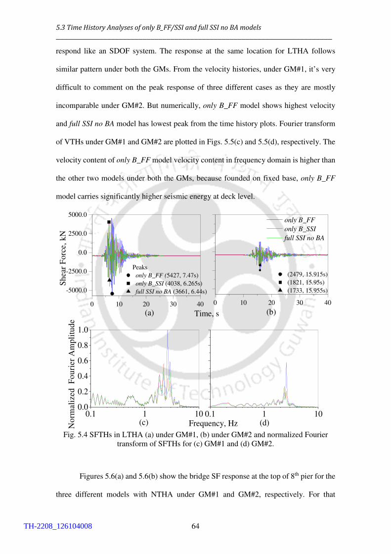
5.3 Time History Analyses of only B_FF/SSI and full SSI no BA models
______________________________________________________________________
64
respond like an SDOF system. The response at the same location for LTHA follows
similar pattern under both the GMs. From the velocity histories, under GM#1, it’s very
difficult to comment on the peak response of three different cases as they are mostly
incomparable under GM#2. But numerically, only B_FF model shows highest velocity
and full SSI no BA model has lowest peak from the time history plots. Fourier transform
of VTHs under GM#1 and GM#2 are plotted in Figs. 5.5(c) and 5.5(d), respectively. The
velocity content of only B_FF model velocity content in frequency domain is higher than
the other two models under both the GMs, because founded on fixed base, only B_FF
model carries significantly higher seismic energy at deck level.
0 10 20 30 40
-5000.0
-2500.0
0.0
2500.0
5000.0
(2479, 15.915s)
(1821, 15.95s)
(1733, 15.955s)
Peaks
only B_FF (5427, 7.47s)
only B_SSI (4038, 6.265s)
full SSI no BA (3661, 6.44s)
Sh
ear
Fo
rce,
kN
Time, s
0 10 20 30 40
only B_FF only B_SSI full SSI no BA
(a) (b)
0.1 1 100.0
0.2
0.4
0.6
0.8
1.0
0.1 1 10(c)N
orm
aliz
ed
Fo
uri
er A
mp
litu
de
Frequency, Hz (d)
Fig. 5.4 SFTHs in LTHA (a) under GM#1, (b) under GM#2 and normalized Fourier
transform of SFTHs for (c) GM#1 and (d) GM#2.
Figures 5.6(a) and 5.6(b) show the bridge SF response at the top of 8th pier for the
three different models with NTHA under GM#1 and GM#2, respectively. For that
TH-2208_126104008

Seismic Analysis of RC Integral Bridge
______________________________________________________________________
65
analysis, nonlinearity gets developed in bridge piers and foundation soil for the
appropriate models. Due to material nonlinearity in pier and foundation soil, seismic
energy dissipation due to hysteretic damping occurs and overall system tends to get more
flexible. Significant energy dissipation occurs in the inelastic piers that leads to the
reduction in the overall response of the bridge. For all the three models, the peak response
in NTHA gets reduced by 65–70% as compared to the response during LTHA under
GM#1 for all the three models. In NTHA, the only B_FF model shows the maximum
values of the peak shear force under both GMs. The same is reflected in the variation of
Fourier amplitude of the shear force response for the three models (Figs. 5.6(c) and
5.6(d)) under GM#1 and GM#2, respectively. For the full SSI no BA model, the peak
Fourier amplitude gets shifted from 2.24 Hz (for LTHA) to 0.54 Hz (for NTHA) under
GM#1 (Fig. 5.6(c)) which implies increased deformability of the nonlinear model during
dynamic analysis.
0 10 20 30 40
Vel
oci
ty,
m/s
Peak (0.70)
Peak (0.74)
Peak (0.76)
Time, s0 10 20 30 40
(b)
only B_FF only B_SSI full SSI no BA
(a)
Fig. 5.5 Velocity time histories (VTHs) in LTHA at the top of 8th pier from LTHA (a)
under GM#1 and (b) under GM#2; Fourier amplitude of VTHs (c) under GM#1 and (d)
under GM#2.
0.1 1 100
3
6
9
12
0.1 1 10(c)
Fo
uri
er A
mpli
tude,
m
Frequency, Hz (d)
TH-2208_126104008
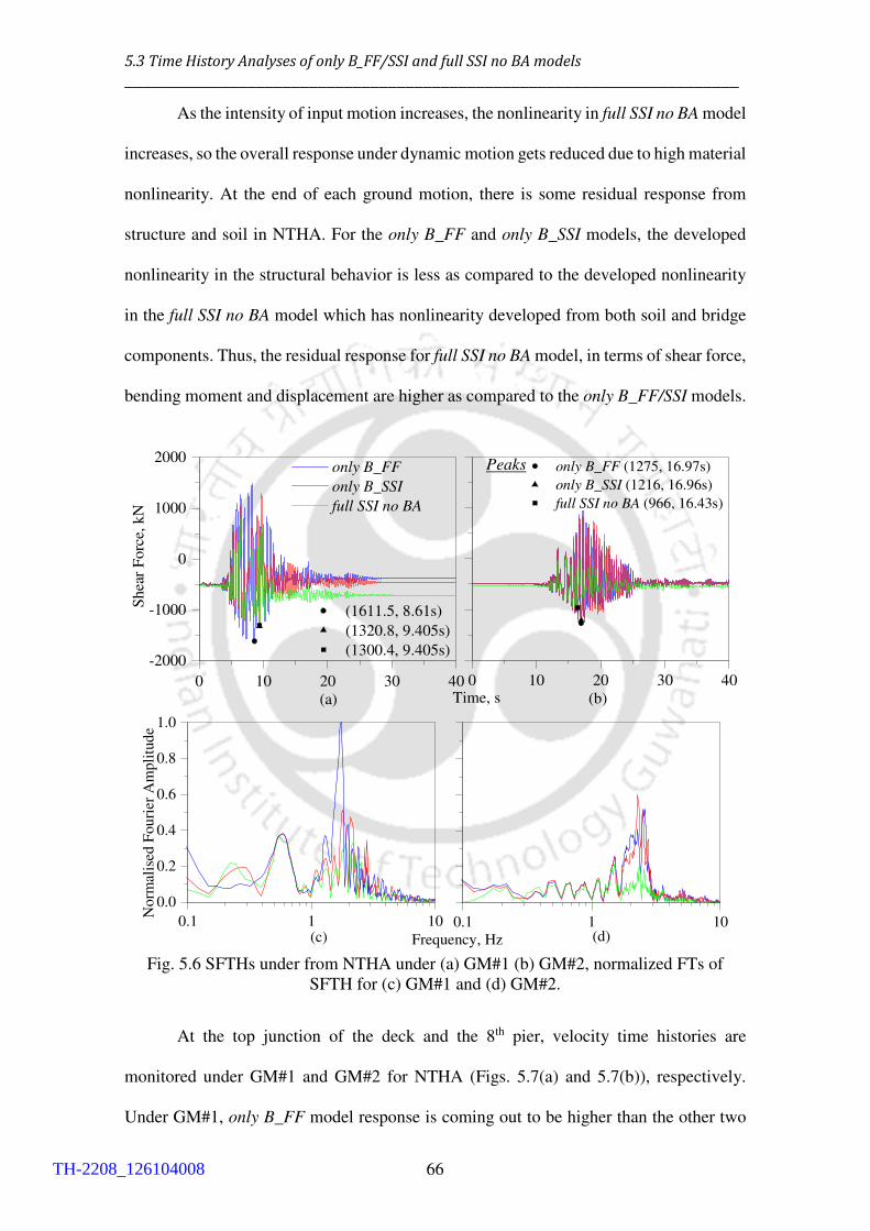
5.3 Time History Analyses of only B_FF/SSI and full SSI no BA models
______________________________________________________________________
66
As the intensity of input motion increases, the nonlinearity in full SSI no BA model
increases, so the overall response under dynamic motion gets reduced due to high material
nonlinearity. At the end of each ground motion, there is some residual response from
structure and soil in NTHA. For the only B_FF and only B_SSI models, the developed
nonlinearity in the structural behavior is less as compared to the developed nonlinearity
in the full SSI no BA model which has nonlinearity developed from both soil and bridge
components. Thus, the residual response for full SSI no BA model, in terms of shear force,
bending moment and displacement are higher as compared to the only B_FF/SSI models.
0 10 20 30 40
Shea
r F
orc
e, k
N
only B_FF (1275, 16.97s)
only B_SSI (1216, 16.96s)
full SSI no BA (966, 16.43s)
Peaks
0 10 20 30 40
-2000
-1000
0
1000
2000
(1611.5, 8.61s)
(1320.8, 9.405s)
(1300.4, 9.405s)
only B_FF only B_SSI full SSI no BA
Time, s(a) (b)
0.1 1 10
0.0
0.2
0.4
0.6
0.8
1.0
(d)(c)
No
rmal
ised
Fou
rier
Am
pli
tud
e
Frequency, Hz
0.1 1 10
Fig. 5.6 SFTHs under from NTHA under (a) GM#1 (b) GM#2, normalized FTs of
SFTH for (c) GM#1 and (d) GM#2.
At the top junction of the deck and the 8th pier, velocity time histories are
monitored under GM#1 and GM#2 for NTHA (Figs. 5.7(a) and 5.7(b)), respectively.
Under GM#1, only B_FF model response is coming out to be higher than the other two
TH-2208_126104008
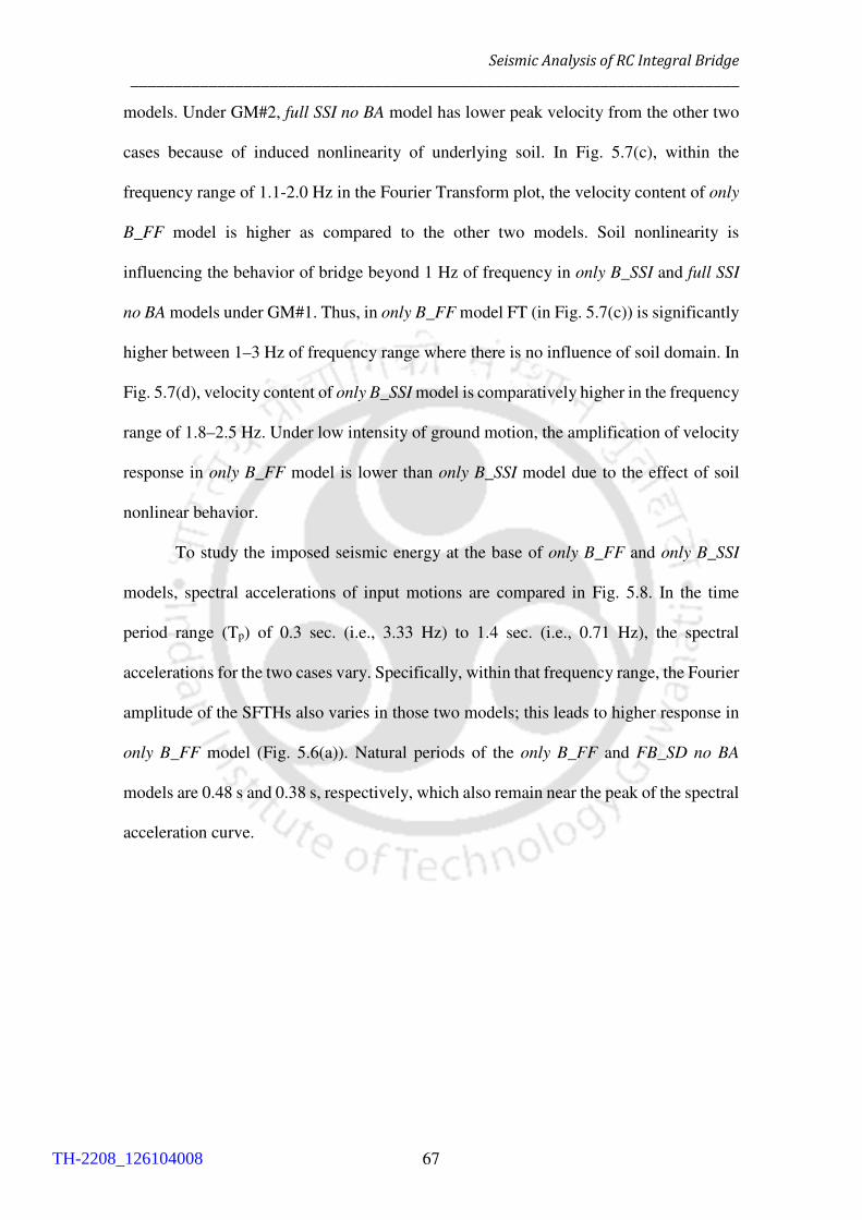
Seismic Analysis of RC Integral Bridge
______________________________________________________________________
67
models. Under GM#2, full SSI no BA model has lower peak velocity from the other two
cases because of induced nonlinearity of underlying soil. In Fig. 5.7(c), within the
frequency range of 1.1-2.0 Hz in the Fourier Transform plot, the velocity content of only
B_FF model is higher as compared to the other two models. Soil nonlinearity is
influencing the behavior of bridge beyond 1 Hz of frequency in only B_SSI and full SSI
no BA models under GM#1. Thus, in only B_FF model FT (in Fig. 5.7(c)) is significantly
higher between 1–3 Hz of frequency range where there is no influence of soil domain. In
Fig. 5.7(d), velocity content of only B_SSI model is comparatively higher in the frequency
range of 1.8–2.5 Hz. Under low intensity of ground motion, the amplification of velocity
response in only B_FF model is lower than only B_SSI model due to the effect of soil
nonlinear behavior.
To study the imposed seismic energy at the base of only B_FF and only B_SSI
models, spectral accelerations of input motions are compared in Fig. 5.8. In the time
period range (Tp) of 0.3 sec. (i.e., 3.33 Hz) to 1.4 sec. (i.e., 0.71 Hz), the spectral
accelerations for the two cases vary. Specifically, within that frequency range, the Fourier
amplitude of the SFTHs also varies in those two models; this leads to higher response in
only B_FF model (Fig. 5.6(a)). Natural periods of the only B_FF and FB_SD no BA
models are 0.48 s and 0.38 s, respectively, which also remain near the peak of the spectral
acceleration curve.
TH-2208_126104008
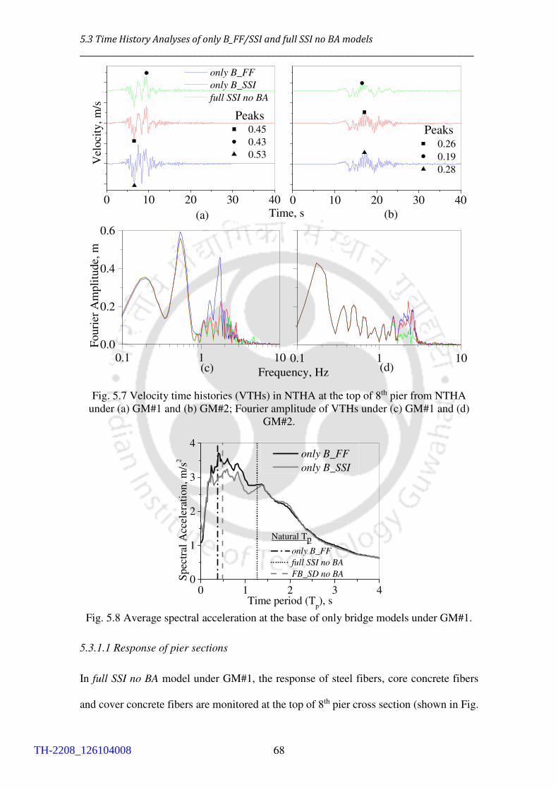
5.3 Time History Analyses of only B_FF/SSI and full SSI no BA models
______________________________________________________________________
68
0 10 20 30 40 0 10 20 30 40
Peaks 0.45
0.43
0.53
only B_FF only B_SSI full SSI no BA
Vel
oci
ty,
m/s
Time, s(a)
Peaks 0.26
0.19
0.28
(b)
Fig. 5.7 Velocity time histories (VTHs) in NTHA at the top of 8th pier from NTHA
under (a) GM#1 and (b) GM#2; Fourier amplitude of VTHs under (c) GM#1 and (d)
GM#2.
0 1 2 3 40
1
2
3
4
Natural Tp
only B_FF full SSI no BA FB_SD no BAS
pec
tral
Acc
eler
atio
n,
m/s
2
Time period (Tp), s
only B_FF only B_SSI
Fig. 5.8 Average spectral acceleration at the base of only bridge models under GM#1.
5.3.1.1 Response of pier sections
In full SSI no BA model under GM#1, the response of steel fibers, core concrete fibers
and cover concrete fibers are monitored at the top of 8th pier cross section (shown in Fig.
0.1 1 100.0
0.2
0.4
0.6
(d)(c)
Fouri
er A
mpli
tude,
m
Frequency, Hz
0.1 1 10
TH-2208_126104008

Seismic Analysis of RC Integral Bridge
______________________________________________________________________
69
3.1) and shown in Fig. 5.9. Stress–strain response in Steel fiber 1 (in Fig. 5.9(a)) is
nonlinear in tension and has yielded (with yield strength fy = 276 MPa), and forming
nonlinear excursions during dynamic analysis. In Fig. 5.9(b), the behaviour of Steel fiber
2 remains in linear elastic range under axial compression. Core concrete (Figs. 5.9(c) and
5.9(d)) fibers are linear elastic and have not reached the maximum compressive strength
of 34.5 MPa. Although the cover concrete fibers undergo cracking (Figs. 5.9(e) and
5.9(f)), the crushing of cover concrete is not observed. However, the cover concrete at
Cover Concrete fiber 1 undergoes nonlinear behaviour under GM#1 although the level of
nonlinearity is very small. Fibers have some residual response after the nonlinear dynamic
analysis. Residual response in each fiber depends on individual fiber’s nonlinearity that
has developed during the earthquake motion and on nonlinear deformation of under lying
foundation soil. The permanent deformation of soil domain can influence the residual
response of the bridge structure.
In Fig. 5.10, the moment-curvature response is shown at the top of the 8th pier and
base of the 1st pier during NTHA under GM#1 and GM#2. Under GM#1, the negative
moment-curvature are higher at the top (Fig. 5.10(a)) and positive moment-curvature are
higher at base (Fig. 5.10(c)) of pier cross-section, respectively. In Figs. 5.10(b) and
5.10(d) under GM#2, there is insignificant nonlinearity in structural members with very
less nonlinear excursions. At end of dynamic analysis, the residual responses under GM#2
is mainly due to gravity load analysis.
5.3.2 Response of soil
Figures 5.11(a) and 5.11(b) show the shear stress-shear strain response of soil elements
at location#1, at the depth of 7 m from soil surface in (Fig. 5.2) under GM#1 and GM#2,
respectively. In Fig. 5.11(a) extensive soil nonlinearity in observed with wider loops. In
Fig. 5.11(b,) one small loop has formed and the stress-strain variation range is quite low
TH-2208_126104008

5.3 Time History Analyses of only B_FF/SSI and full SSI no BA models
______________________________________________________________________
70
due to lower intensity of input motion. While at location#2 (in Fig. 5.11(c)), at the depth
of 34 m from soil surface, the loops are comparatively narrower than those formed at
location#1 because the soil element at higher depth gets more confined than the soil
element at shallow depth. Under GM#2, in Fig. 5.11(d), soil is linear elastic.
-100
0
100
200
300
(f)(e)
(d)(c)
(b)(a)
residual response
initial resposne
-8
-6
-4
-2
0
Str
ess,
MP
a
-0.2 -0.1 0.0 0.1 0.2-12
-10
-8
-6
-4
-2
0
Strain (%)
-0.2 -0.1 0.0 0.1 0.2
Fig. 5.9 Stress-strain response of fibers under GM#1 at top cross section of 8th pier: for
(a) Steel fiber 1, (b) Steel fiber 2, (c) Core Concrete fiber 1, (d) Core Concrete fiber 2
(e) Cover concrete fiber 1 and (f) Cover concrete fiber 2 for full SSI no BA model
TH-2208_126104008
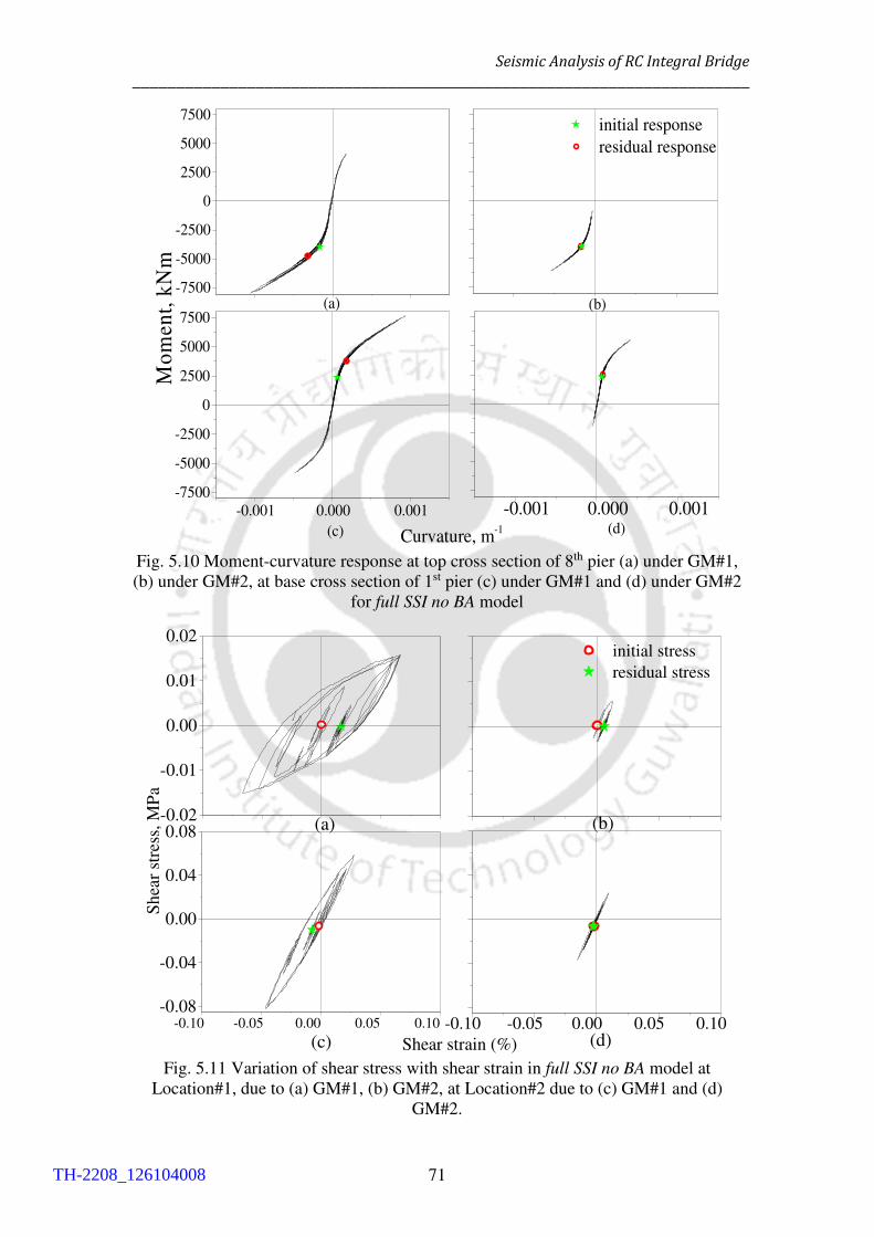
Seismic Analysis of RC Integral Bridge
______________________________________________________________________
71
-7500
-5000
-2500
0
2500
5000
7500
(d)(c)
(b)
Mo
men
t, k
Nm
(a)
initial response
residual response
-0.001 0.000 0.001
-7500
-5000
-2500
0
2500
5000
7500
Curvature, m-1
-0.001 0.000 0.001
Fig. 5.10 Moment-curvature response at top cross section of 8th pier (a) under GM#1,
(b) under GM#2, at base cross section of 1st pier (c) under GM#1 and (d) under GM#2
for full SSI no BA model
-0.02
-0.01
0.00
0.01
0.02
(d)(c)
(b)
Sh
ear
stre
ss,
MP
a
(a)
initial stress
residual stress
-0.10 -0.05 0.00 0.05 0.10-0.08
-0.04
0.00
0.04
0.08
Shear strain (%)
-0.10 -0.05 0.00 0.05 0.10
Fig. 5.11 Variation of shear stress with shear strain in full SSI no BA model at
Location#1, due to (a) GM#1, (b) GM#2, at Location#2 due to (c) GM#1 and (d)
GM#2.
TH-2208_126104008
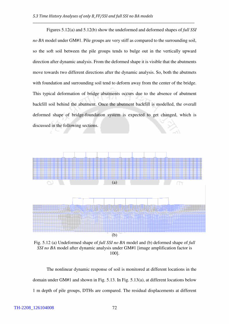
5.3 Time History Analyses of only B_FF/SSI and full SSI no BA models
______________________________________________________________________
72
Figures 5.12(a) and 5.12(b) show the undeformed and deformed shapes of full SSI
no BA model under GM#1. Pile groups are very stiff as compared to the surrounding soil,
so the soft soil between the pile groups tends to bulge out in the vertically upward
direction after dynamic analysis. From the deformed shape it is visible that the abutments
move towards two different directions after the dynamic analysis. So, both the abutmets
with foundation and surrounding soil tend to deform away from the center of the bridge.
This typical deformation of bridge abutments occurs due to the absence of abutment
backfill soil behind the abutment. Once the abutment backfill is modelled, the overall
deformed shape of bridge-foundation system is expected to get changed, which is
discussed in the following sections.
(a)
(b)
Fig. 5.12 (a) Undeformed shape of full SSI no BA model and (b) deformed shape of full SSI no BA model after dynamic analysis under GM#1 [image amplification factor is
100].
The nonlinear dynamic response of soil is monitored at different locations in the
domain under GM#1 and shown in Fig. 5.13. In Fig. 5.13(a), at different locations below
1 m depth of pile groups, DTHs are compared. The residual displacements at different
TH-2208_126104008

Seismic Analysis of RC Integral Bridge
______________________________________________________________________
73
locations are observed to vary because of different extents of soil nonlinearity at different
locations of the soil domain. At a depth of 1 m below the bottom of abutment piles, soil
gets displaced in two different directions (Fig. 5.12(b)). The minimum residual response
is observed below 1 m depth of left pile group due to development of lesser nonlinearty
in the soil elements as compared to the other two monitored locations. In Fig. 5.13(b),
DTHs at the boundary (far field zone) of soil domain are quite similar between the full
SSI no BA and the free field soil domain models due to similarity of energy dissipation
mechanisms. The soil boundary of full SSI no BA model is far enough from near field
excited zone of bridge which is unable to radiate any spurious waves back into the excited
zone of soil domian, so the boundary behaves like a free field soil column.
0 10 20 30 40-0.15
-0.10
-0.05
0.00
0.05
0.10
0.15
below left pg
below 5th pg
below right pg
(b)
Dis
pla
cem
ent,
m
Time, s(a)0 10 20 30 40
full SSI no BA Free Field
Fig. 5.13 Comparison of horizontal DTHs in soil domain at (a) different locations below
the bridge and (b) near the boundaries in free field soil domain and full SSI no BA
models under GM#1 (‘pg’ stands for pile group).
In Figs. 5.14(a) and 5.14(b), the maximum acceleration profiles are shown for
nonlinear free field soil domain model along with the response of full SSI no BA model
under linear and nonlinear behaviours at the monitored soil column (Fig. 5.2) under
GM#1 and GM#2, respectively. For the GM#1, linear full SSI no BA model shows higher
response in terms of both acceleration and strain parameters. In peak acceleration profile
obtained for nonlinear behaviour under GM#1 (Fig. 5.14(a)), the peak acceleration
TH-2208_126104008

5.3 Time History Analyses of only B_FF/SSI and full SSI no BA models
______________________________________________________________________
74
increases upto a depth of 25 m then decreases upto 75 m and after that it slightly increases
till the bottom of the column. But for linear behaviour of the same model, the peak
acceleration decreases from the soil surface to the depth of 35 m then increases upto 50
m of depth followed by decreasing acceleration upto 120 m depth; finally, the profile
becomes similar for both the behaviours. For nonlinear behaviour of the full SSI no BA
model, the peak acceleration near the soil surface reduces as the pile groups are acting as
binding elements at foundation soil layer. In linear soil domain, due to seismic wave’s
amplification, the peak acceleration increases near the soil surface. But for nonlinear
cases, peak acceleration depends on the nonlinearity of soil; due to nonlinearity of soil
elements acceleration gets reduced. Under GM#2, soil nonlinearity is effective upto 25 m
depth from the soil surface. Below that depth, the peak response for the linear and the
nonlinear behaviours of the full SSI no BA model and free field soil model are almost
same due to insignificant nonlinearity developed in soil domain.
The observed peak shear strain profiles at the monitored soil column under GM#1
and GM#2 are shown in Figs. 5.14(c) and 5.14(d), respectively. The peak shear strains of
the full SSI no BA models under linear and nonlinear behaviours increase upto 20 m depth
then decreases till a depth of 70 m. Seismic waves amplified at the soil surface from bed
rock level and the nonlinearity of soil is found to be maximum in the ground level. Thus,
this results in higher shear strain upto a certain depth of 20 m from the soil surface in both
linear and nonlinear soil domains. Beyond that depth, the peak strain profile remains
almost constant for both the models. Peak strain of free field nonlinear soil model is less
at the depth of 20 m then it starts to increase leading to similar profile trends. Under
GM#2, strain profiles vary in terms of strain upto a depth of 30 m, then follow similar
profile trends as obtained under GM#1. Peak shear strain increases in SP/SM soil layers
as in this layer, the soil undrained shear strength of the soil is considerably low. For linear
TH-2208_126104008

Seismic Analysis of RC Integral Bridge
______________________________________________________________________
75
behaviour of full SSI no BA model, higher peak acceleration causes reduction in peak
shear strain. For nonlinear behaviour of the same model, the peak shear strain also
increases with the peak acceleration. Peak acceleration and shear strain both are found to
be significantly higher in silty sand (SP/SM) than other soil layers because of its
considerably lower undrained shear strength than the top and bottom layers.
5.3.3 Response of full SSI no BA model across depth
During NTHA, the observed variation of horizontal acceleration at different points along
the vertical line of right abutment pile-group of full SSI no BA model is shown in Figure
5.15. As the nonlinearity of soil is higher below the right abutment pile group as compared
to the other locations in the soil domain (Fig. 5.13(a)), the ATHs are obtained at right
abutment-deck joint, base of right abutment and below the right abutment pile group
under GM#1 and GM#2 (Figs. 5.15(a) and 5.15(b)). Under GM#1, the ATH gets
amplified from 1 m depth below the pile group to the bottom of the abutment and further
up to the deck level. Under the GM#2, amplification of ATH at deck level is also
observed. Under GM#2, the variation of horizontal acceleration also shows similar trend
at all the monitored locations. From the normalized Fourier amplitude of ATHs under
GM#1 in Fig. 5.15(c), significant deck amplification is visible in the range of 1–10 Hz of
frequency. Whereas, at base of the abutment and below the pile group nodes contain
similar Fourier amplitude upto 5 Hz. Beyond 5 Hz of frequency, the base of the abutment
motion contains marginally higher acceleration. Under GM#2, motion at deck gets
amplified beyond 1 Hz of frequency as compared to the other two locations. Below the
pile group, acceleration response is minimum because linear elastic pile foundation has a
restraining effect on the foundation soil. At deck level, maximum amplification of the
response occurs due to the absence of abutment backfill soil which would have offered
some restraint at both the ends of the bridge in the longitudinal direction.
TH-2208_126104008
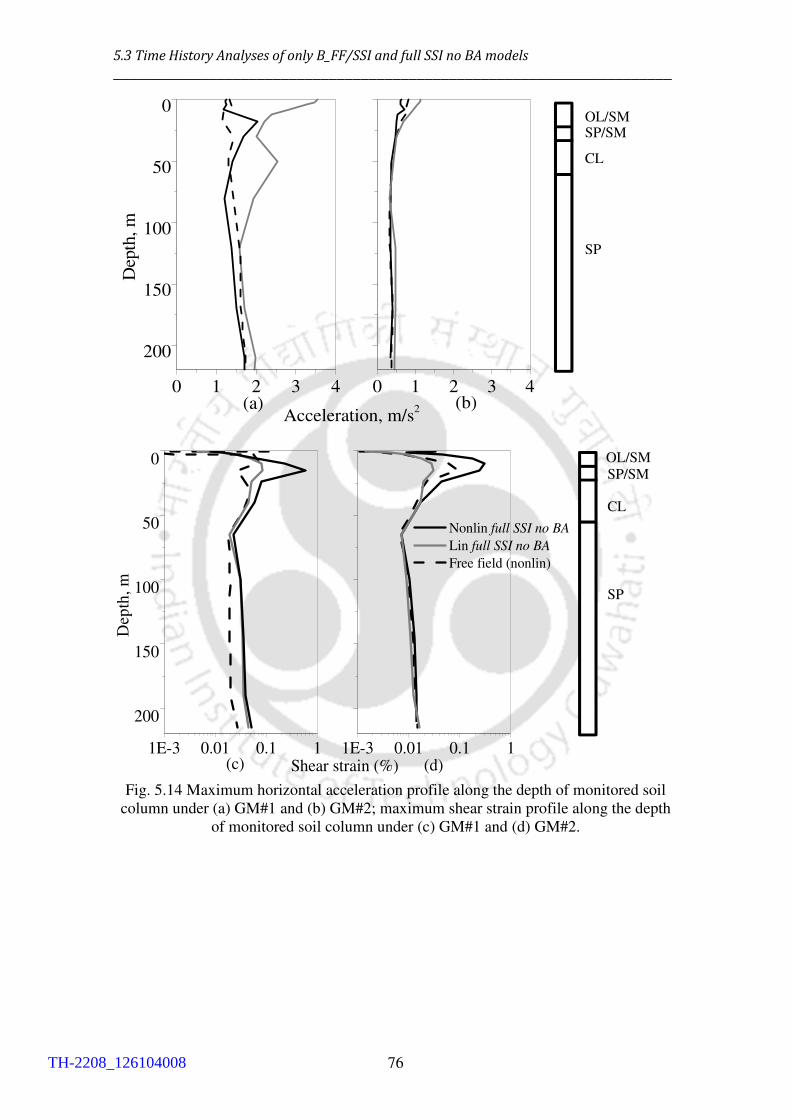
5.3 Time History Analyses of only B_FF/SSI and full SSI no BA models
______________________________________________________________________
76
0 1 2 3 4
200
150
100
50
0
(b)
Dep
th, m
Acceleration, m/s2(a)
0 1 2 3 4
1E-3 0.01 0.1 1
200
150
100
50
0
Dep
th,
m
Shear strain (%) 1E-3 0.01 0.1 1
(d)
Nonlin full SSI no BA Lin full SSI no BA Free field (nonlin)
(c)
Fig. 5.14 Maximum horizontal acceleration profile along the depth of monitored soil
column under (a) GM#1 and (b) GM#2; maximum shear strain profile along the depth
of monitored soil column under (c) GM#1 and (d) GM#2.
OL/SM
SP/SM
CL
SP
OL/SM SP/SM
CL
SP
TH-2208_126104008

Seismic Analysis of RC Integral Bridge
______________________________________________________________________
77
0 10 20 30 40-4
-2
0
2
4
Time, s
Peaks
deck accel. at 9.54s, 3.255
abutment bottom accel. at 9.805s,1.29
below pg accel. at 6.26s, 1.09
(d)(c)
(b)
deck response
base of abutment
below pile group
Acc
eler
atio
n,
m/s
2
(a)0 10 20 30 40
0.1 1 100
1
2
Fo
uri
er A
mp
litu
de,
m/s
Frequency, Hz
0.1 1 10
Fig. 5.15 Recorded ATHs along the vertical profile of right abutment-pile group-
foundation (a) under GM#1, (b) under GM#2; FTs of ATHs (c) under GM#1 and (d)
under GM#2 in full SSI no BA model.
5.4 Complementary Investigation of Material Properties in Full SSI No BA Model
The response of bridge-foundation-soil system with linear and nonlinear behaviours of
different components are discussed in this section, i.e., linear behaviour of bridge with
nonlinear behaviour of soil (lin str+nl soil no BA) model and nonlinear behaviour of
bridge with linear behaviour of soil (nl str+lin soil no BA) model. The intention of the
study is to investigate the individual effect of material nonlinearity on the overall response
of the bridge. Under low level of shaking, nl str+lin soil no BA model remains linear like
linear full SSI no BA model. Lin str+nl soil no BA model can be taken as an example of
very stiff structure with very flexible soil profile e.g., nuclear structure. Although the vice
versa is not realistic physically, still to investigate the influence of nonlinear structure on
linear soil domain this case has been considered for the study.
TH-2208_126104008

5.4 Complementary Investigation of Material Properties in Full SSI No BA Model
______________________________________________________________________
78
5.4.1 Linear structural behaviour
For linear behaviour of the superstructure and the substructure, the influence of soil
nonlinearity is visible by comparing the response of the linear behaviour of full SSI no
BA model with the response of lin str+nl soil no BA model. From the observed SFTHs
shown in Figs. 5.16(a) and 5.16(b), the nonlinearity of soil dominates the response in high
intensity of shaking under GM#1for the lin str+nl soil no BA model. The peak shear force
at the top of 8th pier gets reduced by a factor of 2.9 from the linear behaviour of full SSI
no BA model to the response of lin str+nl soil no BA model. Normalized Fourier spectra
of SFTHs are shown in Figs.5.16(c) and 5.16(d) under GM#1 and GM#2, respectively.
From the Fig.5.16(c), it is observed that under GM#1, the shear force content is higher in
frequency domain as compared to the content obtained under GM#2. Once the soil is
nonlinear, the peaks of SFTHs occur at different frequencies in these two models. To
study the shift in the frequency corresponding to the occurrence of peak Fourier
amplitude, normalized FTs are studied. From the normalized response spectra plot in Fig.
5.16(c), it is visible that peaks of Fourier amplitudes are occurring at the frequency of
2.25Hz and 2.38Hz for the linear behaviour of full SSI no BA model and lin str+nl soil
no BA model, respectively. Due to nonlinearity of soil domain, the latter model is more
deformable and comparatively less seismic forces are imposed at the base of bridge
substructure. Due to linear elastic material behaviour, the bridge structure is stiffer under
this condition and leads to the mentioned shift in frequency. In Fig. 5.16(d), FTs of SFTHs
of Fig. 5.16(b) are plotted and normalized by the peak amplitude value obtained from FT
under GM#2 for the linear behaviour of full SSI no BA model to emphasize on the
nonlinearity developed in lin str+nl soil no BA model under both the ground motions.
The overall response for both the models gets reduced due to low intensity of shaking
under GM#2, thus, the difference in the FT curves is not that significant.
TH-2208_126104008

Seismic Analysis of RC Integral Bridge
______________________________________________________________________
79
0 10 20 30 40-4000
-2000
0
2000
4000
(b)
Peak (1934, 9.34s)
Peak (3661, 6.44s)S
hea
r F
orc
e, k
N
Time, s(a)0 10 20 30 40
Peak (15.995s, 1733)
Peak (15.615s, 1219)
Linear full SSI no BA lin str+nl soil no BA
0.1 1 100.0
0.2
0.4
0.6
0.8
1.0
0.1 1 10
No
rmal
ized
Fo
uri
er A
mpli
tude
(d)Frequency, Hz(c)
Fig.5.16 Comparison of SFTHs at the top of 8th pier of bridge for linear behaviour of
full SSI no BA model and lin str+nl soil no BA model under (a) GM# 1, (b) GM#2 and
normalized FTs of (c) SFTHs shown in (a) and (d) SFTHs shown in (b).
The same trend, as noted for the SFTHs, is observed in the velocity time history
at the deck level for the two models under GM#1 and GM#2 (Figs. 5.17(a) and 5.17(b)).
The observed peak velocities are 0.71 m/s and 0.40 m/s for the linear behaviour of full
SSI no BA model and lin str+nl soil no BA model, respectively. Under GM#2, the overall
response gets reduced which leads to very small difference in the VTHs of the two
models. However, both the normalized FT plots show a significant frequency shift in the
occurrence of peak Fourier amplitude of VTHs (Figs. 5.17(c) and 5.17(d)). Even for the
VTH under GM#2, the difference in the distribution of deck velocity response in
frequency domain is very obvious for the two models, unlike the FTs of SFTHs where
the difference was very small.
TH-2208_126104008
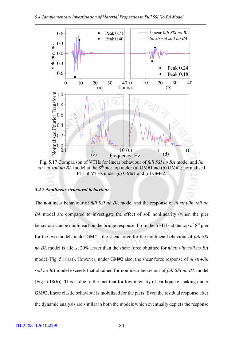
5.4 Complementary Investigation of Material Properties in Full SSI No BA Model
______________________________________________________________________
80
0 10 20 30 40
-0.6
-0.3
0.0
0.3
0.6 Peak 0.71
Peak 0.40
Vel
oci
ty, m
/s
0 10 20 30 40
Peak 0.24
Peak 0.18
Linear full SSI no BA lin str+nl soil no BA
(b)Time, s(a)
0.1 1 100.0
0.2
0.4
0.6
0.8
1.0
No
rmali
sed
Fo
uri
er T
ran
sfo
rm
0.1 1 10(d)Frequency, Hz(c)
Fig. 5.17 Comparison of VTHs for linear behaviour of full SSI no BA model and lin
str+nl soil no BA model at the 8th pier top under (a) GM#1and (b) GM#2; normalised
FTs of VTHs under (c) GM#1 and (d) GM#2.
5.4.2 Nonlinear structural behaviour
The nonlinear behaviour of full SSI no BA model and the response of nl str+lin soil no
BA model are compared to investigate the effect of soil nonlinearity (when the pier
behaviour can be nonlinear) on the bridge response. From the SFTHs at the top of 8th pier
for the two models under GM#1, the shear force for the nonlinear behaviour of full SSI
no BA model is atleast 20% lesser than the shear force obtained for nl str+lin soil no BA
model (Fig. 5.18(a)). However, under GM#2 also, the shear force response of nl str+lin
soil no BA model exceeds that obtained for nonlinear behaviour of full SSI no BA model
(Fig. 5.18(b)). This is due to the fact that for low intensity of earthquake shaking under
GM#2, linear elastic behaviour is mobilized for the piers. Even the residual response after
the dynamic analysis are similar in both the models which eventually depicts the response
TH-2208_126104008

Seismic Analysis of RC Integral Bridge
______________________________________________________________________
81
under the initial static gravity analysis. So, in the modelling of this specific soil-
foundation-bridge system, under higher PGA (≥ 0.48g of base excitation) nonlinearity of
structure is likely to govern the response.
As observed in the results of the previous section, the normalized FT plots of
SFTHs for the models show the same trend in the shift of frequency for the occurrence of
peak Fourier amplitude under GM#1 (Fig. 5.18(c)). The peaks of normalized Fourier
amplitude occur at 1.2 Hz and 0.6 Hz for nl str+lin soil no BA and nonlinear behaviour
of full SSI no BA model, respectively. Under GM#2, the peaks of the Fourier amplitudes
occur at 2.27 Hz and 2.34 Hz, respectively, for the two models (Fig. 5.18(d)). Due to high
energy content in linear soil domain, nl str+lin soil no BA model’s Fourier amplitude is
significantly higher than the other one (Fig. 5.18(c)). For the nonlinear behaviour of full
SSI no BA model, the input seismic energy gets reduced through soil damping around the
bridge foundation; this further reduces the possibility of nonlinear behaviour in the bridge
piers. Hence, for that model, the bridge behaviour is comparatively stiffer as compared to
the behaviour obtained for nl str+linsoil no BA model. From the velocity time histories
at right abutment-deck junction, the peak velocities occur at 8.885 s and 9.495s under
GM#1 and at 17.065 s and 16.525 s under GM#2 for nl str+lin soil no BA model and for
nonlinear behaviour of full SSI no BA model, respectively (Figs. 5.19(a) and 5.19(b)).
Due to nonlinearity of soil, the peak velocity response of bridge reduces significantly
under both the ground motions for the nonlinear behaviour of full SSI no BA model. Under
both the ground motions, the frequency for the occurrence of peak Fourier amplitude is
observed to be higher for the nl str+lin soil no BA model as compared to the other model
(Figs. 5.19(c) and 5.19(d)). The difference in the magnitude of the peak Fourier
amplitudes for the models also reflects the higher velocity response of the nl str+lin soil
no BA model as compared to the other model. From these type of comparisons, it is easy
TH-2208_126104008

______________________________________________________________________
82
to conclude that under low intensity of ground motion, nonlinearity of soil highly
influences the nonlinear behaviour of structure.
0 10 20 30 40-2000
-1000
0
1000
2000
(b)
Peak (8.475, 1642.7)
Peak (9.405, 1300.4)
Sh
ear
Fo
rce,
kN
Time, s(a)
0 10 20 30 40
Peak (1259, 16.96s)
Peak (966, 16.43s)
nl str+lin soil no BA Nonlinear full SSI no BA
0.1 1 100.0
0.2
0.4
0.6
0.8
1.0
0.1 1 10(d)
Norm
alis
ed F
ouri
er T
ransf
orm
(c)Frequency, Hz
Fig. 5.18 Comparison of SFTHs for the nonlinear behaviour of full SSI no BA model
and the nl str+lin soil no BA model at the top of 8th pier of bridge under (a) GM# 1 and
(b) GM#2; normalized FTs of SFTHs under (c) GM#1and (d) GM#2.
5.5 Influence of Abutment Backfill Interaction
After studying different modelling cases without abutment backfill interaction, finally
abutment backfill soil is modelled with four noded quadrilateral elements having pressure
independent multi-yield material properties. Nonlinear material properties of the backfill
soil are kept the same as that of the top surface soil layer. Abutment and backfill interface
nodes are connected with equal degrees of freedom in horizontal and vertical directions
in the 2D plain strain model. The soil-foundation-bridge system with abutment backfill
soil is referred to as full SSI with BA model in the further study. The undeformed and
deformed shapes of the full SSI with BA model in the near field zone are shown in Figs.
TH-2208_126104008
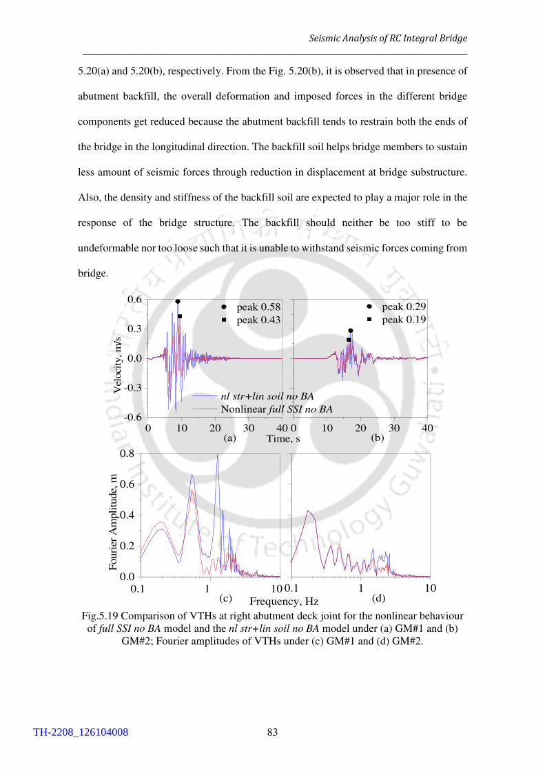
Seismic Analysis of RC Integral Bridge
______________________________________________________________________
83
5.20(a) and 5.20(b), respectively. From the Fig. 5.20(b), it is observed that in presence of
abutment backfill, the overall deformation and imposed forces in the different bridge
components get reduced because the abutment backfill tends to restrain both the ends of
the bridge in the longitudinal direction. The backfill soil helps bridge members to sustain
less amount of seismic forces through reduction in displacement at bridge substructure.
Also, the density and stiffness of the backfill soil are expected to play a major role in the
response of the bridge structure. The backfill should neither be too stiff to be
undeformable nor too loose such that it is unable to withstand seismic forces coming from
bridge.
0 10 20 30 40-0.6
-0.3
0.0
0.3
0.6peak 0.58
peak 0.43
(b)
Vel
oci
ty, m
/s
Time, s(a)0 10 20 30 40
peak 0.29
peak 0.19
nl str+lin soil no BA Nonlinear full SSI no BA
0.1 1 100.0
0.2
0.4
0.6
0.8
(d)
Fouri
er A
mpli
tude,
m
Frequency, Hz(c)0.1 1 10
Fig.5.19 Comparison of VTHs at right abutment deck joint for the nonlinear behaviour
of full SSI no BA model and the nl str+lin soil no BA model under (a) GM#1 and (b)
GM#2; Fourier amplitudes of VTHs under (c) GM#1 and (d) GM#2.
TH-2208_126104008

5.5 Influence of Abutment Backfill Interaction
______________________________________________________________________
84
(a)
(b)
Fig.5.20 (a) Undeformed shape and (b) deformed shape of full SSI with BA model after
dynamic analysis under GM#1.
SFTHs are plotted at the top of 8th pier in Fig. 5.21(a) for full SSI no/with BA models
under GM#1. Peak SF at the top of 8th pier is atleast 31% lower in full SSI with BA model
as compared to the other one. From the residual shear force at the end of GM#1, it can be
stated that due to abutment backfill interaction the residual force at the top of the 8th pier
is 133 kN; whereas, in full SSI no BA model, the residual SF is 709 kN. Thus, the sructure
is going through significant nonlinearity at the end of dynamic motion for the full SSI no
BA model. From the normalised fourier amplitude of SFTHs in Fig. 5.21(b), full SSI no
BA model’s peak Fourier amplitude is higher than full SSI with BA model as it carries
more seismic forces. With backfill soil, the abutments and the superstructure (deck)
undergo less amount of deformation because the seismic forces dissipate through backfill
and it results in significant backfill deformation by the end of dynamic analysis
(Fig.5.20(b)). At a depth of 1 m below the tip of pile foundation underneath the 8th pier,
Location #3
TH-2208_126104008

Seismic Analysis of RC Integral Bridge
______________________________________________________________________
85
displacement time histories (DTHs) are shown for both the models (Fig. 5.21(c)) and in
full SSI with BA model, foundation soil is more deformable than the other one. The peak
acceleration at the top of 8th pier reduces from 2.98 m/s2 to 1.94 m/s2in full SSI with BA
model (Fig. 5.21(d)). Hence, seismic acceleration of the bridge stricture in full SSI with
BA model is less than full SSI no BA model under GM#1, which reduces the overall deck
response. At location#3, free field soil has a peak displacement of 0.15 m. The full SSI
with BA model and the free field soil domain have a relative displacement of 0.02 m after
the instant of peak response and relative residual displacement is also 0.027 m which is
insufficient to mobilize the passive pressure under dynamic loading. According to
AASHTO (2012), integral abutment should be allowed to get displaced upto maximum
limit of 0.091 m under cyclic loading.
In Fig. 5.22, SFTHs are monitored at the top of 8th pier under GM#2. The abutment
backfill soil influences the response of structure as well as soil in case of low intensity of
input motion too. In presence of abutment backfill, the peak shear force at the top of 8th
pier reduces from 966.4kN to 805.8kN. The normalised Fourier amplitudes have been
obtained by normalising the FT values with respect to peak amplitude of full SSI no BA
model. In normalised fourier amplitude of SFTHs (Fig. 5.22(b)), the differences in
Fourier amplitude for the frequency range of 1–4 Hz occur because full SSI no BA model
carries higher seismic forces in that frequency range. In Fig. 5.22(c), ATHs are shown at
left deck-abutment joint and the peaks of ATHs are 1.26 m/s2 and 1.35 m/s2 for full SSI
with BA and full SSI no BA model, respectively. Fig. 5.22(d) shows fourier amplitude of
ATHs shown in Fig. 5.22(c). The peaks of fourier amplitudes occur in the frequency range
of 2.5 Hz to 3.3 Hz for the models.
TH-2208_126104008
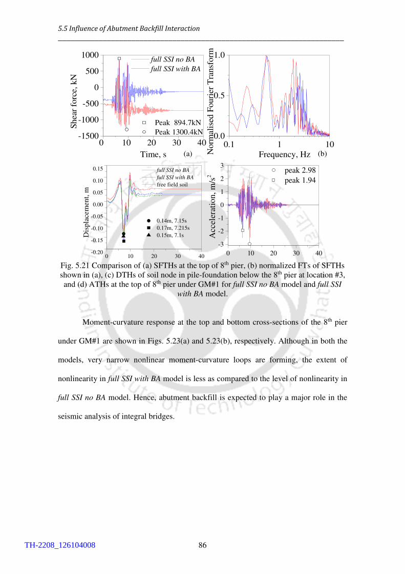
5.5 Influence of Abutment Backfill Interaction
______________________________________________________________________
86
0 10 20 30 40-1500
-1000
-500
0
500
1000
(b)
Peak 894.7kN
Peak 1300.4kN
Shea
r fo
rce,
kN
Time, s
0.1 1 100.0
0.5
1.0 full SSI no BA full SSI with BA
Norm
alis
ed F
ouri
er T
ransf
orm
Frequency, Hz(a)
0 10 20 30 40-0.20
-0.15
-0.10
-0.05
0.00
0.05
0.10
0.15 full SSI no BA full SSI with BA free field soil
0.14m, 7.15s
0.17m, 7.215s
0.15m, 7.1sDis
pla
cem
ent,
m
0 10 20 30 40
-3
-2
-1
0
1
2
3 peak 2.98
peak 1.94
Acc
eler
atio
n,
m/s
2
Fig. 5.21 Comparison of (a) SFTHs at the top of 8th pier, (b) normalized FTs of SFTHs
shown in (a), (c) DTHs of soil node in pile-foundation below the 8th pier at location #3,
and (d) ATHs at the top of 8th pier under GM#1 for full SSI no BA model and full SSI with BA model.
Moment-curvature response at the top and bottom cross-sections of the 8th pier
under GM#1 are shown in Figs. 5.23(a) and 5.23(b), respectively. Although in both the
models, very narrow nonlinear moment-curvature loops are forming, the extent of
nonlinearity in full SSI with BA model is less as compared to the level of nonlinearity in
full SSI no BA model. Hence, abutment backfill is expected to play a major role in the
seismic analysis of integral bridges.
TH-2208_126104008

Seismic Analysis of RC Integral Bridge
______________________________________________________________________
87
0 10 20 30 40
-900
-600
-300
0
300Peak 966.4kN
Peak 805.8kNS
hea
r F
orc
e, k
N
Time, s
0.1 1 101E-3
0.01
0.1
1
(b)
full SSI no BA
full SSI with BA
No
rmal
ised
Fo
uri
er T
ran
sfo
rm
Frequency, Hz(a)
0 10 20 30 40-1.5
-1.0
-0.5
0.0
0.5
1.0
1.5 Peak 1.26
Peak 1.35
Acc
eler
atio
n, m
/s2
Time, s0.1 1 10
0.0
0.5
1.0
1.5
(c) Frequency, Hz
Fouri
er A
mp
litu
de,
m/s
(d)
Fig. 5.22 Comparison of (a) SFTHs at the top of 8th pier, (b) normalized FTs of SFTHs
shown in (a) in log-log scale, (c) ATHs at 1st pier top, (d) FTs of ATHs shown in (c)
under GM#2 for full SSI no BA model and full SSI with BA model.
-0.002 -0.001 0.000 0.001 0.002-10.0k
-5.0k
0.0
5.0k
10.0kresidual response
residual response
full SSI with BA full SSI no BA
(b)Curvature, m-1
Mo
men
t, k
Nm
(a)-0.002 -0.001 0.000 0.001 0.002
Fig. 5.23 Comparison of moment curvature response at the (a) bottom and (b) top cross-
sections of the 8th pier under GM#1 for full SSI no BA model and full SSI with BA
model.
TH-2208_126104008
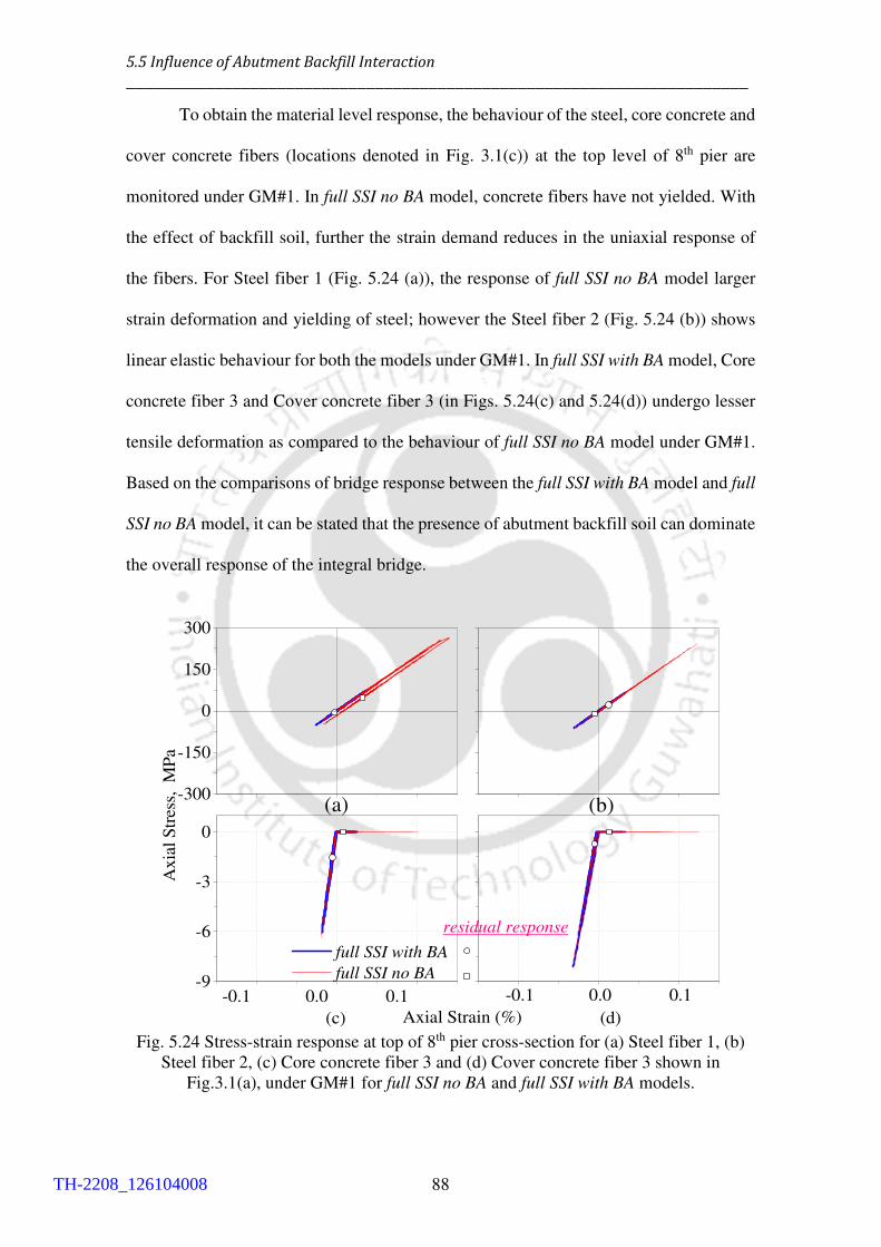
5.5 Influence of Abutment Backfill Interaction
______________________________________________________________________
88
To obtain the material level response, the behaviour of the steel, core concrete and
cover concrete fibers (locations denoted in Fig. 3.1(c)) at the top level of 8th pier are
monitored under GM#1. In full SSI no BA model, concrete fibers have not yielded. With
the effect of backfill soil, further the strain demand reduces in the uniaxial response of
the fibers. For Steel fiber 1 (Fig. 5.24 (a)), the response of full SSI no BA model larger
strain deformation and yielding of steel; however the Steel fiber 2 (Fig. 5.24 (b)) shows
linear elastic behaviour for both the models under GM#1. In full SSI with BA model, Core
concrete fiber 3 and Cover concrete fiber 3 (in Figs. 5.24(c) and 5.24(d)) undergo lesser
tensile deformation as compared to the behaviour of full SSI no BA model under GM#1.
Based on the comparisons of bridge response between the full SSI with BA model and full
SSI no BA model, it can be stated that the presence of abutment backfill soil can dominate
the overall response of the integral bridge.
-300
-150
0
150
300
(b)
full SSI with BA full SSI no BA
Axia
l S
tres
s, M
Pa
(a)
residual response
-0.1 0.0 0.1
-9
-6
-3
0
(d)(c) Axial Strain (%)
-0.1 0.0 0.1
Fig. 5.24 Stress-strain response at top of 8th pier cross-section for (a) Steel fiber 1, (b)
Steel fiber 2, (c) Core concrete fiber 3 and (d) Cover concrete fiber 3 shown in
Fig.3.1(a), under GM#1 for full SSI no BA and full SSI with BA models.
TH-2208_126104008

Seismic Analysis of RC Integral Bridge
______________________________________________________________________
89
5.6 Introduction of Nonlinear Spring-Dashpot Model
Analysis of SSI problems with detailed modelling of soil domain involves significant
computational efforts. In order to reduce that effort, simplified modelling using spring-
dashpot elements is adopted as an alternative method. Hence, nonlinear springs and
dashpots are introduced to represent soil stiffness, replicating Soil-Pile Interaction (SPI)
and Abutment Backfill Interaction (ABI) in bridge with spring dashpot model without
abutment backfill soil (referred to as FB_SD no BA model) and in bridge with spring
dashpot model with abutment backfill soil (referred as FB_SD with BA model). In this
section, structural response are determined using nonlinear time history analysis, to
investigate the overall seismic response of the integral bridge using both detailed domain
modelling approach and spring-dashpot modelling approach of the soil.
5.6.1 Comparison between full SSI no BA and FB_SD no BA models
Under GM#1, the ATHs at the top and the bottom of the 8th pier are shown in Figs. 5.25(a)
and 5.25(b). The respective Fourier Transforms (FT) are shown in the Figs. 5.25(c) and
5.25(d). The ATHs at the bottom of the pier match closely with each other (Figs. 5.25(a)
and 5.25(c)), but at the deck level (Figs. 5.25(b) and 5.25(d)), FB_SD no BA model shows
more amplified response as compared to the full SSI no BA model. However, the peaks
of Fourier amplitude occur at 1.78 Hz and 2.29 Hz for FB_SD no BA and full SSI no BA
models, respectively. Foundation of FB_SD no BA model is observed to be stiffer as the
API curves overestimate the lateral soil stiffness at different depths of the piles. Thus,
nonlinearity is unable to develop in the underlying soil. Moreover, an amplifying effect
is also noted at 1.78 Hz as the natural frequency of the model is 2.05 Hz, which is not
present in the full SSI no BA model.
TH-2208_126104008

5.6 Introduction of Nonlinear Spring-Dashpot Model
______________________________________________________________________
90
0 10 20 30 40-3
-2
-1
0
1
2
(c) (d)
Time, s
SB_SD no BA
full SSI no BA
Acc
eler
atio
n, m
/s2
0 10 20 30 40
0.1 1 100
1
2
3
4
Fou
rier
Am
pli
tude,
m/s
0.1 1 10
(b)
Frequency, Hz
(a)
Fig. 5.25 Comparison of ATHs for full SSI no BA model and FB_SD no BA model
under GM#1 at (a) the bottom and (b) the top of the 8th pier; (c) FT of the ATHs shown
in (a) and (d) FT of the ATHs in (b).
Similar response is observed for SFTHs shown in Fig. 5.26(a). Due to
amplification of seismic waves at the deck level, the peak shear force is higher in FB_SD
no BA model as compared to the full SSI no BA model. From the SFTH, it can be stated
that FB_SD no BA model carries significantly more seismic forces as compared to the full
SSI no BA model. Normalized FTs of the SFTHs are shown in Fig. 5.26(b) and the
magnitude of Fourier amplitude is significantly higher in FB_SD no BA model than full
SSI no BA model. The same behavior is also reflected from the moment-curvature
response at the top and bottom cross-sections of the 8th pier (Figs. 5.26(c) and 5.26(d)).
Moment-curvature response at the top of 8th pier is found to be lesser in FB_SD no BA
model and mainly forms negative moment-curvature loops in the third quadrant. At the
base of the 8th pier, moment curvature response (Fig. 5.26(d)) shows similar pattern on
the opposite quadrants. Thus, it can be stated that the response of the FB_SD no BA model
gets more amplified from the foundation to the deck level as compared to the full SSI no
TH-2208_126104008

Seismic Analysis of RC Integral Bridge
______________________________________________________________________
91
BA model. In conventional bridges, piers at the bottom sections are more prone to form
hinges. But in an integral bridge, in absence of any bearing and energy dissipating device,
top section of the pier can also attract high forces and moments, thus, making it prone to
formation of plastic hinges and subsequent failure.
0 10 20 30 40
-1500
-1000
-500
0
500
1000
1500
Peak
1300.4 kN
1485.3 kN
FB_SD no BA full SSI no BA
Shea
r F
orc
e, k
N
Time, s0.1 1 10
0.0
0.2
0.4
0.6
0.8
1.0
(b) Frequency, Hz
Norm
aliz
ed F
ouri
er A
mpli
tude
(a)
-0.004 -0.002 0.000 0.002 0.004-10.0k
-5.0k
0.0
5.0k
10.0k
Curvature, m-1
residual FB_SD no BA residual full SSI no BA
(d)
Mom
ent,
kN
m
(c)-0.004 -0.002 0.000 0.002 0.004
Fig. 5.26 Comparison of (a) Shear Force time history at the top of 8th pier and (b)
normalised FTs of the SFTHs for the full SSI no BA model and FB_SD no BA model;
moment-curvature response at the (c) top and (d) bottom cross-sections of the of 8th pier
under GM#1.
Under GM#2, SFTHs at the top of 8th pier (deck level) are shown for the two
models in Fig. 5.27(a). The difference in energy content of the response is observed
through the normalized FT of SFTHs in Fig. 5.27(b). Similar response is also obtained
under GM#2.
TH-2208_126104008

5.6 Introduction of Nonlinear Spring-Dashpot Model
______________________________________________________________________
92
0 10 20 30 40-1500
-1000
-500
0
500
1000
Peak
1266 kN
966 kN
FB_SD no BA full SSI no BA
Sh
ear
Fo
rce,
kN
Time, s
0.1 1 100.0
0.2
0.4
0.6
0.8
1.0
(b) Frequency, Hz
No
rmal
ised
Fo
uri
er T
ran
sfo
rm
(a)
Fig. 5.27 (a) SFTH at the top of 8th pier and (b) normalised FTs of the SFTHs in (a)
under GM#2.
5.6.2 Comparison between full SSI with BA and FB_SD with BA models
For comparison, the ATHs under GM#1 are shown at the bottom and the top of the eighth
pier in Figs. 5.28(a) and 5.28(b), and the corresponding Fourier amplitudes of ATHs are
shown in Figs. 5.28(c) and 5.28(d). Peak acceleration at the base of the pier in FB_SD
with BA model is marginally higher than that obtained for full SSI with BA model. Thus,
in Fig. 5.28(c), the Fourier amplitude is almost incomparable in frequency domain.
However, at the top of 8th pier (Fig. 5.28(b)), ATHs are quite comparable for both the
models. In Fig. 5.28(d), the peak Fourier amplitudes for FB_SD with BA and full SSI with
BA models are at 2.83Hz and 2.12Hz, respectively, which indicates that FB_SD with BA
model contains marginally higher seismic acceleration as compared to the full SSI with
BA model. Hence, the possibility of nonlinear behaviour is likely to be higher for FB_SD
with BA model.
TH-2208_126104008

Seismic Analysis of RC Integral Bridge
______________________________________________________________________
93
0 10 20 30 40
-2
-1
0
1
FB_SD with BA full SSI with BA
Time, s
Acc
eler
atio
n, m
/s2
0 10 20 30 40
(c) (d)
(a) (b)
0.1 1 100.0
0.5
1.0
1.5
2.0
Fouri
er A
mpli
tude,
m/s
0.1 1 10
Frequency, Hz Fig. 5.28 Comparison of ATHs for full SSI with BA model and FB_SD with BA model at
the (a) top and the (b) bottom of 8th pier; (c) Fourier transform of the ATHs shown at
the (a) bottom and (d) the top of 8th pier under GM#1.
Under GM#2, similar responses are observed for the ATHs at the bottom and top
of first pier (Figs. 5.29(a) and 5.29(b)); their corresponding FTs are shown in Figs. 5.29(c)
and 5.29(d), respectively. Due to low intensity input motion, the ATHs at the base of the
pier are quite similar for both the models along with their FTs. In Fig. 5.29(d), peak
amplitudes occur at the frequencies of 1.48 Hz and 3.07 Hz for FB_SD with BA and full
SSI with BA model, respectively. At low intensity of PGA input, foundation soil is
expected to remain linear elastic. The influence of nonlinearity of the foundation soil links
on the behaviour of the superstructure is insignificant, thus the bridge response is
observed to get amplified at deck-level with higher nonlinearity mobilized in FB_SD with
BA model as compared to the full SSI with BA model. Thus, the peak of FT in Fig. 5.29(d)
for FB_SD with BA model is at a lower frequency than the frequency for peak FT of the
full SSI with BA model. Moreover, amplitudes are quite the same both temporally and
spectrally.
TH-2208_126104008

5.6 Introduction of Nonlinear Spring-Dashpot Model
______________________________________________________________________
94
0 10 20 30 40-1.5
-1.0
-0.5
0.0
0.5
1.0
1.5
(c) (d)
(b) Time, s
FB_SD with BA full SSI with BA
Acc
eler
atio
n, m
/s2
(a)0 10 20 30 40
0.1 1 100.0
0.3
0.6
0.9
1.2
Fouri
er A
mpli
tude,
m/s
0.1 1 10
Frequency, Hz
Fig. 5.29 Comparison of ATHs for full SSI with BA model and FB_SD with BA model at
the (a) top and the (b) bottom of the 8th pier; Fourier transform of the ATHs shown at
the (c) bottom and the (d) top of the pier under GM#2
Under GM#1, the SFTHs at the top of the 8th pier in FB_SD with BA model are
shown in Fig. 5.30(a). Both the peak and the residual shear forces are higher as compared
to the full SSI with BA model due to large nonlinearity developing in the FB_SD with BA
model. The Fourier amplitude plot of SFTHs in Fig. 5.30(b) also shows that in FB_SD
with BA model, the seismic forces are higher as compared to the full SSI with BA model
below the frequency of 0.8 Hz, beyond which the SSI model shows higher seismic force.
The peaks of Fourier amplitudes occur at 0.42 Hz and 1.06 Hz for FB_SD with BA and
full SSI with BA models, respectively. Thus, it signifies that in the former model, seismic
response is being more amplified at deck level and more nonlinearity develops at pier
sections as compared to the full SSI with BA model. Under GM#2, the variation of SFTHs
at the top of ninth pier shows that the peak shear force in FB_SD with BA model is higher
as compared to the full SSI with BA model (Fig. 5.30(c)); also the FB_SD with BA model
TH-2208_126104008
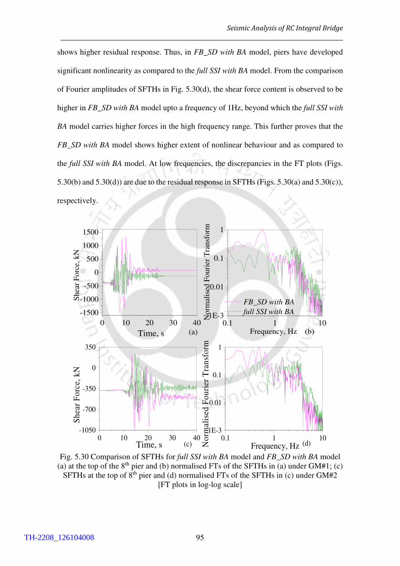
Seismic Analysis of RC Integral Bridge
______________________________________________________________________
95
shows higher residual response. Thus, in FB_SD with BA model, piers have developed
significant nonlinearity as compared to the full SSI with BA model. From the comparison
of Fourier amplitudes of SFTHs in Fig. 5.30(d), the shear force content is observed to be
higher in FB_SD with BA model upto a frequency of 1Hz, beyond which the full SSI with
BA model carries higher forces in the high frequency range. This further proves that the
FB_SD with BA model shows higher extent of nonlinear behaviour and as compared to
the full SSI with BA model. At low frequencies, the discrepancies in the FT plots (Figs.
5.30(b) and 5.30(d)) are due to the residual response in SFTHs (Figs. 5.30(a) and 5.30(c)),
respectively.
0 10 20 30 40
-1500
-1000
-500
0
500
1000
1500
FB_SD with BA full SSI with BA
(b)
Shear
Forc
e, k
N
Time, s (a)
0.1 1 101E-3
0.01
0.1
1
Frequency, Hz
Norm
alis
ed F
ouri
er T
ransf
orm
0 10 20 30 40-1050
-700
-350
0
350
(c) (d)
Sh
ear
Fo
rce,
kN
Time, s0.1 1 10
1E-3
0.01
0.1
1
Frequency, Hz No
rmal
ised
Fo
uri
er T
ran
sfo
rm
Fig. 5.30 Comparison of SFTHs for full SSI with BA model and FB_SD with BA model
(a) at the top of the 8th pier and (b) normalised FTs of the SFTHs in (a) under GM#1; (c)
SFTHs at the top of 8th pier and (d) normalised FTs of the SFTHs in (c) under GM#2
[FT plots in log-log scale]
TH-2208_126104008

5.7 Mean Maximum Response
______________________________________________________________________
96
5.7 Mean Maximum Response
Based on the analyses of the different models, the average of the maximum response is
evaluated from all the seven ground motions (Table. 5.2). For the linear and nonlinear
time history analyses, it is observed that for the B_FF, B_SSI and full SSI no BA models,
the mean peak response corresponding to the bending moment and shear force in piers
follow similar trends. Only B_FF model shows higher response as compared to the only
B_SSI and full SSI no BA models. In LTHA and NTHA, the mean peak lateral drifts at
deck level do not follow the trend as that observed for shear force and bending moment.
The observed mean peak drifts are higher in full SSI no BA model than the drift levels of
only B_FF and only B_SSI models. This occurs due to the underlying soil continuum
elements that tend to impart increase deformability of the bridge structure. Maximum
deck acceleration follows the usual trend but mean peak acceleration in nonlinear THA
is highest for nonlinear full SSI no BA model as nonlinearities in substructure and soil
influence the response of bridge superstructure in this case.
In linear THA, the residual response becomes the same as the static response from
staged gravity analysis. But to investigate the influence of nonlinearities in soil and
structure separately, two contemporary cases are considered, namely the (a) lin str+nl
soil no BA model and the (b) nl str+lin soil no BA model. The bending moment and shear
force response in piers of the lin str+nl soil no BA model are approximately 0.26 times
less and 1.67 times more than the response from the linear and nonlinear behaviours of
full SSI no BA model, respectively. On the other hand, the bending moment and shear
force response in piers of the nl str+lin soil no BA model are 0.19 times less and 1.18
times more than the response from the linear and nonlinear behaviours of the full SSI no
BA model, respectively. So, nonlinearity of structure is observed to govern the response
under the considered set of site specific ground motions for which the average PGA is
TH-2208_126104008

Seismic Analysis of RC Integral Bridge
______________________________________________________________________
97
0.48g. On the contrary, it is observed in Section 5.4.2, nonlinearity of soil tends to
dominate the response under low PGA of ground motions. Once the abutment backfill
soil is introduced in the full SSI no BA model, the bending moment and shear force get
further reduced by approximately 20% during its nonlinear behaviour. Residual shear
force is also the lowest for the nonlinear behaviour of the full SSI with BA model, but the
residual displacement in full SSI with BA model is more than nonlinear full SSI no BA
model. Deck acceleration and displacement are lower in lin str+nl soil no BA model as
compared to the nonlinear behaviours of full SSI no BA model and nl str+lin soil no BA
model. Because of soil nonlinearity, high frequency seismic waves get filtered and lesser
forces are imposed on the bridge structure. Residual displacement is lowest in nl str+lin
soil no BA model as compared to the values obtained in the nonlinear behaviour of all
other models. This is due to the occurrence of static drift as residual response at the end
of dynamic analysis.
Thus, after comparing the two contemporary cases, it is observed that the residual
response depends primarily on the deformation of the foundation soil. Under NTHA, the
shear force and bending moment response in piers for FB_SD no BA model are observed
to be higher than those obtained for full SSI no BA model. Residual shear force is higher
for the nonlinear behaviour of the full SSI no BA as compared to that in FB_SD no BA
model because of nonlinearity in the continuum soil domain. Similarly, response for
FB_SD with BA model is observed to be significantly higher than the nonlinear response
of full SSI with BA model with respect to the monitored bridge parameters, like bending
moment, shear force, moment-curvature and horizontal acceleration at deck level.
Overall, Table. 5.2 gives insight into the response of the structure under different input
motions (free field or SSI), material properties (linear or nonlinear) and boundary
conditions (presence or absence of abutment backfill soil).
TH-2208_126104008
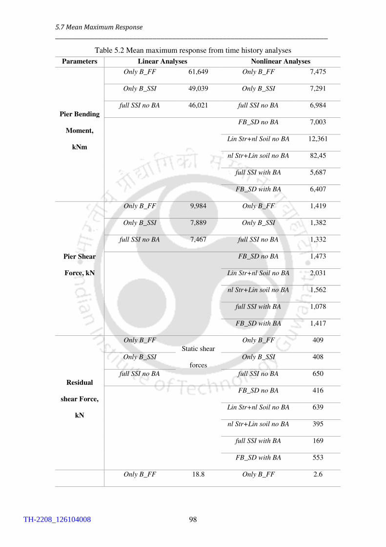
5.7 Mean Maximum Response
______________________________________________________________________
98
Table 5.2 Mean maximum response from time history analyses
Parameters Linear Analyses Nonlinear Analyses
Pier Bending
Moment,
kNm
Only B_FF 61,649 Only B_FF 7,475
Only B_SSI 49,039 Only B_SSI 7,291
full SSI no BA 46,021 full SSI no BA 6,984
FB_SD no BA 7,003
Lin Str+nl Soil no BA 12,361
nl Str+Lin soil no BA 82,45
full SSI with BA 5,687
FB_SD with BA 6,407
Pier Shear
Force, kN
Only B_FF 9,984 Only B_FF 1,419
Only B_SSI 7,889 Only B_SSI 1,382
full SSI no BA 7,467 full SSI no BA 1,332
FB_SD no BA 1,473
Lin Str+nl Soil no BA 2,031
nl Str+Lin soil no BA 1,562
full SSI with BA 1,078
FB_SD with BA 1,417
Residual
shear Force,
kN
Only B_FF Static shear
forces
Only B_FF 409
Only B_SSI Only B_SSI 408
full SSI no BA full SSI no BA 650
FB_SD no BA 416
Lin Str+nl Soil no BA 639
nl Str+Lin soil no BA 395
full SSI with BA 169
FB_SD with BA 553
Only B_FF 18.8 Only B_FF 2.6
TH-2208_126104008
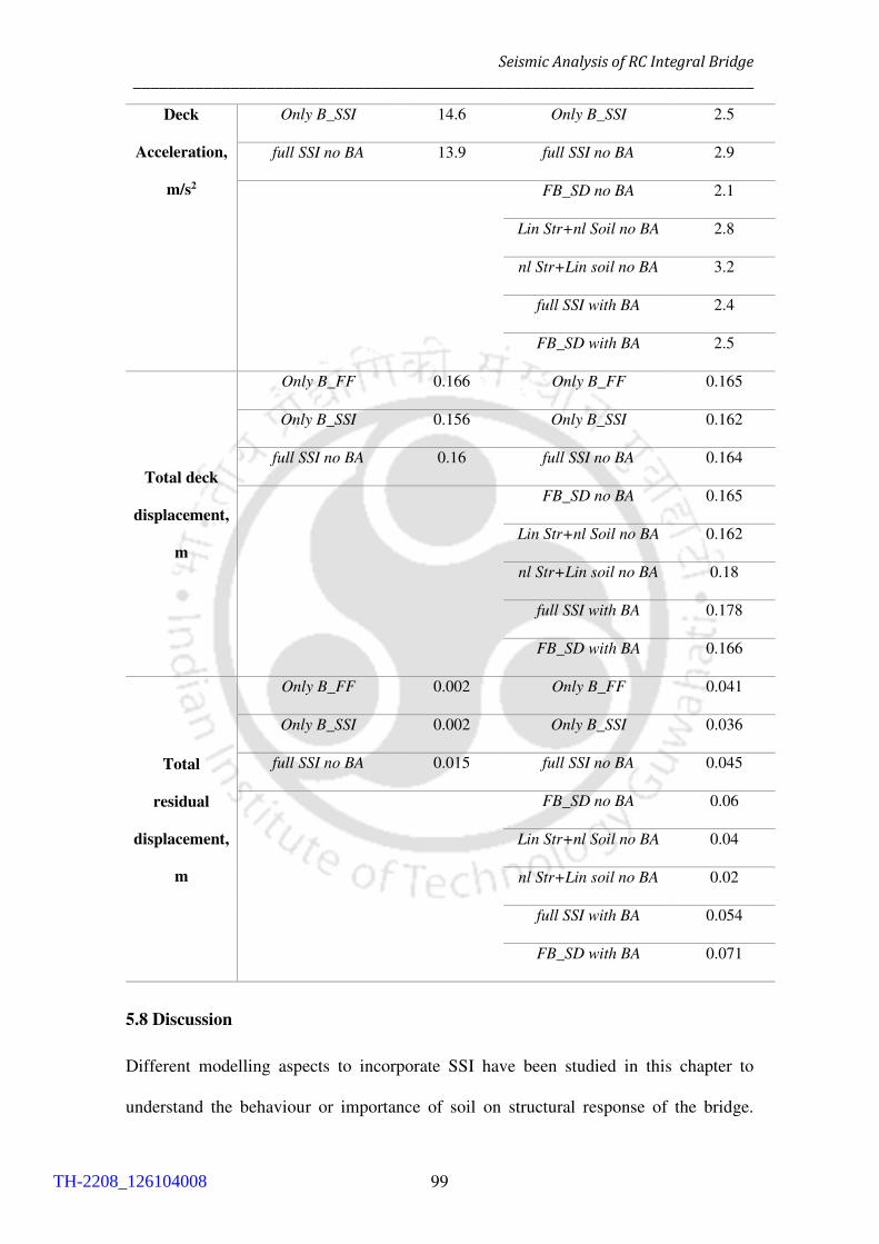
Seismic Analysis of RC Integral Bridge
______________________________________________________________________
99
Deck
Acceleration,
m/s2
Only B_SSI 14.6 Only B_SSI 2.5
full SSI no BA 13.9 full SSI no BA 2.9
FB_SD no BA 2.1
Lin Str+nl Soil no BA 2.8
nl Str+Lin soil no BA 3.2
full SSI with BA 2.4
FB_SD with BA 2.5
Total deck
displacement,
m
Only B_FF 0.166 Only B_FF 0.165
Only B_SSI 0.156 Only B_SSI 0.162
full SSI no BA 0.16 full SSI no BA 0.164
FB_SD no BA 0.165
Lin Str+nl Soil no BA 0.162
nl Str+Lin soil no BA 0.18
full SSI with BA 0.178
FB_SD with BA 0.166
Total
residual
displacement,
m
Only B_FF 0.002 Only B_FF 0.041
Only B_SSI 0.002 Only B_SSI 0.036
full SSI no BA 0.015 full SSI no BA 0.045
FB_SD no BA 0.06
Lin Str+nl Soil no BA 0.04
nl Str+Lin soil no BA 0.02
full SSI with BA 0.054
FB_SD with BA 0.071
5.8 Discussion
Different modelling aspects to incorporate SSI have been studied in this chapter to
understand the behaviour or importance of soil on structural response of the bridge.
TH-2208_126104008

5.8 Discussion
______________________________________________________________________
100
Although the effect of SSI is not considered in the structural design guidelines of the
integral bridge extensively, still the seismic behaviour of an integral bridge can
significantly differ for various types of input motion and material properties. Similarly,
difference in seismic response will be obtained by considering different modelling
approaches. The present study is intended to provide an overview of the variation in
response that can be obtained by adopting different modelling approaches. The easiest
way to consider SSI in modelling is to replace the soil continuum with suitable springs
and dashpots, representing the surrounding soil medium’s stiffness and damping
respectively. The influence of site-specific ground motions, as obtained from REXEL-
DISP software in the present study, on the seismic response of bridge-foundation-soil
system is also investigated. The ground motions have been selected in such a way that
the mean displacement spectrum from all the ground motions matches closely with the
site-specific target displacement spectrum. Limitations of analysis full SSI models are
they need computational as well as numerical efficiency, so to build the models high
performing computer systems are required which are also uneconomical. The execution
of analysis are time consuming due to the presence of soil domain. Limitations of analysis
FB_SD models are they are numerically efficient to model in different programs. But,
only spring-dashpots cannot depict the actual behaviour of realistic soil domain under
dynamic shaking. For say, past studies have been carried out to replicate actual soil
strength by assigning spring-dashpots at corresponding locations of soil domain. But, still
the response from these studies cannot matches the response of physical domain. Soil
liquefaction or excess pore water pressure dissipation cannot be incorporated through
spring-dashpots of soils.
The brief conclusions from the present study are stated below:
TH-2208_126104008

Seismic Analysis of RC Integral Bridge
______________________________________________________________________
101
1. For application of free field input (from site response analysis) at the fixed base of
bridge (only B_FF model), the structural response of substructure gets overestimated
for linear or nonlinear cases because the true behaviour of foundation embedded
inside continuous soil domain cannot be predicted from the response of a free-field
soil column at the desired depth.
2. When ground motion obtained from SSI effect is given as an input to the bottom of
the fixed base piers (only B_SSI model), the response is the quite similar as that
obtained from full SSI no BA model resulting in minimal kinematic interaction (i.e.
surficial, rigid foundations).
3. True incorporation of soil structure interaction results in reduced response as
compared to the uncoupled approach (as mentioned in 1). That observation is valid
for both linear (linear soil + linear structure) and nonlinear (linear soil + nonlinear
structure, nonlinear soil + nonlinear structure) behaviours of appropriate models.
4. Presence of backfill tends to reduce the force demand on the bridge structure, thus
reducing the nonlinear response considerably.
5. Under strong ground motions (PGA ≥0.48g for this study), the structural nonlinearity
governs the overall response of the bridge-foundation-soil system, whereas for low
intensity of shaking (PGA ≤0.1g for this study), soil nonlinearity tend to governs the
overall response. For the intermediate range of shaking, both influence the overall
behaviour.
6. The full SSI with BA model has the lowest response on bridge structure in NTHA. As
the backfill soil provides longitudinal restraints to the bridge, seismic force from
superstructure dissipates through backfill soil leading to reduced displacement level
in the bridge superstructure.
TH-2208_126104008

5.8 Discussion
______________________________________________________________________
102
7. Modelling of soil behaviour using Winkler spring-dashpot (API and BA) approach
tends to overestimate the seismic demand, thus, that approach can be possibly used
in case of seismic design of bridge-foundation-soil system.
8. As compared to the nonlinear behaviour of the full SSI no BA model and the full SSI
with BA model, the shear forces and bending moments in the piers are higher for
FB_SD no BA model and FB_SD with BA model because the foundation soil stiffness
is higher with the API force-displacement curves.
9. The response of the FB_SD no BA model is higher as compared to the full SSI no BA
model as API overestimates soil stiffness for foundation soil. Structural response is
amplified significantly at deck level for FB_SD no BA model and results in higher
forces and moments at pier-deck junctions.
10. For FB_SD with BA and full SSI with BA models, the former model is stiffer at super-
structural level and deforms in higher curvature after dynamic analysis, thus, the
observed nonlinearity is higher for this modelling approach and residual response
after dynamic analysis is also higher. Due to insufficient soil nonlinearity at
foundation and backfill region, FB_SD with/no BA models overestimate the overall
stiffness.
11. In full SSI with/no BA models, due to significant nonlinearity soil domain, bridge
response does not amplify at deck level; thus in this type of modelling bridge
response is lower as compared to the response obtained using simplistic SSI
modelling approach.
After the present study, it can be concluded that modelling of continuous soil domain to
assess SSI may not be always required in conventional seismic design, but from the
research point of view its gives detailed insight on the seismic behaviour of the bridge-
foundation-soil system. Spring-dashpot model can predict bridge response to some extent
TH-2208_126104008

Seismic Analysis of RC Integral Bridge
______________________________________________________________________
103
but as the intricacy in modelling increases, the response may start to deviate from the real
one. To study bridge design, modelling of abutment backfill is also a key parameter to
examine the response of the bridge. The spatial variability in the geometry of bridge
members has not been studied in this paper, but it is expected that it can surely show some
important design guidelines on SSI modelling approaches.
Nonlinear interface element has not been modelled in the present
study. In presence of interface elements in OpenSees models it is well known that the slip
and gap (debonding) due to soil-pile interaction and abutment backfill interaction can be
explicitly captured. Though, it is expected that it won’t be resulting in too much changes
in structural response because foundation soil is medium stiff clay and is nowhere near to
plastic failure under the site specific ground motions. Interface element can reflect the
nonlinear inelastic behaviour of soil which one could expect in reality.
TH-2208_126104008
______________________________________________________________________
Chapter 6
Study on Overall Length of Integral Bridge
6.1 Introduction
The influence of length of an integral bridge (IB) on the seismic behavior of the bridge in
investigated in this chapter. Though, parametric studies have been carried out in the past
on IBs (Erhan and Dicleli, 2017; Kong et al., 2016; Huang et al., 2008; Civjan et al.,
2007), but the influence of overall length has not been investigated on multispan IB with
RC pile foundation. In order to achieve the objective, finite element modelling of a 3D
IB, “inspired” by Humboldt Bay Middle Channel (HBMC) Bridge in California, USA, is
carried out using SAP2000 v.19.2.1 software (CSI, 2017). The FB_SD with BA model
overestimates the seismic response of bridge as compared to the full SSI with BA model
in Chapter 5 under dynamic loading. Thus, further analysis is carried out with spring-
dashpot model in 3D bridge to incorporate seismic SSI with one of the most accepted
structural analysis programs, SAP2000. Soil flexibility is modelled by two noded
nonlinear link elements. Four types of foundation soil are considered, namely (i) medium
stiff clayey soil, (b) soft clay, (c) loose sand and (d) dense sand, to incorporate nonlinear
dynamic Soil-Structure Interaction (SSI) at the soil-pile and abutment-backfill interfaces.
Among these four types of soil, nonlinear time history analysis is performed in medium
stiff clayey soil and loose sand. In loose foundation soil, the foundation becomes more
flexible and results in forming hinges at different depth of piles. In medium stiff clay, the
possibility of inelastic behaviour of the piers and the piles gets increased in an integral
bridge.
TH-2208_126104008
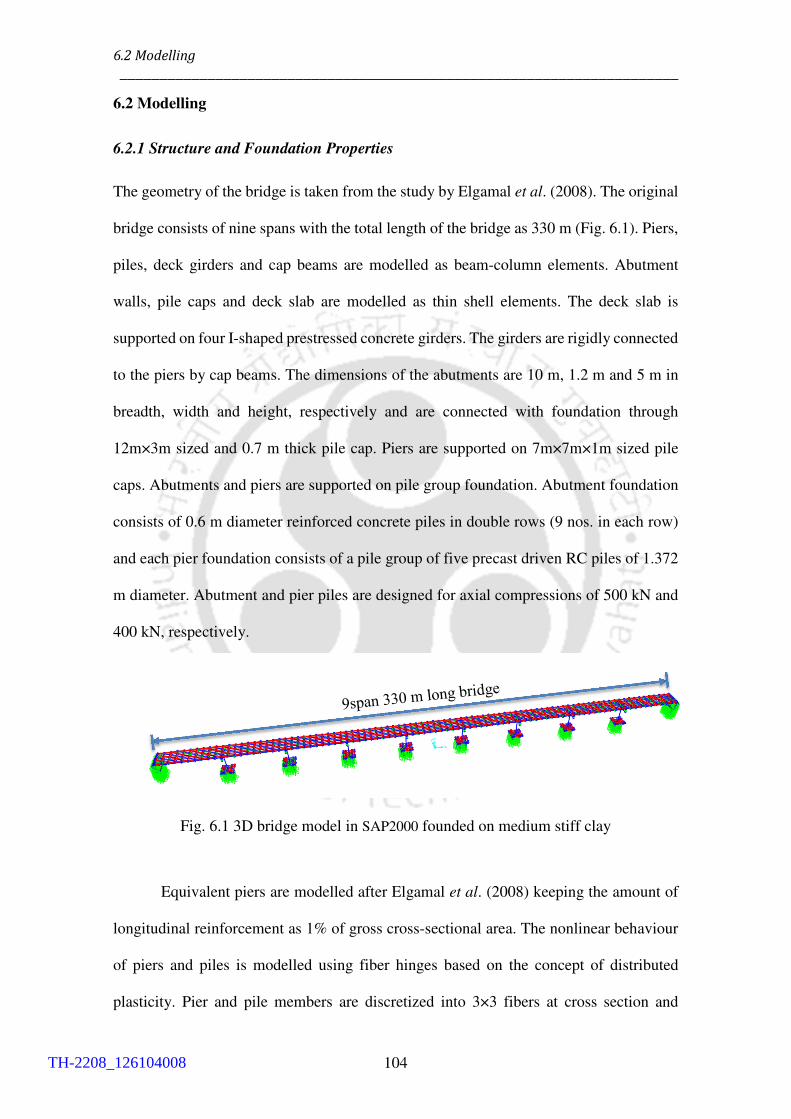
6.2 Modelling
______________________________________________________________________
104
6.2 Modelling
6.2.1 Structure and Foundation Properties
The geometry of the bridge is taken from the study by Elgamal et al. (2008). The original
bridge consists of nine spans with the total length of the bridge as 330 m (Fig. 6.1). Piers,
piles, deck girders and cap beams are modelled as beam-column elements. Abutment
walls, pile caps and deck slab are modelled as thin shell elements. The deck slab is
supported on four I-shaped prestressed concrete girders. The girders are rigidly connected
to the piers by cap beams. The dimensions of the abutments are 10 m, 1.2 m and 5 m in
breadth, width and height, respectively and are connected with foundation through
12m×3m sized and 0.7 m thick pile cap. Piers are supported on 7m×7m×1m sized pile
caps. Abutments and piers are supported on pile group foundation. Abutment foundation
consists of 0.6 m diameter reinforced concrete piles in double rows (9 nos. in each row)
and each pier foundation consists of a pile group of five precast driven RC piles of 1.372
m diameter. Abutment and pier piles are designed for axial compressions of 500 kN and
400 kN, respectively.
Fig. 6.1 3D bridge model in SAP2000 founded on medium stiff clay
Equivalent piers are modelled after Elgamal et al. (2008) keeping the amount of
longitudinal reinforcement as 1% of gross cross-sectional area. The nonlinear behaviour
of piers and piles is modelled using fiber hinges based on the concept of distributed
plasticity. Pier and pile members are discretized into 3×3 fibers at cross section and
TH-2208_126104008

Study on Overall Length of Integral Bridge
___________________________________________________________________
105
divided into 5 and 2 integration points along the length of the respective members. The
reinforcement details of the cross-sections, with HYSD 415 bars, are shown in Figs.
6.2(a), 6.2(b) and 6.2(c). Cover and core concrete material properties are considered from
Mander’s model (1984) with characteristics compressive strength of 30 MPa. The lengths
of the pier piles and abutment piles are changed in medium stiff clay and loose sand
depending on soil properties (Prakash and Sharma, 1990). In medium stiff clay and dense
sand, piles are 5.2 m in length and in loose sand, abutment and internal piles are 10 m and
15 m in length, respectively. In soft clay, abutment and intermediate piles are of 15 m and
10 m of length, respectively (Appendix D).
(a) (b) (c)
Fig. 6.2 Reinforcement detailing of cross-sections for (a) pier, (b) pier piles and (c)
abutment piles.
6.2.2 Properties of Soil links
The considered properties of all four types of soil are given in Table 6.1. Two noded link
elements are assigned at different depths of the pile foundation and abutment backwall
(Figs. 6.3(a) and 6.3(b)). The assigned link properties account for lateral bearing capacity
of soil at soil-pile interface (p-y), pile shaft skin friction (f-y) and pile tip load bearing
capacity (t-z). Nonlinear links are modelled using 2-noded multilinear plastic force-
deformation curves. To model the soil-pile interaction (SPI) for different types of soil, p-
y, f-y, t-z curves are calculated from API (2000) guidelines. For lateral Abutment-Backfill
TH-2208_126104008
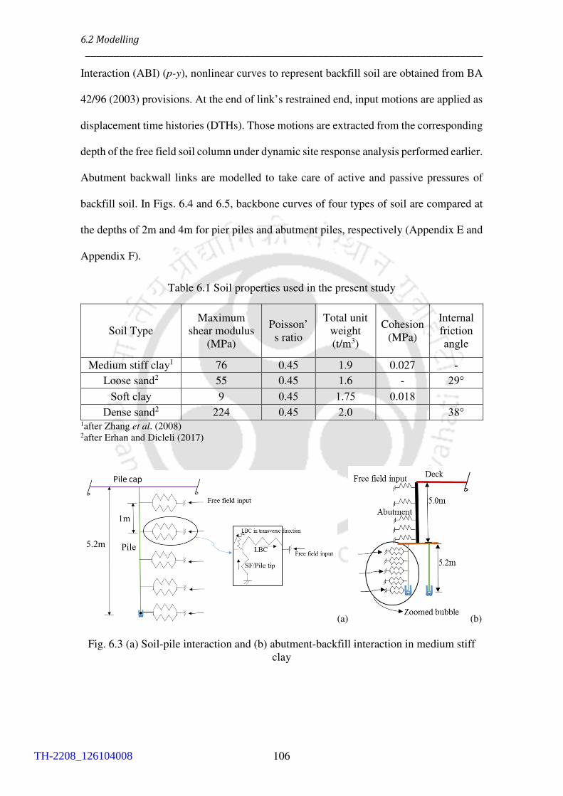
6.2 Modelling
______________________________________________________________________
106
Interaction (ABI) (p-y), nonlinear curves to represent backfill soil are obtained from BA
42/96 (2003) provisions. At the end of link’s restrained end, input motions are applied as
displacement time histories (DTHs). Those motions are extracted from the corresponding
depth of the free field soil column under dynamic site response analysis performed earlier.
Abutment backwall links are modelled to take care of active and passive pressures of
backfill soil. In Figs. 6.4 and 6.5, backbone curves of four types of soil are compared at
the depths of 2m and 4m for pier piles and abutment piles, respectively (Appendix E and
Appendix F).
Table 6.1 Soil properties used in the present study
1after Zhang et al. (2008) 2after Erhan and Dicleli (2017)
(a) (b)
Fig. 6.3 (a) Soil-pile interaction and (b) abutment-backfill interaction in medium stiff
clay
Soil Type
Maximum
shear modulus
(MPa)
Poisson’
s ratio
Total unit
weight
(t/m3)
Cohesion
(MPa)
Internal
friction
angle
Medium stiff clay1 76 0.45 1.9 0.027 -
Loose sand2 55 0.45 1.6 - 29°
Soft clay 9 0.45 1.75 0.018
Dense sand2 224 0.45 2.0 38°
TH-2208_126104008
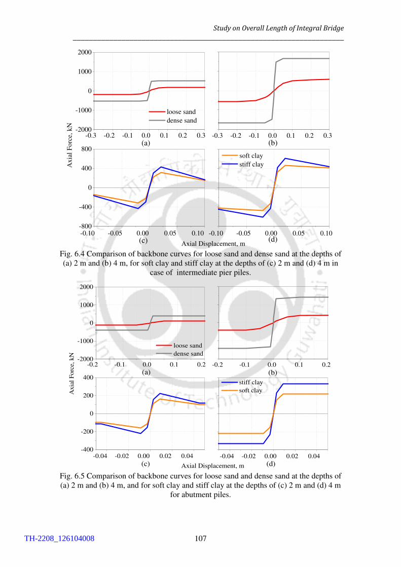
Study on Overall Length of Integral Bridge
___________________________________________________________________
107
-0.3 -0.2 -0.1 0.0 0.1 0.2 0.3-2000
-1000
0
1000
2000
loose sand
dense sand
Ax
ial
Fo
rce,
kN
-0.10 -0.05 0.00 0.05 0.10-800
-400
0
400
800 soft clay
stiff clay
Axial Displacement, m
-0.3 -0.2 -0.1 0.0 0.1 0.2 0.3
(a)
-0.10 -0.05 0.00 0.05 0.10(c) (d)
(b)
Fig. 6.4 Comparison of backbone curves for loose sand and dense sand at the depths of
(a) 2 m and (b) 4 m, for soft clay and stiff clay at the depths of (c) 2 m and (d) 4 m in
case of intermediate pier piles.
-0.2 -0.1 0.0 0.1 0.2-2000
-1000
0
1000
2000
loose sand
dense sand
Axia
l F
orc
e, k
N
-0.04 -0.02 0.00 0.02 0.04-400
-200
0
200
400 stiff clay
soft clay
Axial Displacement, m
-0.2 -0.1 0.0 0.1 0.2
-0.04 -0.02 0.00 0.02 0.04
(c) (d)
(b)(a)
Fig. 6.5 Comparison of backbone curves for loose sand and dense sand at the depths of
(a) 2 m and (b) 4 m, and for soft clay and stiff clay at the depths of (c) 2 m and (d) 4 m
for abutment piles.
TH-2208_126104008

______________________________________________________________________
108
6.3 Analysis
In the first part of the analysis, to investigate the effect of length, the two end spans of the
9 span 330 m long integral bridge (IB) are removed so that the bridge becomes a 7 span
bridge of 257 m. Further successive removals of two end spans, the bridge transform into
a 5 span bridge of 184 m length and a 3span bridge of 112 m length (in Fig. 6.6). End
spans of the bridge are removed to reduce the overall length of bridge. From the seven
real record scaled ground motions, the GM#1 is replaced by Irpinia earthquake at ALT
station on 23 Nov. 1980 having scaled PGA of 3.46 m/s2. GM#2 is retain the same which
has been chosen for previous study in Chapter 5. The chosen ground motions
displacement spectra are specified in Fig. 6.7(a). Figs. 6.7(b) and 6.7(c) represent the
Acceleration Time Histories (ATH) of the chosen GMs. In Figs. 6.7(d) and 6.7(e), Fourier
transforms of GM#1 and GM#2 are plotted and natural frequencies of different bridge
models considered are marked for both the foundation soil type. The natural frequencies
of different bridge models are spreaded over below 1Hz of frequency. Seismic energy is
higher beyond 1Hz of frequency for GM#1 and distributed over large frequency range for
GM#2. Under different GMs, input DTHs at the end of fixed pile links are different. In
Table 6.2, the natural periods of the bridges with different spans are shown for the four
types of foundation soil. The bridge becomes stiffer with decreasing number of spans. To
study the effect of length on seismic behaviour of bridge, nonlinear time history analysis
(NTHA) is carried out in medium stiff clay and loose sand foundation soil under GM#1
and GM#2. In the 2nd part of the study, the damaged 9span bridge is retrofitted by
encasement method in all four types of foundation soils and the comparison of response
under GM#1 only is discussed in the next chapter.
TH-2208_126104008
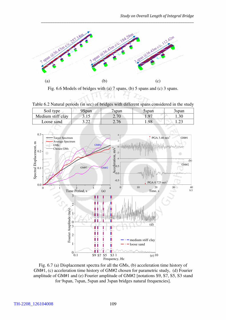
Study on Overall Length of Integral Bridge
___________________________________________________________________
109
(a) (b) (c)
Fig. 6.6 Models of bridges with (a) 7 spans, (b) 5 spans and (c) 3 spans.
Table 6.2 Natural periods (in sec) of bridges with different spans considered in the study
Soil type 9Span 7span 5span 3span
Medium stiff clay 3.15 2.70 1.97 1.30
Loose sand 3.22 2.76 1.98 1.23
-4
-2
0
2
4
Acc
eler
atio
n,
m/s
2
PGA 3.46 m/s2
0 10 20 30 40
-0.5
0.0
0.5
(b)
Time, s
PGA 0.725 m/s2
(c)
GM#1
GM#2
0.1 1 100
1
2
3
0
1
2
3
(d)
medium stiff clay
loose sand
Frequency, Hz
Fouri
er A
mpli
tude
(m/s
)
S9 S7 S5 S3 (e)
Fig. 6.7 (a) Displacement spectra for all the GMs, (b) acceleration time history of
GM#1, (c) acceleration time history of GM#2 chosen for parametric study, (d) Fourier
amplitude of GM#1 and (e) Fourier amplitude of GM#2 [notations S9, S7, S5, S3 stand
for 9span, 7span, 5span and 3span bridges natural frequencies].
0 1 2 3 40.0
0.1
0.2
0.3
GM#3
GM#1
Sp
ectr
al D
isp
lace
men
t, m
Time Period, s
Target Spectrum
Average Spectrum
GMs
Chosen GMs
(a)
GM#2
TH-2208_126104008
6.4 Results
______________________________________________________________________
110
6.4 Results
6.4.1 Response for medium stiff clay soil
In medium stiff clay foundation soil, inelastic response is observed at the top of 3rd (Fig.
6.8(a)) and 6th piers and at their respective pile groups for 9span bridge under GM#1.
Under GM#1, due to higher intensity of PGA (= 3.46 m/s2), shear force has significant
variation among 9span, 7span and 5span bridges after PGD at t = 12.06 s. The increase
of nonlinearity leads to maximum residual shear force (SF) for the 9span and 7span
bridges. From Figs. 6.8(a) and 6.8(c), 5span bridge pier is showing linear behavior which
also results in insignificant residual SF in NTHA under GM#1. Response of 5span and
3span bridges are similar from the aspect of structural members. Thus it shows, as in the
case of jointless bridge, forces coming from foundation to structure increase with
increasing length of the bridge. Under GM#2, linear elastic behavior is observed in piers
for all the bridges (Fig. 6.8(b)). Thus, only the results of 9span bridge are shown for the
pier response in the following study under GM#2. In Fig. 6.8(c), the moment-rotation
response at 1.25 m from the top of 3rd pier are shown. Inelastic behavior of the piers is
observed in the 9span and 7span bridges after the dynamic analyses. For the 5span bridge,
very narrow loops, signifying low level of inelasticity, are formed under GM#1. Under
GM#2, i.e., at low intensity of PGA (i.e. 0.725 m/s2), SFTH at the top of 3rd pier in 9span
bridge shows insignificant residual response (Fig. 6.8(b)) and linear moment-rotation
response is obtained at the end of dynamic analysis (Fig. 6.8(d)).
TH-2208_126104008

Study on Overall Length of Integral Bridge
___________________________________________________________________
111
0 10 20 30-1050
-700
-350
0
350
9 span
7 span
5 span
(a) (b)
Sh
ear
Fo
rce,
kN
Time, s
(c) (d)
0 10 20 30
-0.6 -0.4 -0.2 0.0 0.2
-9000
-6000
-3000
0
3000
Rotation (x 0.01rad)
Mo
men
t, k
Nm
-0.6 -0.4 -0.2 0.0 0.2
Fig. 6.8 Shear force response at the top of 3rd pier under (a) GM#1 and (b) GM#2;
moment-rotation response at the top of 3rd pier under (c) GM#1 and (d) GM#2 in
medium stiff clay soil.
Displacement time histories (DTHs) at the top and bottom of the abutments are
monitored under GM#1 in Figs. 6.9(a) and 6.9(b), respectively. At the top of the
abutment, the residual displacements of the 9span, 7span and 5span bridges are observed
as 0.166 m, 0.123 m and 0.044 m, respectively. Those also signify that the 9span bridge
has undergone the highest extent of nonlinearity. Significant deformation is accumulated
at the integral deck-abutment-backfill joint. Similar response is observed at the bottom of
abutment as shown in Fig. 6.9(b). Under GM#2 for 9span bridge in Fig. 6.9(c), the top
and bottom DTHs of abutment are quite similar and the bridge model has no significant
residual response after dynamic analysis; this also confirms linear elastic behavior of the
bridge.
At the depth of 1.25 m of abutment piles, moment rotation curves are shown in
Figs. 6.10(a) and 6.10(b) under GM#1 and GM#2, respectively. Under GM#1and GM#2,
abutment piles are showing linear elastic response for all considered bridge spans. In
contrary to that, extensive nonlinearity of pier piles at the depth range of 1–2 m are
TH-2208_126104008

6.4 Results
______________________________________________________________________
112
observed in Figs. 6.10(c) under GM#1. Under GM#1, the piles of the 3rd pier foundation
in 9span, 7span and 5span bridge models undergo severe nonlinearity, along with inelastic
behavior of the pier piles in 3span bridge too. Under GM#2, pier piles exhibit insignificant
nonlinear response for all the bridges in medium stiff clay foundation soil.
0 10 20 30
0.0
0.2
GM#2GM#1
(c)(b) Time, s
9 span
7 span
5 span
Dis
pla
cem
ent,
m
(a)
GM#1
0 10 20 30 0 10 20 30
Abutment top
Autment bottom
Fig. 6.9 Displacement time histories (DTHs) for bridges of 9span, 7span and 5span at
(a) top of abutment and (b) bottom of abutment under GM#1, (c) DTHs of 9span bridge
under GM#2 in medium stiff clay foundation soil.
-400
-200
0
200
400
(a) (b)
(c) (d)-1.0 -0.5 0.0 0.5 1.0
-400
-200
0
200
400
9span
7span
5span
3span
Rotation (x0.01rad)
Mo
ment,
kN
m
-1.0 -0.5 0.0 0.5 1.0
Fig. 6.10 Moment-rotation response of abutment pile under (a) GM#1 and (b) GM#2,
and for pier pile under (c) GM#1 and (d) GM#2 in medium stiff clay foundation soil at
the depth of 1.25 m from ground level.
TH-2208_126104008

Study on Overall Length of Integral Bridge
___________________________________________________________________
113
6.4.2 Response for loose sand
Under GM#1, the 9span bridge shows more residual displacement at the top of left
abutment as compared to the 7span bridge (Fig. 6.11(a)). However, the residual
displacement at the bottom of the abutment for the 7span bridge is almost the same as
9span bridge because the deformation decreases from deck to foundation level (Fig.
6.11(b)). The overall deck displacement of a bridge model in loose sand is less as
compared to the deck displacement of the same model in medium stiff clayey soil. 7span
bridge superstructure also results in insignificant residual deformation and remains linear
elastic after DTHA. DTHs at the top and the bottom locations of left abutment are plotted
in Fig. 6.11(c) for 9span bridge under GM#2 which shows similar response in DTHA.
0 10 20 30
0.0
0.2
0.4
GM#2
GM#1
(c)(b) Time, s
9 span
7 span
Dis
pla
cem
ent,
m
(a)
GM#1
0 10 20 30 0 10 20 30
Abutment top
Abutment bottom
Fig. 6.11 Displacement time histories (DTHs) for 9span and 7span bridges at (a) top of
abutment and (b) bottom of abutment under GM#1, (c) DTHs for 9span bridge under
GM#2 in loose sand.
Unlike the previous case, pile foundation in loose sand helps the foundation to
respond in a more flexible manner. Under GM#1, it is observed that the residual SF at the
top of 3rd pier of the 9span bridge is insignificant like that for the 7span bridge (Fig.
6.12(a)). However, the obtained moment-rotation response at 1.2 m from the top of the
3rd pier shows marginally nonlinear response and linear elastic response for 9span and
7span bridges (Fig. 6.12(c)), respectively. Thus, the bridge substructure behaves in a
linear elastic manner in loose foundation soil under GM#1 for the 7span, 5span and 3span
bridges. Where, under GM#2, at the top of 3rd pier, SFTH is shown in Fig. 6.12 (b) and
TH-2208_126104008

6.4 Results
______________________________________________________________________
114
the pier is linear elastic from moment rotation response at the location of 1.2 m from the
top of the pier (Fig. 6.12 (d)).
0 10 20 30
-1200
-800
-400
0
400
9 span
7 span
(a) (b)
Sh
ear
Fo
rce,
kN
Time, s
(c) (d)
0 10 20 30
-0.6 -0.4 -0.2 0.0 0.2
-8000
-4000
0
4000
Rotation (x 0.01rad)
Mo
men
t, k
Nm
-0.6 -0.4 -0.2 0.0 0.2
Fig. 6.12 Under GM#1 (a) shear force time history, (b) moment rotation response, under
GM#2 (c) shear force time history, (b) moment rotation response at the top of 3rd pier,
in loose sand
Although the bridge substructure does not show significant nonlinearity for the
9span bridge, the abutment piles and the pier piles show inelastic behavior under GM#1
(Figs. 6.13(a) and 6.13(c)). The moment-rotation response of the pile section at the depth
of 1.25 m below ground level shows more nonlinearity for the pier piles in 9span bridge.
However, for bridges with lesser spans, nonlinearity has reduced in foundation level. In
Figs. 6.13(b) and 6.13(d), the moment-rotation curves of the abutment pile and pier pile
are shown under GM#2, respectively and for all the locations of foundation part, piles
have formed narrow inelastic loops. So, unlike in medium stiff clayey foundation soil,
only the 9span bridge shows nonlinear response of piers in loose sand under GM#1.
Though, the rest of the considered span of bridge models have nonlinear response limited
to the foundation part only. Plastic hinge formation is limited to a depth of 8 m along the
TH-2208_126104008

Study on Overall Length of Integral Bridge
___________________________________________________________________
115
pile, so special attention is needed to design the pile foundation in soft soil for larger
jointless bridges.
-150
-75
0
75
150
(a) (b)
(c) (d)-0.4 -0.2 0.0 0.2 0.4
-150
-75
0
75
150
Mom
ent,
kN
m
9span
7span
5span
Rotation (x 0.01rad)
-0.4 -0.2 0.0 0.2 0.4
Fig. 6.13 Moment-rotation response of abutment piles under (a) GM#1 and (b) GM#2,
and of pier piles under (c) GM#1 and (d) GM#2 in loose sand at the depth of 1.25 m
from ground level.
6.4.3 Comparison of response in loose sand and medium clay soil
In Fig. 6.14, at the depth of 2 m and 4 m, the p-y response of the soil link elements is
monitored for left abutment piles in both types of foundation soil. In case of medium stiff
clay and loose sand, the soil links show linear elastic behaviour. Soil links in stiff clay
are deforming less than 0.001 m at both the monitored depths of 2 m and 4 m of abutment
pile. Thus, it can be concluded that in stiff clayey soil, soil links undergo less relative
deformations and impose higher seismic forces on the piles; this leads to formation of
plastic hinges at different locations in the piles.
TH-2208_126104008
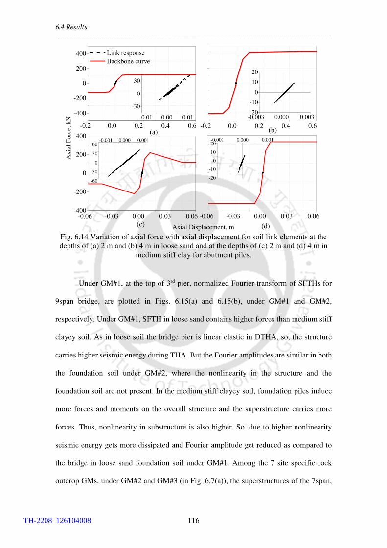
6.4 Results
______________________________________________________________________
116
-0.2 0.0 0.2 0.4 0.6
-400
-200
0
200
400
Ax
ial
Fo
rce,
kN
-0.06 -0.03 0.00 0.03 0.06-400
-200
0
200
400
Axial Displacement, m
-0.2 0.0 0.2 0.4 0.6
-0.06 -0.03 0.00 0.03 0.06
Link response
Backbone curve
-0.01 0.00 0.01
-30
0
30
(c) (d)
(b)(a)
-0.003 0.000 0.003-20
-10
0
10
20
-20
-10
0
10
20-0.001 0.000 0.001
-60
-30
0
30
60-0.001 0.000 0.001
Fig. 6.14 Variation of axial force with axial displacement for soil link elements at the
depths of (a) 2 m and (b) 4 m in loose sand and at the depths of (c) 2 m and (d) 4 m in
medium stiff clay for abutment piles.
Under GM#1, at the top of 3rd pier, normalized Fourier transform of SFTHs for
9span bridge, are plotted in Figs. 6.15(a) and 6.15(b), under GM#1 and GM#2,
respectively. Under GM#1, SFTH in loose sand contains higher forces than medium stiff
clayey soil. As in loose soil the bridge pier is linear elastic in DTHA, so, the structure
carries higher seismic energy during THA. But the Fourier amplitudes are similar in both
the foundation soil under GM#2, where the nonlinearity in the structure and the
foundation soil are not present. In the medium stiff clayey soil, foundation piles induce
more forces and moments on the overall structure and the superstructure carries more
forces. Thus, nonlinearity in substructure is also higher. So, due to higher nonlinearity
seismic energy gets more dissipated and Fourier amplitude get reduced as compared to
the bridge in loose sand foundation soil under GM#1. Among the 7 site specific rock
outcrop GMs, under GM#2 and GM#3 (in Fig. 6.7(a)), the superstructures of the 7span,
TH-2208_126104008

Study on Overall Length of Integral Bridge
___________________________________________________________________
117
5span and 3span bridges remain linear elastic, with observation of marginal inelasticity
for piles in both the types of soil. Under GM#1 and rest of them, 9span bridge has failed
either at different locations of piles or at both piles and piers, which is followed by the
failure of piles in 7span, 5span and 3span bridges. In Fig. 6.15(c), comparison of average
Fourier amplitude of seven rock outcrop GMs and output average Fourier transform of
ATHs monitored at the top of 3rd pier in SAP2000 are plotted. Output Fourier amplitude
is considerably higher throughout 0.1–10 Hz frequency range. This is because of the
presence of structural and soil nonlinearities as seismic waves get amplified during
vertical propagation from bedrock to superstructure level. In Table 6.3, overall behaviour
of bridge piles and piers are summed up for all the considered bridge spans in DTHA.
0.1 1 100.0
0.2
0.4
0.6
0.8
1.0
(b) Frequency, HzN
orm
aliz
ed F
ou
rier
Tra
nsf
orm
(a)0.1 1 10
medium stiff clay
loose sand
0.1 1 101E-3
0.01
0.1
1
10
Fouri
er A
mpli
tude,
m/s
Frequency, Hz
output median
input average target
output mean
(c)
Fig. 6.15 (a) Normalized Fourier transform of SFTH under GM#1, (b) normalized
Fourier transform of SFTH under GM#2 at the top of 3rd pier for 9span bridge and (c)
comparison of Fourier amplitude at input and output stages of analysis for 9span bridge
in medium stiff clayey soil.
TH-2208_126104008

6.4 Results
______________________________________________________________________
118
Table 6.3 Behavior of bridge members after DTHA in medium stiff clay and loose sand
Members GM Soil type 9span 7span 5span 3span
Piers
GM#1
Medium stiff clay inelastic inelastic elastic elastic
Loose sand inelastic elastic elastic elastic
GM#2
Medium stiff clay elastic elastic elastic elastic
Loose sand elastic elastic elastic elastic
Pier piles
GM#1
Medium stiff clay inelastic inelastic inelastic inelastic
Loose sand inelastic inelastic inelastic inelastic
GM#2
Medium stiff clay inelastic inelastic inelastic elastic
Loose sand inelastic inelastic inelastic elastic
Abutment
piles
GM#1
Medium stiff clay elastic elastic elastic elastic
Loose sand inelastic inelastic inelastic inelastic
GM#2
Medium stiff clay elastic elastic elastic elastic
Loose sand inelastic inelastic inelastic elastic
6.4.4 Response of bridge in dense sand and soft clay
Response of the bridge in dense sand and soft clay foundation can be studied from
backbone curves (Figs. 6.4 and 6.5) of respective soils. In dense sand, backbone curves
are steeper, which means links will be carrying higher forces as compared to the loose
sand and higher response would be imposed on the bridge foundation. Thus, extensive
nonlinearity is expected to govern the response of the bridge substructure. So, even
bridges with lesser number of spans can be expected to show nonlinear response in dense
sand. In soft clay, backbone curves of the links are less steep than those for stiff clay.
Thus, the imposed forces on the piles will reduce. So, response of substructure will also
reduce and nonlinearity is expected to be lesser than in medium stiff clayey soil.
TH-2208_126104008

Study on Overall Length of Integral Bridge
___________________________________________________________________
119
6.5 Summary
To provide a closure to this study, dynamic analysis is carried out with all seven scaled
GMs from REXEL-DISP. Only under GM#2 and GM#3, the piers are linear elastic in
DTHA. From the present study, it can be concluded that the bridge with maximum
number of spans attracts more forces and moments than the shorter ones as there is no
intermediate joint or bearing to dissipate seismic energy at superstructure level. Pile
foundation in loose foundation soil can become very flexible and deform easily, thus
nonlinearity gets reduced in the foundation members. Hence, failure of structural
members can be limited to the foundation part only. On the other hand, it can also result
in seismically vulnerable foundation which will not be suitable for performance in severe
seismic zone. For this specific bridge model, the 3rd and the 6th piers and the
corresponding pile groups are more susceptible to dynamic shaking. Large span bridges
(with overall length more than 300 m) in medium stiff clayey soil are likely to sustain
higher seismic damage during strong earthquake shaking due to imposition of more forces
from soil to piles. It is observed that the 9span and 7span bridges undergoes extensive
inelastic behavior as compared to the 5span and 3span bridges after DTHA under GM#1
in medium stiff clayey soil. Major nonlinearity is seen at pier pile sections for all bridge
spans in medium stiff clayey soil. Hence, it won’t be advisable to construct 9span and
7span bridge in these specific geological conditions. In loose sand, 9 span bridge shows
insignificant nonlinearity in piers and foundation piles whereas, substructure is
completely linear elastic for 7span, 5span and 3span bridges in loose sand under GM#1.
Thus, if proper measures are taken in further pile and pier designing, 9span bridge in
loose sand and upto 5span bridge in medium stiff clay soil can be constructed.
Site response analysis must be carried out prior to design of integral abutment
bridge in stiff clayey soil. Specially, the influence of SSI on seismic behaviour of
TH-2208_126104008

6.5 Summary
______________________________________________________________________
120
foundation tends to be significant during earthquake shaking. Moreover, piles in stiffer
soil attract more seismic forces under earthquake motion which results in increased
nonlinear behaviour of the foundation. Seismic design of piles also becomes a critical
aspect due to their role in the soil-pile-bridge interaction during transfer of seismic forces.
Apart from the pile group, proper backfill soil is required to withstand transfer of dynamic
forces generated during shaking of bridge. Backfill soil should not be too stiff to impose
extra load on bridge neither too loose to permit large lateral deformations of the bridge.
Thus, detailed guidelines are required for proper seismic design of the piers and
foundation piles in order to obtain desirable seismic behaviour of the integrated soil-pile-
bridge system.
Depending on proper geological investigation and site specific characteristics, the
integral bridges should be constructed so that due to larger length, yielding of foundation
piles can be prevented. In that case, foundation needs to be designed more carefully with
higher endurance capacity and proper retrofitting of foundation should be a scope to make
the bridge more sustainable under high intensity GMs.
TH-2208_126104008

______________________________________________________________________
Chapter 7
Retrofitting of Pile Foundation
7.1 Introduction
In the previous chapter, nonlinear behaviors of the abutment piles and the pier piles are
observed along with large displacement at deck level for the bridge with the longest span
under GM#1. As the mentioned response can lead to seismic failure of the overall bridge
structure, one of the possible retrofitting measures for the pile foundation is discussed in
this chapter. In this retrofitting method, RC piles are added along the periphery of the
abutment pile cap and the pier pile cap, and jet grouting is carried out in the surrounding
region of each new pile. In the first stage of analysis, the new piles encased in jet grouting
are considered only below the abutments and the response are compared with the response
of the original bridge model without the new piles. Then, new piles encased in jet grouting
are added below two piers of the bridge. So, in the second stage of analysis, the response
of the bridge model with retrofitted abutment and pier pile foundations is compared with
the response of the bridge model with only retrofitted abutment pile foundation. For both
the stages, the nonlinear response of individual pile gets reduced below the abutments
and the piers. This further leads to the reduction of nonlinearity in piers as well as
deformation at the deck level and reflects the effectiveness of the retrofitting method.
Although the response of the retrofitted bridge will change with the height of the
abutment, the scope of the present study is limited to the investigation of the bridge
response for the two stages of retrofitting mentioned earlier. To the best of the author’s
knowledge, numerical study of the mentioned retrofitting method has not been carried
out previously. Detailed parametric studies involving multiple ground motions and other
bridge parameters can be carried out separately in future.
TH-2208_126104008

7.2 Retrofitting of RC Pile Foundation _____________________________________________________________________
122
7.2 Retrofitting of RC Pile Foundation
In the past, different methods of retrofitting of RC pile foundation have been attempted
and some of those studies have been discussed in Chapter 2. The selection of any
particular method depends on the cost as well as the difficulty level in the installation
procedure. Among the different methods, extension of existing pile cap and addition of
new piles in the foundation is very difficult and cost ineffective. Similarly, thickening of
pile cap involves challenges in construction and also required significant vertical
clearance. Although micropiles can be added surrounding the pile cap, proper seismic
strengthening of the overall pile group may not be achieved in absence of grouting of the
micropiles. If grouting is implemented in an existing pile foundation, the increase in the
lateral bearing capacity of the pile group is expected to be less than the increase in the
lateral bearing capacity achieved through jet grouting around installed new piles. So, the
present study focuses on the numerical modeling of additional RC piles surrounding the
pile cap and embedded in jet grouting which can enhance lateral bearing capacity and
bear the additional passive pressure generated during earthquake shaking. The properties
of the jet grouting used in the present studies (He et al., 2016) are: injection pressure of
grout = 27MPa; water cement ratio of grout = 1:1; life rate = 0.025 m/min; rotation speed
= 18 rad/min; replacement ratio of cement = 33%; modulus of elasticity = 120 MPa;
tensile strength = 0.18 MPa.
7.2.1 Modelling of encasement method
In the first stage of the present study, encasement method is incorporated by encasing RC
piles in jet grouting around the periphery of the pile cap below each abutment. From the
NTHA of the 9-span integral bridge model under GM#1, it is observed that the bending
moment diagram in the abutment piles shows significant moment upto a depth of 4 m
from the ground level for soft clay (Fig. 7.1(a) and loose sand (Fig. (7.1(b)), respectively.
TH-2208_126104008

Retrofitting of Pile Foundation
______________________________________________________________________
123
Below the depth of 4m from soil surface, mostly linear elastic behavior of piles is
observed. So, the length of the new encased piles is considered as 4 m for the abutment
pile foundation. The new encased piles are modelled with a minimal diameter of 0.4 m
considered as cast in place driven RC piles. Henceforth, the original bridge model before
retrofitting (in Fig. 6.1) and the retrofitted bridge model only at abutment foundation, will
be referred to as M1 and M2 models, respectively.
(a) (b)
Fig. 7.1 Maximum bending moment diagram (not to scale) in piles below left abutment
for the original bridge model in (a) soft clay at t =12.52 s and (b) loose sand at t = 12.56
s under GM#1.
The schematic diagrams of the retrofitted abutment foundation for M2 model are
shown in Figs. 7.2(a) to 7.2(c). In the numerical model of the encased new piles, the
spring-dashpot elements representing the lateral strength, lateral stiffness and the
damping characteristics of the grout are modelled in series configuration with the soil
spring-dashpot elements. The force-displacement characteristic corresponding to the
lateral bearing capacity of jet grouting, is taken from He et al. (2016). For the original
piles, the same spring-dashpot elements used in the study in Chapter 6, are modelled.
(a)
TH-2208_126104008

7.2 Retrofitting of RC Pile Foundation _____________________________________________________________________
124
(b) (c)
Fig. 7.2 (a) Schematic diagram of retrofitted abutment foundation in plan,(b) vertical
section A-A (h1 = height of abutment pile; h2 = height of encasement pile) and (c)
spring-dashpot model of the abutment and its retrofitted foundation in medium stiff
clay.
7.2.2 Encasement method at pier pile foundation
For M2 model, the maximum bending moments are observed in the piles below the 3rd
and the 6th piers (Fig. 7.3). Like the extent of the significant bending moment diagram
observed in the original abutment piles, the pier piles are also subjected to significant
bending moment till a depth of 4 m during NTHA under GM#1. So, the length of new
encased piles is kept as 4 m. However, the diameter of the new encased piles is considered
as 0.8 m. To integrate the new encased piles with the original pile cap, the original pile
cap is extended (Wang, 2015) equally along both the directions from the size of 7m×7m
to 8m×8m in plan. The schematic diagram of the retrofitted pier pile foundation is shown
in Fig. 7.4. Henceforth, the bridge model with retrofitted abutment and pier pile
foundations will be referred to as M3 model.
TH-2208_126104008
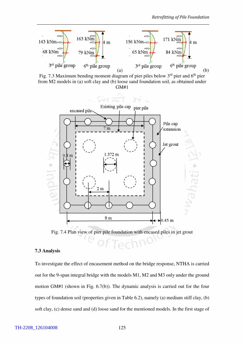
Retrofitting of Pile Foundation
______________________________________________________________________
125
(a) (b)
Fig. 7.3 Maximum bending moment diagram of pier piles below 3rd pier and 6th pier
from M2 models in (a) soft clay and (b) loose sand foundation soil, as obtained under
GM#1
Fig. 7.4 Plan view of pier pile foundation with encased piles in jet grout
7.3 Analysis
To investigate the effect of encasement method on the bridge response, NTHA is carried
out for the 9-span integral bridge with the models M1, M2 and M3 only under the ground
motion GM#1 (shown in Fig. 6.7(b)). The dynamic analysis is carried out for the four
types of foundation soil (properties given in Table 6.2), namely (a) medium stiff clay, (b)
soft clay, (c) dense sand and (d) loose sand for the mentioned models. In the first stage of
TH-2208_126104008

7.4 Results _____________________________________________________________________
126
analysis, the dynamic response of M1 and M2 models are compared and in the second
stage of the analysis, the response of M2 and M3 models are compared. In Table 7.1, the
natural periods of the M1 and M2 models in four different types of foundation soil for are
compared. The comparison reflects the higher stiffness of M2 model as compared to the
M1 model for all the types of soil.
Table 7.1 Natural period of 9 span integral bridge model in different foundation soils
Model Medium stiff clay Loose sand Soft clay Dense sand
M2 2.49 2.60 2.65 2.38
M1 3.15 3.22 3.25 3.15
7.4 Results
7.4.1 Comparison between M1 and M2 models
In Fig. 7.5, the moment-rotation response of the original abutment piles and the pier piles
at a depth of 1.25 m from soil surface are compared for M1 and M2 models. Although
the moment-rotation response gets reduced for M2 model in all the types of soils except
dense sand for abutment piles (Figs. 7.5(a) and 7.5(c)). For M1 and M2 models, in
medium stiff clay and dense sand, pier piles are going through extensive nonlinearity
(Figs. 7.5(b) and 7.5(d)). In soft clay foundation soil, the response in the pier piles and
the abutment piles get reduced in M2 model as compared to the M1 model. Though in
loose sand, the pier piles are forming nonlinear loops, the moment-rotation response are
similar in magnitude for both M1 and M2 models. The reduced response in the retrofitted
foundation imposes lesser seismic deformation demand on the bridge substructure and
superstructure.
TH-2208_126104008
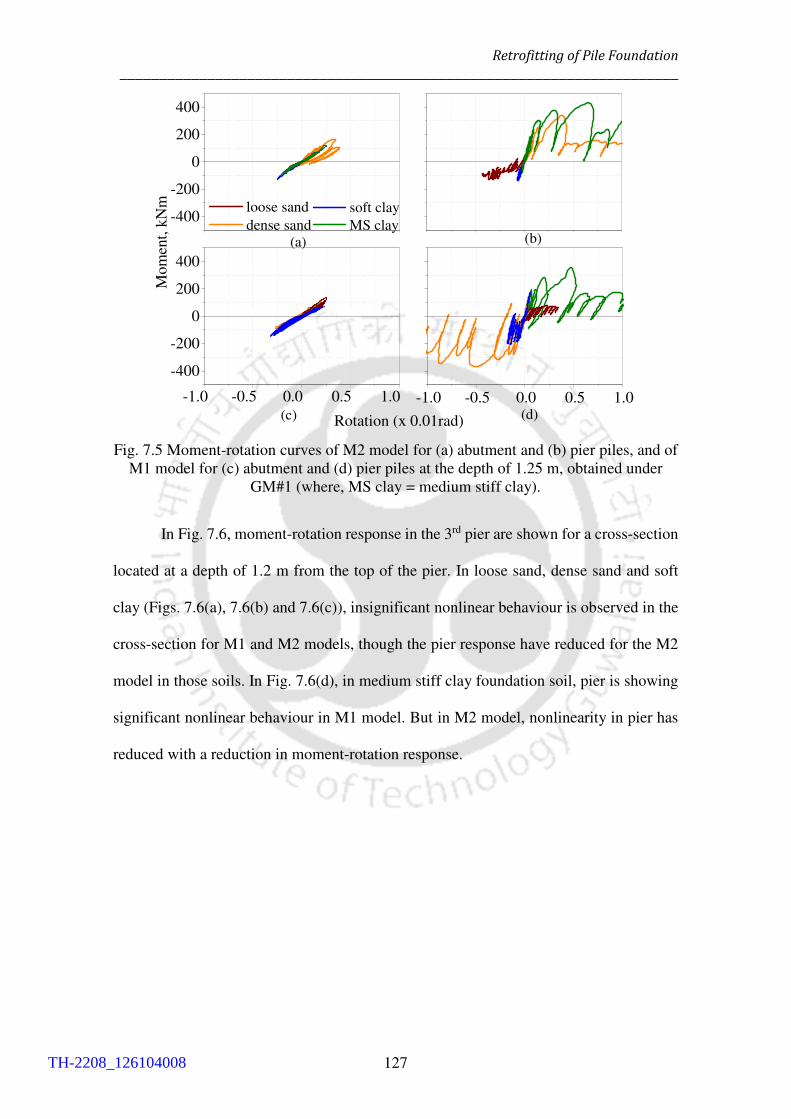
Retrofitting of Pile Foundation
______________________________________________________________________
127
-400
-200
0
200
400
Mom
ent,
kN
m soft clay
MS clay
(c)
(b)
loose sand
dense sand
(a)
-1.0 -0.5 0.0 0.5 1.0
-400
-200
0
200
400
Rotation (x 0.01rad)
-1.0 -0.5 0.0 0.5 1.0(d)
Fig. 7.5 Moment-rotation curves of M2 model for (a) abutment and (b) pier piles, and of
M1 model for (c) abutment and (d) pier piles at the depth of 1.25 m, obtained under
GM#1 (where, MS clay = medium stiff clay).
In Fig. 7.6, moment-rotation response in the 3rd pier are shown for a cross-section
located at a depth of 1.2 m from the top of the pier. In loose sand, dense sand and soft
clay (Figs. 7.6(a), 7.6(b) and 7.6(c)), insignificant nonlinear behaviour is observed in the
cross-section for M1 and M2 models, though the pier response have reduced for the M2
model in those soils. In Fig. 7.6(d), in medium stiff clay foundation soil, pier is showing
significant nonlinear behaviour in M1 model. But in M2 model, nonlinearity in pier has
reduced with a reduction in moment-rotation response.
TH-2208_126104008
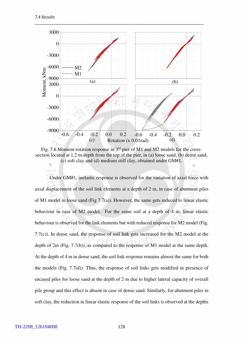
7.4 Results _____________________________________________________________________
128
-9000
-6000
-3000
0
3000
(d)
(b)
(c)
Mom
ent,
kN
m
(a)
-0.6 -0.4 -0.2 0.0 0.2-9000
-6000
-3000
0
3000
Rotation (x 0.01rad)
-0.6 -0.4 -0.2 0.0 0.2
M2
M1
Fig. 7.6 Moment-rotation response in 3rd pier of M1 and M2 models for the cross-
section located at 1.2 m depth from the top of the pier, in (a) loose sand, (b) dense sand,
(c) soft clay and (d) medium stiff clay, obtained under GM#1.
Under GM#1, inelastic response is observed for the variation of axial force with
axial displacement of the soil link elements at a depth of 2 m, in case of abutment piles
of M1 model in loose sand (Fig 7.7(a)). However, the same gets reduced to linear elastic
behaviour in case of M2 model. For the same soil at a depth of 4 m, linear elastic
behaviour is observed for the link elements but with reduced response for M2 model (Fig.
7.7(c)). In dense sand, the response of soil link gets increased for the M2 model at the
depth of 2m (Fig. 7.7(b)), as compared to the response of M1 model at the same depth.
At the depth of 4 m in dense sand, the soil link response remains almost the same for both
the models (Fig. 7.7(d)). Thus, the response of soil links gets modified in presence of
encased piles for loose sand at the depth of 2 m due to higher lateral capacity of overall
pile group and this effect is absent in case of dense sand. Similarly, for abutment piles in
soft clay, the reduction in linear elastic response of the soil links is observed at the depths
TH-2208_126104008

Retrofitting of Pile Foundation
______________________________________________________________________
129
of 2 m and 4 m (Figs. 7.8(a) and 7.8(c)). In case of medium stiff clay, marginal reduction
in the linear axial force - axial displacement response is observed for the soil links at both
the depths (Figs. 7.8(b) and 7.8(d)). Thus, the installation of new encased piles
significantly affects the response of soil with lower lateral stiffness as compared to the
response of soil with higher lateral stiffness.
-200
-100
0
100
200
Ax
ial
Fo
rce,
kN
M1
-0.02 -0.01 0.00 0.01 0.02-50
-25
0
25
50
(c) (d)
(b)
Axial Displacement, m
(a)
-0.002 -0.001 0.000 0.001 0.002
M2
Backbone curve
-0.01 0.00 0.01-25
0
25
50
-0.0015 0.0000 0.0015-20
-10
0
10
20
-0.00025 0.00000 0.00025-50
-25
0
25
50
-0.001 0.000 0.001-200
-100
0
100
200
Fig. 7.7 Variation of axial force with axial displacement of the soil link elements at the
depth of 2 m in (a) loose sand, (b) dense sand, and at the depth of 4 m in (c) loose sand
and (d) dense sand for abutment pile under GM#1.
In Fig. 7.9, the variation of axial force with axial displacement of grout link
elements is shown for different types of foundation soil at the depth of 1 m from the top
of the encased pile. As observed, the grout link elements are subjected to very low axial
strain levels, thus, low-level inelastic behaviour gets mobilized in the grout. The grout is
expected to undergo cracking under very high tensile strain although the deformation of
grout is very minimal in the present study. Among the soils, the maximum and the
minimum response on the compression side are observed for encased piles in soft clay
TH-2208_126104008

7.4 Results _____________________________________________________________________
130
and loose sand respectively. Similar to soil links, grout links have also very negligible
effect on pile behaviour in terms of axial force-deformation. Grout links are modelled in
series with soil links, thus grout and soil link behaviour interact with each other.
-400
-200
0
200
400
Axia
l F
orc
e, k
N
M1
-0.04 -0.02 0.00 0.02 0.04-400
-200
0
200
400
Axial Displacement, m-0.04 -0.02 0.00 0.02 0.04
M2
Backbone curve
-0.0005 0.0000 0.0005
-10
0
10
-0.002 0.000 0.002-60.0
-30.0
0.0
30.0
60.0
-0.001 0.000 0.001-30
0
30
60
-0.0005 0.0000 0.0005
-20
0
20
Fig. 7.8 Variation of axial force with axial displacement for the soil link elements at the
depth of 2 m in (a) soft clay, (b) stiff clay, and at the depth of 4 m in (c) soft clay and
(d) medium stiff clay for abutment pile under GM#1.
Fig. 7.9 Variation of axial force with axial displacement of grout link elements at the
depth of 1 m of encased pile for M2 model (where, MS clay = medium stiff clay).
0.00 0.01 0.02 0.03
0
50
100
150
Lateral Displacement, m
backbone
MS clay
soft clay
dense sand
loose sand
Ax
ial
Fo
rce, k
N
0.000 0.0020
25
50
75
100
TH-2208_126104008

Retrofitting of Pile Foundation
______________________________________________________________________
131
The displacement time histories (DTHs) at the top of 3rd pier (deck-pier junction)
for M1 and M2 models are shown in Fig. 7.10. The residual displacements of M1 model
in loose and dense sand are 0.10 m and 0.097 m, respectively (Fig. 7.10(a)). While in M2
model, the overall deck response gets reduced along with the values of residual
displacements as 0.03 m and 0.075 m in loose sand and dense sand, respectively. A
similar reduction in bridge deck response is observed for M2 model in soft clay and
medium stiff clay as compared to the response of M1 model in the same soils (Fig.
7.10(b)). The M1 model is observed to have peak displacement response of 0.24 m and
0.28 m respectively, and residual response of 0.069 m and 0.15 m respectively in soft clay
and medium stiff clay. For the same soils, the residual displacement response at the deck
level of M2 model get reduced to 0.036 m and 0.10 m, respectively. The reduction in
overall bridge deck response can be primarily attributed to the increased lateral stiffness
of the abutment pile groups as well as that of the bridge through addition of the new
encased piles. That also leads to the improvement of serviceability aspect of the bridge
deck.
0 10 20 30
-0.30
-0.15
0.00
0.15
0.30
M2_dense sand
M1_dense sand
M2_loose sand
M1_loose sand
Dis
pla
cem
ent,
m
0 10 20 30 Time, s (b)
M1_MS clay
M1_soft clay
M2_MS clay
M2_soft clay
(a)
Fig. 7.10 Comparison of DTHs at the top of 3rd pier in (a) loose sand and dense sand,
and (b) medium stiff clay and soft clay, for M1 and M2 models under GM#1 (where,
MS clay = medium stiff clay).
7.4.2 Comparison between M2 and M3 models
Moment-rotation response in 3rd pier of M2 and M3 models for the cross-section located
TH-2208_126104008
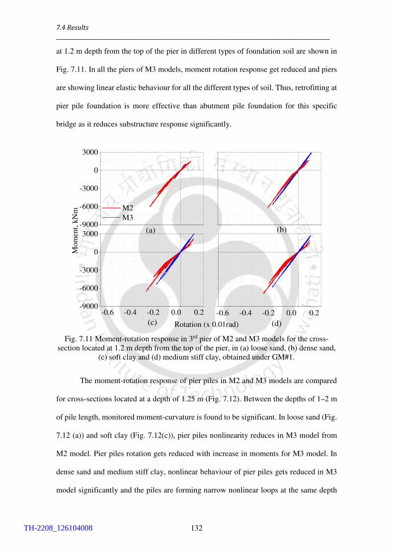
7.4 Results _____________________________________________________________________
132
at 1.2 m depth from the top of the pier in different types of foundation soil are shown in
Fig. 7.11. In all the piers of M3 models, moment rotation response get reduced and piers
are showing linear elastic behaviour for all the different types of soil. Thus, retrofitting at
pier pile foundation is more effective than abutment pile foundation for this specific
bridge as it reduces substructure response significantly.
-9000
-6000
-3000
0
3000
(d)
(b)
(c)
Mom
ent,
kN
m
(a)
-0.6 -0.4 -0.2 0.0 0.2-9000
-6000
-3000
0
3000
Rotation (x 0.01rad)
-0.6 -0.4 -0.2 0.0 0.2
M2
M3
Fig. 7.11 Moment-rotation response in 3rd pier of M2 and M3 models for the cross-
section located at 1.2 m depth from the top of the pier, in (a) loose sand, (b) dense sand,
(c) soft clay and (d) medium stiff clay, obtained under GM#1.
The moment-rotation response of pier piles in M2 and M3 models are compared
for cross-sections located at a depth of 1.25 m (Fig. 7.12). Between the depths of 1–2 m
of pile length, monitored moment-curvature is found to be significant. In loose sand (Fig.
7.12 (a)) and soft clay (Fig. 7.12(c)), pier piles nonlinearity reduces in M3 model from
M2 model. Pier piles rotation gets reduced with increase in moments for M3 model. In
dense sand and medium stiff clay, nonlinear behaviour of pier piles gets reduced in M3
model significantly and the piles are forming narrow nonlinear loops at the same depth
TH-2208_126104008

Retrofitting of Pile Foundation
______________________________________________________________________
133
of 1.25 m (Figs. 7.12(b) and 7.12(d)). For M3 models in different types of foundation
soil, the response of the overall bridge is observed to be significantly reduced specially
in medium stiff clay and dense sand.
For abutment piles in loose sand, linear elastic moment-rotation response is
observed at the depth of 1.25 m from the ground level for M3 model and response has
reduced from M2 model (Fig. 7.13 (a)). For all other soils, moment-rotation response is
observed to be more for M3 models than M2 models at abutment piles (Figs. 7.13 (b),
7.13 (c) and 7.13(d)). So, special attention needs to be taken to achieve linear elastic
response at abutment piles for M3 models.
-400
-200
0
200
400
(d)
(b)
(c)
Mom
ent,
kN
m
(a)
-1.0 -0.5 0.0 0.5 1.0
-400
-200
0
200
400
Rotation (x 0.01rad)
-1.0 -0.5 0.0 0.5 1.0
M2
M3
Fig. 7.12 Comparison of moment-rotation response for pier piles in M2 and M3 models
at a depth of 1.25 m with (a) loose sand, (b) dense sand, (c) soft clay and (d) medium
stiff clay under GM#1.
TH-2208_126104008

7.4 Results _____________________________________________________________________
134
-400
-200
0
200
400
(d)
(b)
(c)
Mom
ent,
kN
m
(a)
-1.0 -0.5 0.0 0.5 1.0
-400
-200
0
200
400
Rotation (x 0.01rad)
-1.0 -0.5 0.0 0.5 1.0
M2
M3
Fig. 7.13 Comparison of moment-rotation response for abutment piles in M2 and M3
models at a depth of 1.25 m with (a) loose sand, (b) dense sand, (c) soft clay and (d)
medium stiff clay under GM#1.
Comparison of the DTHs at bridge deck level for the two models shows the
reduction of deck displacement for stiff clay and dense sand foundation soils (Figs.
7.14(a) and 7.14(b)). The displacement response of M3 model in loose sand and soft clay
are quite similar to that of the M2 model. With the presence of new encased piles at
abutments and pier foundations, there is a significant increase in the lateral stiffness of
the overall bridge that further leads to the observed reduction in bridge deck response. At
deck level, the nonlinear behaviour of the piers has reduced significantly (Fig. 7.11), thus
the displacement of the deck also gets reduced and ends up with insignificant residual
deformation.
TH-2208_126104008
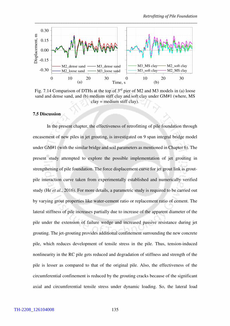
Retrofitting of Pile Foundation
______________________________________________________________________
135
0 10 20 30
-0.30
-0.15
0.00
0.15
0.30
M2_dense sand M3_dense sand
M2_loose sand M3_loose sand
Dis
pla
cem
ent,
m
0 10 20 30 Time, s (b)
M3_MS clay M2_soft clay
M3_soft clay M2_MS clay
(a)
Fig. 7.14 Comparison of DTHs at the top of 3rd pier of M2 and M3 models in (a) loose
sand and dense sand, and (b) medium stiff clay and soft clay under GM#1 (where, MS
clay = medium stiff clay).
7.5 Discussion
In the present chapter, the effectiveness of retrofitting of pile foundation through
encasement of new piles in jet grouting, is investigated on 9 span integral bridge model
under GM#1 (with the similar bridge and soil parameters as mentioned in Chapter 6). The
present study attempted to explore the possible implementation of jet grouting in
strengthening of pile foundation. The force displacement curve for jet grout link is grout-
pile interaction curve taken from experimentally established and numerically verified
study (He et al., 2016). For more details, a parametric study is required to be carried out
by varying grout properties like water-cement ratio or replacement ratio of cement. The
lateral stiffness of pile increases partially due to increase of the apparent diameter of the
pile under the extension of failure wedge and increased passive resistance during jet
grouting. The jet-grouting provides additional confinement surrounding the new concrete
pile, which reduces development of tensile stress in the pile. Thus, tension-induced
nonlinearity in the RC pile gets reduced and degradation of stiffness and strength of the
pile is lesser as compared to that of the original pile. Also, the effectiveness of the
circumferential confinement is reduced by the grouting cracks because of the significant
axial and circumferential tensile stress under dynamic loading. So, the lateral load
TH-2208_126104008

7.5 Discussion _____________________________________________________________________
136
capacity of the encased pile is governed by passive resistance of soil and plastic damage
of jet grouting.
The response of abutment piles are observed to get increased from M1 models to
M3 models in all types of foundation soils except loose sand. However, the response of
the pier piles gets reduced significantly from M2 to M3 models on implementation of the
retrofitting technique. However, for the piers, response has reduced at all retrofitting
stages. More studies need to be carried out regarding the strengthening of abutment piles
for M3 models.
The effectiveness of the first stage of retrofitting (response of the M2 model) is
reflected through the reduction of residual displacement at deck level by 67.1% and
53.2% as compared to the response of M1 model in medium stiff clay and soft clay,
respectively. When further encased piles are added at pier pile foundation, the response
of M3 models get reduced with reduction in deck-level displacement. Also, linear elastic
response is observed in the bridge piers in all types of foundation soils of M3 models as
compared to the nonlinear response of M1 models.
TH-2208_126104008

______________________________________________________________________
Chapter 8
Conclusions and Future Scope of Work
8.1 Conclusions
The significant contribution of the present study involves the comprehensive comparison
of seismic response of an integral bridge on RC pile foundation using the detailed and
simplified modelling approaches for soil-structure interaction. From the results,
significant differences are observed in the response quantities using the two modelling
approaches. Subsequently, the nonlinear behaviours of the substructure and foundation
components of an integral bridge are also investigated by varying the overall length of
the integral bridge model. Finally, with the possibility of extensive seismic damages in
RC pile foundation below such bridge, the applicability of retrofitting of pile foundation
using new encased piles in jet grout, is investigated for the considered 9 span integral
bridge model.
Based on the present study, the following salient conclusions are drawn:
1. Consideration of soil domain and the foundation in the modelling of bridge-
foundation-soil system (in absence of backfill soil) results in reduced overall
response of the system under site specific ground motions, as compared to the
response without the modelling of the soil domain (also in absence of backfill soil).
Under strong earthquake shaking, differential settlement occurs at different location
of bridge foundation. Abutment backfill itself may withstand high deformation and
it reduces the amplification of bridge superstructure by confining it, along the length
of the bridge, from both the ends.
2. The presence of abutment-backfill interaction tends to restrain the bridge deck during
earthquake shaking, leading to a reduction in the displacement response at the deck
level. During strong earthquake shaking, nonlinearity in structural components tends
TH-2208_126104008

8.1 Conclusions
______________________________________________________________________
138
to dominate the seismic response of integral bridge-foundation-soil system.
However, during low intensity of earthquake shaking, nonlinearity of soil tends to
govern the overall system response.
3. The simplified modelling of soil-structure interaction through nonlinear spring-
dashpot system tends to overestimate the bridge-foundation response as compared to
the integral bridge-foundation response obtained by modelling of soil as a
continuum. This is attributed to the higher lateral stiffness and strength of soil as
estimated by the conventionally used API curves (API, 2000) for foundation soil.
The use of spring-dashpot model enhances the response at the deck level and results
in higher forces and moments at pier-deck junctions.
4. In presence of backfill soil, the spring-dashpot modelling approach leads to higher
nonlinear response of integral bridge-foundation system as compared to the response
obtained by adopting the continuum soil model.
5. With increase in the overall length, seismic demand on an integral bridge with RC
pile foundation increases due to the monolithic action of the bridge abutment-deck-
pier system. During strong earthquake shaking, the pile foundation below such long
integral bridge, particularly in clayey soil, is observed to become vulnerable to
failure.
6. Full SSI with BA model shows lesser moment-curvature response compare to FB_SD
with BA model so the overall imposed deformation on the bridge is also less. The
residual deck displacement of FB_SD with BA model is also higher. Which results in
elasto-plastic behaviour in bridge piers. From damping point of view, SSI models
release more seismic energy than the FB_SD models in presence of continuum soil
domain. Bridge piers structural response (moment and shear force) have been upto
10% higher in FB_SD models than full SSI models. So, from a designer point of view,
TH-2208_126104008

Conclusions and Future Scope of Work
______________________________________________________________________
139
if engineers want to predict the piers designing forces from FB_SD models then they
might be over predicting the results by 10% in reality for this specific local site
condition, but, prior to that, proper site investigation analysis needs to be carried out.
7. The retrofitting method of pile foundation in an integral bridge through addition of
new piles encased with jet grout, is found to be more effective for reducing the overall
response of the bridge on medium stiff clayey soil.
8.2 New Contributions of the Present Study
The novelty of the present work is discussed as follows:
1. The seismic response of a multi-span integral bridge-soil system, with RC pile
foundation, is compared with the different modelling approaches considering
simplified and detailed soil-structure interaction aspects, along with site-specific
ground motions. The relative performance of an integral bridge using commonly
adopted spring-dashpot soil model with that of an integral bridge using detailed
continuum soil model is investigated (absent in past studies).
2. The influence of overall length of an integral bridge-foundation-soil system on its
response due to temperature loading, has been investigated in the past studies.
However, the variation in seismic response of such an integral bridge-foundation-
soil system with overall length, is attempted for the first time.
3. Effectiveness of seismic retrofitting of RC pile foundation below an integral bridge,
using new piles encased in jet grout, is studied through numerical modelling of the
bridge-pile-soil system. Past studies have carried out practical implementations of
different methods, but the numerical modelling and analysis were absent for the
different methods.
TH-2208_126104008

8.3 Scope of Future Work
______________________________________________________________________
140
8.3 Scope of Future Work
1. The comparative seismic response of bridge-soil system using different modelling
approaches can be studied for other types of bridges with bearings or shear keys.
Particularly, the relative performances of bridge-soil system with spring-dashpot
modelling and soil continuum modelling, under nonlinear time history analysis,
need to be investigated.
2. The retrofitting method of pile foundation using new piles encased in jet grout,
needs to be investigated in more detail for intermediate pier pile foundation in
integral and other types of bridges. Detailed parametric study needs to be carried
out by varying different bridge-specific parameters.
3. Further studies need to be conducted on the influence of ground motion parameters
on the seismic response of an integral bridge-soil system, to identify the salient
factors responsible for seismic vulnerability of such bridges.
4. API (2000) guidelines need reconsideration as it over predict the soil strength under
dynamic analysis, which effects structural nonlinearities too. Correspondingly,
foundation design should be rechecked if it’s founded on softer soil and excess pore
water pressure dissipation needs to be considered. Because over predicting
foundation strength can be detrimental to overall bridge.
5. In case, the foundation soil is comparatively soft (mainly, sands) and soil
liquefaction appears to be a major problem then it’s better to consider interface
elements to capture SSI in a more accurate manner. Because the present study is
only limited to drained (or dry) condition of soil.
6. In the present study, varying the span length with no. of span of an integral bridge
can be done in future to optimize the span length. With that, pier and pile
configuration need to be arranged accordingly to complete the study.
TH-2208_126104008

______________________________________________________________________
References
AASHTO. (1989). Guide Specifications - Thermal Effects in Concrete Bridge Superstructures.
Washington, DC: American Association of State Highway and Transportation Officials.
AASHTO. (1996). Standard Specifications for Highway Bridges (16th ed.).Washington DC:
American Association of State Highway and Transportation Officials.
AASHTO. (2002). Standard Specifications for Highway Bridges (17th ed.). Washington DC:
American Association of State Highway and Transportation Officials.
AASHTO LRFD. (2012). Bridge Design Specifications (6th ed.). Washington, DC: American
Association of State Highway and Transportation Officials.
Abendroth, R.E., & Greimann, L.F. (1988). Rational design approach for integral abutment piles.
Transportation Research Record, 1233.
Abendroth, R. E., & Greimann, L. F. (2005). Field testing of integral abutments. Final Rep. HR-
399, Iowa State University, Ames, IA.
Abendroth, R.E., Greimann, L.F., & Ebner, P.B. (1989). Abutment pile design for jointless
bridges. Journal of Structural Engineering, 115, 2914–2929.
Abendroth, R. E., Greimann, L. F., & LaViolette, M. D. (2007). An integral abutment bridge with
precast concrete piles. Iowa Department of Transportation, CTRE Project 99-48.
ACI. (1982). Prediction of creep, shrinkage, and temperature effects in concrete structures. American Concrete Institute, Tech. Rep. ACI 209R-82, Detroit, MI.
ADINA. (2017). Automatic Dynamic Incremental Nonlinear Analysis. ADINA R & D, Inc.,
Watertown, MA, www.adina.com. AISC (1996). Steel Construction Manual. California: American Institute of Steel Construction.
Inc., 13th edition, 1st print.
Anderson, D.G., Martin, G.R., Lam, I., & Wang, J.N. (2008). Seismic analysis and design of
retaining walls, buried structures, slopes and embankments. National Cooperative Highway Research Program, NCHRP Report 611, Transportation Research Board, Washington, DC.
ANSYS. (2013). Mechanical APDL Introductory Tutorials, Release 15.0. ANSYS, Inc., PA,
USA.
API RP2A-WSD. (2000). Recommended practice for planning, designing and constructing fixed
offshore platforms-working stress design. American Petroleum Institute, 2000, Washington
D.C, USA.
Argyroudis, S., Palaiochorinou, A., Mitoulis, S., & Pitilakis, D. (2016). Use of rubberised
backfills for improving the seismic response of integral abutment bridges. Bulletin of Earthquake Engineering, 14, 3573-3590.
Arockiasamy, M., Butrieng, N., & Sivakumar, M. (2004). State-of-the-art of integral abutment
bridges: Design and practice. Journal of Bridge Engineering, 9, 497–506.
Arockiasamy. M., & Sivakumar, M. (2005). Effects of restraint moments in integral abutment
bridges. The 2005FHWA Conference, Integral Abutment and Jointless Bridges (IAJB2005) (pp. 185–198). Baltimore, MD.
Arsoy, S., Richard, M.B., & Duncan, J.M. (1999). The behaviour of integral abutment bridges. Virginia Tech. Research Counsel, VTRC 00-CR3, Blacksberg, VA.
Arsoy, S., Barker, R.M., & Duncan, M.J. (2002). Experimental and analytical investigations of the piles and abutments of integral bridges. Virginia Tech. Research Counsel, FHWA/NTRC
02-CR6, Charlottesville, VA.
Austroads. (2004). Guide to the structural design of road pavements. Austroads: Sydney,
Australia.
BA 42/96 Amendment No. 1. (2003). Design Manual for Integral Bridges: Design Manual for Road and Bridges. Volume 1, Section 3, Part 12. The Highway Agency, UK.
Badoni, D., & Makris, N. (1996). Nonlinear response of single piles under lateral inertial and
seismic loads. Soil Dynamics and Earthquake Engineering, 15(1), 29–43.
Bahjat, R. (2014). Short and Long-term Performance of a Skewed Integral Abutment Prestressed Concrete Bridge, Master’s Thesis. University of Massachusetts, Amherst, MA.
TH-2208_126104008
�����������______________________________________________________________________
142
Baptiste, K.T., Kim, W., & Laman, J.A. (2011). Parametric study and length limitations for
prestressed concrete girders integral abutment bridges. Structural Engineering International, 21, 151–156.
Barker, K.J., & Carder, D.R. (2001). Performance of an integral bridge over the m1- a1 link road
at Bramham crossroads. Transport Research Laboratory, TRL Project Report 521, UK.
Barker, R.M., Duncan, J.M., Rojiani, K.B., Ooi, P.S.K., Tan, C.K., & Kim, S.G. (1991). Manual
for the Design of Bridge Foundations. National Cooperative Highway Research Program, NCHRP Report 343, Transportation Research Board, Washington, DC.
Barr, P. J., Halling, M. W., Huffaker, C., & Boyle, H. (2013). Behaviour and analysis of an
integral abutment bridge. Department of Civil and Environmental Engineering, Utah State University, Utah.
Bazant, Z.P., & Panula, L. (1980). Creep and shrinkage characterization for analysing prestressed
concrete structures. PCI Journal, 86–121.
Bonczar, C., Brena, S., Civijan, S., DeJong, J., & Crovo, D. (2005). Integral abutment pile
behaviour and design-field data and fem studies. The 2005FHWA Conference, Integral Abutment and Jointless Bridges (IAJB 2005), Baltimore, MD.
Boulanger, R.W., Curras, C.J., Kutter, B.L., Wilson, D.W., & Abghari, A. (1999). Seismic soil-
pile-structure interaction experiments and analysis. Jr. of Geotech. Engg. ASCE, 125(9): 750-
759.
Brødbæk, K.T., Møller, M., Sørensen, S.P.H., & Augustesen, A.H. (2009). Review of p-y
relationships in cohesionless soil. Aalborg: Department of Civil Engineering, Aalborg University, DCE Technical Reports; No. 57.
Breña, S. F., Bonczar, C. H., Civjan, S. A., DeJong, J. T., & Crovo, D. S. (2007). Evaluation of
seasonal and yearly behavior of an integral abutment bridge. Journal of Bridge Engineering,
12, 296-305.
Briseghella, B., & Zordan, T. (2015). An innovative steel-concrete joint for integral abutment
bridges. Journal of Traffic and Transportation Engineering (English Edition), 2, 209-222.
Broms, B. B. (1964). Lateral Resistance of Piles in Cohesive Soils. In Proceedings of the American Society of Civil Engineers, Journal of the Soil Mechanics and Foundations Division,
90, SM2.
BSDC. (2017). Bridge Structures Design Criteria. Technical Standard Branch, Alberta
Transportation, Canada.
BSI. (1998). Steel, concrete, and composite bridges. British Standard Institution, BS 5400-1:
London, UK.
Burdette, E. G., Tidwell, J. B., Ingram, E. E., Goodpasture, D. W., Howard, S. C., Wasserman,
E. P., and Deatherage, J. H. (2004). Lateral load tests on prestressed concrete piles supporting
integral abutments. PCI Journal, 495, 70–77.
Burke, M.P.J. (1993). Integral bridges: attributes and limitations. Transportation Research Record, 1393.
Burke, M. P. J. (2009). Integral and semi-integral bridges. John Wiley & Sons.
Caltrans. (2004). Seismic design criteria. Version 1.3, California Department of Transportation,
CA.
Caltrans. (2013). Seismic design criteria, California Department of Transportation Version 1.7.
CFEM. (2006). Canadian Foundation Engineering Manual, 4th edition. Canadian Geotechnical
Society, Toronto, Canada.
Mander, J.B., Priestley, M.J.N. & Park R. (1984). Theoretical Stress-Strain Model for Confined
Concrete. Journal of Structural Engineering, 114(3):1804-1826
Lopez-Caballero, F., Régnier, J., Bonilla, F. & Gélis, C. (2011). Site response analysis including
earthquake input ground motion and soil dynamic properties variability. In: Proceedings of the 15th World Conference on Earthquake Engineering, Lisbon, Portugal.
CHBDC. (2014). Canadian Highway Bridge Design Code. Canadian Standards Association,
CAN/CSA S6-14, Canada.
Chuhan, Z., Yanjie, X. & Feng, J. (1998) Effects of soil-structure interaction on nonlinear
response of arch dams, Developments in Geotech Eng, 83:95-114, ISSN 0165-1250,
http://dx.doi.org/10.1016/S0165-1250(98)80006-0.
TH-2208_126104008

����������� ______________________________________________________________________
143
Chung, Y. S., Park, C. K., & Lee, D. H. (2006). Seismic performance of RC bridge piers subjected
to moderate earthquakes. Structural Engineering and Mechanics, 24(4), 429-446.
Civjan, S. A., Bonczar, C., Brena, S. F., DeJong, J., & Crovo, D. (2007). Integral abutment bridge
behavior: Parametric analysis of a Massachusetts bridge. Journal of Bridge Engineering,
12(1), 64-71.
Civjan, S. A., Kalayci, E., Quinn, B. H., Breña, S. F., & Allen, C. A. (2013). Observed integral
abutment bridge substructure response. Engineering Structures, 56, 1177-1191.
Claugh, G.M., & Duncan, J.M. (1991). Foundation engineering handbook, Indian edition edn.
CBS publisheres, New Delhi, India.
Comisu, C. C. (2005). Integral Abutment and Jointless Bridges. The Bulletin of the Polytechnic Institute of Jassy, Construction. Architecture Section, 51, 107-117.
Conboy, D., & Stoothoff, E. (2005) Integral abutment design and construction: The New England
experience. The 2005FHWA Conference, Integral Abutment and Jointless Bridges (IAJB 2005) (pp. 50-60). Baltimore, Maryland.
Connal, J. (2004). Integral Abutment Bridges–Australian and US Practice. In 5th Austroads bridge conference, Hobart, Tasmania.
CSI. (2016). Introduction to CSiBRIDGE, v. 17. Computers and Structures, USA.
CSI. (2017). Introduction to SAP2000, v. 19.2.1. Computers and Structures, USA.
Cui, L., & Mitoulis, S. (2015). DEM analysis of green rubberised backfills towards future smart
Integral Abutment Bridges (IABs). Geomechanics from Micro to Macro, Vols I and II, 583-
588.
Darendeli, M.B. (2001). Development of a new family of normalized modulus reduction and material damping curves. Ph.D Thesis, University of Texas. Austin, Texas.
Darley, P., & Alderman, G.H. (1995). Measurement of thermal cyclic movements on two portal
frame bridges on the m1. Transport Research Laboratory, TRL Project Report 165, UK.
Darley, P., Carder, D.R., & Barker, K.J. (1998). Seasonal thermal effects over three years on the
shallow abutment of an integral bridge in Glasgow. Transport Research Laboratory, TRL
Project Report 344, UK.
DeLano, J.G. (2002). Behaviour of pile-supported integral abutments at bridge sites with shallow bedrock. Master’s thesis, Department of Civil Engineering, University of Maine.
Deng, Y., Phares, B. M., Greimann, L., Shryack, G. L., & Hoffman, J. J. (2015). Behavior of
curved and skewed bridges with integral abutments. Journal of Constructional Steel Research,
109, 115-136.
Dhar, S., �zcebe, A.G., Dasgupta, K., Dey, A., Paolucci, R. & Petrini, L. (2016). Nonlinear
Dynamic Soil-Structure Interaction Effects on the Seismic Response of a Pile-Supported
Integral Bridge Structure. In 6th International Conference on Recent Advances in Geotechnical Earthquake Engineering and Soil Dynamics. Paper No. 141, New Delhi, India.
Dicleli, M. (2000). Simplified model for computer-aided analysis of integral bridges. Journal of Bridge Engineering, 5, 240–248.
Dicleli, M., & Albhaisi, S.M. (2003). Maximum length of integral bridges supported on steel h-
piles driven in sand. Engineering Structures, 25, 1491–1504.
Dicleli, M., & Albhaisi, S.M. (2004). Performance of abutment-backfill system under thermal
variations in integral bridge built in clay. Engineering Structures, 26, 949–962.
Douglas, B.M., & Reid, W.H. (1982). Dynamic test and system identification of bridges. Journal of structural division, 108, 2295–2312.
Duncan, J.M., & Arsoy, S. (2003). Effect of bridge-soil interaction on behaviour of piles
supporting integral bridges. Transportation Research Record, 1849.
Duncan, M.J., & Mokwa, R.L. (2001). Passive earth pressure: Theories and tests. Journal of Geotechnical and Geoenvironmental Engineering, 127, 248–257.
Dunker, K. F., & Liu, D. (2007). Foundations for integral abutments. Practice Periodical on Structural Design and Construction, 12(1), 22-30.
Dutta, T.K. (2010). Seismic Analysis of Structures. John Wiley & Sons (Asia) Pte Ltd.
Efretuei, E. O. (2013). Thermal impact on soil-structure interaction for integral bridges (PhD
dissertation). School of Civil Engineering, University of Leeds, UK.
TH-2208_126104008

�����������______________________________________________________________________
144
Elgamal, A., Yan, L., Yang, Z., & Conte, J.P. (2008). Three-dimensional seismic response of
Humboldt bridge-foundation-ground system. Journal of Structural Engineering, 134, 1165–
1176.
Emerson, M. (1976). Bridge temperatures estimated from the shade temperature. Transportation Research Record, TLR Project Report 696, Transport and Road Research Laboratory, UK.
EN 1998-2. (2005). Eurocode 8: Design of structures for earthquake resistance. Part 2: Bridges.
Brussels, Belgium.
England, G.L., Tsang, N.C.M., & Bush, D.L. (2000). Integral Bridges: A Fundamental Approach to the Time-Temperature Loading Problem. Thomas Telford Ltd. UK.
Erhan, S., & Dicleli, M. (2017). Parametric study on the effect of structural and geotechnical
properties on the seismic performance of integral bridges. Bulletin of Earthquake Engineering,
15(10), 4163-4191.
Fan, C.C, & Long, J.H. (2005). Assessment of existing methods for predicting soil responses of
laterally loaded piles in sand. Computers and Geotechnics, 32,274–289.
Far, N. E., Maleki, S., & Barghian, M. (2015). Design of integral abutment bridges for combined
thermal and seismic loads. Earthquakes and Structures, 9, 415-430.
Faraji, S., Ting, J.M., Crovo, D.S., & Ernst, H. (2001). Nonlinear analysis of integral bridges:
finite element model. Journal of Geotechnical and Geoenvironrnental Engineering, 127, 454–
461.
Figini, R & Paolucci, R. (2017). Integrated foundation–structure seismic assessment through non-
linear dynamic analyses. Earthquake Eng & Struct. Dyn., 46(3), 349-367. 10.1002/eqe.2790. Fleming, W. G. K., Weltman, A. J., Randolph, M. F., & Elson, W. K. (1992). Piling Engineering.
Blackie Academic & Professional, Glasgow, UK.
Filippou, F.C., Popov, E.P. & Bertero, V.V. (1983). Effects of Bond Deterioration on Hysteretic
Behavior of Reinforced Concrete Joints. Earthquake Engineering Research Center, Report
EERC 83-19, University of California, Berkeley.
Frangi, A., Collin, P., & Geier, R. (2011). Bridges with Integral Abutments: Introduction.
Structural Engineering International, 21, 144-150.
Frosch, R.J., Wenning, M., & Chovichien, V. (2005). The in-service behavior of integral
abutment bridges: abutment-pile response. The 2005FHWA Conference, Integral Abutment and Jointless Bridges (IAJB 2005) (pp. 270-280). Baltimore, MD.
Fukada, H., Kato, K., Aoyagi, M., Inagawa, H., & Shioi, Y. (2005). Application of reinforcing
methods for existing pile foundation on soft ground (in-cap method). In Public Works Research Institute: The 23th US-Japan Bridge Engineering Workshop. Retrieved July (Vol. 1,
p. 2014).
Gazetas, G. (1991), Formulas and charts for impedances of surface and embedded foundations.
Jr. of Geotech. Eng. 117(9), 1363-81.
Gazetas, G., & Dobry, R. (1984). Horizontal response of piles in layered soils. Journal of Geotechnical Engineering, 110(1), 20–40.
Gentela, S.R., & Dasgupta, K. (2012). Influence of soil-structure interaction on seismic design of
reinforced concrete integral bridges. In: Proceedings of the International Symposium on Engineering under Uncertainty: Safety Assessment ad Management (ISEUSAM-2012) (pp.
743–756). Kolkata: Springer.
Gibbens, B., & McManus, A. (2011). Design of Peninsula Link Integral Bridges. In Austroads Bridge Conference, Sydney.
Girton, D.D., Hawkinson, T.R., & Greimann, L.F. (1991). Validation of design recommendations
for integral-abutment piles. Journal of Structural Engineering, 117, 2117–2134. Granas, J.L. (2016). Undrained lateral soil response of offshore monopile in layered soil. M.Tech Thesis,
Dept. of Civ. & Transport Eng., NTNU.
Greimann, L.F., & Wolde-Tinsae, A.M. (1988). Design model for piles in jointless bridges.
Journal of Structural Engineering, 114, 1355–1369.
Greimann, L. F., Wolde-Tinsae, A. M., & Yang, P. S. (1983). Skewed bridges with integral
abutments. Transportation Research Record, 903.
TH-2208_126104008

����������� ______________________________________________________________________
145
Greimann, L. F., Yang, P. S., Edmunds, S. K., & Wolde-Tinsae, A. M. (1984). Design of Piles
for Integral Abutment Bridges: Final Report. Department of Civil Engineering, Engineering Research Institute, Iowa State University.
Greimann, L.F., Yang, P.S., & Wolde-Tinsae, A.M. (1986). Nonlinear analysis of integral
abutment bridges. Journal of Structural Engineering, 112, 2263–2280.
Greimann, L.F., Abendroth, R.E., Johnson, D.E., & Ebner, P.B. (1987). Pile design and tests for
integral abutment bridges: Final report. Iowa State University, Iowa Department of Transportation, No. Iowa DOT Proj. HR-273.
Hansen, J. B. (1963). Discussion on Hyperbolic Stress-Strain Response, Cohesive Soils. Journal for Soil Mechanics and Foundation Engineering, 89, 241- 242.
Hashash, Y.M.A., Musgrove, M.I., Harmon, J.A., Groholski, D.R., Phillips, C.A., & Park, D.
(2016). DEEPSOIL 6.1, User Manual. Urbana, IL, Board of Trustees of University of Illinois
at Urbana-Champaign
Hassiotis, S., Lopez, J.A., & Bermudez, R. (2005). Full scale testing of an integral abutment
bridge. The 2005FHWA Conference, Integral Abutment and Jointless Bridges (IAJB 2005). Baltimore, MD.
Hassiotis, S., Khodair, Y., Roman, E., & Dehne, Y. (2006). Evaluation of integral abutments.
New Jersey Department of Transportation and U.S. Department of Transportation, Federal Highway Administration. No. FHWA-NJ-2005-025.
He, B., Wang, L., & Hong, Y. (2016). Capacity and failure mechanism of laterally loaded jet-
grouting reinforced piles: Field and numerical investigation. Science China Technological Sciences, 59(5), 763-776.
Hibbitt, D., Karlsson, B., & Sorensen, P. (2014). ABAQUS/CAE Standard User’s Manual (Version 6.14). Pawtucket, RI.: Hibbitt, Karlsson & Sorensen.
Holzer, T.L., Padovani, A.C., Bennett, M.J., Noce, E.T., Tinsley, J.C. (2005). Mapping NEHRP
VS30 Site Classes. Eq. Spectra, 21(2), 1-18.
Horvath, J. S. (2000). Integral-abutment bridges: problems and innovative solutions using EPS
geofoam and other geosynthetics. Manhattan College, School of Engineering, Research
Report No. CE/GE-00, 2, NY.
Horvath, J. S. (2005). Integral-abutment bridges: Geotechnical problems and solutions using
geosynthetics and ground improvement. The 2005FHWA Conference, Integral Abutment and Jointless Bridges (IAJB 2005) (pp. 281-291). Baltimore, MD.
Huang, J., Shield, C. K., & French, C. E. (2008). Parametric study of concrete integral abutment
bridges. Journal of Bridge Engineering, 13, 511-526.
Huckabee, P. (2005). Plastic design of steel HP-piles for integral abutment bridges. The 2005FHWA Conference, Integral Abutment and Jointless Bridges (IAJB 2005) (pp. 270-280).
Baltimore, MD.
Husain, I., & Bagnariol, D. (2000). Design and performance of jointless bridges in Ontario: new
technical and material concepts. Transportation Research Record: Journal of the Transportation Research Board, 1696, 109-121.
Hutchinson, T. C., Chai, Y. H., Boulanger, R. W., & Idriss, I. M. (2004). Inelastic seismic
response of extended pile-shaft-supported bridge structures. Earthquake Spectra, 20(4), 1057-
1080.
IDOT. (2006). Bridge design manual. Iowa Department of Transportation, Ames, IA.
Imbsen, R.A., Vandershaf, D.E., Schamber, R.A., & Nutt, R.V. (1985). Thermal effects in
concrete bridge superstructures, National Cooperative Highway Research Program, NCHRP
Report 276, Transportation Research Board, Washington, DC.
Ingram, E.E., Burdette, E.G., Goodpasture, D.W., & Deatherage, J.H. (2003). Evaluation of
applicability of typical column design equations to steel h-piles supporting integral abutments.
AISC Engineering Journal, 40(1), 50–58.
IRC: 6. (2010). Standard Specifications and code of practice for road bridge. Section:II Load and
Stresses (4th Rev.). New Delhi, IN.: The Indian Roads Congress.
IRC: 112 (2011). Code of Practice for Concrete Road Bridges. New Delhi, IN.: The Indian Roads
Congress.
TH-2208_126104008

�����������______________________________________________________________________
146
Itani, A. M., & Pekcan, G. (2011). Seismic performance of steel plate girder bridges with integral
abutments. U.S. Department of Transportation, Federal Highway Administration. Report No.
FHWA-HIF-11-043.
Jamieson, G. (2009). Towards practical modeling of integral-abutment bridges under longitudinal
load. In 7th Austroads Bridge Conference, Auckland, New Zealand.
JSCE. (1985). Dynamic Analysis and Earthquake Resistant Design. Japanese Society of Civil
Engineers; Vol. 2, Methods of Dynamic Analysis, Oxford and IBH Publishing Co. Pvt. Ltd.
JRA. (2012). Specifications for Highway Bridges. Part V: Seismic Design. Japan Road
Association: Tokyo, Japan.
Jayaraman, R., Merz, P. B., & McLellan. (2001). Integral bridge concept applied to rehabilitate
an existing bridge and construct a dual-use bridge. In 26 th Conference on our World in Concrete and Structures (pp. 26-28).
Jorgenson, J.L. (1983). Behaviour of abutment piles in an integral abutment in response to bridge
movements. Transportation Research Record, 903.
Kagawa, T., & Kraft, L.M, (1980a). Seismic p-y response of flexible piles. Journal of the Geotechnical Engineering, 106, 899–918.
Kagawa, T., & Kraft, L.M. (1980b). Lateral load-deflection relationship of piles subjected to
dynamic loadings. Soils and Foundations, 20, 19–36.
Kamel, M. R., Benak, J. V., Tadros, M. K., & Jamshidi, M. (1996). Prestressed concrete piles in
jointless bridges. PCI Journal, 41, 56–67.
Kausel, E., & Tassoulas, J. L. (1981). Transmitting boundaries: a closed-form comparison.
Bulletin of the seismological society of America, 71(1), 143-159.
Kerokoski, O., & Laaksonen, A. (2005). Soil-structure interaction of jointless bridges. The 2005FHWA Conference, Integral Abutment and Jointless Bridges (IAJB 2005) (pp. 323-336).
Baltimore, MD.
Khalili-Tehrani, P., Shamsabadi, A., Stewart, J. P., & Taciroglu, E. (2016). Backbone curves with
physical parameters for passive lateral response of homogeneous abutment backfills. Bulletin of Earthquake Engineering, 14, 3003-3023.
Khodabakhshi, P., Jahankhah, H., & Ghannad, M. A. (2011). A discrete model for response
estimation of soil-structure systems with embedded foundations. Earthquake Engineering and Engineering Vibration, 10(2), 263-276.
Knickerbocker, D., Basu, P.K., & Wasserman, E.P. (2005). Behavior of two-span integral bridges
unsymmetrical about the pier line. The 2005FHWA Conference, Integral Abutment and Jointless Bridges (IAJB 2005) (pp. 244–256). Baltimore, MD.
Kong, B., Cai, C. S., & Zhang, Y. (2016). Parametric study of an integral abutment bridge
supported by prestressed precast concrete piles. Engineering Structures, 120, 37-48.
Kolay, C. (2009). Seismic analysis of bridge abutment soil system. Master’s thesis. Department
of Civil Engineering, IIT Kanpur, India.
Kontoe, S. (2006). Development of time integration schemes and advanced boundary conditions for dynamic geotechnical analysis (PhD dissertation). Imperial College London. England.
Kontoe, S., Zdravkovi�, L., Potts, D.M., Salandy, N.E. (2007). The Domain Reduction Method
as an advanced boundary condition. In: 4th International Conference on Earthquake Geotechnical Engineering. Paper No. 1231. Greece.
Kramer, S. L. (1996). Geotechnical Earthquake Engineering Prentice Hall. New York.
Kumar, P.V. (2008.) Behaviour of integral abutment bridges under temperature effect and seismic excavation (PhD dissertation). Department of Civil Engineering, Indian Institute of
Technology, Roorkee, India.
Lam, I. P., & Martin, G. R. (1986). Seismic design of highway bridge foundations. volume 2 and
3.
Laman, J.A., & Kim, W. (2010). Integral abutment bridge response under thermal loading.
Engineering Structures, 32, 1495–1508.
Lampe, N., & Azizinamini, A. (2000). Steel bridge system, simple for dead load and continuous
for live load. Conference of High Performance Steel Bridge, Baltimore,MD.
TH-2208_126104008

����������� ______________________________________________________________________
147
Lan, C. (2012). On the performance of super-long integral abutment bridges-parametric analysis and design optimization (PhD dissertation). Engineering of Civil and Mechanical structural
Systems, University of Trento, Italy.
Lawver, A., French, F., & Shield, C.K. (2000). Field performance of an integral abutment bridge.
Transportation Research Record 1740.
Li, Z. N., Li, Q. S., & Lou, M. L. (2005). Numerical studies on the effects of the lateral boundary
on soil-structure interaction in homogeneous soil foundations. Structural Engineering and Mechanics, 20(4), 421-434.
Liu, D., Magliola, R.A., & Dunker, K.F. (2005). Integral abutment bridges: IOWA and Colorado
experience. The 2005FHWA Conference, Integral Abutment and Jointless Bridges (IAJB 2005) (pp. 136–147). Baltimore, MD.
Lu, J., Elgamal, A., & Yang, Z. (2011). OpenSeesPL: 3D Lateral Pile-Ground Interaction User Manual (Beta 1.0). Department of Structural Engineering, University of California, San
Diego, CA.
LUSAS– Finite Element Analysis, (2014). LUSAS User Manual, Version 15.2.
Lysmer, J. & Kuhlemeyer, R.L. (1969). Finite dynamic model for infinite media. J. Eng. Mech. Div. ASCE, 95(EM4), 859-877.
Maberry, J., & Camp, J.B. (2005). New York State Department of Transportation’s experience
with integral abutment bridges. The 2005FHWA Conference, Integral Abutment and Jointless Bridges (IAJB 2005) (pp. 125–135). Baltimore, MD.
Makris, N. & Gazetas, G. (1992), Dynamic pile-soil-pile interaction. Part II: Lateral and seismic
response. Earthquake Engng. Struct. Dyn., 21, 145–162.
Maruri, R.F., & Petro, H. (2005). Integral abutments and jointless bridges (IAJB) 2004 survey
summary. The 2005-FHWA Conference, Integral Abutment and Jointless Bridges (IAJB 2005) (pp. 12-29). Baltimore, MD.
Matlock, H. (1970). Correlations for designs for laterally loaded piles in soft clay. Second Annual
Offshore Technology Conference, Houston, TX.
Matthewson, M.B., Wood, J.H., & Berrill, J.B. (1980). Seismic design of bridges: section 9: Earth
retaining structures. Bulletin of the New Zealand National Society for Earthquake Engineering, 13, 280-293.
Mazzoni, S., McKenna, F., Scott, H.M. & Fenves, G.L. (2007). The OpenSees Command Language Manual, v6.0. Pacific Earthquake Engineering Research Center, University of
California, Berkeley. http://opensees.berkeley.edu
McBride, K. C. (2005). Thermal Stresses in the Superstructure of Integral Abutment Bridges. West Virginia University Libraries, VA.
McClelland, B., & Focht, J.A. (1958). Soil modulus of laterally loaded piles. Transactions of the American Society of Civil Engineers, 123(1), 1049-1063.
McKenna, F. & Fenves, G.L. (2008). Using the OpenSees interpreter in Parallel Computers.
University of California, Berkeley. NEESit; TN-2007-16, v1.0 MIDAS Civil. (2017). Design of Civil Structures: Integrated Solution System for Bridge and Civil
Engineering. v2.1.
Mistry, V. (2005). Integral abutment and jointless bridges. In The 2005-FHWA Conference, Integral Abutment and Jointless Bridges (IAJB 2005) (pp. 3-11). Baltimore, MD.
Mitoulis, S. A. (2016). Some open issues in the seismic design of bridges to Eurocode 8-2.
Challenge Journal of Structural Mechanics, 2(1), 7-13.
Mitoulis, S., Argyroudis, S., & Kowalsky, M. (2015). Evaluation of the stiffness and damping of
abutments to extend direct displacement based design to the design of integral bridges. In
Proceedings of the Computational Methods in Structural Dynamics and Earthquake Engineering, Crete,Greece.
Mitoulis, S. A., Palaiochorinou, A., Georgiadis, I., & Argyroudis, S. (2016). Extending the
application of integral frame abutment bridges in earthquake�prone areas by using novel
isolators of recycled materials. Earthquake Engineering & Structural Dynamics, 45, 2283-
2301.
TH-2208_126104008

�����������______________________________________________________________________
148
Mokwa, R. L. (1999). Investigation of the resistance of pile caps to lateral spreading (PhD
dissertation). Dept. of Civil Engineering, Virginia. Polytechnic Institute and State Univ.,
Blacksburg, Va.
Mokwa, R.L. & Duncan, J.M. (2000). Investigation of the Resistance of Pile Caps and Integral
Abutments to Lateral Loading. Final Contract Report. Virginia Transportation Research Council, Virginia Tech, Blacksburg, VA.
Monkul, M.M. (2008). Validation of Practice Oriented Models and Influence of Soil Stiffness on
Lateral Pile Response Due to Kinematic Loading. Marine Geores. & Geotech, 26(3), 145-159.
Mourad, S., & Tabsh, S.W. (1998). Pile forces in integral abutment bridges subjected to truck
loads. Transportation Research Record, 1633, 77-83.
Murchison, J.M. (1983). An evaluation of p-y relationships in sands. American Petroleum Institute (API), Research Report 41, USA.
Nielsen, R.J. & Schmeckpeper, E.R. (2001). Consistent Design of Integral Abutment, Bridges.
Department of Civil Engineering, University of Idaho, Moscow, Idaho.
Novak, M., & Sheta, M. (1980). Approximate approach to contact effects of piles. In: Proceedings on Session of Dynamic Response of Pile Foundations: Analysis Aspects (pp. 53–79), ASCE.
NZTA. (2014). Bridge manual, (SP/M/022). New Zealand Transportation Authority, 3rd edition,
amendment 1. Wellington: NZ Transport Agency.
Olson, S. M., Holloway, K. P., Buenker, J. M., Long, J. H., & LaFave, J. M. (2013). Thermal
behavior of IDOT integral abutment bridges and proposed design modifications. University of Illinois Urbana Champaign, Illinois Department of Transportation, FHWA-ICT -12- 022.
Paraschos, A. (2016). Effects of Wingwall Configurations on the Behaviour of Integral Abutment Bridges (PhD dissertation). Department of Civil & Environmental Engineering, University of
Maryland, MD.
Perkun, J., & Michael, K. (2005). Design and construction of dual 630-foot, jointless, three-span
continuous multi-girder bridges in St. Albans, West Virginia, United States, carrying U.S.
route 60 over the coal river. In The 2005FHWA Conference, Integral Abutment and Jointless Bridges (IAJB 2005) (pp. 97-112). Baltimore, MD.
Petursson, K., & Kerokoski, P. (2011). Monitoring and analysis of abutment-soil interaction of
two integral bridges. Journal of Bridge Engineering, 18(1), 54–64.
Phares, B. M., Faris, A. S., Greimann, L., & Bierwagen, D. (2013). Integral bridge abutment to
approach slab connection. Journal of Bridge Engineering, 18, 179-181.
Prakash S, Sharma HD. Pile foundations in engineering practice. John Wiley & Sons, 1990.
Prevost, J.H. (1985). A Simple Plasticity Theory for Frictional Cohesionless Soils. Soil Dyn. & Eq. Eng. 4(1), 9-17.
Puzey D.C. (2012). Integral Abutment Bridge Policies and Details. Memorandum, Illinois
Department of Transportation, IL.
Quinn, B. H. (2016). Detailed Study of Integral Abutment Bridges and Performance of Bridge Joints in Traditional Bridges (PhD Dissertation). University of Massachusetts, Amherst, MA.
Quinn, B. H., & Civjan, S. A. (2016). Parametric Study on Effects of Pile Orientation in Integral
Abutment Bridges. Journal of Bridge Engineering, 04016132.
Reese, L.C., Cox, W.R., & Koop, F.D. (1975). Field testing and analysis of laterally loaded piles
in stiff clay. In The 7th Offshore Technology Conference, Houston, TX.
Rocha, L. P., & López, J. A. Procedure to account for non-linear effects in empirical transfer
functions. In Proceedings of the 14th Conference on Earthquake Engineering, Beijing, China.
Roller, J.J., Russell, H.G., Bruce, R.N., & Martin, B.T. (1995). Long-term performance of
prestressed, pretensioned high strength concrete bridge girders. PCI Journal, 40, 48–59.
RP2A-WSD, A. P. I. (2000). Recommended practice for planning, designing and constructing fixed offshore platforms–working stress design. Washington, DC: American Petroleum
Institute.
SCDOT. (2010). Geotechnical Design Manual. South Carolina Department of Transportation,
Columbia, SC.
Scott, B.D., Park, R., & Priestley, M.J.N. (1982). Stress-strain behavior of concrete confined by
overlapping hoops at low and high strain rates. J. American Concrete Institute, 79:13-27.
TH-2208_126104008

����������� ______________________________________________________________________
149
Shah, B. R., Peri�, D., & Esmaeily, A. (2008). Effects of ambient temperature changes on integral
bridges. Kansas Department of Transportation, Report No. K-TRAN: KSU-06-2, KS.
Shamsabadi, A. (2006). CT-FLEX Computer Manual. Office of Earthquake Engineering,
California Department of Transportation, CA.
Shamsabadi, A., Rollins, K.M., & Kapuskar, M. (2007). Nonlinear soil abutment bridge structure
interaction for seismic performance-based design. Journal of Geotechnical and Geoenvironmental Engineering, 133, 707–720.
Shamsabadi, A., Khalili-Tehrani, P., Stewart, J. P., & Taciroglu, E. (2010). Validated Simulation
Models for Lateral Response of Bridge Abutments with Typical Backfills. Journal of Bridge Engineering, 15, 302-311.
Shia, H.C. (2005). A study of the effects of slender ratio on the behaviour of piles in sands under cyclic lateral loading by laboratory model test. MTech. Thesis. Feng Chia University, Taiwan,
China.
Shiojiri, H., Irobe, M., Taguti, T., Goto, K., & Abudula, A. (2004). A method for nonlinear
dynamic response analysis of structure considering soil structure interaction. In Proceedings of the 13th World Conference on Earthquake Engineering, Paper no. 1267, Vancouver,
Canada.
Smerzini, C., Galasso, C., Iervolino, I. & Paolucci, R. (2014). Ground motion record selection
based on broadband spectral compatibility. Eq. Spectra, 30(4), 1427-1448.
Smerzini, C., Paolucci, R., Galasso, C. & Iervolino, I. (2012). Engineering ground motion
selection based on displacement-spectrum compatibility. In: Proceedings of the 15th World Conference on Earthquake Engineering, Paper no. 2354, Lisbon, Portugal.
Springman, S.M., Norrish, A.R.M., & Ng, C.W.W. (1996). Cyclic loading of sand behind integral
bridge abutments. Transport Research Laboratory, TRL Report 146, UK
Sullivan, W.R., Reese, L.C., & Fenske, C.W. (1979). Unified method for analysis of laterally
loaded piles in clay. Numerical Methods in Offshore Piling (pp. 135–146), London, UK.
Tatsuoka, F., Tateyama, M., Koseki, J., & Yonezawa, T. (2014). Geosynthetic-Reinforced Soil
Structures for Railways in Japan. Transportation Infrastructure Geotechnology, 1(1), 3-53.
Ting, J. M., & Faraji, S. (1998). Streamlined analysis and design of integral abutment bridges.
University of Massachusetts, Transportation Center, Report UMTC, 97-13. Amherst, MA.
Torricelli, L. F., Marchiondelli, A., Pefano, R., & Stucchi, R. (2012). Integral bridge design
solutions for Italian highway overpasses. In Proceedings of the Sixth International IABMAS Conference, Stresa, Italy.
Volz, R.G.O.J.S. (2005). Effective temperature and longitudinal movement in integral abutment
bridges. The 2005FHWA Conference, Integral Abutment and Jointless Bridges (IAJB 2005) (pp. 302–311). Baltimore, MD.
Wang, E. (2015). Seismic Retrofit of Pile Group Foundation with Thickened Caps. Open Construction and Building Technology Journal, 9, 248-254.
Wang, S., Kutter, B.L., Chacko, J.M., Wilson, D.W., Boulanger, R.W., & Abghari, A. (1998).
Nonlinear seismic soil-pile-structure interaction. Earthquake Spectra, 14, 377–396.
Wang, S.T., & Reese, L.C. (1993). COM624P-Laterally Loaded Pile Analysis Program for the
Microcomputer; Version 2.0. U.S. Department of Transportation, Federal Highway Administration, Washington, DC.
Wasserman, E. P. (2001). Design of integral abutments for jointless bridges. Structure (London),
85, 24–33.
Wasserman, E., & Walker, J. (1996). Integral abutments for steel bridges. Tennessee Department of Transportation, TN.
Weakley, K. (2005). VDOT integral bridge design guidelines. The 2005FHWA Conference, Integral Abutment and Jointless Bridges (IAJB 2005) (pp. 61-70). Baltimore, MD.
Wendner, R., & Strauss, A. (2013). Inclined Approach Slab Solution for Jointless Bridges:
Performance Assessment of the Soil–Structure Interaction. Journal of Performance of Constructed Facilities, 29, 04014045.
Wetmore, J., & Peterson, B. (2005). Case study jointless bridge Beltrami county state aid highway
33 over Mississippi river in ten lake township, Minnesota. The 2005FHWA Conference, Integral Abutment and Jointless Bridges (IAJB 2005) (pp. 84–96). Baltimore, MD.
TH-2208_126104008

�����������______________________________________________________________________
150
White, H. (2007). Integral abutment bridges: Comparison of current practice between European
countries and the United States of America. Transportation Research and Development Bureau, Special report 152, New York State Department of Transportation, NY.
White, H. (2008). Wingwall type selection for integral abutment bridges: Survey of current
practice in the United States of America. Transportation Research and Development Bureau,
Special report 154, New York State Department of Transportation.
White, H., Ptursson. H., & Collin. P. (2010). Integral abutment bridges: The european way.
Practice Periodical on Structural Design and Construction, 15, 201–208.
Wood, J. H. (2015). Earthquake Design of Bridges with Integral Abutments. In 6th International Conference on Earthquake Geotechnical Engineering, Christchurch, New Zealand.
Wood, J., Murashev, A., Palermo, A., Al-Ani, M., Andisheh, K. & Goodall, D. (2015). Criteria
and guidance for the design of integral bridges in New Zealand November 2015. NZ Transport Agency, research report 577.
Wright, B., LaFave, J., Fahnestock, L., Jarrett, M., Riddle, J., & Jeffrey, S. (2015). Field
Monitoring of Skewed Integral Abutment Bridges. 6th International Conference on Advances in Experimental Structural Engineering, University of Illinois, Urbana-Champaign, USA.
Xue, J. (2013). Retrofit of Existing Bridges with Concept of Integral Abutment Bridge: Static and Dynamic Parametric Analysis (PhD dissertation). University of Trento, Italy.
Yannotti, A.P., Alampalli, S., & White, H.L. (2005). New York State Department of
Transportation experience with integral abutment bridges. The 2005-FHWA Conference, Integral Abutment and Jointless Bridges (IAJB 2005) (pp. 41-49). Baltimore, MD.
Zhang, Y., Conte, J.P., Yang, Z., Elgamal, A., Bielak, J., & Acero, G. (2008). Two dimensional
nonlinear earthquake response analysis of a bridge-foundation ground system. Earthquake Spectra, 24, 343–386.
Zhao, Q., Vasheghani-Farahani, R., & Burdette, E. G. (2011). Seismic Analysis of Integral
Abutment Bridges Including Soil-Structure Interaction. In Structures Congress 2011 (pp. 289-
303).
Zornberg, J.G. (2007). New Concepts in Geosynthetic-Reinforced Soil. Keynote lecture, In
Proceedings of the Fifth Brazilian Symposium on Geosynthetics, Geossinteticos 2007, and of the Sixth Brazilian Congress on Environmental Geotechnics, REGEO 2007, pp. 1-26, Recife,
Brazil.
TH-2208_126104008
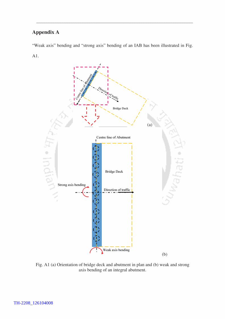
_____________________________________________________________________
Appendix A
“Weak axis” bending and “strong axis” bending of an IAB has been illustrated in Fig.
A1.
(a)
(b)
Fig. A1 (a) Orientation of bridge deck and abutment in plan and (b) weak and strong
axis bending of an integral abutment.
TH-2208_126104008

Appendix ______________________________________________________________________
152
Appendix B
Bridge Load Calculation
Bending Moment due to Dead Load (DL):
Density of Concrete = 25 kN/m3
Average Length of Span = 36.43 m
Depth of the Slab = 165 mm
Weight per m2 of slab = 0.165 × 25 = 4.125 kN/m2
Weight of wearing Course per m of slab = 2 kN
Total DL = 6.125 kN/m2
Total DL/span = 6.125 × 10 × 36.43 = 2231.4 kN
Shear Force at each support = 2231.4/2 = 1115.67 kN
Bending moment at the 1st interior support = 6.125 × 10 × 36.432/10 = 8128.76 kNm
Bending moment at other interior support moment = 6.125 × 10 × 36.432/12 = 6774 kNm
Deck Slab Design
Assuming, clear cover as 50 mm and diameter of the longitudinal bar as 10 mm.
Effective depth of slab = 165-(50+10) mm = 105 mm
Bending moment due to Live Load (LL): Class A wheeled vehicle with two-lane
loading
2 axle loads of 114 kN each are to be placed on span to carry maximum BM. At support the
Maximum LL = 114 kN (according to IRC: 6, 2010)
Width of dispersion parallel to span = 250 + 2 × (105+56) mm = 572 mm [Depth of wearing
course = 56 mm], which is less than the spacing of 1200 mm between the 114 kN axle loads.
So, the dispersion areas will not overlap.
Impact factor = 4.5/ (6+34.43) = 0.094
Effective width of slab perpendicular to span, bef = �. a. (1-a/ l0) +b1 = 10.18 m �10 m,
[From, Eq. B3.1, (IRC: 112, 2011)]
where, � = 1.052; a = 17.615 m; b1 = 0.612.
TH-2208_126104008

��������� ______________________________________________________________________
153
Intensity of loading/m width = 2 × 114 × 1.094 � 25 kN/m
SF at support due to LL = 25 × 10 × 0.572 × 2/2= 143 kN
Max BM at midspan (X-Z Plane) = 25 × 10 × (1.2+0.572)/2 – 143 = 78.5 kNm
1.5 load factor [IRC: 6 (2010), Table 3.4] and 20% of LL [IRC: 6 (2010), Cl. 219.5.2] will be
considered = 143 × 0.2 × 1.5= 42.9 kN
Total SF due to DL +LL = 1115.67+ 42.9 = 1158.5 kN
Vertical Load Calculation:
SF due to DL+LL = 1158.5 kN
DL from girders = 4 × 0.73 × 25 × 36.43 +10 × 1 × 0.73 × 25= 2841.89 kN
Design vertical load on each pier = 1158.5 + 2841.89 = 4001 kN
Assuming, factor of safety = 1.25
Designed axial load on pier = 5000 kN
TH-2208_126104008

Appendix ______________________________________________________________________
154
Appendix C
Pier Detailing according to IRC: 112-2011
Axial force on pier = 5000 kN
According to cl 16.2.2. (3), As, min = 0.10 × Ned/fyd = 1204.82 mm2
= 0.002 Ac = 5507 mm2
So, As, min = 5507 mm2
According to cl. 16.2.2. (4), Amax = 4% of Ac (without lap portion)
Assuming, As = 0.5% Ac = 13766 mm2
Providing, 24 Nos. 28 mm dia bar, longitudinal. As, pro = 14770 mm2
Transverse reinforcement (according to Cl. 16.2.3)
Cl. 16.2.3 (2), dia of horizontal ties = min of (8mm or 28/4 = 7 mm)
So, dia of transverse r/f = 8 mm
Cl. 16.2.3 (4), Spacing min of (i) 12 × 28 = 336 mm
(ii) Least dimension of column= 1700 mm
(iii) 200 mm
So, spacing = 200 mm
According to 17.2.1.1(3), confined r/f:
�k = 0.049<0.08 ; So, no need to provide confinement acc. to Cl 17.2.1.4
According to cl. 17.2.1.1(4), � �d = 0.024 mm2, where, �� = 1.16×10⁻³, Asw = 7 × area of
8mm dia. ties in a breadth of 1516mm.
So, minimum confined r/f should be provided according to Cl. 17.2.1.2
According to cl. 17.2.1.2 (2), �L = Ast, pro/Ac = 0.00536, �k = 0.049, � �, req = 0.022
� �d = max (0.022; 0.12) = 0.12
Spacing of the Ties:
According to cl. 17.2.1.3 (1), SL = min (5Db; 1/5th of the smallest dimension of concrete
core concrete) = min (140; 303.2) = 140mm
According to Cl. 17.2.1.3 (2), ST = min (1/3rd of the smallest dimension of concrete core
concrete; 200mm) = min (505.34 mm; 200 mm) = 200 mm
According to design potential hinges are not forming through the column. If it’s forming
then the buckling of longitudinal reinforcement will be taken care by Cl. 17.2.2.
Vertical and horizontal detailing of pier column (2000 mm × 1700 mm) are shown in
Figs. C.1 and C.2.
TH-2208_126104008
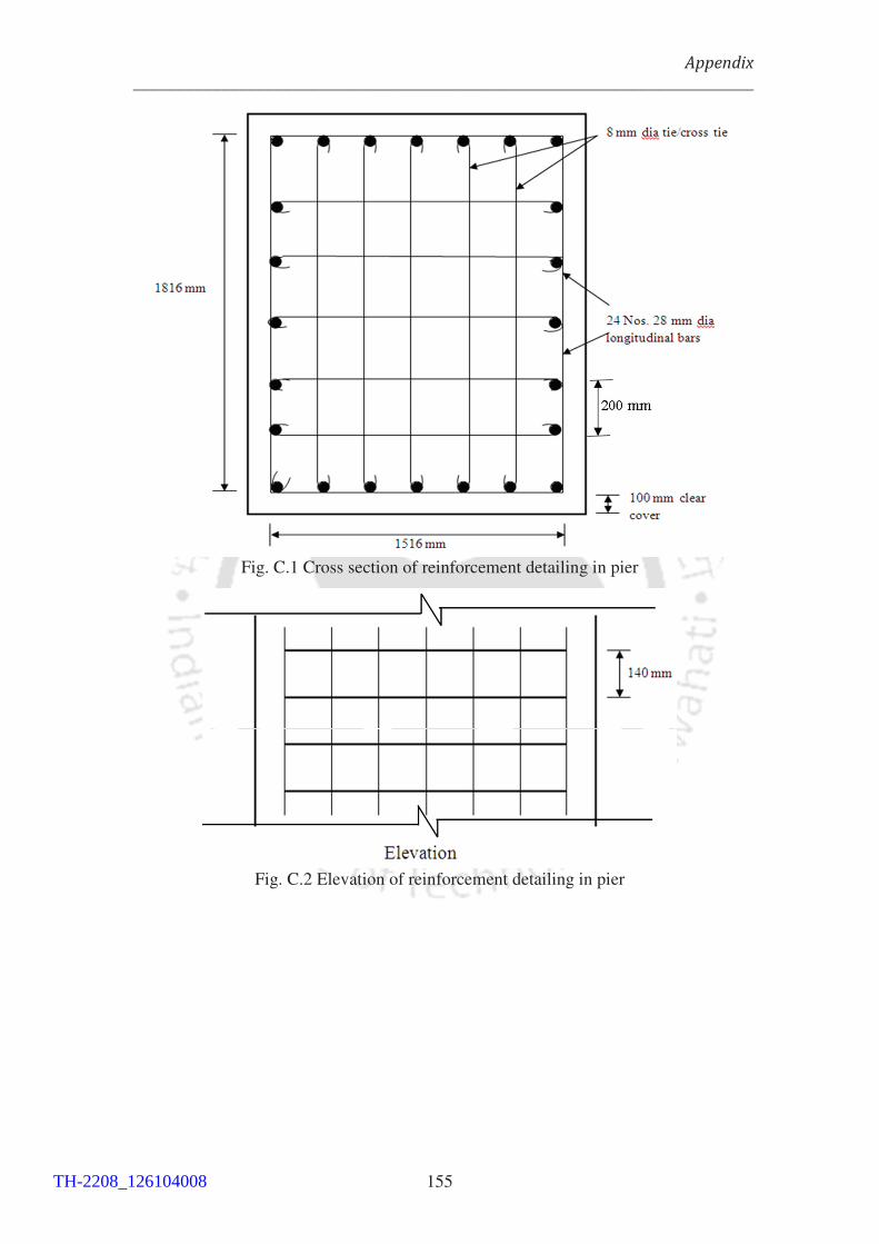
��������� ______________________________________________________________________
155
Fig. C.1 Cross section of reinforcement detailing in pier
Fig. C.2 Elevation of reinforcement detailing in pier
TH-2208_126104008

Appendix ______________________________________________________________________
156
Appendix D
Equivalent stiffness of pile group in OpenSees
From Ariyarathne et al. (2013), equivalent stiffness of pile group has been derived to
model the piles in OpenSees.
Equivalent stiffness of two pile in a row (Fig. D.1), Eeq × Aw = (Ep × Ap) + Es (Aw – Ap);
where,
Fig. D.1 Equivalent pile stiffness calculation
Aw = 5 × 1.372 = 6.86 m
Ep = 28E6 kN/m2
Ap = �
� × (1.372)2 m2= 2.955 m2
Es = 200440 kN/m2
Eeq . Aw = Ep × 2Ap + Es (Aw – 2Ap)
E eq = 12.188E6 kN/m2
Equivalent stiffness of one pile in a row:
Eeq . Aw = Ep . Ap + Es . (Aw – Ap)
Eeq = 6.20×10⁶ kN/m2
To consider the soil between the piles, the overall pile’s efficiency decreases by
considering p–multiplier.
For piles on soft clay, p–multipliers are as following according to Mokwa (1999):
Leading Row 0.80
1st trailing row 0.50
2nd trailing row 0.45
D DEq
Aw
TH-2208_126104008

��������� ______________________________________________________________________
157
During the cyclic loading, leading and 2nd trailing row pile efficiency get interchanged.
So, final stiffness of both the side rows E1 = E3 = 9.75×10⁶ kN/m2
Middle row equivalent stiffness E2= 3.1×10⁶ kN/m2
�
��� =
�
�� +
�
���+�
�
�; Eeq = 1.65×10⁶ kN/m2
As these three stiffnesses are in series in 2D plane, so equivalent pile group stiffness =
1.65×10⁶ kN/m2
TH-2208_126104008

Appendix ______________________________________________________________________
158
Appendix E
Pile length calculation in soft clay
Assume, length of pile l
Pier pile diameter, D = 1.372 m
Cross sectioned area of pile, Ap = 1.49 m2
Perimeter of pile, p = 4.31 m
Cohesion, c = 18 kN/m2
Nc = 9.0
The axial load carrying capacity of the pier piles is 500 kN.
Assuming, factor of safety (FOS) = 2.0, Ultimate load capacity (Qv)ult = Qp + Qf
(E.1)
End bearing capacity, Qp = Ap c Nc = 239.7 kN
Shaft friction, fs = c + �’h tan � = 18 kN/m2 [for, cohesive soil, � = 0]
Friction capacity, Qf = p fs �� �� � = 77.54l kN
So, equation D.1 becomes,
� 500×2 = 239.7 + 77.54l
� l = 10 m
So, length of the pier pile in soft clay is calculated as 10 m.
TH-2208_126104008

��������� ______________________________________________________________________
159
Appendix F
Calculations of API Curves in Medium Stiff Clay for Pier Pile
In medium stiff clay, soil cohesion c = 27 kN/m2
Unit density, � = 0.019 kN/m3
Pile diameter, D = 1372 mm
Perimeter of pile, p = 4.31E6 mm2
Strain at which half of maximum stress occurring, �c = 0.002
Actual lateral deflection = y
yc = 2.5 �c D = 6.86 mm
Where, �c = strain which occurs at one-half the maximum stress on laboratory undrained
compression tests of undisturbed soil samples.
XR = ��
�������� (F.1)
[Dimensionless empirical constant, J= 0.5]
∴XR is obtained as 5621 mm.
Ultimate resistance, pu (in kPa) = 3c + �� + ���
� (F.2)
Where, X= depth below soil surface
Applied force on a certain depth of pile, F = (Pu ×p) kN
Using all the parameters, lateral force-displacement curve for pier piles at the depths of 1
m and 4 m are shown in Table F.1.
Table F.1 Lateral force displacement curves for pier pile in medium stiff clay
1 m depth� 4 m depth�
Force (F), kN Displacement (y), m Force (F), kN� Displacement (y), m�
0 0 0 0
236.82 0.007 423.25 0.007
341.02 0.021 609.48 0.021
60.66 0.103 433.69 0.103
60.66408 � 433.6897 �
TH-2208_126104008

Appendix ______________________________________________________________________
160
Appendix G
Calculations of API curves in loose sand for pier pile
Pile diameter, D = 1372 mm,
Perimeter of pile, p = 4.31×106 mm2,
Coefficients are determined from Figure 6.8.6-1 of API (2000) as function of �´,
C1 = 1.6; C2 = 2.6; C3 = 23;
Effective unit weight of soil, � = 16 kN/m3,
Angle of internal friction of sand, � = 29°,
Initial modulus of subgrade reaction, k = 2170 kN/m3,
A factor to account for cyclic or static loading condition, A = 0.9 (for cyclic loading),
y = lateral deflection in m.
H = depth in m.
Ultimate lateral resistance at depth H, pu (in kN/m) = smallest of (pus, pud);
Where, pus = (C1 × H + C2 × D) × � × H (G.1)
and pud = C3 × D × H (G.2)
At the depth of 6 m from soil surface, the lateral force-displacement curves in loose sand
are derived below from API (2000) (section 6.8.6) for pier piles.
At 6 m depth, pus = 1264.051 kN and pud = 3029.376 kN
Then, the lateral soil resistance-deflection (p-y) relationship for sand at any specific depth
H, is approximated by the following expression:
P = A × pu × tanh ����
�� !� " (G.3)
The values of p-y curves at the depth 6 m in loose sand are shown in Table. G.1
TH-2208_126104008