JPL Publication 93-26, Vol. 2

Summaries of the Fourth Annual JPL Airborne Geoscience Workshop October 25-29, 1993 Volume 2. TlMS Workshop

Vincent J. Realmuto Editor

October 25, 1993

National Aeronautics and Space Adm~nistratlon

Jet Propulsion Laboratory Callfornla lnstltute of Technology Pasadena. Californ~a

This publication was prepared by the Jet Propulsion Laboratory, California Institute of Technology, under a contract with the National Aeronautics and Space Administration.

ABSTRACT

This publication contains the summaries for the Fourth Annual JPL Airborne Geoscience Workshop, held in Washington, D. C. on October 2529,1993. The main workshop is divided into three smaller workshops as follows:

The Airborne Visible/Infrared Imaging Spectrometer (AVIRIS) workshop, on October 2526. The summaries for this workshop appear in Volume 1.

The Thermal Infrared Multispectral Scanner (TIMS) workshop, on October 27. The summaries for this workshop appear in Volume 2.

The Airborne Synthetic Aperture Radar (AIRSAR) workshop, on October 28-29. The summaries for this workshop appear in Volume 3.

CONTENTS

Volume 1: AVIRIS Workshop

Use of Spectral Analogy to Evaluate Canopy Reflectance Sensitivity to Leaf Optical Property .................................................................................................... 1

Fre'dei-ic Buret, Vern C. Vanderbilt, Michael D. Steven, and Stephane Jacquemoud

A Tool for Manual Endmember Selection and Spectral Unmixing ....................... 3 C . Ann Bateson and Brian Curtiss

Lithologic Discrimination and Alteration Mapping From AVIRIS Data, Socorro, New Mexico .................................................................................................... 7

K . K. Beratan, N. DeLillo, A. Jacobson, R. Blom, and C. E. Chapin

Automating Spectral Unmixing of AVIRIS Data Using Convex Geometry ........................................................................................................................ Concepts .I 1

Joseph W. Boardman

AVIRIS Calibration Using the Cloud-Shadow Method ........................................... 15 K. L. Cardw, P. Reinersman, and R. F. Chen

Field Observations Using an AOTF Polarimetric Imaging Spectrometer ............. 19 Li-Jen Cheng, Mike Hamilton, Colin Mahoney, and George Reyes

Instantaneous Field of View and Spatial Sampling of the Airborne Visible/Infrared Imaging Spectrometer (AVIRIS) ................................................... 23

Thomas G. Chrien and Robert 0. Green

Airborne Visible/Infrared Imaging Spectrometer (AVIRIS): Recent Improvements to the Sensor ........................................................................................ 27

Thomas G. Chrien, Robert 0. Green, Charles M . Sarture, Christopher Chovit, Michael L. Eastwood, and Bjorn T . Eng

Comparison of Three Methods for Materials Identification and Mapping with Imaging Spectroscopy ......................................................................................... 31

Roger N. Clark, Gregg Swayze, Joe Boardman, and Fred Kruse

Comparison of Methods for Calibrating AVIRIS Data to Ground ................................................................................................................... Reflectance.. -35

Roger N . Clark, Gregg Swayze, Kathy Heidebrecht, Alexander F. H. Goetz, and Robert 0. Green

PW~QBPW PAGE i3ii,; ; Nb i i rini-c IV'

The U.S. Geological Survey, Digital Spectral Reflectance Library: Version 1: 0.2 to 3.0 pn ............................................................................................................... 37

Roger N . Clark, Gregg A. Swayze, Trude V . V . King, Andrea I . Gallagher, and Wendy M. Calvin

Application of a Two-Stream Radiative Transfer Model for Leaf Lignin and Cellulose Concentrations From Spectral Reflectance Measurements

............................................................................................................................. (Part 1) 39 Janres E . Conel, Jeannette van den Bosch, and Cindy I . Grove

Application of a Two-Stream Radiative Transfer Model for Leaf Lignin and Cellulose Concentrations From Spectral Reflectance Measurements

............................................................................................................................. (Part 2) 45 James E. Conel, Jeannette van den Bosch, and Cindy I . Grove

Discrimination of Poorly Exposed Lithologies in AVIRIS Data ............................. 53 William H. Farrand and Joseph C. Harsatzyi

................................................................... Spectral Decomposition of AVIRIS Data 57 Lisa Gaddis, Laurence Soderblom, Hugh Kieffer, Kris Becker, Jim Torson, and Kevin Miillins

Remote Sensing of Smoke, Clouds, and Fire Using AVIRIS Data ......................... 61 Bo-Cai Gao, Yoranr J . Kauf ian, and Robert 0. Green

Use of Data from the AVIRIS Onboard Calibrator ................................................... 65 Robert 0. Green

Inflight Calibration of AVIRIS in 1992 and 1993 ...................................................... 69 Robert 0. Green, Jarrles E . Cotzel, Mark Helmlinger, Jeannette zwn den Bosch, Chris Chozjit, and Tonz Chrien

Estimation of Aerosol Optical Depth and Additional Atmospheric Parameters for the Calculation of Apparent Reflectance from Radiance Measured by the Airborne Visible/Infrared Imaging Spectrometer ..................... 73

Robert 0. Green, Jarnes E. Conel, and Dnr A. Roberts

Use of the Airborne Visible/Infrared Imaging Spectrometer to Calibrate the Optical Sensor on board the Japanese Earth

...................................................................................................... Resources Sa tellite-1 77 Robert 0. Green, Jarnes E. Cotzel, Jeannette van den Bosch, and Masanobu Shimada

A Proposed Update to the Solar Irradiance Spectrum Used in LOWTRAN and MODTRAN ............................................................................................................ 81

Robert 0. Green and Bo-Cai Gao

A Role for AVIRIS in the Landsat and Advanced Land Remote Sensing System Program ............................................................................................................ -85

Robert 0. Green and John J. Sinztnonds

Estimating Dry Grass Residues Using Landscape Integration Analysis .............. 89 Quinn J . Hart, Susan L. Ustin, Lian Duan, and George Scheer

Classification of High Dimensional Multispectral Image Data .............................. 93 Joseph P. Hoffbeck and David A. Landgrebe

Simulation of Landsa t Thema tic Mapper Imagery Using AVIRIS Hyperspectral Imagery ................................................................................................. 97

Linda S. Kalman and Gerard R. Peltzer

The Effects of AVIRIS Atmospheric Calibration Methodology on Identification and Quantitative Mapping of Surface Mineralogy, Drum Mtns., Utah ......................................................................................................... 101

Fred A. Kruse and John L. Dwyer

AVIRIS Spectra Correlated With the Chlorophyll Concentration of a Forest Canopy ............................................................................................................................ 105

John Kupiec, Geoffyey M. Smith, and Paul J. Curran

AVIRIS and TIMS Data Processing and Distribution at the Land Processes Distributed Active Archive Center ............................................................................. 109

G. R. Mah and J. Myers

Measurements of Canopy Chemistry With 1992 AVIRIS Data at ...................................................................... Blackhawk Island and Harvard Forest 113

Mary E. Martin and John D. Abev

Classification of the LCVF AVIRIS Test Site With a Kohonen ............................................................................................ Artificial Neural Network 117

Erzse'bet Mereizyi, Robert B. Singer, and William H. Farrand

Extraction of Auxiliary Data from AVIRIS Distribution Tape for Spectral, Radiometric, and Geometric Quality Assessment ................................................... 121

Peter Meyer, Robert 0. Green, and Thomas G. Chrien

Preprocessing: Geocoding of AVIRIS Data using Navigation, Engineering, DEM, and Radar Tracking System Data .................................................................... 127

Peter Meyer, Steven A. Larson, Ear2 G. Hansen, and Klaus I. Ztten

The Data Facility of the Airborne Visible/Infrared Imaging Spectrometer ......................................................................................................................... (AVIRIS) .I33

Pia J. Nielsen, Robert 0. Green, Alex T. Murray, Bjorn T . Eng, H. Ian Novack, Manuel Solis, and Martin Olah

Mapping of the Ronda Peridotite Massif (Spain) From AVIRIS Spectro- Imaging Survey: A First Attempt ............................................................................... 137

P. C. Pinet, S. Chabrillat, and G. Ceuleneer

Spectral Variations in a Collection of AVIRIS Imagery ........................................... 141 John C. Price

Monitoring Land Use and Degradation Using Satellite and .............................................................................................................. Airborne Data ..I45

Terrill W. Ray, Thomas G. Farr, Ronald G. Blom, and Robert E . Crippen

The Red Edge in Arid Region Vegetation: 340-1060 nm Spectra ........................... 149 Terrill W. Ray, Bruce C. Murray, A. Chehbouni, and Eni Njoku

Temporal Changes in Endmember Abundances, Liquid Water and Water Vapor Over Vegetation at Jasper Ridge ..................................................................... 153

Dar A. Roberts, Robert 0. Green, Donald E . Sabol, and John B. Adams

Mapping and Monitoring Changes in Vegetation Communities of Jasper .................... Ridge, CA, Using Spectral Fractions Derived From AVIRIS Images 157

Donald E. Sabol, Jr., Dar A. Roberts, John B. Adams, and Milton 0. Smith

The Effect of Signal Noise on the Remote Sensing of Foliar Biochemical ................................................................................................................ Concentration 161

Geoffrey M . Smith and Paul J. Currarl

Application of MAC-Europe AVIRIS Data to the Analysis of Various Alteration Stages in the Landdmannalaugar Hydrothermal Area (South

............................................................................................................................ Iceland) 165 S. Sommer, G. Lorcher, and S. Endres

Estimation of Crown Closure From AVIRIS Data Using Regression .......................................................................................................................... Analysis 169

K . Staenz, D. J. Williams, M . Truchon, and R. Fritz

Optimal Band Selection for Dimensionality Reduction of ................................................................................................. Hyperspectral Imagery 173

Stephen D. Stearns, Bruce E . Wilson, and James X. Peterson

viii

Objective Determination of Image End-Members in Spectral Mixture Analysis of AVIRIS Data ............................................................................... 177

Stefanie Tompkins, John F. Mustard, Carle M . Pieters, and Donald W . Forsyth

Relationships Between Pigment Composition Variation and Reflectance ........................................ for Plant Species from a Coastal Savannah in California 181

Susan L. Ustin, Eric W . Sanderson, Yaffa Grossman, Quinn J. Hart, and Robert S . Haxo

Atmospheric Correction of AVIRIS Data of Monterey Bay Contaminated by Thin Cirrus Clouds .................................................................................................. 185

Jeannette van den Bosch, Curtiss 0. Davis, Curtis D. Mobley, and W . Joseph Rhea

Investigations on the 1.7 p Residual Absorption Feature in the ............................................................................... Vegetation Reflection Spectrum.. -189

J. Verdebout, S . Jacquernoud, G. Andreoli, B. Hosgood, and A. Sieber

A Comparison of Spectral Mixture Analysis and NDVI for Ascertaining ..................................................................................................... Ecological Variables -193

Carol A. Wessman, C. Ann Bateson, Brian Curtiss, and Tracy L. Benning

Using AVIRIS for In-Flight Calibration of the Spectral Shifts of Spot-HRV ............................................................................................................. and of AVHRR? 197

Veronique Willart-Souflet and Richard Santer

Laboratory Spectra of Field Samples as a Check on Two Atmospheric .................................................................................................... Correction Methods ..201

Pung Xu and Ronald Greeley

Determination of Semi-Arid Landscape Endmembers and Seasonal Trends Using Convex Geometry Spectral Unmixing Techniques ....................................... 205

Roberta H. Yuhas, Joseph W . Boardman, and Alexander F. H. Goetz

Slide Captions ................................................................................................................ 209

Volume 2: TIMS Workshop

..................................... Estimation of Spectral Emissivity in the Thermal Infrared 1 David K yskowski and J. R. Maxwell

The Difference Between Laboratory and in-situ Pixel-Averaged Emissivity: The Effects on Temperature-Emissivity Separation ................................................. 5

Tsuneo Matsunaga

Mineralogic Variability of the Kelso Dunes, Mojave Desert, California Derived From Thermal Infrared Multispectral Scanner (TIMS) Data ................... 9

Michael S. Ramsey, Douglas A. Howard, Philip R. Christensen, and Nicholas Lancaster

Remote Identification of a Gravel Laden Pleistocene River Bed ............................ 13 Douglas E. Scholen

Volume 3: AIRSAR Workshop

Interferometric Synthetic Aperture Radar Imagery of the .................................................................................................................... Gulf Stream 1

T. L. Ainsworth, M . E . Cannella, R. W. Jansen, S. R. Chubb, R. E . Carande, E . W. Foley, R. M . Goldstein, and G. R. Valenzuela

MAC-91: Polarimetric SAR Results on Montespertoli Site ..................................... 5 S . Baronti, S . Luciani, S. Moretti, S. Paloscia, G. Schiavon, and S . Sigismondi

AIRSAR Views of Aeolian Terrain ............................................................................. 9 Dan G. Blumberg and Ronald Greeley

Glaciological Studies in the Central Andes Using AIRSAR/TOPSAR ................. 13 Richard R. Forster, Andrew G. Klein, Troy A. Blodgett, alrd Bryan L. lsacks

Estimation of Biophysical Properties of Upland Sitka Spruce (Picea Sitchensis) Plantations ....................................................................................... 17

Robert M . Green

Forest Investigations by Polarimetric AIRSAR Data in the Harz Mountains ....................................................................................................................... 21

M . Keil, D. Poll, J . Raupenstmuch, T . Tares, and R. Winter

Comparison of Inversion Models Using AIRSAR Data for ............................................................................................... Death Valley, California 25

Kathryn S. Kierein-Young

Geologic Mapping Using Integrated AIRSAR, AVIRIS, and TIMS Data ....................................................................................................................... 29

Fred A. Kruse

Statistics of Multi-look AIRSAR Imagery: A Comparison of Theory With ............................................................................................................... Measurements .33

J. S . Lee, K . W. Hoppel, and S . A. Mango

AIRSAR Deployment in Australia, September 1993: Management and Objectives ....................................................................................... 37

A. K. Milne and I . J. Tapley

Current and Future Use of TOPSAR Digital Topographic Data for Volcanological Research ............................................................................................... 41

Peter J. Mouginis-Mark, Scott K. Rowland, and Harold Garbeil

Preliminary Analysis of the Sensitivity of AIRSAR Images to . . Soil Moisture Vans t~ons ............................................................................................... 45

Rajan Pardipuram, William L. Teng, James R. Wang, and Edwin T . Engman

Unusual Radar Echoes From the Greenland Ice Sheet ............................................ 49 E. J. Rignot, J. J. van Zyl, S . J . Ostro, and K. C. Jezek

MAC Europe '91 Campaign: AIRSAR/AVIRIS Data Integration for ........................................................................... Agricultural Test Site Classification 53

S . Sangiovanni, M . F. Buongiorno, M . Ferrarini, and A. Fiumara

Measurement of Ocean Wave Spectra Using Polarimetric AIRSAR Data ................................................................................................................ .57

D. L. Schuler

An Improved Algorithm for Retrieval of Snow Wetness Using C-Band AIRSAR ............................................................................................................ 61

Jiancheng Shi, Jeff Dozier, and Helmut Rott

Polarimetric Radar Data Decomposition and Interpretation ................................ -65 Guoqing Sun and K. Jon Ranson

Synergy Between Optical and Microwave Remote Sensing to Derive Soil and Vegetation Parameters From MAC Europe 91 Experiment ....... 69

0. Taconet, M . Benallegue, A. Vidal, D. Vidal-Madjar, L. Prevot, and M. Normand

SAR Terrain Classifier and Mapper of Biophysical Attributes .............................. 73 Fawwaz T . Ulaby, M . Craig Dobson, Leland Pierce, and Kamal Sarabandi

Classification and Soil Moisture Determination of Agricultural Fields ................ 77 A. C. van den Broek and J. S . Groot

Relating P-Band AIRSAR Backscatter to Forest Stand Parameters ........................ 81 Yong Wang, John M . Melack, Frank W, Davis, Eric S . Kasischke, and Norman L. Christensen, Jr.

Soil Moisture Retrieval in the Oberpfaffenhofen Testsite Using MAC Europe AIRSAR Data ................................................................................................... 85

Tobias Wever and lochen Henkel

Microwave Dielectric Properties of Boreal Forest Trees ......................................... 89 G . Xu. F . Ahern. and J . Brown

Slide Captions ................................................................................................................ 93

xii

Estimatbn of spedral emissivily h the thennal Infrared

David Kryskowski and J. R. Maxwell

Environmental Research Institute of Michigan 3300 Plymouth Rd., Ann Arbor, Michigan 48105

1. INTRODUCTION

A number of algorithms are available in the literature that attempt to remove most of the effects of temperature from thermal multispectral data where the final goal is to extract emissivity differences. Early approaches include adjacent spectral band ratioing, broad band radiance normalization and the use of one band where emissivities are generally high (e.g., 11 to 12 pm) to determine the temperature (Salisbury, 1992). More recent work (Salisbury, 1992) has produced two techniques that use data averaging to extract temperature to leave a quantity related to emissivity changes. These two techniques (Thermal Log Residuals and Alpha Residuals) have been investigated and compared and appear to provide reasonable results.

The analysis presented in this paper develops a thermal IR multispectral temperature/emissivity estimation procedure based on formal estimation theory, Gaussian statistics, and a stochastic radiance signal model including the effects of both temperature and emissivity. The importance of this work is that this is an optimal estimation procedure which will provide minimum variance estimates of temperature and emissivity changes directly.

Section 2 discusses optimal linear spectral emissivity estimation and Section 3 is a summary.

2. OPTIMAL LINEAR SPECTRAL EMlSSlVlTY ESTIMATION

A stochastic model for the spectral radiance in the thermal IR using the Planck equation ignoring reflection and atmospheric contributions is:

CI First Radiation Constant c2 - Second Radiation Constant T Average background temperature in region ? ( A ) Average background emissivity in region A Wavelength AT Change in background temperature (a zero mean random variable) A e ( l ) Change in background emissivity (a zero mean random process)

The term in braces in Equation 1 is the apparent emissivity, ~ ~ ~ ( h ) . The model assumes samples are independent and identically distributed spatially. From Equation 1 it is clear that changes in temperature affect all wavelengths uniformly. Thus AT can be considered as a random process of rank

one with respect to wavelength. In a generalized sense it is also considered to be narrowband since all of the variation induced by temperature will fall along a single direction with a properly chosen expansion basis for the spectral radiance. The covariance of the apparent emissivity can be computed assuming that temperature and emissivity are independent as :

The second term on the right hand side of Equation 2 is (to within the temperature variance) known. Moreover in an absolute sense the second term more often is the dominant one (thermal IR phenomenology tells us this, especially in the daytime) since it is the one dependent on temperature. The first term on the right hand side of the equation is more difficult to specify. In order to describe it for a certain class of material an ensemble of measurements is needed for that class. Since only a very limited number of measurements exist for spectral emissivity in the thermal IR, a description of the first term for an arbitrary class is not available. In this development it will be assumed that the first term is stationary white. That is:

This assumption is very appealing for large regions because &rge regions usually contain many different classes of materials and it is reasonable to assume the second order statistics of the ensemble are white.

2.1 Cancellation of Namw Band Interference (Temperature)

What follows here is a procedure for separating temperature and emissivity. What motivates the procedure is the observation that emissivity and temperature cannot be separated from a single multispectral measurement but a statistically based procedure can provide separation with acceptable error. Again writing Equation 1 but including sensor noise w(A):

Since the means are assumed to be known or well estimated from the data, the mean radiance can be subtracted off along with a division by the blackbody function to obtain the following equation for observed variation in apparent emissivity:

The quantity &(A) contains the relative ernissivity behavior and it is this component that needs to be estimated. To estimate a realization of the random process A&@), the covariance of the apparent

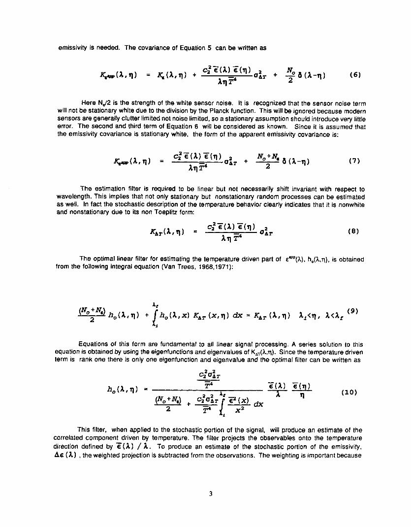
emissivity is needed. The covariance of Equation 5 can be written as

Here NJ2 is the strength of the white sensor noise. It is recognized that the sensor noise term will not be stationary white due to the division by the Planck function. This will be ignored because modern sensors are generally clutter limited not noise limited, so a stationary assumption should introduce very little error. The second and third term of Equation 6 will be considered as known. Since it is assumed that the emissivity covariance is stationary white, the form of the apparent emissivity covariance is:

The estimation filter is required to be linear but not necessarily shift invariant with respect to wavelength. This implies that not only stationary but nonstationary random processes can be estimated as well. In fact the stochastic description of the temperature behavior clearly indicates that it is nonwhite and nonstationary due to its non Toeplitz form:

The optimal linear filter for estimating the temperature driven part of eVP(3C), h,(h,q), is obtained from the following integral equation (Van Trees, 1968,1971):

Equations of this form are fundamental to all linear signal processing. A series solution to this equation is obtained by using the eigenfunctions and eigenvalues of K,(h,q). Since the temperature driven term is rank one there is only one eigenfunction and eigenvalue and the optimal filter can be written as

This filter, when applied to the stochastic portion of the signal, will produce an estimate of the correlated component driven by temperature. The filter projects the observables onto the temperature direction defined by =(a) / A . To produce an estimate of the stochastic portion of the emissivity, Aa ( A ) , the weighted projection is subtracted from the observations. The weighting is important because

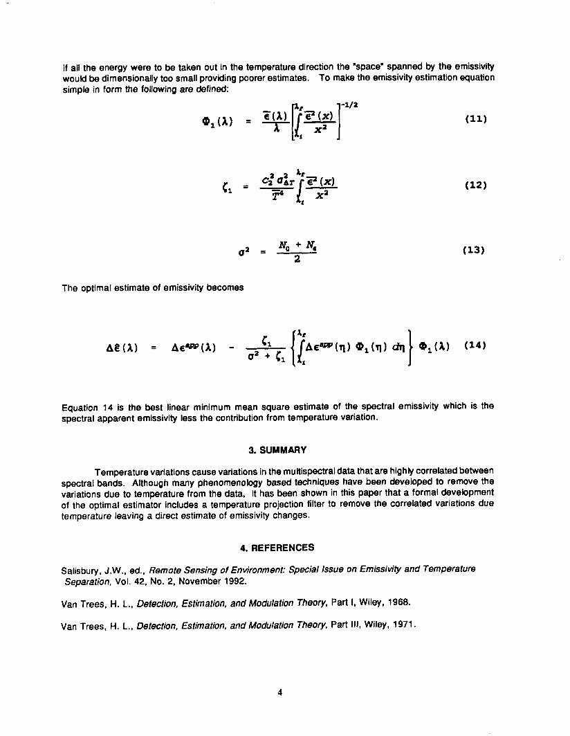
if all the energy were to be taken out in the temperature direction the "space" spanned by the emissivity would be dimensionally too small providing poorer estimates. To make the emissivity estimation equation simple in form the following are defined:

The optimal estimate of emissivity becomes

Equation 14 is the best linear minimum mean square estimate of the spectral emissivity which is the spectral apparent emissivity less the contribution from temperature variation.

3. SUMMARY

Temperature variations cause variations in the multispectral data that are highly correlated between spectral bands. Although many phenomenology based techniques have been developed to remove the variations due to temperature from the data, it has been shown in this paper that a formal development of the optimal estimator includes a temperature projection filter to remove the correlated variations due temperature leaving a direct estimate of emissivity changes.

4. REFERENCES

Salisbury , J. W., ed., Remote Sensing of Environment: Special Issue on Ernissivity and Temperature Separation, Vol. 42, No. 2, November 1992.

Van Trees, H. L., Detection, Estimation, and Modulation Theory, Part I , Wiley, 1968.

Van Trees, H. L., Detection, Estimation, and Modulation Theory, Part Ill, Wiley, 1971 .

THE DIFFERENCE BETWEEN LABORATORY AND IN-SITU PIXEL-AVERAGED EMISSIVITY:

THE EFFECTS ON TEMPERATURE-EMISSIVITY SEPARATION

Tsuneo Matsunaga

Geophysics Department, Geological Survey of Japan 1-1-3, Higashi, Tsukuba, Ibaraki, 305, Japan

1. INTRODUCTION

Advanced Spaceborne Thermal Emission and Reflection Radiometer(ASTER) is a Japanese future imaging sensor which has five channels in thermal infrared(T1R) region. To extract spectral emissivity information from ASTER and/or TIMS data, various temperature-emissivity(T-E) separation methods have been developed to date. Most of them require assumptions on surface emissivity, in which emissivity measured in a laboratory is often used instead of in-situ pixel-averaged emissivity. But if these two emissivities are different, accuracies of separated emissivity and surface temperature are reduced.

In this study, the difference between laboratory and in-situ pixel-averaged emissivity and its effect on T-E separation are discussed. TIMS data of an area containing both rocks and vegetation were also processed to retrieve emissivity spectra using two T- E separation methods.

2. THE DIFFERENCE BETWEEN LABORATORY AND IN-SITU PIXEL-AVERAGED EMISSIVITY OF LAND SURFACE

The difference between laboratory and in-situ pixel-averaged emissivity has several causes. A pixel generally contains different materials of different temperatures. Since a pure isothermal sample is usually measured in a laboratory, laboratory emissivity may differ from pixel-averaged emissivity(heterogeneity effect).

Due to less-than-unity emissivity of land surface, incident thermal radiation to the surface is partially reflected and observed by a sensor. Incident radiation consists of downwelling radiance from the atmosphere including clouds and thermal radiation from the surrounding. In addition to reflection, the surface roughness causes scattering of thermal emission from the surface itself. Thus, apparent emissivity is expected to be higher than laboratory emissivity because of these scatteringlreflection effect.

3. TEMPERATURE-EMISSIVITY SEPARATION METHODS

In this study, Emissivity Spectrum Normalization(ESN: Realmuto, 1990) and Mean-Maximum Difference(MMD: Matsunaga, 1993a, b) methods were considered. The MMD method is based on a relationship between the mean and the spectral variation of emissivity of terrestrial materials in TIR region. Similar methods have been developed by Kealy and Gabell [1990], Stoll [I9911 and Hook [personal communication]. In the MMD method, the relationship between the mean(M) and the difference between the maximum and the minimum(Maximum Difference: MD) of emissivity for TIMS six channels is assumed to be linear. MD corresponds to spectral contrast or variation. Surface tempera- ture and spectral emissivity can be separated based on this assumption. Fig. 1 shows M- MD relationship for various earth's surface materials. Volcanic rocks have high contrast and low mean of spectral emissivity. On the contrary, spectra of water surface and vegetation are very flat and close to unity. This relationship can be approximated to linear, though the distribution is somewhat scattered.

4. EVALUATION OF EFFECTS OF SURFACE HETEROGENEITY AND SCATTERINGIREFLECTION BY SIMPLE SIMULATIONS

4.1. Surface Heterogeneity

Pixel-averaged emissivity of an isothermal pixel comprised of two materials

Fig. 1

Felsic Rocks Intermediate Rocks Mafic-Ultra Mafic Rocks Sedimentary Rocks Metamorphic Rocks Soil Vegetation Wateralce Coatings

Maximum Difference

Mean-maximum difference relationship for various terrestrial materials.

0.70 Ch. t Ch. 2 Ch. 3 Ch. 4 Ch. 5 Ch. 6

TIMS Channel 0 0.05 0.1 0.15 0.2

Maximum Difference

Fig. 2 Pixel-averaged emissivity spectra(a) and M-MD relationship(b) for varying areal fraction of conifer foliage.

having different spectral emissivity was calculated to evaluate the heterogeneity effect on spectral emissivity. Rhyolite and conifer foliage were chosen as the materials because volcanic rocks and vegetation generally have very different emissivity spectra. Simulated pixel-averaged emissivity spectra corresponding to varying conifer foliage area fraction are shown in Fig. 2a. Maximum emissivity increases according to the fraction. Therefore, assuming constant maximum emissivity in the ESN method causes errors if vegetation fraction in a pixel varies within a scene. Fig. 2b shows M-MD relationship for this case. Specua of mixed pixels almost satisfy the linear relationship determined from pure rhyolite and conifer foliage spectra.

4.2. Surface ScatteringfReflection of Thermal Radiation

Because detailed calculation of scattering/reflection effects at land surface is difficult, single reflection effect was considered in case of the geometry shown in Fi The surface was illuminated by thermal emission from the surrounding wall. Both o f. 3. them were assumed to be isothermal and isotropic reflectors/emitters with same emissiv- ity as rhyolite and have same temperature. Long-wave sky radiation was ignored. Simu- lated emissivity spectra were shown in Fig. 4a for varying angle 8. As 8 decreases, spectral contrast decreases and emissivity values increases. Thus, neglecting the scatter- ing/reflection effect on surface emissivity results in overestimation of surface tempera- ture. M-MD relationship was linear for varying €)(Fig. 4b).

These simulations show that the effects of surface heterogeneity and scattering/ reflection can change in-situ pixel-averaged emissivity from the value measured in a laboratory. The robustness of the assumption used in the MMD method is also shown.

5. EXTRACTION OF EMISSIVITY SPECTRA FROM TIMS DATA

5.1. Acquisition and Atmospheric Correction of TIMS Data

Radiometer / \

Wall (EW, T w ) Fig. 3 A simple model for the simulation

~ u r f a c e (ES, Ts) of scattering/reflection effect at the surface. ? / / / / / / / / / / / / / /

1.00 a) J -

i % i 2 0.95 -.....-... 4 .... b .... ........... ........... ;.-

4 90" .- > i \ i \ ; ' I 1 .- 0.90 YI--* ............ i ...... \.; ............,. 1

p- 30" W . 10" \ i '

0.85 1 ......... .......... 4 &..\...;.< 1 B I

" " ~ " " ~ " " ~ " " 1 ' -

1 2 3 4 5 6 0 0.05 0.1 0.15 0.2 TlMS Ch. Maximum Difference

Fig. 4 Apparent emissivity spectra(a) and M-MD relationship(b) including single reflection effect. The surface and the wall were assumed to have rhyolite emissivity spectrum and same temperature.

TIMS data used in this study were acquired over Mono Lake/Mammoth Lakes area, California, on October 16, 1991. This area is located at the east flank of the Sierra Nevada. Flight altitude, spatial and temperature resolutions were about 7.5 km ASL, 13 m, and 0.25 - 0.30°C, respectively.

Atmospheric transmittance and upwelling radiance for each TIMS channel were preliminarily calculated using LOWTRAN7 with data from a radiosonde launched at the time of the overflight. Though lake surface brightness temperatures for TIMS Ch. 5 and 6 were same after LOWTRAN-based atmospheric correction, temperature for Ch. 1,2, and 4 were higher than Ch. 5 and 6(Fig. 5) This discrepancy was also found at dark-grayish sand beach with a little grass. In this study, atmospheric transmittance and upwelling radiance calculated from TIMS data of the lake surface and the beach were used. For this calculation, it was assumed that these two sites were blackbody and brightness tempera- tures in Ch. 5 after LOWTRAN-based aunospheric correction were true surface tempera- tures.

5.2. Temperature-Emissivity Separation

The ESN and the MMD methods were applied to atmospherically corrected TIMS radiance data to retrieve surface emissivity spectra. Fig. 6 shows retrieved spectra for the transect from a coniferous forest to rhyolite-dominated field at the flank of Crater Mountain. Both methods could obtain emissivity troughs corresponding to Si02 content for rhyolite, and flat spectra for forest. In addition, the MMD method could show higher emissivity values for the forest than for rhyolite and transitional spectra from forest to rhyolite(Point 57 and 58).

6. CONCLUSION

Simple simulations showed that in-situ pixel-averaged emissivity may differ from emissivity measured in a laboratory due to the effects of surface heterogeneity and scatteringlreflection. It was also shown that T-E separation methods based on the rela- tionship between the mean and the variation of spectral ernissivity are relatively robust to these effects. It must be noted, however, that retrieved emissivity by these methods is apparent and still including scattering/reflection contribution.

ACKNOWLEDGEMENTS

The author would like to thank Dr. S. Rokugawa and Mr. H. Tonooka, Univer-

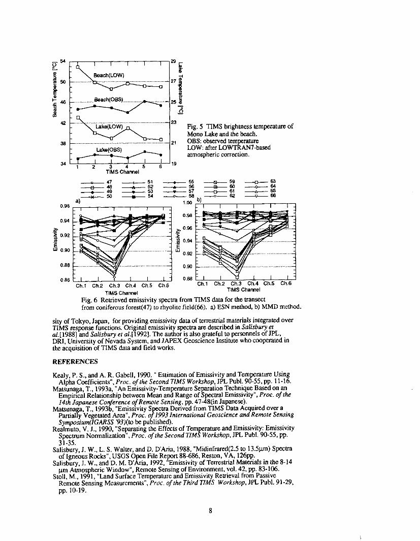
Fig. 5 TIMS brightness temperature of Mono Lake and the beach.

..................................................................... 21 OBS: observed temperahue Lake(0BS) LOW: after LOWTRAN7-based

a atmospheric correction. - 1; 3 l9

TIMS Channel - 47 .-~ 51 n 48 ---b-- 52 - 49 --e-- 53 - 5 0 .-54

..........................

Ch.1 Ch.2 Ch.3 Ch.4 Ch.5 Ch.6 TIMS Channel TIMS Channel

Fig. 6 Retrieved emissivity spectra from TIMS data for the uansect from coniferous forest(47) to rhyolite field(66). a) ESN method, b) MMD method.

sity of Tokyo, Japan, for providing emissivity data of terrestrial materials integrated over TIMS response functions. Original emissivity spectra are described in Salisbury et a1.[1988] and Salisbury et a1.[1992]. The author is also grateful to personnels of JPL, DRI, University of Nevada System, and JAPEX Geoscience Institute who cooperated in the acquisition of TIMS data and field works.

REFERENCES

Kealy, P. S., and A. R. Gabell, 1990. " Estimation of Emissivity and Temperature Using Alpha Coefficients", Proc. of the Second TIMS Workshop, JPL Publ. 90-55, pp. 11-16.

Matsunaga, T., 1993a. "An Emissivity-Temperature Separation Technique Based on an Empirical Relationship between Mean and Range of Spectral Emissjvity", Proc. of the 14th Japanese Cor$erence of Remote Sensing, pp. 47-48(in Japanese).

Matsunaga, T., 1993b. "Emissivity Spectra Derived from TIMS Data Acquired over a Partially Vegetated Area", Proc. of 1993 International Geoscience and Remote Sensing Symposium(1GARSS '93)(to be published).

Realmuto, V. J., 1990, "Separating the Effects of Temperature and Emissivity: Emissivity Spectrum Normalization", Proc. of the Second TlMS Workshop, JPL Publ. 90-55, pp. 71-15. - - --.

Salisbury, J. W., L. S. Walter, and D. D'Aria, 1988, "Midinfrared(2.5 to 13.5pm) Spectra of Igneous Rocks", USGS Open File Report 88-686, Reston, VA, 126pp.

Salisbury, J. W., and D. M. D'Aria, 1992, "Emissivity of Terrestrial Materials in the 8-14 pm Atmospheric Window", Remote Sensing of Environment, vol. 42, pp. 83-106.

Stoll, M., 1991, "Land Surface Temperature and Emissivity Retrieval from Passive Remote Sensing Measurements", Proc. of [he Third TlMS Workshop, JPL Publ. 91-29, pp. 10-19.

MINERALOCIC VARIABILITY OF THE KELSO DUNES, MOJAVE DESERT, CALIFORNIA DERIVED FROM THERMAL INFRARED

MULTISPECTRAL SCANNER (TIMS) DATA

Michael S. ~ a m s e ~ l , Douglas A. ~owardl , Philip R. christensenl and Nicholas Lancaster2

l~e~ar t rnent of Geology 2Desert Research Institute Arizona State University 7010 Dandini Blvd.

Tempe, Arizona 85287- 1404 Reno, Nevada 895 12

Mineral identification and mapping of alluvial material using thermal infrared (TIR) remote sensing is extremely useful for tracking sediment transport, assessing the degree of weathering and locating sediment sources. As a result of the linear relation between a mineral's percentage in a given area (image pixel) and the depth of its diagnostic spectral features, TIR spectra can be deconvolved in order to ascertain mineralogic percentages (Ramsey and Christensen, 1992; Gillespie, et al., 1990). Typical complications such as vegetation, particle size and thermal shadowing (Ramsey and Christensen, 1993) are minimized upon examination of dunes. Actively saltating dunes contain little to no vegetation, are very well sorted and lack the thermal shadows that arise from rocky terrain. The primary focus of this work was to use the Kelso Dunes as a test location for an accuracy analysis of temperature/emissivity separation and linear unmixing algorithms. Accurate determination of ground temperature and component discrimination will become key products of future ASTER data.

A decorrelation stretch of the TIMS image showed clear color variations within the active dunes. Samples collected from these color units were analyzed for mineralogy, grain size, and separated into endmembers. This analysis not only reveled that the dunes contained significant mineralogic variation (Fig. I), but were more immature (low quartz percentage) then previously reported (Sharp, 1966; Yeend, eta]., 1954). Unmixing of the TIMS data using the primary mineral endmembers produced uniquc variations within the dunes and may indicate near, rather than far, source locales for the dunes.

The Kelso Dunes lie in the eastern Mojave Desert, California approximately 95 km west of the Colorado River. The primary dune field is contained within a topographic basin bounded by the Providence, Granite, Bristol and Kelso Mountains to the east, south, west and north, respectively. The dune field rests upon the alluvial fans which extend from the Providence and Granite Mountains, with the active region marked by three northeast trending linear ridges. Although active, the dunes appear to lie at an opposing regional wind boundary which produces little net movement of the crests (Sharp, 1966). Previous studies have estimated the dunes range from 70% (Sharp, 1966) to 90% (Paisley, et al., 1991) quartz mainly derived from a source 40 km to the west. The dune field is assumed to have formed in a much more arid climate than present, with the age of the deposit estimated at greater than 100,000 years (Yeend, et al., 1984).

Klc KZI K3c K4r KSc K61 K13c K17c W K P c KUc K40c K42c

Figure 1. Mineral percentages derived fiom point-counts of thirteen sand samples. Sample numbers represent the collection site with a 'c' or 'st extension indicating a dune crest or swale. Samples Klc through K6s were collected from the same color unit and analyzed to verify the accuracy of the point-counting technique (note the similarity of the percentages). Samples K13c through K42c were collected along a 9.5 km N-S traverse through the most active region of the dune field (note the variation when compared to the first six samples). Also significant is the low average quartz percentage (40.4%).

2. SAMPLE ANALYSES

Forty-eight bulk samples were collected along a 9.5 km N-S traverse. These samples represented different image color units as well as position on the dune (crest vs. swale). Thirteen of the forty-eight bulk samples were chosen for detailed analyses to determine modal abundances. Six of these were fiom a small, mineralogically similar

Magnetile M

1400 1200 1000 800 600 400 Wavenumber

Figure 2. Laboratory emission spectra of the four endmembers - quartz, plagioclase, K-feldspar and magnetite (Avg. grain diameter = 500 - 710 p). Minerals were separated from bulk samples using magnetic and heavy liquid separation techniques.

rcgion and acted as a check on the consistency of the laboratory analysis. The bulk sand was split into 20 g samples (Cadle, 1955) from which thin sections and laboratory emission spectra were obtained (Christensen and Harrison, 1992). Over 200 grains per sample were counted to determine mineralogy and particle diameters (Jones, 1987). Samples K13c - K42c show clear mineralogic variations throughout the dune field (Fig. 1). These variations appear real based upon: (I) the color variations in the TIMS image; (2) the differences in the laboratory emission spectra; and (3) the similar point count results from samples Klc - K6s. Certain samples, collected from low-lying areas, contained appreciable amounts of clay. The clay component, separated from the sand using a Na-pyrophosphate dispersent, was analyzed by X-ray diffraction and found to be primarily montmorillonite. Finally, approximately 4 g of the dominant mineralogic components were separated using heavy liquid (Na polytungstate) and magnetic separation. While tedious, this separation insured the use of the correct endmembers for the dunes. Because the spectrum of plagioclase, for example, can vary dramatically as a function of An number, separation is preferred over the use of library spectra. The spectra of these endmember minerals (Fig. 2) were used as inputs into the unmixing algorithm for both the lab and image spectra.

70 [3 % Magnetite

Figure 3. Comparison of endmember percentages derived from point counts (fist bar) and the unmixing model (second bar). The three samples show the best, average and worst case error.

Thermal Infrared Multispectral Scanner (TIMS) data for the Kelso region of the Mojave Desert were acquired in September 7,1984. Ground resolution at nadir was approximately 17 mlpixel. The original flight line extends north from the dunes to the southernmost Cima basalt flows (Barbera, 1989). The data were calibrated and geometrically corrected for the scan angle of the instrument. Atmospheric path radiance was removed using LOWTRAN7 with the standard midlatitude summer model. The calibrated radiance images were then converted to six emissivity and one brightness temperature image (Realmuto, 1990) using a maximum assumed emissivity of 0.973 (derived from the average of all laboratory spectra). The spectra of the mineralogic endmembers convolved with the TIMS filter functions resulted in 6-point spectra that were used as inputs into the unmixing model. Mineral percentage images show very high concentrations of feldspar within the dunes as well as on alluvial surfaces extending from the immediate mountain ranges. This relation, coupled with the lack of feldspar being introduced from the previously assumed western source. indicates this mineral is

locally derived. By similar reasoning, the magnetite and other mafic minerals seem to be the direct result of weathering of amphibole rich metasediments in the Granite Mountains. While a certain percentage of the quartz within the dunes is likely derived locally, it appears, based on a higher concentration to the northwest, that some amount may come from the western source some 40 km away.

This study represents a rigorous attempt to quantify and validate the linear mixing assumption of thermal emission spectra for a real geologic surface. It also is one of the more detailed laboratory studies of the Kelso sand mineralogy. The sum of both provided an excellent validation of mineralogic retrieval algorithms to remotely acquired data. Modeldcrived endmembers percentages agree to within an average of 5.4% of the point count figures. The error range varied from 1.75% (K17c) to 10.75% (K42c) (Fig. 3). The general agreement between the petrographic and spectral analyses is dramatic considering the tirns difference between image and sample collection, as well as the scale difference between image and lab samples. Applied to the TIMS data, the linear model reveals a much less mature dune mineralogy with a more local source for the sand than previously reported. Results of this study further the work of Rarnsey and Christensen (1993) and indicate both the validity and power of the linear model especially when applied to thermal infrared image analysis.

Barbera, P.W., 1989. Geology of the KeLm-Baker Region, Mojave Desert, Calgornia using thermal infiared multispectral scanner data, M.S. Thesis. Arizona State University, 198 p.

Cadle. R.D., 1955. Parficle Size Determination, Interscience Publishers. New York. N. Y.. pp. 57.

Christensen, P.R. and S.T. Harrison. 1992, 'Thermal-Infrared Emission Spectroscopy of Natural Surfaces: Application to Desert Vanrish Coatings on Rocks", submitted to J. Geophys. Res.

Gillespie. A.R., M.O. Smith. JB. Adams and S.C. Willis, 1990. "Spectral Mixture Analysis of Multispectral Thermal Infrared Images", in Abbott, EA. (Ed.), Proc. of the Second TIMS Workrhop, JPL Pub. 90-55, JPL, Pasadena. Calif.. pp. 57- 74.

Jones, M.P., 1987. Applied Mineralogy: A Quantitative Approach, Graham and Trotman. Norwell, Mass., pp. 24,74-75, 177.

Paisley, E.C.I., N. Lancasta, L.R. Caddis, and R. Greeley. 1991, "Discrimination of Active and Inactive Sand £iom Remote Sensing: Kelso Dunes. Mojave Desert. California", Remote Sem. Environ., vol. 37, pp. 153-166.

Rarnsey, M.S. and P.R. Christensen, 1992, 'The Linear 'Un-mixing' of Laboratory Infrared Spectra: Implications for the Thennal Emission Spectrometer VES) Experiment, Mars Observer". Lwuu and Phnet. Sci. XXIII, pp. 1127-1 128.

Ramsey, M.S. and P.R. Christensen, 1993, "Ejecta Distribution at Meteor Crater. Arizona. Derived from Thermal Infrared Multispectral Scanner (TIMS) Data", to be submitted to J. Geophys. Res.

Rcalmuro, V.J.. 1990. "Separating the Effects of Temperature and Emissivi~: Ernissivity Spectrum Normalization", in Abbott, EA. (Ed.), Proc. of the Second TIMS Workshop, JPL Pub. 90-55, JPL, Pasadena. Calif., pp. 26-30.

Sharp. R.P., 1966, "Kelso Dunes. Mojave Desert, Califomia", Geol. Soc. Am. Bull., vol. 77, pp. 1045-1074.

Yeend. W.. J.C. Dohrenwend, R.S.U. Smith, R. Coldfarb, R.W. Sirnpson, Jr., and S.R. Munts, 1984, "Minaal Resources and Mineral Resource Potential of the Kelso Dunes Wilderness Study Area (CDCA-250). San Bemadimo Colmty. California", US. Geol. Survey, Open File Report 84-647, Washington D.C.. 19 p.

REMOTE IDENTIFICATION OF A GRAVEL LADEN PLEISTOCENE RIVER BED

Douglas E. Scholen

USDA Forest Service Southern Regional Office

En lneerlng Unit % 1720 eachtree Road Atlanta, Georgia 30367

The abundance of gravel deposits is as well known in certain areas across the Gutf of Mexico coastal plain, including lands within several National Forests. These Pleistocene gravels were deposited following periods of glacial buildup when ocean levels were down and the main river channels had cut deep gorges, leaving the subsidiary streams with increased gradients to reach the man channels. During the warm inter lacial periods that followed each glaciation, 7 melting ice brought heavy rainfal and torrents of runoff carrying huge sediment loads that separated into gravel banks below these steeper reaches where abraiding streams developed. As the oceans rose again, filling in the main channels, these abraiding areas were gradually flattened and covered over by progressively finer material. Older terraces were uplifted by tectonic movements associated with the Gutf Coastal Plain, and the subsequent erosional processes gradually brought the gravels closer to the surface.

The study area is located on the Kisatchie National Forest, in central Louisiana, near Alexandria. Details of the full study have been discussed elsewhere(Scholen et al., 1991). The nearest source of chert is in the Ouachita Mountains located to the northeast. The Ouachita River flows south, out of these mountains, and in Pleistocene times probably carried these chert gravels into the vicinity of the resent day L i l e River Basin which lies along the eastern boundary of the k Ational Forest.

Current day drainages cross the National Forest from west to east, emptying into the Little River on the east side. However, a north-south oriented ridge of hills along the west side of the Forest appears to be a recent uplift associated with the hinge line of the Mississippi River depositional basin further to the east, and 800,000 years ago, when these gravels were first deposited during the Williana interglacial period, the streams probably flowed east to west, from the Little River basin to the Red River basin on the west side of the Forest.

Within the National Forest land north of Alexandria, along Fish Creek, and east and wast of an area known as Breezy Hill, exist several small, worked out gravel pits on privately owned blocks of land, formerly used by the state and county road departments. The pattern presented by these pits give the impression of a series of north-south drainages lacing throu h the Forest, probable tributaries to Fish Creek which flows south of east from t 1 e west side of the Forest to empty into the Little River. Because of this predominant north-south pattern, no consideration was given to areas between these drainages during early gravel exploration efforts.

2. IMAGE ACQUISITION

The initial imagery, obtained for the U.S. Forest Service durin the predawn hours of early October in 1983 by the NASA, Stennis Space 8 enter, Earth Resources laboratory, was acquired with the Thermal Infrared Multispectral

Scanner (IlMS) from the Lear 23 at an altitude of 12,000 meters above terrain, and rovided data with 30 meter pixels and a swath width of approximately 18.7 &lometers. This time had been a particularly hot and dry riod, and provided bone dry ground conditions as well as maximum outflow of I? eat from the earth's surface into the cool night sky. These conditions are ideal for obtaining good imagery for gravel search.

The 6 bands of data obtained from the TlMS operation are in digital format. This format provides a relative measure of the emissivii from the ground surface soil minerals at each of the 6 wave lengths within the mid-infrared range, and makes it possible to plot a spectral signature for each pixel.

3. SPECTRAL PROPERTIES

The materials properties that provide differences between spectral signatures of gravel deposits and deposits of other, finer grained materials are the energy absorption of the uartz molecule in TlMS band 3, the fraction of silt and clay in the material, an 3 the thermal inertia of the material.

The ener absorption is caused by the stretching of the molecular bonds R between t e oxygen and silicon atoms that occurs in making up the Si02 molecule and its linkages. In order to maintain this configuration, the molecule must absorb energy from outside itsel in the wave lengths associated with the TlMS band 3. This provides the striking signature associated with uartz. Gravel, and clean, dry, coarse grains ovide the strongest signatures s%, impurities from clay minerals or other roc P minerals, all tend to produce photon scattering wh~ch dilutes the signature.

The coarse nature of sand deposited with gravel deposits is a result of the velocity of flow in the channel. Finer particles resist ssttlement until still water is reached, preventing the fine and coarse materials from intermingling. Coarse sand and gravel settle out in moving water. This separation is assisted by lateral movements in the river channel. A river canying a coarse grained load will develop a strai M, shallow channel, but will change to a meandering, deep channel when t 71 e bedload becomes silt and clay leaving much of the coarse grained deposit intact.

The predominance of coarse sands found associated with gravel deposits identified by the TlMS gravel signatures indicates that these signatures are characteristic of coarse grained quartz deposits, and conversely, that the strong energy absorption in TlMS band 3 is maximized by coarse grained quartz. Thus a marked decrease in band 3 emission (and correspondingly greater dip in the signature at this point) can be expected for the coarser sized sands and gravels, as compared to the finer grained silts.

4. THERMAL INERTIA

The thermal inertia of materials provides for striking contrasts in surface temperatures. Thermal inertia expresses the resistance of a material to tempera- ture change. Materials of high thermal inertia change temperature on very slowly, la ging behind changes in adjacent materials with low therma inertia. A B 1 deposit o sand and gravel for example has a higher thermal inertia than a deposit of sand. This difference is most ap arent in TlMS band 3, at 9.3 microns wavelength due to the energy absorption g y Si-0 molecular bonding, which maintains a low temperature at this wavelength while the sandy gravel mass absorbs heat from solar radiation.

The combination of maximum summer heating together with ear cooling provides for a unique effect associated wAh materials of ~ g h thermal inertia. The temperature rises high in the low thermal inertia sand exposed over the summer months to the hot sun warming the surface. The higher thermal inertia gravel absorbs more heat than the sand but resists temperature change, warming more slowly, and in the predawn hours of early Fall, surface cooling

produces a lower surface tem rature wer the gravel body than over the sand deposits, when viewed in TIM !? band 3. Gravelisand deposits always show cooler in the TlMS band 3 imagery than adjacent nongraveusand deposits, although warmer than the damp bottom land.

5. IMAGE PROCESSING

Image is rocessed on a 486 PC with 650MB hard drive and 90 MB Bernouli, using 2 RD 1 S 7.5 software and ARCINFO. The image for this study was pepared from the 1983 TlMS imagery. A subset including the area of concern was corrected to uniform pixel size by multiplying raw DN's by the Cos* 4 of the angle from Nadir. The scene was rectified and georeferenced, and a road map from the GIs file was su rimposed to assist in the geographic location of gravel signature.

layed in blue, green and red respectively. The gravel the ERDAS SEED software. Using the cursor,

single pixel seeds were located which show the maximum difference between TlMS bands 3 and 4 in the cooler areas of the scene, and these were alarmed to the entire scene. Several seed pixels were located due to the range in temperatures across the gravel deposits. The resulting gravel signature IS actually a composite. Seed pixels can be located by searching along the edges of the darker areas of the image. The lower DN's on gravel deposits in band 3, caused by the greater absorption of radiation, results n a moderately dark image. While drainage bottoms are generally dark, the signature of silt is relatively flat. The brightest areas are ridge tops, unless gravel is present on the ridge to reduce the brightness. The dierence between DN's in bands 3 and 4 increases with increasing brightness. An open gravel pit will have a very large increase from band 3 to band 4.

6. DISCOVERY

During the image processing procedure associated with gravel deposit search, blocks of imagery are processed and studied for potential gravel signature. The area on the east side of the Forest, directly south of Fish Creek, was found to be obscured by clouds which formed during the overflight. To the north of this cloud cover, the processed raw image data indicated gravel signature in a nearly uniform east-west band, that a peared to be some kind of data anomaly. Initially, no attention was given to it. d' ubsequently, the image in this area was rectified to map coordinates, and it was discovered that the band of gravel signature actually trends north of west across the Forest for over 14 kilometers, and crosses the Fish Creek drainage at a narrow angle near the mid point of the signature band. The signature band thus runs nearly at 90 degrees to the north-south tributaries to Fish Creek, and crosses a number of low north-south trending ridges lying between these tributary drainages.

Several of these rid es were already accessible to our drill rig on existing road 1 tracks. On each of t ese where drilling was performed, shallow gravel deposits were found in the area where the gravel signature crossed the ridge. Following these successes, other less accessible ridges were accessed throu h brush, or by bulldozing a temporary access through light timber. In each o ! these areas investigated, gravel deposits were found in the locations indicated by the imagery, and work continues as other ridges become accessible. Thickness of the deposits varied from a meter u to nearly 10 meters. Overburden varied from 0 to 2 meters. Total volume o /' gravel in these deposits is estimated to exceed 500,000 cubic meters. The width of the 8 kilometer gravel run probably averages 60 meters, providing an indication of the size of the ancient river bed.

7. REFERENCES

Scholen, D.E., W.H. Clerke, and G.S. Bums, 'Remote Spectral Identification of Surface Aggregates by Thermal Imaging Techniques: Progress Report'. In International Society of Optical Engineers (SPIE), Vol. 1492 Earth and Atmospher- ic Remote Sensing, pp 359369, 1991.

I

TECHNICAL REPORT STANDARD TITLE PAGE

3. Recipient's Catalog No.

5. Report Date

, October 25. 1993 6. Performing Organization Code

8. Performing Organization Report No.

10. Work Unit No.

11 . Contract or Grant No. NAS7-9 18

13. Type o f Report and Period Covered

JPL P u b l i c a t i o n

14. Sponsoring Agency Code RF4 BP-465-66-00-01-00

1. Report No. 93-26, vo l . 2

2. Government Accession No.

4. Title and Subtitle

Summaries of t he Fourth Annual JPL Airborne Geoscience Workshop, October 25-29, 1993 Volume 2. TIMS Workshop

7. Author(s)

Vincent J. Realmuto, e d i t o r

9. Performing Organization Name and Address

JET PROPULSION LABORATORY C a l i f o r n i a I n s t i t u t e of Technology 4800 Oak Grove Drive Pasadena, Ca l i fo rn i a 91109

12. Sponsoring Agency Norne and Address

NATIONAL AERONAUTICS AND SPACE ADMINISTRATION Washington, D.C. 20546

IS. Supplementary Notes

16. Abstract

This pub l i ca t ion con ta ins t he summaries f o r t h e Fourth Annual JPL Airborne Geoscience Workshop, held i n Washington, D.C. on October 25-29, 1993. The main workshop i s d iv ided i n t o t h r e e sma l l e r workshops a s fo l lows:

o The Airborne Vi s ib l e / In f r a red Imaging Spectrometer (AVIRIS) workshop, on October 25-26. The summaries f o r t h i s workshop appear i n Volume 1.

o The Thermal I n f r a r e d Mul t i spec t r a l Scanner (TIMS) workshop, on October 27. The summaries f o r t h i s workshop appear i n Volume 2.

o The Airborne Syn the t i c Aperture Radar (AIRS&) workshop, on October 28-29. The summaries f o r t h i s workshop appear i n Volume 3.

17. Key Words (Selected by Author(s)) Environmental biology Instrumentat ion and photography Geology and mineralogy Snow, i c e , permafrost

18. Distribution Statement

Unclass i f ied ; un l imi t ed

19- Security Classif. (of this report)

Unc las s i f i ed

L

JPL 0184 R 9183

20. Security Classif. (of this page)

Unc las s i f i ed 21. No. of Pages

28 22. Price