summary 1. analysis of float 48 ctd data
TRANSCRIPT

The 2008 North Atlantic Bloom Experiment
Calibration Report #1
Float CTD Calibration Report Eric D’Asaro
Applied Physics Laboratory, University of Washington dasaro @ apl.washington.edu Version 4.01 October 2010
Summary The CTD sensors on both floats, the Knorr cruise 193, the float deployment cruise on the Bjarni Saemundsson and the pre- and post-cruise float sensor calibrations were compared. Formulae were found to bring them all into agreement to within 0.001 psu in salinity using the Knorr CTD as the absolute standard. An algorithm to merge data from the two float CTD’s is used to reduce the effect of other errors. These corrections are applied to v7.0 of the float data
1. Analysis of Float 48 CTD data Float 48 was the primary float in NAB08. It carried SBE-43-CT sensors on the top (SN-3530) and bottom (SN-3529) endcaps with the entrances to the sensors separated vertically by 1.40 m. The bottom CTD also included an inline SBE-43 oxygen sensor (SN-100). Both sensors were pumped for about 2 seconds at ‘slow’ speed, approximately every 50 seconds to measure T and S. In addition, the bottom sensor was pumped for each oxygen measurement for 17 seconds at ‘slow’ speed and 15 seconds at ‘fast’ speed at intervals of about 50 seconds during profiles and about 400 seconds during settles and drifts. Float 48 was deployed on April 4, 2008, stopped sampling on May 25 and was recovered on June 3, 2008. Examination of these data reveals several types of errors in these sensors:
1. Salinity errors near the surface due to air entrainment 2. Salinity errors at depth due to the ingestion of plankton 3. Salinity noise at depth due to unknown sources 4. Steady or slowly changing temperature and salinity offsets
This document analyses the last category of errors and presents corrections. It presents an algorithm to merge data from the CTDs to minimize the effect of the other error types. 1a. Comparison of top and bottom salinity and temperature on float 48 Examination of the data reveals steady differences between the top and bottom temperature and salinity values that change with time. This section quantifies these differences. An offset of the top salinity sensor by 0.007 psu , applied to all of this data based on initial testing and used in the real time files. These files are the starting point for this analysis.

Fig. 1 shows the first analysis (program Sdrift.m). After a quick removal of error types 1 and 2, the difference between top and bottom salinity was grouped into pressure categories and subject to a 200 point running median filter in each bin (thin lines in figure). These were further fit with a 4th order polynomical (thick lines). All pressure bins show an increase in the salinity difference with time of about 0.005 psu. The differences are smallest for the shallowest and deepest bins, because the ocean stratification is least there.
Fig. 1. Average float 48 top-bottom CTD differences in depth and time bins vrs time.
Fig. 2. Same but for temperature.
The same analysis but for temperature differences is shown in Fig. 2. The difference in temperature appears to be 0.001C or less for all time for the bins with the lowest stratification. A second detailed analysis was conducted by focusing on the daily downward float profiles and choosing, by eye (program Pickfit.m), 24 regions of uniform slope in S(z). Fig. 3 shows examples of these regions. Each region was fit with a line to each sensor.
Fig. 3. Examples of regions for comparing top and bottom salinity measurements on float 48. Top CTD is blue, bottom green. Red dots show data used in linear fits shown by heavy lines (program SzDown_3.m)
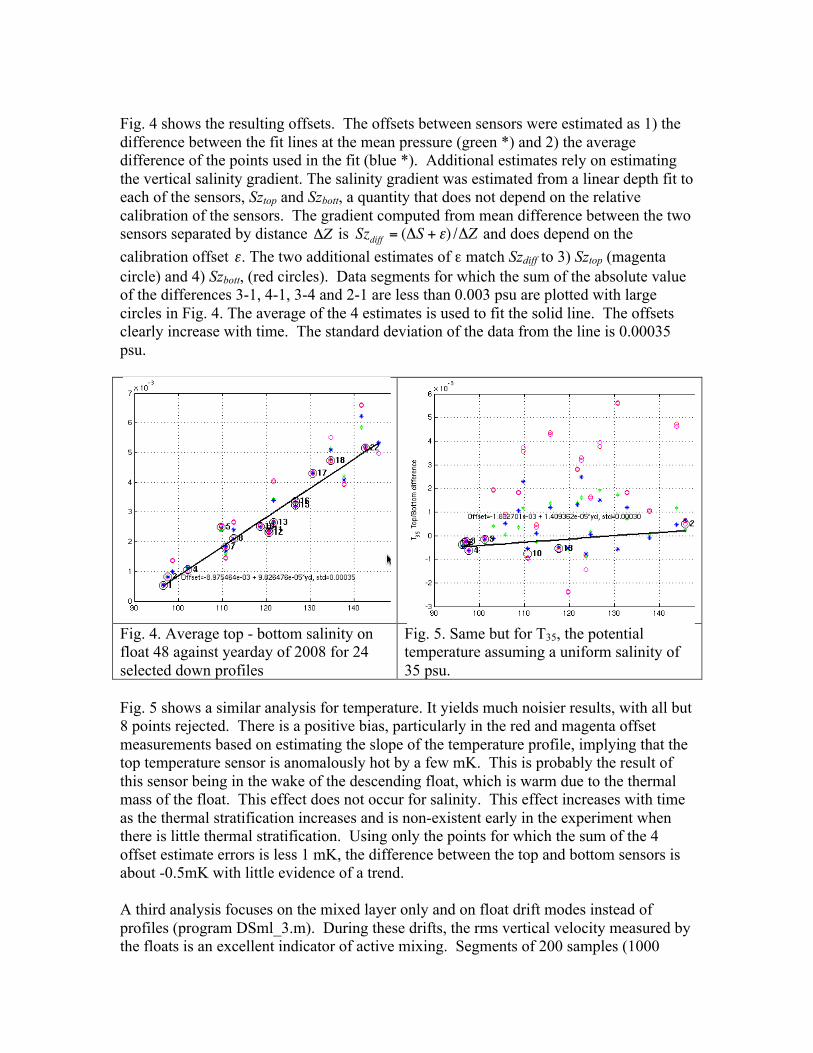
Fig. 4 shows the resulting offsets. The offsets between sensors were estimated as 1) the difference between the fit lines at the mean pressure (green *) and 2) the average difference of the points used in the fit (blue *). Additional estimates rely on estimating the vertical salinity gradient. The salinity gradient was estimated from a linear depth fit to each of the sensors, Sztop and Szbott, a quantity that does not depend on the relative calibration of the sensors. The gradient computed from mean difference between the two sensors separated by distance
€
ΔZ is
€
Szdiff = (ΔS + ε) /ΔZ and does depend on the calibration offset
€
ε. The two additional estimates of ε match Szdiff to 3) Sztop (magenta circle) and 4) Szbott, (red circles). Data segments for which the sum of the absolute value of the differences 3-1, 4-1, 3-4 and 2-1 are less than 0.003 psu are plotted with large circles in Fig. 4. The average of the 4 estimates is used to fit the solid line. The offsets clearly increase with time. The standard deviation of the data from the line is 0.00035 psu.
Fig. 4. Average top - bottom salinity on float 48 against yearday of 2008 for 24 selected down profiles
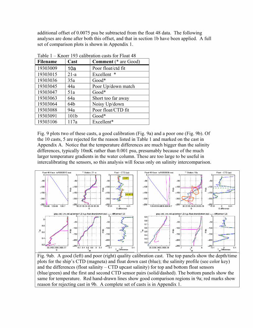
Fig. 5. Same but for T35, the potential temperature assuming a uniform salinity of 35 psu.
Fig. 5 shows a similar analysis for temperature. It yields much noisier results, with all but 8 points rejected. There is a positive bias, particularly in the red and magenta offset measurements based on estimating the slope of the temperature profile, implying that the top temperature sensor is anomalously hot by a few mK. This is probably the result of this sensor being in the wake of the descending float, which is warm due to the thermal mass of the float. This effect does not occur for salinity. This effect increases with time as the thermal stratification increases and is non-existent early in the experiment when there is little thermal stratification. Using only the points for which the sum of the 4 offset estimate errors is less 1 mK, the difference between the top and bottom sensors is about -0.5mK with little evidence of a trend. A third analysis focuses on the mixed layer only and on float drift modes instead of profiles (program DSml_3.m). During these drifts, the rms vertical velocity measured by the floats is an excellent indicator of active mixing. Segments of 200 samples (1000

seconds) were considered well-mixed if the rms vertical velocity was greater than 1 cm s-
1 and at least one data point was shallower than 15m. Fig. 6 shows the mean (o) and median (x) differences between the top and bottom salinities. There is a clear increase in time, slightly less than that in Fig. 4. Fig. 7 shows the same for T35. There is no evidence of a trend and a mean offset of about -0.5 mK.
Fig. 6. Top-bottom salinity difference for float 48 in actively mixing upper mixed layers. Solid line is fit by eye. Dashed is line from Fig. 4.
Fig. 7 Same but for T35,the potential temperature assuming a uniform salinity of 35 psu.
In summary, all three analyses show a trend in the difference between the top and bottom salinities. This can be corrected by adding a linearly increasing offset to the bottom sensor defined by a value of 0.0005 psu at day 97 and a value of 0.005 psu at day 145. There is no evidence of a trend in temperature, but the top sensor reads 0.5mK colder than the bottom on average. These estimates are accurate to better than 0.001 psu and 1mK. The accuracy could probably be increased slightly by a nonlinear fit. These estimates are in addition to an offset 0.007 psu added to the top CTD based on pre-cruise measurements. 1b. Pre and Post Cruise Seabird Calibrations for float 48 Pre-cruise calibrations of the C-T sensors on float 48 were made on Nov. 4, 2007 and July 22, 2007 for sensors 3529 (bottom) and 3530 (top) respectively. Post-cruise calibrations for both sensors were made on Oct. 9, 2008. Fig. 8 shows the difference between computed salinity and temperature using the post-cruise and pre-cruise coefficients for a representative range of temperatures, salinities and pressures (program Seabirdcals.m)

Fig. 8. Difference in computed salinity and temperature between post-cruise and pre-cruise calibration coefficients for the top and bottom CT sensors on float 48. For the top CT sensor (S/N 3530), the temperature differences are somewhat less 1 mK and the salinity differences are somewhat less than 0.001 psu. These changes are small relative to other errors and we will therefore assume that there is no drift in this sensor. For the bottom CTD (S/N 3529), the temperature difference is much less than 1mK. Salinity measurements made using post (pre) cruise calibrations coefficients are about 0.0045 psu saltier (fresher) than those made with pre (post) cruise coefficients. The float data uses the pre-cruise calibrations. This is approximately correct at start of deployment. By the end of the deployment, however, the post-cruise calibrations are more correct and using the pre-cruise calibrations will result in measurements that are too fresh. To bring bottom S into agreement with the more stable top S at the end of the deployment we must therefore add about 0.0045 to bottom S. This agrees with analysis in 1a indicating that a trend needs to be added to the bottom salinity. We will use the trend computed in section 1a to make this correction. 1c. Comparison of float 48 temperature and salinity measurements to those made by the Knorr CTD during the process cruise Knorr cruise 193 carried an SBE-911plus CTD with dual pairs of conductivity and temperature sensors (SN 2774 and 2900 for temperature, 1474 and 1859 for conductivity). Table 1 lists all of the float 48 calibration casts from Knorr 193. As described below, the best match between float 48 and these data requires that an
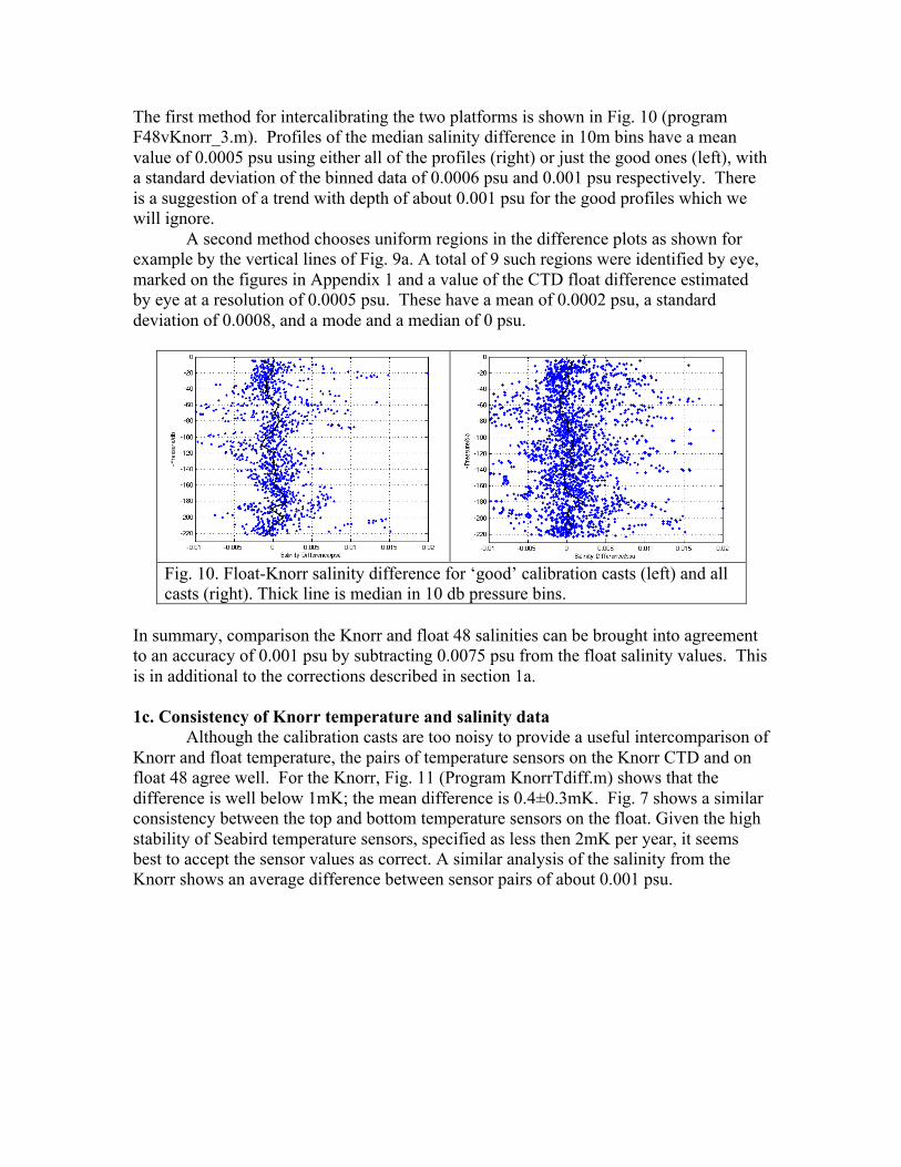
additional offset of 0.0075 psu be subtracted from the float 48 data. The following analyses are done after both this offset, and that in section 1b have been applied. A full set of comparison plots is shown in Appendix 1. Table 1 – Knorr 193 calibration casts for Float 48 Filename Cast Comment (* are Good) 19303009 10a Poor float/ctd fit 19303015 21-a Excellent * 19303036 35a Good* 19303045 44a Poor Up/down match 19303047 51a Good* 19303063 64a Short too far away 19303064 64b Noisy Up/down 19303088 94a Poor float/CTD fit 19303091 101b Good* 19303106 117a Excellent* Fig. 9 plots two of these casts, a good calibration (Fig. 9a) and a poor one (Fig. 9b). Of the 10 casts, 5 are rejected for the reason listed in Table 1 and marked on the cast in Appendix A. Notice that the temperature differences are much bigger than the salinity differences, typically 10mK rather than 0.001 psu, presumably because of the much larger temperature gradients in the water column. These are too large to be useful in intercalibrating the sensors, so this analysis will focus only on salinity intercomparison.
Fig. 9ab. A good (left) and poor (right) quality calibration cast. The top panels show the depth/time plots for the ship’s CTD (magneta) and float down cast (blue); the salinity profile (see color key) and the differences (float salinity – CTD upcast salinity) for top and bottom float sensors (blue/green) and the first and second CTD sensor pairs (solid/dashed). The bottom panels show the same for temperature. Red hand-drawn lines show good comparison regions in 9a; red marks show reason for rejecting cast in 9b. A complete set of casts is in Appendix 1.
The first method for intercalibrating the two platforms is shown in Fig. 10 (program F48vKnorr_3.m). Profiles of the median salinity difference in 10m bins have a mean value of 0.0005 psu using either all of the profiles (right) or just the good ones (left), with a standard deviation of the binned data of 0.0006 psu and 0.001 psu respectively. There is a suggestion of a trend with depth of about 0.001 psu for the good profiles which we will ignore. A second method chooses uniform regions in the difference plots as shown for example by the vertical lines of Fig. 9a. A total of 9 such regions were identified by eye, marked on the figures in Appendix 1 and a value of the CTD float difference estimated by eye at a resolution of 0.0005 psu. These have a mean of 0.0002 psu, a standard deviation of 0.0008, and a mode and a median of 0 psu.
Fig. 10. Float-Knorr salinity difference for ‘good’ calibration casts (left) and all casts (right). Thick line is median in 10 db pressure bins.
In summary, comparison the Knorr and float 48 salinities can be brought into agreement to an accuracy of 0.001 psu by subtracting 0.0075 psu from the float salinity values. This is in additional to the corrections described in section 1a. 1c. Consistency of Knorr temperature and salinity data
Although the calibration casts are too noisy to provide a useful intercomparison of Knorr and float temperature, the pairs of temperature sensors on the Knorr CTD and on float 48 agree well. For the Knorr, Fig. 11 (Program KnorrTdiff.m) shows that the difference is well below 1mK; the mean difference is 0.4±0.3mK. Fig. 7 shows a similar consistency between the top and bottom temperature sensors on the float. Given the high stability of Seabird temperature sensors, specified as less then 2mK per year, it seems best to accept the sensor values as correct. A similar analysis of the salinity from the Knorr shows an average difference between sensor pairs of about 0.001 psu.
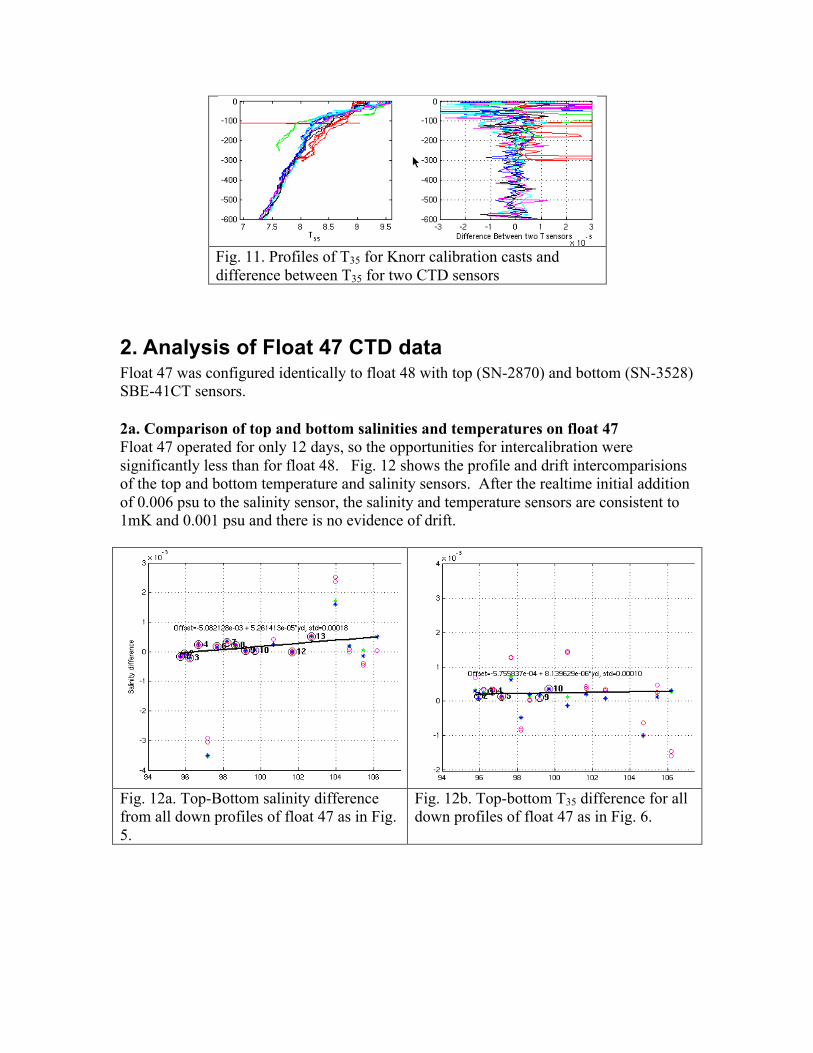
Fig. 11. Profiles of T35 for Knorr calibration casts and difference between T35 for two CTD sensors
2. Analysis of Float 47 CTD data Float 47 was configured identically to float 48 with top (SN-2870) and bottom (SN-3528) SBE-41CT sensors. 2a. Comparison of top and bottom salinities and temperatures on float 47 Float 47 operated for only 12 days, so the opportunities for intercalibration were significantly less than for float 48. Fig. 12 shows the profile and drift intercomparisions of the top and bottom temperature and salinity sensors. After the realtime initial addition of 0.006 psu to the salinity sensor, the salinity and temperature sensors are consistent to 1mK and 0.001 psu and there is no evidence of drift.
Fig. 12a. Top-Bottom salinity difference from all down profiles of float 47 as in Fig. 5.
Fig. 12b. Top-bottom T35 difference for all down profiles of float 47 as in Fig. 6.
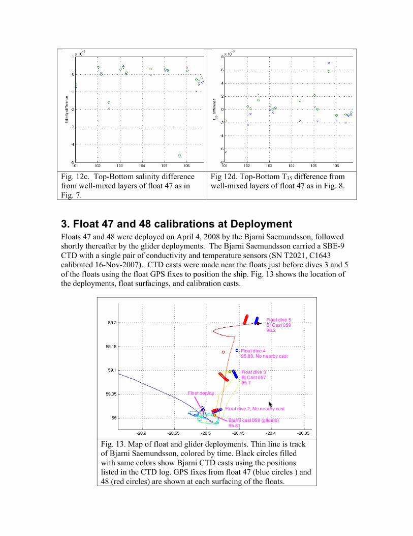
Fig. 12c. Top-Bottom salinity difference from well-mixed layers of float 47 as in Fig. 7.
Fig 12d. Top-Bottom T35 difference from well-mixed layers of float 47 as in Fig. 8.
3. Float 47 and 48 calibrations at Deployment Floats 47 and 48 were deployed on April 4, 2008 by the Bjarni Saemundsson, followed shortly thereafter by the glider deployments. The Bjarni Saemundsson carried a SBE-9 CTD with a single pair of conductivity and temperature sensors (SN T2021, C1643 calibrated 16-Nov-2007). CTD casts were made near the floats just before dives 3 and 5 of the floats using the float GPS fixes to position the ship. Fig. 13 shows the location of the deployments, float surfacings, and calibration casts.
Fig. 13. Map of float and glider deployments. Thin line is track of Bjarni Saemundsson, colored by time. Black circles filled with same colors show Bjarni CTD casts using the positions listed in the CTD log. GPS fixes from float 47 (blue circles ) and 48 (red circles) are shown at each surfacing of the floats.
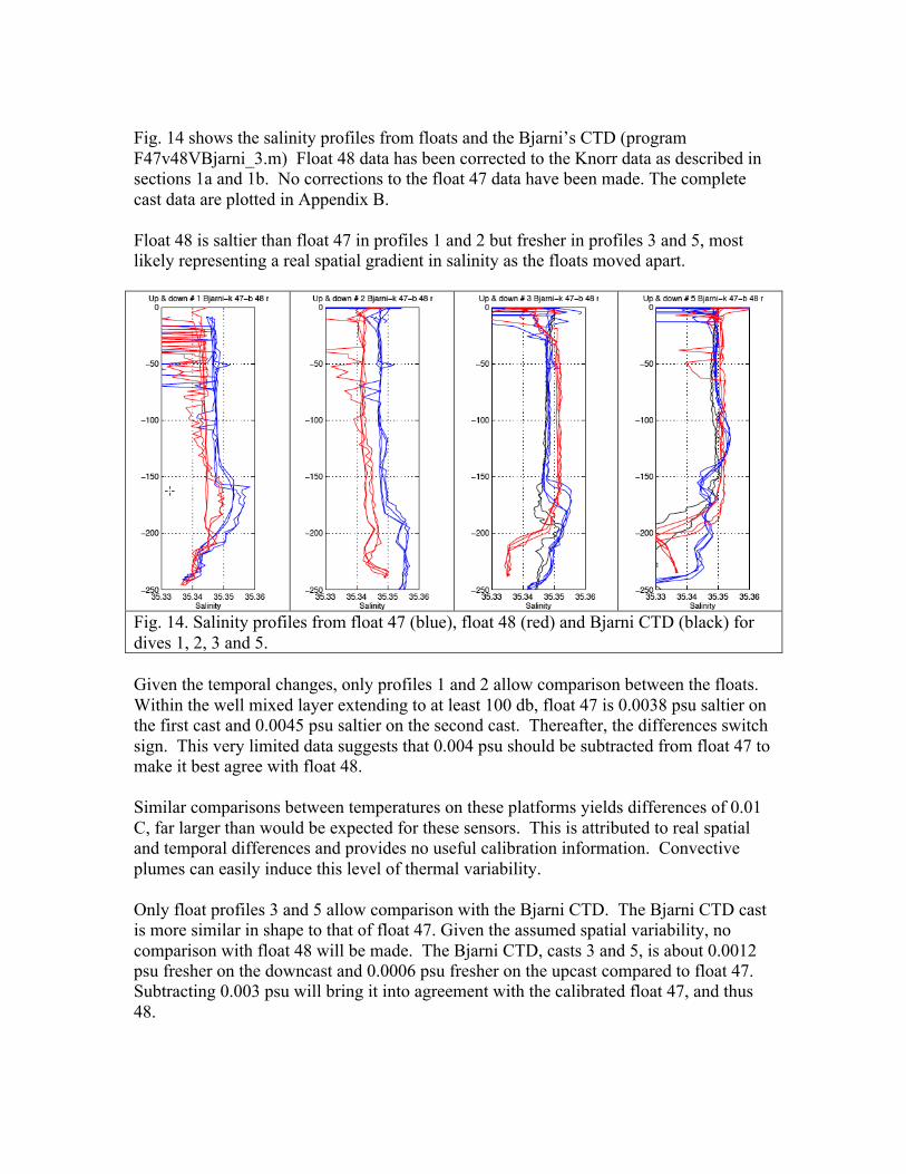
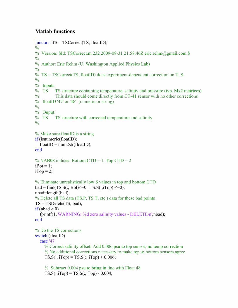
Fig. 14 shows the salinity profiles from floats and the Bjarni’s CTD (program F47v48VBjarni_3.m) Float 48 data has been corrected to the Knorr data as described in sections 1a and 1b. No corrections to the float 47 data have been made. The complete cast data are plotted in Appendix B. Float 48 is saltier than float 47 in profiles 1 and 2 but fresher in profiles 3 and 5, most likely representing a real spatial gradient in salinity as the floats moved apart.
Fig. 14. Salinity profiles from float 47 (blue), float 48 (red) and Bjarni CTD (black) for dives 1, 2, 3 and 5. Given the temporal changes, only profiles 1 and 2 allow comparison between the floats. Within the well mixed layer extending to at least 100 db, float 47 is 0.0038 psu saltier on the first cast and 0.0045 psu saltier on the second cast. Thereafter, the differences switch sign. This very limited data suggests that 0.004 psu should be subtracted from float 47 to make it best agree with float 48. Similar comparisons between temperatures on these platforms yields differences of 0.01 C, far larger than would be expected for these sensors. This is attributed to real spatial and temporal differences and provides no useful calibration information. Convective plumes can easily induce this level of thermal variability. Only float profiles 3 and 5 allow comparison with the Bjarni CTD. The Bjarni CTD cast is more similar in shape to that of float 47. Given the assumed spatial variability, no comparison with float 48 will be made. The Bjarni CTD, casts 3 and 5, is about 0.0012 psu fresher on the downcast and 0.0006 psu fresher on the upcast compared to float 47. Subtracting 0.003 psu will bring it into agreement with the calibrated float 47, and thus 48.

5. Error correction The calibrated sensors still contain errors. Starting with data release v3, measurements with the following conditions were edited: 1. Salinities less than 35 psu. This mostly catches
zero values when the CTD returned no data. 2. Salinity in the top CTD is less than the bottom
CTD by more than 0.03 psu and pressure is less than 4 dbar. Edit the top CTD. This catches times when the top CTD ingests air with the float near the surface.
3. The two CTD’s differ by more than 0.09 psu. Edit the bottom CTD. This catches the worst cases of the error in the bottom CTD described below.
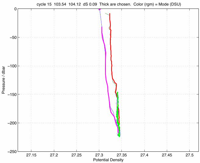
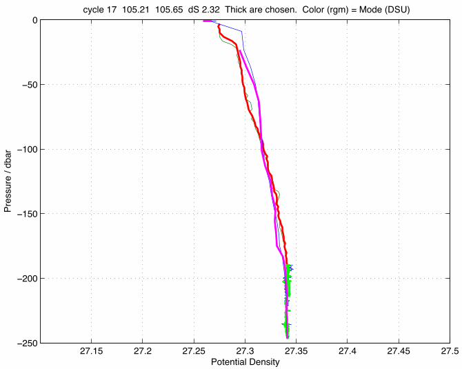
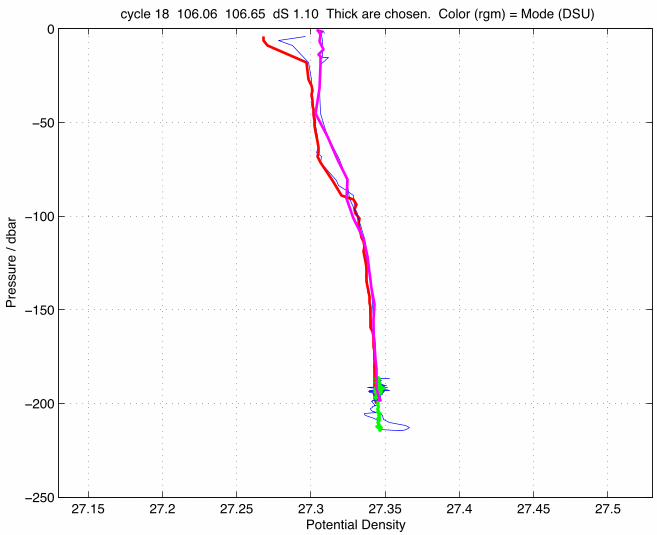
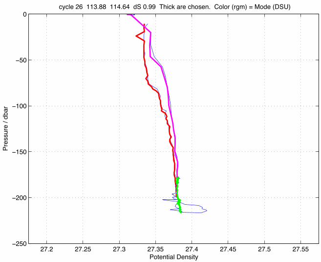
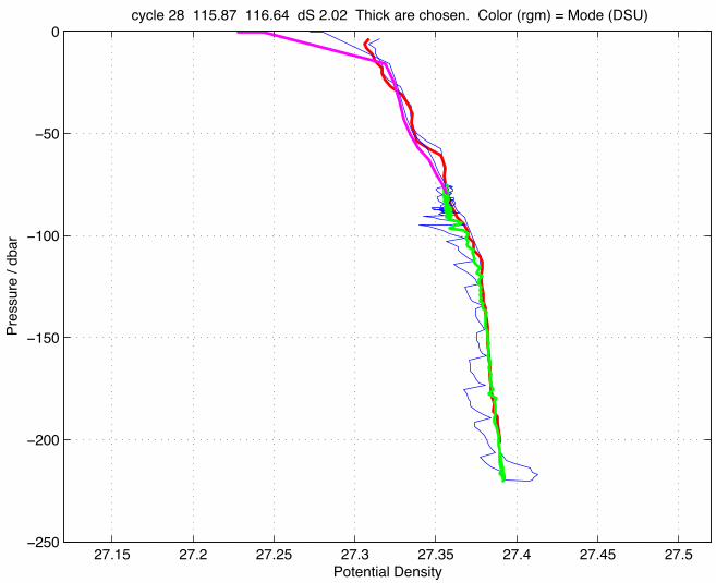
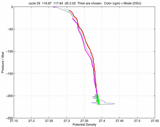
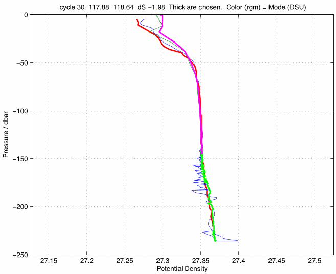
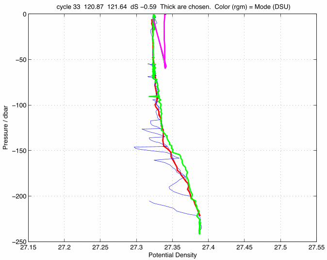
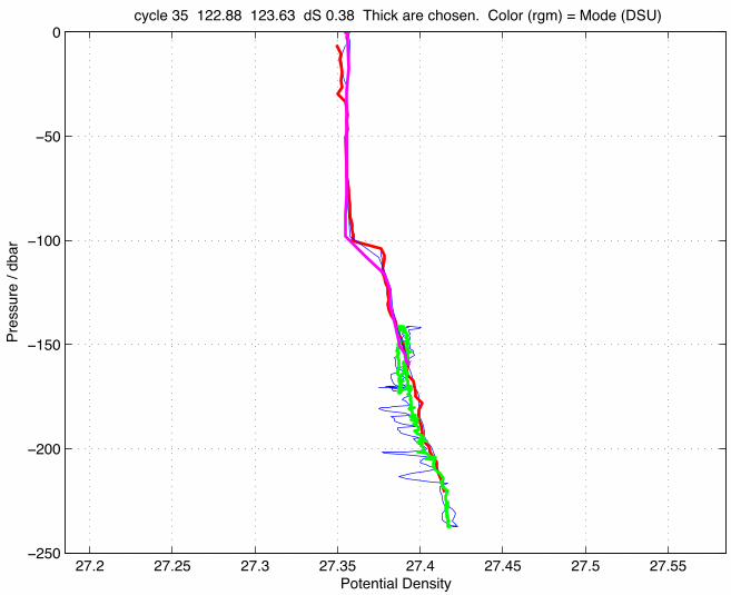
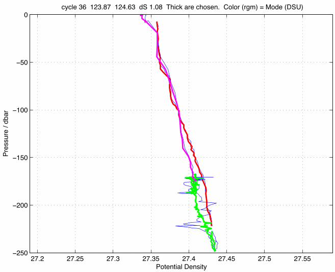
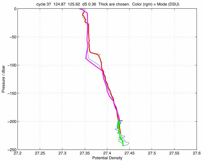
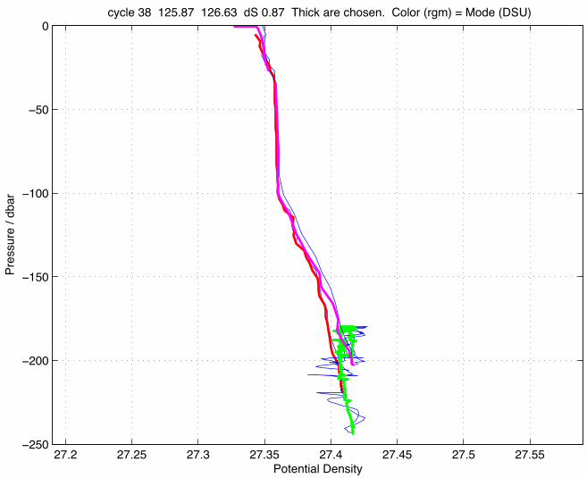
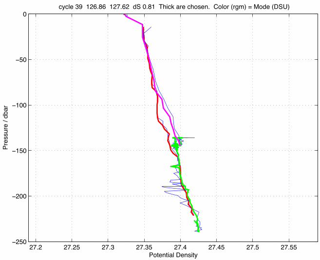
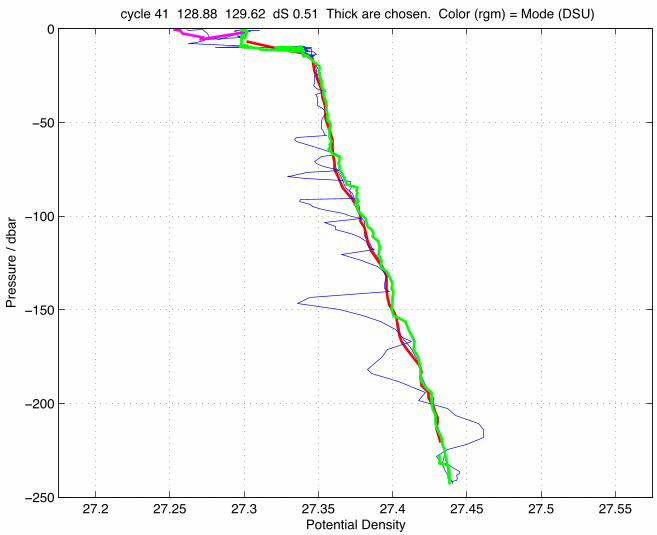
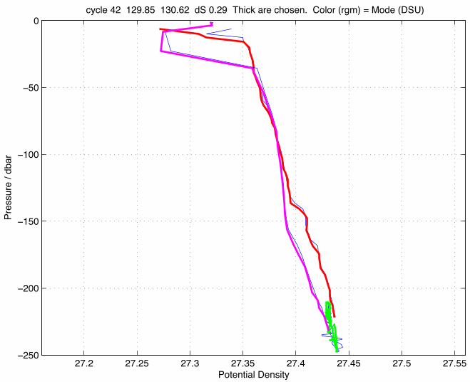
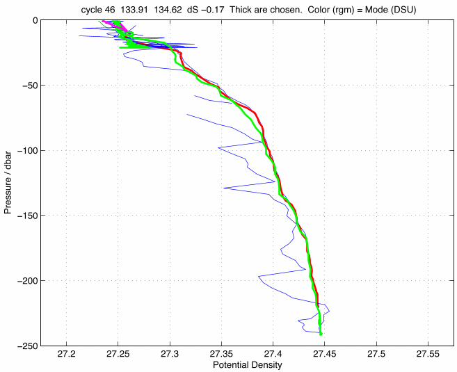
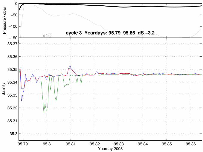
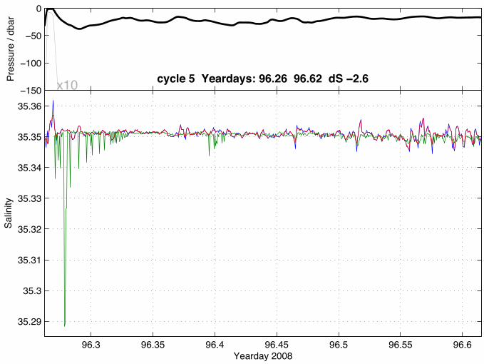
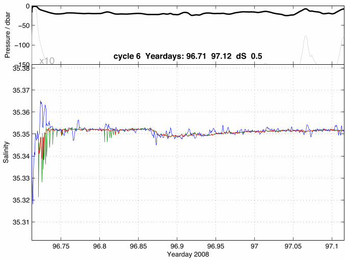
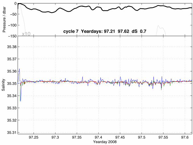
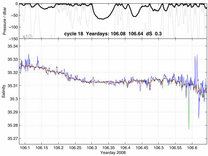
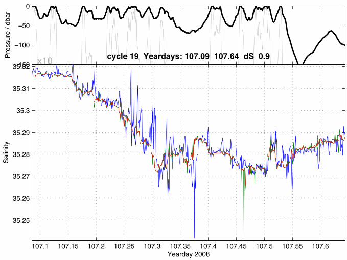
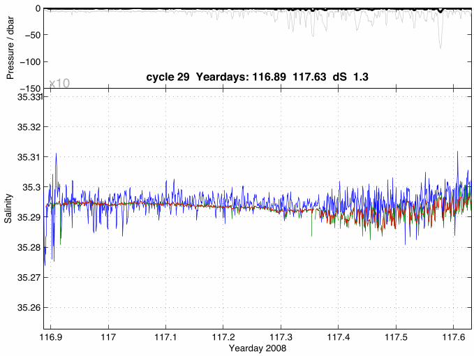
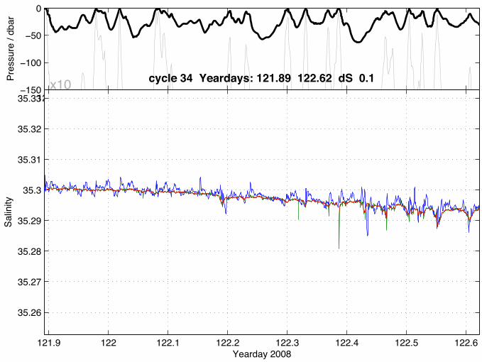
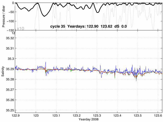
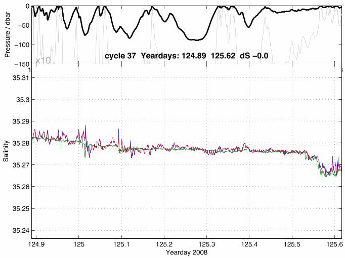
Significant errors in the CTD data remain after these corrections. Figure 15 shows a typical example of high noise and lower values in the bottom CTD consistent with plankton fouling. These errors are sufficiently large that it was decided to merge the two CTD records into a single variable. For each mode of each cycle, the CTD with the smaller standard deviation of salinity was used. A 3 point running median filter was applied to eliminate single spikes. For most of the data, the bottom CTD is noisier than the top CTD. Perhaps the plumbing attached to the sensor reduces the flow rate and prevents plankton flushing. Figures 15 and 16 show examples of the corrected data for profiling and drift modes. Similar figures for the entire data record are shown in Appendices 1 and 2 respectively.
Fig. 15. Example of drift mode salinity data and error correction. Top: Float depth. Bottom: Salinity from top (green) and bottom (blue) sensors. Top sensor is chosen (red).
Fig. 15. Example of error in bottom conductivity sensor (blue) perhaps caused by plankton ingestion. Top CTD (green) looks fine.

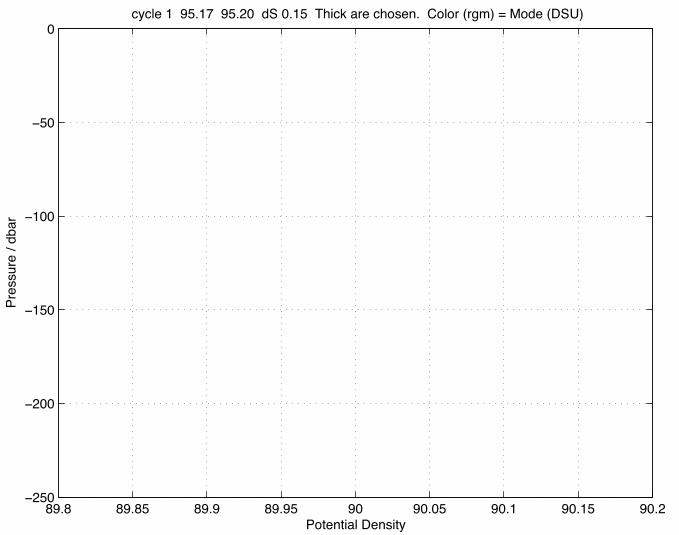
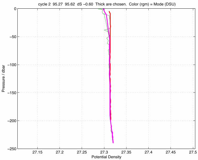
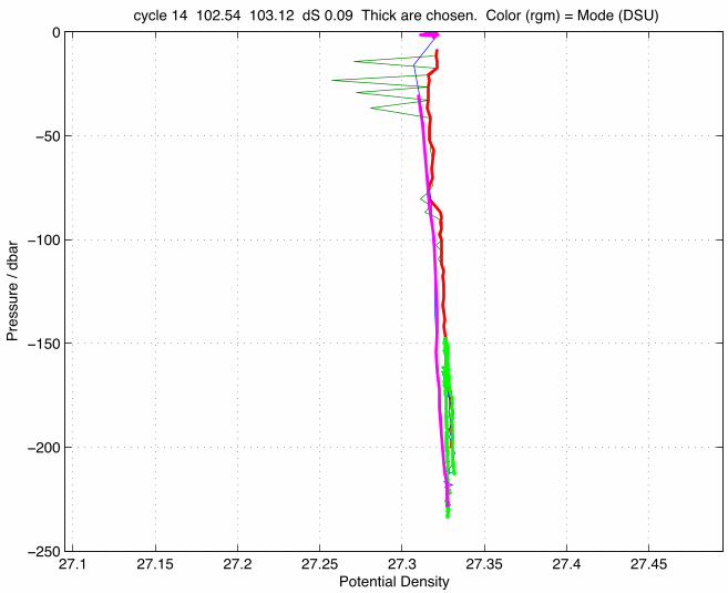
Fig. 16. Example of profile modes error correction. Potential density from bottom (blue) and top (green) sensors is plotted. Algorithm chooses top sensor for down (red) and settle (green) modes and bottom sensorfor up mode (magnenta). Similar plots for all data cycles are included in Appendix I.
6. Conclusions The following recipes bring the following salinity sensors into agreement. Knorr: This is taken as the reference Bjarni deployment: Subtract 0.003psu. This has an uncertainty of several 0.001 psu. Floats 47 and 48: Float 48 can be made to agree with the Knorr CTD during the time of the Knorr cruise. Float 47 can be made to agree with float 48 at deployment. These corrections may well not apply for the second short deployment of float 47. Both corrections are accurate to about 0.001 psu. The Matlab subroutine TSCorrect.m, listed below, applies these calibration corrections to the floats: This is used in releases 3-6 of the float data. The Matlab subroutine ctdchoice.m, listed below, takes this output for float 48 and combines the two temperature and salinity values into a single variable. New variable definitions are: TS.Tcal, TS.Scal – The calibrated values from both top and bottom sensors TS.T, TS.S - The single TS values from choosing between the two sensors TS.ctd - The sensor used in this choice 1=bottom, 2=top TS.Theta, TS.Sig0 – Derived variables from TS.T, TS.S
Matlab functions function TS = TSCorrect(TS, floatID); % % Version: $Id: TSCorrect.m 232 2009-08-31 21:58:46Z [email protected] $ % % Author: Eric Rehm (U. Washington Applied Physics Lab) % % TS = TSCorrect(TS, floatID) does experiment-dependent correction on T, S % % Inputs: % TS TS structure containing temperature, salinity and pressure (typ. Mx2 matrices) % This data should come directly from CT-41 sensor with no other corrections % floatID '47' or '48' (numeric or string) % % Ouput: % TS TS structure with corrected temperature and salinity % % Make sure floatID is a string if (isnumeric(floatID)) floatID = num2str(floatID); end % NAB08 indices: Bottom CTD = 1, Top CTD = 2 iBot = 1; iTop = 2; % Eliminate unrealistically low S values in top and bottom CTD bad = find(TS.S(:,iBot)<=0 | TS.S(:,iTop) <=0); nbad=length(bad); % Delete all TS data (TS.P, TS.T, etc.) data for these bad points TS = TSDelete(TS, bad); if (nbad > 0) fprintf(1,'WARNING: %d zero salinity values - DELETE\n',nbad); end % Do the TS corrections switch (floatID) case '47' % Correct salinity offset: Add 0.006 psu to top sensor; no temp correction % No additional corrections necessary to make top & bottom sensors agree TS.S(:, iTop) = TS.S(:, iTop) + 0.006; % Subtract 0.004 psu to bring in line with Float 48 TS.S(:,iTop) = TS.S(:,iTop) - 0.004;
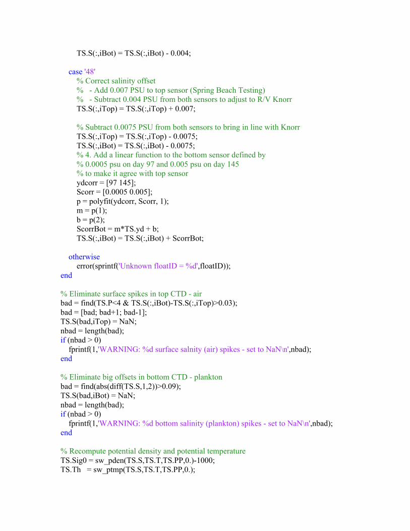
TS.S(:,iBot) = TS.S(:,iBot) - 0.004; case '48' % Correct salinity offset % - Add 0.007 PSU to top sensor (Spring Beach Testing) % - Subtract 0.004 PSU from both sensors to adjust to R/V Knorr TS.S(:,iTop) = TS.S(:,iTop) + 0.007; % Subtract 0.0075 PSU from both sensors to bring in line with Knorr TS.S(:,iTop) = TS.S(:,iTop) - 0.0075; TS.S(:,iBot) = TS.S(:,iBot) - 0.0075; % 4. Add a linear function to the bottom sensor defined by % 0.0005 psu on day 97 and 0.005 psu on day 145 % to make it agree with top sensor ydcorr = [97 145]; Scorr = [0.0005 0.005]; p = polyfit(ydcorr, Scorr, 1); m = p(1); b = p(2); ScorrBot = m*TS.yd + b; TS.S(:,iBot) = TS.S(:,iBot) + ScorrBot; otherwise error(sprintf('Unknown floatID = %d',floatID)); end % Eliminate surface spikes in top CTD - air bad = find(TS.P<4 & TS.S(:,iBot)-TS.S(:,iTop)>0.03); bad = [bad; bad+1; bad-1]; TS.S(bad,iTop) = NaN; nbad = length(bad); if (nbad > 0) fprintf(1,'WARNING: %d surface salnity (air) spikes - set to NaN\n',nbad); end % Eliminate big offsets in bottom CTD - plankton bad = find(abs(diff(TS.S,1,2))>0.09); TS.S(bad,iBot) = NaN; nbad = length(bad); if (nbad > 0) fprintf(1,'WARNING: %d bottom salinity (plankton) spikes - set to NaN\n',nbad); end % Recompute potential density and potential temperature TS.Sig0 = sw_pden(TS.S,TS.T,TS.PP,0.)-1000; TS.Th = sw_ptmp(TS.S,TS.T,TS.PP,0.);
function [TS]=ctdchoice(TS) % Input calibrated CTD data from float 48 % Puts old TS.T TS.S into TS.Tcal TS.Scal % % Makes new TS.T TS.S from best choice of top or bottom CTD % Derived variables TS.Th, TS.Sig0 are computed from these. % New variable TS.ctd = 1 for bottom CTD, 2 for top CTD % % Reads ProfileChoice.mat DriftChoice.mat % Put calibrated dual TS values into new variables TS.Tcal=TS.T; TS.Scal=TS.S; % Make new TS variable by combining these TS.T=TS.T(:,1)*NaN;TS.S=TS.S(:,1)*NaN; drift = load('DriftChoice.mat'); for i=1:length(drift.yd) kk=find(TS.cycle==drift.cycle(i) & TS.mode>2 ); TS.T(kk)=TS.Tcal(kk,drift.ctd(i)); TS.S(kk)=TS.Scal(kk,drift.ctd(i)); TS.ctd(kk)=drift.ctd(i); end prof = load('ProfChoice.mat'); for i=1:length(prof.yd) kk=find(TS.cycle==prof.cycle(i) & TS.mode==prof.mode(i) ); TS.T(kk)=TS.Tcal(kk,prof.ctd(i)); TS.S(kk)=TS.Scal(kk,prof.ctd(i)); TS.ctd(kk)=prof.ctd(i); end TS.Th= sw_ptmp(TS.S,TS.T,TS.P,0.); TS.Sig0=sw_pden(TS.S,TS.T,TS.P,0.)-1000.;

APPENDIX 1 – Profile Mode Error Correction
89.8 89.85 89.9 89.95 90 90.05 90.1 90.15 90.2−250
−200
−150
−100
−50
0
Potential Density
cycle 1 95.17 95.20 dS 0.15 Thick are chosen. Color (rgm) = Mode (DSU)P
ress
ure
/ dba
r
27.15 27.2 27.25 27.3 27.35 27.4 27.45 27.5−250
−200
−150
−100
−50
0
Potential Density
Pre
ssur
e / d
bar
cycle 2 95.27 95.62 dS −0.60 Thick are chosen. Color (rgm) = Mode (DSU)
27.15 27.2 27.25 27.3 27.35 27.4 27.45 27.5−250
−200
−150
−100
−50
0
Potential Density
Pre
ssur
e / d
bar
cycle 3 95.76 95.87 dS −0.07 Thick are chosen. Color (rgm) = Mode (DSU)

27.15 27.2 27.25 27.3 27.35 27.4 27.45 27.5−250
−200
−150
−100
−50
0
Potential Density
Pre
ssur
e / d
bar
cycle 4 95.93 96.12 dS 0.54 Thick are chosen. Color (rgm) = Mode (DSU)

27.15 27.2 27.25 27.3 27.35 27.4 27.45 27.5−250
−200
−150
−100
−50
0
Potential Density
Pre
ssur
e / d
bar
cycle 5 96.24 96.62 dS 0.54 Thick are chosen. Color (rgm) = Mode (DSU)

27.15 27.2 27.25 27.3 27.35 27.4 27.45 27.5−250
−200
−150
−100
−50
0
Potential Density
Pre
ssur
e / d
bar
cycle 6 96.68 97.12 dS −0.09 Thick are chosen. Color (rgm) = Mode (DSU)
27.15 27.2 27.25 27.3 27.35 27.4 27.45 27.5−250
−200
−150
−100
−50
0
Potential Density
Pre
ssur
e / d
bar
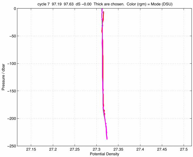
cycle 7 97.19 97.63 dS −0.00 Thick are chosen. Color (rgm) = Mode (DSU)

27.15 27.2 27.25 27.3 27.35 27.4 27.45 27.5−250
−200
−150
−100
−50
0
Potential Density
Pre
ssur
e / d
bar
cycle 8 97.70 98.13 dS 0.46 Thick are chosen. Color (rgm) = Mode (DSU)
27.15 27.2 27.25 27.3 27.35 27.4 27.45 27.5−250
−200
−150
−100
−50
0
Potential Density
Pre
ssur
e / d
bar
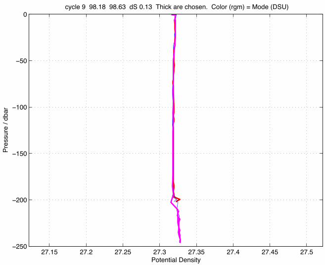
cycle 9 98.18 98.63 dS 0.13 Thick are chosen. Color (rgm) = Mode (DSU)

27.1 27.15 27.2 27.25 27.3 27.35 27.4 27.45−250
−200
−150
−100
−50
0
Potential Density
Pre
ssur
e / d
bar
cycle 10 98.68 99.13 dS 0.37 Thick are chosen. Color (rgm) = Mode (DSU)

27.15 27.2 27.25 27.3 27.35 27.4 27.45 27.5−250
−200
−150
−100
−50
0
Potential Density
Pre
ssur
e / d
bar
cycle 11 99.19 100.13 dS 0.12 Thick are chosen. Color (rgm) = Mode (DSU)

27.15 27.2 27.25 27.3 27.35 27.4 27.45 27.5−250
−200
−150
−100
−50
0
Potential Density
Pre
ssur
e / d
bar
cycle 12 100.20 101.13 dS −0.84 Thick are chosen. Color (rgm) = Mode (DSU)
27.15 27.2 27.25 27.3 27.35 27.4 27.45 27.5−250
−200
−150
−100
−50
0
Potential Density
Pre
ssur
e / d
bar
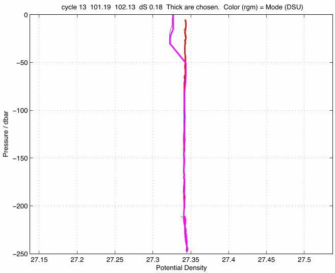
cycle 13 101.19 102.13 dS 0.18 Thick are chosen. Color (rgm) = Mode (DSU)
27.1 27.15 27.2 27.25 27.3 27.35 27.4 27.45−250
−200
−150
−100
−50
0
Potential Density
Pre
ssur
e / d
bar
cycle 14 102.54 103.12 dS 0.09 Thick are chosen. Color (rgm) = Mode (DSU)
27.15 27.2 27.25 27.3 27.35 27.4 27.45 27.5−250
−200
−150
−100
−50
0
Potential Density
Pre
ssur
e / d
bar
cycle 15 103.54 104.12 dS 0.09 Thick are chosen. Color (rgm) = Mode (DSU)

27.15 27.2 27.25 27.3 27.35 27.4 27.45 27.5−250
−200
−150
−100
−50
0
Potential Density
Pre
ssur
e / d
bar
cycle 16 104.72 104.76 dS 7.92 Thick are chosen. Color (rgm) = Mode (DSU)
27.15 27.2 27.25 27.3 27.35 27.4 27.45 27.5−250
−200
−150
−100
−50
0
Potential Density
Pre
ssur
e / d
bar
cycle 17 105.21 105.65 dS 2.32 Thick are chosen. Color (rgm) = Mode (DSU)
27.15 27.2 27.25 27.3 27.35 27.4 27.45 27.5−250
−200
−150
−100
−50
0
Potential Density
Pre
ssur
e / d
bar
cycle 18 106.06 106.65 dS 1.10 Thick are chosen. Color (rgm) = Mode (DSU)

27.15 27.2 27.25 27.3 27.35 27.4 27.45 27.5−250
−200
−150
−100
−50
0
Potential Density
Pre
ssur
e / d
bar
cycle 19 107.07 107.66 dS −0.97 Thick are chosen. Color (rgm) = Mode (DSU)

27.15 27.2 27.25 27.3 27.35 27.4 27.45 27.5−250
−200
−150
−100
−50
0
Potential Density
Pre
ssur
e / d
bar
cycle 20 108.07 108.66 dS −0.50 Thick are chosen. Color (rgm) = Mode (DSU)

27.15 27.2 27.25 27.3 27.35 27.4 27.45 27.5−250
−200
−150
−100
−50
0
Potential Density
Pre
ssur
e / d
bar
cycle 21 109.07 109.65 dS 1.20 Thick are chosen. Color (rgm) = Mode (DSU)

27.15 27.2 27.25 27.3 27.35 27.4 27.45 27.5 27.55−250
−200
−150
−100
−50
0
Potential Density
Pre
ssur
e / d
bar
cycle 22 109.88 110.65 dS −0.16 Thick are chosen. Color (rgm) = Mode (DSU)

27.15 27.2 27.25 27.3 27.35 27.4 27.45 27.5−250
−200
−150
−100
−50
0
Potential Density
Pre
ssur
e / d
bar
cycle 23 110.95 111.65 dS 0.38 Thick are chosen. Color (rgm) = Mode (DSU)

27.15 27.2 27.25 27.3 27.35 27.4 27.45 27.5 27.55−250
−200
−150
−100
−50
0
Potential Density
Pre
ssur
e / d
bar
cycle 24 111.88 112.65 dS 0.90 Thick are chosen. Color (rgm) = Mode (DSU)

27.2 27.25 27.3 27.35 27.4 27.45 27.5 27.55−250
−200
−150
−100
−50
0
Potential Density
Pre
ssur
e / d
bar
cycle 25 112.88 113.64 dS 1.65 Thick are chosen. Color (rgm) = Mode (DSU)
27.2 27.25 27.3 27.35 27.4 27.45 27.5 27.55−250
−200
−150
−100
−50
0
Potential Density
Pre
ssur
e / d
bar
cycle 26 113.88 114.64 dS 0.99 Thick are chosen. Color (rgm) = Mode (DSU)

27.2 27.25 27.3 27.35 27.4 27.45 27.5 27.55−250
−200
−150
−100
−50
0
Potential Density
Pre
ssur
e / d
bar
cycle 27 114.87 115.64 dS 1.99 Thick are chosen. Color (rgm) = Mode (DSU)
27.15 27.2 27.25 27.3 27.35 27.4 27.45 27.5−250
−200
−150
−100
−50
0
Potential Density
Pre
ssur
e / d
bar
cycle 28 115.87 116.64 dS 2.02 Thick are chosen. Color (rgm) = Mode (DSU)
27.15 27.2 27.25 27.3 27.35 27.4 27.45 27.5 27.55−250
−200
−150
−100
−50
0
Potential Density
Pre
ssur
e / d
bar
cycle 29 116.87 117.64 dS 2.02 Thick are chosen. Color (rgm) = Mode (DSU)
27.15 27.2 27.25 27.3 27.35 27.4 27.45 27.5−250
−200
−150
−100
−50
0
Potential Density
Pre
ssur
e / d
bar
cycle 30 117.88 118.64 dS −1.98 Thick are chosen. Color (rgm) = Mode (DSU)

27.15 27.2 27.25 27.3 27.35 27.4 27.45 27.5−250
−200
−150
−100
−50
0
Potential Density
Pre
ssur
e / d
bar
cycle 31 118.87 119.64 dS −2.22 Thick are chosen. Color (rgm) = Mode (DSU)

27.15 27.2 27.25 27.3 27.35 27.4 27.45 27.5−250
−200
−150
−100
−50
0
Potential Density
Pre
ssur
e / d
bar
cycle 32 119.87 120.64 dS −0.17 Thick are chosen. Color (rgm) = Mode (DSU)
27.15 27.2 27.25 27.3 27.35 27.4 27.45 27.5 27.55−250
−200
−150
−100
−50
0
Potential Density
Pre
ssur
e / d
bar
cycle 33 120.87 121.64 dS −0.59 Thick are chosen. Color (rgm) = Mode (DSU)

27.2 27.25 27.3 27.35 27.4 27.45 27.5 27.55−250
−200
−150
−100
−50
0
Potential Density
Pre
ssur
e / d
bar
cycle 34 121.87 122.63 dS 1.13 Thick are chosen. Color (rgm) = Mode (DSU)
27.2 27.25 27.3 27.35 27.4 27.45 27.5 27.55−250
−200
−150
−100
−50
0
Potential Density
Pre
ssur
e / d
bar
cycle 35 122.88 123.63 dS 0.38 Thick are chosen. Color (rgm) = Mode (DSU)
27.2 27.25 27.3 27.35 27.4 27.45 27.5 27.55−250
−200
−150
−100
−50
0
Potential Density
Pre
ssur
e / d
bar
cycle 36 123.87 124.63 dS 1.08 Thick are chosen. Color (rgm) = Mode (DSU)
27.2 27.25 27.3 27.35 27.4 27.45 27.5 27.55 27.6−250
−200
−150
−100
−50
0
Potential Density
Pre
ssur
e / d
bar
cycle 37 124.87 125.62 dS 0.36 Thick are chosen. Color (rgm) = Mode (DSU)
27.2 27.25 27.3 27.35 27.4 27.45 27.5 27.55−250
−200
−150
−100
−50
0
Potential Density
Pre
ssur
e / d
bar
cycle 38 125.87 126.63 dS 0.87 Thick are chosen. Color (rgm) = Mode (DSU)
27.2 27.25 27.3 27.35 27.4 27.45 27.5 27.55−250
−200
−150
−100
−50
0
Potential Density
Pre
ssur
e / d
bar
cycle 39 126.86 127.62 dS 0.81 Thick are chosen. Color (rgm) = Mode (DSU)

27.2 27.25 27.3 27.35 27.4 27.45 27.5 27.55−250
−200
−150
−100
−50
0
Potential Density
Pre
ssur
e / d
bar
cycle 40 127.86 128.62 dS 1.42 Thick are chosen. Color (rgm) = Mode (DSU)
27.2 27.25 27.3 27.35 27.4 27.45 27.5 27.55−250
−200
−150
−100
−50
0
Potential Density
Pre
ssur
e / d
bar
cycle 41 128.88 129.62 dS 0.51 Thick are chosen. Color (rgm) = Mode (DSU)
27.2 27.25 27.3 27.35 27.4 27.45 27.5 27.55−250
−200
−150
−100
−50
0
Potential Density
Pre
ssur
e / d
bar
cycle 42 129.85 130.62 dS 0.29 Thick are chosen. Color (rgm) = Mode (DSU)

27.2 27.25 27.3 27.35 27.4 27.45 27.5 27.55−250
−200
−150
−100
−50
0
Potential Density
Pre
ssur
e / d
bar
cycle 43 130.87 131.62 dS 3.89 Thick are chosen. Color (rgm) = Mode (DSU)

27.2 27.25 27.3 27.35 27.4 27.45 27.5 27.55−250
−200
−150
−100
−50
0
Potential Density
Pre
ssur
e / d
bar
cycle 44 131.87 132.62 dS 0.01 Thick are chosen. Color (rgm) = Mode (DSU)

27.2 27.25 27.3 27.35 27.4 27.45 27.5 27.55−250
−200
−150
−100
−50
0
Potential Density
Pre
ssur
e / d
bar
cycle 45 132.91 133.62 dS 0.95 Thick are chosen. Color (rgm) = Mode (DSU)
27.2 27.25 27.3 27.35 27.4 27.45 27.5 27.55−250
−200
−150
−100
−50
0
Potential Density
Pre
ssur
e / d
bar
cycle 46 133.91 134.62 dS −0.17 Thick are chosen. Color (rgm) = Mode (DSU)

27.2 27.25 27.3 27.35 27.4 27.45 27.5 27.55−250
−200
−150
−100
−50
0
Potential Density
Pre
ssur
e / d
bar
cycle 47 134.89 135.63 dS 0.80 Thick are chosen. Color (rgm) = Mode (DSU)

27.2 27.25 27.3 27.35 27.4 27.45 27.5 27.55−250
−200
−150
−100
−50
0
Potential Density
Pre
ssur
e / d
bar
cycle 48 135.87 136.62 dS 1.71 Thick are chosen. Color (rgm) = Mode (DSU)

27.2 27.25 27.3 27.35 27.4 27.45 27.5 27.55−250
−200
−150
−100
−50
0
Potential Density
Pre
ssur
e / d
bar
cycle 49 136.92 137.63 dS 3.62 Thick are chosen. Color (rgm) = Mode (DSU)
27.2 27.25 27.3 27.35 27.4 27.45 27.5 27.55−250
−200
−150
−100
−50
0
Potential Density
Pre
ssur
e / d
bar
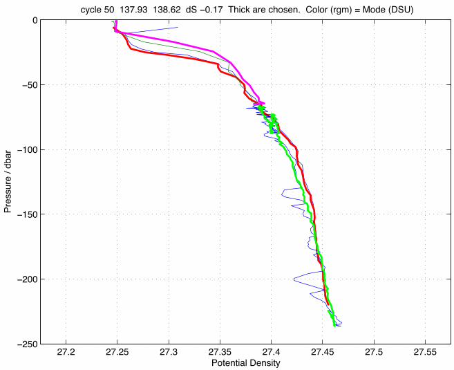
cycle 50 137.93 138.62 dS −0.17 Thick are chosen. Color (rgm) = Mode (DSU)
27.2 27.25 27.3 27.35 27.4 27.45 27.5 27.55−250
−200
−150
−100
−50
0
Potential Density
Pre
ssur
e / d
bar
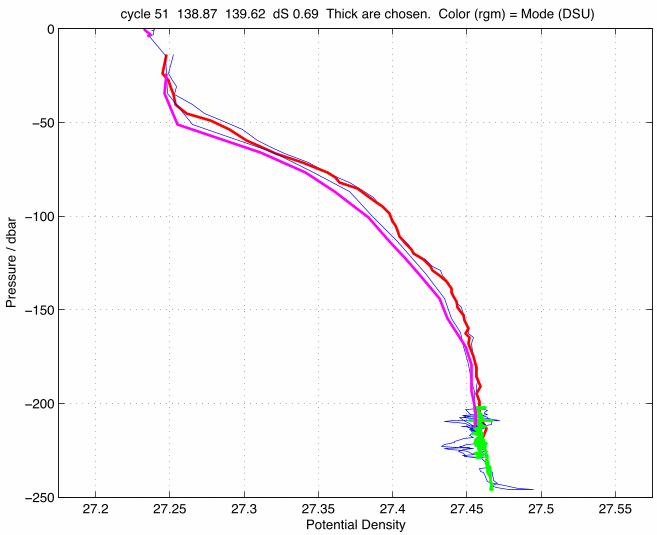
cycle 51 138.87 139.62 dS 0.69 Thick are chosen. Color (rgm) = Mode (DSU)

27.2 27.25 27.3 27.35 27.4 27.45 27.5 27.55 27.6−250
−200
−150
−100
−50
0
Potential Density
Pre
ssur
e / d
bar
cycle 52 139.90 140.63 dS 1.88 Thick are chosen. Color (rgm) = Mode (DSU)
27.2 27.25 27.3 27.35 27.4 27.45 27.5 27.55−250
−200
−150
−100
−50
0
Potential Density
Pre
ssur
e / d
bar
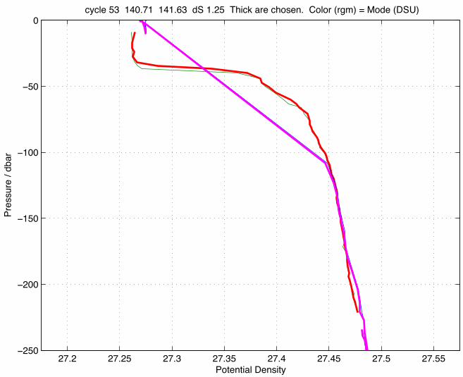
cycle 53 140.71 141.63 dS 1.25 Thick are chosen. Color (rgm) = Mode (DSU)

27.2 27.25 27.3 27.35 27.4 27.45 27.5 27.55−250
−200
−150
−100
−50
0
Potential Density
Pre
ssur
e / d
bar
cycle 54 141.79 142.63 dS 0.06 Thick are chosen. Color (rgm) = Mode (DSU)

27.2 27.25 27.3 27.35 27.4 27.45 27.5 27.55−250
−200
−150
−100
−50
0
Potential Density
Pre
ssur
e / d
bar
cycle 55 142.71 143.64 dS −0.08 Thick are chosen. Color (rgm) = Mode (DSU)

27.2 27.25 27.3 27.35 27.4 27.45 27.5 27.55 27.6−250
−200
−150
−100
−50
0
Potential Density
Pre
ssur
e / d
bar
cycle 56 143.89 144.67 dS −2.07 Thick are chosen. Color (rgm) = Mode (DSU)

27.2 27.25 27.3 27.35 27.4 27.45 27.5 27.55−250
−200
−150
−100
−50
0
Potential Density
Pre
ssur
e / d
bar
cycle 57 144.95 145.67 dS −1.36 Thick are chosen. Color (rgm) = Mode (DSU)
27.2 27.25 27.3 27.35 27.4 27.45 27.5 27.55−250
−200
−150
−100
−50
0
Potential Density
Pre
ssur
e / d
bar
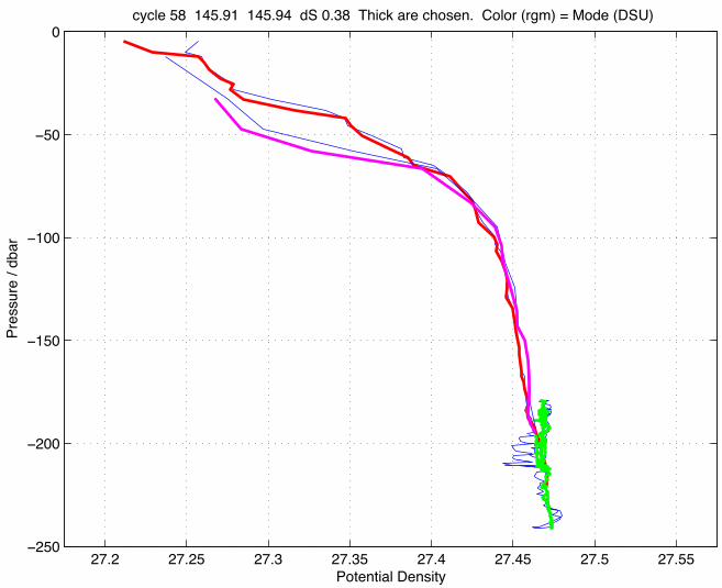
cycle 58 145.91 145.94 dS 0.38 Thick are chosen. Color (rgm) = Mode (DSU)

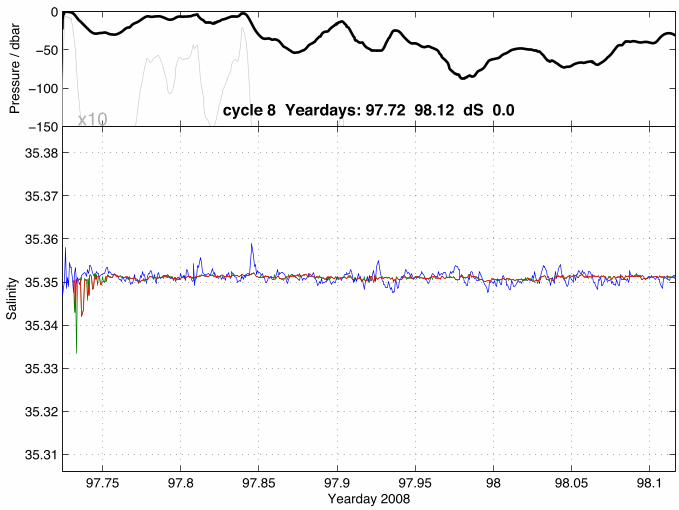
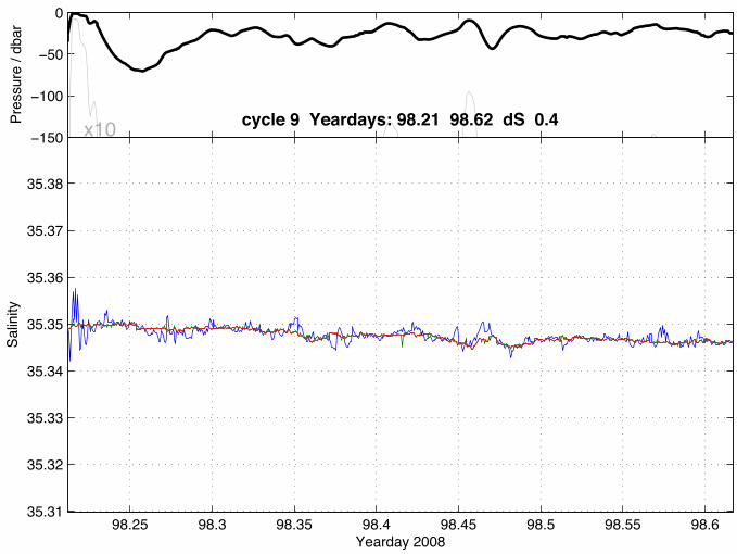
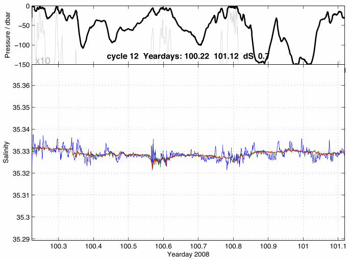
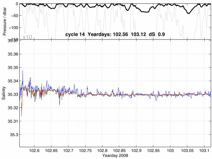
APPENDIX 2 – Drift Mode Error Correction

95.3 95.35 95.4 95.45 95.5 95.55 95.6−150
−100
−50
0
x10
Pre
ssur
e / d
bar
95.3 95.35 95.4 95.45 95.5 95.55 95.6
35.31
35.32
35.33
35.34
35.35
35.36
35.37
35.38
Sal
inity
Yearday 2008
cycle 2 Yeardays: 95.29 95.61 dS 0.6
95.79 95.8 95.81 95.82 95.83 95.84 95.85 95.86−150
−100
−50
0
x10
Pre
ssur
e / d
bar
95.79 95.8 95.81 95.82 95.83 95.84 95.85 95.86
35.3
35.31
35.32
35.33
35.34
35.35
35.36
35.37
Sal
inity
Yearday 2008
cycle 3 Yeardays: 95.79 95.86 dS −3.2

95.96 95.98 96 96.02 96.04 96.06 96.08 96.1−150
−100
−50
0
x10
Pre
ssur
e / d
bar
95.96 95.98 96 96.02 96.04 96.06 96.08 96.1
35.31
35.32
35.33
35.34
35.35
35.36
35.37
35.38
Sal
inity
Yearday 2008
cycle 4 Yeardays: 95.96 96.12 dS 0.6
96.3 96.35 96.4 96.45 96.5 96.55 96.6−150
−100
−50
0
x10
Pre
ssur
e / d
bar
96.3 96.35 96.4 96.45 96.5 96.55 96.6
35.29
35.3
35.31
35.32
35.33
35.34
35.35
35.36
Sal
inity
Yearday 2008
cycle 5 Yeardays: 96.26 96.62 dS −2.6
96.75 96.8 96.85 96.9 96.95 97 97.05 97.1−150
−100
−50
0
x10
Pre
ssur
e / d
bar
96.75 96.8 96.85 96.9 96.95 97 97.05 97.1
35.31
35.32
35.33
35.34
35.35
35.36
35.37
35.38
Sal
inity
Yearday 2008
cycle 6 Yeardays: 96.71 97.12 dS 0.5
97.25 97.3 97.35 97.4 97.45 97.5 97.55 97.6−150
−100
−50
0
x10
Pre
ssur
e / d
bar
97.25 97.3 97.35 97.4 97.45 97.5 97.55 97.635.31
35.32
35.33
35.34
35.35
35.36
35.37
35.38
Sal
inity
Yearday 2008
cycle 7 Yeardays: 97.21 97.62 dS 0.7
97.75 97.8 97.85 97.9 97.95 98 98.05 98.1−150
−100
−50
0
x10
Pre
ssur
e / d
bar
97.75 97.8 97.85 97.9 97.95 98 98.05 98.1
35.31
35.32
35.33
35.34
35.35
35.36
35.37
35.38
Sal
inity
Yearday 2008
cycle 8 Yeardays: 97.72 98.12 dS 0.0
98.25 98.3 98.35 98.4 98.45 98.5 98.55 98.6−150
−100
−50
0
x10
Pre
ssur
e / d
bar
98.25 98.3 98.35 98.4 98.45 98.5 98.55 98.635.31
35.32
35.33
35.34
35.35
35.36
35.37
35.38
Sal
inity
Yearday 2008
cycle 9 Yeardays: 98.21 98.62 dS 0.4

98.75 98.8 98.85 98.9 98.95 99 99.05 99.1−150
−100
−50
0
x10
Pre
ssur
e / d
bar
98.75 98.8 98.85 98.9 98.95 99 99.05 99.1
35.31
35.32
35.33
35.34
35.35
35.36
35.37
35.38
Sal
inity
Yearday 2008
cycle 10 Yeardays: 98.71 99.12 dS 0.7

99.3 99.4 99.5 99.6 99.7 99.8 99.9 100 100.1−150
−100
−50
0
x10
Pre
ssur
e / d
bar
99.3 99.4 99.5 99.6 99.7 99.8 99.9 100 100.1
35.31
35.32
35.33
35.34
35.35
35.36
35.37
35.38
Sal
inity
Yearday 2008
cycle 11 Yeardays: 99.21 100.12 dS 1.2
100.3 100.4 100.5 100.6 100.7 100.8 100.9 101 101.1−150
−100
−50
0
x10
Pre
ssur
e / d
bar
100.3 100.4 100.5 100.6 100.7 100.8 100.9 101 101.135.29
35.3
35.31
35.32
35.33
35.34
35.35
35.36
Sal
inity
Yearday 2008
cycle 12 Yeardays: 100.22 101.12 dS 0.7

101.3 101.4 101.5 101.6 101.7 101.8 101.9 102 102.1−150
−100
−50
0
x10
Pre
ssur
e / d
bar
101.3 101.4 101.5 101.6 101.7 101.8 101.9 102 102.1
35.3
35.31
35.32
35.33
35.34
35.35
35.36
35.37
Sal
inity
Yearday 2008
cycle 13 Yeardays: 101.22 102.12 dS 1.0
102.6 102.65 102.7 102.75 102.8 102.85 102.9 102.95 103 103.05 103.1−150
−100
−50
0
x10
Pre
ssur
e / d
bar
102.6 102.65 102.7 102.75 102.8 102.85 102.9 102.95 103 103.05 103.1
35.3
35.31
35.32
35.33
35.34
35.35
35.36
35.37
Sal
inity
Yearday 2008
cycle 14 Yeardays: 102.56 103.12 dS 0.9

103.6 103.65 103.7 103.75 103.8 103.85 103.9 103.95 104 104.05 104.1−150
−100
−50
0
x10
Pre
ssur
e / d
bar
103.6 103.65 103.7 103.75 103.8 103.85 103.9 103.95 104 104.05 104.1
35.29
35.3
35.31
35.32
35.33
35.34
35.35
35.36
Sal
inity
Yearday 2008
cycle 15 Yeardays: 103.55 104.12 dS 0.9

105.25 105.3 105.35 105.4 105.45 105.5 105.55 105.6−150
−100
−50
0
x10
Pre
ssur
e / d
bar
105.25 105.3 105.35 105.4 105.45 105.5 105.55 105.6
35.29
35.3
35.31
35.32
35.33
35.34
35.35
35.36
Sal
inity
Yearday 2008
cycle 17 Yeardays: 105.23 105.64 dS 1.7
106.1 106.15 106.2 106.25 106.3 106.35 106.4 106.45 106.5 106.55 106.6−150
−100
−50
0
x10
Pre
ssur
e / d
bar
106.1 106.15 106.2 106.25 106.3 106.35 106.4 106.45 106.5 106.55 106.6
35.27
35.28
35.29
35.3
35.31
35.32
35.33
35.34
Sal
inity
Yearday 2008
cycle 18 Yeardays: 106.08 106.64 dS 0.3
107.1 107.15 107.2 107.25 107.3 107.35 107.4 107.45 107.5 107.55 107.6−150
−100
−50
0
x10
Pre
ssur
e / d
bar
107.1 107.15 107.2 107.25 107.3 107.35 107.4 107.45 107.5 107.55 107.6
35.25
35.26
35.27
35.28
35.29
35.3
35.31
35.32
Sal
inity
Yearday 2008
cycle 19 Yeardays: 107.09 107.64 dS 0.9

108.1 108.15 108.2 108.25 108.3 108.35 108.4 108.45 108.5 108.55 108.6−150
−100
−50
0
x10
Pre
ssur
e / d
bar
108.1 108.15 108.2 108.25 108.3 108.35 108.4 108.45 108.5 108.55 108.6
35.26
35.27
35.28
35.29
35.3
35.31
35.32
35.33
Sal
inity
Yearday 2008
cycle 20 Yeardays: 108.09 108.64 dS 0.2
109.1 109.15 109.2 109.25 109.3 109.35 109.4 109.45 109.5 109.55 109.6−150
−100
−50
0
x10
Pre
ssur
e / d
bar
109.1 109.15 109.2 109.25 109.3 109.35 109.4 109.45 109.5 109.55 109.6
35.28
35.29
35.3
35.31
35.32
35.33
35.34
35.35
Sal
inity
Yearday 2008
cycle 21 Yeardays: 109.10 109.65 dS −0.0
109.9 110 110.1 110.2 110.3 110.4 110.5 110.6−150
−100
−50
0
x10
Pre
ssur
e / d
bar
109.9 110 110.1 110.2 110.3 110.4 110.5 110.6
35.27
35.28
35.29
35.3
35.31
35.32
35.33
35.34
Sal
inity
Yearday 2008
cycle 22 Yeardays: 109.90 110.64 dS −0.4
111 111.1 111.2 111.3 111.4 111.5 111.6−150
−100
−50
0
x10
Pre
ssur
e / d
bar
111 111.1 111.2 111.3 111.4 111.5 111.6
35.25
35.26
35.27
35.28
35.29
35.3
35.31
35.32
Sal
inity
Yearday 2008
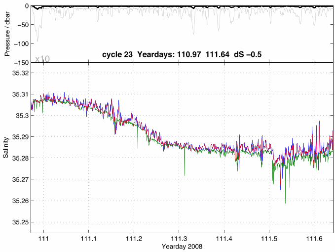
cycle 23 Yeardays: 110.97 111.64 dS −0.5

111.9 112 112.1 112.2 112.3 112.4 112.5 112.6−150
−100
−50
0
x10
Pre
ssur
e / d
bar
111.9 112 112.1 112.2 112.3 112.4 112.5 112.6
35.25
35.26
35.27
35.28
35.29
35.3
35.31
35.32
Sal
inity
Yearday 2008
cycle 24 Yeardays: 111.90 112.64 dS 1.2
113 113.1 113.2 113.3 113.4 113.5 113.6−150
−100
−50
0
x10
Pre
ssur
e / d
bar
113 113.1 113.2 113.3 113.4 113.5 113.6
35.26
35.27
35.28
35.29
35.3
35.31
35.32
35.33
Sal
inity
Yearday 2008
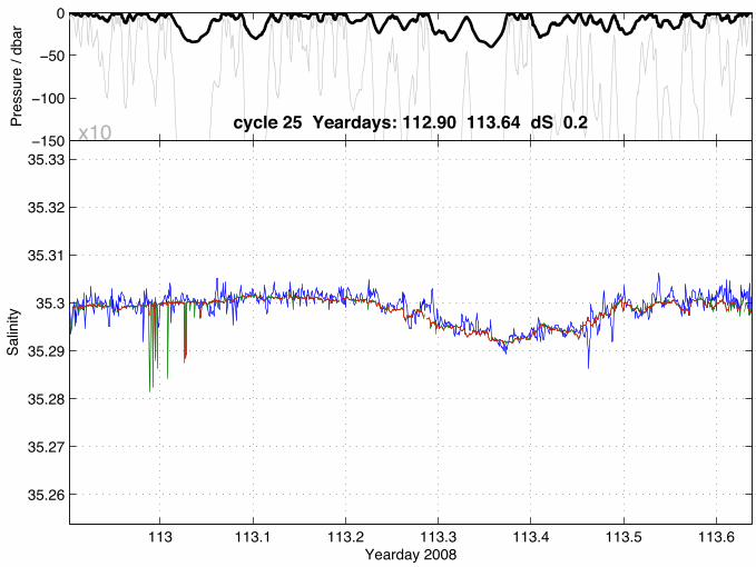
cycle 25 Yeardays: 112.90 113.64 dS 0.2

113.9 114 114.1 114.2 114.3 114.4 114.5 114.6−150
−100
−50
0
x10
Pre
ssur
e / d
bar
113.9 114 114.1 114.2 114.3 114.4 114.5 114.6
35.24
35.25
35.26
35.27
35.28
35.29
35.3
35.31
Sal
inity
Yearday 2008
cycle 26 Yeardays: 113.89 114.64 dS −0.5
114.9 115 115.1 115.2 115.3 115.4 115.5 115.6−150
−100
−50
0
x10
Pre
ssur
e / d
bar
114.9 115 115.1 115.2 115.3 115.4 115.5 115.6
35.25
35.26
35.27
35.28
35.29
35.3
35.31
35.32
Sal
inity
Yearday 2008
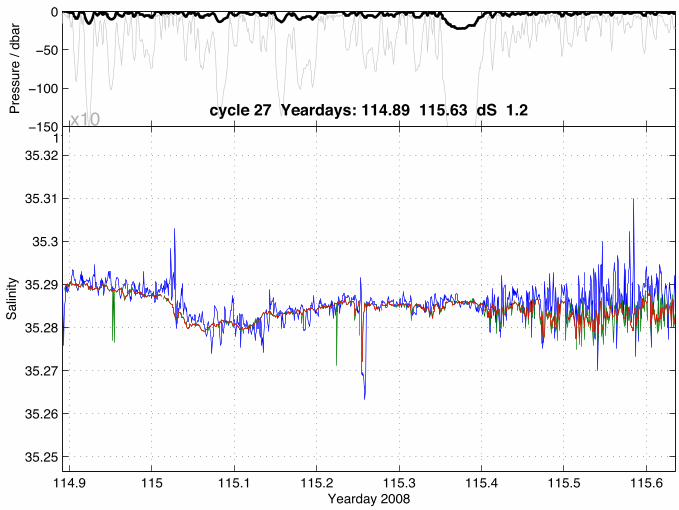
cycle 27 Yeardays: 114.89 115.63 dS 1.2
115.9 116 116.1 116.2 116.3 116.4 116.5 116.6−150
−100
−50
0
x10
Pre
ssur
e / d
bar
115.9 116 116.1 116.2 116.3 116.4 116.5 116.6
35.26
35.27
35.28
35.29
35.3
35.31
35.32
35.33
Sal
inity
Yearday 2008
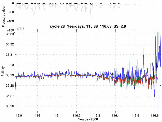
cycle 28 Yeardays: 115.88 116.63 dS 2.9
116.9 117 117.1 117.2 117.3 117.4 117.5 117.6−150
−100
−50
0
x10
Pre
ssur
e / d
bar
116.9 117 117.1 117.2 117.3 117.4 117.5 117.6
35.26
35.27
35.28
35.29
35.3
35.31
35.32
35.33
Sal
inity
Yearday 2008
cycle 29 Yeardays: 116.89 117.63 dS 1.3

117.9 118 118.1 118.2 118.3 118.4 118.5 118.6−150
−100
−50
0
x10
Pre
ssur
e / d
bar
117.9 118 118.1 118.2 118.3 118.4 118.5 118.635.26
35.27
35.28
35.29
35.3
35.31
35.32
35.33
Sal
inity
Yearday 2008
cycle 30 Yeardays: 117.90 118.63 dS 1.1

118.9 119 119.1 119.2 119.3 119.4 119.5 119.6−150
−100
−50
0
x10
Pre
ssur
e / d
bar
118.9 119 119.1 119.2 119.3 119.4 119.5 119.6
35.27
35.28
35.29
35.3
35.31
35.32
35.33
35.34
Sal
inity
Yearday 2008
cycle 31 Yeardays: 118.89 119.63 dS 0.4

119.9 120 120.1 120.2 120.3 120.4 120.5 120.6−150
−100
−50
0
x10
Pre
ssur
e / d
bar
119.9 120 120.1 120.2 120.3 120.4 120.5 120.635.26
35.27
35.28
35.29
35.3
35.31
35.32
35.33
Sal
inity
Yearday 2008
cycle 32 Yeardays: 119.89 120.63 dS 0.4

120.9 121 121.1 121.2 121.3 121.4 121.5 121.6−150
−100
−50
0
x10
Pre
ssur
e / d
bar
120.9 121 121.1 121.2 121.3 121.4 121.5 121.6
35.27
35.28
35.29
35.3
35.31
35.32
35.33
35.34
Sal
inity
Yearday 2008
cycle 33 Yeardays: 120.88 121.62 dS 0.5
121.9 122 122.1 122.2 122.3 122.4 122.5 122.6−150
−100
−50
0
x10
Pre
ssur
e / d
bar
121.9 122 122.1 122.2 122.3 122.4 122.5 122.6
35.26
35.27
35.28
35.29
35.3
35.31
35.32
35.33
Sal
inity
Yearday 2008
cycle 34 Yeardays: 121.89 122.62 dS 0.1
122.9 123 123.1 123.2 123.3 123.4 123.5 123.6−150
−100
−50
0
x10
Pre
ssur
e / d
bar
122.9 123 123.1 123.2 123.3 123.4 123.5 123.6
35.25
35.26
35.27
35.28
35.29
35.3
35.31
35.32
Sal
inity
Yearday 2008
cycle 35 Yeardays: 122.90 123.62 dS 0.0

123.9 124 124.1 124.2 124.3 124.4 124.5 124.6−150
−100
−50
0
x10
Pre
ssur
e / d
bar
123.9 124 124.1 124.2 124.3 124.4 124.5 124.6
35.25
35.26
35.27
35.28
35.29
35.3
35.31
35.32
Sal
inity
Yearday 2008
cycle 36 Yeardays: 123.89 124.62 dS 0.3
124.9 125 125.1 125.2 125.3 125.4 125.5 125.6−150
−100
−50
0
x10
Pre
ssur
e / d
bar
124.9 125 125.1 125.2 125.3 125.4 125.5 125.6
35.24
35.25
35.26
35.27
35.28
35.29
35.3
35.31
Sal
inity
Yearday 2008
cycle 37 Yeardays: 124.89 125.62 dS −0.0
125.9 126 126.1 126.2 126.3 126.4 126.5 126.6−150
−100
−50
0
x10
Pre
ssur
e / d
bar
125.9 126 126.1 126.2 126.3 126.4 126.5 126.6
35.24
35.25
35.26
35.27
35.28
35.29
35.3
35.31
Sal
inity
Yearday 2008
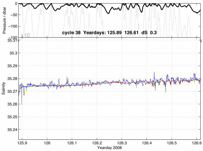
cycle 38 Yeardays: 125.89 126.61 dS 0.3
126.9 127 127.1 127.2 127.3 127.4 127.5 127.6−150
−100
−50
0
x10
Pre
ssur
e / d
bar
126.9 127 127.1 127.2 127.3 127.4 127.5 127.6
35.25
35.26
35.27
35.28
35.29
35.3
35.31
35.32
Sal
inity
Yearday 2008
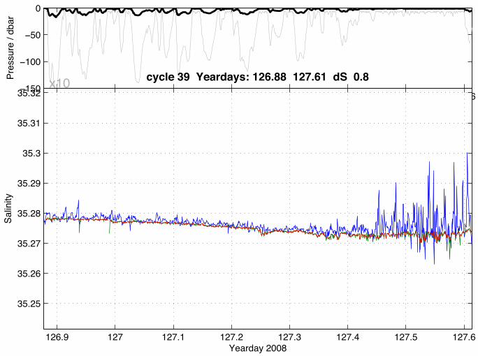
cycle 39 Yeardays: 126.88 127.61 dS 0.8

127.9 128 128.1 128.2 128.3 128.4 128.5 128.6−150
−100
−50
0
x10
Pre
ssur
e / d
bar
127.9 128 128.1 128.2 128.3 128.4 128.5 128.6
35.26
35.27
35.28
35.29
35.3
35.31
35.32
35.33
Sal
inity
Yearday 2008
cycle 40 Yeardays: 127.87 128.61 dS 2.7

128.9 129 129.1 129.2 129.3 129.4 129.5 129.6−150
−100
−50
0
x10
Pre
ssur
e / d
bar
128.9 129 129.1 129.2 129.3 129.4 129.5 129.6
35.25
35.26
35.27
35.28
35.29
35.3
35.31
35.32
Sal
inity
Yearday 2008
cycle 41 Yeardays: 128.88 129.61 dS 4.1

129.9 130 130.1 130.2 130.3 130.4 130.5 130.6−150
−100
−50
0
x10
Pre
ssur
e / d
bar
129.9 130 130.1 130.2 130.3 130.4 130.5 130.6
35.21
35.22
35.23
35.24
35.25
35.26
35.27
35.28
Sal
inity
Yearday 2008
cycle 42 Yeardays: 129.87 130.61 dS 0.2
130.9 131 131.1 131.2 131.3 131.4 131.5 131.6−150
−100
−50
0
x10
Pre
ssur
e / d
bar
130.9 131 131.1 131.2 131.3 131.4 131.5 131.6
35.22
35.23
35.24
35.25
35.26
35.27
35.28
35.29
Sal
inity
Yearday 2008
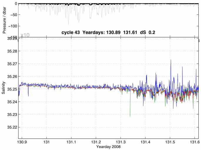
cycle 43 Yeardays: 130.89 131.61 dS 0.2

131.9 132 132.1 132.2 132.3 132.4 132.5 132.6−150
−100
−50
0
x10
Pre
ssur
e / d
bar
131.9 132 132.1 132.2 132.3 132.4 132.5 132.6
35.2
35.21
35.22
35.23
35.24
35.25
35.26
35.27
Sal
inity
Yearday 2008
cycle 44 Yeardays: 131.87 132.61 dS −0.2

133 133.1 133.2 133.3 133.4 133.5 133.6−150
−100
−50
0
x10
Pre
ssur
e / d
bar
133 133.1 133.2 133.3 133.4 133.5 133.6
35.21
35.22
35.23
35.24
35.25
35.26
35.27
35.28
Sal
inity
Yearday 2008
cycle 45 Yeardays: 132.92 133.62 dS −0.4
134 134.1 134.2 134.3 134.4 134.5 134.6−150
−100
−50
0
x10
Pre
ssur
e / d
bar
134 134.1 134.2 134.3 134.4 134.5 134.6
35.21
35.22
35.23
35.24
35.25
35.26
35.27
35.28
Sal
inity
Yearday 2008
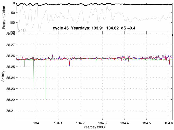
cycle 46 Yeardays: 133.91 134.62 dS −0.4
135 135.1 135.2 135.3 135.4 135.5 135.6−150
−100
−50
0
x10
Pre
ssur
e / d
bar
135 135.1 135.2 135.3 135.4 135.5 135.635.24
35.25
35.26
35.27
35.28
35.29
35.3
35.31
Sal
inity
Yearday 2008
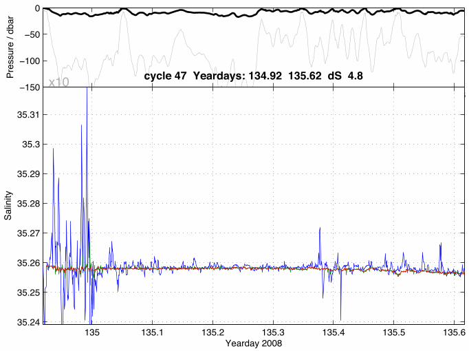
cycle 47 Yeardays: 134.92 135.62 dS 4.8
135.9 136 136.1 136.2 136.3 136.4 136.5 136.6−150
−100
−50
0
x10
Pre
ssur
e / d
bar
135.9 136 136.1 136.2 136.3 136.4 136.5 136.635.21
35.22
35.23
35.24
35.25
35.26
35.27
35.28
Sal
inity
Yearday 2008
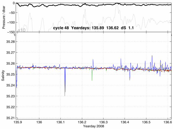
cycle 48 Yeardays: 135.89 136.62 dS 1.1
137 137.1 137.2 137.3 137.4 137.5 137.6−150
−100
−50
0
x10
Pre
ssur
e / d
bar
137 137.1 137.2 137.3 137.4 137.5 137.6
35.23
35.24
35.25
35.26
35.27
35.28
35.29
35.3
Sal
inity
Yearday 2008
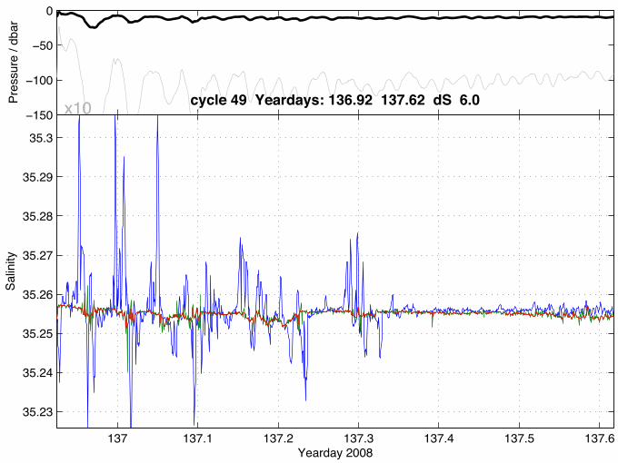
cycle 49 Yeardays: 136.92 137.62 dS 6.0

138 138.1 138.2 138.3 138.4 138.5 138.6−150
−100
−50
0
x10
Pre
ssur
e / d
bar
138 138.1 138.2 138.3 138.4 138.5 138.6
35.21
35.22
35.23
35.24
35.25
35.26
35.27
35.28
Sal
inity
Yearday 2008
cycle 50 Yeardays: 137.94 138.62 dS 0.5

138.9 139 139.1 139.2 139.3 139.4 139.5 139.6−150
−100
−50
0
x10
Pre
ssur
e / d
bar
138.9 139 139.1 139.2 139.3 139.4 139.5 139.6
35.21
35.22
35.23
35.24
35.25
35.26
35.27
35.28
Sal
inity
Yearday 2008
cycle 51 Yeardays: 138.89 139.62 dS 0.7

140 140.1 140.2 140.3 140.4 140.5 140.6−150
−100
−50
0
x10
Pre
ssur
e / d
bar
140 140.1 140.2 140.3 140.4 140.5 140.6
35.2
35.21
35.22
35.23
35.24
35.25
35.26
35.27
Sal
inity
Yearday 2008
cycle 52 Yeardays: 139.91 140.62 dS 0.0

140.8 140.9 141 141.1 141.2 141.3 141.4 141.5 141.6−150
−100
−50
0
x10
Pre
ssur
e / d
bar
140.8 140.9 141 141.1 141.2 141.3 141.4 141.5 141.6
35.17
35.18
35.19
35.2
35.21
35.22
35.23
35.24
Sal
inity
Yearday 2008
cycle 53 Yeardays: 140.75 141.62 dS 0.4

141.9 142 142.1 142.2 142.3 142.4 142.5 142.6−150
−100
−50
0
x10
Pre
ssur
e / d
bar
141.9 142 142.1 142.2 142.3 142.4 142.5 142.6
35.18
35.19
35.2
35.21
35.22
35.23
35.24
35.25
Sal
inity
Yearday 2008
cycle 54 Yeardays: 141.83 142.62 dS 3.6
142.8 142.9 143 143.1 143.2 143.3 143.4 143.5 143.6−150
−100
−50
0
x10
Pre
ssur
e / d
bar
142.8 142.9 143 143.1 143.2 143.3 143.4 143.5 143.6
35.18
35.19
35.2
35.21
35.22
35.23
35.24
35.25
Sal
inity
Yearday 2008
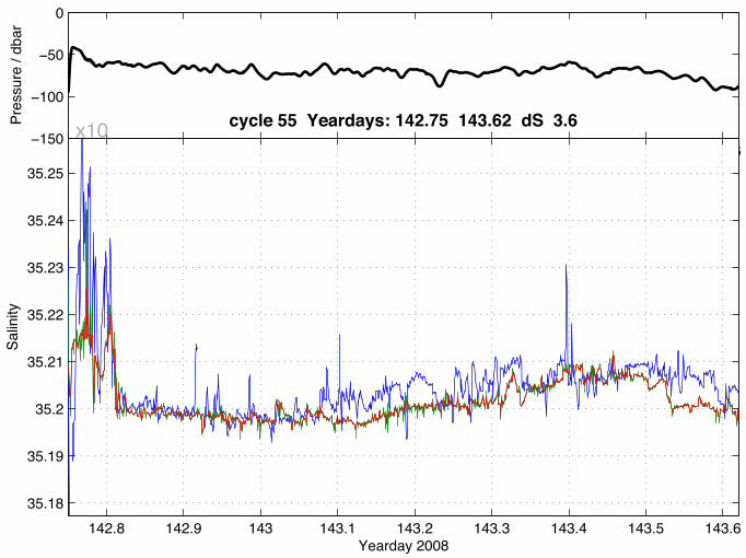
cycle 55 Yeardays: 142.75 143.62 dS 3.6

144 144.1 144.2 144.3 144.4 144.5 144.6−150
−100
−50
0
x10
Pre
ssur
e / d
bar
144 144.1 144.2 144.3 144.4 144.5 144.6
35.2
35.21
35.22
35.23
35.24
35.25
35.26
35.27
Sal
inity
Yearday 2008
cycle 56 Yeardays: 143.91 144.66 dS 0.8
145 145.1 145.2 145.3 145.4 145.5 145.6−150
−100
−50
0
x10
Pre
ssur
e / d
bar
145 145.1 145.2 145.3 145.4 145.5 145.6
35.2
35.21
35.22
35.23
35.24
35.25
35.26
35.27
Sal
inity
Yearday 2008
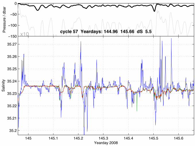
cycle 57 Yeardays: 144.96 145.66 dS 5.5

145.95 146 146.05 146.1 146.15 146.2 146.25 146.3−150
−100
−50
0
x10
Pre
ssur
e / d
bar
145.95 146 146.05 146.1 146.15 146.2 146.25 146.3
35.22
35.23
35.24
35.25
35.26
35.27
35.28
35.29
Sal
inity
Yearday 2008
cycle 58 Yeardays: 145.94 146.31 dS 6.1