summary of the aquavit water vapor intercomparison: 2 ... · 1 summary of the aquavit water vapor...
TRANSCRIPT

23 October 2009 Final Version
1
Summary of the AquaVIT Water Vapor Intercomparison: 1
Static Experiments 2
3
by 4
5
AquaVIT Referees: 6
7
D. W. Fahey, R. S. Gao, 8
Earth System Research Laboratory 9
National Oceanic and Atmospheric Administration 10
Boulder, CO 80305 11
USA 12
13
O. Möhler 14
Forschungszentrum Karlsruhe 15
Institute for Meteorology and Climate Research 16
Atmospheric Aerosol Research (IMK-AAF) 17
76021 Karlsruhe 18
Germany 19
20
22
24
AIDA Facility, Karlsruhe, Germany

23 October 2009 Final Version
2
Table of Contents 1
I. Introduction 2
II. AIDA chamber 3
III. Data Protocol 4
IV. Instruments 5
A. Intercomparison instruments. 6
B. Absolute reference instrument. 7
V. AIDA Chamber Instrument Configuration 8
VI. AquaVIT Static Experiments 9
A. AIDA chamber conditions. 10
B. Static experiment data processing. 11
C. Summary of static experiments: Core instruments. 12
C.1. Reference comparisons. 13
C.2. Uncertainties. 14
C.3. Precision. 15
C.4. Correlations. 16
D. Summary of static experiments: Non-Core instruments. 17
E. Absolute reference instruments 18
VII. Atmospheric Implications of the AquaVIT Static Experiment Results 19
VIII. The AquaVIT Static Experiments: Summary and Conclusions 20
IX. Acknowledgements 21
X. References 22
23
Tables 24
Table 1. Table of AquaVIT intercomparison experiments. 25
Table 2. AquaVIT instruments, participants, and institutes. 26
Table 3. Core and non-core instrument uncertainties during the AquaVIT static experiments. 27
Table 4. Details of AquaVIT static segments used in the accuracy and precision evaluations. 28
Table 5. Experimental upper limits of instrument precision derived from the AquaVIT 29
intercomparison data for selected segments during the static experiments. 30
31
Figures 32
Figure 1. Profile of water vapor mixing ratios from two core instruments included in the 33
AquaVIT intercomparison, CFH and HWV, and the Microwave Limb Sounder 34
(MLS) onboard the NASA Aura satellite. 35
Figure 2. Configuration of the AquaVIT instruments in the AIDA chamber facility. 36
Figure 3. Example of extractive sampling from the AIDA chamber. 37
Figure 4. Non-extractive sampling instruments inside the AIDA chamber. 38
Figure 5. Conditions in the AIDA chamber during the static experiments. 39
Figure 6. Average AIDA chamber pressures and temperatures as a function of the water-40
vapor average reference value for the static experiment segments. 41
Figure 7. Water-vapor ice saturation mixing ratios over the range of total pressures and 42
temperatures in the AIDA chamber during AquaVIT. 43
Figure 8. Time series of AIDA water vapor mixing ratios. 44
Figure 9. Summary plots of static experiment results for core instruments. 45
Figure 10. Summary plots of static experiment results for the core and non-core instruments. 46

23 October 2009 Final Version
3
Figure 11. Summary statistical plots of static experiment results for the core instruments. 1
Figure 12. Summary statistical plots of static experiment results for the core instruments. 2
Figure 13. Correlation plots for core instruments. 3
4
Appendix A. Core instrument descriptions 5
A1. APicT (TDL) 6
A2. Cryogenic Frostpoint Hygrometer (CFH) 7
A3. Fast In situ Stratospheric Hygrometer (FISH-1 & FISH-2) 8
A4. FLuorescent Advanced Stratospheric Hygrometer for Balloon (FLASH-B1 & FLASH-9
B2) 10
A5. Harvard Water Vapour (HWV) 11
A6. JPL Laser Hygrometer (JLH) 12
13
Appendix B. Non-core instrument descriptions 14
B1. MBW-373LX 15
B2. SnowWhite 16
B3. ISOWAT 17
B4. OJSTER 18
B5. PicoSDLA 19
B6. WaSul-Hydro2 20
B7. AIDA PCI extractive TDL (APeT) 21
B8. Closed-path Laser Hygrometer (CLH) 22
B9. VCSEL Hygrometer 23
B10. Fluorescent Water Vapor Sensor (FWVS) 24
25
Appendix C. Reference instruments 26
C1. PTB Water Permeation Source 27
28
29

23 October 2009 Final Version
4
I. Introduction 1
Water vapor is the most important greenhouse gas in the atmosphere and represents a major 2
feedback to warming and other changes in the climate system (Trenberth et al., 2007). 3
Knowledge of the distribution of water vapor and how it is changing as climate changes is 4
especially important in the upper troposphere and lower stratosphere (UT/LS) where water vapor 5
plays a critical role in determining atmospheric radiative balance, cirrus cloud formation, and 6
photochemistry. Dehydration processes reduce water vapor amounts to part per million by 7
volume (ppm) values in UT air before it enters the LS as part of the large-scale circulation of the 8
atmosphere. The microphysics related to dehydration and cirrus cloud nucleation are not fully 9
understood at present, limiting our ability to accurately model the dehydration process and, 10
hence, our ability to fully describe the interaction of the UT/LS water vapor distribution with 11
climate change. 12
Our understanding of water vapor processes in the UT/LS is limited, in part, by large 13
uncertainties in available water measurements, particularly in the 1 to 10 ppm range typical of 14
this region of the atmosphere. For example, in situ instruments involving both extractive and 15
non-extractive sampling on airborne platforms in the UT/LS have consistently shown significant 16
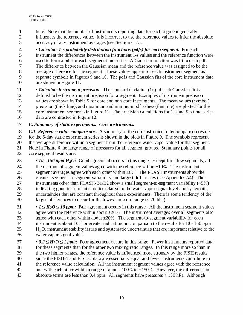
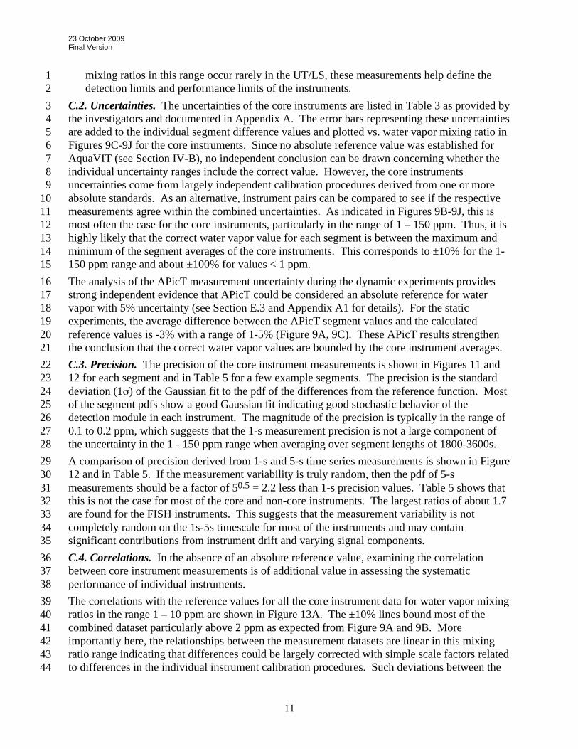
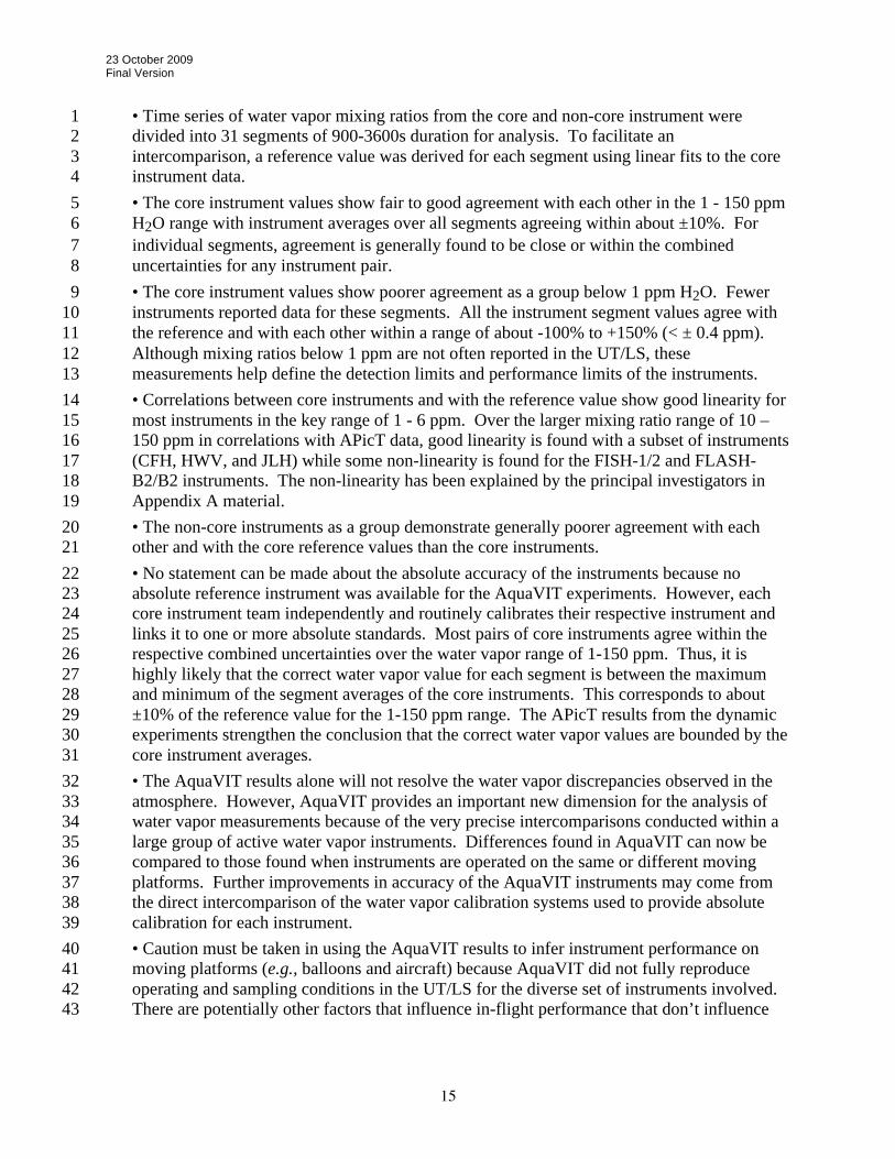
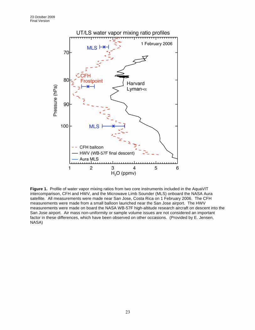
disagreement (up to 50 - 100% or 1-2 ppm) at low water values (< 10 ppm). Examples of 17
tropical profiles with such discrepancies are shown in Figure 1. One important consequence of 18
these differences is that large values of supersaturation over ice have been reported in the UT/LS 19
with the largest being over 100% (Jensen et al., 2005; Peter et al., 2006). At this point in time, 20
such values are unexpected based on our understanding of the fundamental microphysics of ice 21
formation. 22
Discrepancies in water vapor observations have long been noted. The 2000 SPARC Assessment 23
of Upper Tropospheric and Stratospheric Water Vapour (SPARC, 2000) is the most recent 24
comprehensive assessment. It includes intercomparisons of satellite, aircraft, balloon-borne, and 25
ground-based water vapor instrumentation that show discrepancies in the critical range of 1 to 10 26
ppm. Since the SPARC report, discrepancies have remained between key datasets. The 27
AquaVIT campaign was undertaken at the AIDA chamber at Forschungszentrum Karlsruhe as an 28
effort to clarify uncertainties in UT/LS water vapor measurements and help identify the cause(s) 29
of the discrepancies. AquaVIT was designed to reveal instrument calibration and artifact issues 30
that can potentially affect both ground-based and airborne measurements. However, AquaVIT 31
does not address atmospheric sampling issues, which primarily affect in-flight performance, and, 32
thus, require separate evaluation approaches. 33
AquaVIT was a controlled, refereed, blind intercomparison of principal airborne field 34
instruments using the AIDA chamber. Conditions in the chamber ranged over pressure, 35
temperature and water vapor conditions found in the tropical UT/LS. Advantages of the 36
AquaVIT approach are that, by comparing instruments in a controlled ground-based facility, 37
systematic measurement problems and perhaps their causes could be identified more readily and 38
with less expense and effort than in airborne campaigns. In addition, AquaVIT included 39
instruments that were relatively new to atmospheric measurements or still under development in 40
order to accelerate their progress in becoming reliable and accurate water vapor instruments for 41
use in future field measurement campaigns. 42
The AquaVIT experiments occurred in two one-week phases in October 2007 in Karlsruhe, 43
Germany. The first phase was devoted to static intercomparisons with a separate experiment 44

23 October 2009 Final Version
5
each day (15-19 October) at almost constant pressure and temperature conditions. The second 1
phase was a week of dynamic intercomparisons, with several experiments each day (22-26 2
October) under varying pressure, temperature and humidity conditions and with the absence and 3
presence of ice clouds. Instruments participated in one or both phases. A summary of chamber 4
conditions during each intercomparison week is shown in Table 1. In this document, only the 5
static experiments and their results are described. 6
7
II. AIDA chamber 8
The Aerosol Interaction and Dynamics in the Atmosphere (AIDA) chamber is located at 9
Forschungszentrum Karlsruhe. The chamber is an aluminum vessel of volume 84 m3 with 10
facility to control pressure from an atmosphere to as low as 0.01 mbar and temperature from 11
ambient to as low as 182K (Möhler et al., 2003). This range of conditions allows for simulating 12
atmospheric aerosol and cloud processes in the troposphere and lower stratosphere on short 13
(minutes) to long (days) time scales. Important features of the AIDA chamber for AquaVIT 14
were: 15
• Static and dynamic conditions. The operation of the chamber allowed for static conditions 16
of near-constant pressure (±1 hPa), temperature (±0.3 K), and humidity, and for dynamic 17
conditions during which the pressure, temperature and humidity were altered by the addition 18
of dry air or the partial removal of chamber air by pumping. Ice clouds were occasionally 19
formed by the removal of chamber air, which causes adiabatic cooling, or by injection of 20
water. 21
• Large capacity. The large chamber volume allowed multiple instruments outside the 22
chamber to extract sample air for extended periods with only slow changes occurring in the 23
relative humidity or pressure inside the chamber. In addition, several non-extractive 24
sampling instruments were located inside without significantly altering chamber conditions. 25
• Relative humidity range. The relative humidity in the chamber was controlled by direct 26
water addition, wall temperature changes, and controlled evacuation of the chamber to match 27
conditions in the upper troposphere and lower stratosphere (UT/LS), i.e., water vapor mixing 28
ratios < 20 ppm, pressures < 200 hPa, and temperatures between 180K and 210K. 29
• Customized extractive sampling probes. Customized, extractive sampling probes were 30
implemented for AquaVIT to bring chamber air to instruments located outside the chamber. 31
The probes were made of stainless steel and heated to avoid water adsorption on the probe 32
inner walls at low chamber temperatures. 33
34
III. Data Protocol 35
All investigators signed the data protocol adopted for AquaVIT. The protocol encouraged rapid 36
assessment and use of the results from the AquaVIT tests while upholding the rights of the 37
individual scientists and treating all participants equitably. Key features of the protocol are: 38
• Quick-look data. Preliminary or quick-look data obtained during the AquaVIT campaign 39
were made available to the referees as soon as possible following each day’s experiments 40
(< 24 hrs). In the event of obvious difficulties, this allowed the referees to suggest 41
corrections or amendments to data processing, instrument configuration, or instrument 42
operation be made as soon as possible, thereby improving the overall outcome of the 43

23 October 2009 Final Version
6
intercomparison; 1
• Blind intercomparison. A blind intercomparison was established so that preliminary data 2
submitted during the campaign and the short evaluation period immediately following the 3
campaign were available outside the investigator groups only to the referees (O. Möhler, 4
D. W. Fahey, and R. S. Gao); 5
• Final data. After the end of the short evaluation period (4 December 2007) the submitted 6
datasets were released to all participants. Any further changes to a submitted dataset 7
required documentation from an instrument’s Principal Investigator and approval by the 8
referees. All datasets were considered final on 10 January 2008. 9
A dedicated wikipage with password protection enabled archiving and interchange of datasets 10
among the participants and access to other AquaVIT documents and information. 11
(https://aquavit.icg.kfa-juelich.de/AquaVit/) 12
13
IV. Instruments 14
A. Intercomparison instruments. AquaVIT included 25 different instruments utilizing both 15
state-of-the-art and newly developed techniques (Table 2). The instruments were provided and 16
managed by 17 investigator groups from 7 countries, thereby representing a large fraction of the 17
upper-atmosphere water-vapor community. Four categories of AquaVIT instruments are listed 18
in Table 2 and described in the following sections. 19
• Core instruments. The core instrument group for the intercomparison is comprised of eight 20
water vapor instruments: APicT, CFH, FISH-1, FISH-2, FLASH-B1, FLASH-B2, HWV, 21
JLH. The APicT, as an AIDA facility instrument, has been involved in many AIDA chamber 22
experiments. The other instruments have a long history of field measurements and 23
intercomparisons on balloon and aircraft platforms operating in the upper troposphere and 24
stratosphere. The mixing ratio discrepancies noted at low values in these regions derive from 25
a variety of datasets from these instruments. Establishing the accuracy of the core 26
instruments under controlled laboratory conditions was the primary objective of AquaVIT. 27
The accuracy and precision for each of the core instruments are listed in Table 3 as provided 28
by the Principal Investigators. 29
• Formal intercomparison instruments. Ten non-core instruments participated formally in 30
the blind, refereed intercomparison. The group included mature instruments that had been 31
used in field measurements as well as instruments that were in the initial to later stages of 32
development. For three of these instruments (APeT, DM500, and VCSEL) no statistical 33
analyses were performed for the static experiments due to the submission of no data or 34
insufficient data. 35
• Informal intercomparison instruments. Four non-core instruments did not participate in 36
the blind, refereed intercomparison because of instrument or configuration difficulties during 37
the campaign that limited the collection of science-quality data. 38
• Instruments with no participation. Three non-core instruments did not participate in the 39
data intercomparison because instrument or configuration difficulties were sufficiently severe 40
that no science-quality data could be submitted. 41
Brief descriptions of the core (non-core) instruments, their configuration in the AIDA chamber, 42
their performance during the static experiments and lessons learned from AquaVIT are included 43

23 October 2009 Final Version
7
in Appendix A (B). The AIDA configurations for most instruments were not identical to their 1
operation in the field on moving platforms, thereby creating concerns related, for example, to 2
sample flow, contamination, or background signals. The interpretation of the AquaVIT results 3
presented here must take these concerns into account before the results can be used to evaluate 4
the discrepancies in the field observations. 5
B. Reference instruments. There was no water vapor instrument designated as the absolute 6
reference for the AquaVIT intercomparison. An absolute reference instrument would provide 7
reliable and consistent measurements of the chamber water-vapor mixing ratio, either with 8
extractive or non-extractive sampling, over a large range of pressure, temperature, and humidity 9
conditions with objective uncertainty estimates and calibration traceable to international 10
calibration standards. No AquaVIT instrument has been shown to meet those criteria. However, 11
the analysis of the APict data from the dynamic experiments provides strong evidence that APict 12
could serve as an absolute reference instrument for the static intercomparisons. In addition, the 13
MBW-373LX frostpoint and a calibrated permeation source for water vapor were also used as 14
reference instruments in separate intercomparisons with individual instruments. These reference 15
instruments are discussed in Section E. In the absence of an absolute reference instrument for 16
AquaVIT, the reference values used in the intercomparison analyses were derived from the core 17
instrument values as described in Section VI.B. 18
19
V. AIDA Chamber Instrument Configuration 20
The overall configuration of AquaVIT instruments in the AIDA chamber facility is shown in 21
Figure 2. The instrument sampling techniques can be classified into two distinct types. The first 22
type is extractive sampling, which requires gas be removed through a heated probe located inside 23
the chamber and through heated sample lines that pass through the chamber and thermal 24
enclosure walls. Of the core instruments, CFH, FISH-1, FISH-2, FLASH-B2, and HWV used 25
extractive sampling. Of all the instruments with extractive sampling, three were located outside 26
the chamber but inside the chamber thermal enclosure (OJSTER, PicoSDLA, and NCAR-Buck). 27
Chamber sampling probes and the HWV configuration are shown in Figure 3. 28
The second type is internal or non-extractive sampling. Three core instruments (APicT, FLASH-29
B1, and JLH) and one non-core instrument (SnowWhite) used non-extractive sampling. APict 30
and JLH used open-path optical absorption spectroscopy and FLASH-B1 used fluorescence to 31
measure water vapor directly inside the chamber without extracting or modifying the gas volume 32
in the measurement area. The JLH laser, detector, and optical path (with a virtual sampling 33
volume of approximately 1.6 liters) were mounted entirely inside the chamber, as was the 34
SnowWhite instrument sensor (Figure 4). For both of these instruments, the associated control 35
and data recording electronics remained outside the thermal enclosure. The APicT and FLASH-36
B1 instruments also probed chamber air without extractive sampling by having optical paths 37
located inside the chamber, and instrument locations outside the chamber but inside the thermal 38
enclosure (except for some electronic components). The APicT was the only instrument that 39
provided a measurement of the average water-vapor abundance over the full diameter of the 40
chamber by folding its optical path between the inner chamber walls. Some part of the APicT 41
optics (and 0.5% of the total absorption path) was located outside the main chamber but in the 42
cold, dry area inside the thermal enclosure. The FLASH-B1 instrument was mounted outside the 43
chamber wall and measured water vapor optically through an opening in the wall. 44

23 October 2009 Final Version
8
A flow of chamber air was required for all of the extractive instruments with nominal values 1
indicated in Figure 2. The flow was maintained with pumps provided by the investigators or the 2
large auxiliary pumping system available in the AIDA facility. The maintenance of mass flow 3
rates sufficiently large to adequately simulate instrument operation in field sampling was a 4
concern for some instruments, especially at the lowest chamber pressures. 5
6
VI. AquaVIT Static Experiments 7
A. AIDA chamber conditions. The static intercomparison experiments were characterized by 8
• Constant chamber temperature. The temperature was reduced in daily steps from ~240K 9
on the first day to ~185K on the last day. The temperature was stable to ±0.3K during the 10
measurement segments. 11
• Constant chamber pressure. The pressure was held constant in 0.5 - 1-hr intervals or 12
segments (approximately 7) during each day. The pressure in consecutive intervals started at 13
~50 hPa, increased to 300 or 500 hPa and then decreased to ~50hPa. The pressure was stable 14
to ±1 hPa during the measurement segments. 15
• Controlled range of water-vapor mixing ratio values. The mixing ratio varied depending 16
on the amount of water added directly to the chamber at the beginning of each day’s 17
experiment and on the subsequent changes in chamber conditions. 18
The actual pressure and temperature time series for the static experiments are shown in Figure 5. 19
The transient temperature excursions in the time series are the adiabatic responses to the 20
occasional rapid addition or removal of air from the chamber. 21
The static intercomparisons were divided into intervals or segments of constant pressures and 22
temperatures. Figure 6 and Table 4 show the average pressure, temperature, and water-vapor 23
mixing ratio values for the segments used in the accuracy and precision analyses presented 24
below. During each segment, the pressure slowly decreased due to the extractive sampling of 25
chamber air by many of the instruments. From the flow values in Figure 2, the total extractive 26
flow was typically in the range 50 – 140 standard l/min depending on the exact instrument 27
configuration and operating conditions. This range corresponds to a removal of 0.05 – 0.16% of 28
the total chamber volume (84 m3) each minute. As the pressure decreased in the chamber, a 29
servo control system added dry air (< 3 ppm) to maintain pressure constant within ±1 hPa. 30
During the static segments with constant pressure, the gas temperatures measured at various 31
chamber locations deviated by less than 0.3 K from the average AIDA air temperature. A large 32
vane-axial fan inside the chamber was used routinely to promote uniform mixing ratio and 33
temperature conditions throughout the chamber (Möhler et al., 2003). 34
Overnight between experiments the chamber was fully evacuated (< 0.01 hPa). Each morning, 35
an amount of pure water vapor was added to the chamber and then subsequently diluted during 36
the first half of the day as dry air (< 3 ppm) was added to the chamber to increase the total 37
pressure stepwise to 500 hPa. The amount of water vapor was kept below ice saturation values 38
(Figure 7). The resulting water vapor mixing ratios in the static measurement segments varied 39
from 0.2 to 150 ppm as shown in Table 4. 40
Under certain situations the gas-phase water-vapor mixing ratio is not conserved in the AIDA 41
chamber. The first situation occurs when the water vapor mixing ratio of the synthetic air added 42
for constant pressure regulation during sampling periods or for increasing the chamber total 43

23 October 2009 Final Version
9
pressure differs from the water vapor mixing ratio present in the chamber air. Generally the 1
added air is drier than the chamber air causing the mixing ratio to decrease with time. The 2
second situation occurs when the chamber walls are at least partially coated with ice. Wall ice 3
acts as a source or sink of water vapor in the chamber, depending on the actual partial pressure in 4
the chamber volume and the saturation pressure above the wall ice coating. The effects of this 5
source are clearly demonstrated by water vapor mixing ratios that do not remain constant when 6
the chamber pressure is decreased by pumping with wall-ice present. Non-conservation was also 7
observed to a lesser extent in the ice-free static experiments due to the adsorption and desorption 8
of water on the walls. Examples of this are shown by the time series in Figure 8 in which the 9
water vapor mixing ratio increases when the chamber pressure is reduced in the second half of 10
the day’s experiment. If there are no other sources of water vapor then the mixing ratio should 11
remain constant as air is pumped from the chamber. Non-conservation of water vapor does not 12
interfere fundamentally with the AquaVIT results because the water vapor mixing ratios always 13
changed slowly with time within an intercomparison segment and remained uniform inside the 14
chamber with stirring from an internal fan (see discussion below). 15
B. Static experiment data processing. For each day of the static experiment series, the 16
instrument teams submitted a data file reporting water vapor mixing ratios vs. UT time. The 17
measurement interval for most instruments was 1 s. As an example, the 1-s datasets for 15 18
October are plotted in Figure 8 on logarithmic and linear scales. The maximum differences in 19
absolute value and variability are large, particularly at low mixing ratios. 20
The data processing steps taken for the combined dataset were the following: 21
• Define segments. The time series were divided into constant pressure and near constant 22
temperature segments for statistical analysis. Not all segments were used in the 23
intercomparison analysis. The criteria for selecting a segment were near-constant or slowly 24
and linearly varying water vapor mixing ratios within the segment and the availability of 25
water vapor data for the segment from a majority of the core instruments. The first criterion 26
ensured uniform mixing ratio conditions in the chamber and, hence, each sample line. In 27
defining the segments, measurements during addition or removal of chamber air were 28
excluded because the chamber conditions were rapidly changing and generally less uniform. 29
Constant or linearly varying water vapor values in a segment were also key to the precision 30
analysis described below. Segment lengths in the range 900-3600s were chosen to provide 31
good statistical confidence in the subsequent analysis steps. The times and lengths of the 32
segments used in the analysis along with average pressure, temperature, and water-vapor 33
mixing ratios are provided in Table 4. 34
• Calculate linear fits for each instrument segment. A linear fit was performed on the time 35
series data for each core instrument for each segment. 36
• Calculate reference water vapor mixing ratios. The reference water-vapor mixing ratio 37
for each segment was obtained using only the core instrument data. A two-step process was 38
adopted to provide a consistent basis of comparison across and within segments. First, a 39
single linear fit was performed on the complete set of core linear fits. This combined fit was 40
chosen over a simple average of all core instrument data in order to give the same weight to 41
all core instruments in deriving the reference value. This combined fit is defined as the 42
reference function for the segment. Second, the reference water-vapor mixing ratio for the 43
segment was defined to be the average of the reference function over the segment. These 44
reference values as listed in Table 4 are used throughout the analysis and plots presented 45
23 October 2009 Final Version
10
here. Note that the number of instruments reporting data for each segment generally 1
influences the reference value. It is incorrect to use the reference values to infer the absolute 2
accuracy of any instrument averages (see Section C.2.). 3
• Calculate 1-s probability distribution functions (pdfs) for each segment. For each 4
instrument the differences between the instrument 1-s values and the reference function were 5
used to form a pdf for each segment time series. A Gaussian function was fit to each pdf. 6
The difference between the Gaussian mean and the reference value was assigned to be the 7
average difference for the segment. These values appear for each instrument segment as 8
separate symbols in Figures 9 and 10. The pdfs and Gaussian fits of the core instrument data 9
are shown in Figure 11. 10
• Calculate instrument precision. The standard deviation (1 ) of each Gaussian fit is 11
defined to be the instrument precision for a segment. Examples of instrument precision 12
values are shown in Table 5 for core and non-core instruments. The mean values (symbol), 13
precision (thick line), and maximum and minimum pdf values (thin line) are plotted for the 14
core instrument segments in Figure 11. The precision calculations for 1-s and 5-s time series 15
data are contrasted in Figure 12. 16
C. Summary of static experiments: Core instruments. 17
C.1. Reference value comparisons. A summary of the core instrument intercomparison results 18
for the 5-day static experiment series is shown in the plots in Figure 9. The symbols represent 19
the average difference within a segment from the reference water vapor value for that segment. 20
Note in Figure 6 the large range of pressures for all segment groups. Summary points for all 21
core segment results are: 22
• 10 - 150 ppm H2O: Good agreement occurs in this range. Except for a few segments, all 23
the instrument segment values agree with the reference within ±10%. The instrument 24
segment averages agree with each other within ±6%. The FLASH instruments show the 25
greatest segment-to-segment variability and largest differences (see Appendix A4). The 26
instruments other than FLASH-B1/B2 show a small segment-to-segment variability (~5%) 27
indicating good instrument stability relative to the water vapor signal level and systematic 28
uncertainties that are constant throughout these experiments. There is some tendency of the 29
largest differences to occur for the lowest pressure range (< 70 hPa). 30
• 1 H2O 10 ppm: Fair agreement occurs in this range. All the instrument segment values 31
agree with the reference within about ±20%. The instrument averages over all segments also 32
agree with each other within about ±20%. The segment-to-segment variability for each 33
instrument is about 10% or greater indicating, in comparison to the results for 10 - 150 ppm 34
H2O, instrument stability issues and systematic uncertainties that are important relative to the 35
water vapor signal value. 36
• 0.2 H2O 1 ppm: Poor agreement occurs in this range. Fewer instruments reported data 37
for these segments than for the other two mixing ratio ranges. In this range more so than in 38
the two higher ranges, the reference value is influenced more strongly by the FISH results 39
since the FISH-1 and FISH-2 data are essentially equal and fewer instruments contribute to 40
the reference value calculation. All the instrument segment values agree with the reference 41
and with each other within a range of about -100% to +150%. However, the differences in 42
absolute terms are less than 0.4 ppm. All segments have pressures > 150 hPa. Although 43
23 October 2009 Final Version
11
mixing ratios in this range occur rarely in the UT/LS, these measurements help define the 1
detection limits and performance limits of the instruments. 2
C.2. Uncertainties. The uncertainties of the core instruments are listed in Table 3 as provided by 3
the investigators and documented in Appendix A. The error bars representing these uncertainties 4
are added to the individual segment difference values and plotted vs. water vapor mixing ratio in 5
Figures 9C-9J for the core instruments. Since no absolute reference value was established for 6
AquaVIT (see Section IV-B), no independent conclusion can be drawn concerning whether the 7
individual uncertainty ranges include the correct value. However, the core instruments 8
uncertainties come from largely independent calibration procedures derived from one or more 9
absolute standards. As an alternative, instrument pairs can be compared to see if the respective 10
measurements agree within the combined uncertainties. As indicated in Figures 9B-9J, this is 11
most often the case for the core instruments, particularly in the range of 1 – 150 ppm. Thus, it is 12
highly likely that the correct water vapor value for each segment is between the maximum and 13
minimum of the segment averages of the core instruments. This corresponds to ±10% for the 1-14
150 ppm range and about ±100% for values < 1 ppm. 15
The analysis of the APicT measurement uncertainty during the dynamic experiments provides 16
strong independent evidence that APicT could be considered an absolute reference for water 17
vapor with 5% uncertainty (see Section E.3 and Appendix A1 for details). For the static 18
experiments, the average difference between the APicT segment values and the calculated 19
reference values is -3% with a range of 1-5% (Figure 9A, 9C). These APicT results strengthen 20
the conclusion that the correct water vapor values are bounded by the core instrument averages. 21
C.3. Precision. The precision of the core instrument measurements is shown in Figures 11 and 22
12 for each segment and in Table 5 for a few example segments. The precision is the standard 23
deviation (1 ) of the Gaussian fit to the pdf of the differences from the reference function. Most 24
of the segment pdfs show a good Gaussian fit indicating good stochastic behavior of the 25
detection module in each instrument. The magnitude of the precision is typically in the range of 26
0.1 to 0.2 ppm, which suggests that the 1-s measurement precision is not a large component of 27
the uncertainty in the 1 - 150 ppm range when averaging over segment lengths of 1800-3600s. 28
A comparison of precision derived from 1-s and 5-s time series measurements is shown in Figure 29
12 and in Table 5. If the measurement variability is truly random, then the pdf of 5-s 30
measurements should be a factor of 50.5 = 2.2 less than 1-s precision values. Table 5 shows that 31
this is not the case for most of the core and non-core instruments. The largest ratios of about 1.7 32
are found for the FISH instruments. This suggests that the measurement variability is not 33
completely random on the 1s-5s timescale for most of the instruments and may contain 34
significant contributions from instrument drift and varying signal components. 35
C.4. Correlations. In the absence of an absolute reference value, examining the correlation 36
between core instrument measurements is of additional value in assessing the systematic 37
performance of individual instruments. 38
The correlations with the reference values for all the core instrument data for water vapor mixing 39
ratios in the range 1 – 10 ppm are shown in Figure 13A. The ±10% lines bound most of the 40
combined dataset particularly above 2 ppm as expected from Figure 9A and 9B. More 41
importantly here, the relationships between the measurement datasets are linear in this mixing 42
ratio range indicating that differences could be largely corrected with simple scale factors related 43
to differences in the individual instrument calibration procedures. Such deviations between the 44

23 October 2009 Final Version
12
instruments might be removed by the introduction of a unified, traceable calibration procedure 1
for all instruments using the same high-accuracy water vapor source. Exceptions to simple scale 2
factors are the clusters of HWV and FISH-1/2 data points near 2 ppm that are offset from the 3
linear correlation of the remaining data. 4
The correlations with APicT data over the full mixing ratio range are shown in Figure 13 for all 5
other core instruments. APicT was chosen as the common dataset in each plot instead of the 6
reference values because APicT reported data for all segments and APicT average values are 7
uniformly close to the reference values over the range 1-150 ppm. Three instruments (CFH, 8
HWV, and JLH) show a linear relation to APicT (and, hence, to each other) over the entire 9
range. This indicates that differences between these datasets could be removed with scale 10
factors. The remaining instruments (FISH-1/2 and FLASH-B2) show a much less linear 11
correlation over the mixing ratio range. For FISH-1 and FISH-2, the correlation slope changes 12
significantly above about 100 ppm. For FLASH-B1 and FLASH-B2, there are irregularities in 13
the slope below about 50 ppm. For FLASH-B2, the correlation slope changes gradually with 14
increasing mixing ratio above 50 ppm. The slope changes for the FISH and FLASH instruments 15
have been explained by the principal investigators (see Appendix A). 16
D. Summary of static experiments: Non-Core instruments. 17
A summary of the formal intercomparison results for the non-core instruments is shown in 18
Figure 10 for the 5-day static experiment series. Plot details are the same as described above for 19
Figure 9. The segment reference functions and values for the non-core instruments are those 20
derived for the core instrument intercomparisons. Figure 10A shows a combination of results 21
from the seven non-core instruments and the eight core instruments. Missing in Figure 10A are 22
data for VCSEL and APeT, which submitted data only for the dynamic experiments, and for 23
DM500, which submitted data insufficient for the statistical analysis presented here. 24
Summary points for all non-core segment results are: 25
• 10 - 150 ppm H2O: The best overall agreement with the core reference values occurs in 26
this range. Segment differences show a wider range than core instruments, varying from 27
about -100% to +200% with most of the data falling within the -30% to +50% range. 28
Instrument averages also show a wider range, varying from about -90% to +40%. 29
• 1 H2O 10 ppm: Poorer agreement with the core reference values occurs in this range. 30
Segment differences show a much wider range than core instruments, varying from about -31
20% to +1000% with most instruments significantly higher than the reference value. 32
• 0.2 H2O 1 ppm: The poorest agreement with the core reference values occurs in this 33
range as also found for the core instruments. Only two instruments submitted data for these 34
low values. The results are 100-300% higher than the reference value. 35
A comparison of core/non-core instrument results in Figure 10A reveals that far fewer segment 36
values are available from the non-core instruments. Notable exceptions are the PicoSDLA and 37
Wasul-Hygro2 instruments, which reported data for each segment. However, only a few 38
segments could be analyzed for Wasul-Hygro2 due to its low data-sampling rate. 39
E. Absolute reference instruments. 40
Three AquaVIT instruments have relevance in serving as absolute reference standards. The 41
MBW-373LX and the PTB water vapor permeation source have direct links to international 42

23 October 2009 Final Version
13
standards. APicT was tested during AquaVIT under ice-saturation conditions, which allows a 1
direct comparison to laboratory ice-saturation equilibrium vapor pressures. 2
E.1. MBW-373LX. The AIDA facility regularly uses a chilled-mirror frostpoint hygrometer 3
from MBW Calibration Ltd. in Switzerland (MBW-373LX, see http://www.mbw.ch). The 4
MBW unit has a frost point accuracy of ±0.1K traceable to calibration standards maintained by 5
the German metrology laboratory (Physikalisch-Technische Bundesanstalt (PTB)) and linked to 6
international standards. The MBW-373LX unfortunately is not designed to operate with sample 7
line pressures less than one atmosphere and thus could not be used as the reference instrument in 8
AquaVIT. Near atmospheric pressure, however, the MBW hygrometer has intercompared well 9
with the APicT, another facility instrument, in many previous AIDA experiments. 10
E.2. PTB water vapor permeation source. A calibrated permeation source of water vapor was 11
provided to the AquaVIT team during the experiment period by Dr. Peter Mackrodt of PTB in 12
Germany. The calibration accuracy is 2% for mixing ratios between 0.5 and 5 ppm. Three 13
instruments, CFH, MBW-373LX, and VCSEL were intercompared to the device, which provided 14
a small gas flow with a known mixing ratio of water vapor. Details of the permeation source and 15
some intercomparison results are described in Appendix C. Reported differences were <±10%. 16
E.3. APicT. The APicT water vapor mixing rations were compared to equilibrium ice saturation 17
values during the AquaVIT dynamic experiments. During the experiments, dense ice clouds 18
were present in the AIDA chamber under almost constant pressure and temperature conditions. 19
As a consequence, the water vapor mixing ratios inside the chamber were assumed to be ice-20
saturation values at the respective gas temperatures. The variability of the gas temperatures 21
measured throughout the chamber volume was typically less than ±0.2 °C, which means that the 22
variability of the water saturation pressure above the ice-crystal phase was less than about ±3%. 23
The average values of water vapor and temperature in the ice-saturated segments varied over 24
wide ranges (0.01-40 Pa and 185-243K) (Table 1, Figure A1.1). During the segments, the water-25
vapor partial pressure measured in situ with the APicT instrument deviated by less than ±3% 26
from the ice-saturation pressures calculated from laboratory vapor pressure relations, which have 27
an estimated uncertainty of ±1% (Murphy and Koop, 2005) (Figure A1.1). Within estimated 28
uncertainty limits of about 5%, APicT values agreed with the expected ice-saturation values. 29
30
VII. Atmospheric Implications of the AquaVIT Static Experiment Results 31
The AquaVIT results have implications for atmospheric measurements of water vapor made by 32
the AquaVIT core instruments in the UT/LS region. The mixing ratio values in AquaVIT 33
spanned the range of <1 - 150 ppm, which is highly relevant for the tropical UT/LS where 34
dehydration processes produce the lowest mixing ratios generally observed in the atmosphere. 35
The core instrument results showed agreement in the key 1-10 ppm range within about ±10%. 36
Part of the motivation for AquaVIT was to provide a partial basis to resolve the field 37
discrepancies observed when core instruments are operated in the UT/LS on the same or 38
different moving platforms (Vömel, 2006; Peter et al., 2006). In some cases, these discrepancies 39
are large enough (50 - 100%) to interfere with answering important scientific questions about 40
water vapor in the UT/LS. An example of differences associated with core instruments is shown 41
in Figure 1. An important conclusion from AquaVIT is that the differences observed in the field 42
(Figure 1) are significantly larger than those found for CFH and HWV in the static experiments 43
as shown in Figure 9. However, the qualitative differences are similar, with CFH values less 44
than HWV values. Further conclusions may follow from a systematic assessment of the field 45

23 October 2009 Final Version
14
observations by instrument investigators that includes the AquaVIT results. Instrument response 1
to changing water vapor abundances will be investigated further using data from the Aquavit 2
dynamic experiments and presented in a separate white paper. 3
Caution must be taken in using the static intercomparison results to infer instrument performance 4
on moving platforms (e.g., balloons and aircraft) because AquaVIT did not fully reproduce 5
UT/LS instrument or sampling conditions for the diverse set of instruments involved, nor could it 6
be expected to. For example, the extractive sampling instruments in AquaVIT were not under 7
the same physical conditions that they experience on moving platforms in the UT/LS. For those 8
instruments mounted outside the AIDA chamber, ambient pressures and/or temperatures were 9
generally significantly higher than typically encountered in UT/LS flights. Similarly, sample 10
flows (i.e., internal to the instruments) were also at higher temperatures. In the AquaVIT 11
configuration, a closer simulation of external and internal pressures and temperatures occurred 12
for JLH and SnowWhite because both were located inside the chamber. However, sample-13
volume flow rates were not well simulated. Of specific concern for the AquaVIT configuration 14
are sample air temperatures that were near room temperature (~300K) instead of typical UT/LS 15
values (< 220K) for instruments with extractive sampling, and sample flows that were lower than 16
under flight conditions, for example, in the case of HWV. There are potentially other factors that 17
influence in-flight performance in the UT/LS that don’t influence the AquaVIT experiments, 18
such as rapid changes in mixing ratio. These effects will need to be carefully evaluated to make 19
appropriate and optimal use of the AquaVIT results presented here. 20
As discussed in the Introduction, SPARC published systematic analyses and intercomparisons of 21
the field observations involving key water vapor instruments (SPARC, 2000). An update to the 22
SPARC water vapor assessment is now being planned. The AquaVIT results will offer a new 23
dimension of analysis for this updated assessment and may help resolve some of the 24
longstanding discrepancies in field observations. In addition, the AquaVIT results and 25
experimental process form a basis to plan follow-on laboratory evaluations of current and new 26
water vapor instrumentation. 27
28
VIII. Summary of the AquaVIT Static Experiments 29
The static experiment results are summarized as follows: 30
• The AquaVIT experiment successfully integrated 25 instruments to measure water vapor in 31
the AIDA chamber using either extractive or non-extractive sampling methods. The 32
scientific and technical participant group developed procedures and protocols to carry out the 33
physical experiments and post-experiment data processing and analysis. For five days in 34
October 2007, static experiments were conducted with chamber conditions covering a range 35
of pressures (50-500 hPa), temperatures (185-243K) and water vapor mixing ratios (<1-150 36
ppm) in order to simulate conditions typically found in the UT/LS. 37
• A majority of AquaVIT instruments reported a full or partial dataset for the 5 days of static 38
experiments. The reporting instruments were divided into two categories: core and non-core 39
instruments. Core instruments have been extensively used in field campaigns on moving 40
platforms and are as a group associated with the large systematic discrepancies that have 41
been observed in the UT/LS, particularly in the tropics. Several of the non-core instruments 42
are newly developed and undergoing intercomparison for the first time. 43
23 October 2009 Final Version
15
• Time series of water vapor mixing ratios from the core and non-core instrument were 1
divided into 31 segments of 900-3600s duration for analysis. To facilitate an 2
intercomparison, a reference value was derived for each segment using linear fits to the core 3
instrument data. 4
• The core instrument values show fair to good agreement with each other in the 1 - 150 ppm 5
H2O range with instrument averages over all segments agreeing within about ±10%. For 6
individual segments, agreement is generally found to be close or within the combined 7
uncertainties for any instrument pair. 8
• The core instrument values show poorer agreement as a group below 1 ppm H2O. Fewer 9
instruments reported data for these segments. All the instrument segment values agree with 10
the reference and with each other within a range of about -100% to +150% (< ± 0.4 ppm). 11
Although mixing ratios below 1 ppm are not often reported in the UT/LS, these 12
measurements help define the detection limits and performance limits of the instruments. 13
• Correlations between core instruments and with the reference value show good linearity for 14
most instruments in the key range of 1 - 6 ppm. Over the larger mixing ratio range of 10 – 15
150 ppm in correlations with APicT data, good linearity is found with a subset of instruments 16
(CFH, HWV, and JLH) while some non-linearity is found for the FISH-1/2 and FLASH-17
B2/B2 instruments. The non-linearity has been explained by the principal investigators in 18
Appendix A material. 19
• The non-core instruments as a group demonstrate generally poorer agreement with each 20
other and with the core reference values than the core instruments. 21
• No statement can be made about the absolute accuracy of the instruments because no 22
absolute reference instrument was available for the AquaVIT experiments. However, each 23
core instrument team independently and routinely calibrates their respective instrument and 24
links it to one or more absolute standards. Most pairs of core instruments agree within the 25
respective combined uncertainties over the water vapor range of 1-150 ppm. Thus, it is 26
highly likely that the correct water vapor value for each segment is between the maximum 27
and minimum of the segment averages of the core instruments. This corresponds to about 28
±10% of the reference value for the 1-150 ppm range. The APicT results from the dynamic 29
experiments strengthen the conclusion that the correct water vapor values are bounded by the 30
core instrument averages. 31
• The AquaVIT results alone will not resolve the water vapor discrepancies observed in the 32
atmosphere. However, AquaVIT provides an important new dimension for the analysis of 33
water vapor measurements because of the very precise intercomparisons conducted within a 34
large group of active water vapor instruments. Differences found in AquaVIT can now be 35
compared to those found when instruments are operated on the same or different moving 36
platforms. Further improvements in accuracy of the AquaVIT instruments may come from 37
the direct intercomparison of the water vapor calibration systems used to provide absolute 38
calibration for each instrument. 39
• Caution must be taken in using the AquaVIT results to infer instrument performance on 40
moving platforms (e.g., balloons and aircraft) because AquaVIT did not fully reproduce 41
operating and sampling conditions in the UT/LS for the diverse set of instruments involved. 42
There are potentially other factors that influence in-flight performance that don’t influence 43

23 October 2009 Final Version
16
the AquaVIT experiments. These effects and differences will need to be carefully evaluated 1
to make the optimal use of the AquaVIT results presented here. 2
3
IX. Acknowledgements 4
The success of the AquaVIT campaign derived significantly from the excellent support of the 5
staff scientists and technicians at the AIDA facility led by Ottmar Möhler and Harald Saathoff. 6
Reimar Bauer of Forschungszentrum Jülich, Jülich, Germany, provided support for the AquaVIT 7
wikipage. Travel support for the referees (DWF and RS) and some investigator groups was 8
provided by the EU project EUROCHAMP, SPARC - a core project of the world climate 9
research program, and the Institute for Meteorology and Climate Research of Karlsruhe, 10
Germany. The NASA Upper Atmospheric Research Program also provided travel support for 11
some USA participants. 12
13
X. References 14
Jensen, E. J., et al., Ice supersaturations exceeding 100% at the cold tropical tropopause: 15
implications for cirrus formation and dehydration, Atmos. Chem. Phys., 5, 851-862 (2005). 16
O. Möhler, O. Stetzer, S. Schaefers, C. Linke, M. Schnaiter, R. Tiede, H. Saathoff, M. Krämer, 17
A. Mangold, P. Budz, P. Zink, J. Schreiner, K. Mauersberger, W. Haag, B. Kärcher, and U. 18
Schurath, Experimental investigation of homogeneous freezing of sulphuric acid particles in 19
the aerosol chamber AIDA, Atmos. Chem. Phys., 3, 211-223 (2003). 20
Murphy, D. M. and T. Koop, Review of the vapour pressures of ice and supercooled water for 21
atmospheric applications, Q. J. Roy. Met. Soc. B, 131, 1539-1565 (2005). 22
Peter, T., Marcolli, C., Spichtinger, P., et al., When dry air is too humid, Science, 314, 1399 23
(2006). 24
SPARC Assessment of Upper Tropospheric and Stratospheric Water Vapour, edited by D. Kley, 25
J. M. Russell III, C. Phillips, World Climate Research Programme, WCRP-113, December 26
2000. 27
(http://www.atmosp.physics.utoronto.ca/SPARC/WAVASFINAL_000206/WWW_wavas/Co28
ver.html) 29
Trenberth, K.E., et al., 2007: Observations: Surface and Atmospheric Climate Change. In: 30
Climate Change 2007: The Physical Science Basis. Contribution of Working Group I to the 31
Fourth Assessment Report of the Intergovernmental Panel on Climate Change [Solomon, S., 32
D. Qin, M. Manning, Z. Chen, M. Marquis, K.B. Averyt, M. Tignor and H.L. Miller (eds.)]. 33
Cambridge University Press, Cambridge, United Kingdom and New York, NY, USA 34
Vömel, H., in Report from the NDACC Meeting on Atmospheric Water Vapour Measurement, G. 35
Braathen, Ed. (Univ. of Bern, Bern, Switzerland, 2006); 36
www.iapmw.unibe.ch/research/collaboration/ndsc-microwave/workshop/2006). 37

23 October 2009 Final Version
17
Table 1. Table of AquaVIT intercomparison experiments
Date
(October 2007)
Gas Temperature
(K)
Total Pressure
(hPa)
H2O (ppm)
Static
Experiments 1
15 243 50-500-50 300 - 30
16 223 100-500-50 20 - 3
17 213 100-300-50 20 - 3
18 196 80-300-50 17 - 3*
19 185 80-500-50 2.7 – 0.45*
Dynamic
Experiments 1
22 243 200-140 1871 – 3742*
23 223 200-140 193 – 387*
24 213 300-50 35 – 212*
25 200 300-50 5.4 – 32.5*
26 185 300-50 0.5 – 2.7*
1 Only results from the static experiments are addressed in this document. The results of the dynamic experiments will be analyzed separately.
* During these low-temperature experiments the humidity in the chamber was controlled by saturation with respect to ice.

23 October 2009 Final Version
18
Table 2. AquaVIT instruments, participants, and institutes.
Instrument (technique) 1 Type 2 Participants Institute
Core instruments:
Formal Intercomparison
AIDA-PCI-in-cloud-TDL (APicT) (TDL)
NE Volker Ebert*, Christian Lauer, Stefan Hunsmann, Harald Saathoff, Steve Wagner
University of Heidelberg and Forschungszentrum Karlsruhe, Germany
Cryogenic Frostpoint Hygrometer (CFH)
(frostpoint)
E Holger Vömel NOAA & University of Colorado, Boulder, CO USA. Currently with Meteorologisches Observatorium Lindenberg, Lindenberg, Germany
Fast In situ Stratospheric Hygrometer
(FISH-1 & FISH-2) (Lyman-alpha)
E Cornelius Schiller, Martina Krämer, Armin Afchine, Reimar Bauer, Jessica Meyer, Nicole Spelten, Andres Thiel, Miriam Kübbeler
Forschungszentrum Jülich, Jülich, Germany
FLuorescent Advanced Stratospheric Hygrometer for Balloon (FLASH-B1 &
FLASH-B2) (Lyman-alpha)
NE Sergey Khaykin, Leonid Korshunov
Central Aerological Observatory, Moscow, Russia
Harvard Water Vapor (HWV)
(Lyman-alpha)
E Elliot Weinstock, Jessica Smith
Harvard University, Cambridge, MA, USA
JPL Laser Hygrometer (JLH) (TDL)
NE Robert Herman, Robert Troy, Lance Christensen
Jet Propulsion Laboratory, California Institute of Technology, Pasadena, CA, USA
Non-Core instruments:
Formal Intercomparison
MBW-373LX (frostpoint)
E Harald Saathoff, Robert Wagner
Forschungszentrum Karlsruhe, Karlsruhe, Germany
SnowWhite (frostpoint)
NE Frank Wienhold, Ulrich Krieger, Martin Brabec
Eidgenössische Technische Hochschule-Zürich, Zurich, Switzerland
ISOWAT (TDL)
E Christoph Dyroff Forschungszentrum Karlsruhe, Karlsruhe, Germany
Open-path Jülich Stratospheric TDL
Experiment (OJSTER) (TDL)
E Cornelius Schiller, Martina Krämer, Armin Afchine, Reimar Bauer, Jessica Meyer, Nicole Spelten, Andres Thiel, Miriam Kübbeler
Forschungszentrum Jülich, Jülich, Germany
PicoSDLA (TDL)
NE Georges Durry, Nadir Amarouche, Jacques Deleglise, Fabien Frerot
University of Reims, Champagne-Ardenne and Institut National des Sciences de l’Univers / Centre National de la Recherche Scientifique (INSU/CNRS), France
WaSul-Hygro2 (photoacoustic)
E Zoltan Bozóki, Árpád Mohhácsi
University of Szeged, Hilase Ltd., Szeged, Hungary

23 October 2009 Final Version
19
Table 2. (continued). AquaVIT instruments, participants, and institutes.
Instrument (technique) 1 Type 2 Participants Institute
Closed-path Laser Hygrometer (CLH) (TDL)
E Linnea Avallone, Sean Davis
University of Colorado, Boulder, CO, USA
Non-Core instruments:
Formal intercomparison
(no analysis) 3
AIDA PCI extractive TDL (APeT) (TDL)
E Volker Ebert*, Christian Lauer, Stefan Hunsmann, Harald Saathoff, Steve Wagner
University of Heidelberg and Forschungszentrum Karlsruhe, Germany
Vaisala DM500 (frostpoint)
E Theo Brauers, Rolf Häseler
Forschungszentrum Jülich, Jülich, Germany
VCSEL (TDL)
NE Mark Zondlo Southwest Science, Inc., Santa Fe, NM, USA
Non-Core instruments:
Informal
Intercomparison 4
Fluorescent Water Vapor Sensor (FWVS) (Lyman-alpha)
E Debbie O’Sullivan UK Meteorological Office, Exeter, UK
WaSul-Hygro1 (photoacoustic)
E Zoltan Bozóki, Árpád Mohhácsi
University of Szeged, Hilase Ltd., Szeged, Hungary
NCAR-Buck (frostpoint)
E Teresa Campos, Frank Flocke, Dennis Krämer
National Center for Atmospheric Research (NCAR), Boulder, CO, USA
NCAR-OPLH (TDL)
NE Teresa Campos, Frank Flocke, Dennis Krämer
National Center for Atmospheric Research (NCAR), Boulder, CO, USA
Non-Core instruments:
No participation 5
Caribic-Buck (frostpoint) & Caribic-PA (photoacoustic)
E Andreas Zahn, Julie Keller Forschungszentrum Karlsruhe, Germany
PADDY (surface sensor)
E Ulrich Bundke University of Frankfurt, Frankfurt, Germany
* Now at Physikalisch-Technische Bundesanstalt (PTB), National Metrology Institute of Germany, Germany.
1 Instrument descriptions in Appendices A and B. TDL = Tunable Diode Laser technique.
2 Instrument type based on standard use configuration in atmospheric or laboratory measurements: extractive sampling (E) and non-extractive sampling (NE).
3 Data obtained only during the dynamic experiments (VCSEL) or insufficient data submitted to participate in statistical evaluation. 4 Instruments still under development or evaluation by the associated principal investigators.
5 Instruments that experienced technical difficulties during the AIDA tests that prevented acceptable operation.

23 October 2009 Final Version
20
Table 3. Core and non-core instrument uncertainties during the AquaVIT static experiments.
Instrument
(technique) 1
Uncertainty in final data 2
Core instruments
APicT
(TDL) Accuracy: <5%; Precision: 1-10% above 0.25 ppm; H2O <20 ppm: Noise level at 80m path: approx. 0.025 ppm (1s at t=2sec)
CFH
(frostpoint) 10% @ H2O 5 ppm
4% @ H2O > 5 ppm
FISH-1 & FISH-2
(Lyman-alpha) H2O 20 ppm, p > 80 hPa:
6% + 0.1 ppm (FISH 2) 6% + 0.25 ppm (FISH 1)
FLASH-B1 & FLASH-B2
(Lyman-alpha)
±(10% + 0.1 ppmv) @10 mB < P< 300mb, H2O > 3ppm
±(20% + 0.1 ppmv) @ H2O < 3ppm
HWV
(Lyman-alpha)
±5% +0.53/-0.28 ppm @ p > 100 mb
±10% +0.53/-0.28 ppm @ p 100 mb
JLH
(TDL)
10% + 0.15 ppm (1 s)
10% + 0.05 ppm (10 s)
Non-Core instruments
(technique) 3
MBW-373LX (frostpoint) Accuracy ±3 % and precision ±1.5 % (± 0.1 °C frost point temperature) at pressures > 150 hPa and frostpoint temperatures > -70°C. Unknown systematic errors at lower pressures and temperatures (see Appendix B1)
SnowWhite (frostpoint) 5% accuracy for mixing ratios > 10 ppm
ISOWAT
(TDL)
4% precision for H216O
Accuracy suffered from instabilities of the optical alignment (see Appendix B.3)
OJSTER
(TDL) ± (10% + 2 ppm) (due to a contamination problem, the detection limit varied during the experiments.)
PicoSDLA
(TDL) 5% to 10% accuracy (measurement time of 800ms)
1 TDL = Tunable Diode Laser technique. 2 Precision and accuracy refer to ±1 values as provided by the Principal Investigators. 3 Non-core instruments included in the statistical analysis here. Other non-core instruments participating in the formal comparison of the static experiments reported no data or insufficient data to be included in the statistical evaluation (see Table 2). Some of these instruments reported data in the dynamic experiments in the second week of the AquaVIT campaign.

23 October 2009 Final Version
21
Table 4. Details of AquaVIT static segments used in the accuracy and precision evaluations.1
Oct. 2007
# Start time (hr:min)
Stop time (hr:min)
Start time (UTs)
Stop time (UTs)
Length (s)
Press.
(hPa)2
Temp.
(K)2
Water vapor
(ppm)3
15th 1 09:55 10:25 28500 30300 1800 100 243 12.22
2 11:00 11:30 32400 34200 1800 200 243 5.16
3 12:00 13:00 36000 39600 3600 500 243 1.91
4 14:05 14:35 43500 45300 1800 200 243 3.58
5 15:05 15:35 47100 48900 1800 100 242 6.05
6 16:05 16:35 50700 52500 1800 50 242 10.41
16th 7 10:35 11:05 30900 32700 1800 200 225 33.87
8 11:55 12:40 35700 38400 2700 500 224 12.8
9 13:38 13:58 41880 43080 1200 200 223 15.59
10 14:28 14:58 44880 46680 1800 100 223 21.11
11 15:30 16:00 48600 50400 1800 50 223 31.09
17th 12 09:28 09:58 26880 28680 1800 100 214 88.99
13 10:18 10:43 29880 31380 1500 200 214 46.79
14 11:30 12:30 34200 37800 3600 300 214 31.96
15 13:28 13:58 41280 43080 1800 200 213 44.44
16 14:38 15:08 45480 47280 1800 100 213 79.42
17 15:45 16:15 49500 51300 1800 50 213 151.57
18th 18 10:00 10:30 28800 30600 1800 120 197 1.62
19 10:53 11:23 31980 33780 1800 200 197 0.97
20 12:05 12:35 36300 38100 1800 300 197 0.64
21 13:08 13:38 40080 41880 1800 200 196 0.87
22 14:30 15:30 45000 48600 3600 80 196 1.77
23 16:00 16:30 50400 52200 1800 50 196 2.59
19th 24 08:30 09:00 23400 25200 1800 80 186 1.64
25 09:38 10:08 27480 29280 1800 120 186 1.03
26 10:25 10:50 30300 31800 1500 200 186 0.64
27 11:25 11:55 33900 35700 1800 300 186 0.44
28 12:35 13:05 38100 39900 1800 500 186 0.25
29 14:05 14:25 43500 44700 1200 200 185 0.8
30 15:13 15:38 47850 49080 1500 80 185 1.59
31 16:00 16:15 50400 51300 900 50 185 2.34
1 Segments in non-italics were used in both accuracy and precision evaluations. Segments in italics were used only in the accuracy evaluation.
2 Average measured chamber conditions over the segment.
3 Reference value derived from the linear fits to the core instrument time series (see text for details).

23 October 2009 Final Version
22
Table 5. Experimental upper limits of instrument precision derived from the AquaVIT intercomparison data for selected segments during the static experiments1
Segment 5 Segment 22 Segment 24 Segment 25 Average
Reference H2O (ppm)
6.1 1.8 1.6 1.0 -----
Core instruments
APicT
0.070 (1 s) 0.062 (5 s)
0.045 0.041
0.12 0.10
0.14 0.12
0.094 0.081
CFH
-----
-----
0.050
0.051
0.072
0.072
0.042
0.041
0.055
0.055
FISH-1
0.24 0.13
----- -----
----- -----
0.16 0.11
0.20 0.12
FISH-2
0.077 0.042
0.041 0.025
0.046 0.025
0.039 0.023
0.051 0.029
FLASH-B1
----- 0.11
----- 0.099
----- -----
----- 0.29
----- 0.17
HWV
0.083 -----
----- -----
----- -----
----- -----
0.083 -----
JLH
0.10
0.082
0.064
0.044
0.069
0.046
0.049
0.034
0.071
0.052
Non-core
instruments
MBW-373LX
0.022 (1 s) 0.020 (5 s)
----- -----
----- -----
----- -----
0.022 0.020
SnowWhite
----- -----
----- -----
----- -----
4.1 4.2
4.1 4.2
ISOWAT
0.15 0.13
----- -----
----- -----
----- -----
0.17 0.13
OJSTER
0.75 0.67
----- -----
----- -----
----- -----
0.75 0.67
PicoSDLA
0.40
0.39
0.087
0.081
-----
-----
0.38
0.38
0.29
0.28
1 Precision values are in ppm of water vapor. Segments were chosen to meet conditions of: (1 water vapor mixing ratio < 10 ppm) and (70 AIDA chamber pressure < 150 hPa) in order to represent typical UT/LS values. For each instrument, the top (bottom) row shows precision values for 1-s (5-s) measurement intervals. Segment details are shown in Table 4. Precision is defined as the standard deviation (1 ) of the Gaussian fit, P, to the differences from the reference values (P = Aexp[-(x- )2/2 2], where A is a normalization factor, x is the measured value, is the reference value.)
23 October 2009 Final Version
23
Figure 1. Profile of water vapor mixing ratios from two core instruments included in the AquaVIT intercomparison, CFH and HWV, and the Microwave Limb Sounder (MLS) onboard the NASA Aura satellite. All measurements were made near San Jose, Costa Rica on 1 February 2006. The CFH measurements were made from a small balloon launched near the San Jose airport. The HWV measurements were made on board the NASA WB-57F high-altitude research aircraft on descent into the San Jose airport. Air mass non-uniformity or sample volume issues are not considered an important factor in these differences, which have been observed on other occasions. (Provided by E. Jensen, NASA)

23 October 2009 Final Version
24
Figure 2. Configuration of the AquaVIT instruments in the AIDA chamber facility.

23 October 2009 Final Version
25
Figure 3. Example of extractive sampling from the AIDA chamber. Top: Customized extractive sampling probes inside the chamber. This cluster of three probes, located on the lower right-hand chamber wall in Figure 2, provided chamber airflow to 11 instruments. These probes are either 1.3 cm (1/2 in.) or 1.9 cm (3/4 in.) inside diameter stainless-steel tubes surrounded by a sealed heating mantle and extending 35 cm into the chamber. Bottom: The HWV instrument outside the AIDA thermal enclosure. Note the stainless steel sampling line on right-hand side of photo. The line is connected to one of the probes in the top photo.
23 October 2009 Final Version
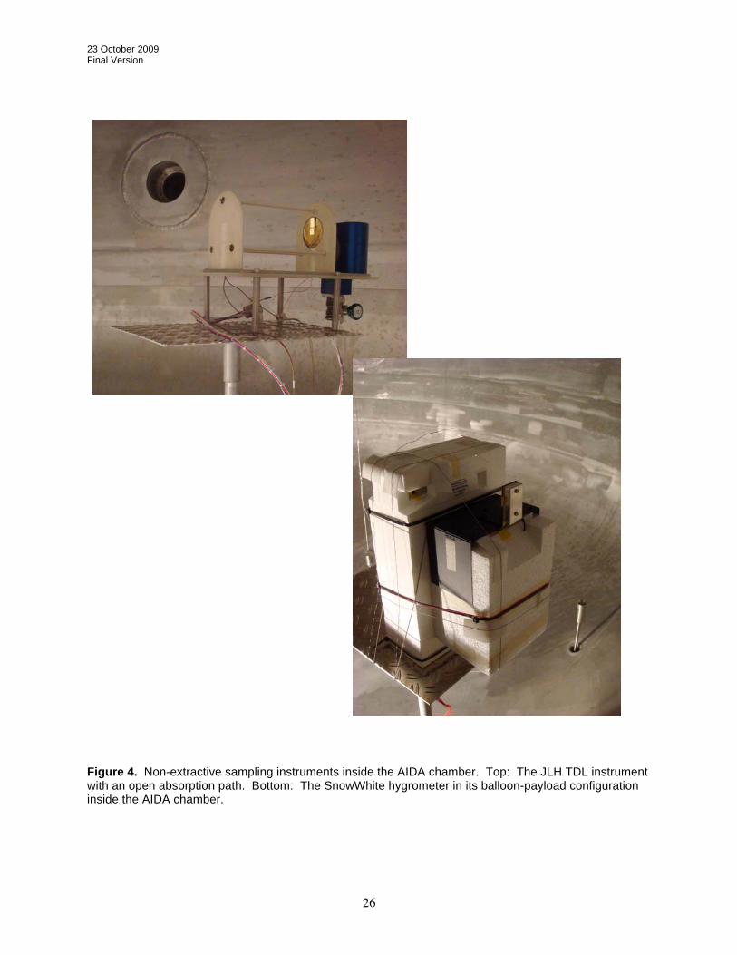
26
Figure 4. Non-extractive sampling instruments inside the AIDA chamber. Top: The JLH TDL instrument with an open absorption path. Bottom: The SnowWhite hygrometer in its balloon-payload configuration inside the AIDA chamber.

23 October 2009 Final Version
27
AIDA chamber conditions during AquaVIT
Figure 5. Conditions in the AIDA chamber during the static experiments. Top: Daily chamber temperature time series. Bottom: Daily chamber pressure time series.

23 October 2009 Final Version
28
AIDA chamber conditions during AquaVIT
Figure 6. Average AIDA chamber pressures and temperatures as a function of the water-vapor average reference value for the static experiment segments (see Table 4).
23 October 2009 Final Version
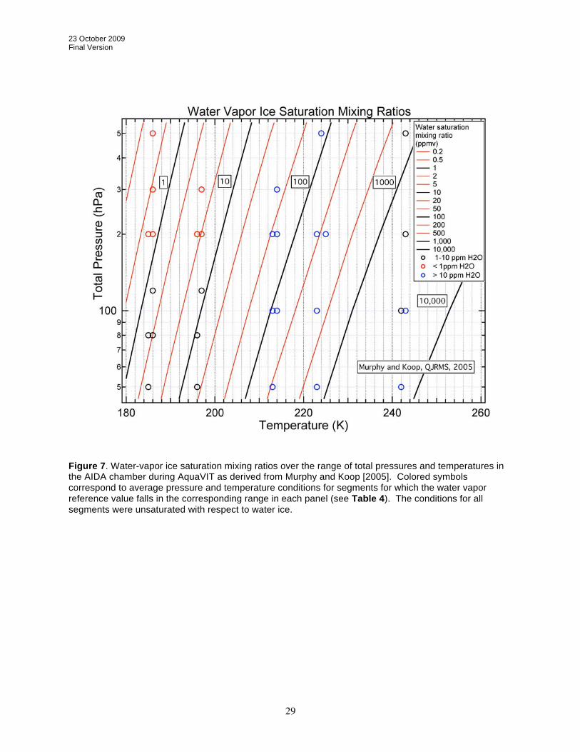
29
Figure 7. Water-vapor ice saturation mixing ratios over the range of total pressures and temperatures in the AIDA chamber during AquaVIT as derived from Murphy and Koop [2005]. Colored symbols correspond to average pressure and temperature conditions for segments for which the water vapor reference value falls in the corresponding range in each panel (see Table 4). The conditions for all segments were unsaturated with respect to water ice.

23 October 2009 Final Version
30
Figure 8. Time series of AIDA water vapor mixing ratios (1-s averages) as reported by many instruments during the static experiment on 15 October. The mixing ratios are shown with linear (top panel) and logarithmic (bottom panel) scales.

23 October 2009 Final Version
31
Figure 9A. Summary plot of the core instrument intercomparison results for the 5-day static experiment series. The instruments are identified on the left of each panel. Each panel is labeled by the range of reference water-vapor mixing ratios. The chamber pressure range is indicated by the symbol color. The symbols represent the average difference within a segment from the reference water vapor value for that segment. The segments varied from 900s to 3600s in length with most being 1800s (Table 4). The differences are plotted on separate log scales for values more than 1% above and below the reference value. Those differences equal to or less than 1% are plotted at a value of 1%. The average of all segments for an instrument is shown with the circle/plus symbol. Data are not available for all segments for each instrument. Instrument names in parentheses in a panel have no results in the associated mixing ratio range.

23 October 2009 Final Version
32
Figure 9B. Summary plot of static experiment results for core instruments shown as the % difference between values from the listed instruments and the corresponding reference values for three ranges of the reference values. A symbol represents the result for the segment number noted near the top axis. The use of a small symbol size for a segment indicates that the accuracy and precision cannot be defined based on the relationships in Table 3. Segment details are provided in Table 4. Colors represent the AIDA chamber average pressure during the segment. Differences less than or equal to 1% are plotted as a 1% value. Results for the non-core instruments are shown in Figure 10B with a different vertical axis range.

23 October 2009 Final Version
33
Figure 9C. Summary plot of static experiment results for the APicT instrument. The error bars represent the sum of accuracy and offsets as estimated for each segment from the values in Table 3. See caption of Figure 9B for further details.
Figure 9D. Summary plot of static experiment results for the CFH instrument. The error bars represent the sum of accuracy and offsets as estimated for each segment from the values in Table 3. See caption of Figure 9B for further details.

23 October 2009 Final Version
34
Figure 9E. Summary plot of static experiment results for the FISH-1 instrument. The error bars represent the sum of accuracy and offsets as estimated for each segment from the values in Table 3. See caption of Figure 9B for further details.
Figure 9F. Summary plot of static experiment results for the FISH-2 instrument. The error bars represent the sum of accuracy and offsets as estimated for each segment from the values in Table 3. See caption of Figure 9B for further details.

23 October 2009 Final Version
35
Figure 9G. Summary plot of static experiment results for the FLASH-B1 instrument. The error bars represent the sum of accuracy and offsets as estimated for each segment from the values in Table 4. See caption of Figure 9B for further details.
Figure 9H. Summary plot of static experiment results for the FLASH-B2 instrument. The error bars represent the sum of accuracy and offsets as estimated for each segment from the values in Table 3. See caption of Figure 9B for further details.

23 October 2009 Final Version
36
Figure 9I. Summary plot of static experiment results for the HWV instrument. The error bars represent the sum of accuracy and offsets as estimated for each segment from the values in Table 4. See caption of Figure 9B for further details.
Figure 9J. Summary plot of static experiment results for the JLH instrument. The error bars represent the sum of accuracy and offsets as estimated for each segment from the values in Table 3. See caption of Figure 9B for further details.

23 October 2009 Final Version
37
Figure 10A. Summary plot of static experiment results for the core and non-core instruments shown as the % differences between values from the listed instruments and the corresponding reference values for three ranges of the reference values. Each symbol represents a segment listed in Table 4. The circle/plus symbol denotes the instrument average for all segments. Colors represent the AIDA chamber average pressure during the segment. Differences less than or equal to 1% are plotted as a 1% value. The results for the core instruments are also shown in Figure 9A. Instrument names in parentheses indicated that no data or insufficient data were available for statistical analyses in the indicated mixing ratio range. In addition, no CLH data are available for the upper two panels.
23 October 2009 Final Version
38
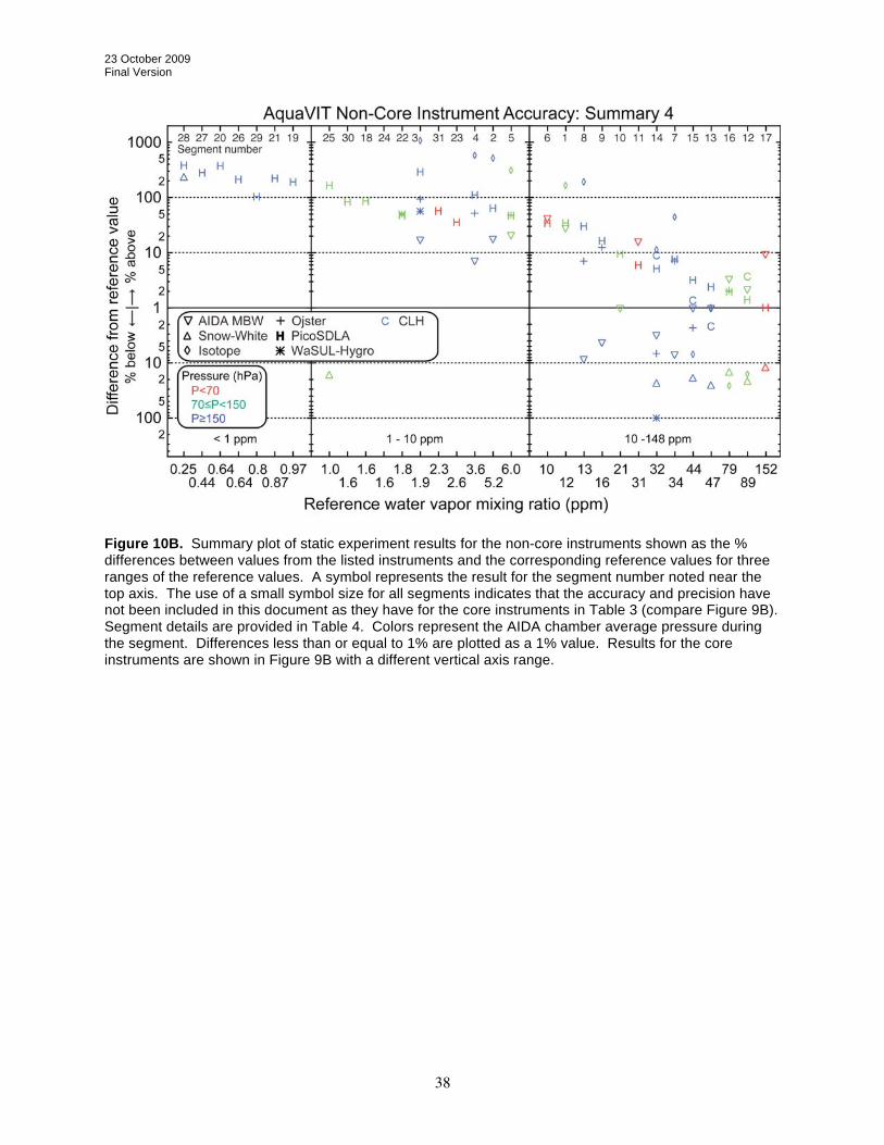
Figure 10B. Summary plot of static experiment results for the non-core instruments shown as the % differences between values from the listed instruments and the corresponding reference values for three ranges of the reference values. A symbol represents the result for the segment number noted near the top axis. The use of a small symbol size for all segments indicates that the accuracy and precision have not been included in this document as they have for the core instruments in Table 3 (compare Figure 9B). Segment details are provided in Table 4. Colors represent the AIDA chamber average pressure during the segment. Differences less than or equal to 1% are plotted as a 1% value. Results for the core instruments are shown in Figure 9B with a different vertical axis range.

23 October 2009 Final Version
39
Figure 10C. Summary plot of static experiment results for the MBW-373LX instrument. No error bars are shown because the accuracy and offsets estimates are not available for each segment. See caption of Figure 10B for further details.
Figure 10D. Summary plot of static experiment results for the SnowWhite instrument. No error bars are shown because the accuracy and offsets estimates are not available for each segment. See caption of Figure 10B for further details.

23 October 2009 Final Version
40
Figure 10E. Summary plot of static experiment results for the ISOWAT instrument. No error bars are shown because the accuracy and offsets estimates are not available for each segment. See caption of Figure 10B for further details.
Figure 10F. Summary plot of static experiment results for the OJSTER instrument. No error bars are shown because the accuracy and offsets estimates are not available for each segment. See caption of Figure 10B for further details.

23 October 2009 Final Version
41
Figure 10G. Summary plot of static experiment results for the PicoSDLA instrument. No error bars are shown because the accuracy and offsets estimates are not available for each segment. See caption of Figure 10B for further details.
Figure 10H. Summary plot of static experiment results for the WaSul-Hygro2 instrument. No error bars are shown because the accuracy and offsets estimates are not available for each segment. See caption of Figure 10B for further details.

23 October 2009 Final Version
42
Figure 10G. Summary plot of static experiment results for the CLH instrument. No error bars are shown because the accuracy and offsets estimates are not available for each segment. See caption of Figure 10B for further details

23 October 2009 Final Version
43
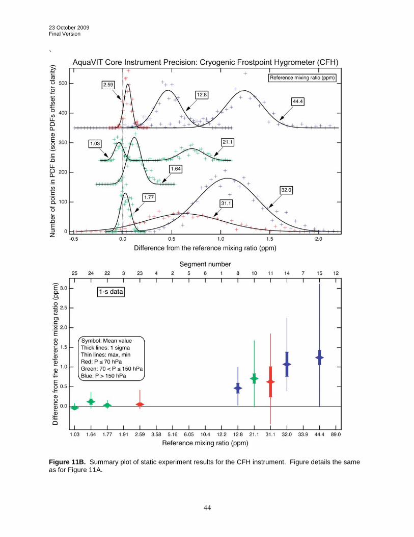
Figure 11A. Summary plot of static experiment results for the APicT instrument. Top: Gaussian fits to the probability distribution functions (pdfs) of differences from the reference value function derived for each segment from the core instruments. The pdfs are derived from 1-s time series data. Legend boxes indicate the reference water vapor value for each segment (see Table 4). PDFs and fits are offset in the vertical for clarity. Bottom: Plot of mean (symbols) and max and min (thin lines) differences from the reference values and 1- precision (thick line) as defined in Table 5 footnote. Color indicates pressure range in both top and bottom panels.
23 October 2009 Final Version
44
`
Figure 11B. Summary plot of static experiment results for the CFH instrument. Figure details the same as for Figure 11A.

23 October 2009 Final Version
45
Figure 11C. Summary plot of static experiment results for the FISH-1 instrument. Figure details the same as for Figure 11A.

23 October 2009 Final Version
46
Figure 11D. Summary plot of static experiment results for the FISH-2 instrument. Figure details the same as for Figure 11A.

23 October 2009 Final Version
47
Figure 11E. Summary plot of static experiment results for the FLASH-B1 instrument. Figure details the same as for Figure 11A.
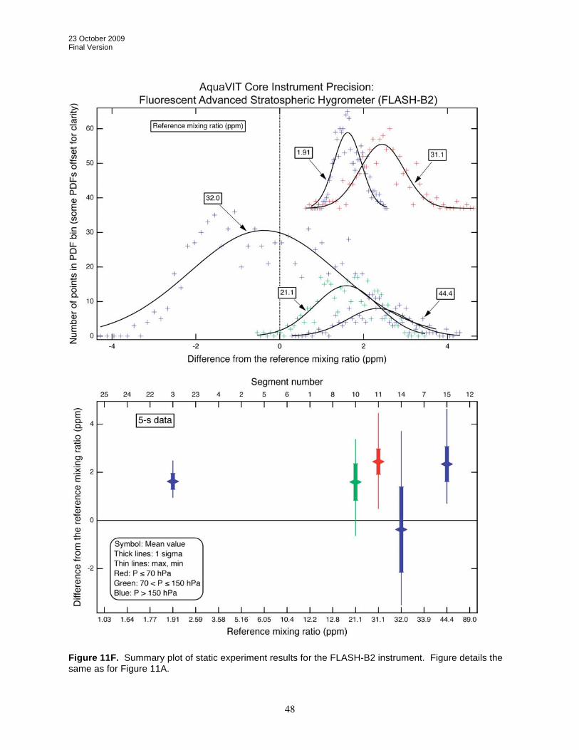
23 October 2009 Final Version
48
Figure 11F. Summary plot of static experiment results for the FLASH-B2 instrument. Figure details the same as for Figure 11A.

23 October 2009 Final Version
49
Figure 11G. Summary plot of static experiment results for the HWV instrument. Figure details the same as for Figure 11A.

23 October 2009 Final Version
50
Figure 11H. Summary plot of static experiment results for the JLH instrument. Figure details the same as for Figure 11A.

23 October 2009 Final Version
51
Figure 12A. Summary plot of static experiment results for the APicT instrument. Top: Precision results using the 1-s time series data as shown in Figure 11. Bottom: Precision results using the 5-s time series data. Other figure details the same as for Figure 11A.

23 October 2009 Final Version
52
Figure 12B. Summary plot of static experiment results for the CFH instrument. Top: Precision results using the 1-s time series data as shown in Figure 11. Bottom: Precision results using the 5-s time series data. Other figure details the same as for Figure 11A.

23 October 2009 Final Version
53
Figure 12C. Summary plot of static experiment results for the FISH-1 instrument. Top: Precision results using the 1-s time series data as shown in Figure 11. Bottom: Precision results using the 5-s time series data. Other figure details the same as for Figure 11A.

23 October 2009 Final Version
54
Figure 12D. Summary plot of static experiment results for the FISH-2 instrument. Top: Precision results using the 1-s time series data as shown in Figure 11. Bottom: Precision results using the 5-s time series data. Other figure details the same as for Figure 11A.

23 October 2009 Final Version
55
Figure 12E. Summary plot of static experiment results for the HWV instrument. Top: Precision results using the 1-s time series data as shown in Figure 11. Bottom: Precision results using the 5-s time series data. Other figure details the same as for Figure 11A.

23 October 2009 Final Version
56
Figure 12F. Summary plot of static experiment results for the JLH instrument. Top: Precision results using the 1-s time series data as shown in Figure 11. Bottom: Precision results using the 5-s time series data. Other figure details the same as for Figure 11A.

23 October 2009 Final Version
57
Correlation Plot of AquaVIT Core Instruments
Figure 13A. Summary plot of the correlations of the core instruments with the water vapor reference values in the range 0.9 – 10 ppm H2O. Data from the FLASH-B1/B2 instruments are not available for this mixing ratio range.

23 October 2009 Final Version
58
Figure 13B. Correlation plot of CFH and APicT data from all segments. Data points are derived from filtering the full instrument time-series data with a 50-s median filter.
Figure 13C. Correlation plot of FISH-1 and APicT data from all segments. See Figure 13B for further details.
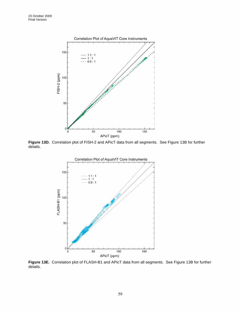
23 October 2009 Final Version
59
Figure 13D. Correlation plot of FISH-2 and APicT data from all segments. See Figure 13B for further details.
Figure 13E. Correlation plot of FLASH-B1 and APicT data from all segments. See Figure 13B for further details.
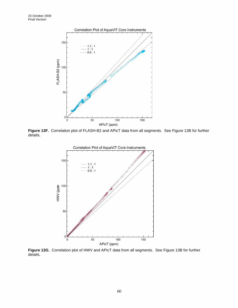
23 October 2009 Final Version
60
Figure 13F. Correlation plot of FLASH-B2 and APicT data from all segments. See Figure 13B for further details.
Figure 13G. Correlation plot of HWV and APicT data from all segments. See Figure 13B for further details.

23 October 2009 Final Version
61
Figure 13H. Correlation plot of JLH and APicT data from all segments. See Figure 13B for further details.

23 October 2009 Final Version
62
Appendix A. Core instrument descriptions A1. APicT (TDL) Volker Ebert*, Christian Lauer, Stefan Hunsmann, Harald Saathoff, Steve Wagner, University of Heidelberg and Forschungszentrum Karlsruhe, Germany. *Now at Physikalisch-Technische Bundesanstalt (PTB), National Metrology Institute of Germany, Germany. The AIDA-PCI-in-cloud-TDL (APicT) spectrometer is a fiber-coupled, diode laser based, high spectral resolution absorption spectrometer to selectively detect interstitial water vapor inside clouds and to continuously determine absolute water vapor volume fraction inside the AIDA main chamber. It is designed to investigate cloud formation within AIDA and thus can be used in particle-free conditions and especially when clouds are formed within the APicT absorption path. Main goal of the instrument design was – aside of high chemical selectivity and sensitivity, sufficient temporal resolution – to achieve a highly accurate, absolute, water vapor measurement by complete avoidance of gas sampling, gas treatment and particularly without a calibration of the instrument response, i.e. by using water vapor generators. The APicT instrument (developed in 2002 [1]) combines PCI’s experience in very robust, laser-based, open-path species diagnostics in large-scale combustion processes [2] and a previously developed stratospheric, balloon-borne, open-multi-path instrument (CHILD) for simultaneous H2O/CH4 detection [3] with knowledge on highly stable open White-type [4] white multi-path cells developed by FZ Karlsruhe [5]. Since 2003 APicT has been used in more and more cloud formation studies at AIDA in order to determine absolute water vapor and super saturation values dynamics during cloud formation [5-9]. ApicT uses direct absorption spectroscopy [2,10] (instead of the more common 2f wavelength modulation technique [11]) to avoid calibration, while simultaneously permitting an efficient correction for the spectrally broad band optical losses caused by the cloud particles; This technique has been perfected for measurements in severely dust laden combustion chambers [2,12]. The H2O vapor molecules are detected via the (110 -211) line (7299 cm-1) in the n1+n3 combination band (or for higher H2O concentrations via the (211 322) line in the 2n1-overtone-band) both around at 1.37 m [1,13]. APicT consist of three basic parts [1,13]: A: The outer part, placed within the user accessible space outside the AIDA insulation chamber, contains a fiber-coupled temperature-stabilized distributed feedback (DFB) diode laser module in a N2-purged container and all electronics (Laser/Peltier driver, signal generator, detector preamplifiers, data acquisition, and computer); B: The middle part, a cryogenic transfer optic (including two detectors for I and I0), is directly attached to the outside wall of the AIDA inner chamber. Using the fiber from the laser module and a lens collimator a free space laser beam is formed, which is then focused through wedged CaF2 windows into the absorption cell in the inner chamber. Through a second identical window the laser light behind the measurement zone is collected and directed onto an uncooled InGaAs detector (1mm diam.) using a 1” spherical mirror. In the middle section, which is at atmospheric pressure but at AIDA chamber temperatures, the total path length of the free space beam from the fiber to the detector is 36 cm. Part C is the cryogenic, open, White-type multi-path absorption cell with heated mirrors. The cell is permanently mounted onto the walls (3.74m mirror separation) inside the AIDA chamber and enables path lengths of up to 250 m (82m mostly used during Aquavit). For the measurements the laser is scanned across the target line with a repetition frequency of 139 Hz. The resulting absorption profiles are coadded up to 100 times (i.e. 1-2 s time resolution). The averaged in situ signal is corrected for optical losses, electrical offsets, converted from time to frequency space (using the laser tuning characterization) and evaluated using the ideal gas law and an extended Lambert-Beer law [1,2,10,12,13], a Voigt line shape model and a non-linear Levenberg-Marquardt fitting algorithm, taking into account measured pressure, temperature and absorption path length inside AIDA, a highly precise characterization of the dynamic laser tuning (using a 10 cm air-spaced precision etalon), as well as our measured [14] air broadening coefficient (gair=0,0981 ± 0,0002 cm-1/atm at 296K) and temperature coefficient (n=0,74 ± 0.01) and the tabulated H2O line strength from HITRAN2004, which we verified during AIDA measurements within a ±3% uncertainty [14]. For very low H2O concentrations we also

23 October 2009 Final Version
63
correct for parasitic absorption effects in the middle section of the spectrometer by using either a secondary detector channel on the cryo transfer optics board, or the known ratio between the parasitic and the inner absorption path (0,36m/82m). No calibration or scaling parameters are used. With that procedure/instrument we can cover concentrations from 10,000 to 1 ppm at pressure/temperature ranges from 1000/1 mbar 300/180K and achieve precisions (1s) in the 20 ppb range [13]. The absolute accuracy we estimate from an error budget to be below 5% and dominated by the line strength uncertainty. Optical losses by cloud particles of 99% have been handled without additional systematic errors (even higher losses of 99,99% have been compensated for in combustion applications using dedicated DSP based electronics [15]). The instrument and parts thereof have been extensively validated for absolute accuracy: Tuning accuracy has been checked via Doppler line shapes ( 0.15% deviation). The software and evaluation procedure of an identical open path laser spectrometer for CH4 was validated by comparing measured atmospheric levels of background CH4 with a NOAA calibrated, extractive gas chromatograph ( <1% average deviation over 36 hours) [16]; H2O vapor values were compared at AIDA with Frostpoint (MBW) and Lyman alpha instruments (FISH) during particle free conditions ( typically < 3% deviation) [14]. The performance during the static experiments (first week) of the Aquavit campaign was hampered due to a software problem which caused a sensitivity loss of nearly a factor of 10. This had to be compensated by reducing the instruments temporal response adequately. During the dynamic experiments (second week) this error had been removed. A1.1 APict ice-saturation experiments During the AquaVIT dynamic experiments, dense ice clouds were present in the AIDA chamber during 10 time segments (600 s to 2400 s duration) with almost constant pressure and temperature. During these time periods, the average relative humidity inside the chamber was maintained at ice-saturated conditions at the respective gas temperature. At constant pressure and temperature conditions, the variability of the gas temperatures measured throughout the chamber volume is typically less than ±0.2 °C, which means that the variability of the water saturation pressure above the ice-crystal phase is less than about ±3%. The average values of water vapor and temperature in the ice-saturated segments were in the range 0.01-40 Pa and 185-243K, respectively. Figure A1.1 (top) shows the percentage differences between the APicT water vapor partial pressures and ice-saturation values derived from measured temperatures for segments in the dynamic experiments (Table 1). Figure A1.1 (bottom) shows the water vapor partial pressures from APicT measurements and ice-saturation calculations (Ice sat), and the chamber water vapor mixing ratio for each segment. During the segments, the water-vapor partial pressure measured in situ with the APicT instrument deviated by less than ±3% from the ice-saturation pressures calculated from laboratory vapor pressure relations reported by Murphy and Koop (2005) (Figure A1.1). The laboratory relations have an estimated uncertainty of ±1%. APicT water retrievals are insensitive to the presence of ice clouds under the experiment conditions. The error bars in the figure are derived from the widths of the Gaussian fits to the probability distribution functions of 1-s APicT and ice saturation water vapor partial pressure data in each segment (see AquaVIT dynamic experiments summary (in preparation)). Within its estimated uncertainty limits of about 5%, APicT correctly measured the expected ice saturation conditions, with a slight tendency of a low bias at the higher water concentrations and temperatures (i.e., low segment numbers), and a high bias at the lower water concentrations and low temperatures (i.e., at high segment numbers). A1.2 References [1] Dissertation Carsten Giesemann, „Entwicklung und Einsatz eines Diodenlaserspektrometers zum
quantitativen In-situ-Nachweis von Methan und Wasser in der Stratosphäre“, FAKULTÄT FÜR CHEMIE
UND GEOWISSENSCHAFTEN, UNIVERSITÄT HEIDELBERG (2003). [2] C. Schulz, A. Dreizler, V. Ebert, J. Wolfrum , "Combustion Diagnostics" in Springer Handbook of
Experimental Fluid Dynamics, Editors C. Tropea, J. Foss, A. Yarin, 1241-1316 (2007). [3] W. Gurlit, J. P. Burrows, R. Zimmermann, U. Platt, C. Giesemann, J. Wolfrum, V. Ebert, “Light-
Weight Diode Laser Spectrometer for Balloon-Borne Measurements of Water Vapor and Methane”, Applied Optics 44, 91-102, 1 January 2005.
[4] J.U. White, “Long optical path of large aperture” J Opt Soc Am, 32, 285-288 (1942).

23 October 2009 Final Version
64
[5] R. Wagner, S. Benz, H. Bunz, O. Möhler, H. Saathoff, M. Schnaiter, T. Leisner, V. Ebert, “Infrared optical constants of highly diluted sulfuric acid solution droplets at cirrus temperatures”, J Phys Chem A , 112, 11661 (2008).
[6] O Möhler, S Benz, H Saathoff, M Schnaiter, R Wagner, J Schneider, S Walter, V Ebert and S
Wagner, The effect of organic coating on the heterogeneous ice nucleation efficiency of mineral dust aerosol, Environment Research Letters, 3 (2008) 025007 (8pp).
[7] O. Möhler, D. G. Georgakopoulos, C. E. Morris, S. Benz, V. Ebert, H. Saathoff, M. Schnaiter, and R. Wagner , Heterogeneous ice nucleation activity of bacteria: New laboratory experiments at simulated cloud conditions , Biogeosciences, 5, 1425–1435, 2008.
[8] O. Möhler, S. Büttner, C. Linke, M. Schnaiter, H. Saathoff, O. Stetzer, R. Wagner, M. Krämer, A. Mangold, V. Ebert, and U. Schurath, ” Effect of sulfuric acid coating on heterogeneous ice nucleation
Figure A1.1. (Top) Differences between APicT water vapor partial pressures and those calculated from ice-saturation at measured temperatures (top axis) for AquaVIT dynamic experiment segments. (Bottom) Water vapor partial pressures vs. dynamic segment number as calculated (ice sat) and as measured by APicT. Also shown are water vapor mixing ratios in the chamber (right hand axis).

23 October 2009 Final Version
65
by soot aerosol particles ”, Journal of Geophysical Research, 110, D11210, doi:10.1029/2004JD005169. (2005).
[9] A. Mangold, R. Wagner, H. Saathoff, U. Schurath, C. Giesemann, V. Ebert, M. Krämer, O. Möhler, Experimental investigation of ice nucleation by different types of aerosols in the aerosol chamber AIDA: implications to microphysics of cirrus clouds, Meteorologische Zeitschrift, Volume 14, Number 4, August 2005, pp. 485-497(13).
[10] V. Ebert, J. Wolfrum “Absorption spectroscopy“ in Optical Measurements- Techniques and Applications, 2nd corr. edition, F. Mayinger, O. Feldmann (Eds.), (Heat and Mass Transfer), Springer Verlag, Heidelberg, München, 227- 265 (2001).
[11] T. Fernholz, H. Teichert, V. Ebert, “Digital, Phase-Sensitive Detection for In Situ Diode Laser Spectroscopy under Rapidly Changing Transmission Conditions”, Appl. Phys B 75 2-3, 229-236 (2002).
[12] H. Teichert, T. Fernholz, V. Ebert, “In situ Measurement of CO, H2O and Gas Temperature in a Lignite-Fired Power-Plant“, Applied Optics 42, 2043-2051 (2003).
[13] V. Ebert, H. Teichert, C. Giesemann, H. Saathoff, U. Schurath, ”Fiber-coupled In situ-Laser Absorption Spectrometer for the selective Detection of Water Vapor Traces down to the ppb-Level ”, Technisches Messen 72, 1, 23-30 (2005).
[14] S. Hunsmann, S. Wagner, H. Saathoff, O. Möhler, U. Schurath, V. Ebert, “Measurement of the temperature dependence of line strength and pressure broadening coefficients of water absorption lines in the 1.4 m-Band”, VDI Berichte 1959 VDI Verl. - Düsseldorf, 149-164, 2006.
[15] A. R. Awtry, B. T Fisher, R. A. Moffatt, V. Ebert and J. W. Fleming, Simultaneous Diode Laser Based In Situ Quantification of Oxygen, Carbon Monoxide, Water Vapor, and Liquid Water in a Dense Water Mist Environment, Proc. Comb. Inst. 31, (2006), 799-806.
[16] C. Lauer, D. Weber, S. Wagner, V. Ebert, Calibration Free Measurement of Atmospheric Methane Background via Tunable Diode Laser Absorption Spectroscopy at 1.6 m, Laser Applications to Chemical, Security and Environmental Analysis (LACSEA), St. Petersburg, Florida, USA, March 17-20, 2008 Paper no. LMA2 -- or -- Dresdner Beiträge zur Sensorik, Hrsg. G. Gerlach, P, Hauptmann, Band 29, ISBN 978-3-940046-45-1, S. 7-10 (2007).

23 October 2009 Final Version
66
A2. Cryogenic Frostpoint Hygrometer (CFH)
Holger Vömel, Meteorologisches Observatorium Lindenberg, German Weather Service, Lindenberg, Germany A2.1 Balloon Instrument A2.1.1 Instrument description The Cryogenic Frostpoint Hygrometer (CFH) is a small balloon borne instrument that measures water vapor continuously between the surface and the middle stratosphere (Vömel et al., 2007) (See Figure A2.1). It is based on the chilled mirror principle and measures the temperature of a mirror carrying a thin dew or frost layer that is maintained in equilibrium with the ambient water vapor. The optical phase-sensitive detector measures the bulk reflectivity of the mirror, while the microprocessor feedback controller regulates the mirror temperature such that the bulk reflectivity and hence the condensate layer remain constant. Under this condition the condensate layer on the mirror is in thermal equilibrium with the vapor phase of the air passing over the mirror. The mirror temperature is then equal to the ambient dew point or frost point temperature and the water vapor mixing ratio and relative humidity can be calcu-lated from this measurement using a variation of the Clausius-Clapeyron equation. The CFH is currently flown with an ECC ozone sonde, GPS, and a Vaisala RS80 radiosonde, which is used as data transmitter. Therefore, in addition to water vapor mixing ratio, every CFH payload provides ozone mixing ratio and RS80 pressure, temperature and humidity data, which are used to determine altitude, potential temperature and mixing ratio.
A2.1.2. Instrument characteristics Vertical measurement range: 0 km to ~28 km Dew point or frost point detection range: >+25°C to <-95°C Mixing ratio detection range: >25000 ppmv to <0.8 ppmv Dew point or frost point uncertainty: 0.5°C Mixing ratio uncertainty: ~ 3.5 % (surface), ~9% (tropopause), ~11% (28 km) Vertical resolution: <~ 10 m (troposphere) to < ~ 100 m (stratosphere) CFH instrument weight: 400 g CFH + ECC + RS80 payload launch weight: 1500 g A2.2 CFH configuration during AquaVIT A2.2.1 Laboratory instrument configuration During AquaVIT a laboratory version of the balloon instrument was used. This version was required because
Figure A2.1. Schematic of the Cryogenic Frostpoint Hygrometer (CFH).

23 October 2009 Final Version
67
of the need to connect the CFH to a vacuum system, as well as the need to measure pressure and frostpoint temperature separately. For the laboratory instrument, a stainless steel sensor housing was built, which has largely the same geometry as the balloon borne instrument, but allows the connection to a vacuum system and a separate pressure measurement near the sampling volume. The optical path of the lab instrument was nearly identical to the balloon instrument, with the only difference being that the detector lens was slightly recessed to allow the addition of a sapphire window, which acted as vacuum seal. The detector and electronics was taken from a balloon instrument and was therefore identical to the balloon version. The mirror holder was made of a thin walled stainless steel tube, which was glued to the mirror disk and acted both as vacuum seal and thermal insulator to the sensor housing. The dimensions of the mirror, mirror stem and heater coil are identical to the balloon instrument as are the location of the thermistors. This assures that the thermal properties of the assembly are the same as those of the balloon instrument. The cold finger, which is the part of the mirror assembly that is immersed in the cryogen, was longer than that of the balloon instrument, since accessibility to the sensor housing required a larger separation of the cryogen container from the sensor housing. The cooling rate of the instrument, however, is determined by the dimensions of the thin mirror stem, which remained unchanged. Thus the laboratory instrument differs from the balloon instrument largely in the use of different materials, which allowed the connection to a vacuum system. All key parameters of the laboratory version are identical to those in the balloon instrument The pressure was measured using a Baratron pressure sensor, which was attached to a separate fitting about 20 cm downstream of the mirror. The flow tube maintained the 1” diameter through the frostpoint hygrometer and the pressure sensor section and no pressure gradient is expected under this configuration. A2.2.2 Laboratory instrument additions The new laboratory instrument allowed several additions, which are not implemented in the balloon instrument. The most important optional addition is that the detector LED and detector photodiode could be moved from the specular position (about 85º incidence angle) to a position with about 45º incidence angle. For this purpose additional access holes where installed, which were vacuum sealed using small sapphire windows. Rotationally offset by 90º from this detection axis two white LED were placed to illuminate the mirror and frost layer. This allowed a visual observation of the mirror and frost coverage through the main sapphire window. Since the CFH is insensitive to ambient light the addition of the white light LEDs did not impact the detector operation. The relocation of the detector LED and photodiode from the specular axis resulted in some loss of signal. This reduced signal loss is compensated for by referencing the frost coverage to the clear mirror signal. It did not impact the operation of the CFH or lead to a change in PID (Proportional, Integrating, Differentiating) controller settings. To verify the mirror temperature measurement a second thermistor was installed in the mirror. The radial distance of the second thermistor is similar to that of the main mirror thermistor. This thermistor was measured independently with a second CFH board, which was not involved in the normal feedback loop. A2.3 CFH Operation during AquaVIT A2.3.1 Cryogen The CFH during AquaVIT was operated using liquid nitrogen. Since it is significantly colder than trifluoromethane, which is used in a balloon sounding, a Teflon sleeve was placed over the cold finger to reduce the heat transfer into the cryogen. The Teflon sleeve nearly compensated the colder temperature and liquid nitrogen and these two changes led to heater currents, which were comparable to those observed in flight. The cryogen container capacity was about twice that of the balloon instrument, however, the heat capacity of liquid nitrogen is less than that of trifluoromethane. Thus liquid nitrogen had to be added about every 2.5 hours. A2.3.2 Data acquisition Data acquisition was done using a Labview program, which recorded the 7 Hz output of the CFH. In addition to the mirror temperature, this program recorded optics voltage, detector temperature, heater output and pressure. Due to a software bug, which was solved only after the completion of AquaVIT, a buffer overflowed about every two hours and data acquisition had to be restarted. During the time of the

23 October 2009 Final Version
68
buffer overflow, data acquisition was increasingly delayed, in some case up to 30 seconds before restart. This delay did not impact any of the static experiments, but it did impact some of the dynamic experiments during the second week, where delays were observed during some cloud experiments. These delays resulted in a belated recording of the instrument response, not in a smoothing of the instrument response. The restart of the data acquisition also caused a reset of the CFH, which led to a clearing pulse associated with some short loss of measurements. A2.3.3 Mirror cleaning During the first week of operation the CFH remained connected to the AIDA chamber, was not opened, and the mirror was not cleaned during this set of experiments. A slight film deposit was observed on the fifth day of the first week, which prompted a mirror cleaning after the morning experiments. This initial cleaning led to a very serious instrument issue, which was resolved only with the completion of this experiment day. No measurements exist on the afternoon of the fifth and last day of static experiments. During the dynamic experiments of the second week the mirror was cleaned at least after the completion of every experiment day. Cleaning was done using cotton swabs and methanol, while monitoring the optics signal. This procedure is identical to the pre-launch instrument preparation for a balloon sounding. Cleaning was completed when the reflectivity signal was maximized. A2.3.4 Mirror clearing The frost layer was frequently cleared by heating the mirror to about 20ºC and letting the condensate layer evaporate completely. This happened typically within a second. After mirror clearing the instrument resumed normal operation with a newly formed frost layer. During days two and three of the first week and during days one through three of the second week the frost layer could be condensed with the water vapor available from the AIDA chamber. During the experiments with the lowest frostpoint temperatures (days four and five of both weeks), the frost layer could not be condensed with the water vapor coming from the AIDA chamber. On day four of the static experiments this was unsuccessfully attempted. Frost formation took over 30 minutes and the inappropriate controller settings immediately removed this frost layer once it was detected. This was attempted twice and then aborted. For these days, water vapor was added to the system through a leak valve, which allowed the CFH to create a frost layer at a higher water vapor concentration than was available from the AIDA chamber. Establishing control at the higher water vapor concentrations using the leak valve took about one second. Closing the leak valve with continuous control took about one minute. Thus it took about two to three minutes to clear the mirror to re-condense the frost layer and to bring the CFH into stable control at the water vapor concentration during the days of the lowest frostpoint temperatures. The times between mirror clears varied between several minutes to about two hours. The upper limit was set by the buffer overflow problem of the acquisition software. During a balloon sounding, which typically takes 90 minutes on ascent and 30 to 45 minutes on descent two mirror clears happen. Thus the time between mirror clears during AquaVIT is comparable to that of a balloon sounding. A2.4. CFH Experiments in addition to the AquaVIT program A2.4.1 Detector location and microscope observations During the second and third day of AquaVIT both detection axes were used to study if the reduced signal in the off-specular detector configuration caused any negative impacts. No difference between these two configurations was observed. Starting on day four of AquaVIT all experiments were run using the off-specular detector configuration. For nearly all measurements visual images of the frost layer exist. These visual images can be used as an independent quantification of a stable frost layer. A2.4.2 Controller settings During the first week of operation the PID parameters used to run the CFH were those used by the balloon instrument, which depend only on frostpoint temperature. During the second week a number of experiments were performed with changed parameters to study whether the PID parameters could be optimized. All of these experiments remained inconclusive and aside from occasional controller
23 October 2009 Final Version
69
instability, no changes in instrument performance were observed. A2.4.3 Frost layer morphology The mirror clear capability was used to study the influence of different frost layer morphologies. These experiments showed that the frost layer morphology can have a significant influence on the performance of a frostpoint hygrometer. However, all data submitted to the AquaVIT archive used a frostlayer consistent with one that would have formed during a routine CFH sounding. A2.4.4 Liquid – ice transition The AquaVIT experiment focused on low water vapor concentrations, which translated to low frostpoint temperatures. However, in the atmosphere there exists a frostpoint temperature range in which the phase of the mirror condensate is not uniquely defined and in which the measurement of reflectivity does not provide sufficient data to distinguish the condensate phase. The transition between liquid phase and solid phase of the condensate on the mirror was studied after the completion of one AquaVIT experiment day. These experiments clearly show that the liquid to ice transition for the mirror condensate has to be carefully considered in any frostpoint hygrometer measurement and that it impacts a sounding beyond the region of ambiguity. A2.4.5 Flow rate dependency The exhaust line of the lab CFH was connected to the vacuum system using a needle valve. Using this valve the flow through the instrument could be varied to study any possible flow rate dependency of the measurement. No such dependency could be found. In fact, flow rate variations led to strong pressure variations in the instrument as well as to strong frostpoint temperature variations. Measured frostpoint changes were as fast as pressure changes while the needle valve was either opened or closed. However, the changes in frostpoint perfectly canceled changes in pressure leading to constant mixing ratios throughout these experiments. This was taken as confirmation that the instrument responds as it should to changes in partial pressure, while maintaining a constant mixing ratio. A2.4.6 PTB permeation source The Physikalisch Technische Bundesanstalt (PTB) provided a water vapor permeation source, which was used as independent reference on day four of the second week of experiments. Strong outgassing was observed after initial setup, however, after several hours of measurement a good agreement between the permeation source and the CFH measurement was achieved. A2.5 References Vömel, H., D. E. David, and K. Smith, Accuracy of tropospheric and stratospheric water vapor measurements by the cryogenic frost point hygrometer: Instrumental details and observations, J. Geophys. Res., 112, D08305, doi:10.1029/2006JD007224 (2007).

23 October 2009 Final Version
70
A3. Fast In situ Stratospheric Hygrometer (FISH-1 & FISH-2) Cornelius Schiller, Martina Krämer, Armin Afchine, Reimar Bauer, Jessica Meyer, Nicole Spelten, Andres Thiel, Miriam Kübbeler, Forschungszentrum Jülich, Jülich, Germany. A3.1 Instrument description The Fast In situ Stratospheric Hygrometer (FISH), developed at the Forschungszentrum Jülich (Germany), is based on the Lyman- photofragment fluorescence technique. FISH has been used in several balloon- and aircraft campaigns and compared to many other hygrometers during atmospheric measurements. The instrument is described in detail by Zöger et al. [1999]. FISH consists of a closed, vacuum-tight fluorescence cell, a Lyman- radiation source, a PMT in photon-counting mode, detectors to monitor the VUV radiation output of the Lyman- lamp, and a mirror drive that controls the measuring cycle: the determination of the fluorescence Ng and background count rate Nu and of the lamp intensity I0. The water vapour mixing ratio is determined via [H2O] = ck·(Ng-fu·Nu)/I0. The coefficients ck and fu are determined in the calibration procedure. The calibration of FISH is done in regular intervals between the measurement deployments using a calibration bench, consisting of a humidity mixing system and a frost point hygrometer (MBW DP30) as a reference instrument [Zöger et al., 1999; Meyer et al., 2009]. A calibration is done by varying the pressure (typically 80 – 500 hPa) and mixing ratio (1 – 500 ppmv) to cover the relevant range of the atmospheric measurements. A3.2 Performance during AquaVIT During AquaVIT, two instruments were operated, i.e. FISH-1 (designed for and used on Lear Jet missions; here operated from the upper AIDA platform) and FISH-2 (designed for and used on Geophysica and Falcon missions; here operated from the lower AIDA platform). Both instruments are almost identical concerning the core components; however the lamp of FISH-1 couldn’t be tuned in its optimum mode resulting in a lower signal-to-noise ratio compared to FISH-2. Both hygrometers worked nominally during all AquaVIT experiments except for October 22, as the high H2O concentrations during that particular dynamic instruments caused optically thick conditions for FISH. Flow rates on the order of 10 SLM could be achieved and are comparable to those during aircraft operations; only a few periods with flow rates below 5 SLM had to be removed for FISH-2 when contamination could not be excluded. Calibrations were carried out on October 10, 15, 20, 21, 24 and 30. No significant drift of the calibration factors ck and fu could be detected over the AquaVIT period, the reproducibility of ck was better than 3% (FISH-2) and 4% (FISH-2) for individual calibrations [Meyer, 2008]. The used MBW DP30 reference hygrometer has been calibrated by the manufacturer traceable to NPL standards a few months before AquaVIT. During AquaVIT, this DP30 was also compared to the secondary PTB standard (Appendix C). From this comparison, the DP30 accuracy was determined to be 2% in VMR [Meyer, 2008; Meyer et al., 2009]. A3.3 Lessons learned during AquaVIT Analysing the unexpected low bias of FISH data compared to the other AquaVIT core instruments at high mixing ratios and low pressure, additional laboratory calibrations have been carried out over an extended pressure range in the home laboratory. Here, a pressure dependence became apparent which is likely caused by absorption of the tails of the Lyman- line by O2 [Meyer et al., 2009]. This pressure dependence can be corrected introducing a pressure dependence of ck (not done for the data shown in this paper). The airborne data of FISH however, are not impacted by this effect as such conditions, i.e. mixing ratios of several ten to hundreds ppmv at pressure below 100 hPa, do not occur in the atmosphere. A3.4 References Meyer, J., Vergleich und Charakterisierung stratosphärisch messender in-situ Hygrometer (in German),
Diploma Thesis University Aachen, 2008.

23 October 2009 Final Version
71
Meyer, J., et al., Calibration of a flurorescence hygrometer at low water mixing ratios, in preparation, Atmos. Meas. Tech. (2009).
Zöger, M., et al., Fast in situ stratospheric hygrometers: A new family of balloonborne and airborne Lyman- photofragment fluorescence hygrometers, J. Geophys. Res., 104, 1807-1816 (1999).

23 October 2009 Final Version
72
A4. FLuorescent Advanced Stratospheric Hygrometer for Balloon (FLASH-B1 & FLASH-B2) Sergey Khaykin, Leonid Korshunov, Central Aerological Observatory, Moscow, Russia. A4.1 Instrument description The FLuorescent Advanced Stratospheric Hygrometer for Balloon (FLASH-B) instrument is a compact lightweight sonde developed at Central Aerological Observatory, Russia for balloon-borne water vapor measurements in the upper troposphere and stratosphere (Yushkov et al.,1998, Yushkov et al., 2001). The instrument is based on the Lyman-alpha fluorescence technique. The source of Lyman-alpha radiation ( =121.6 nm) is a hydrogen discharge lamp while the detector of OH fluorescence at 308 -316 nm is a Hamamatsu R647-P photomultiplier run in photon counting mode with an narrowband interference filter for selecting the fluorescence spectral region. The intensity of the fluorescent light sensed by the photomultiplier is directly proportional to the water vapor mixing ratio under stratospheric conditions (30 – 150 hPa) with small oxygen absorption (3% at 50 hPa). The background signal caused by the night sky emissions in the absence of fluorescence light is detected using lamp modulation with 1-kHz square wave with 1/8 duty cycle and synchronous demodulation of the signal received. The H2O measurement range is limited by about 400-500 hPa due to strong Lyman-alpha absorption in the troposphere. FLASH-B uses the open layout [Khaplanov et al., 1992] where the optics is looking directly into the outside air. This arrangement is suitable only for nighttime measurements. The source of vacuum ultraviolet (VUV) radiation used in the FLASH-B instrument is a hydrogen glow-discharge lamp filled with a mixture of hydrogen and helium at the total pressure of 10 hPa. Unlike the more sophisticated hygrometers based on the fluorescence technique, FLASH-B doesn’t have VUV photon flux control, which is however compensated by a very precise stabilization of the lamp’s current, to which the emission intensity is directly proportional. The hydrogen glow-discharge lamps used in the FLASH-B instrument have been proven to have very stable intensity of the Lyman-alpha emission over both operation and storage time. The VUV light sources containing the mixture of hydrogen and helium are known to have the stray helium line (318 nm) emission, which overrides the spectrum of hydroxyl fluorescence and thus may cause spurious signal from reflection (backscattering) of this emission. The FLASH-B lamp is equipped with a special MgF2 window-filter for suppressing the 270-320 nm band emission. The accuracy of the FLASH-B instrument is determined by the calibration error estimated as 4% in the 3 – 100 ppmv range. The measurement precision is 5.5% calculated for 4 seconds integration time at stratospheric conditions. The total uncertainty of the measurement is less than 10% at the stratospheric mixing ratios greater than 3 ppmv increasing to about 20% at mixing ratios less than 3 ppmv. The total relative error of calibration amounts to 4%. The calibration fit function is linear in the pressure range of 30 – 150 hPa and water vapor mixing range of 1 – 300 ppmv. At higher pressures the VUV absorption by oxygen and water vapor is taken into account. The lamp stray light backscattered from the chamber walls does not affect the calibration since the calibration coefficients are determined as the slope of regression line. FLASH-B was successfully used in a number of balloon campaigns (e.g., LAUTLOSWAVVAP, SCOUT-AMMA, TC4). During AquaVit two FLASH-B instruments were operating independently: FLASH-B(1) was mounted onto the AIDA vessel and made in situ measurements directly in the vessel, and FLASH-B(2) ran in an external warm chamber connected to AIDA via heated tube. A4.2 Performance during AquaVIT An important point, which has to be thoroughly considered when assessing FLASH-B performance during the AquaVIT experiments, is the effect of stray light backscattering in both AIDA vessel and FLASH-B2 external chamber. As mentioned herein before the hydrogen lamp has a spurious emission line, overriding the fluorescence spectrum, and therefore the reflection of lamp’s emission from a surface would be treated by hygrometer as water vapour signal. The latter is not an issue for the flight experiments, but does arise when the hygrometer is taking measurements inside a chamber.

23 October 2009 Final Version
73
During Aquavit the effect of stray light backscattering was observed for both FLASH-B1 and FLASH-B2 instruments. The attempts to estimate the contribution of stray light to the FLASH-B signal were performed for every static experiment by assuming a constant water vapour partial pressure. However, since the partial pressure was actually varying within every static experiment the estimates of stray light contribution (SLC) turned out incorrect. It was found that the SLC was slightly varying from one experiment to the other introducing an additive of 7 ± 2.5 ppmv to the value of water vapour mixing ratio from the fluorescence signal. Error in estimation of SLC introduced a systematic offset into the water vapour data series as described below. For experiment 3 (15 October) SLC was overestimated by 20% resulting in a constant offset of about 1.4 ppm with respect to APicT TDL data for pressures above 100 mBar. At the lowest mixing ratio of 1.7 ppm observed during experiment 3 (acc. to APicT TDL data) this offset accounts for an 82% deviation from APicT TDL. For experiment 7 (18 October) the 4% error in estimation of SLC resulted in a constant offset of about 0.35 ppm and consequently a 54% deviation from APicT TDL at 0.65 ppmv. The stray light effect had a much larger contribution to the FLASH-B2 measurements in a small chamber. The average value of SLC amounted to 230 ppmv and due to some noisiness in the data the mixing ratios below 2 ppm (i.e., less than 1% of the constant additive) could not be properly detected by the FLASH-B2 instrument. Accordingly, the FLASH-B2 data from the experiments with low water vapour mixing ratios were not archived. The data of both FLASH-B1 and FLASH-B2 below 10 ppmv were not used for the formal intercomparison due to high relative error introduced by incorrect quantification of the stray light contribution. Figure A4.1 shows the summary plot of the static experiment results for FLASH-B1 data in the entire range of water vapour mixing ratios with the data from experiments 3 and 7 recalculated using correct SLC values. The SLC values have been determined by fitting FLASH-B1 data at 200 mBar pressure to APicT TDL data. While such a method does not comply with the rules of the AquaVIT blind intercomparison, measuring a known amount of water vapour is the only way to determine SLC in a closed chamber. The results shown in Fig. A4.1 were obtained by comparing FLASH-B1 segment averages to the reference water vapour mixing ratios defined in Section VI.B. Only the data obtained at pressures equal or higher than 100 mBar were used for the re-comparison as the low pressure measurements bore issues as described below. The comparison between FLASH-B1 and APicT TDL reveals positive deviations of FLASH-B1 data increasing at low pressure in AIDA, typically below 200 mBar. Importantly, this effect was not observed for FLASH-B2, which suggests that the low pressure bias of FLASH-B1 is somehow related to the measurement configuration of FLASH-B, with the analyzed volume located in a hollow of AIDA wall within a close vicinity (< 3 cm) of the heated flange. Another effect observed at low pressure for FLASH-B1 was a dramatic increase of noise in the data, known from field experiments to be the consequence of water contamination due to outgassing from balloon or instrument surfaces. Although it is somewhat doubtful,
Figure A4.1. Summary plot of the static experiment results for FLASH-B1 data in the entire range of water vapour mixing ratios with the data from experiments 3 and 7 recalculated using correct SLC values.

23 October 2009 Final Version
74
whether the AIDA wall could be a source of such water contamination, it is absolutely clear that the low pressure effect is not an instrument-related issue. During the AquaVIT period FLASH-B2 was calibrated twice using MBW DP30 hygrometer and the FZK calibration bench. No change of calibration factor was detected. Both FLASH-B1 and 2 instruments were calibrated at CAO after the AquaVIT campaign and did not show any change in calibration factors, which proves at best the stability of FLASH-B calibrations. A4.3 Lessons learned during AquaVIT The experimental set up of the FLASH-B instruments in the AquaVIT campaign resulted in major issues not properly identified before and during the experiments. FLASH-B is an open cell Lyman-alpha hygrometer; therefore when operated in a closed chamber it receives the reflected stray light signal. The latter introduces a constant additive offset to the water vapour signal. In order to avoid this, the stray light has to be accurately determined for every particular chamber experiment. The only way of accurate stray light signal determination is to measure a known water vapour concentration in the chamber. For this, a single measurement point is enough because the sensitivity of the sensor is governed by the calibration factor, which proved to remain constant during the entire campaign. The procedure of stray light detection as described above was not performed during AquaVIT. Other attempts to determine or estimate stray light contribution either failed or turned out highly inaccurate, resulting in a constant bias in the FLASH-B data. The adaptation of FLASH-B1 instrument to AIDA chamber, in which FLASH-B analyzed volume is located very close to AIDA wall caused boundary wall effects, becoming apparent at low pressures as a sign of water contamination. For future chamber experiments with FLASH-B the adaptation scheme and experimental set up have to be seriously reconsidered. A4.4 References Khaplanov, M., Astakhov, V., Lukjanov, A., Kretova, M.,and Yushkov, V. Fluorescent hygrometer for
middle atmosphere measurements, Proc. 19th Annual European Meeting on Atmospheric Studies by Optical Methods, 540-545, 1992.
Yushkov, V., Merkulov, S. and Astakhov V.: Optical balloon hygrometer for upper stratosphere and stratosphere water vapour measurements, in Optical remote sensing of the atmosphere and clouds edited by J.Wang, B.Wu, T.Ogawa, Z-h.Guans, Proc. SPIE, 3501, 439-445, 1998.
Yushkov, V., Sitnikov, N., Zaitcev, I., Pommereau, J.-P. and Garnier, A.: Stratospheric water vapor measurements in the winter arctic with optical fluorescence hygrometer on short and long duration balloons, in: Proceedings of the 15th ESA Symposium on European Rocket and Balloon programmes and Related Research, Biarritz, France, ESA SP-471, 28-31 may 2001, Warmbein, B. (ed.), ESA, 263-268., 2001.

23 October 2009 Final Version
75
A5. Harvard Water Vapour (HWV) Elliot Weinstock, Jessica Smith, Harvard University, Cambridge, MA, USA. A5.1 Instrument description The Harvard aircraft-borne water vapor instrument (HWV) has flown on the WB57 since 2001, successfully participating in the Clouds, Water Vapor and the Climate System mission (CWVCS), CRYSTAL FACE, the Middle latitude Cirrus Experiment (MidCiX), Pre-AVE (Aura Validation Experiment), AVE, AVE-WIIF (Water Isotope Intercomparison Flights), CRAVE (Costa Rica AVE), and the Tropical Composition, Cloud, and Climate Coupling Experiment (TC4) missions. The instrument detection axis is a lightweight version of the one that has flown on the ER2 since 1992. The instruments as well as their respective laboratory calibrations are equivalent, thus providing a self-consistent set of measurements of stratospheric water vapor from 1992 to 2007. Advances have taken place within the past few years to establish 5% accuracy. The addition of the Harvard Total Water (HTW) instrument in 2001, which uses a virtually identical detection axis as HWV, has provided a means of comparing water vapor measurements in clear air from two instruments operating under different mass flow conditions and at vastly different detection axis temperatures. The HWV detection axis samples air at about 15 K above ambient while HTW typically samples air heated to about 290 K. Accordingly, the HTW detection axis makes detects water vapor in the laboratory under the same pressure and temperatures as in flight. Since the detection axes are virtually identical, the HWV detection axis does as well. The HWV instrument has been previously described in detail (Weinstock et al., 1994), and the Harvard Total Water (HTW) instrument has been described in detail (Weinstock et al., 2006). Briefly, as illustrated in Figure A5.1, 121.6 nm (Lyman- ) radiation from an RF discharge lamp photodissociates water vapor in a 2-inch duct. A fraction of the resulting OH fragments are formed in their first excited electronic state (A2 +), and the OH fluorescence at ~ 315 nm is collected at right angles to the L beam and the air flow through a filter and detected with a photomultiplier tube (not shown). Because the fluorescence is
strongly quenched by collisions with O2 and N2 at a rate proportional to the air density, at altitudes of the upper troposphere and lower stratosphere the observed detector signal is proportional to the water vapor mole-fraction. Solar and lamp scatter near 315 nm are measured by using a quartz window to periodically block the L beam. Changes in lamp intensity monitored with a vacuum photodiode opposite the lamp are used to normalize the fluorescence signal. A rear-surface MgF2 mirror adjacent to the diode reflects some of the radiation back across the duct to a second diode, allowing water measurements by direct (Beer’s Law) absorption at sufficiently high water vapor (mid to upper troposphere). The HWV instrument is shown on the left in Figure A5.2 as it is mounted in the WB57 spearpod. We show in the right-hand panel of Figure A5.2 a schematic representation of the flow through the instrument. An
Figure A5.1. A schematic of the calibration system used in the laboratory and in the field for the Harvard water vapor instrument. For calibration the detection axis, with the schematic representation of the components necessary for radial absorption shown on the right, is positioned within the flow tube where axial absorption is carried out.

23 October 2009 Final Version
76
inner duct picks up the laminar core of the ram-fed flow. Flow velocities to the detection axis are controlled by a throttle valve and are varied during flight from 40 to 80 m/sec to verify a “wall-less” flow system. This approach has been used for all our aircraft-borne water vapor measurements on the ER2 and WB57 since 1992. A5.2 Performance at AIDA For the AIDA chamber the HWV instrument was set up with two detection axes in series, taken from the HWV and HTW instruments, with an additional three-way valve inserted between our detection axes and the chamber to allow for laboratory calibrations without any instrument or ducting disassembly. We include here a figure showing calibration data taken after the experiment on October 19 that simulates the pressure and mixing ratio regime for the experiment. For this run, the minimum water vapor mixing ratio measured in air was about 0.5 ppmv using the AIDA chamber dry air source. Because of the time and our schedule, we did not continue the run to achieve the lowest possible humidity in the instrument. Adequate flow through our instrument was a concern since the discussions about the intercomparisons began. The Harvard instrument was specifically design for flow rates of 25 to 100 m/s during flight. We realize that these flow rates are extremely difficult to attain in the laboratory at high pressures. During the week allotted to instrument setup, every attempt was made to provide our instrument with the maximum possible flow rates. During the week of static runs, we tested the instrument for sensitivity to flow rates, and using the test results we developed a correction factor for our data. This is explained in the headers of our data files. Nevertheless, we decided not to archive data that required a correction of 30% or greater. Accordingly, for the experiments on October 18, 2007 and October 19, 2007, we did not archive
data for which chamber pressures were lower than 200 hPa. We show here a comparison plot between our data and ApicT for the 10/18/2007 and 10/19/2007 experiments that illustrates the relative difference between our instruments as a function of pressure. The increasingly large systematic differences with decreasing pressure illustrate the problem our instrument has with insufficient flow.
Figure A5.2. Pictured on the left the water vapor instrument as it is mounted in the WB57 resents evidence for this high sensitivity necessity. On the right is a schematic of the instrument, illustrating the subsystems that control the flow of air through the instrument as well as measurement of temperature, pressure, and velocity in the ducts.

23 October 2009 Final Version
77
A5.3 References Hintsa, E. J., E. M. Weinstock, J. G. Anderson, and R. D. May, On the accuracy of in situ water vapor
measurements in the troposphere and lower stratosphere with the Harvard Lyman- hygrometer, J. Geophys. Res. 104, 8183–9, 1999.
Weinstock, E. M., et al., New fast response photofragment fluorescence hygrometer for use on the NASA ER-2 and the Perseus remotely piloted aircraft, Rev. Sci. Instrum. 65, 3544 54, 1994.
Weinstock, E. M., et al., Measurements of the total water content of cirrus clouds. Part I. Instrument details and calibration, J. Atmos. and Ocean. Tech., 23, 1397-1409, 2006.
Figure A5.4. Comparison of Harvard Lyman alpha and APicT for the October 18, 2007 and October 19, 2007 runs. ApicT data are multiplied by 1.09 to account for the calibration difference from Harvard data based on the high water vapor experiments on October 16, 2007 and October 17, 2007.
23 October 2009 Final Version
78
A6. JPL Laser Hygrometer (JLH) Robert Herman, Robert Troy, Lance Christensen Jet Propulsion Laboratory, California Institute of Technology, Pasadena, CA. A6.1 Instrument description The NASA Jet Propulsion Laboratory (JPL) Laser Hygrometer (JLH) is a single-channel, near-infrared, open-path, tunable diode laser spectrometer for in situ measurements of atmospheric water vapor from aircraft platforms in the troposphere and stratosphere [May, 1998]. Three laser hygrometers were developed at the Jet Propulsion Laboratory, California Institute of Technology, for the NASA ER-2, WB-57 and DC-8 aircraft platforms and have participated in numerous NASA missions from 1997 to the present: POLARIS, CAMEX, ACCENT, SOLVE, CRYSTAL-FACE, Aura Validation Experiment (AVE), AVE-WIIF, MidCiX, PUMA-A, Costa Rica AVE, and TC4. The light source for JLH is a near-infrared distributed feedback (DFB) tunable diode laser operated at 1370.0 nm wavelength. The laser beam passes through an aspheric lens, and is focused at the midpoint of a multipass cell in the Herriott optical configuration [Altmann et al., 1981; Herriott et al., 1964]. Both laser and detector are temperature-stabilized at 15 C on a thermoelectrically-cooled aluminum mount inside an evacuated aluminum housing (the blue sampling head in Figure 4 of the white paper). The laser beam enters the Herriott cell through a hole in the mirror closest to the laser. The mirrors are Au-coated spherical mirrors made of zerodur. The separation between the mirrors is maintained to within a tight tolerance by invar rods for optical stability over a wide range of temperatures (verified from 180 K to 300 K). The laser beam traverses 50 passes of the Herriott cell (corresponding to 1039.3 cm optical pathlength), and then returns through the same mirror hole to impinge on a detector. There is an additional 8.6-cm path through the air between the Herriott cell and the window to the evacuated laser/detector housing, yielding a total optical path of 1047.9 cm. The virtual sampling volume is a 1.6-liter hyperboloid between the two mirrors (plus the small path to the window). JLH operates in two modes: harmonic wavelength modulation spectroscopy [May, 1998; May and Webster, 1993] and direct absorption spectroscopy. In harmonic spectroscopy, the laser is scanned at 8 Hz repetition rate across the strong water absorption line at 1370.0 nm (7299.43 cm-1), and modulated at f = 64 kHz for sensitive harmonic detection at 2f. Each ten scans are averaged to report data at 0.8 Hz (1.3 sec). The modulated 2f peak-to-peak amplitude (“pp2f”), normalized by returned laser power, is used to calculate water mixing ratios as described in May [1998]. The advantages of harmonic spectroscopy are fast response and high precision. Every 24 seconds, JLH switches to its second operational mode, direct absorption spectroscopy. The advantages of direct absorption measurements are high accuracy, detection of background water, signal specific to water, and more highly constrained results (i.e. the laser linewidth is constrained by fitting the absorption line). The volume mixing ratio of water vapor is calculated from the Beer-Lambert Law using the known pathlength and spectroscopic parameters from HITRAN 2004 [Rothman et al., 2005], which did not change in the HITRAN 2006 update. In this way, the direct absorption measurements are self-calibrating. The absorption line is fitted with a Voigt lineshape, using occasional checks with a Galatry lineshape to ensure that the Voigt fit does not introduce large errors. Laboratory calibrations are an additional check on the spectroscopic parameters: the measured water vapor mixing ratio from JLH is compared with the expected mixing ratio. JLH is placed inside a stainless steel chamber, with a known humidity input from a Thunder Scientific 3900 Low-Humidity Generator. The water vapor mixing ratio can be monitored at the input and/or output of the chamber by a mid-infrared direct absorption measurement at 5316 cm-1 [Troy et al., 2007]. The final JLH data are the fast-response (1.3-sec) harmonic measurements, scaled to match the 24-sec direct absorption measurements for higher accuracy. A6.2 Performance during AquaVIT During the AquaVIT static experiments (10-19 October 2007), the JLH laser, detector, and open-path optical cell were mounted inside the AIDA vessel. These components were mounted to a flat aluminum

23 October 2009 Final Version
79
plate, offset by posts, and the plate was mounted 80 cm above the base of the AIDA vessel (see Figure 4 of the white paper). JLH experienced realistic UT/LS conditions of pressure, temperature, and water vapor mixing ratios in the open-path optical cell inside the chamber. These conditions are the same when JLH flies on scientific aircraft, except that the flow rates across the optical path are much faster on aircraft. In both AquaVIT and aircraft field missions, the control electronics are maintained at 25 C (outside the chamber). For our data analysis, we are using the AIDA pressure and temperature measured inside the vessel. JLH performed well on every day of the static experiments. The laser modulation was optimized for the 100 to 200 hPa pressure range, so this is where JLH had the greatest sensitivity and precision. In the range of 2 to 200 ppmv, JLH agreed with APicT to within 10% on average. This accuracy is within the experimental uncertainty of JLH, but JLH is biased high relative to APicT. Since JLH and APicT use the same water absorption line (1370.0 nm), systematic differences can be narrowed down to three possibilities:
1. Accuracy of measuring laser properties and tuning rate, 2. Assumptions about spectroscopic parameters, line broadening and line shape, 3. Method of fitting direct absorption lines.
JLH precision was not ideal during AquaVIT. JLH was installed with a 3-meter long signal cable between the optics inside the chamber and the control electronics external to the chamber. The signal noise was an order of magnitude higher in the chamber than on aircraft, and we suspect that the long cable picked up noise to make the precision worse. As a result, the JLH limit of detection in AquaVIT was 0.15 ppmv, and we chose not to submit any AquaVIT data less than 1 ppmv to the archive. At higher mixing ratios, the precision did not adversely impact the comparisons. A6.3 Lessons learned Mounting the JLH laser, detector, and optical cell inside the chamber worked extremely well, and our team recommends this approach for any open-path instrument. If this experiment is repeated, the precision could be improved by mounting the amplifier closer to the detector. A6.4 Acknowledgments This research and participation of JLH in AquaVIT were supported by the NASA Atmospheric Composition Focus. The research described here was carried out by the Jet Propulsion Laboratory, California Institute of Technology, under a contact with NASA. Copyright 2009 California Institute of Technology. Government sponsorship acknowledged. A6.5 References: J. Altmann et al., “Two-mirror multipass absorption cell,” App. Optics, 20(6), p. 995-9, 1981. R. L. Herman et al., “Hydration, dehydration, and the total hydrogen budget of the 1999-2000 winter Arctic
stratosphere,” J. Geophys. Res., 108(D5), doi:10.1029/2001JD001257, 2003. D. R. Herriott et al., “Off-Axis Paths in Spherical Mirror Interferometers,” App. Optics, 3(4), p. 523-6, 1964. R. D. May, “Open-path, near-infrared tunable diode laser spectrometer for atmospheric measurements of
H2O,” J. Geophys. Res., 103, 19161–72, 1998. R. D. May and C. R. Webster, “Data processing and calibration for tunable diode laser harmonic
absorption spectrometers,” J. Quant. Spectros. Radiat. Transfer, 49, 335-47, 1993. L. S. Rothman et al., “The HITRAN 2004 molecular spectroscopic database,” J. Quant. Spectros. Radiat.
Transfer, 96, 139-204, 2005. R. F. Troy, “Field Studies of Ice Supersaturations in the Tropical Tropopause Layer,” Ph.D. thesis, 177
pp., University of California at Los Angeles, 2007.

23 October 2009 Final Version
80
Appendix B. Non-core instrument descriptions
B1. MBW-373LX Harald Saathoff, Robert Wagner, Forschungszentrum Karlsruhe, Karlsruhe, Germany. The MBW-373LX is a chilled-mirror frost point hygrometer from the Swiss company MBW (http://www.mbw.ch) which is used as a reference instrument for AIDA water vapour measurements. Briefly, the measurement accuracy given by the manufacturer for the frost point is ±0.1K (e.g. ±0.13 ppm at 10 ppm) with a precision of 0.05K for operation at 2.5 bar with a sample flow between 0.5-1.0 l/min. For a detailed description of this frost point mirror hygrometer see http://www.mbw.ch/product_373.php. For the calculation of water mixing ratios or partial pressures from the measured frost point temperatures the parameterisation of the water vapour pressure given by Murphy and Koop (2005) is used. The MBW-373LX instrument is located on level 3 outside the cold box around the AIDA chamber. It is connected to the chamber via 10-mm stainless steel tubes ranging 40-cm into the chamber volume. With a 3 way valve either an inlet located at level 2 or at level 3 of the AIDA cylinder can be selected. Both sampling tubes are heated to 30°C from the inlet to outside of the cold box. The remaining section of the tubing is at about 23°C. During AquaVIT typical flow rates through the instrument were 1.0 SLM decreasing to about 0.3 SLM at a total AIDA pressure of 100 hPa. For lower pressures the small flow rates lead to a very slow time response of the instrument. After the first week of measurements the mirror was cleaned and the instrument gained in response time and accuracy. Therefore it seems likely the there was some mirror contamination in the first week contributing to the unusually bad performance of the instrument compared to many previous AIDA experiments. For pressures 100 hPa the MBW-373LX usually showed systematic deviations and those values should not be used. At the lowest temperatures in the static experiments the MBW data should not be used because they were obviously too high. During the dynamic experiments MBW373 showed a good agreement with the other measurements except for the last experiment (185 K) for which again to high values and a slow time response were observed. In all four calibration experiments (October 20, 21, 24, and 25, 2007) with higher sample pressures and flows the instrument compared very well with another dew point mirror MBW-DP30 and the FISH1 instrument. Comparison of MBW373LX (1 atm, 1 SLM) with the PTB permeation source directly after the AquaVIT campaign (October 30, 2007) showed a systematic deviation of -(4.2±3.3)% for the mixing ratios applied (1.5 – 13.5 ppm). The reason for this systematic deviation to the water permeation source is not completely clear. Besides possible problems in the permeation source or the dew point mirror instrument the flow determination seems to be the largest source of uncertainty. B1.1 References Murphy and Koop, Q.J.R. Meteorol.Soc. (2005),131, 1539-1565.

23 October 2009 Final Version
81
B2. SnowWhite Frank Wienhold, Ulrich Krieger, Martin Brabec, Eidgenössische Technische Hochschule-Zürich, Zurich, Switzerland. The night version of the SnowWhite frost point hygrometer (Schmidlin, 1999; Fujiwara et al., 2003; Vömel et al., 2003; Vaughan et al., 2005; Miloshevich et al., 2006) manufactured by Meteolabor (Wetzikon, Switzerland) was installed inside the AIDA chamber. The entire radiosonde as set up to fly on meteorological balloons was mounted on a steel plate (see Figure 4) approximately one meter above the vessel ground. For the two weeks campaign duration the instrument was not accessible. Therefore, the following modifications with respect to the balloon configuration were made: the batteries allowing operation for four hours flight time were replaced by an external supply located outside the chamber. Water bags that heat the instrument internally to temperatures close to 0°C during freezing were removed and replaced by thermostat heaters. The radio sonde transmitter was not enabled: instrument data were read out by a remote computer through a serial RS-232 interface, which is normally used during pre-flight setup. Water vapor partial pressure was calculated from the frost point temperature according to Murphy and Koop (2005). Meteolabor specifies 0.2°C for both frost point temperature precision and accuracy leading to a total error of about 5 % (depending on temperature) in the water vapor mixing ratio. Two major difficulties were encountered during the two weeks of operation. The thermostat heaters replacing the water bags caused periodic oscillation of the temperature inside the Styrofoam housing with strong transients as compared to the gradual temperature change during flight conditions. The resulting temperature gradients in the instrument electronics lead to erroneous reading of the frost point and ambient temperatures. Following advice from the manufacturer this problem could be solved during the second week by manually operating the heaters at a temperature below the thermostat switch-off level on a laboratory power supply with only decent changes to the heater power keeping the temperature close to 0°C. Like this conditions comparable to those during balloon flights were obtained on four days during the second week. During the remaining time without the improved heating, especially for the static experiments carried out in the first week, data quality was much poorer.
The second problem was caused by the small ventilation due to slow flow conditions inside the chamber. Under flight conditions the ascent of the balloons results in an air flow velocity 5 m/s. In contrast, at the instrument position near the chamber walls the corresponding downward air movement induced by a mixing fan circulating the air upward the AIDA center line was estimated to be at least a factor of ten less in magnitude. As a consequence, at low water vapor partial pressure corresponding to mixing ratios of 10 ppmv or less, mass exchange at the frost point mirror was very limited leading in general to a response too slow for the feedback loop to stabilize safely on the frost point temperature. A further effect was that in the early phase of each experiment with mixing ratios < 100 ppmv it took very long for the frost layer to build up. In the second week however it was always established during the first dynamic cloud experiment. This second
problem could not be solved during the campaign. Therefore, low mixing ratio data in general has to be analyzed with care. This experience shows that for future applications inside a climate chamber
Figure. B2.1: Comparison of SnowWhite and APicT for static sections during the second week. Data analysis is as described in section VI.(B). The red bars refer to the APiT precision derived from the Gaussian fit. Dashed lines indicate the ± 5 % error interval.

23 October 2009 Final Version
82
adequate thermal control and air flow are prerequisites to achieve performance comparable to flight conditions. For the above reasons restricting the static analysis to the first week as summarized in Figures 10A, 10B and 10D could be misleading to judge SnowWhite’s general performance. In consequence, cloud free stationary segments defined by the referees for the second week were consulted for additional data analysis. All segments in which SnowWhite delivered data, i.e. 17 out of 18 for the first four days were subjected to the data treatment described in Section VI.B with the APicT taken as reference. (During the final day water vapor was below the SnowWhite detection limit.) Figure B2.1 shows the relative deviation of the SnowWhite with respect to the APicT on its abscissa with the ordinate indicating the water vapor mixing ratio measured by the APicT during the respective segment. For water a vapor level above 200 ppmv the agreement between the instruments is better than 2 %. Between 10 and 200 ppmv mixing ratio the SnowWhite measurements exhibit a positive bias of typically not more than 5 % with the exception of one analysis point located near 30 ppmv and -60 % relative deviation. This point represents the first segment of experiment number 11 and provides an example of the failure to freeze condensate onto the mirror at dry starting conditions. All other data points of that experiment day were obtained after an ice cloud event. Below a water mixing ratio of 10 ppmv the limitation caused by the low flow conditions becomes obvious. It is interesting to note that in the 10 to 200 ppmv range the SnowWhite positive bias with respect to the APicT is comparable to the APicT deviation below the reference value as shown in Figure 9C. In conclusion, the above analysis confirms the manufacturer’s error estimate of approximately 5 % in mixing ratio for a water vapor level above 10 ppmv, when instrumental operation was reliable and comparable to balloon flight conditions. B2.1 References. Fujiwara, M., M. Shiotani, F. Hasebe, H. Vömel, S. Oltmans, P. Ruppert, and T. T. T. Horinouchi, 2003:
Performance of the Meteolabor ’Snow White’ Chilled-Mirror Hygrometer in the Tropical Troposphere: Comparisons with the Vaisala RS80 A/H-Humicap Sensors. J. Atmos. Ocean. Technol., 20, 1534-1542.
Miloshevich, L., H. Vömel, D. Whiteman, B. Lesht, F. Schmidlin, and F. Russo, 2006: Absolute accuracy of water vapor measurements from six operational radiosonde types launched during AWEX-G, and implications for AIRS validation. J. Geophys. Res., 111, doi:10.1029/2005JD006083.
Schmidlin, F., 1999: Relative humidity measurements from a chilled-mirror technique flown on low cost radiosonde. American Meteorological Society meeting, American Meteorological Society, Dallas.
Vaughan, G., C. Cambridge, L. Dean, and A. Phillips, 2005: Water vapour and ozone profiles in the mid latitude upper troposphere. Atmos. Chem. Phys., 5, 963-971.
Vömel, H., M. Fujiwara, M. Shirotami, F. Hasebe, S. Oltmans, and J. Barnes, 2003: The behavior of Snow White chilled-mirror hygrometer in extremely dry conditions. J. Atmos. Ocean. Technol., 20, 1560-1567.
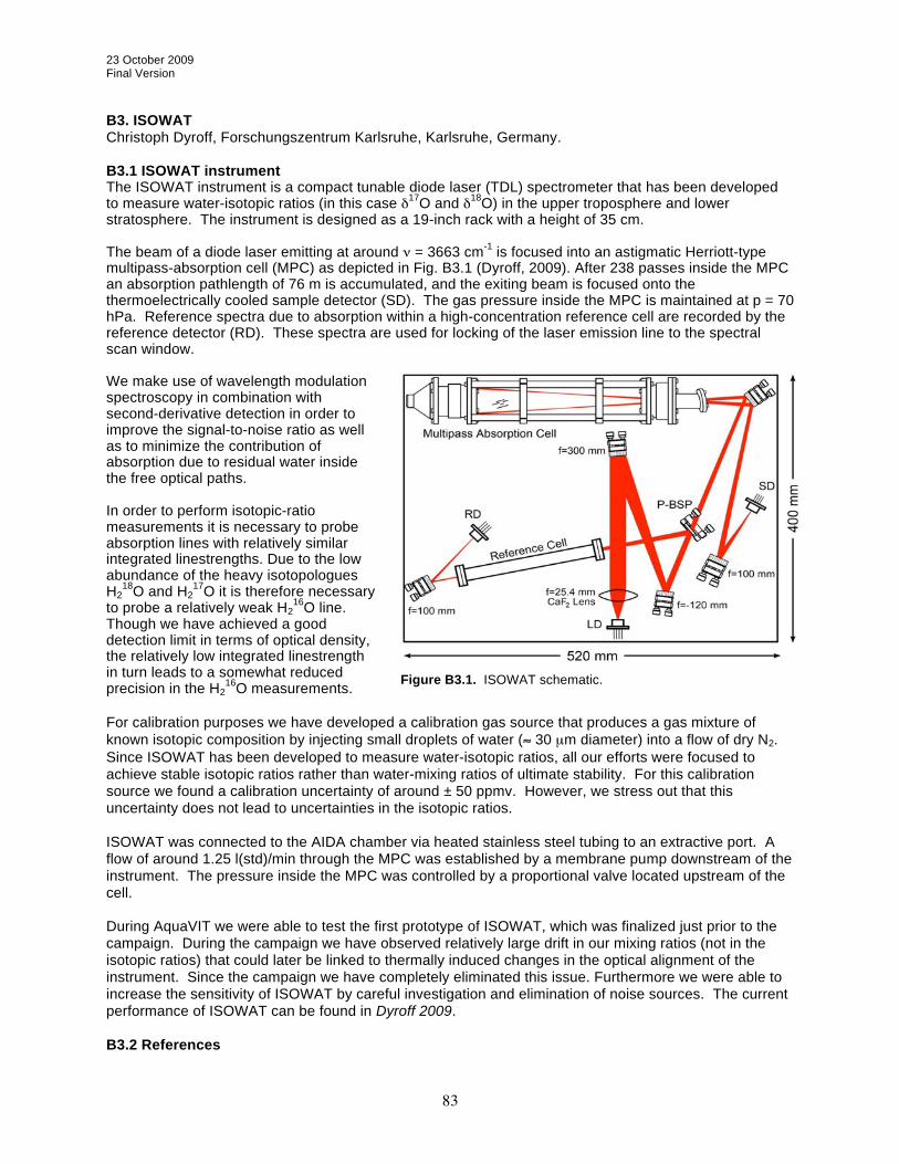
23 October 2009 Final Version
83
B3. ISOWAT Christoph Dyroff, Forschungszentrum Karlsruhe, Karlsruhe, Germany. B3.1 ISOWAT instrument The ISOWAT instrument is a compact tunable diode laser (TDL) spectrometer that has been developed to measure water-isotopic ratios (in this case 17O and 18O) in the upper troposphere and lower stratosphere. The instrument is designed as a 19-inch rack with a height of 35 cm. The beam of a diode laser emitting at around = 3663 cm-1 is focused into an astigmatic Herriott-type multipass-absorption cell (MPC) as depicted in Fig. B3.1 (Dyroff, 2009). After 238 passes inside the MPC an absorption pathlength of 76 m is accumulated, and the exiting beam is focused onto the thermoelectrically cooled sample detector (SD). The gas pressure inside the MPC is maintained at p = 70 hPa. Reference spectra due to absorption within a high-concentration reference cell are recorded by the reference detector (RD). These spectra are used for locking of the laser emission line to the spectral scan window. We make use of wavelength modulation spectroscopy in combination with second-derivative detection in order to improve the signal-to-noise ratio as well as to minimize the contribution of absorption due to residual water inside the free optical paths. In order to perform isotopic-ratio measurements it is necessary to probe absorption lines with relatively similar integrated linestrengths. Due to the low abundance of the heavy isotopologues H2
18O and H217O it is therefore necessary
to probe a relatively weak H216O line.
Though we have achieved a good detection limit in terms of optical density, the relatively low integrated linestrength in turn leads to a somewhat reduced precision in the H2
16O measurements. For calibration purposes we have developed a calibration gas source that produces a gas mixture of known isotopic composition by injecting small droplets of water ( 30 μm diameter) into a flow of dry N2. Since ISOWAT has been developed to measure water-isotopic ratios, all our efforts were focused to achieve stable isotopic ratios rather than water-mixing ratios of ultimate stability. For this calibration source we found a calibration uncertainty of around ± 50 ppmv. However, we stress out that this uncertainty does not lead to uncertainties in the isotopic ratios. ISOWAT was connected to the AIDA chamber via heated stainless steel tubing to an extractive port. A flow of around 1.25 l(std)/min through the MPC was established by a membrane pump downstream of the instrument. The pressure inside the MPC was controlled by a proportional valve located upstream of the cell. During AquaVIT we were able to test the first prototype of ISOWAT, which was finalized just prior to the campaign. During the campaign we have observed relatively large drift in our mixing ratios (not in the isotopic ratios) that could later be linked to thermally induced changes in the optical alignment of the instrument. Since the campaign we have completely eliminated this issue. Furthermore we were able to increase the sensitivity of ISOWAT by careful investigation and elimination of noise sources. The current performance of ISOWAT can be found in Dyroff 2009. B3.2 References
Figure B3.1. ISOWAT schematic.

23 October 2009 Final Version
84
Dyroff, C., Tunable diode-laser absorption spectroscopy for trace-gas measurements with high sensitivity and low drift, Ph.D. Thesis, University of Karlsruhe, 2009. ISBN: 978-3-86644-328-0, url: http://digbib.ubka.uni-karlsruhe.de/volltexte/1000010030

23 October 2009 Final Version
85
B4. OJSTER Cornelius Schiller, Martina Krämer, Armin Afchine, Reimar Bauer, Jessica Meyer, Nicole Spelten, Andres Thiel, Miriam Kübbeler, Forschungszentrum Jülich, Jülich, Germany. B4.1 Instrument description OJSTER (Open-path Jülich Stratospheric TDL Experiment) is an open path cell diode laser experiment manufactured by MayComm Inc., California. The open path Herriot multipath cell allows for absorption lengths of 4 m. The 1.37 m diode laser can be tuned over a H2O absorption line, and analysed both in direct absorption or the 2f mode. The instrument is similar to the ER-2 instrument described in May [1998], as well as the matrix method to compensate for pressure and temperature dependence. This calibration matrix is provided by the manufacturer carried out in a climate chamber against an Edgetech Dewprime 2000 Chilled Mirror system. This calibration has been re-evaluated in the Juelich laboratories against the MBW-30 frost point hygrometer which also serves as reference hygrometer for FISH calibrations. First aircraft measurements and characterisation of OJSTER in the laboratory are given in Schlicht [2006]. B4.2 Performance during AquaVIT During AquaVIT, the open-path cell of OJSTER was mounted in a stainless-steel container with a volume of a few litres in the cold space of AIDA. AIDA air was sucked by a pump via stainless-steel tubes. This experimental setup had two major disadvantages: First, the outgassing of the OJSTER cell components was very slow, even after several cycles of purging with dry warm air a background H2O contamination of the order of 20 ppmv was detected. Secondly, the container leaked at lowest temperatures, therefore no measurements at all were obtained on AquaVIT days with lowest temperatures. OJSTER data during AquaVIT therefore cannot be used for a quantitative comparison with other hygrometers. B4.3 Reference May, R., Open-path, Near-infrared tunable diode laser spectrometer for atmospheric measurements of
H2O, J. Geophys. Res., D15, 103 (1998). Schlicht, Untersuchungen zur Wasserpartitionierung in Wolken (in German), Ph.D. thesis U. Aachen,
2006.

23 October 2009 Final Version
86
B5. PicoSDLA
Georges Durry, CNRS - Groupe de Spectrométrie Moléculaire et Atmosphérique (GSMA) and University of Reims, France. PicoSDLA is a tunable diode laser spectrometer that measures in situ H2O by absorption spectroscopy at 2.63 micron. The beam emitted by an antimonide laser diode is propagated in the open atmosphere over a 1-m distance and in situ spectra are recorded with an InAs detector at 1s intervals. The sensor is to be operated from stratospheric balloons. At the time of the Aquavit experiment, the PicoSDLA was still under development and it had just been tested on flight three months before the beginning of the campaign. For a detailed description of the laser hygrometer see [Durry et al., 2008]. For the calculation of the water vapor mixing ratios, a non linear least-square fit was applied to the full molecular line shape using a molecular model based on the Beer-Lamber law in conjunction with P and T measurements yielded by onboard sensors. Detection technique is a standard direct-differential method. With all the sources of errors taken into account (baseline determination, spectroscopy, nonlinearities in the laser spectral emission, achieved signal to noise ratio in the spectra, uncertainties in P and T determination …), the expected precision error in the water vapor mixing retrieval ratios range between 5 to 10 percent in UT-LS conditions. PicoSDLA was installed outside the AIDA chamber but inside the chamber thermal structure. The laser hygrometer was implemented into a 120 mm-diameter cylinder with a length of 1m50. This cylinder was located at the bottom of the AIDA chamber. The inlet of the chamber was connected to the cylinder with a flexible connection (Tombac, DN40mm). The output of the cylinder was connected to a vacuum pump and to a flow rate regulator. Electric wires were passed through special vacuum connector capable of operations at very low temperatures (down to -90°C).The flow rate was adjusted during the calibration campaign with a regulator in the control room of Aquavit. This regulator was set between 10 to 30 l/min (at very low pressure, the real flow rate was less than 10 l/min). During AquaVIT, typical flow rates through the instrument were of 1.0 SLM decreasing to about 0.3 SLM at a total AIDA pressure of 100 hPa. At lower pressures, the small flowrates lead to a very slow effective time response of the instrument. Once installed in the cylinder, the PicoSDLA was operated continuously with no intervention on the sensor during the full campaign. The behavior of the laser hygrometer installed in the cylinder was really satisfying in terms of laser stability and quality of the absorption spectra despite the low temperature encountered (down to -90°C) and the duration of the measurement (10 days, 8 hours per day, to compare with the three hours of duration of a standard stratospheric flight). Actually our instrument is not designed for operation in a close cell like in the present configuration. It is operated open to the atmosphere from a stratospheric balloon. It means that the air sample between laser and detector is renewed every second (descent speed of the balloon at 2/3 m/s with a cell length of 1m). The equivalent flow rate would be of more than 30 SLM. The effect seen during this calibration is that, for medium H2O concentration and with a sufficient flow rate, PicoSDLA gives good result in agreement with the reference data (see discussions in previous chapters). Nevertheless, one critical issue for PicoSDLA in the present configuration, is the contamination by water vapor outgassing from the instrument itself or from the cylinder envelope; this effect could even be enhanced by the fact that we use flat heaters at different places in the instrument to maintain proper operation of the laser, detector and electronics. It could explain for the disagreement observed at very low water vapor concentration with reference data. Retrospectively, by looking at the yielded data, it would have been perhaps more appropriate to locate the laser sensor in the main chamber with the core instruments. The relation between flow rate, heaters operations and potential H2O outgassing effect in the cylinder, is still unclear to us. B5.1 References

23 October 2009 Final Version
87
G. Durry, N. Amarouche, L. Joly, X. Liu, V. Zéninari and B. Parvitte, “Laser diode spectroscopy of H2O at 2.63 micron for atmospheric applications”, Applied Physics B, 90, 573–580, 2008.

23 October 2009 Final Version
88
B6. WaSul-Hydro2 Zoltan Bozóki, Árpád Mohhácsi, University of Szeged, Hilase Ltd., Szeged, Hungary. During the campaign WaSul-Hygro was operated fully automatically without being supervised by the Hungarian group. It is only after the campaign, during data evaluation it became clear that WaSul-Hygro1 and WaSul-Hygro2 instruments were almost always operated under overload conditions caused by excessive acoustical noises inside the gas handling system, which ruined most of the measured data. Based on this experience the WaSul-Hygro instruments are now equipped with additional acoustic buffer volumes, and there is also an overload detection algorithm implemented into its electronics.

23 October 2009 Final Version
89
B7. AIDA PCI extractive TDL (APeT) Volker Ebert, Christian Lauer, Stefan Hunsmann, Harald Saathoff, Steve Wagner University of Heidelberg and Forschungszentrum Karlsruhe, Germany. The AIDA PCI extractive TDL (APeT) spectrometer aims at measuring the total water contents (vapor, ice, liquid water) in the AIDA chamber by extracting a gas sample, completely evaporating all condensed water species and then measuring the resulting vapor phase water with a very similar setup then the APicT instrument. APeT therefore uses the identical measurement principle as the APicT and no changes with regard to the software were necessary. The large majority of the hardware is also completely identical to the APicT instruments, especially the electronics, data acquisition and the laser and detectors is the same. The only changes concern the measurement vessel Figure A7.1 shows the schematic setup of the APeT. It consists of an outer vacuum recipient made of stainless steel, which is 20 cm in inner diameter and 85 cm in length. This recipient contains the fiber-coupled transfer optics and the actual measurement cell, a commercial multipath cell of Herriott type. Parasitic absorption generated by ambient air contamination is minimized, since the entire open optical path lies inside the vacuum recipient. The optical path consists of a folded (74 passes) path of 29.9 m inside the Herriott cell and additional 0.4 m between the Herriott cell and the optical components. This yields a total optical path length of 30.3 m.
Figure B7.1. Schematic of the APeT instrument. Block arrows indicate the path of the measurement gas. First, the measurement gas is conducted directly into the central Herriott cell (gray shaded) through stainless steel tubes. A baratron (P) measures the gas pressure just before entering the APeT, while a thermocouple (T) measures the gas temperature as close as possible to the Herriott cell. After leaving the Herriott cell, the gas purges the enclosing vacuum recipient, which also contains the transfer optics. The optics consists of a fiber-coupled collimator (C) and a photodiode detector (D). Light from the collimator couples into the Herriott cell and falls onto the detector after coupling out of the Herriott cell. This yields a total optical path length of 30.3 m, of which 29.9 m are inside the Herriott cell and 0.4 m in the vacuum recipient.
Gas pressure is determined by a baratron with a range of 0-1333 mbar and gas temperature by a thermocouple of type K. The measurement gas is directly conducted into the Herriott cell after entering the APeT and subsequently purges the outer vacuum recipient before leaving the APeT. This ensures that the entire gas flow is used to purge the Herriott cell resulting in a minimal gas exchange time within the cell, while purging of the outer vacuum recipient is also maintained. The volume flow rate of the measurement gas is approximately 9 l/min independent of its pressure. The volume of the Herriott cell is 0.9 l, while the effective volume of the vacuum recipient is approximately 25 l. Thus, 99.7% of the gas volume inside the Herriott cell is exchanged in 18 s. For the vacuum recipient this takes approximately 8 min. Since 99% of the optical path lies inside the Herriott cell, this does not affect the measurement result significantly. The APeT achieves a resolution (1s) of 25 ppb water vapor mixing ratio with a dynamic range from below 1 ppm to above 1000 ppm. APeT has been developed for the Aquavit campaign and was used mostly for the second week. The data in the first week were not suitable due to leak problems.

23 October 2009 Final Version
90
B8. Closed-path Laser Hygrometer (CLH) Linnea Avallone, Sean Davis, University of Colorado, Boulder, CO, USA. B8.1 CLH material for AquaVIT white paper The University of Colorado Closed-path Laser Hygrometer (CLH) is a tunable diode laser spectrometer originally built by R. D. May of SpectraSensors, Inc., and modified for cloud particle observations at the University of Colorado. This sensor is virtually identical, except for its internal absorption cell and inlet, to open-path instruments (designated JLH) flown by the JPL group (May and Herman) on the NASA ER-2, DC-8, and WB-57F aircraft. These water vapor spectrometers use near-infrared (1.37 μm) tunable diode laser (TDL) sources that provide reliable single-mode output power in the 5-25 mW range. In addition to their small size and dependability, these lasers are attractive because they operate near room temperature, eliminating the need for dewars and cryogens. Instead, thermoelectric elements (often called TE coolers) are used to stabilize the temperature of the laser to about 15 oC. The laser wavelength is scanned over the absorption line and modulated at high frequency by varying the diode injection current. Both direct and second-harmonic (2f) absorption spectra are recorded by the CLH, and the water vapor mixing ratio is calculated using the 2f line strength (for details see Davis et al., 2007a). The CLH has been coupled to specially designed sub-isokinetic inlets for use on aircraft. These inlets take advantage of the particulate enhancement from the sub-isokinetic flow to achieve substantial signal-to-noise ratios in the total water measurement, which is particularly useful for measuring the ice water content in thin clouds. Additional instrument details, as well as information about accuracy and precision, are provided in Davis et al., 2007a,b. During AquaVIT, the CLH was used in extractive mode, drawing air from the AIDA chamber at flow rates ranging from 0.75 - 10 SLM. The instrument was used without its flight inlet and was coupled to the chamber by heated stainless steel tubing. The flow path within the instrument was heated to 40 oC, as in flight. Data were obtained at a rate of 7.8 Hz (8 128-msec scans per second) and averaged to produce water vapor mixing ratios every second. B8.2 Performance in the static experiments The CLH instrument provided only limited data during the static experiments because of two technical problems; both of these were addressed for the dynamic experiments. First, a break in a weld attaching the pressure port to the absorption cell led to a small leak. Due to the nature of the extractive sampling at AquaVIT (absorption cell at low pressure with the rest of instrument at high pressure), the cell was contaminated by ambient water vapor entering through the pinhole leak. This leak would probably have gone unnoticed under flight conditions, because the instrument is constructed to fly in an unpressurized environment with little differential pressure between the absorption cell and its surroundings. The impact of the leak was minimized by sealing it as well as possible using vacuum sealant and by maintaining a high flow rate through the instrument. Measurements made at fixed mixing ratio and variable flow rate showed that this strategy was, for the most part, successful. Data for chamber pressures at which inadequate flow through the instrument was achieved were not submitted for comparison. Prior to AquaVIT some instrument electronics were changed to allow for sampling at ~8 Hz (rather than the previous rate of 0.65 Hz). An improper gain setting on a new computer board led to incorrect recording of the 2f laser modulation amplitude, which resulted in undermodulation and subsequent overestimation of water vapor amounts. The true laser modulation amplitude was obtained through a series of measurements made at fixed mixing ratio and was confirmed with laboratory etalon measurements. The AquaVIT data were then reprocessed using the correct modulation value. However, undermodulation of the laser resulted in a reduction of the CLH precision and increase in the detection limit by about a factor of two during AquaVIT as compared to normal operating conditions. Finally, the nature of the instrument itself limited its application under many of the AquaVIT conditions. The absorption path is fairly short (27.6 cm) because it is optimized for cloud water detection rather than for measurement of ambient water vapor in the upper troposphere and lower stratosphere. As a result, the water vapor detection limit is about 10-20 ppm, depending on pressure and laser modulation amplitude. Thus, the AIDA mixing ratios were often below the operational range of the instrument. B8.3 References

23 October 2009 Final Version
91
S. M. Davis, A. G. Hallar, L. M. Avallone, and W. Engblom, 2007a, Measurements of ice water content with a tunable diode laser hygrometer: Calibration procedure and inlet analysis, J. Atmos. Oceanic Technol., 24, 463, doi:10.1175/JTECH1975.1.
S. M. Davis, L. M. Avallone, E. M. Weinstock, C. H. Twohy, J. B. Smith, and G. L. Kok, 2007b, Comparisons of in situ measurements of cirrus cloud ice water content, J. Geophys. Res., 112, D10212, doi:10.1029/2006JD008214.

23 October 2009 Final Version
92
B9. VCSEL Hygrometer Mark A. Zondlo,1 Mark E. Paige,2 and Joel A. Silver2
1-Dept. of Civil and Environmental Engineering, Princeton University, Princeton, NJ 87505 2-Southwest Sciences, Inc., Santa Fe, NM 87505 B9.1 Introduction The NSF G-V VCSEL hygrometer is a new instrument that is being flown on the NSF Gulfstream-V research aircraft. While the instrument was still in its development stage at the time of the campaign, the Aqua-VIT program served as a test and validation of a unique calibration method for conditions representative of the upper troposphere and lower stratosphere as well as the first intercomparisons with other research grade sensors at low mixing ratios. On the day before the campaign, there was a catastrophic event that destroyed the laser diode drive current and destroyed the laser. The laser and circuit were repaired by the last day of the static experiments, but significant outgassing of the sampling lines prevented reliable data from being acquired. No data was submitted for the static experiments, though blind data was submitted for the dynamic experiments (second week). Details of the performance in Aqua-VIT, calibrations of the sensor, and intercomparisons with the German PTB source are described.
B9.2 Experimental B9.2.1 VCSEL hygrometer configuration during Aqua-VIT To interface with the AIDA chamber most efficiently, the VCSEL hygrometer configuration during Aqua-VIT differed somewhat from the final, aircraft design. The aircraft version of the sensor, shown in Fig. 1, consists of a pylon that resides outside the fuselage and an electronics box immediately below it inside the cabin. A pair of gold-coated, 1.91 cm diameter copper mirrors is separated by 14.95 cm in the pylon and a thermistor and static pressure probe measure local conditions about 1 cm behind the optical path. Infrared light around 1854 nm is end-coupled from the VCSEL inside the electronics box into a fiber optic (9 m core/125 m cladding, l=50 cm) which terminates in the lower mirror with a gradient index lens. Light passes 25 times in the Herriott cell and is focused onto an extended wavelength InGaAs detector by a narrow (7.5 half angle) lens in the upper mirror. Because the instrument was still in its development stages during Aqua-VIT, it was decided to keep the entire sensor outside the cloud chamber in order to conduct routine maintenance in an efficient manner. The use of a heated sampling line at 298 K resulted in a loss of sensitivity under UT/LS conditions relative to the aircraft version due to the temperature dependence of the 1854.03 nm absorption line. For example, the absorbance of this peak at 5 ppmv H2O at 135 hPa and 210 K is 4.0 10-3 but this decreases to 2.4 10-3 at 303 K. To connect to the heated line from the AIDA chamber in the most efficient manner, the optical cell was intented to be replicated with the same pathlength and configuration inside an ultra-high vacuum housing. Unfortunately, due to fabrication errors with the mirror focal lengths, the Herriott pattern instead was a 15-pass system with a 2.2 m total pathlength. The same fiber optic feedthrough, temperature sensor, and pressure feedthrough were used as in the aircraft version. The housing was sealed by copper gaskets for all fittings except the fiber optic feedthrough which was a ” NPT thread. A 1 m patch cable for the fiber optic was added between the laser and the fiber optic feedthrough. All other aspects of the sensor remained identical to the aircraft version. Due to a laser failure and driver circuit problem, no data were collected during the first four days of the static intercomparison (Experiments 3-7). A new laser from Vertilas was installed and characterized to first order in the field. Data were collected for the final day of the static tests at nominal 0.5-5 ppmv levels, but outgassing water vapor caused a significant and unquantified background, and no data were submitted to the archive for Experiment 8. In addition, large étalons were observed from the fiber optic feedthrough after the laser replacement, and the étalons prevented efficient linelocking for Experiments 9
Figure B9.1. Photograph of the NSF G-V VCSEL hygrometer showing the pylon (blue) and electronics box (red). The gold-colored plate is the surface of the fuselage.
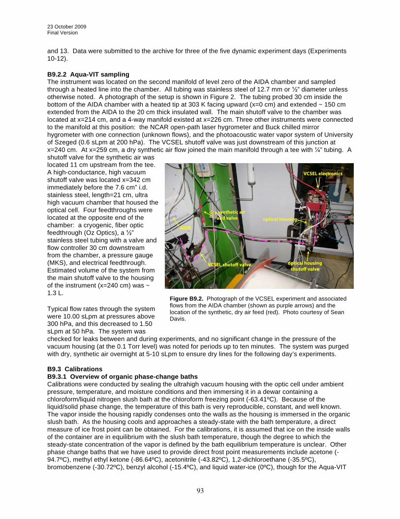
23 October 2009 Final Version
93
and 13. Data were submitted to the archive for three of the five dynamic experiment days (Experiments 10-12). B9.2.2 Aqua-VIT sampling The instrument was located on the second manifold of level zero of the AIDA chamber and sampled through a heated line into the chamber. All tubing was stainless steel of 12.7 mm or ” diameter unless otherwise noted. A photograph of the setup is shown in Figure 2. The tubing probed 30 cm inside the bottom of the AIDA chamber with a heated tip at 303 K facing upward (x=0 cm) and extended ~ 150 cm extended from the AIDA to the 20 cm thick insulated wall. The main shutoff valve to the chamber was located at x=214 cm, and a 4-way manifold existed at x=226 cm. Three other instruments were connected to the manifold at this position: the NCAR open-path laser hygrometer and Buck chilled mirror hygrometer with one connection (unknown flows), and the photoacoustic water vapor system of University of Szeged (0.6 sLpm at 200 hPa). The VCSEL shutoff valve was just downstream of this junction at x=240 cm. At x=259 cm, a dry synthetic air flow joined the main manifold through a tee with ” tubing. A shutoff valve for the synthetic air was located 11 cm upstream from the tee. A high-conductance, high vacuum shutoff valve was located x=342 cm immediately before the 7.6 cm” i.d. stainless steel, length=21 cm, ultra high vacuum chamber that housed the optical cell. Four feedthroughs were located at the opposite end of the chamber: a cryogenic, fiber optic feedthrough (Oz Optics), a ” stainless steel tubing with a valve and flow controller 30 cm downstream from the chamber, a pressure gauge (MKS), and electrical feedthrough. Estimated volume of the system from the main shutoff valve to the housing of the instrument (x=240 cm) was ~ 1.3 L. Typical flow rates through the system were 10.00 sLpm at pressures above 300 hPa, and this decreased to 1.50 sLpm at 50 hPa. The system was checked for leaks between and during experiments, and no significant change in the pressure of the vacuum housing (at the 0.1 Torr level) was noted for periods up to ten minutes. The system was purged with dry, synthetic air overnight at 5-10 sLpm to ensure dry lines for the following day’s experiments. B9.3 Calibrations B9.3.1 Overview of organic phase-change baths Calibrations were conducted by sealing the ultrahigh vacuum housing with the optic cell under ambient pressure, temperature, and moisture conditions and then immersing it in a dewar containing a chloroform/liquid nitrogen slush bath at the chloroform freezing point (-63.41ºC). Because of the liquid/solid phase change, the temperature of this bath is very reproducible, constant, and well known. The vapor inside the housing rapidly condenses onto the walls as the housing is immersed in the organic slush bath. As the housing cools and approaches a steady-state with the bath temperature, a direct measure of ice frost point can be obtained. For the calibrations, it is assumed that ice on the inside walls of the container are in equilibrium with the slush bath temperature, though the degree to which the steady-state concentration of the vapor is defined by the bath equilibrium temperature is unclear. Other phase change baths that we have used to provide direct frost point measurements include acetone (-94.7ºC), methyl ethyl ketone (-86.64ºC), acetonitrile (-43.82ºC), 1,2-dichloroethane (-35.5ºC), bromobenzene (-30.72ºC), benzyl alcohol (-15.4ºC), and liquid water-ice (0ºC), though for the Aqua-VIT
Figure B9.2. Photograph of the VCSEL experiment and associated flows from the AIDA chamber (shown as purple arrows) and the location of the synthetic, dry air feed (red). Photo courtesy of Sean Davis.

23 October 2009 Final Version
94
results only chloroform was used. The small size of the optical cell and instrument certainly facilitate these types of calibrations. Advantages of this approach include the reproducibility, stability, and accuracy of the bath temperature (other slush bath temperatures exist, of course, too). In addition, one can pump out the cell to calibrate under different pressure conditions. In this way, the sensor is being calibrated under representative temperature, pressure, and humidity of the upper troposphere and lower stratosphere. Biases from adsorption to tubing surfaces or residual water in nitrogen flows (e.g. in standard dilution) are not an issue in these static calibrations, and the walls rapidly equilibrate with the surrounding bath. The water vapor is in steady-state with the ice on inside walls of the housing. For the Aqua-VIT housing, the inner diameter of the housing was only a radius of 3.8 cm, so the timescale from diffusion alone is on the order of minutes. Caveats of this approach include the requirement for the inside walls of the container to fully reach thermal equilibrium with the slush bath temperature, the need for surfaces to be fully immersed in the bath (though warm spots should eventually vapor transfer to the coldest temperature spots), and necessity for a well-mixed phase change bath. The thermal time to reach equilibrium is probably the largest source of uncertainty. Indeed, for the Aqua-VIT results, it appears that the system did not fully reach equilibrium, and this likely caused the high bias for our results. B9.3.2 Details of the chloroform bath calibration A chloroform bath calibration was conducted at the start and finish of the campaign, but with a new laser and associated tuning parameters, only the final calibration was used. The chloroform bath was made with > 99.0-99.4% purity, ACS reagent grade chloroform (Merck KGaA) mixed with liquid nitrogen. The bath was stirred on occasion to break up the largest pieces into a fine slush. This bath was made in a stainless steel, vacuum tight dewar with dimensions of 45 cm height and 25 cm inner diameter. The slush bath maintained two phases of chloroform for over twelve hours when left undisturbed, though over this timescale the solid particles sunk to the bottom. A thin layer of chloroform ice formed on top with the addition of liquid nitrogen every 10-30 minutes, and this layer was broken and stirred to ensure a well-mixed bath. Visually, the bath maintained a consistent mixture of fine slush throughout the calibration. In this way, an isothermal bath was maintained. The bath covered the entire calibration cell except for the uppermost feedthroughs. It took about two hours for the air temperature thermistor inside the center of the vessel to reach a stable value on the timescales of the experiments (+/- 0.5 K). This value was ~ 2.5 K higher than the value when the same thermistor was placed inside the bath directly. Residual heating from the mirror heaters were likely the source of the warmer air temperature. During the time to reach steady-state, the absolute concentration of water vapor was measured. Figure 3 shows a plot of the reported number density (red) versus time as the housing was immersed in the baths. Also shown on the right is the pressure measurement. Initially, as the temperature dropped, so does the pressure due to the ideal gas law. At t=2000 s, ambient air was added to the bath to raise the pressure. The introduction of ambient air initially raised the concentration of water vapor, but it very quickly returned
Figure B9.3. Results of the chloroform slush-bath immerision calibration. The red line shows the raw (uncorrected) water vapor concentration in molec cm-3. The blue line shows the pressure.

23 October 2009 Final Version
95
to the previous level within a few minutes. The timescale for diffusion of water vapor in nitrogen at these temperatures and pressures ranged from one to five minutes using a scale length of the calibration cell, and this was in excellent agreement with the experimental data which showed a rapid loss of ambient water vapor to concentrations defined by the ice bath temperature within a few minutes. At t=6500 s, the pressure was changed in the cell stepwise from 500 hPa to 80 hPa every 500 s intervals. If the vapor was truly in equilibrium with the ice at the bath temperature, the concentration should not change with time. Indeed, very little deviation is noted in the concentration during the pressure changes except at the very onset. The adiabatic expansion of pumping the calibration cell induced a slight decrease in water vapor concentration as it took time for the ice vapor pressure to re-establish equilibrium in the vapor phase. Data from the last minute of each pressure step were averaged before the pressure was adjusted again. Changes in the reported concentration as a function of pressure were minimal (<1%) for the results from 76 to 510 hPa. The raw concentration data from the new laser was then scaled by 0.442 based upon this calibration and used as a benchmark for all data from AquaVIT. After further studies since the Aqua-VIT campaign, it appears that the data in Fig. 3 likely did not fully reach steady-state when the pressure calibrations were conducted. Based upon subsequent studies beyond the final data submission, it appears that it is necessary to wait about 1000 s for each pressure step to reach steady-state. For this case, calibrating at slightly less values than “equilibrium” would result in a slight (<10%) adjustment downward of our final data, though it is unclear by the exact amount. Overall, the organic slush method shows much promise for calibrations at UT/LS conditions, though care must be taken to ensure a steady-state near equilibrium is achieved. Calibrations for the Aqua-VIT data did not appear to fully reach equilibrium, but we note that this was the first time such a calibration had been conducted with this instrument. B9.4 Intercomparisons The VCSEL sensor was also intercompared with the German PTB standard at the end of the campaign. The PTB standard was moved to a location 4 m away from the VCSEL hygrometer twenty-four hours prior to the measurement, and the temperature setpoint was adjusted to emit at a mixing ratio of 14.76 ppmv at 1.00 sLpm. The VCSEL was intercompared to the PTB standard over three flows (1.00 sLpm, 3.00 sLpm, and 9.00 sLpm) corresponding to three different mixing ratios (14.76, 4.92, and 1.62 ppmv, respectively). The first flow of 1.00 sLpm was maintained for two hours prior to the experiments, but subsequent flow (mixing ratio) changes had much shorter periods before measurement due to time constraints (25 min. at 3.00 sLpm before beginning measurements; 2 min. at 9.00 sLpm). The intercomparison was conducted at four pressure ranges to help examine the instrument performance as a function of pressure. Figure 4 shows the response of the VCSEL mixing ratio as a function of the pressure changes for the 14.76 ppmv, 4.92 ppmv, and 1.62 ppmv levels. The highest two mixing ratios were examined at ~ 80, 191, 298, and 508 hPa. For the lowest mixing ratio, because of the étalons in the fiber optic feedthrough, decreased optical pathlength, and lower cross sections at 303 K sampling condtions relative to atmospheric temperatures, the signal-to-noise ratio was poor. The sensor was kept
Figure B9.4. Time series for the VCSEL for three different flows (mixing ratios) from the PTB standard (dashed, black line). The pressures were varied from 76 to 510 hPa for the nominal 4.92 and 14.76 ppmv concentrations. Reliable signal was only obtained at 200 hPa for the 9 sLpm flow (start and end).

23 October 2009 Final Version
96
at 200 hPa at 1.62 ppmv for a short duration only at the start and end as it appeared to be only just above the signal-to-noise limit at the time of the experiment. Pressure was adjusted by manually adjusting the pumping speed downstream of our optical cell housing to achieve the desired pressure level but keeping the incoming flow from the PTB source constant. Averaged over all the pressure ranges, our measurements were 14.4 ± 0.8 ppmv for the PTB calculated value of 14.76 ppmv (1.00 sLpm), 4.81 ± 0.70 ppmv for the PTB value of 4.92 ppmv (3.00 sLpm), and 1.49 ± 0.5 ppmv for the PTB standard of 1.64 ppmv (9.00 sLpm). Figure 5 shows a plot of the VCSEL data versus PTB at different pressures. Within a constant flow rate, the higher pressures had higher mean mixing ratios relative to the lower pressure data. This may be related to not waiting enough time for the tubing walls to equilibrate to the new flow rate at the first (and lowest) pressures within a given mixing ratio. Alternatively, it could be due to imperfect characterization of the laser over the range of pressures. Given the noise in our data from the étalon, a non-optimally characterized laser, and the first attempt at using slush baths for calibrations, it is encouraging that we agree within error bars with the German PTB mixing ratios. This also helps verify that the slush bath method of calibration does not suffer from large systematic biases. Further work on the calibration of the instrument is currently ongoing with more temperature baths and more accurate spectroscopic parameters.
Figure B9.5. Plot of the VCSEL vs. PTB over the range of conditions studied (colored by pressure).
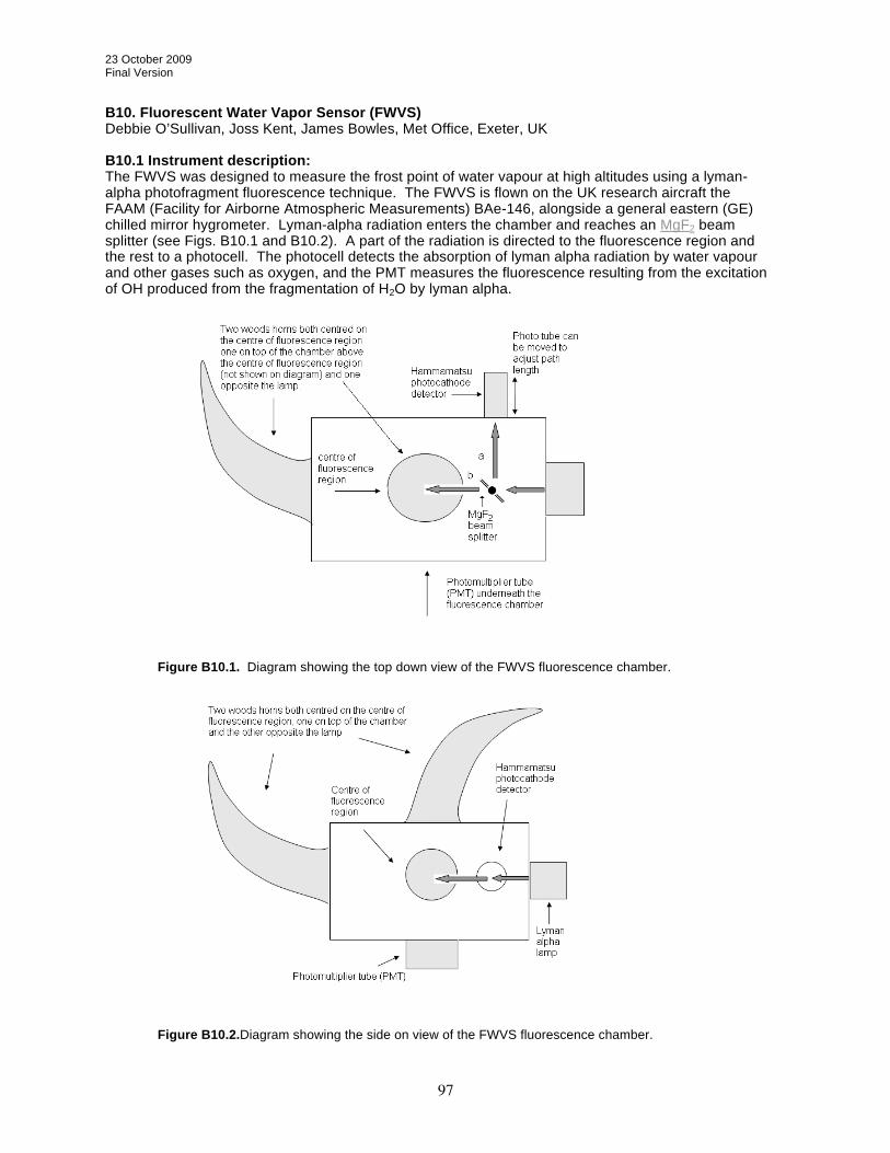
23 October 2009 Final Version
97
B10. Fluorescent Water Vapor Sensor (FWVS) Debbie O’Sullivan, Joss Kent, James Bowles, Met Office, Exeter, UK
B10.1 Instrument description: The FWVS was designed to measure the frost point of water vapour at high altitudes using a lyman-alpha photofragment fluorescence technique. The FWVS is flown on the UK research aircraft the FAAM (Facility for Airborne Atmospheric Measurements) BAe-146, alongside a general eastern (GE) chilled mirror hygrometer. Lyman-alpha radiation enters the chamber and reaches an MgF2 beam splitter (see Figs. B10.1 and B10.2). A part of the radiation is directed to the fluorescence region and the rest to a photocell. The photocell detects the absorption of lyman alpha radiation by water vapour and other gases such as oxygen, and the PMT measures the fluorescence resulting from the excitation of OH produced from the fragmentation of H2O by lyman alpha.
Figure B10.1. Diagram showing the top down view of the FWVS fluorescence chamber.
Figure B10.2.Diagram showing the side on view of the FWVS fluorescence chamber.

23 October 2009 Final Version
98
B10.2 Principle of a Lyman-alpha hygrometer – Absorption mode:
Lyman-alpha radiation is emitted by hydrogen atoms at a narrow line in the far ultraviolet portion of the spectrum (121.56 nm). It is produced by an electrical discharge in hydrogen. As the Lyman-alpha radiation passes across the sensing chamber, it is partially absorbed by atmospheric water vapour H2O + hv ( 121.56 - 137 nm) OH*( 2 +) + H(2S) absorption (1) thus decreasing the detected signal (I). This signal change follows the Beer-Lambert law such that:
I = I0 exp (- xp/p0) (2) where: I = received signal I0 = intensity of the lamp
= absorption cross section for water vapour at lyman-alpha at STP x = path length; p = concentration of water vapour in the sensing volume; p0 = concentration of water vapour at STP If I0 is known and if water vapour is the only gas to absorb lyman-alpha and therefore attenuate the signal then the received signal, I will be directly proportional to the water vapour content within the sample volume. However in practice, liquid water, oxygen, and ozone will also absorb significant amounts of Lyman-alpha radiation and thus attenuate the received signal. This needs to be accounted for as part of the calibration procedure. In addition the refractive index of the beam splitter needs to be accounted for. B10.3 Principle of a Lyman-alpha hygrometer – Fluorescence mode: When a molecule of water vapour absorbs radiation with a wavelength of less than 137 nm, such as Lyman alpha, the water molecule photodissociates to OH and H. A proportion of the resulting OH is in the electronically excited OH( 2 +) state. The proportion of any given state produced is given by the quantum yield . In reaction (3) the quantum yield for OH production is 1, however the quantum yield for the production of OH in the ( 2 +) excited state is a maximum of 0.1 (Wu et al., 1992; Yi et al., 2007).
H2O + hv ( 121.56 - 137 nm) OH*( 2 +) + H(2S) absorption (3)
The excited OH can then undergo radiative relaxation to the ground state OH(X2 ), releasing a photon with a wavelength of around 310 nm. This is the fluorescence which is measured by the photomultiplier (PMT).
OH*( 2 +) OH(X2 ) + hv ( 310 nm) (4) Not all of the OH( 2 +) will undergo radiative relaxation, some will be “quenched” by collisions with other molecules mainly N2 and O2 collectively denoted as M. (This process is pressure dependent, with quenching rates increasing with higher pressures). OH*( 2 +) + M products (5) In the theory currently being used to interpret the FWVS data the mechanism put forward by Kley and Stone (1978) is used. As such the production of OH*( 2 +) required for fluorescence is given simply by:
[OH*( 2 +)] = Is [H2O] (6) A0+k15[M]
Where: Is = the intensity of lyman alpha in the sample region
= lyman alpha absorption cross-section of water vapour, = quantum yield of OH*( 2 +) from reaction (1)
[H2O] = number density of water vapour (molecules-1 cm-2) A0 = transition probability per second of relaxation to the ground state (Einstein (A) coefficient) k15 = quenching coefficient for OH* by air [M] = number density of air
If we equate [H2O] to the volume mixing ratio of water vapour in air (μH2O) then the fluorescence measured by the photomultiplier is given by:

23 October 2009 Final Version
99
[OH*( 2 +)] A0 = F = μH2O Is A0 [M] (7) A0+[M] k15
Is can be obtained from the received Signal I and equation (2) provided that the path length I0 to I is the same as I0 to Is. [OH*] is the measured fluorescence after subtracting the background count rate, and , , A0, k15 are all constants.
In the troposphere and lower stratosphere at altitudes < ~35 km, collisional quenching of OH*( 2 +) to the ground state is much greater than radiative relaxation to the ground state [M] k15 >> A0 (Kley and Stone, 1978, Kley et al., 1979; Kley, 1984), and equation (7) can be reduced and rearranged to get:
μw = F (9) Is (k15/A0)
Everything on the bottom of equation (9) apart from Is is a constant, and so can be combined into a single constant C
μw = F (10) Is C
The calibration constant C, is then experimentally determined – this is the most problematic part of the FWVS operation and work is currently being undertaken to improve both the calibration procedure and the instrument design to reduce the uncertainties. B10.4 Calibration
Normally the FVWS is calibrated in the laboratory against a general eastern chilled mirror hygrometer and more recently using a Buck CR2 hygrometer, across a range of temperatures controlled using a water bath. The calibration constant C is obtained by plotting the measured fluorescence divided by the intensity of lyman alpha measured with the photo tube against the water vapour mixing ratio measured by the reference hygrometer. This method is however quite crude and is need of improvement. For AquaVIT the FWVS was calibrated using the Jülich FISH calibration bench to obtain a more accurate value for the calibration constant C.
B10.5 Performance of FWVS during AquaVIT FWVS was installed on the ground floor level of the AIDA chamber via a 13 mm inlet, shared with the CARIBIC CR2 frost point hygrometer, the CARIBIC Photoacoustic instrument and an isotope TDL. Data were only obtained for experiments 01 – 04, due to the very limited time available for the Met Office participation in AquaVIT. Experiments 03 (15th October) and 04 (16th October) were part of the formal intercomparison and the results from these are shown below.
Figure B10.3. Results from Experiment 03 on the 15th October
In experiment 03 on the 15th October (Figure B10.3), the water vapour mixing ratio measured by FWVS agrees reasonably well with the values measured by both of Jülich’s FISH instruments, the Harvard water

23 October 2009 Final Version
100
vapour instrument (HWV) and the JPL instrument (JLH-TDL). However the amount of water vapour measured by FWVS tended to drift downwards during each of the constant pressure levels. Since AquaVIT this has been under investigation and it appears to be a combination of wall retention effects inside the fluorescence chamber and also the Hamamatsu phototube drifts. There may also be some other electronic problems within the instrument which are currently being investigated. The observed difference in the first part of the experiment is due to the FWVS sampling dry air to dry the instrument out after accidentally sampling very moist air before the start of the experiment.
Figure B10.4. Results from Experiment 04 on the 16th October
In experiment 04 on the 16th October (Figure B10.4) the agreement between FWVS and other groups was good for the steps where the amount of water vapour was decreasing. However for the last two steps of increasing water vapour mixing ratios the FWVS overestimated the amount of water vapour present by 10 – 20 ppm. The reason for this is not yet known.
B10.6 Summary The data obtained from AquaVIT have shown that the FWVS has the potential to accurately measure water vapour (based on comparisons with other groups) and could eventually be a reliable instrument however a number of problems were also brought to light from the inter-comparison. Firstly the tendency of the instrument to drift downwards which is due to a combination of moisture retention on the walls of the chamber and to observed drift of the Hammamatsu photocathode detector currently being used. Another problem with the instrument is that there is no direct measure of the lamp intensity, and currently fluctuations in lamp output cannot be corrected for. This is problematic when trying to calibrate the instrument and also is probably partly responsible for the instrument noise. A possible solution to this problem would be to introduce a second lyman-alpha detector to directly measure the lamp output, making the instrument design of the FWVS more similar to the Jülich FISH instruments. To address these problems the instrument is currently being redesigned and rebuilt. The electronics are all being upgraded and the Hammamatsu photocathode detector will be replaced with a new detector probably an NO cell which we are currently sourcing from Resonance in Canada jointly with the Jülich group. There will also be a new electro polished silco-steel chamber to reduce moisture retention on the walls of the instrument. All plumbing will also be electropoloished and treated. A new more powerful pump is being fitted which will enable a higher flow rate which should also aid in the removal of moisture from the fluorescence chamber. Initially it is not planned to introduce a second NO detector to monitor the lyman-alpha lamp output, as lamp is excited by a precision 144MHz crystal controlled amplifier which should produce a stable lamp output, hopefully negating the need for an extra detector. However the new chamber is being designed in such a way that a second detector could be added at a later stage if it is
23 October 2009 Final Version
101
found to be necessary. As an interim step a pair of new lyman-alpha lamps are being made which will be thoroughly tested for stability and the purity of the spectral output will also be checked. In addition a new calibration bench is planned as a result of the inter-comparison. As the calibration constant acquired using the Jülich calibration bench produced better results than that obtained using our current calibration method. A new chilled mirror hygrometer (Buck CR2) has been purchased for more accurate water vapour measurements during lab calibrations, and to provide a means of intercomparison in the air. Once the instrument and calibration procedure improvements have been carried out, there are plans to take part in further inter-comparison work in order to gauge the success of the improvements. B10.7 References Kley, D., and Stone, E, J., (1978) Measurements of water vapour in the stratosphere by photodissociation
with Ly( ) (1216 A) light. Review of Scientific Instruments, 46, pp 691-697. Kley, D., Stone, E, J.,Henderson, W.R., Drummond, J.W., Harrop, W.J., Schmeltekopf, A.L., Thompson,
T.L., and Winkler, R.H. (1979) In Situ measurements of the mixing ratio of water vapour in the stratosphere. Journal of the Atmospheric Sciences 36, pp 2513-2524.
Kley, D. (1984) Ly( ) absorption cross-section of H2O and O2. Journal of Atmospheric Chemistry 2, pp 203-210.
Wu, R.C.Y., Chen, F.Z., and Judge, D.L. (1992) Velocity distributions of H and OH produced through solar photodissociation of H2O. Asteroids, Comets, Meteors 1991, pp 657-660, Lunar and Planetary Institute, Houston (available online at: http://adsabs.harvard.edu/full/1992acm..proc..657W).
Yi, W., Park, J., and Lee, J. (2007) Photodissociation dynamics of water at Lyman alpha (121.6 nm). Chemical Physics Letters, 439 (1-3), pp 46-49.

23 October 2009 Final Version
102
Appendix C. Reference instruments C1. PTB water permeation source Designed by Physikalisch Technische Bundesanstalt (PTB) W. Mackrodt (https://aquavit.icg.kfa-juelich.de/AquaVit/Instruments/PTBPermeationSource) > Based on permeation tubes purged with dried air (here synthetic air < 1 ppm water (Basi) water via hydrosorb (Messer Griesheim)) or N2 > Calibrated to German primary humidity standard. The permeation source was calibrated at the national (coloumetric) primary humidity standard of Germany over a concentration range from 0.5 to 5 ppm. The relative uncertainty of that calibration is 2% with 50% of this uncertainty resulting from the uncertainty of the flow meters, which were calibrated with 1% relative uncertainty. Thus, if the users of the permeation source use a less precise flow meter with the permeation source the uncertainty must be increased. > H2O concentration depends strongly on
- tube temperature (3rd order polynomial / -28.3612; 2.52090; -0.0728298; 0.000871368 ) - purge gas flow provided by a FZK-calibrated flow controller (FC2900, Millipore), - tube temperature is measured with a precision calibrated PT100 resistor described by a first order
polynomial (100.045; 0.394614) - for 1SLM purge gas flow the H2O volume fraction is described by a 3rd order polynomial (28.3612;
2.52090; -0.0728298; 0.000871368) - concentration range 5-50 ppm (for bath temperatures of 30°C to 60°C and a 1SLM flow of buffer
gas) > Using the full range of the flowmeter the mixture can be varied about 10x-20x, i.e. between 250ppb and 5ppm at 30°C. Flow through the permeation source is calculated according to the calibration of the mass flow controller:
Flow (SLM) = (0.969±0.014)*(Set point value) + (0.093±0.086); Since the calibration indicates a small non linearity, the measured flows for each set point (see AquaVIT website) instead of the linear fit function may be used to calculate the flow through the permeation source. Temperature of the permeation source water bath:
T(bath, °C)= ((Resistance, Ohm)-100.045)/0.394614 Volume mixing ratio of the source output as a function of bath temperature and flow:
PPMV=(-28.3612+2.52909*T-0.0728298*T^2+0.000871368*T^3)/ Flow C1.2 PTB water permeation source intercomparisons During AquaVIT the PTB permeation source was used for intercomparison with CFH, MBW-DP30, MBW-373LX, and VCSEL. Comparison of MBW373LX (1 atm, 1 SLM) with the PTB permeation source directly after the AquaVIT campaign (October 30, 2007) showed a systematic deviation of -(4.2±3.3)% for the mixing ratios applied (1.5 – 13.5 ppm). The reason for this systematic deviation to the water permeation source is not completely clear. Besides possible problems in the permeation source or the dew point mirror instrument the flow determination seems to be the largest source of uncertainty. The MBW-DP30 frost point hygrometer used as reference instrument of the FISH calibration bench was compared to the PTB source in the range of 1-7 ppmv. The deviations of the DP30 are ±2% (see also Appendix B and Meyer et al., 2009).