summer institute in statistical genetics university of ... · occurring genetic variation in the...
TRANSCRIPT

Population Genetic Data Analysis
Summer Institute in Statistical Genetics
University of Washington
July 12-14, 2017
Jerome Goudet: [email protected]
Bruce Weir: [email protected]
1

Contents
Topic Slide
Genetic Data 3Allele Frequencies 37Allelic Association 76Population Structure & Relatedness 153Association Mapping 234
Lectures on these topics by Bruce Weir will alternate with R ex-
ercises led by Jerome Goudet.
The R material is at http://www2.unil.ch/popgen/teaching/SISG17/
2
GENETIC DATA
3

Sources of Population Genetic Data
Phenotype Mendel’s peasBlood groups
Protein AllozymesAmino acid sequences
DNA Restriction sites, RFLPsLength variants: VNTRs, STRsSingle nucleotide polymorphismsSingle nucleotide variants
4

Mendel’s Data
Dominant Form Recessive Form
Seed characters5474 Round 1850 Wrinkled6022 Yellow 2001 Green
Plant characters705 Grey-brown 224 White882 Simply inflated 299 Constricted428 Green 152 Yellow651 Axial 207 Terminal787 Long 277 Short
5

Genetic Data
Human ABO blood groups discovered in 1900.
Elaborate mathematical theories constructed by Sewall Wright,
R.A. Fisher, J.B.S. Haldane and others. This theory was chal-
lenged by data from new data from electrophoretic methods in
the 1960’s:
“For many years population genetics was an immensely rich and
powerful theory with virtually no suitable facts on which to oper-
ate. . . . Quite suddenly the situation has changed. The mother-
lode has been tapped and facts in profusion have been pored
into the hoppers of this theory machine. . . . The entire relation-
ship between the theory and the facts needs to be reconsidered.“
Lewontin RC. 1974. The Genetic Basis of Evolutionary Change.
Columbia University Press.
6
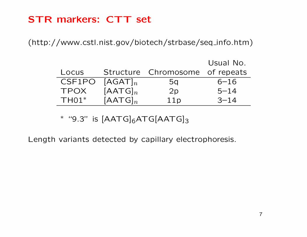
STR markers: CTT set
(http://www.cstl.nist.gov/biotech/strbase/seq info.htm)
Usual No.Locus Structure Chromosome of repeats
CSF1PO [AGAT]n 5q 6–16TPOX [AATG]n 2p 5–14TH01∗ [AATG]n 11p 3–14
∗ “9.3” is [AATG]6ATG[AATG]3
Length variants detected by capillary electrophoresis.
7

“CTT” Data - Forensic Frequency Database
CSF1P0 TPOX TH0111 12 8 11 7 811 13 8 8 6 711 12 8 11 6 710 12 8 8 6 911 12 8 12 9 9.310 12 9 11 6 710 13 8 11 6 611 12 8 8 6 9.39 10 8 9 7 9.311 12 8 8 6 811 13 8 11 7 911 12 8 11 6 9.310 11 8 8 7 9.310 10 8 11 7 9.39 10 8 8 6 9.311 12 9 11 9 9.39 11 9 11 9 9.311 12 8 8 6 710 10 9 11 6 9.310 13 8 8 8 9.3
8

Sequencing of STR Alleles
“STR typing in forensic genetics has been performed traditionally
using capillary electrophoresis (CE). Massively parallel sequenc-
ing (MPS) has been considered a viable technology in recent
years allowing high-throughput coverage at a relatively afford-
able price. Some of the CE-based limitations may be overcome
with the application of MPS ... generate reliable STR profiles
at a sensitivity level that competes with current widely used CE-
based method.”
Zeng XP, King JL, Stoljarova M, Warshauer DH, LaRue BL, Sa-
jantila A, Patel J, Storts DR, Budowle B. 2015. High sensitivity
multiplex short tandem repeat loci analyses with massively par-
allel sequencing. Forensic Science International: Genetics 16:38-
47.
9

Single Nucleotide Polymorphisms (SNPs)
“Single nucleotide polymorphisms (SNPs) are the most frequently
occurring genetic variation in the human genome, with the total
number of SNPs reported in public SNP databases currently ex-
ceeding 9 million. SNPs are important markers in many studies
that link sequence variations to phenotypic changes; such studies
are expected to advance the understanding of human physiology
and elucidate the molecular bases of diseases. For this reason,
over the past several years a great deal of effort has been devoted
to developing accurate, rapid, and cost-effective technologies for
SNP analysis, yielding a large number of distinct approaches. ”
Kim S. Misra A. 2007. SNP genotyping: technologies and
biomedical applications. Annu Rev Biomed Eng. 2007;9:289-
320.
10
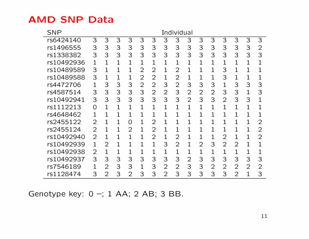
AMD SNP Data
SNP Individualrs6424140 3 3 3 3 3 3 3 3 3 3 3 3 3 3 3rs1496555 3 3 3 3 3 3 3 3 3 3 3 3 3 3 2rs1338382 3 3 3 3 3 3 3 3 3 3 3 3 3 3 3rs10492936 1 1 1 1 1 1 1 1 1 1 1 1 1 1 1rs10489589 3 1 1 1 2 2 1 2 1 1 1 3 1 1 1rs10489588 3 1 1 1 2 2 1 2 1 1 1 3 1 1 1rs4472706 1 3 3 3 2 2 3 2 3 3 3 1 3 3 3rs4587514 3 3 3 3 3 2 2 3 2 2 2 3 3 1 3rs10492941 3 3 3 3 3 3 3 3 2 3 3 2 3 3 1rs1112213 0 1 1 1 1 1 1 1 1 1 1 1 1 1 1rs4648462 1 1 1 1 1 1 1 1 1 1 1 1 1 1 1rs2455122 2 1 1 0 1 2 1 1 1 1 1 1 1 1 2rs2455124 2 1 1 2 1 2 1 1 1 1 1 1 1 1 2rs10492940 2 1 1 1 1 2 1 2 1 1 1 2 1 1 2rs10492939 1 2 1 1 1 1 3 2 1 2 3 2 2 1 1rs10492938 2 1 1 1 1 1 1 1 1 1 1 1 1 1 1rs10492937 3 3 3 3 3 3 3 3 2 3 3 3 3 3 3rs7546189 1 2 3 3 1 3 2 2 3 3 2 2 2 2 2rs1128474 3 2 3 2 3 3 2 3 3 3 3 3 2 1 3
Genotype key: 0 –; 1 AA; 2 AB; 3 BB.
11

Phase 3 1000Genomes Data
• 84.4 million variants
• 2504 individuals
• 26 populations
www.1000Genomes.org
12

Whole-genome Sequence Studies
One current study is the NHLBI Trans-Omics for Precision Medicine
(TOPMed) project. www.nhlbiwgs.org
In the first data freeze of Phase 1 of this study:
Abecasis et al. 2016. ASHG Poster. Currently 400 million SNVs
found from 73,000 whole-genome sequences.
13
Sampling
Statistical sampling: The variation among repeated samples
from the same population is analogous to “fixed” sampling. In-
ferences can be made about that particular population.
Genetic sampling: The variation among replicate (conceptual)
populations is analogous to “random” sampling. Inferences are
made to all populations with the same history.
14
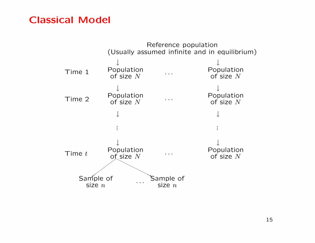
Classical Model
Sample ofsize n · · · Sample of
size n
��
��
���=
HHHHHHHHHHj
Time tPopulationof size N · · · Population
of size N
↓ ↓
... ...
↓ ↓
Time 2Populationof size N · · · Population
of size N
↓ ↓
Time 1 Populationof size N · · · Population
of size N
↓ ↓
Reference population(Usually assumed infinite and in equilibrium)
15

Coalescent Theory
An alternative framework works with genealogical history of a
sample of alleles. There is a tree linking all alleles in a current
sample to the “most recent common ancestral allele.” Allelic
variation due to mutations since that ancestral allele.
The coalescent approach requires mutation and may be more
appropriate for long-term evolution and analyses involving more
than one species. The classical approach allows mutation but
does not require it: within one species variation among popula-
tions may be due primarily to drift.
16

Probability
Probability provides the language of data analysis.
Equiprobable outcomes definition:
Probability of event E is number of outcomes favorable to E
divided by the total number of outcomes. e.g. Probability of a
head = 1/2.
Long-run frequency definition:
If event E occurs n times in N identical experiments, the prob-
ability of E is the limit of n/N as N goes to infinity.
Subjective probability:
Probability is a measure of belief.
17

First Law of Probability
Law says that probability can take values only in the range zero
to one and that an event which is certain has probability one.
0 ≤ Pr(E) ≤ 1
Pr(E|E) = 1 for any E
i.e. If event E is true, then it has a probability of 1. For example:
Pr(Seed is Round|Seed is Round) = 1
18

Second Law of Probability
If G and H are mutually exclusive events, then:
Pr(G or H) = Pr(G) + Pr(H)
For example,
Pr(Round or Wrinkled) = Pr(Round) + Pr(Wrinkled)
More generally, if Ei, i = 1, . . . r, are mutually exclusive then
Pr(E1 or . . . or Er) = Pr(E1) + . . .+ Pr(Er)
=∑
i
Pr(Ei)
19

Complementary Probability
If Pr(E) is the probability that E is true then Pr(E) denotes the
probability that E is false. Because these two events are mutually
exclusive
Pr(E or E) = Pr(E) + Pr(E)
and they are also exhaustive in that between them they cover all
possibilities – one or other of them must be true. So,
Pr(E) + Pr(E) = 1
Pr(E) = 1 − Pr(E)
The probability that E is false is one minus the probability it is
true.
20

Third Law of Probability
For any two events, G and H, the third law can be written:
Pr(G and H) = Pr(G) Pr(H|G)
There is no reason why G should precede H and the law can also
be written:
Pr(G and H) = Pr(H) Pr(G|H)
For example
Pr(Seed is round & is type AA)
= Pr(Seed is round|Seed is type AA) × Pr(Seed is type AA)
= 1 × p2A
21
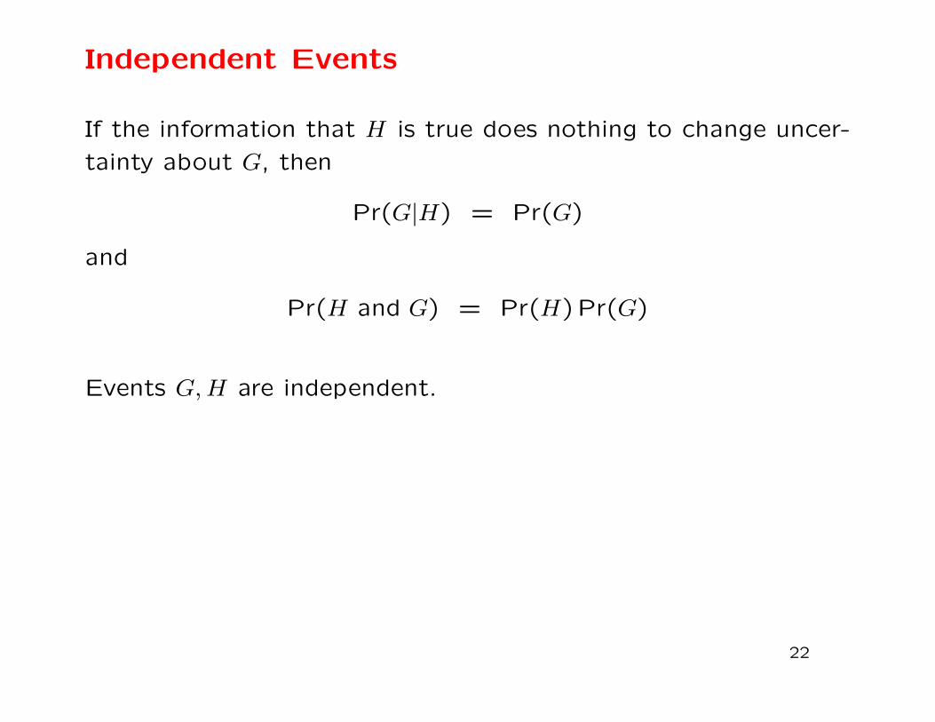
Independent Events
If the information that H is true does nothing to change uncer-
tainty about G, then
Pr(G|H) = Pr(G)
and
Pr(H and G) = Pr(H)Pr(G)
Events G,H are independent.
22
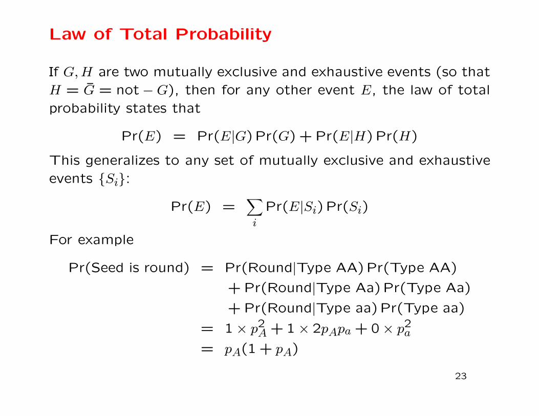
Law of Total Probability
If G,H are two mutually exclusive and exhaustive events (so that
H = G = not −G), then for any other event E, the law of total
probability states that
Pr(E) = Pr(E|G)Pr(G) + Pr(E|H) Pr(H)
This generalizes to any set of mutually exclusive and exhaustive
events {Si}:
Pr(E) =∑
i
Pr(E|Si)Pr(Si)
For example
Pr(Seed is round) = Pr(Round|Type AA)Pr(Type AA)
+ Pr(Round|Type Aa)Pr(Type Aa)
+ Pr(Round|Type aa)Pr(Type aa)
= 1 × p2A + 1 × 2pApa + 0 × p2a= pA(1 + pA)
23
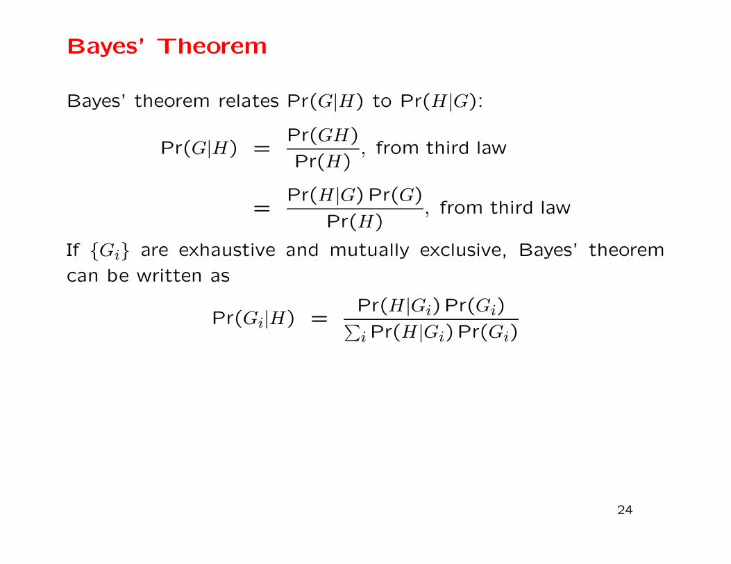
Bayes’ Theorem
Bayes’ theorem relates Pr(G|H) to Pr(H|G):
Pr(G|H) =Pr(GH)
Pr(H), from third law
=Pr(H|G) Pr(G)
Pr(H), from third law
If {Gi} are exhaustive and mutually exclusive, Bayes’ theorem
can be written as
Pr(Gi|H) =Pr(H|Gi)Pr(Gi)
∑
iPr(H|Gi)Pr(Gi)
24

Bayes’ Theorem Example
Suppose G is event that a man has genotype A1A2 and H is the
event that he transmits allele A1 to his child. Then Pr(H|G) =
0.5.
Now what is the probability that a man has genotype A1A2 given
that he transmits allele A1 to his child?
Pr(G|H) =Pr(H|G) Pr(G)
Pr(H)
=0.5 × 2p1p2
p1
= p2
25

Mendel’s Data
Model: seed shape governed by gene A with alleles A, a:
Genotype Phenotype
AA RoundAa Roundaa Wrinkled
Cross two inbred lines: AA and aa. All offspring (F1 generation)
are Aa, and so have round seeds.
26

F2 generation
Self an F1 plant: each allele it transmits is equally likely to be A
or a, and alleles are independent, so for F2 generation:
Pr(AA) = Pr(A)Pr(A) = 0.25
Pr(Aa) = Pr(A)Pr(a) + Pr(a)Pr(A) = 0.5
Pr(aa) = Pr(a)Pr(a) = 0.25
Probability that an F2 seed (observed on F1 parental plant) is
round:
Pr(Round) = Pr(Round|AA)Pr(AA)
+ Pr(Round|Aa)Pr(Aa)
+ Pr(Round|aa)Pr(aa)
= 1 × 0.25 + 1 × 0.5 + 0 × 0.25
= 0.75
27

F2 generation
What are the proportions of AA and Aa among F2 plants with
round seeds? From Bayes’ Theorem the predicted probability of
AA genotype, if the seed is round, is
Pr(F2 = AA|F2 Round) =Pr(F2 Round|AA)Pr(F2 AA)
Pr(F2 round)
=1 × 1
434
=1
3
28

Seed Characters
As an experimental check on this last result, and therefore on
Mendel’s theory, Mendel selfed a round-seeded F2 plant and
noted the F3 seed shape (observed on the F2 parental plant).
If all the F3 seeds are round, the F2 must have been AA. If some
F3 seed are round and some are wrinkled, the F2 must have been
Aa. Possible to observe many F3 seeds for an F2 parental plant,
so no doubt that all seeds were round. Data supported theory:
one-third of F2 plants gave only round seeds and so must have
had genotype AA.
29

Plant Characters
Model for stem length is
Genotype Phenotype
GG LongGg Longgg Short
To check this model it is necessary to grow the F3 seed to observe
the F3 stem length.
30
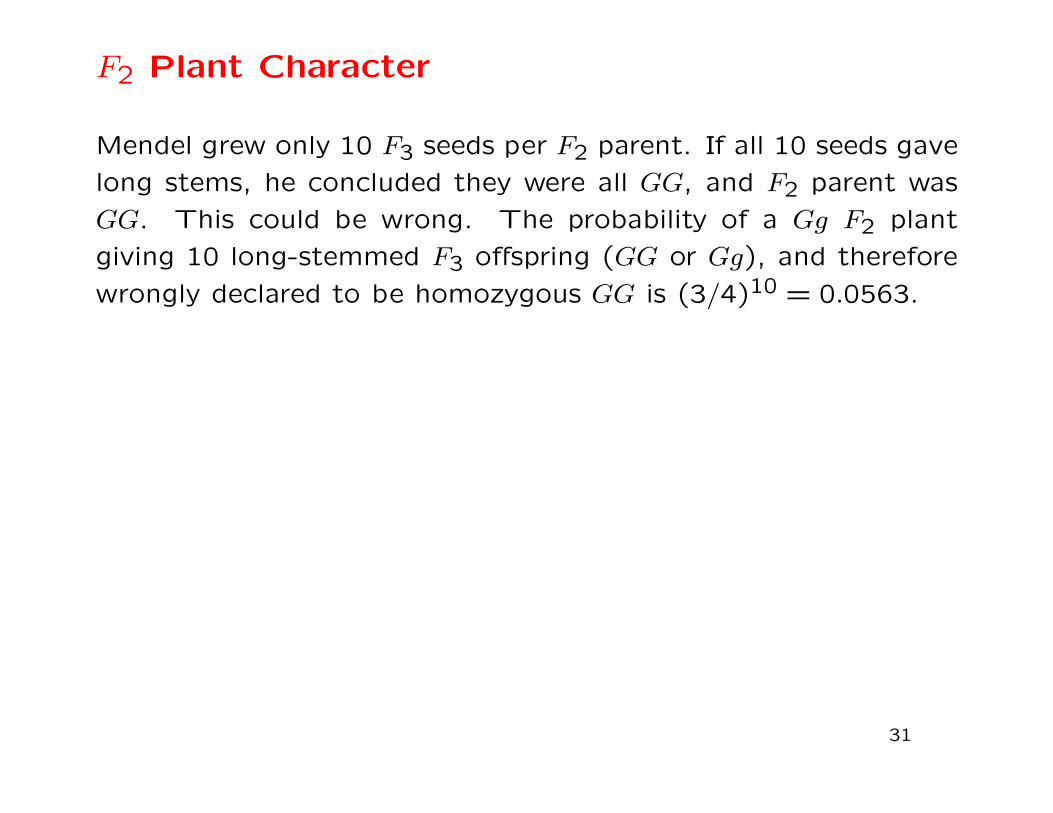
F2 Plant Character
Mendel grew only 10 F3 seeds per F2 parent. If all 10 seeds gave
long stems, he concluded they were all GG, and F2 parent was
GG. This could be wrong. The probability of a Gg F2 plant
giving 10 long-stemmed F3 offspring (GG or Gg), and therefore
wrongly declared to be homozygous GG is (3/4)10 = 0.0563.
31

Fisher’s 1936 Criticism
The probability that a long-stemmed F2 plant is declared to be
homozygous (event V ) is
Pr(V ) = Pr(V |U)Pr(U) + Pr(V |U)Pr(U)
= 1 × (1/3) + 0.0563 × (2/3)
= 0.3709
6= 1/3
where U is the event that a long-stemmed F2 is actually homozy-
gous and U is the event that it is actually heterozygous.
Fisher claimed Mendel’s data closer to the 0.3333 probability
appropriate for seed shape than to the correct 0.3709 value.
Mendel’s experiments were “a carefully planned demonstration
of his conclusions.”
32

Weldon’s 1902 Doubts
In Biometrika, Weldon said:
“Here are seven determinations of a frequency which is said toobey the law of Chance. Only one determination has a deviationfrom the hypothetical frequency greater than the probable errorof the determination, and one has a deviation sensible equal tothe probable error; so that a discrepancy between the hypothesisand the observations which is equal to or greater than the prob-able error occurs twice out of seven times, and deviations muchgreater than the probable error do not occur at all. These resultsthen accord so remarkably with Mendel’s summary of them thatif they were repeated a second time, under similar conditionsand on a similar scale, the chance that the agreement betweenobservation and hypothesis would be worse than that actuallyobtained is about 16 to 1.”
“Run Mendel’s experiments again at the same scale, Weldonreckoned, and the chance of getting worse results is 16 to 1.”Radick, Science 350:159-160, 2015.
33

Edwards’ 1986 Criticism
Mendel had 69 comparisons where the expected ratios were cor-
rect. Each set of data can be tested with a chi-square test:
Category 1 Category 2 Total
Observed (o) a n-a nExpected (e) b n-b n
X2 =(a− b)2
b+
[(n− a)− (n− b)]2
(n− b)
=n(a− b)2
b(n− b)
34

Edwards’ Criticism
If the hypothesis giving the expected values is true, the X2 val-
ues follow a chi-square distribution, and the X values follow a
normal distribution. Edwards claimed Mendel’s values were too
small – not as many large values as would be expected by chance.
−3.0−2.0−1.0 0.0 1.0 2.0 3.0
0.0
5.0
10.0
35

Recent Discussions
Franklin A, Edwards AWF, Fairbanks DJ, Hartl DL, Seidenfeld
T. “Ending the Mendel-Fisher Controversy.” University of Pitts-
burgh Press, Pittsburgh.
Smith MU, Gericke NM. 2015. Mendel in the modern classroom.
Science and Education 24:151-172.
Radick G. 2015. Beyond the “Mendel-Fisher controversy.” Sci-
ence 350:159-160.
Weeden NF. 2016. Are Mendel’s Data Reliable? The Per-
spective of a Pea Geneticist. Journal of Heredity 107:635-646.
“Mendel’s article is probably best regarded as his attempt to
present his model in a simple and convincing format with a min-
imum of additional details that might obscure his message.”
36

ALLELE FREQUENCIES
37

Properties of Estimators
Consistency Increasing accuracyas sample size increases
Unbiasedness Expected value is the parameter
Efficiency Smallest variance
Sufficiency Contains all the informationin the data about parameter
38

Binomial Distribution
Most population genetic data consists of numbers of observa-
tions in some categories. The values and frequencies of these
counts form a distribution.
Toss a coin n times, and note the number of heads. There
are (n+1) outcomes, and the number of times each outcome is
observed in many sets of n tosses gives the sampling distribution.
Or: sample n alleles from a population and observe x copies of
type A.
39
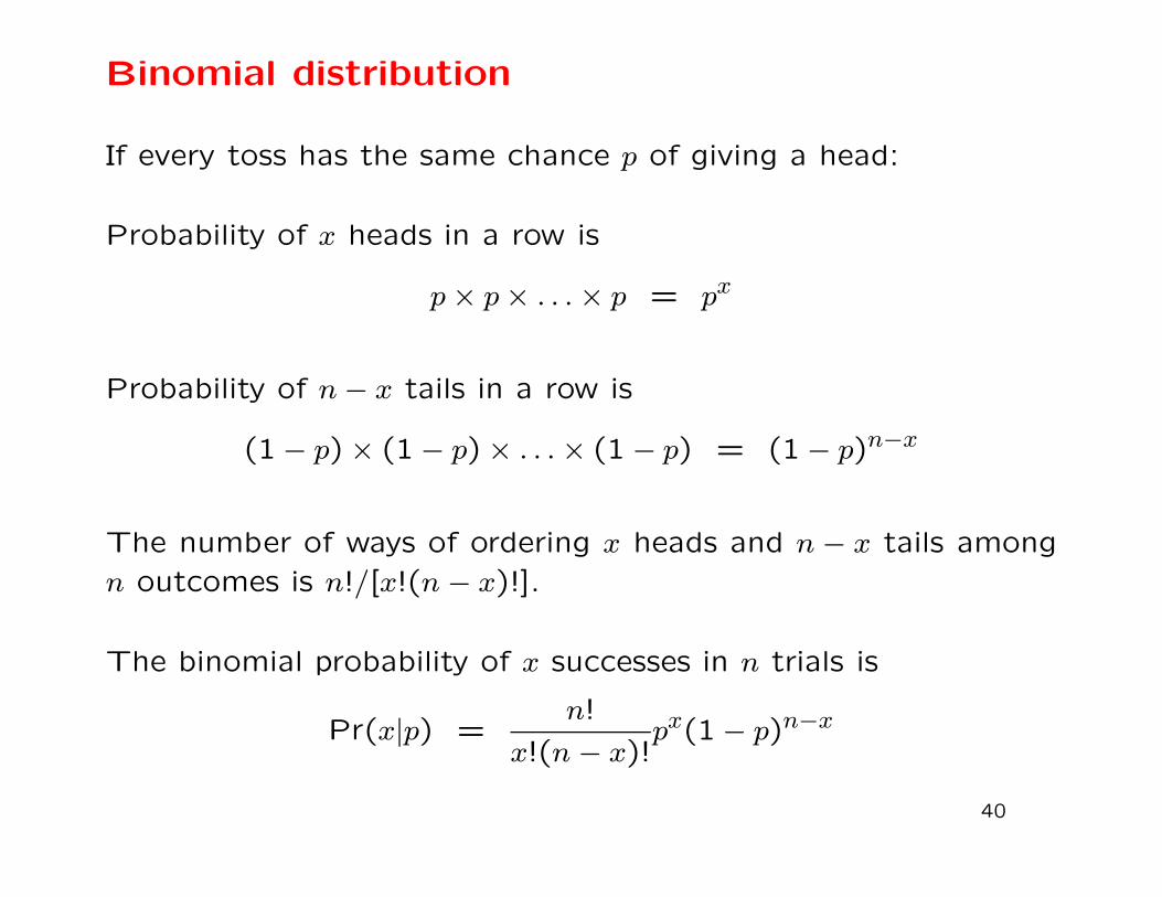
Binomial distribution
If every toss has the same chance p of giving a head:
Probability of x heads in a row is
p× p× . . .× p = px
Probability of n− x tails in a row is
(1 − p) × (1 − p) × . . .× (1 − p) = (1 − p)n−x
The number of ways of ordering x heads and n − x tails among
n outcomes is n!/[x!(n − x)!].
The binomial probability of x successes in n trials is
Pr(x|p) =n!
x!(n − x)!px(1 − p)n−x
40

Binomial Likelihood
The quantity Pr(x|p) is the probability of the data, x successes
in n trials, when each trial has probability p of success.
The same quantity, written as L(p|x), is the likelihood of the
parameter, p, when the value x has been observed. The terms
that do not involve p are not needed, so
L(p|x) ∝ px(1 − p)(n−x)
Each value of x gives a different likelihood curve, and each curve
points to a p value with maximum likelihood. This leads to
maximum likelihood estimation.
41

Likelihood L(p|x, n = 4)
42

Binomial Mean
If there are n trials, each of which has probability p of giving a
success, the mean or the expected number of successes is np.
The sample proportion of successes is
p =x
n
(This is also the maximum likelihood estimate of p.)
The expected, or mean, value of p is p.
E(p) = p
43

Binomial Variance
The expected value of the squared difference between the num-
ber of successes and its mean, (x − np)2, is np(1 − p). This is
the variance of the number of successes in n trials, and indicates
the spread of the distribution.
The variance of the sample proportion p is
Var(p) =p(1 − p)
n
44

Normal Approximation
Provided np is not too small (e.g. not less than 5), the binomial
distribution can be approximated by the normal distribution with
the same mean and variance. In particular:
p ∼ N
(
p,p(1 − p)
n
)
To use the normal distribution in practice, change to the standard
normal variable z with a mean of 0, and a variance of 1:
z =p− p
√
p(1 − p)/n
For a standard normal, 95% of the values lie between ±1.96.
The normal approximation to the binomial therefore implies that
95% of the values of p lie in the range
p ± 1.96√
p(1 − p)/n
45

Confidence Intervals
A 95% confidence interval is a variable quantity. It has end-
points which vary with the sample. Expect that 95% of samples
will lead to an interval that includes the unknown true value p.
The standard normal variable z has 95% of its values between
−1.96 and +1.96. This suggests that a 95% confidence interval
for the binomial parameter p is
p ± 1.96
√
p(1 − p)
n
46
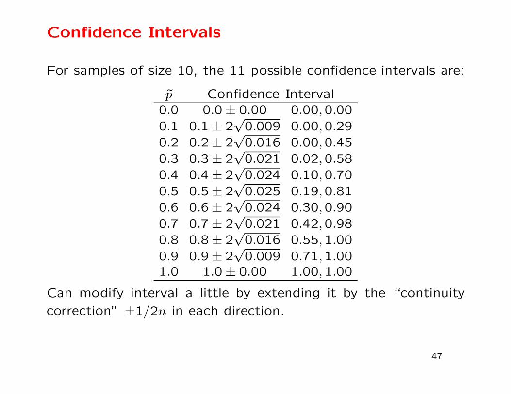
Confidence Intervals
For samples of size 10, the 11 possible confidence intervals are:
p Confidence Interval
0.0 0.0 ± 0.00 0.00,0.00
0.1 0.1 ± 2√
0.009 0.00,0.29
0.2 0.2 ± 2√
0.016 0.00,0.45
0.3 0.3 ± 2√
0.021 0.02,0.58
0.4 0.4 ± 2√
0.024 0.10,0.70
0.5 0.5 ± 2√
0.025 0.19,0.81
0.6 0.6 ± 2√
0.024 0.30,0.90
0.7 0.7 ± 2√
0.021 0.42,0.98
0.8 0.8 ± 2√
0.016 0.55,1.00
0.9 0.9 ± 2√
0.009 0.71,1.001.0 1.0 ± 0.00 1.00,1.00
Can modify interval a little by extending it by the “continuity
correction” ±1/2n in each direction.
47
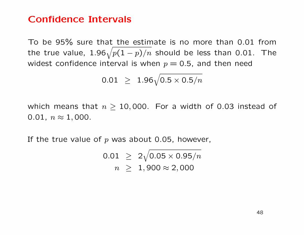
Confidence Intervals
To be 95% sure that the estimate is no more than 0.01 from
the true value, 1.96√
p(1 − p)/n should be less than 0.01. The
widest confidence interval is when p = 0.5, and then need
0.01 ≥ 1.96√
0.5 × 0.5/n
which means that n ≥ 10,000. For a width of 0.03 instead of
0.01, n ≈ 1,000.
If the true value of p was about 0.05, however,
0.01 ≥ 2√
0.05 × 0.95/n
n ≥ 1,900 ≈ 2,000
48

Exact Confidence Intervals: One-sided
The normal-based confidence intervals are constructed to be
symmetric about the sample value, unless the interval goes out-
side the interval from 0 to 1. They are therefore less satisfactory
the closer the true value is to 0 or 1.
More accurate confidence limits follow from the binomial distri-
bution exactly. For events with low probabilities p, how large
could p be for there to be at least a 5% chance of seeing no
more than x (i.e. 0,1,2, . . . x) occurrences of that event among
n events. If this upper bound is pU ,
x∑
k=0
Pr(k) ≥ 0.05
x∑
k=0
(
n
k
)
pkU(1 − pU)n−k ≥ 0.05
If x = 0, then (1 − pU)n ≥ 0.05 or pU ≤ 1 − 0.051/n and this is
0.0295 if n = 100. More generally pU ≈ 3/n when x = 0.
49
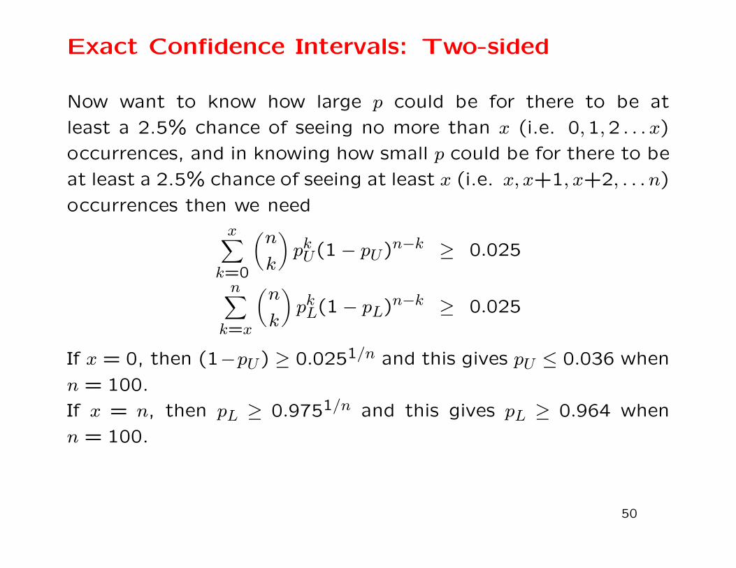
Exact Confidence Intervals: Two-sided
Now want to know how large p could be for there to be at
least a 2.5% chance of seeing no more than x (i.e. 0,1,2 . . . x)
occurrences, and in knowing how small p could be for there to be
at least a 2.5% chance of seeing at least x (i.e. x, x+1, x+2, . . . n)
occurrences then we need
x∑
k=0
(
n
k
)
pkU(1 − pU)n−k ≥ 0.025
n∑
k=x
(
n
k
)
pkL(1 − pL)n−k ≥ 0.025
If x = 0, then (1−pU) ≥ 0.0251/n and this gives pU ≤ 0.036 when
n = 100.
If x = n, then pL ≥ 0.9751/n and this gives pL ≥ 0.964 when
n = 100.
50

Bootstrapping
An alternative method for constructing confidence intervals uses
numerical resampling. A set of samples is drawn, with replace-
ment, from the original sample to mimic the variation among
samples from the original population. Each new sample is the
same size as the original sample, and is called a bootstrap sam-
ple.
The middle 95% of the sample values p from a large number of
bootstrap samples provides a 95% confidence interval.
51
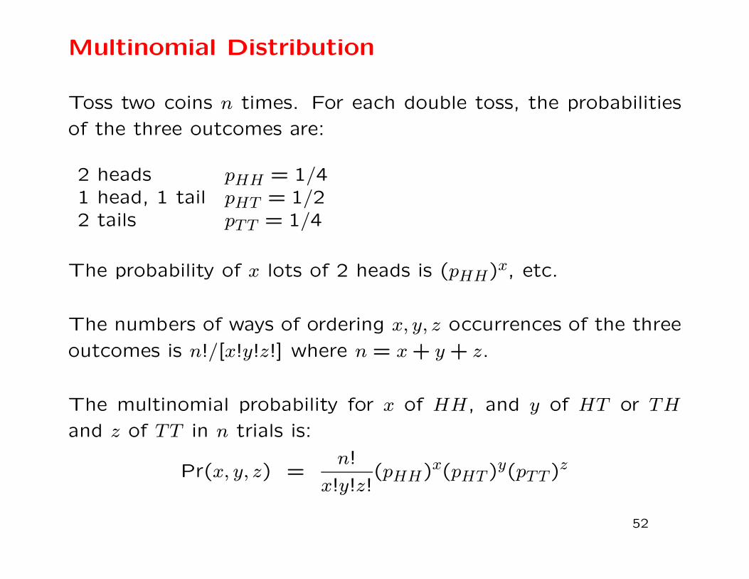
Multinomial Distribution
Toss two coins n times. For each double toss, the probabilities
of the three outcomes are:
2 heads pHH = 1/41 head, 1 tail pHT = 1/22 tails pTT = 1/4
The probability of x lots of 2 heads is (pHH)x, etc.
The numbers of ways of ordering x, y, z occurrences of the three
outcomes is n!/[x!y!z!] where n = x+ y+ z.
The multinomial probability for x of HH, and y of HT or TH
and z of TT in n trials is:
Pr(x, y, z) =n!
x!y!z!(pHH)x(pHT )y(pTT )z
52

Multinomial Variances and Covariances
If {pi} are the probabilities for a series of categories, the sam-
ple proportions pi from a sample of n observations have these
properties:
E(pi) = pi
Var(pi) =1
npi(1 − pi)
Cov(pi, pj) = −1
npipj, i 6= j
The covariance is defined as E[(pi − pi)(pj − pj)].
For the sample counts:
E(ni) = npi
Var(ni) = npi(1 − pi)
Cov(ni, nj) = −npipj, i 6= j
53
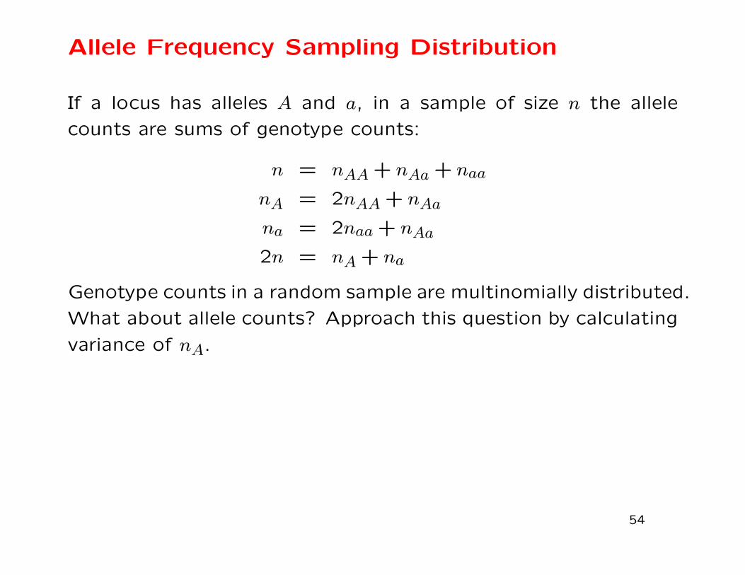
Allele Frequency Sampling Distribution
If a locus has alleles A and a, in a sample of size n the allele
counts are sums of genotype counts:
n = nAA + nAa + naa
nA = 2nAA + nAa
na = 2naa + nAa
2n = nA + na
Genotype counts in a random sample are multinomially distributed.
What about allele counts? Approach this question by calculating
variance of nA.
54
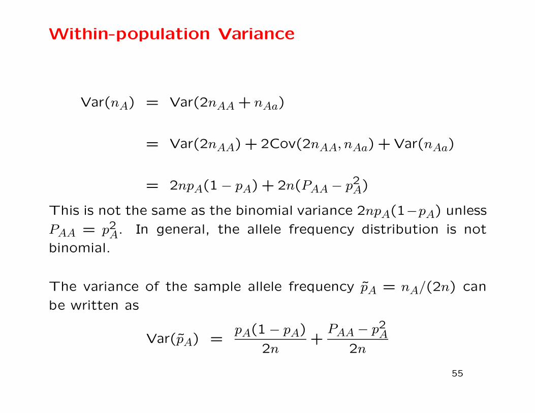
Within-population Variance
Var(nA) = Var(2nAA + nAa)
= Var(2nAA) + 2Cov(2nAA, nAa) + Var(nAa)
= 2npA(1 − pA) + 2n(PAA− p2A)
This is not the same as the binomial variance 2npA(1−pA) unless
PAA = p2A. In general, the allele frequency distribution is not
binomial.
The variance of the sample allele frequency pA = nA/(2n) can
be written as
Var(pA) =pA(1 − pA)
2n+PAA− p2A
2n
55
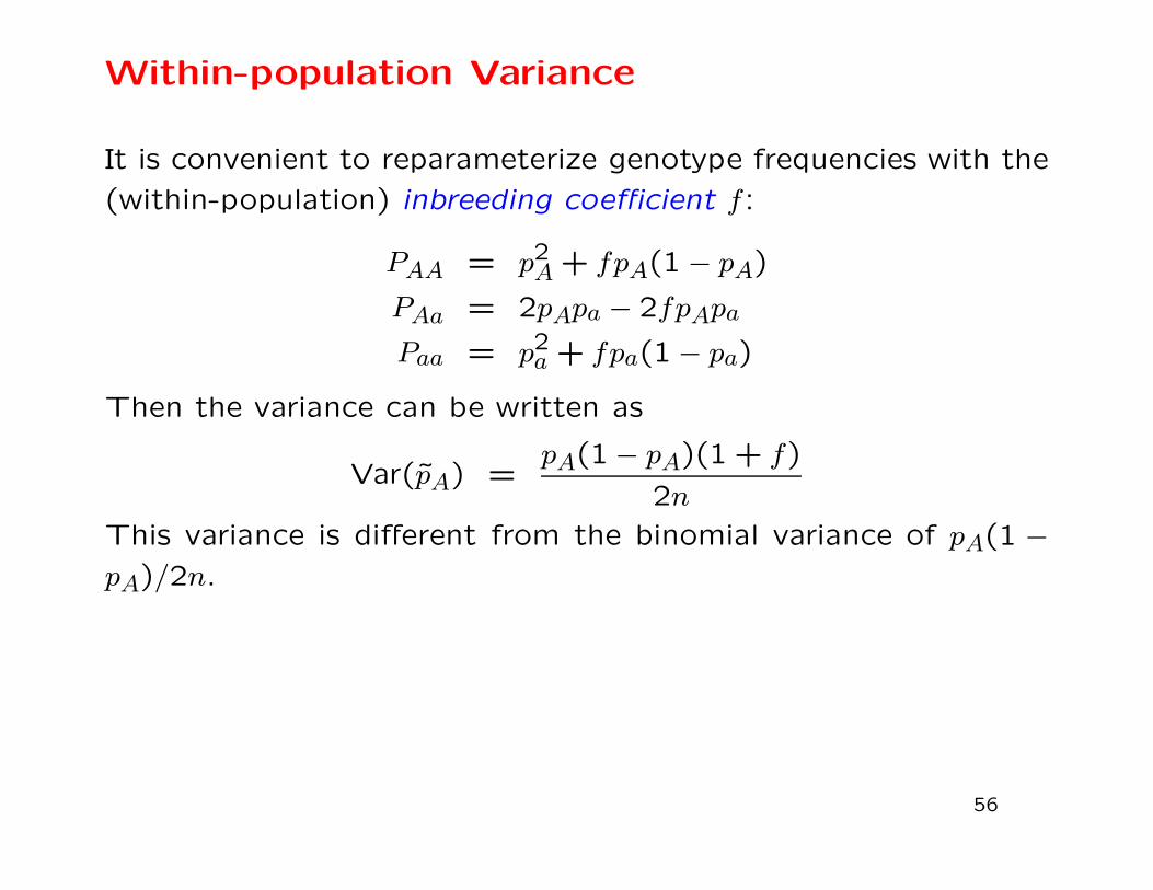
Within-population Variance
It is convenient to reparameterize genotype frequencies with the
(within-population) inbreeding coefficient f :
PAA = p2A + fpA(1 − pA)
PAa = 2pApa − 2fpApa
Paa = p2a + fpa(1 − pa)
Then the variance can be written as
Var(pA) =pA(1 − pA)(1 + f)
2n
This variance is different from the binomial variance of pA(1 −pA)/2n.
56

Bounds on f
Since
pA ≥ PAA = p2A + fpA(1 − pA) ≥ 0
pa ≥ Paa = p2a + fpa(1 − pa) ≥ 0
there are bounds on f :
−pA/(1 − pA) ≤ f ≤ 1
−pa/(1 − pa) ≤ f ≤ 1
or
max
(
−pApa,−papA
)
≤ f ≤ 1
This range of values is [-1,1] when pA = pa.
57
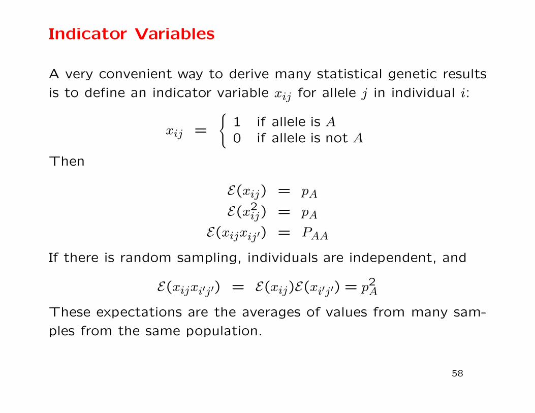
Indicator Variables
A very convenient way to derive many statistical genetic results
is to define an indicator variable xij for allele j in individual i:
xij =
{
1 if allele is A0 if allele is not A
Then
E(xij) = pA
E(x2ij) = pA
E(xijxij′) = PAA
If there is random sampling, individuals are independent, and
E(xijxi′j′) = E(xij)E(xi′j′) = p2A
These expectations are the averages of values from many sam-
ples from the same population.
58
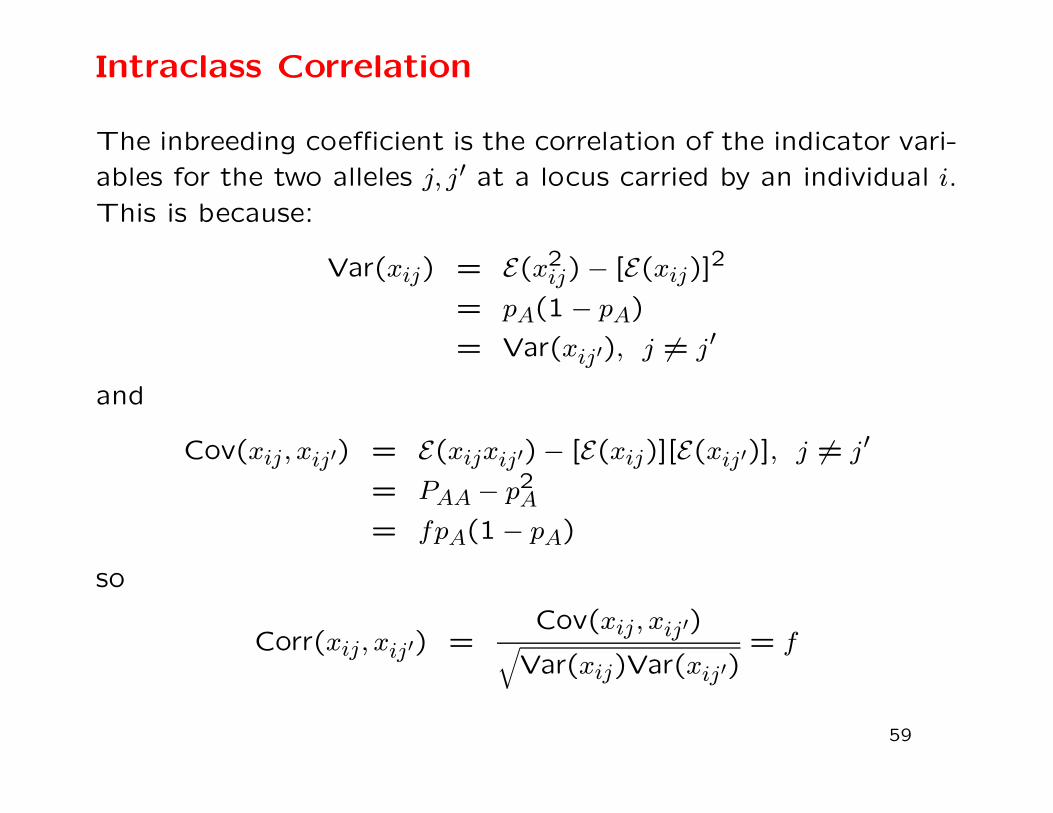
Intraclass Correlation
The inbreeding coefficient is the correlation of the indicator vari-
ables for the two alleles j, j′ at a locus carried by an individual i.
This is because:
Var(xij) = E(x2ij) − [E(xij)]2
= pA(1 − pA)
= Var(xij′), j 6= j′
and
Cov(xij , xij′) = E(xijxij′)− [E(xij)][E(xij′)], j 6= j′
= PAA− p2A= fpA(1 − pA)
so
Corr(xij, xij′) =Cov(xij , xij′)
√
Var(xij)Var(xij′)= f
59

Maximum Likelihood Estimation: Binomial
For binomial sample of size n, the likelihood of pA for nA alleles
of type A is
L(pA|nA) = C(pA)nA(1 − pA)n−nA
and is maximized when
∂L(pA|nA)
∂pA= 0 or when
∂ lnL(pA|na)∂pA
= 0
Now
lnL(pA|nA) = lnC + nA ln(pA) + (n− nA) ln(1 − pA)
so
∂ lnL(pA|nA)
∂pA=
nApA
− n− nA1 − pA
and this is zero when pA = pA = nA/n.
60
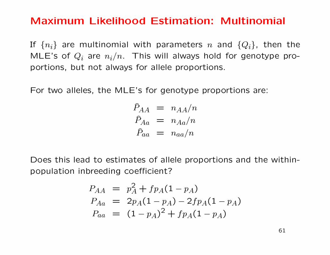
Maximum Likelihood Estimation: Multinomial
If {ni} are multinomial with parameters n and {Qi}, then the
MLE’s of Qi are ni/n. This will always hold for genotype pro-
portions, but not always for allele proportions.
For two alleles, the MLE’s for genotype proportions are:
PAA = nAA/n
PAa = nAa/n
Paa = naa/n
Does this lead to estimates of allele proportions and the within-
population inbreeding coefficient?
PAA = p2A + fpA(1 − pA)
PAa = 2pA(1 − pA)− 2fpA(1 − pA)
Paa = (1 − pA)2 + fpA(1 − pA)
61

Maximum Likelihood Estimation
The likelihood function for pA, f is
L(pA, f) =n!
nAA!nAa!naa![p2A + pA(1 − pA)f ]nAA
×[2pA(1 − pA)f ]nAa[(1 − pA)2 + pA(1 − pA)f ]naa
and it is difficult to find, analytically, the values of pA and f that
maximize this function or its logarithm.
There is an alternative way of finding maximum likelihood esti-
mates in this case: equating the observed and expected values
of the genotype frequencies.
62
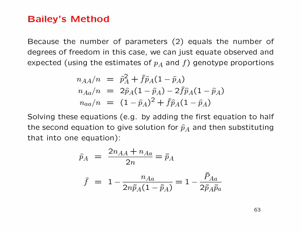
Bailey’s Method
Because the number of parameters (2) equals the number of
degrees of freedom in this case, we can just equate observed and
expected (using the estimates of pA and f) genotype proportions
nAA/n = p2A + f pA(1 − pA)
nAa/n = 2pA(1 − pA) − 2f pA(1 − pA)
naa/n = (1 − pA)2 + f pA(1 − pA)
Solving these equations (e.g. by adding the first equation to half
the second equation to give solution for pA and then substituting
that into one equation):
pA =2nAA + nAa
2n= pA
f = 1 − nAa2npA(1 − pA)
= 1 − PAa2pApa
63

Three-allele Case
With three alleles, there are six genotypes and 5 df. To use
Bailey’s method, would need five parameters: 2 allele frequencies
and 3 inbreeding coefficients:
P11 = p21 + f12p1p2 + f13p1p3
P12 = 2p1p2 − 2f12p1p2
P22 = p22 + f12p1p2 + f23p2p3
P13 = 2p1p3 − 2f13p1p3
P23 = 2p2p3 − 2f23p2p3
P33 = p23 + f13p1p3 + f23p2p3
We would generally prefer to have only one inbreeding coefficient
f . It is a difficult numerical problem to find the MLE for f .
64
Method of Moments
An alternative to maximum likelihood estimation is the method
of moments (MoM) where observed values of statistics are set
equal to their expected values. In general, this does not lead to
unique estimates or to estimates with variances as small as those
for maximum likelihood. (Bailey’s method is for the special case
where the MLEs are also MoM estimates.)
65
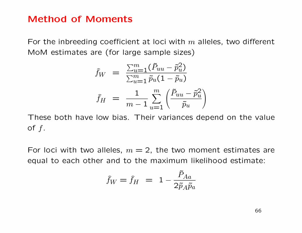
Method of Moments
For the inbreeding coefficient at loci with m alleles, two different
MoM estimates are (for large sample sizes)
fW =
∑mu=1(Puu − p2u)
∑mu=1 pu(1 − pu)
fH =1
m− 1
m∑
u=1
(
Puu − p2upu
)
These both have low bias. Their variances depend on the value
of f .
For loci with two alleles, m = 2, the two moment estimates are
equal to each other and to the maximum likelihood estimate:
fW = fH = 1 − PAa2pApa
66

MLE for Recessive Alleles
Suppose allele a is recessive to allele A. If there is Hardy-
Weinberg equilibrium, the likelihood for the two phenotypes is
L(pa) = (1 − p2a)n−naa(p2a)
naa
ln(L(pa) = (n− naa) ln(1 − p2a) + 2naa ln(pa)
where there are naa individuals of type aa and n− naa of type A.
Differentiating wrt pa:
∂ lnL(pa)
∂pa= −2pa(n− naa)
1 − p2a+
2naa
pa
Setting this to zero leads to an equation that can be solved
explicitly: p2a = naa/n. No need for iteration.
67

EM Algorithm for Recessive Alleles
An alternative way of finding maximum likelihood estimates when
there are “missing data” involves Estimation of the missing data
and then Maximization of the likelihood. For a locus with allele A
dominant to a the missing information is the frequencies (1−pa)2of AA, and 2pa(1−pa) of Aa genotypes. Only the joint frequency
(1 − p2a) of AA+Aa can be observed.
Estimate the missing genotype counts (assuming independence
of alleles) as proportions of the total count of dominant pheno-
types:
nAA =(1 − pa)2
1 − p2a(n− naa) =
(1 − pa)(n − naa)
(1 + pa)
nAa =2pa(1 − pa)
1 − p2a(n− naa) =
2pa(n− naa)
(1 + pa)
68

EM Algorithm for Recessive Alleles
Maximize the likelihood (using Bailey’s method):
pa =nAa + 2naa
2n
=1
2n
(
2pa(n− naa)
(1 + pa)+ 2naa
)
=2(npa + naa)
2n(1 + pa)
An initial estimate pa is put into the right hand side to give an
updated estimated pa on the left hand side. This is then put
back into the right hand side to give an iterative equation for pa.
This procedure also has explicit solution pa =√
(naa/n).
69
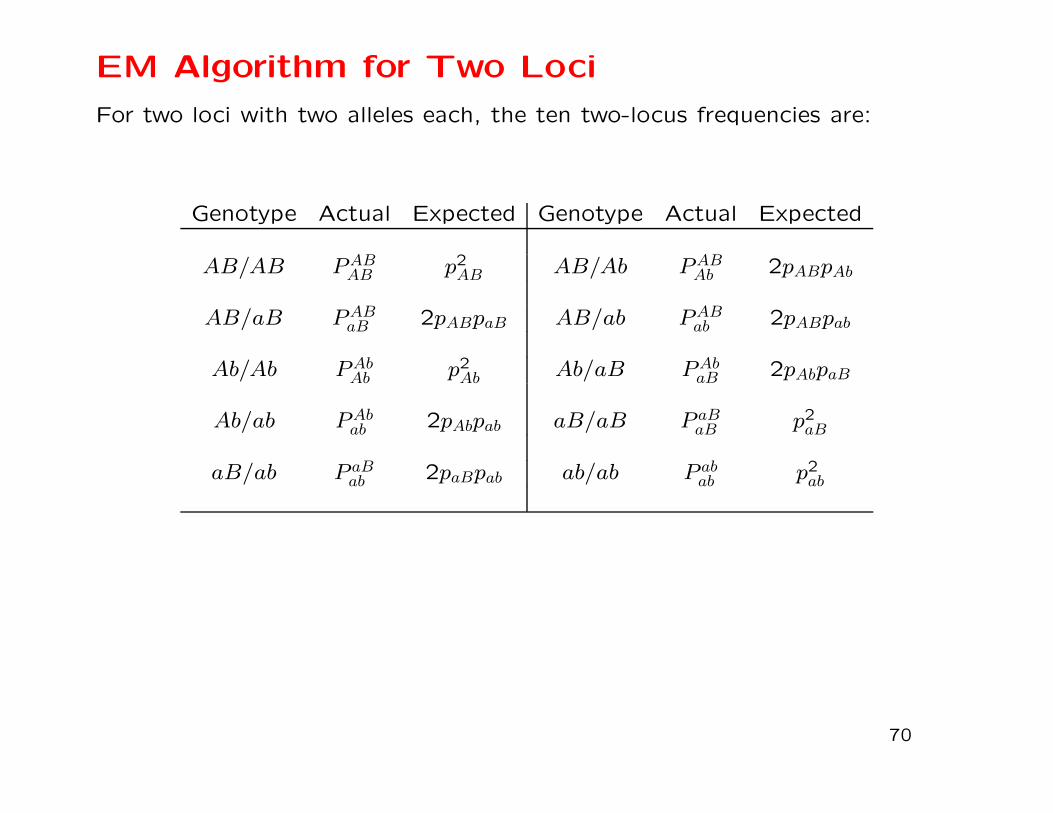
EM Algorithm for Two Loci
For two loci with two alleles each, the ten two-locus frequencies are:
Genotype Actual Expected Genotype Actual Expected
AB/AB PABAB p2AB AB/Ab PAB
Ab 2pABpAb
AB/aB PABaB 2pABpaB AB/ab PAB
ab 2pABpab
Ab/Ab PAbAb p2Ab Ab/aB PAb
aB 2pAbpaB
Ab/ab PAbab 2pAbpab aB/aB P aB
aB p2aB
aB/ab P aBab 2paBpab ab/ab P ab
ab p2ab
70

EM Algorithm for Two Loci
Gamete frequencies are marginal sums:
pAB = PABAB +1
2(PABAb + PABaB + PABab )
pAb = PAbAb +1
2(PAbAB + PAbab + PAbaB)
paB = P aBaB +1
2(P aBAB + P aBab + P aBAb )
pab = P abab +1
2(P abAb + P abaB + P abAB)
Can arrange gamete frequencies as two-way table to show that
only one of them is unknown when the allele frequencies are
known:
pAB pAb pApaB pab papB pb 1
71

EM Algorithm for Two Loci
The two double heterozygote frequencies PABab , PAbaB are “missing
data.”
Assume initial value of pAB and Estimate the missing counts as
proportions of the total count of double heterozygotes:
nABab =2pABpab
2pABpab + 2pAbpaBnAaBb
nAbaB =2pAbpaB
2pABpab + 2pAbpaBnAaBb
and then Maximize the likelihood by setting
pAB =1
2n
(
2nABAB + nABAb + nABaB + nABab
)
72

Example
As an example, consider the data
BB Bb bb Total
AA nAABB = 5 nAABb = 3 nAAbb = 2 nAA = 10Aa nAaBB = 3 nAaBb = 2 nAabb = 0 nAa = 5aa naaBB = 0 naaBb = 0 naabb = 0 naa = 0
Total nBB = 8 nBb = 5 nbb = 2 n = 15
There is one unknown gamete count x = nAB for AB:
B b Total
A nAB = x nAb = 25 − x nA = 25a naB = 21 − x nab = x− 16 na = 5
Total nB = 21 nb = 9 2n = 30
21 ≥ x ≥ 16
73

Example
EM iterative equation:
x′ = 2nAABB + nAABb + nAaBB + nAB/ab
= 2nAABB + nAABb + nAaBB +2pABpab
2pABpab + 2pAbpaBnAaBb
= 10 + 3 + 3 + 2 × 2x(x − 16)
2x(x− 16) + 2(25 − x)(21 − x)
= 16 +x(x− 16)
x(x− 16) + (25 − x)(21 − x)
In this case note that if x = 16 then x′ = 16 so this is the MLE.
74

Example
If we did not recognize the solution, a good starting value would
assume independence of A and B alleles: x = 2n ∗ pA ∗ pB =
(25 × 21/30) = 17.5.
Successive iterates are:
Iterate x value
0 17.50001 17.00002 16.69393 16.48934 16.34735 16.2472... ...
The solution is actually x = 16. This particular example does
not have convergence to the MLE for some starting values for
x.
75

ALLELIC ASSOCIATION
76

Hardy-Weinberg Law
For a random mating population, expect that genotype frequen-
cies are products of allele frequencies.
For a locus with two alleles, A, a:
PAA = (pA)2
PAa = 2pApa
Paa = (pa)2
These are also the results of setting the inbreeding coefficient f
to zero.
For a locus with several alleles Ai:
PAiAi = (pAi)2
PAiAj = 2pAipAj
77
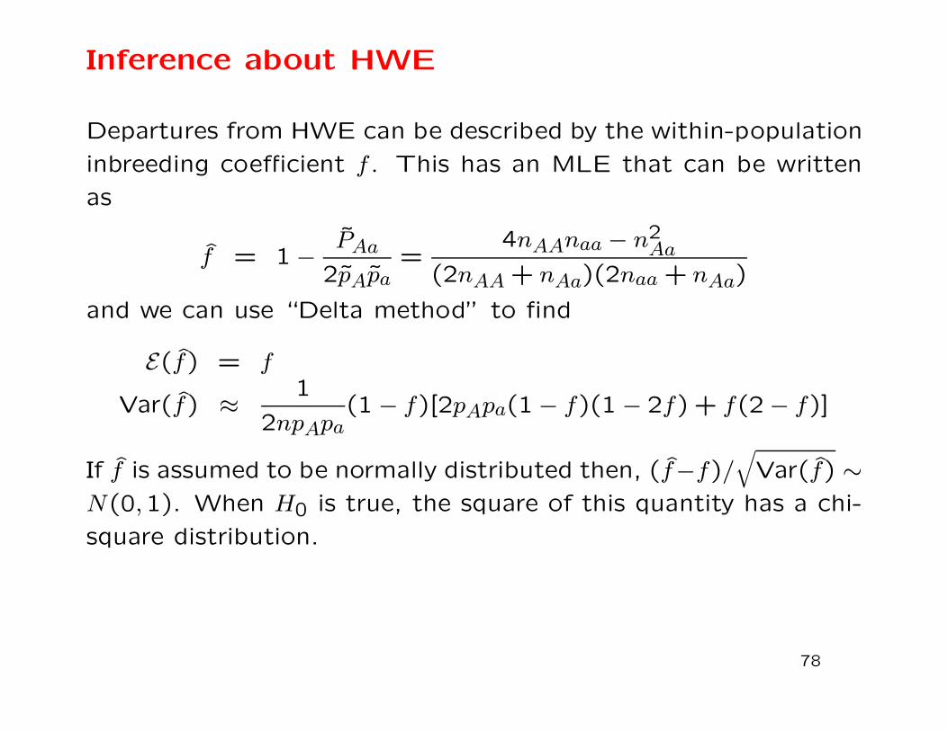
Inference about HWE
Departures from HWE can be described by the within-population
inbreeding coefficient f . This has an MLE that can be written
as
f = 1 − PAa2pApa
=4nAAnaa − n2
Aa
(2nAA + nAa)(2naa + nAa)
and we can use “Delta method” to find
E(f) = f
Var(f) ≈ 1
2npApa(1 − f)[2pApa(1 − f)(1 − 2f) + f(2 − f)]
If f is assumed to be normally distributed then, (f−f)/√
Var(f) ∼N(0,1). When H0 is true, the square of this quantity has a chi-
square distribution.
78

Inference about HWE
Since Var(f) = 1/n when f = 0:
X2 =
f − f√
Var(f)
2
=f2
1/n
= nf2
is appropriate for testing H0 : f = 0. When H0 is true, X2 ∼ χ2(1)
.
Reject HWE if X2 > 3.84.
79

Significance level of HWE test
0 1 2 3 4 5
0.0
0.2
0.4
0.6
0.8
1.0
Chi−square with 1 df
X^2
f(X
^2)
Probability=0.05
X^2=3.84
The area under the chi-square curve to the right of X2 = 3.84
is the probability of rejecting HWE when HWE is true. This is
the significance level of the test.
80

Goodness-of-fit Test
An alternative, but equivalent, test is the goodness-of-fit test.
Genotype Observed Expected (Obs.−Exp.)2
Exp.
AA nAA np2A np2af2
Aa nAa 2npApa 2npApaf2
aa naa np2a np2Af2
The test statistic is
X2 =∑ (Obs.− Exp)2
Exp.= nf2
81

Goodness-of-fit Test
Does a sample of 6 AA, 3 Aa, 1 aa support Hardy-Weinberg?
First need to estimate allele frequencies:
pA = PAA +1
2PAa = 0.75
pa = Paa +1
2PAa = 0.25
Then form “expected” counts:
nAA = n(pA)2 = 5.625
nAa = 2npApa = 3.750
naa = n(pa)2 = 0.625
82
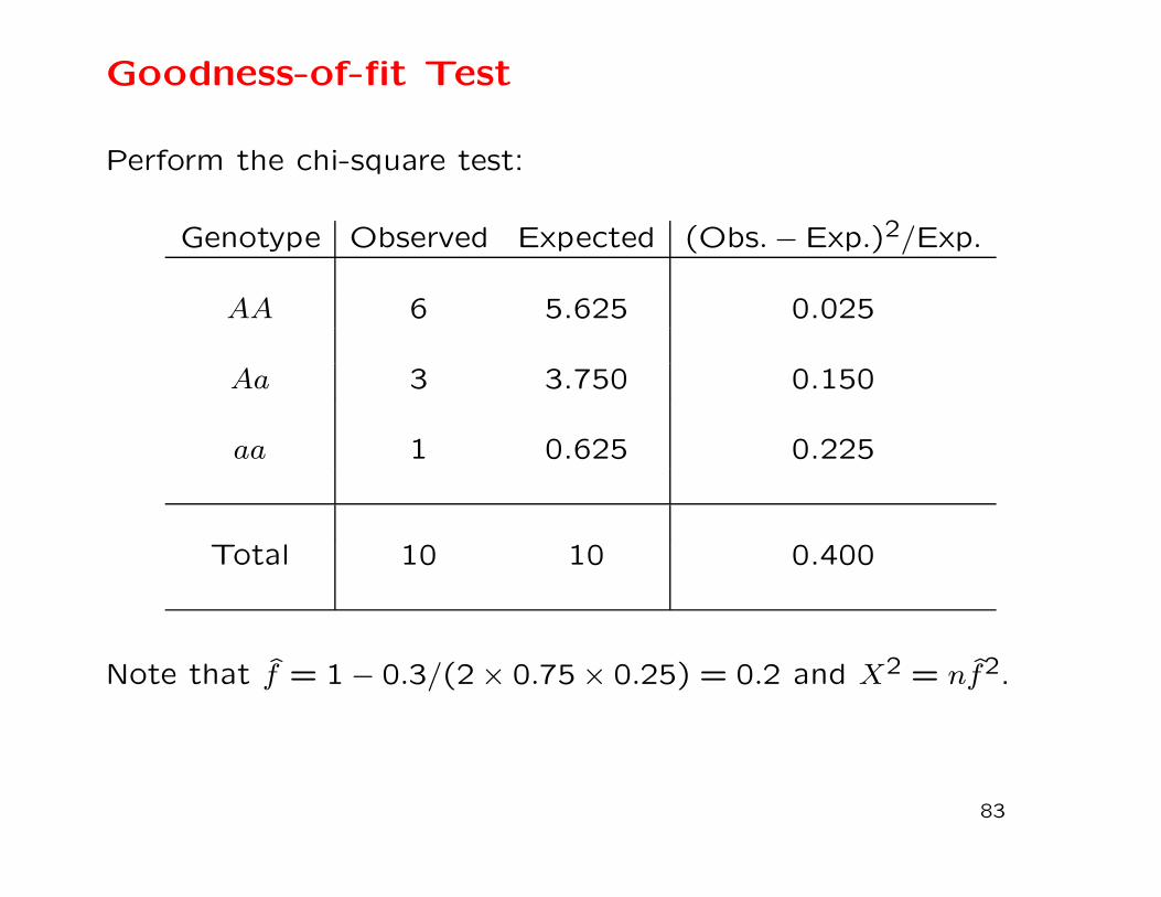
Goodness-of-fit Test
Perform the chi-square test:
Genotype Observed Expected (Obs.− Exp.)2/Exp.
AA 6 5.625 0.025
Aa 3 3.750 0.150
aa 1 0.625 0.225
Total 10 10 0.400
Note that f = 1 − 0.3/(2 × 0.75 × 0.25) = 0.2 and X2 = nf2.
83
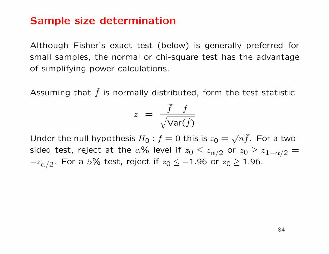
Sample size determination
Although Fisher’s exact test (below) is generally preferred for
small samples, the normal or chi-square test has the advantage
of simplifying power calculations.
Assuming that f is normally distributed, form the test statistic
z =f − f
√
Var(f)
Under the null hypothesis H0 : f = 0 this is z0 =√nf . For a two-
sided test, reject at the α% level if z0 ≤ zα/2 or z0 ≥ z1−α/2 =
−zα/2. For a 5% test, reject if z0 ≤ −1.96 or z0 ≥ 1.96.
84
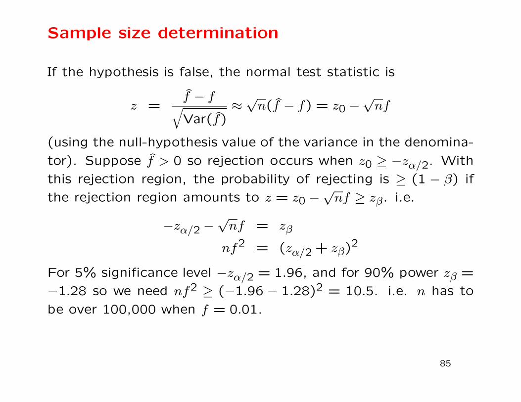
Sample size determination
If the hypothesis is false, the normal test statistic is
z =f − f
√
Var(f)≈
√n(f − f) = z0 −
√nf
(using the null-hypothesis value of the variance in the denomina-
tor). Suppose f > 0 so rejection occurs when z0 ≥ −zα/2. With
this rejection region, the probability of rejecting is ≥ (1 − β) if
the rejection region amounts to z = z0 −√nf ≥ zβ. i.e.
−zα/2 −√nf = zβ
nf2 = (zα/2 + zβ)2
For 5% significance level −zα/2 = 1.96, and for 90% power zβ =
−1.28 so we need nf2 ≥ (−1.96 − 1.28)2 = 10.5. i.e. n has to
be over 100,000 when f = 0.01.
85
Sample size determination
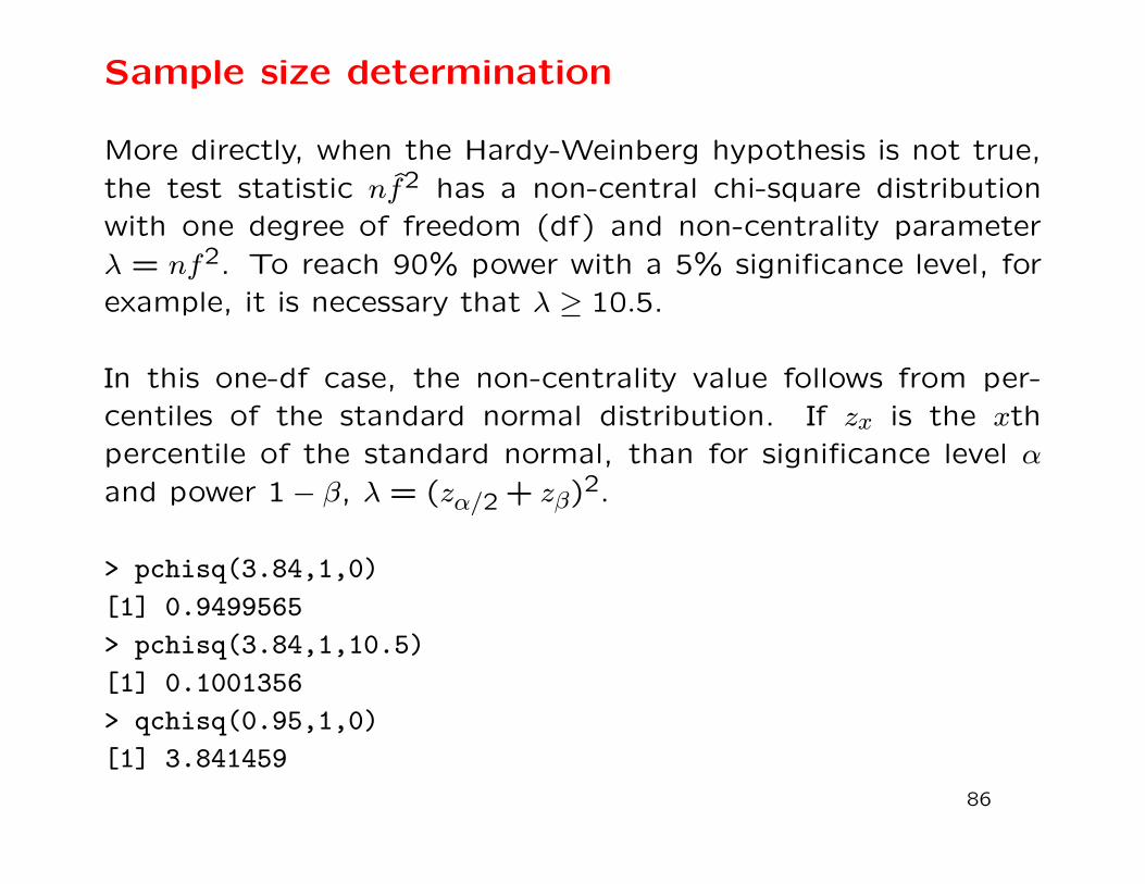
More directly, when the Hardy-Weinberg hypothesis is not true,
the test statistic nf2 has a non-central chi-square distribution
with one degree of freedom (df) and non-centrality parameter
λ = nf2. To reach 90% power with a 5% significance level, for
example, it is necessary that λ ≥ 10.5.
In this one-df case, the non-centrality value follows from per-
centiles of the standard normal distribution. If zx is the xth
percentile of the standard normal, than for significance level α
and power 1 − β, λ = (zα/2 + zβ)2.
> pchisq(3.84,1,0)
[1] 0.9499565
> pchisq(3.84,1,10.5)
[1] 0.1001356
> qchisq(0.95,1,0)
[1] 3.841459
86

Power of HWE test
0 5 10 15 20 25 30
0.0
00.0
20.0
40.0
60.0
8
Non−central Chi−square with 1 df, ncp=10.5
X^2
f(X
^2)
Probability=0.90
X^2=3.84
The area under the non-central chi-square curve to the right
of X2 = 3.84 is the probability of rejecting HWE when HWE
is false. This is the power of the test. In this plot, the non-
centrality parameter is λ = 10.5.
87

Population Structure: Departures from HWE
If a population consists of a number of subpopulations, each in
HWE but with different allele frequencies, there will be a depar-
ture from HWE at the population level. This is the Wahlund
effect.
Suppose there are two equal-sized subpopulations, each in HWE
but with different allele frequencies, then
Subpopn 1 Subpopn 2 Total Popn
pA 0.6 0.4 0.5pa 0.4 0.6 0.5
PAA 0.36 0.16 0.26 > (0.5)2
PAa 0.48 0.48 0.48 < 2(0.5)(0.5)
Paa 0.16 0.36 0.26 > (0.5)2
88

Population Admixture: Departures from HWE
A population might represent the recent admixture of two parentalpopulations. With the same two populations as before but now
with 1/4 of marriages within population 1, 1/2 of marriages
between populations 1 and 2, and 1/4 of marriages within pop-
ulation 2. If children with one or two parents in population 1 are
considered as belonging to population 1, there is an excess of
heterozygosity in the offspring population.
If the proportions of marriages within populations 1 and 2 are
both 25% and the proportion between populations 1 and 2 is
50%, the next generation has
Population 1 Population 2
PAA 0.09 + 0.12 = 0.21 0.04PAa 0.12 + 0.26 = 0.38 0.12Paa 0.04 + 0.12 = 0.16 0.09
0.75 0.25
Population 2 is in HWE, but Population 2 has 51% heterozygotes
instead of the expected 49.8%.
89

Significance Levels and p-values
The significance level α of a test is the probability of a false
rejection. It is specified by the user, and along with the null
hypothesis, it determines the rejection region. The specified, or
“nominal” value may not be achieved for an actual test.
Once the test has been conducted on a data set, the probability
of the observed test statistic, or a more extreme value, if the
null hypothesis is true is the p-value. The chi-square and normal
tests shown above give approximate p-values because they use a
continuous distribution for discrete data.
An alternative class of tests, “exact tests,” use a discrete distri-
bution for discrete data and provide accurate p-values. It may
be difficult to construct an exact test with a particular nominal
significance level.
90

Exact HWE Test
The preferred test for HWE is an exact one. The test rests
on the assumption that individuals are sampled randomly from
a population so that genotype counts have a multinomial distri-
bution:
Pr(nAA, nAa, naa) =n!
nAA!nAa!naa!(PAA)nAA(PAa)
nAa(Paa)naa
This equation is always true, and when there is HWE (PAA = p2Aetc.) there is the additional result that the allele counts have a
binomial distribution:
Pr(nA, na) =(2n)!
nA!na!(pA)nA(pa)
na
91

Exact HWE Test
Putting these together gives the conditional probability
Pr(nAA, nAa, naa|nA, na) =Pr(nAA, nAa, naa and nA, na)
Pr(nA, na)
=
n!nAA!nAa!naa!
(p2A)nAA(2pApa)nAa(p2a)
naa
(2n)!nA!na!
(pA)nA(pa)na
=n!
nAA!nAa!naa!
2nAanA!na!
(2n)!
Reject the Hardy-Weinberg hypothesis if this quantity, the prob-
ability of the genotypic array conditional on the allelic array, is
among the smallest of its possible values.
92

Exact HWE Test Example
For convenience, write the probability of the genotypic array,
conditional on the allelic array and HWE, as Pr(nAa|n, nA). Re-
ject the HWE hypothesis for a data set if this value is among
the smallest probabilities.
As an example, consider (nAA = 1, nAa = 0, naa = 49). The allele
counts are (nA = 2, na = 98) and there are only two possible
genotype arrays:
AA Aa aa Pr(nAa|n, nA)
1 0 49 50!1!0!49!
202!98!100! = 1
99
0 2 48 50!0!2!48!
222!98!100! = 98
99
93

Exact HWE Test Example
As another example, the sample with nAA = 6, nAa = 3, naa = 1
has allele counts na = 15, na = 5. There are two other sets of
genotype counts possible and the probabilities of each set for a
HWE population are:
nAA nAa naa nA na Pr(nAA, nAa, naa|nA, na)
5 5 0 15 5 10!5!5!0!
2515!5!20! = 168
323 = 0.520
6 3 1 15 5 10!6!3!1!
2315!5!20! = 140
323 = 0.433
7 1 2 15 5 10!7!1!2!
2115!5!20! = 15
323 = 0.047
Compare with chi-square p-value for X2 = 0.40:
> pchisq(0.4,1)
[1] 0.4729107
>
94

Exact HWE Test Example
For a sample of size n = 100 with minor allele frequency of 0.07,
there are 8 sets of possible genotype counts:
Exact Chi-square
nAA nAa naa Prob. p-value X2 p-value
93 0 7 0.0000 0.0000∗ 100.00 0.0000∗92 2 6 0.0000 0.0000∗ 71.64 0.0000∗91 4 5 0.0000 0.0000∗ 47.99 0.0000∗90 6 4 0.0002 0.0002∗ 29.07 0.0000∗89 8 3 0.0051 0.0053∗ 14.87 0.0001∗88 10 2 0.0602 0.0655 5.38 0.0204∗87 12 1 0.3209 0.3864 0.61 0.434886 14 0 0.6136 1.0000 0.57 0.4503
So, for a nominal 5% significance level, the actual significance
level is 0.0053 for an exact test that rejects when nAa ≤ 8 and
is 0.0204 for an exact test that rejects when nAa ≤ 10.
95

Modified Exact HWE Test
Traditionally, the p-value is the (conditional) probability of the
data plus the probabilities of all the less-probable datasets. The
probabilities are all calculated assuming HWE is true. More re-
cently (Graffelman and Moreno, Statistical Applications in Ge-
netics and Molecular Biology 12:433-448, 2013) it has been
shown that the test has a significance value closer to the nominal
value if the p-value is half the probability of the data plus the
probabilities of all datasets that are less probably under the null
hypothesis. For the (nAA = 1, nAa = 0, naa = 49) example then,
the p-value is 1/198.
96

Graffelman and Moreno, 2013
97
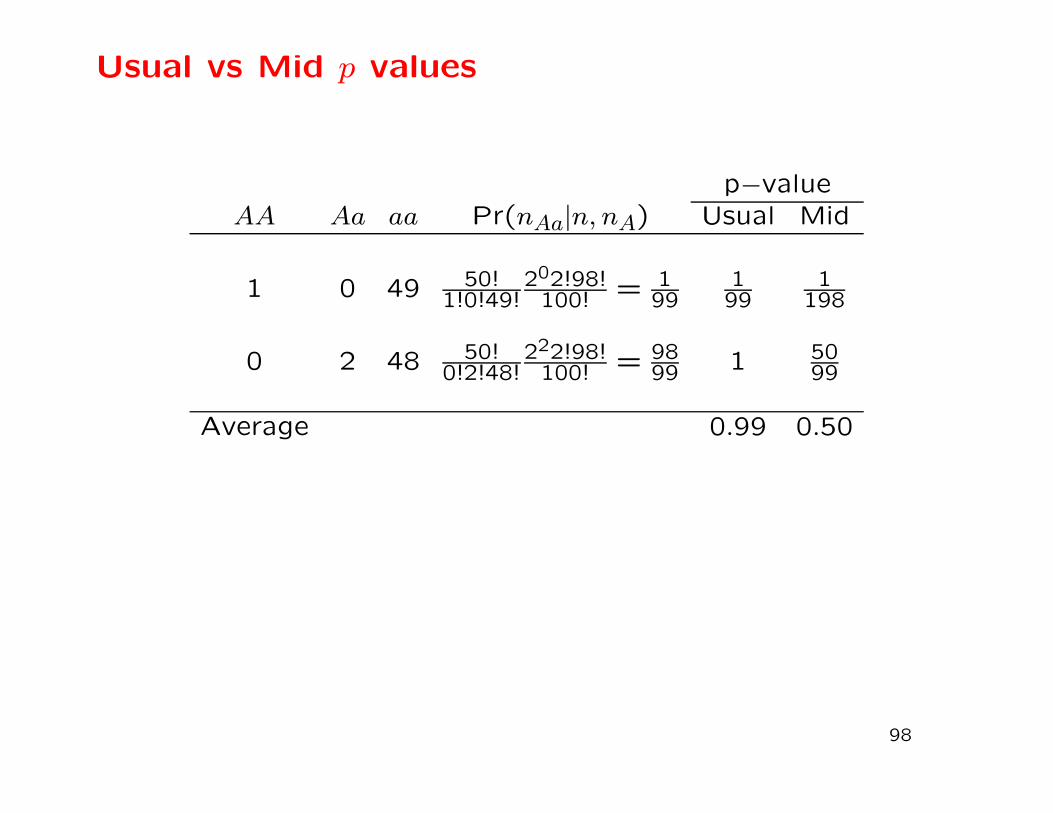
Usual vs Mid p values
p−valueAA Aa aa Pr(nAa|n, nA) Usual Mid
1 0 49 50!1!0!49!
202!98!100! = 1
99199
1198
0 2 48 50!0!2!48!
222!98!100! = 98
99 1 5099
Average 0.99 0.50
98

Usual vs Mid p values
p−valueAA Aa aa Pr(nAa|n, nA) Usual Mid
5 5 0 0.520 1.000 0.740
6 3 1 0.433 0.480 0.287
7 1 2 0.047 0.047 0.023
Average 0.730 0.510
99

Modified Exact HWE Test Example
For a sample of size n = 100 with minor allele frequency of 0.07,
there are 8 sets of possible genotype counts:
Exact Chi-square
nAA nAa naa Prob. Mid p-value X2 p-value
93 0 7 0.0000 0.0000∗ 100.00 0.0000∗92 2 6 0.0000 0.0000∗ 71.64 0.0000∗91 4 5 0.0000 0.0000∗ 47.99 0.0000∗90 6 4 0.0002 0.0002∗ 29.07 0.0000∗89 8 3 0.0051 0.0028∗ 14.87 0.0001∗88 10 2 0.0602 0.0353∗ 5.38 0.0204∗87 12 1 0.3209 0.2262 0.61 0.434886 14 0 0.6136 0.6832 0.57 0.4503
So, for a nominal 5% significance level, the actual significance
level is 0.0353 for an exact test that rejects when nAa ≤ 10 and
is 0.0204 for a chi-square test that also rejects when nAa ≤ 10.
100

Effect of Minor Allele Frequency
The minor allele frequency (MAF) in the previous example was
14/200 = 0.07. How does the exact test behave with other MAF
values?
In particular, what is the size of the rejection region for a nominal
value of α = 0.05? In other words, we decide to reject HWE
for any sample with a p-value of 0.05 or less, and we find the
total probability of all such datasets. We would hope that this
empirical significance level would be close to the nominal value,
but we find that it may not be.
101

na = 16 minor alleles
When the minor allele frequency is 0.08, for a nominal 5% signif-
icance level, the actual significance level is 0.0070 for an exact
test that rejects when nAa ≤ 10.
nAA nAa naa Pr(nAa|na) mid p −value
92 0 8 .0000 .000091 2 7 .0000 .000090 4 6 .0000 .000089 6 5 .0000 .000088 8 4 .0008 .000487 10 3 .0123 .007086 12 2 .0974 .061885 14 1 .3681 .294684 16 0 .5215 .7382
102
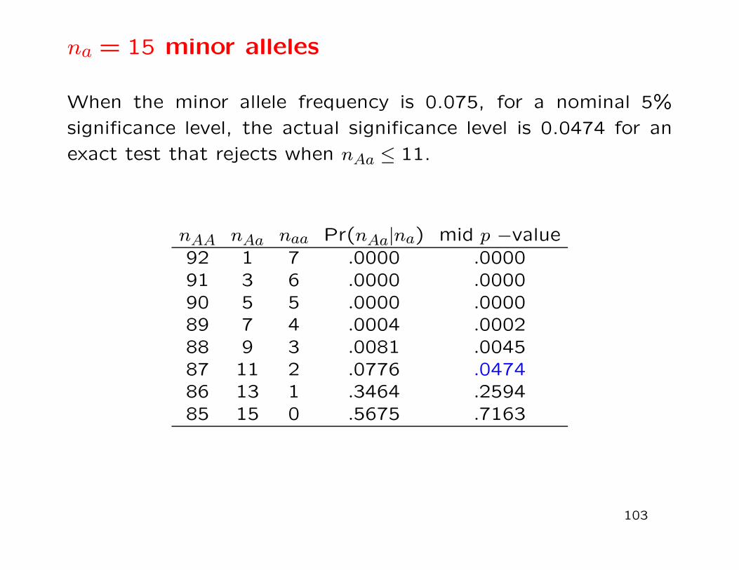
na = 15 minor alleles
When the minor allele frequency is 0.075, for a nominal 5%
significance level, the actual significance level is 0.0474 for an
exact test that rejects when nAa ≤ 11.
nAA nAa naa Pr(nAa|na) mid p −value
92 1 7 .0000 .000091 3 6 .0000 .000090 5 5 .0000 .000089 7 4 .0004 .000288 9 3 .0081 .004587 11 2 .0776 .047486 13 1 .3464 .259485 15 0 .5675 .7163
103

na = 13 minor alleles
When the minor allele frequency is 0.065, for a nominal 5%
significance level, the actual significance level is 0.0483 for an
exact test that rejects when nAa ≤ 9.
nAA nAa naa Pr(nAa|na) mid p −value
93 1 6 .0000 .000092 3 5 .0000 .000091 5 4 .0001 .000190 7 3 .0030 .003189 9 2 .0452 .048388 11 1 .2923 .340587 13 0 .6595 1.0000
104

na = 12 minor alleles
When the minor allele frequency is 0.06, for a nominal 5% signif-
icance level, the actual significance level is 0.0344 for an exact
test that rejects when nAa ≤ 8.
nAA nAa naa Pr(nAa|na) mid p −value
94 0 6 .0000 .000093 2 5 .0000 .000092 4 4 .0000 .000091 6 3 .0017 .001790 8 2 .0327 .018189 10 1 .2612 .165088 12 0 .7045 .2955
105

Graffelman and Moreno, 2013
106
Power of Exact Test
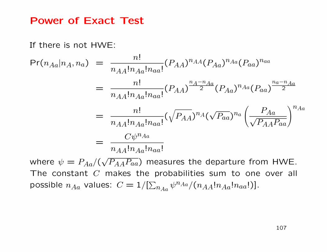
If there is not HWE:
Pr(nAa|nA, na) =n!
nAA!nAa!naa!(PAA)nAA(PAa)
nAa(Paa)naa
=n!
nAA!nAa!naa!(PAA)
nA−nAa2 (PAa)
nAa(Paa)na−nAa
2
=n!
nAA!nAa!naa!(√
PAA)nA(√Paa)
na
(
PAa√PAAPaa
)nAa
=CψnAa
nAA!nAa!naa!
where ψ = PAa/(√PAAPaa) measures the departure from HWE.
The constant C makes the probabilities sum to one over all
possible nAa values: C = 1/[∑
nAaψnAa/(nAA!nAa!naa!)].
107
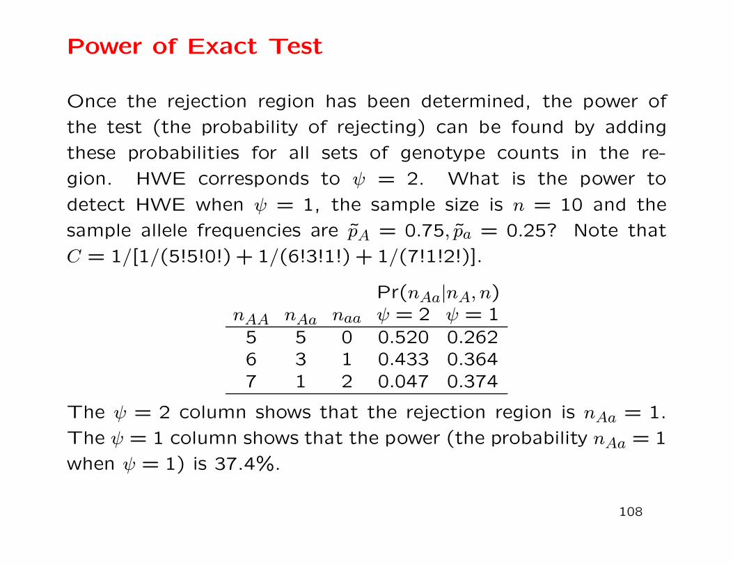
Power of Exact Test
Once the rejection region has been determined, the power of
the test (the probability of rejecting) can be found by adding
these probabilities for all sets of genotype counts in the re-
gion. HWE corresponds to ψ = 2. What is the power to
detect HWE when ψ = 1, the sample size is n = 10 and the
sample allele frequencies are pA = 0.75, pa = 0.25? Note that
C = 1/[1/(5!5!0!) + 1/(6!3!1!) + 1/(7!1!2!)].
Pr(nAa|nA, n)nAA nAa naa ψ = 2 ψ = 1
5 5 0 0.520 0.2626 3 1 0.433 0.3647 1 2 0.047 0.374
The ψ = 2 column shows that the rejection region is nAa = 1.
The ψ = 1 column shows that the power (the probability nAa = 1
when ψ = 1) is 37.4%.
108
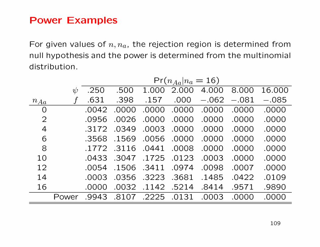
Power Examples
For given values of n, na, the rejection region is determined from
null hypothesis and the power is determined from the multinomial
distribution.
Pr(nAa|na = 16)ψ .250 .500 1.000 2.000 4.000 8.000 16.000
nAa f .631 .398 .157 .000 −.062 −.081 −.085
0 .0042 .0000 .0000 .0000 .0000 .0000 .00002 .0956 .0026 .0000 .0000 .0000 .0000 .00004 .3172 .0349 .0003 .0000 .0000 .0000 .00006 .3568 .1569 .0056 .0000 .0000 .0000 .00008 .1772 .3116 .0441 .0008 .0000 .0000 .0000
10 .0433 .3047 .1725 .0123 .0003 .0000 .000012 .0054 .1506 .3411 .0974 .0098 .0007 .000014 .0003 .0356 .3223 .3681 .1485 .0422 .010916 .0000 .0032 .1142 .5214 .8414 .9571 .9890
Power .9943 .8107 .2225 .0131 .0003 .0000 .0000
109
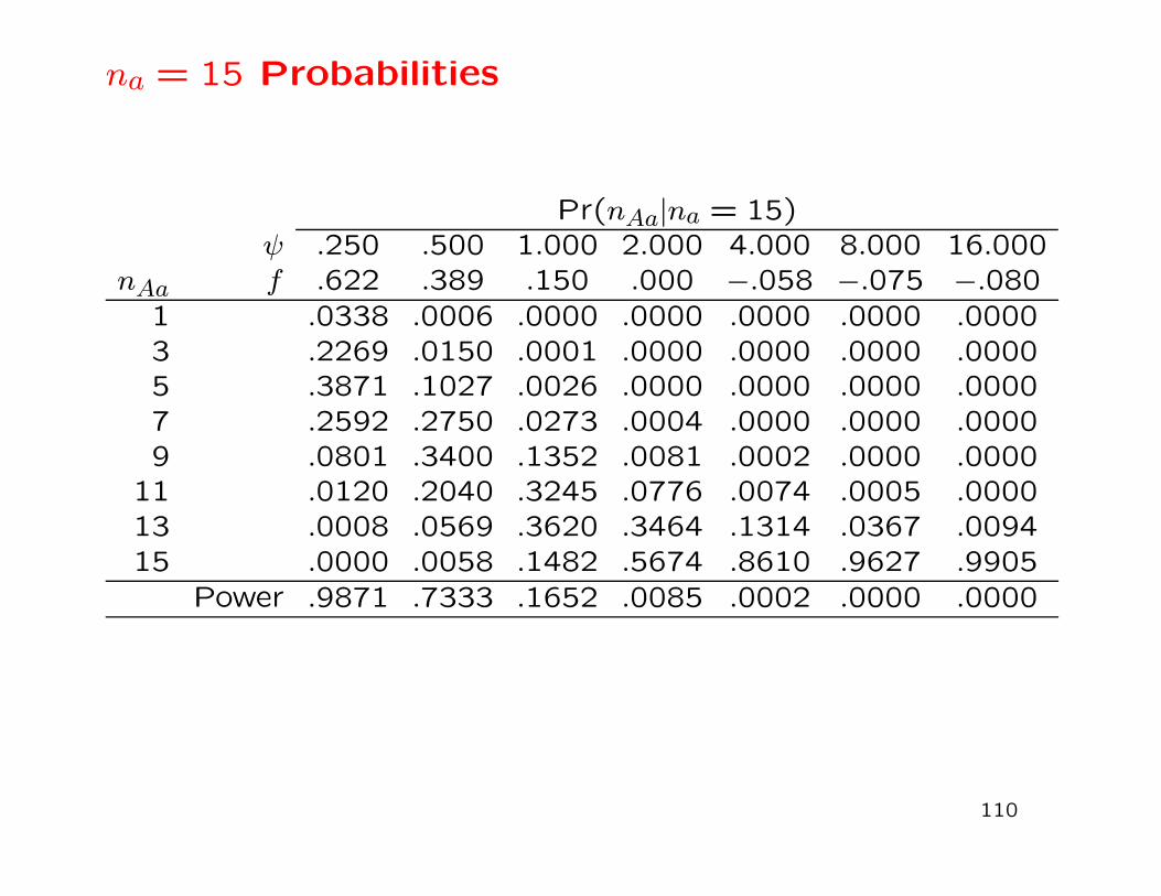
na = 15 Probabilities
Pr(nAa|na = 15)ψ .250 .500 1.000 2.000 4.000 8.000 16.000
nAa f .622 .389 .150 .000 −.058 −.075 −.080
1 .0338 .0006 .0000 .0000 .0000 .0000 .00003 .2269 .0150 .0001 .0000 .0000 .0000 .00005 .3871 .1027 .0026 .0000 .0000 .0000 .00007 .2592 .2750 .0273 .0004 .0000 .0000 .00009 .0801 .3400 .1352 .0081 .0002 .0000 .0000
11 .0120 .2040 .3245 .0776 .0074 .0005 .000013 .0008 .0569 .3620 .3464 .1314 .0367 .009415 .0000 .0058 .1482 .5674 .8610 .9627 .9905
Power .9871 .7333 .1652 .0085 .0002 .0000 .0000
110

na = 14 Probabilities
Pr(nAa|na = 14)ψ .250 .500 1.000 2.000 4.000 8.000 16.000
nAa f .613 .378 .143 .000 −.054 −.070 −.074
0 .0062 .0001 .0000 .0000 .0000 .0000 .00002 .1256 .0051 .0000 .0000 .0000 .0000 .00004 .3610 .0582 .0010 .0000 .0000 .0000 .00006 .3422 .2207 .0156 .0002 .0000 .0000 .00008 .1375 .3547 .1002 .0051 .0001 .0000 .0000
10 .0255 .2631 .2973 .0602 .0054 .0004 .000012 .0021 .0877 .3964 .3209 .1150 .0316 .008114 .0001 .0105 .1895 .6136 .8795 .9680 .9919
Power .9723 .6387 .1168 .0053 .0001 .0000 .0000
111

na = 13 Probabilities
Pr(nAa|na = 13)ψ .250 .500 1.000 2.000 4.000 8.000 16.000
nAa f .603 .366 .136 .000 −.050 −.065 −.068
1 .0479 .0012 .0000 .0000 .0000 .0000 .00003 .2786 .0275 .0003 .0000 .0000 .0000 .00005 .4004 .1583 .0080 .0001 .0000 .0000 .00007 .2169 .3430 .0696 .0030 .0001 .0000 .00009 .0508 .3216 .2611 .0452 .0038 .0003 .0000
11 .0051 .1301 .4225 .2923 .0994 .0269 .006913 .0002 .0183 .2383 .6595 .8967 .9728 .9931
Power .9947 .8516 .3391 .0483 .0039 .0003 .0000
112

na = 12 Probabilities
Pr(nAa|na = 12)ψ .250 .500 1.000 2.000 4.000 8.000 16.000
nAa f .592 .353 .128 .000 −.046 −.059 −.063
0 .0095 .0001 .0000 .0000 .0000 .0000 .00002 .1674 .0102 .0001 .0000 .0000 .0000 .00004 .4053 .0991 .0037 .0000 .0000 .0000 .00006 .3108 .3039 .0449 .0017 .0000 .0000 .00008 .0947 .3703 .2188 .0326 .0026 .0002 .0000
10 .0118 .1852 .4376 .2612 .0846 .0226 .005812 .0005 .0312 .2950 .7044 .9127 .9772 .9942
Power .9877 .7836 .2674 .0344 .0027 .0002 .0000
113

Graffelman and Moreno, 2013
114

Permutation Test
For large sample sizes and many alleles per locus, there are too
many genotypic arrays for a complete enumeration and a deter-
mination of which are the least probable 5% arrays.
A large number of the possible arrays is generated by permuting
the alleles among genotypes, and calculating the proportion of
these permuted genotypic arrays that have a smaller conditional
probability than the original data. If this proportion is small, the
Hardy-Weinberg hypothesis is rejected.
This procedure is not needed for SNPs with only 2 alleles. The
number of possible arrays is always less than bout half the sample
size.
115
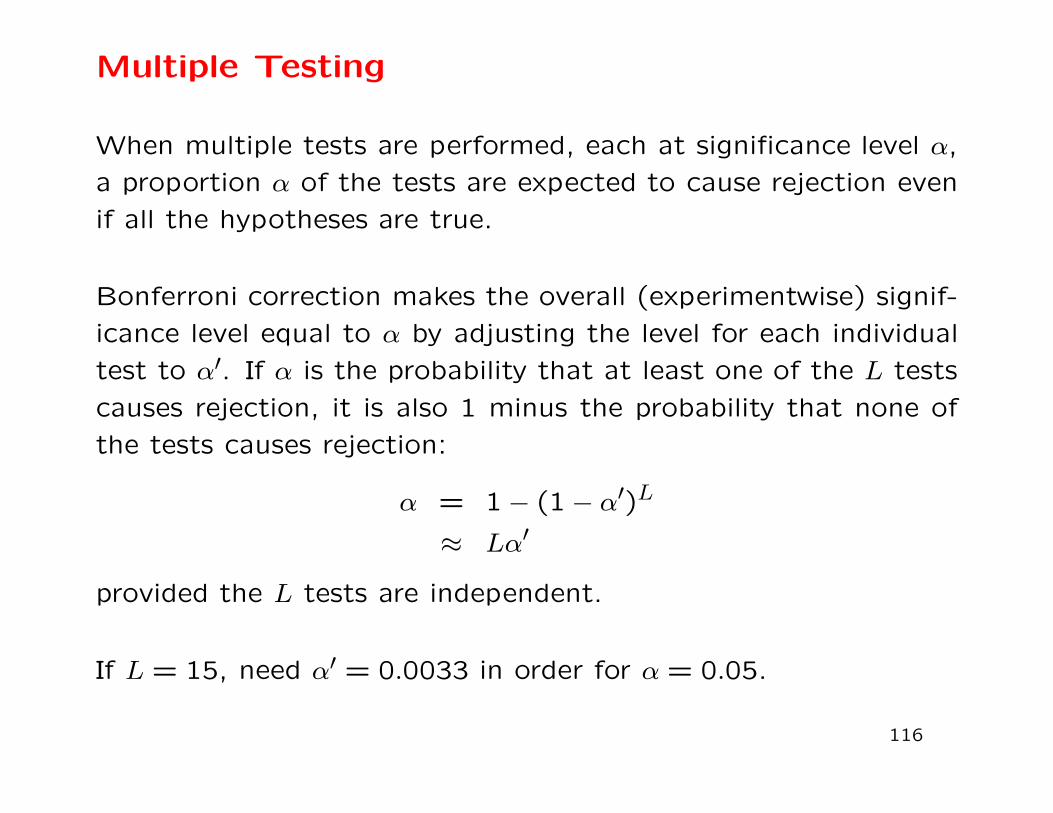
Multiple Testing
When multiple tests are performed, each at significance level α,
a proportion α of the tests are expected to cause rejection even
if all the hypotheses are true.
Bonferroni correction makes the overall (experimentwise) signif-
icance level equal to α by adjusting the level for each individual
test to α′. If α is the probability that at least one of the L tests
causes rejection, it is also 1 minus the probability that none of
the tests causes rejection:
α = 1 − (1 − α′)L
≈ Lα′
provided the L tests are independent.
If L = 15, need α′ = 0.0033 in order for α = 0.05.
116

QQ-Plots
An alternative approach to considering multiple-testing issues is
to use QQ-plots. If all the hypotheses being tested are true then
the resulting p-values are uniformly distributed between 0 and 1.
For a set of n tests, we would expect to see n evenly spread
p values between 0 an 1 e.g. 1/n,2/n, . . . , n/n. We plot the
observed p-values against these expected values: the smallest
against 1/n and the largest against 1. It is more convenient
to transform to − log10(p) to accentuate the extremely small p
values. The point at which the observed values start departing
from the expected values is an indication of “significant” values
in a way that takes into account the number of tests.
117

QQ-Plots
0 1 2 3 4
02
46
81
01
2
HWE Test: No SNP Filtering
−log10(p):Expected
−lo
g1
0(p
):O
bse
rve
d
The results for 9208 SNPs on human chromosome 1. Bonferroni
would suggest rejecting HWE when p ≤ 0.05/9205 = 5.4 × 10⁻⁶
or − log10(p) ≥ 5.3.
118

QQ-Plots
0 1 2 3 4
02
46
81
01
2
HWE Test: SNPs Filtered on Missingness
−log10(p):Expected
−lo
g1
0(p
):O
bse
rve
d
The same set of results as on the previous slide except now that
any SNP with any missing data was excluded. Now 7446 SNPs
and Bonferroni would reject if − log10(p) ≥ 5.2. All five outliers
had zero counts for the minor allele homozygote and at least 32
heterozygotes in a sample of size 50.
119
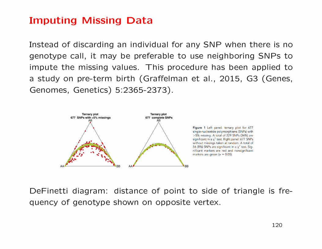
Imputing Missing Data
Instead of discarding an individual for any SNP when there is no
genotype call, it may be preferable to use neighboring SNPs to
impute the missing values. This procedure has been applied to
a study on pre-term birth (Graffelman et al., 2015, G3 (Genes,
Genomes, Genetics) 5:2365-2373).
DeFinetti diagram: distance of point to side of triangle is fre-
quency of genotype shown on opposite vertex.
120
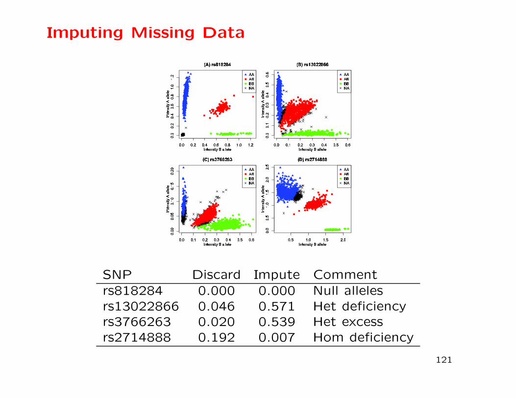
Imputing Missing Data
●●●●●●● ●●●●● ●●● ●●● ●●● ●● ●●
●●● ●●●● ●●●● ●●●● ● ●●● ●●
●● ●●●
● ● ● ●●●● ●●●●●● ●●●
� � � � � � � � � � � � � � � � � � � � �� ��� �� �� ��� �� �� �
� � � � � � � � � � �
� � � � � � � � � � � � �
! "# $"%& # '
( )** $* $●
+ ++ ,, ,- +
●●
●●
●●
●●
●●
●● ●
●●
●●
●●●●●● ● ●
●
●
●●●
● ● ●●
●●● ●●●
●● ●● ●● ●●
●
●
●●●●●
●● ●
●●
● ● ●●●
●●● ● ●●●
● ●● ●● ●
●
● ●●
● ●●● ●
●
●●
●●●
●●●●
●● ●●
● ● ● ●● ●●●
●● ●● ●●●●
●●
●
●●
●●●
●
●
●●● ●
● ●●
●
● ● ●●
●●●● ●●
●
●●●
●
● ●●●● ● ●● ●
●●●
●●
●
●
●●
●● ●●
●●
● ● ●●●
●
●●●
●●● ●●●
●●● ●
● ●●●●●
●●●● ●●
●●●●
●●●● ● ●●●●
●●●
●●● ●●● ●●●
●●
●●●● ●
. / . . / 0 . / 1 . / 2 . / 3 . / 4 . / 56 766 786 796 7:6 7;6 7<6 7=
> ? @ A B C D E F F G H H
I J K L J M N K O P Q R R L R L
S TU VTWX U Y
Z [\\ V\ V●
] ]] ^^ ^_ ]
●
●●●
●
●
●
●●
●
●●
●
●●
●●
●●
●
●
●
●
●
●●
●
●●●
●●
●
●
●
●
●●
●
●
●●
●
●●
●
●●●●●
●● ●
● ●
●●
●
●●
●●
●
●
●●
●
●
●●●● ●
●●
●
●●● ●●●
●
● ●●●
●
●●
●● ●●●
●
●●
●●
●●●●
●
●●
●
●●●
●●
●
●●
●
●
●●●
●
●
●
●●
●●
● ●●●
●
●
●
●●
●●
●
●●
●● ●
●●
●
●
●●
●
●●
●
●
●●●
●●● ●
● ●
●●
●
●●
●●
●
●●
●
●
●
●
●
●●●
●
● ● ●●
●
●
●
● ●
●● ●
● ●● ●
●
●
●●●●●●
●●
●●●●●
●● ●
●●
●●
●●
●
●
●
●
●
●●
●
●●
●●
●●●●
●●●
●
● ●
●
●
●●
●
●
●
●●
●
●
●● ●
●
●
●●
● ●
●
● ●●●●
●
●
●
●
●
●
●
●
●●
●●
●
●
●●●
●
●●●
●
●●
●
●
●
●●●
●●
●●
● ●
● ●●
●●
● ●●
●●
●●
●
●
●●
●●
●●
●●
●●
●
●●
●
●●
●●
●● ●
●●
●
●
●
●●
●● ●
●●
●
●
●
●
●●●
●
●●
● ●●
●●
●●
●
●●
●
●
● ●●
●
●
●●●
●●● ●
●
●●●● ●●
●●
●
●●
●●●
●
●
●
●
●●●
●
●●
●
●●
●●●
●
●
●
●●
●●
●
●●
●●
●
●
●
●
●●●
●●●
●
●
●
●
●
●
●●
●●
●
●
●
●
●●
●●●●
●
●
●
●●
●●
●●
●●●●●
●● ●
●
●● ●
●●
●
●
●
●
●
●
● ●●
●●
● ●
●●●
●
●
●●
●
●
●
●●●●
●
●
●
●●
●
●
●●
●
●● ●●
●
●●
●●
●
` a ` ` a b ` a c ` a d ` a e ` a f ` a gh ihhh ihjh ikhh ikjh ilh
m n o p q r s t t u t r
v w x y w z { x | } ~ � � y � y
� �� ���� � �
� ��� �� �●
� �� �� �� �
●●● ●●●●●● ● ●●●●● ●●●● ●● ●●●●
● ●● ●●●●●
●● ●●●● ● ●●● ●●●
● ●●●●● ●●● ●●● ● ●●● ●●●●●●●
� � � � � � � � � � � �� ��� ��� ��� ��� ��� ��
� � � � � � � � �
¡ ¢ £ ¤ ¢ ¥ ¦ £ § ¨ © ª ª ¤ ª ¤
« ¬ ®¬° ±² ³´´ ®´ ®
●
µ µµ ¶¶ ¶· µ
SNP Discard Impute Comment
rs818284 0.000 0.000 Null allelesrs13022866 0.046 0.571 Het deficiencyrs3766263 0.020 0.539 Het excessrs2714888 0.192 0.007 Hom deficiency
121
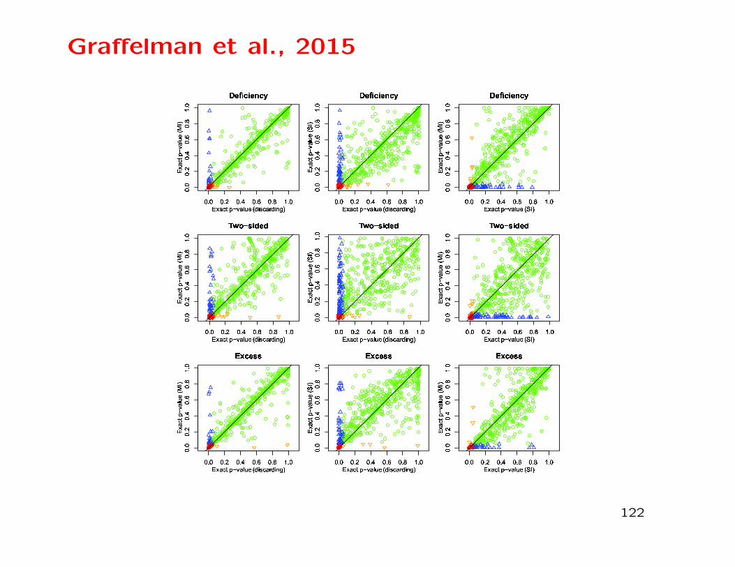
Graffelman et al., 2015
¸ ¹ ¸ ¸ ¹ º ¸ ¹ » ¸ ¹ ¼ ¸ ¹ ½ ¾ ¹ ¸¿ À¿¿ ÀÁ¿ À¿ Àÿ ÀÄÅ À¿
Æ Ç È É Ê É Ç Ë Ê Ì
Í Î Ï Ð Ñ Ò Ó Ô Ï Õ Ö × Ø Ù Ú Û Ð Ï Ü Ù Ú Ý Þ ß
à áâãä å
æçâè éêë ìí
î
ï ð ï ï ð ñ ï ð ò ï ð ó ï ð ô õ ð ïö ÷öö ÷øö ÷ùö ÷úö ÷ûü ÷ö
ý þ ÿ � � � þ � � �
� � � � � � � � � � � � � � � � � � � � �
� ���� �
���� !"# $
%
& ' & & ' ( & ' ) & ' * & ' + , ' &- .-- ./- .0- .1- .23 .-
4 5 6 7 8 7 5 9 8 :
; < = > ? @ A B = C D E F G H I
J KLMN O
PQLR STU VW
X
Y Z Y Y Z [ Y Z \ Y Z ] Y Z ^ _ Z Y` a`` ab` ac` ad` aef a`
g h i j k l m n m
o p q r s t u v q w x y z { | } r q ~ { | � � �
� ���� �
���� ��� ��
�
� � � � � � � � � � � � � � � � � �� ��� ��� ��� ��� ��� ��
� ¡ ¢ £ ¤ ¥ ¦ ¥
§ ¨ © ª « ¬ ® © ¯ ° ± ² ³ ´ µ ª © ¶ ³ ´ · ¸ ¹
º »¼½¾ ¿
ÀÁ¼Â ÃÄÅÆ Ç
È
É Ê É É Ê Ë É Ê Ì É Ê Í É Ê Î Ï Ê ÉÐ ÑÐÐ ÑÒÐ ÑÓÐ ÑÔÐ ÑÕÖ ÑÐ
× Ø Ù Ú Û Ü Ý Þ Ý
ß à á â ã ä å æ á ç è é ê ë ì í
î ïðñò ó
ôõðö ÷øù úû
ü
ý þ ý ý þ ÿ ý þ � ý þ � ý þ � � þ ý� ��� ��� ��� ��� � ��
� � � � �
� � � � � � � � � � � � � � � � � � � � � ! "
# $%&' (
)*%+ ,-. /0
1
2 3 2 2 3 4 2 3 5 2 3 6 2 3 7 8 3 29 :99 :;9 :<9 :=9 :>? :9
@ A B C D D
E F G H I J K L G M N O P Q R S H G T Q R U V W
X YZ[\ ]
^_Z` abcd e
f
g h g g h i g h j g h k g h l m h gn onn opn oqn orn ost on
u v w x y y
z { | } ~ � � � | � � � � � � �
� ���� �
���� ��� ��
�
122

HWE Test for X-linked Markers
Under HWE, allele frequencies in males and females should be
the same. Best to examine the difference when testing for HWE.
If a sample has nm males and nf females, and if the males have
mA,mB alleles of types A,B, and if females have fAA, fAB, fBBgenotypes AA,AB,BB, then the probability of the data, under
HWE, is
nA!nB!nm!nf !
mA!mB!fAA!fAB!fBB!nt!2fAB
where nt = nm + 2nf .
(Graffelman and Weir, 2016, Heredity 116:558-568).
123

Example: 10 males, 10 females, 6 A alleles
124

Graffelman and Weir, 2016. Possible Scenarios
125

Graffelman and Weir, 2016. Simulated Data
126
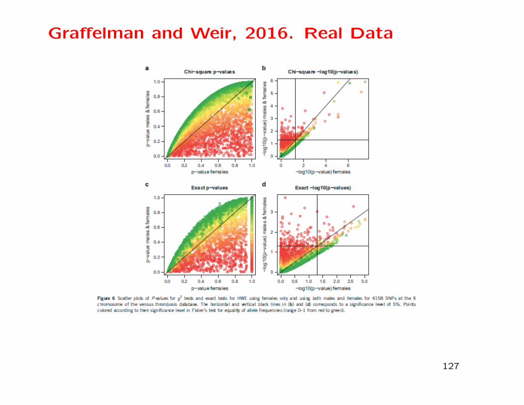
Graffelman and Weir, 2016. Real Data
127
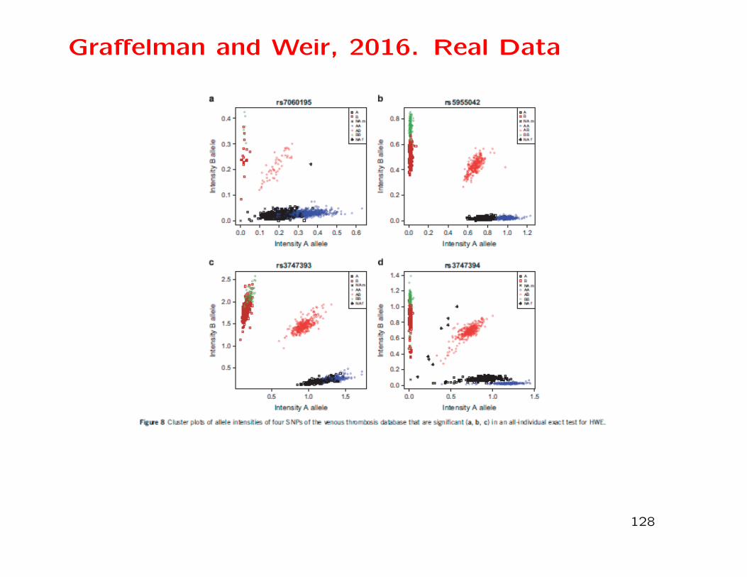
Graffelman and Weir, 2016. Real Data
128
Separate Male and Female Counts
The X-linked test can be extended to autosomal markers when
genotype counts are recorded separately for males and females.
129
SNV Data
Sequence-based variants have many low-frequency alleles that
are susceptible to effects of copy-number variation.
Recent survey of 1000Genomes data revealed more departures
from HWE than expected by chance, and many of these reflect
an apparent heterozygote excess. SNP-array data often shoe
HWE departures from heterozygote deficiency.
(Graffelman et al., 2017. Human Genetics 136:77-741.)
130

Whole Genome HWE Tests
131

MHC Region HWE Tests
Green: heterozygote deficiency. Red: heterozygote excess.
132

Copy Number Variants
JPT sample has 3.8% of variants in segmental duplications and
3% in simple tandem repeats. HWD rates 11 times higher in
these regions: reflecting sequencing problems due to multiple
copies of a variant, leading to heterozygote excess.
“Segmental duplications (SDs) are segments of DNA with near-
identical sequence.
A microsatellite is a tract of repetitive DNA in which certain
DNA motifs (ranging in length from 25 base pairs) are repeated,
typically 5-50 times.”
[Wikipedia]
133

Copy Number Variants
134

SNV-HWE Conclusions
Significant HWE results may indicate copy number variation -
excluding them may also exclude disease-associated variants.
NGS data have heterozygote excess, reflecting copy number vari-
ation.
SNP array data have heterozygote deficiency, reflecting null al-
leles.
135
Linkage Disequilibrium
This term reserved for association between pairs of alleles – one
at each of two loci.
When gametic data are available, could refer to gametic disequi-
librium.
When genotypic data are available, but gametes can be inferred,
can make inferences about gametic and non-gametic pairs of
alleles.
When genotypic data are available, but gametes cannot be in-
ferred, can work with composite measures of disequilibrium.
136

Linkage Disequilibrium
For alleles A and B are two loci, the usual measure of linkage
disequilibrium is
DAB = PAB − pApB
Whether or not this is zero does not provide a direct state-
ment about linkage between the two loci. For example, consider
marker YFM and disease DTD:
A N Total
+ 1 24 25YFM
− 0 75 75
Total 1 99 100
DA+ =1
100− 1
100
25
100= 0.0075, (maximum possible value)
137

Gametic Linkage Disequilibrium
For loci A, B define indicator variables x, y that take the value
1 for allele A,B and 0 for any other alleles. If gametes within
individuals are indexed by j, j = 1,2 then for expectations over
samples from the same population
E(xj) = pA, j = 1,2 , E(yj) = pB j = 1,2
E(x2j ) = pA, j = 1,2 , E(y2j ) = pB j = 1,2
E(x1x2) = PAA , E(y1y2) = PBB
E(x1y1) = PAB , E(x2y2) = PAB
The variances of xj, yj are pA(1− pA), pB(1− pB) for j = 1,2 and
the covariance and correlation coefficients for x and y are
Cov(x1, y1) = Cov(x2, y2) = PAB − pApB = DAB
Corr(x1, y1) = Corr(x2, y2) = DAB/√
[pA(1 − pA)pB(1 − pB)] = ρAB
138
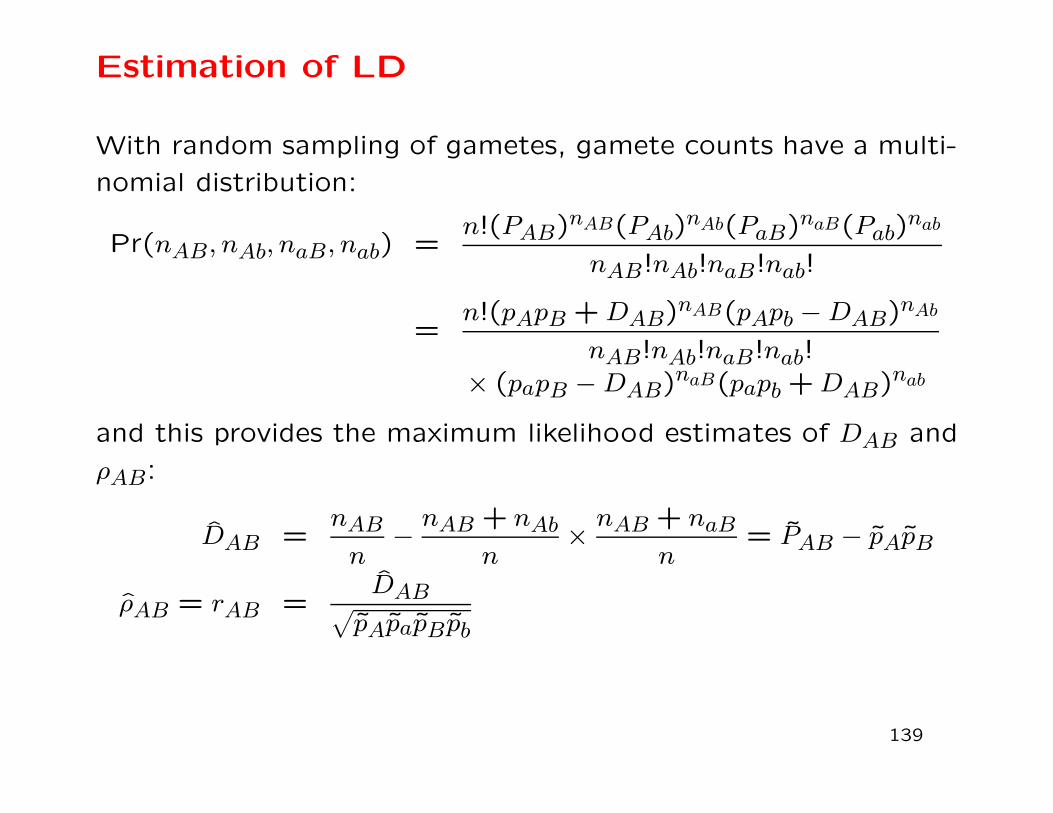
Estimation of LD
With random sampling of gametes, gamete counts have a multi-
nomial distribution:
Pr(nAB, nAb, naB, nab) =n!(PAB)nAB(PAb)
nAb(PaB)naB(Pab)nab
nAB!nAb!naB!nab!
=n!(pApB +DAB)nAB(pApb −DAB)nAb
nAB!nAb!naB!nab!
× (papB −DAB)naB(papb +DAB)nab
and this provides the maximum likelihood estimates of DAB and
ρAB:
DAB =nABn
− nAB + nAbn
× nAB + naBn
= PAB − pApB
ρAB = rAB =DAB
√
pApapBpb
139
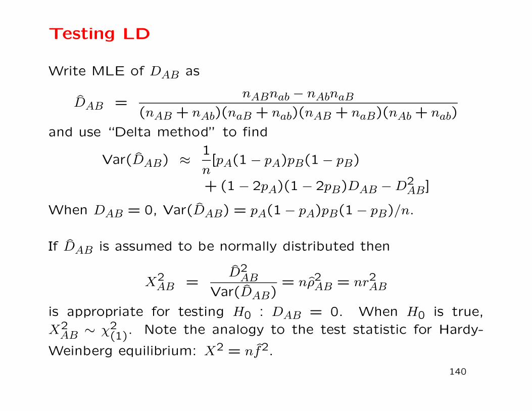
Testing LD
Write MLE of DAB as
DAB =nABnab − nAbnaB
(nAB + nAb)(naB + nab)(nAB + naB)(nAb + nab)
and use “Delta method” to find
Var(DAB) ≈ 1
n[pA(1 − pA)pB(1 − pB)
+ (1 − 2pA)(1 − 2pB)DAB −D2AB]
When DAB = 0, Var(DAB) = pA(1 − pA)pB(1 − pB)/n.
If DAB is assumed to be normally distributed then
X2AB =
D2AB
Var(DAB)= nρ2AB = nr2AB
is appropriate for testing H0 : DAB = 0. When H0 is true,
X2AB ∼ χ2
(1). Note the analogy to the test statistic for Hardy-
Weinberg equilibrium: X2 = nf2.
140

Goodness-of-fit Test
The test statistic for the 2 × 2 table
nAB nAb nAnaB nab nanB nb n
has the value
X2 =n(nABnab − nAbnaB)2
nAnanBnb
For DTD/YFM example, X2 = 3.03. This is not statistically
significant, even though disequilibrium was maximal.
141

Composite Disequilibrium
When genotypes are scored, it is often not possible to distinguish
between the two double heterozygotes AB/ab and Ab/aB, so that
gametic frequencies cannot be inferred.
Under the assumption of random mating, in which genotypic fre-
quencies are assumed to be the products of gametic frequencies,
it is possible to estimate gametic frequencies with the EM algo-
rithm. To avoid making the random-mating assumption, how-
ever, it is possible to work with a set of composite disequilibrium
coefficients.
142

Composite Disequilibrium
Although the separate digenic frequencies pAB (one gamete) and
pA,B (two gametes) cannot be observed, their sum can be since
pAB = PABAB +1
2PABAb +
1
2PABaB +
1
2PABab
pA,B = PABAB +1
2PABAb +
1
2PABaB +
1
2PAbaB
pAB + pA,B = 2PABAB + PABAb + PABaB +PABab + PAbaB
2
Digenic disequilibrium is measured with a composite measure
∆AB defined as
∆AB = pAB + pA,B − 2pApB
= DAB +DA,B
which is the sum of the gametic (DAB = pAB−pApB) and nonga-
metic (DA,B = pA,B − pApB) coefficients.
143

Composite Disequilibrium
If the counts of the nine genotypic classes are
BB Bb bbAA n1 n2 n3Aa n4 n5 n6aa n7 n8 n9
the count for pairs of alleles in an individual being A and B,
whether received from the same or different parents, is
nAB = 2n1 + n2 + n4 +1
2n5
and the MLE for ∆ is
∆AB =1
nnAB − 2pApB
144

Composite Linkage Disequilibrium
For loci A, B define indicator variables x, y that take the value
1 for allele A,B and 0 for any other alleles. If gametes within
individuals are indexed by j, j = 1,2 then for expectations over
samples from the same population
E(xj) = pA, j = 1,2 , E(yj) = pB j = 1,2
E(x2j ) = pA, j = 1,2 , E(yj) = pB j = 1,2
E(x1x2) = PAA , E(y1y2) = PBB
E(x1y1) = PAB , E(x2y2) = PAB
E(x1y2) = PA,B , E(x2y1) = PA,B
Write
DA = PAA − p2A , DB = PBB − p2B
DAB = PAB − pApB , DA,B = PA,B − pApB
∆AB = DAB +DA,B
145
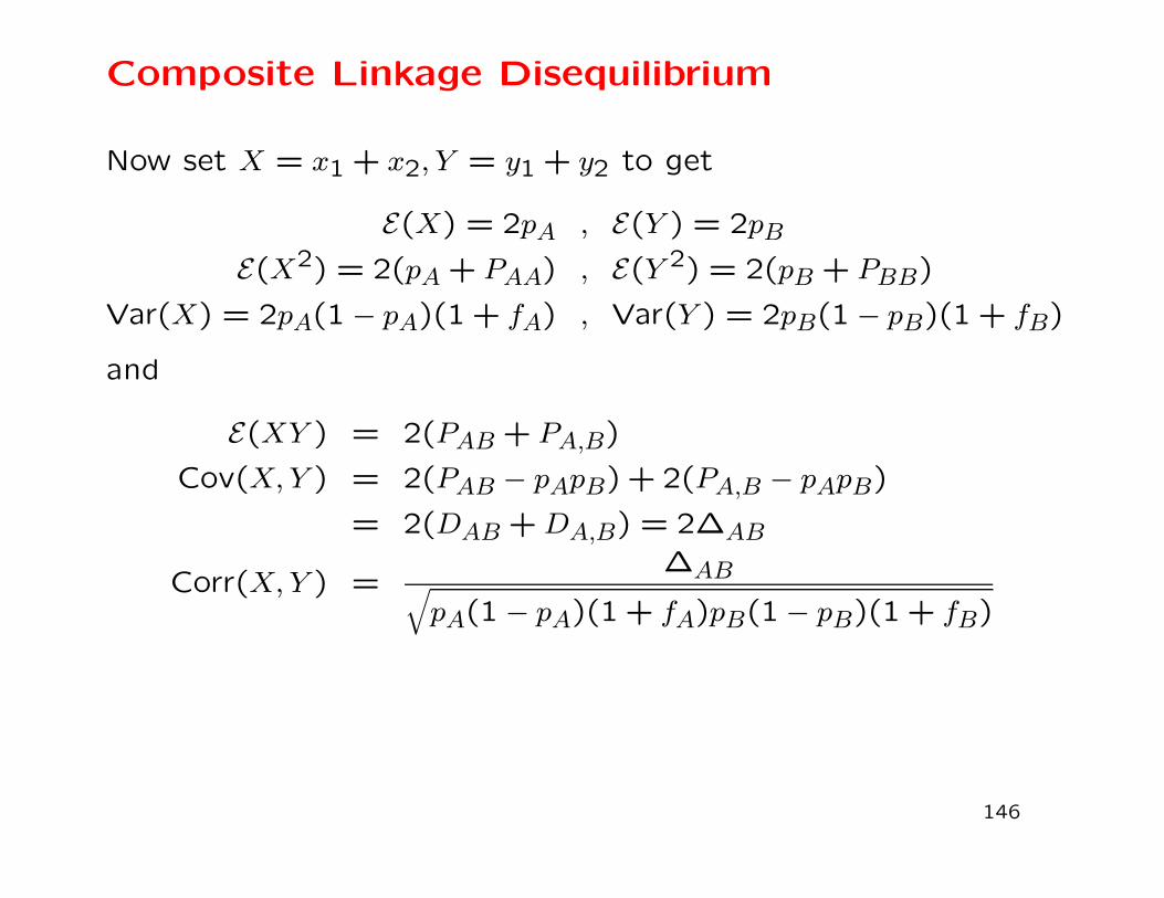
Composite Linkage Disequilibrium
Now set X = x1 + x2, Y = y1 + y2 to get
E(X) = 2pA , E(Y ) = 2pB
E(X2) = 2(pA + PAA) , E(Y 2) = 2(pB + PBB)
Var(X) = 2pA(1 − pA)(1 + fA) , Var(Y ) = 2pB(1 − pB)(1 + fB)
and
E(XY ) = 2(PAB + PA,B)
Cov(X,Y ) = 2(PAB − pApB) + 2(PA,B − pApB)
= 2(DAB +DA,B) = 2∆AB
Corr(X,Y ) =∆AB
√
pA(1 − pA)(1 + fA)pB(1 − pB)(1 + fB)
146

Composite Linkage Disequilibrium
∆AB = nAB/n− 2pApB
where
nAB = 2nAABB + nAABb + nAaBB +1
2nAaBb
This does not require phased data.
By analogy to the gametic linkage disequilibrium result, a test
statistic for ∆AB = 0 is
X2AB =
n∆2AB
pA(1 − pA)(1 + fA)pB(1 − pB)(1 + fB)
This is assumed to be approximately χ2(1)
under the null hypoth-
esis.
147

Example
For the data
BB Bb bb Total
AA nAABB = 5 nAABb = 3 nAAbb = 2 nAA = 10Aa nAaBB = 3 nAaBb = 2 nAabb = 0 nAa = 5aa naaBB = 0 naaBb = 0 naabb = 0 naa = 0
Total nBB = 8 nBb = 5 nbb = 2 n = 15
nAB = 2 × 5 + 3 + 3 +1
2(2) = 17
nA = 25, pA = 5/6
nB = 21, pB = 7/10
148

Example
The estimated composite disequilibrium coefficient is
∆AB =17
15− 2
25
30
21
30= − 1
30= −0.033
Previous work on EM algorithm estimated pAB as 16/30 so
DAB =16
30− 25
30
21
30= − 1
20= −0.050
149

Multi-locus Disequilibria: Entropy
It is difficult to describe associations among alleles at several
loci. One approach is based on information theory.
For a locus with sample frequencies pu for alleles Au the entropy
is
HA = −∑
upu ln(pu)
For independent loci, entropies are additive: if haplotypes AuBv
have sample frequencies Puv the two-locus entropy is
HAB = −∑
u
∑
vPuv ln(Puv) = −
∑
u
∑
vpupv[ln(pu) + ln(pv)] = HA +HB
so if HAB 6= HA + HB there is evidence of dependence. This
extends to multiple loci.
150

Conditional Entropy
If the entropy for a multi-locus profile A is HA then the condi-
tional probability of another locus B, given A, is HB|A = HAB −HA.
In performing meaningful calculations for Y-STR profiles, this
suggests choosing a set of loci by an iterative procedure. First
choose locus L1 with the highest entropy. Then choose locus L2
with the largest conditional entropy H(L2|L1). Then choose L3
with the highest conditional entropy with the haplotype L1L2,
and so on.
151

Conditional Entropy: YHRD Data
Added Entropy Added EntropyMarker Single Multi Cond. Marker Single Multi Cond.YS385ab 4.750 4.750 4.750 DYS481 2.962 6.972 2.222DYS570 2.554 8.447 1.474 DYS576 2.493 9.318 0.871DYS458 2.220 9.741 0.423 DYS389II 2.329 9.906 0.165DYS549 1.719 9.999 0.093 DYS635 2.136 10.05 0.053DYS19 2.112 10.08 0.028 DYS439 1.637 10.10 0.024DYS533 1.433 10.11 0.010 DYS456 1.691 10.12 0.006GATAH4 1.512 10.12 0.005 DYS393 1.654 10.13 0.003DYS448 1.858 10.13 0.002 DYS643 2.456 10.13 0.002DYS390 1.844 10.13 0.002 DYS391 1.058 10.13 0.002
This table shows that the most-discriminating loci may not con-
tribute to the most-discriminating haplotypes. Furthermore, there
is little additional discriminating power from Y-STR haplotypes
beyond 10 loci.
152
Population Structure and Relatedness
153
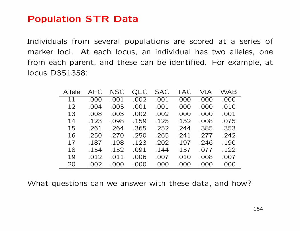
Population STR Data
Individuals from several populations are scored at a series of
marker loci. At each locus, an individual has two alleles, one
from each parent, and these can be identified. For example, at
locus D3S1358:
Allele AFC NSC QLC SAC TAC VIA WAB11 .000 .001 .002 .001 .000 .000 .00012 .004 .003 .001 .001 .000 .000 .01013 .008 .003 .002 .002 .000 .000 .00114 .123 .098 .159 .125 .152 .008 .07515 .261 .264 .365 .252 .244 .385 .35316 .250 .270 .250 .265 .241 .277 .24217 .187 .198 .123 .202 .197 .246 .19018 .154 .152 .091 .144 .157 .077 .12219 .012 .011 .006 .007 .010 .008 .00720 .002 .000 .000 .000 .000 .000 .000
What questions can we answer with these data, and how?
154

HapMap III SNP Data
SampleCode Population Description sizeASW African ancestry in Southwest USA 142CEU Utah residents with Northern and Western 324
European ancestry from CEPH collectionCHB Han Chinese in Beijing, China 160CHD Chinese in Metropolitan Denver, Colorado 140GIH Gujarati Indians in Houston, Texas 166JPT Japanese in Tokyo, Japan 168LWK Luhya in Webuye, Kenya 166MXL Mexican ancestry in Los Angeles, California 142MKK Maasai in Kinyawa, Kenya 342TSI Toscani in Italia 154YRI Yoruba in Ibadan, Nigeria 326
155
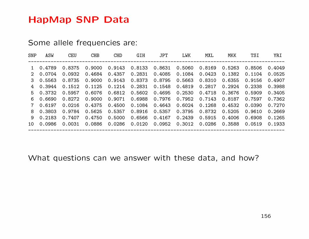
HapMap SNP Data
Some allele frequencies are:
SNP ASW CEU CHB CHD GIH JPT LWK MXL MKK TSI YRI
------------------------------------------------------------------------------------------1 0.4789 0.8375 0.9000 0.9143 0.8133 0.8631 0.5060 0.8169 0.5263 0.8506 0.40492 0.0704 0.0932 0.4684 0.4357 0.2831 0.4085 0.1084 0.0423 0.1382 0.1104 0.0525
3 0.5563 0.8735 0.9000 0.9143 0.8373 0.8795 0.5663 0.8310 0.6355 0.9156 0.49074 0.3944 0.1512 0.1125 0.1214 0.2831 0.1548 0.4819 0.2817 0.2924 0.2338 0.3988
5 0.3732 0.5957 0.6076 0.6812 0.5602 0.4695 0.2530 0.4718 0.3676 0.5909 0.34056 0.6690 0.8272 0.9000 0.9071 0.6988 0.7976 0.7952 0.7143 0.8187 0.7597 0.7362
7 0.6197 0.0216 0.4375 0.4500 0.1084 0.4643 0.6024 0.1268 0.4532 0.0390 0.72708 0.3803 0.9784 0.5625 0.5357 0.8916 0.5357 0.3795 0.8732 0.5205 0.9610 0.26699 0.2183 0.7407 0.4750 0.5000 0.6566 0.4167 0.2439 0.5915 0.4006 0.6908 0.1265
10 0.0986 0.0031 0.0886 0.0286 0.0120 0.0952 0.3012 0.0286 0.3588 0.0519 0.1933------------------------------------------------------------------------------------------
What questions can we answer with these data, and how?
156

Questions of Interest
• How much genetic variation is there? (animal conservation)
• How much migration (gene flow) is there between popula-
tions? (molecular ecology)
• How does the genetic structure of populations affect tests for
linkage between genetic markers and human disease genes?
(human genetics)
• How should the evidence of matching marker profiles be
quantified? (forensic science)
• What is the evolutionary history of the populations sampled?
(evolutionary genetics)
157
Statistical Analysis
Possible to approach these data from purely statistical viewpoint.
Could test for differences in allele frequencies among populations.
Could use various multivariate techniques to cluster populations.
These analyses may not answer the biological questions.
158

Genetic Analysis: Frequencies of Allele Au
Population 1 Population r
p1u . . .
πu
pru
Among samples of ni alleles from population i: counts for allele u
follow a binomial distribution with mean piu and variance nipiu(1−piu). Sample allele frequencies piu have expected values piu and
variances piu(1 − piu)/ni.
Among replicates of population i: piu values follow a Beta dis-
tribution with mean πu and variance πu(1 − πu)θi.
159

Beta distribution: Theoretical
The beta probability density is proportional to pv−1(1 − p)w−1
and can take a variety of shapes.
0.0 0.4 0.8
0.6
1.0
1.4
v=1,w=1
0.0 0.4 0.8
0.0
1.0
v=2,w=2
0.0 0.4 0.8
0.0
1.0
2.0
v=4,w=4
0.0 0.4 0.8
0.0
1.0
2.0
v=2,w=1
0.0 0.4 0.8
01
23
4
v=4,w=1
0.0 0.4 0.8
01
23
4
v=1,w=4
0.0 0.4 0.8
1.0
1.3
1.6
v=0.9,w=0.9
0.0 0.4 0.8
24
68
u=0.5,w=0.5
0.0 0.4 0.8
01
02
5
u=0.5,w=4
160
Beta distribution: Experimental
The beta distribution is suggested by a Drosophila experiment
with 107 replicate populations of size 16, starting with all het-
erozygotes, by P. Buri (Evolution 10:367, 1956).
161
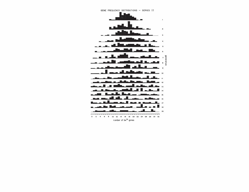

What is θ?
Two ways of thinking about θ.
It measures the extra degree of relatedness of individuals because
they belong to the same population. We think of this reflecting
long-term evolutionary history, but can use the same logic for
people related because they are in the same family: first cousins
have a θ value of 0.0625.
θ also helps to measure the variance of allele frequencies over
populations.
These notes rest on “A unified characterization of population
structure and relatedness” by Weir and Goudet, to be published
in the August 2017 issue of Genetics. It was made available on
May 26, 2017 in Genetics Early Online.
https://doi.org/10.1534/genetics.116.198424
162

What is θ?
Population i
BB
BB
BBBM
��������
θi
. . .
HHHHHHHHHY
���������*
θii′
Population i′
BB
BB
BBBM
��������
θi′
θ’s are statements about pairs of alleles: the probabilities the
pairs are identical by descent.
θW is average of the within-population coancestries θi.
θB is average of the between-population-pair coancestries θii′.
163

Predicted Values of the θ’s: Pure Drift
Our estimation procedure for the θ’s holds for all evolutionary
scenarios, but the theoretical values of the θ’s do depend on the
history of the sampled populations.
In the case of pure drift, where population i has constant size Niand there is random mating, t generations after the population
began drifting from an ancestral population in which θi = 0
θi(t) = 1 −(
1 − 1
2Ni
)t
If t is small relative to large Ni’s, θi(t) ≈ t/(2Ni), and θW (t) ≈
t/(2Nh) where Nh is the harmonic mean of the Ni.
164
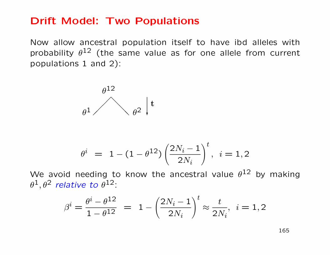
Drift Model: Two Populations
Now allow ancestral population itself to have ibd alleles with
probability θ12 (the same value as for one allele from current
populations 1 and 2):
?
t
θ12
��
���
@@
@@@θ1 θ2
θi = 1 − (1 − θ12)
(
2Ni − 1
2Ni
)t
, i = 1,2
We avoid needing to know the ancestral value θ12 by making
θ1, θ2 relative to θ12:
βi =θi − θ12
1 − θ12= 1 −
(
2Ni − 1
2Ni
)t
≈ t
2Ni, i = 1,2
165

Two populations: drift, migration, mutation
Population 1Time t
?
Drift
N1
Population 2
?
Drift
N2
HHHHHHHHHHHHHHHHHHHHj
���������������������
Migration
m1 m2
Population 1Time t+ 1 Population 2
There is also a probability µ that an allele mutates to a new type.
166
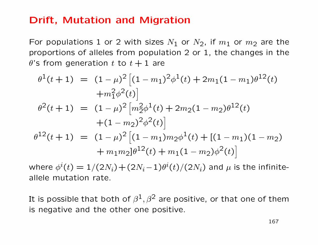
Drift, Mutation and Migration
For populations 1 or 2 with sizes N1 or N2, if m1 or m2 are the
proportions of alleles from population 2 or 1, the changes in the
θ’s from generation t to t+ 1 are
θ1(t+ 1) = (1 − µ)2[
(1 −m1)2φ1(t) + 2m1(1 −m1)θ
12(t)
+m21φ
2(t)]
θ2(t+ 1) = (1 − µ)2[
m22φ
1(t) + 2m2(1 −m2)θ12(t)
+(1 −m2)2φ2(t)
]
θ12(t+ 1) = (1 − µ)2[
(1 −m1)m2φ1(t) + [(1 −m1)(1 −m2)
+m1m2]θ12(t) +m1(1 −m2)φ
2(t)]
where φi(t) = 1/(2Ni)+(2Ni−1)θi(t)/(2Ni) and µ is the infinite-
allele mutation rate.
It is possible that both of β1, β2 are positive, or that one of them
is negative and the other one positive.
167
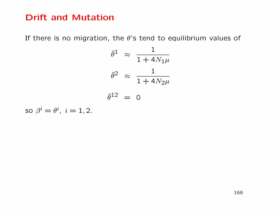
Drift and Mutation
If there is no migration, the θ’s tend to equilibrium values of
θ1 ≈ 1
1 + 4N1µ
θ2 ≈ 1
1 + 4N2µ
θ12 = 0
so βi = θi, i = 1,2.
168

Drift, Mutation and Migration
The θ’s are non-negative, but one of the β’s may be negative.
0 2000 6000 10000
0.0
0.4
0.8
mu=0; m1=m2=0
Generation
Th
eta N=100
N=10000
0 2000 6000 10000
0.0
0.4
0.8
mu=0.001; m1=m2=0
GenerationT
he
ta N=100N=10000
0 2000 6000 10000
0.0
0.4
0.8
mu=.001; m1=0.001,m2=0
Generation
Th
eta Theta1
Theta2Theta12
Drift Only Drift and Mutation Drift, Mutationand Migration
β1, β2 > 0 β1, β2 > 0 β1 > 0, β2 < 0
169
Genotypes vs Alleles
So far we have ignored individual genotypic structure, leading
to an analysis of population allele frequencies as opposed to
genotypic frequencies.
θi is the probability two alleles drawn randomly from population i
are ibd, and θii′is the probability an allele drawn randomly from
population i is ibd to an allele drawn from population i′.
Within population i, we define θijj as the probability that two
alleles drawn randomly from individual j are ibd, and θijj′ as the
probability that allele drawn randomly from individual j is ibd to
an allele from individual j′.
170
Coancestry vs Inbreeding
The coancestry of individuals j, j′ in population i is the probability
an allele from j is ibd to an allele from j′. This is θijj′.
The inbreeding of individual j in population i is the probability
the two alleles in that individual are ibd. Write this as F ij .
Two alleles drawn from individual j are equally likely to be the
same allele or different alleles:
θijj =1
2
(
1 + F ij
)
171

Predicted Values: Path Counting
A↙ ↘
... ...↘ ↓ ↓ ↙
X Y↘ ↙
I
Identify the path linking the parents of I to their common an-
cestor(s).
172
Path Counting
If the parents X,Y of an individual I have ancestor A in common,
and if there are n individuals (including X,Y, I) in the path linking
the parents through A, then the inbreeding coefficient of I, or
the coancestry of X and Y , is
FI = θXY =
(
1
2
)n(1 + FA)
If there are several ancestors, this expression is summed over all
the ancestors.
173
Average Coancestries
The average over all pairs of distinct individuals, j 6= j′, of the
coancestries θijj′ is written as θiS. The average of this over pop-
ulations is θS. These are probabilities for individuals.
When there is random mating and Hardy-Weinberg equilibrium in
a population, any pair of distinct alleles in a population (within
or between individuals) is equivalent and then the average ibd
probability for all these pairs is written as θiW , where W means
within populations. The average over populations is θW . These
are probabilities for distinct alleles.
The ibd probability for any allele from population i and any allele
from population i′ is θii′
B , where B means between populations.
Averaging over all pairs of distinct populations gives θB.
174

Relative Inbreeding: FIS
For population i, the inbreeding coefficient for individual j, rela-
tive to the identity of pairs of alleles between individuals in that
population, is
βij =F ij − θiS
1 − θiS
The average over individuals within this population is the population-
specific F iIS, and it compares within-indivdual ibd to between-
individual ibd in the same population. It is the quantity being
addressed by Hardy-Weinberg testing in population i.
If the reference set of alleles is for pairs of individuals within
populations, averaged over populations, then the average relative
inbreeding coefficient is βIS = (F I − θS)/(1− θS) where F I is the
average of F ij over individuals j and populations i. It is generally
called FIS.
175

Relative Inbreeding: FIT
For population i, the inbreeding coefficient for individual j, rela-
tive to the identity of pairs of alleles from different populations
averaged over all pairs of populations, is
βij =F ij − θB
1 − θB
The average over individuals within this population is the population-
specific F iIT . The average of these over all populations is the
total inbreeding coefficient FIT = (F I − θB)/(1 − θB).
176

Relative Coancestry: FST for Individuals
For population i, the coancestry of individuals j, j′ relative to the
coancestry for all pairs of individuals in that population is
βijj′ =θijj′ − θiS
1 − θiSand these average zero over all pairs of individuals in the popu-
lation.
If the reference set is all pairs of alleles, one from each of two
populations,
βijj′ =θijj′ − θB
1 − θB
The average βiST over all pairs of individuals in population i is
the population-specific F iST , and averaging this over populations
gives the global FST = (θS − θB)/(1 − θB). It is the ibd proba-
bility between individuals within populations relative to the ibd
probability between populations.
177

FIS, FIT , FST for Individuals
When individuals are distinguished:
(1 − FIT) = (1 − FIS)(1 − FST)
FIS =FIT − FST1 − FST
This classic result also holds for population-specific values
(1 − F iIT) = (1 − F iIS)(1 − F iST)
F iIS =F iIT − F iST1 − F iST
178
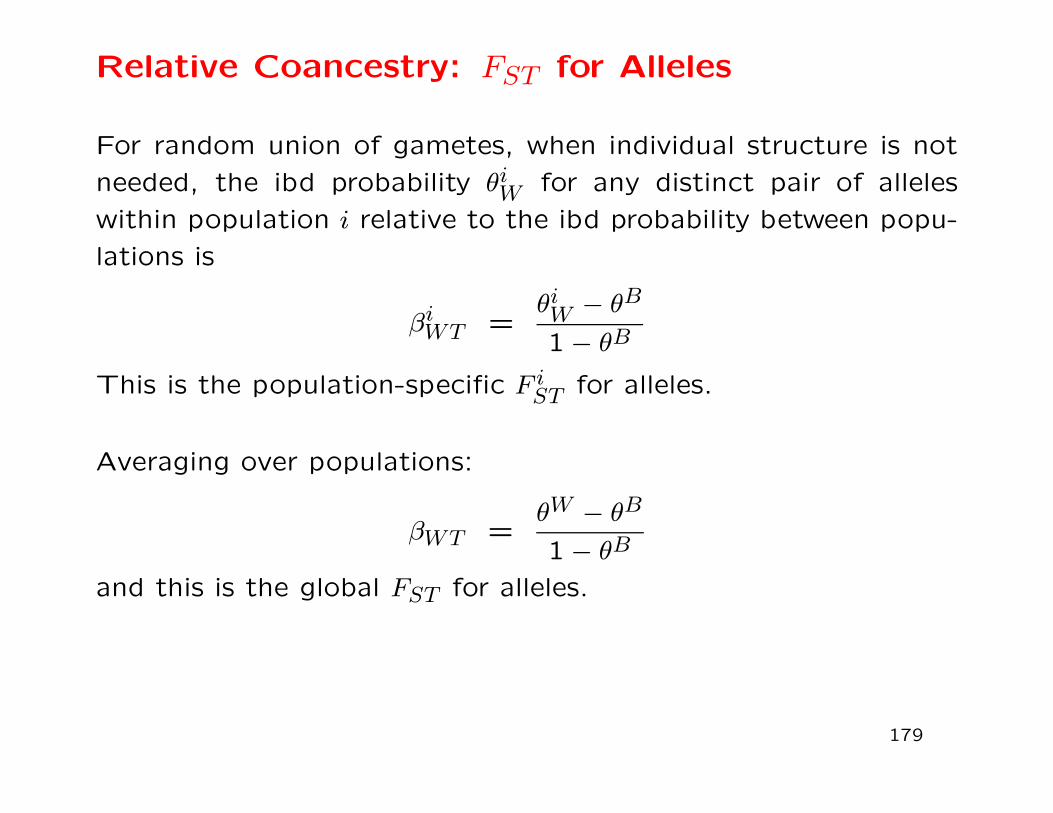
Relative Coancestry: FST for Alleles
For random union of gametes, when individual structure is not
needed, the ibd probability θiW for any distinct pair of alleles
within population i relative to the ibd probability between popu-
lations is
βiWT =θiW − θB
1 − θB
This is the population-specific F iST for alleles.
Averaging over populations:
βWT =θW − θB
1 − θB
and this is the global FST for alleles.
179

Estimation of β’s
Now that the various measures for individuals and populations
are defined, it is straightforward to estimate them from genotypic
or allelic data.
For any allele we set its indicator variable xu to be 1 if that
allele is of type u and to be 0 if it is not of type u. Then the
expected value of xu or of x2u is the allele frequency πu. For any
two distinct alleles, the expected value of the product of their
xu’s is π2u + πu(1 − πu)θ where θ is the ibd probability for those
two alleles.
We examine pairs of alleles to see whether or not they are the
same type: i.e. they match. When two alleles match, the prod-
uct of their indicators is 1 and the expected value of the propor-
tion of matching pairs depends on θ. We manipulate matching
proportions to give estimates of the θ’s.
180

Allelic Matching Proportions for Individuals
For individual j in population i the proportion of its distinct alleles
that match is either 0 or 1. It is convenient to work with allele
dosages Xiju for the number of its alleles that are of type u and
write the matching proportion as
M ij =
1
2
∑
uXiju(X
iju − 1)
For biallelic SNPs, the reference allele dosage is Xij (with values
0, 1 or 2) and the matching proportion is (Xij − 1)2 - this is still
0 or 1. The expected value over replicates of the population is
E(M ij) = MT + (1 −MT )F ij
where MT =∑
u π2u is unknown.
We avoid having to know MT by estimating F ij relative to either
pairs of alleles from different individuals (i.e. coancestry) in the
same population, or pairs of alleles from different populations.
181

Allelic Matching Proportions for Pairs of Individ-uals
The proportion of pairs of alleles, one from individual j and
one from j′ in population i that match is 0, 0.5 or 1. These
proportions can be expressed in terms of allele dosages
M ijj′ =
1
4
∑
uXijuX
ij′u
For biallelic SNPs, with reference allele dosages Xij the matching
proportion is [1 + (Xij − 1)(Xi
j′ − 1)]/2 - this is still 0, 0.5 or 1.
The expected value over replicates of the population is
E(M ijj′) = MT + (1 −MT )θijj′
Averaging over all pairs of individuals, the observed and expected
matching proportion are
M iS =
1
ni(ni − 1)
ni∑
j=1
ni∑
j′ 6=j
M ijj′ , E(M i
S) = MT + (1 −MT )θiS
182

Within-population Inbreeding Estimates
The inbreeding coefficient of an individual can be estimated as its
allelic matching proportion relative to the matching proportion
for pairs of individuals in the same population:
βij =M ij − M i
S
1 − M iS
, E(βij) =F ij − θiS
1 − θiS
These estimates may be negative.
Averaging over individuals, with M iI =
∑nij=1 M
ij/ni,
βiIS = F iIS =M iI − M i
S
1 − M iS
, E(βiI) = F iIS =F iI − θiS1 − θiS
If there are data from several populations, we may use MS as
the average within-population coancestry, averaged over popu-
lations, so that inbreeding is estimated relative to this average.
183
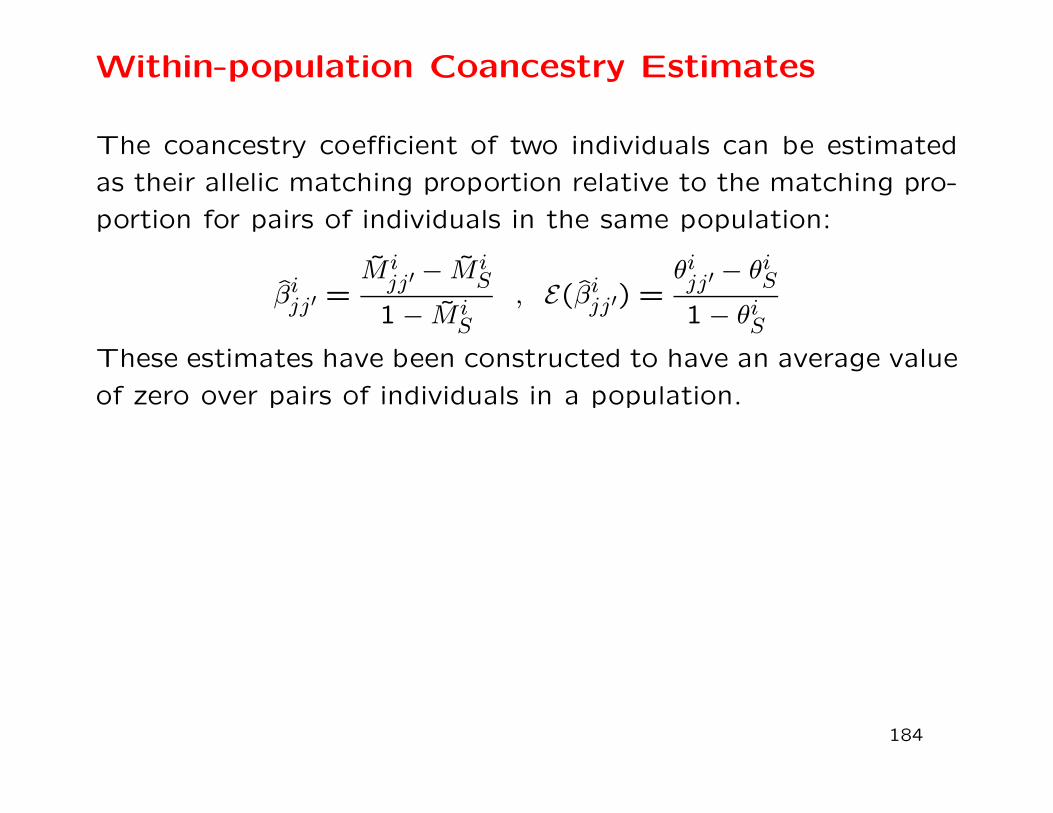
Within-population Coancestry Estimates
The coancestry coefficient of two individuals can be estimated
as their allelic matching proportion relative to the matching pro-
portion for pairs of individuals in the same population:
βijj′ =M ijj′ − M i
S
1 − M iS
, E(βijj′) =θijj′ − θiS
1 − θiS
These estimates have been constructed to have an average value
of zero over pairs of individuals in a population.
184

Comparison with Standard Inbreeding and Coances-try Estimates
For SNPs, omitting population superscripts, we estimate inbreed-
ing and coancestry by
βj =(Xj − 1)2 − MS
1 − MS, E(βj) =
Fj − θS
1 − θS
βjj′ =12[1 + (Xj − 1)(Xj′ − 1)] − MS
1 − MS, E(βjj′) =
θjj′ − θS
1 − θS
where MS =∑nj=1
∑nj′ 6=j Mjj′/[n(n − 1)].
Standard estimates use sample allele frequencies p =∑nj=1X
ij/(2n):
βj =(Xj − 2p)2
2p(1 − p)− 1
βjj′ =(Xj − 2p)(Xj′ − 2p)
4p(1 − p)
185

Standard estimate expectations
The standard estimates have expectations that depend on the
inbreeding and coancestry coefficients of all members of the sam-
ple. This can result in pairs of individuals having β rankings that
differ from their θ rankings.
E(βjj′) =(θjj′ − ψj − ψj′ + θS) − 1
n(θjj + θj′j′ − ψj − ψj′ − FS + θS)
(1 − θS)− 1n(FS − θS)
where FS =∑nj=1 θjj/n is the average of all within-individual
coancestries (1 + Fj)/2, ψj =∑nj′=1,j′ 6=j θjj′/(n − 1) is the av-
erage coancestry of individual j to all other individuals, and
θS =∑nj=1ψj/n.
When j = j′, we have θjj = (1 + Fj)/2.
186
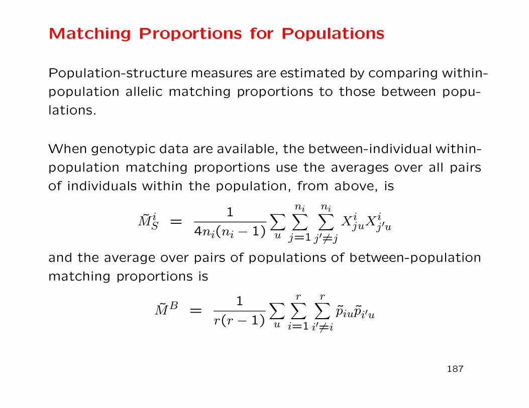
Matching Proportions for Populations
Population-structure measures are estimated by comparing within-
population allelic matching proportions to those between popu-
lations.
When genotypic data are available, the between-individual within-
population matching proportions use the averages over all pairs
of individuals within the population, from above, is
M iS =
1
4ni(ni − 1)
∑
u
ni∑
j=1
ni∑
j′ 6=j
XijuX
ij′u
and the average over pairs of populations of between-population
matching proportions is
MB =1
r(r − 1)
∑
u
r∑
i=1
r∑
i′ 6=i
piupi′u
187

Genotype-based FST Estimates
The within- and between-population matching proportions for
genotypic data set have expectations
E(M iS) = MT + (1 −MT )θiS
E(MB) = MT + (1 −MT )θB
so the population-specific, genotype-based, FST estimate is
βiST = F iST =M iS − MB
1 − MB
Averaging over populations, the genotype-based global FST es-
timate is
βST = FST =MS − MB
1 − MB
188

SNP-genotype-based FST Estimates
For SNPs, with allele dosages X:
M iS =
1
2ni(ni − 1)
ni∑
j=1
ni∑
j′ 6=j
[1 + (Xij − 1)(Xi
j′ − 1)]
MB =1
r(r − 1)
r∑
i=1
r∑
i′ 6=i
[pipi′ + (1 − pi)(1 − pi′)]
189

Allele-based Matching Proportions within Popu-lations
When the genotypic structure of data is ignored, or not known,
allelic data can be used to estimate FST .
If alleles from ni individuals are observed for population i, the ob-
served matching proportion of allele pairs within this population
is
M iW =
1
2ni(2ni − 1)
∑
u
2ni∑
j=1
2ni∑
j′ 6=j
xjuxj′u
=2ni
2ni − 1
∑
up2iu − 1
2ni − 1
where piu is the sample frequency for allele u for this population.
The expected value of this over replicates of the population is
E(M iW ) = MT + (1 −MT )θiW
where MT =∑
u π2u.
190
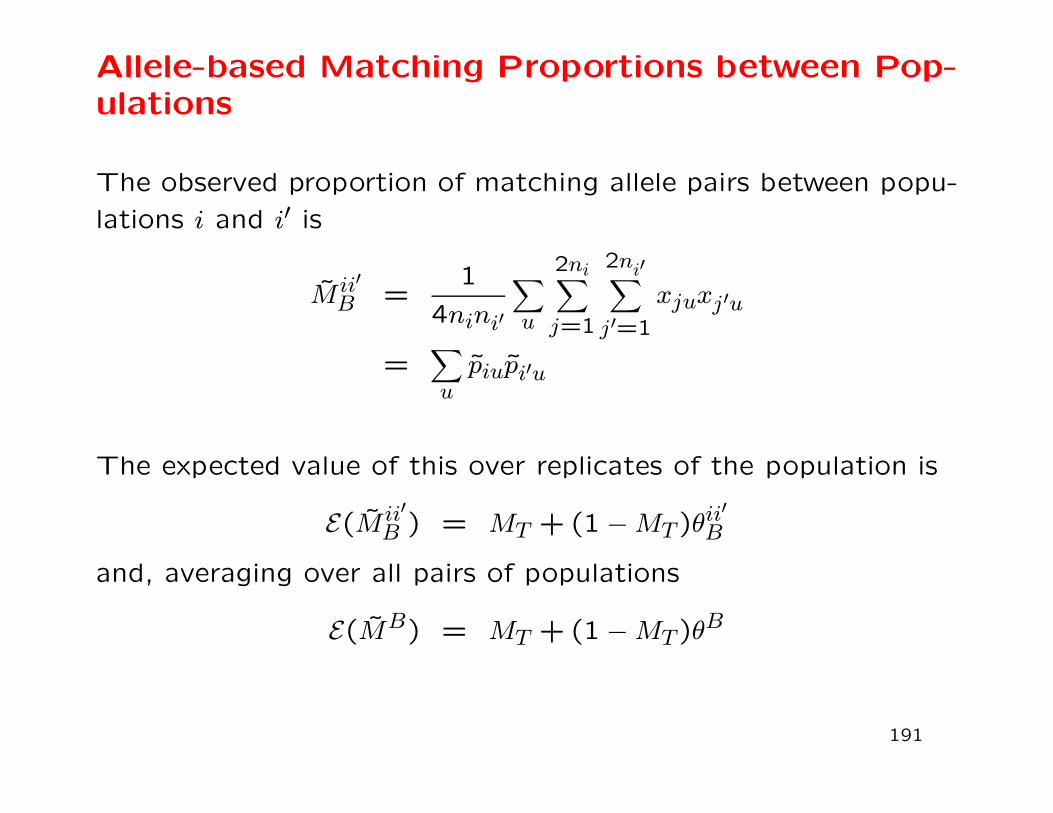
Allele-based Matching Proportions between Pop-ulations
The observed proportion of matching allele pairs between popu-
lations i and i′ is
M ii′B =
1
4nini′
∑
u
2ni∑
j=1
2ni′∑
j′=1
xjuxj′u
=∑
upiupi′u
The expected value of this over replicates of the population is
E(M ii′B ) = MT + (1 −MT )θii
′B
and, averaging over all pairs of populations
E(MB) = MT + (1 −MT )θB
191

Allele-based Estimate of FST
We avoid having to know MT by considering allele-pair matching
within a population relative to the allele-pair matching between
pairs of populations:
βiWT = F iST =M iW − MB
1 − MB
and this has expected value F iWT = (θiW − θB)/(1 − θB) which is
the population-specific value.
Average over populations:
FWT = βWT =MW − MB
1 − MB
and this has expected value FWT = (θW − θB)/(1 − θB) which is
the global value.
192

Simple Computing Equations for FST
For large sample sizes and r populations:
M iW ≈
∑
up2iu
MW =1
r
r∑
i=1
M iW =
∑
up2u +
r − 1
r
∑
us2u
where pu =∑ri=1 piu/r is the mean allele frequency over popula-
tions, and s2u =∑ri=1(piu − pu)2/(r − 1) is the variance of allele
frequencies over populations.
For all sample sizes:
M ii′B =
∑
upiupi′u
MB =1
r(r − 1)
r∑
i=1
r∑
i′ 6=i
M ii′B =
∑
up2u − 1
r
∑
us2u
193

Simple Allele-based Estimates for FST
The allele-based population-specific estimates are
F iWT =
∑
u[(p2iu − p2u) + s2u]
∑
u[pu(1 − pu) + 1rs
2u
The corresponding global estimates are
FWT =
∑
u s2u
∑
u[pu(1 − pu) + 1rs
2u]
194

SNP-allele-based Estimates for FST
For SNPs with two alleles, write pi for the reference allele sample
frequency for population i. In this case,∑
u pu(1− pu) = 2p(1− p)where p =
∑ri=1 pi/r, and
∑
u s2u = 2s2 where s2 =
∑ri=1(p −
p)2/(r − 1).
The population-specific estimates are
F iWT =p2i − p2 + s2
p(1 − p) + 1rs
2
The global estimates are
FWT =s2
p(1 − p) + 1rs
2
195

SNP-allele-based Estimates of FST for Two Pop-ulations
For SNP studies with two populations, with reference allele sam-
ple frequencies p1, p2, p = (p1 + p2)/2 and s2 = (p1 − p2)2/2.
The population-specific estimates are
β1WT = F1
WT =(p1 − p2)(2p1 − 1)
p1(1 − p2) + p2(1 − p1)
β2WT = F2
WT =(p2 − p1)(2p2 − 1)
p1(1 − p2) + p2(1 − p1)
One of these two may be negative.
The global estimate is
βWT = FWT =(p1 − p2)
2
p1(1 − p2) + p2(1 − p1)
This must be positive.
196

Multiple Loci
The unweighted estimators for locus l are of the form
βl =Numeratorl
Denominatorl
There are several ways to combine estimates over loci. Here,
we weight by the denominators: With several loci, these can be
extended to
β =
∑
lNumeratorl∑
lDenominatorl
and these estimate β if each locus has the same value of the θ’s.
Otherwise they estimate a weighted average of the different θ
values, where the weights are functions of the allele frequencies
at the loci in the sum.
197
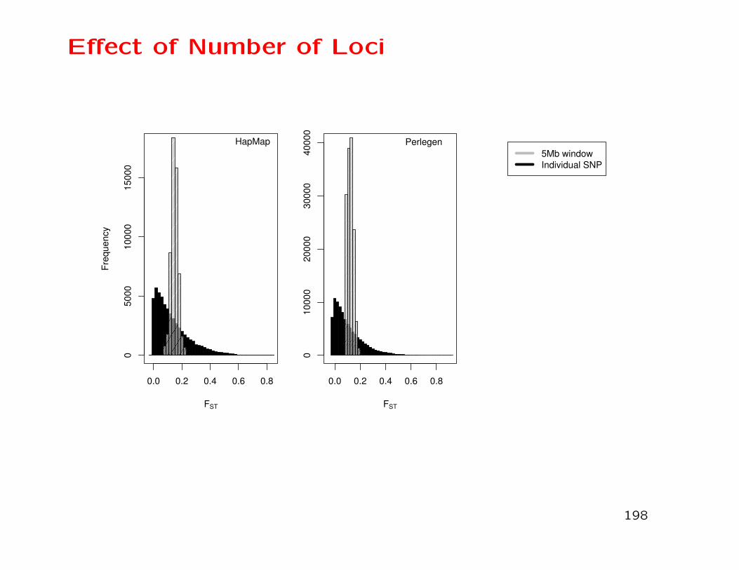
Effect of Number of Loci
FST
Fre
qu
en
cy
0.0 0.2 0.4 0.6 0.8
05
00
01
00
00
15
00
0
HapMap
FST
0.0 0.2 0.4 0.6 0.8
01
00
00
20
00
03
00
00
40
00
0
Perlegen
5Mb window
Individual SNP
198
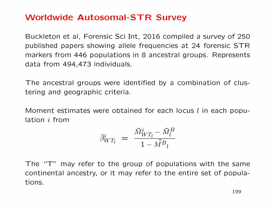
Worldwide Autosomal-STR Survey
Buckleton et al, Forensic Sci Int, 2016 compiled a survey of 250
published papers showing allele frequencies at 24 forensic STR
markers from 446 populations in 8 ancestral groups. Represents
data from 494,473 individuals.
The ancestral groups were identified by a combination of clus-
tering and geographic criteria.
Moment estimates were obtained for each locus l in each popu-
lation i from
βiWTl=
M iWTl
− MBl
1 − MBl
The “T” may refer to the group of populations with the same
continental ancestry, or it may refer to the entire set of popula-
tions.
199

STR Survey: β Values for Groups and Loci
Geographic RegionLocus Africa AusAb Asian Cauc Hisp IndPK NatAm Poly Aver.CSF1PO 0.003 0.002 0.008 0.008 0.002 0.007 0.055 0.026 0.011D1S1656 0.000 0.000 0.000 0.002 0.003 0.000 0.000 0.000 0.011D2S441 0.000 0.000 0.002 0.003 0.021 0.000 0.000 0.000 0.020D2S1338 0.009 0.004 0.011 0.017 0.013 0.003 0.023 0.005 0.031D3S1358 0.004 0.010 0.009 0.006 0.012 0.040 0.079 0.001 0.025D5S818 0.002 0.013 0.009 0.008 0.014 0.018 0.044 0.007 0.029D6S1043 0.000 0.000 0.000 0.000 0.000 0.000 0.000 0.000 0.016D7S820 0.004 0.021 0.010 0.007 0.007 0.046 0.030 0.005 0.026D8S1179 0.003 0.007 0.012 0.006 0.002 0.031 0.020 0.008 0.019D10S1248 0.000 0.000 0.000 0.002 0.004 0.000 0.000 0.000 0.007D12S391 0.000 0.000 0.000 0.003 0.020 0.000 0.000 0.000 0.010D13S317 0.015 0.016 0.013 0.008 0.014 0.025 0.050 0.014 0.038D16S539 0.007 0.002 0.015 0.006 0.009 0.005 0.048 0.004 0.021D18S51 0.011 0.012 0.014 0.006 0.004 0.010 0.033 0.003 0.018D19S433 0.009 0.001 0.009 0.010 0.014 0.000 0.022 0.014 0.023D21S11 0.014 0.012 0.013 0.007 0.006 0.023 0.067 0.018 0.021D22S1045 0.000 0.000 0.007 0.001 0.000 0.000 0.000 0.000 0.015FGA 0.002 0.009 0.012 0.004 0.007 0.016 0.021 0.006 0.013PENTAD 0.008 0.000 0.012 0.012 0.002 0.017 0.000 0.000 0.022PENTAE 0.002 0.000 0.017 0.006 0.003 0.012 0.000 0.000 0.020SE33 0.000 0.000 0.012 0.001 0.000 0.000 0.000 0.000 0.004TH01 0.022 0.001 0.022 0.016 0.018 0.014 0.071 0.017 0.071TPOX 0.019 0.087 0.016 0.011 0.007 0.018 0.064 0.031 0.035VWA 0.009 0.007 0.017 0.007 0.012 0.022 0.028 0.005 0.023All Loci 0.006 0.014 0.010 0.007 0.008 0.018 0.043 0.011 0.022
200

Coancestry is relative, not absolute
The new relative coancestry estimates have been applied to 1000Genomes data, and compared to standard estimates, shown onnext slide.
For the whole world, all 26 populations, as reference the betaestimates show a relatively narrow range of values within eachAfrican population (AFR) and lower African values than in therest of the world, as expected from our understanding of highergenetic diversity within African than non-African populationsfrom the migration history of modern humans. This pattern wasnot shown by the standard estimates - those estimates showedhigher coancestry among African individuals than among non-Africans.
The wide plots for the Admixed American populations (AMR)reflect the admixture within those populations, with greater re-latedness reflecting more ancestral commonality. When eachcontinental group is used as a reference, all populations showlow coancestry, except for the admixed AMR.
201

Coancestry is relative, not absolute
Top row: Whole world reference. Bottom row: Continental group reference.
Beta estimates Standard estimates
Chromosome 22 data from 1000 Genomes.
Continents (left to right): AFR, SAS, EUR, EAS, AMR
Populations (l to r):AFR: ACB, ASW, ESN, GWD, LWK, MSL, YRI;SAS: BEB, GIH, ITU, PJL, STU; EUR: CEU, FIN, GBR, IBS, TSI;EAS: CDX, CHB, CHS, JPT; AMR: KHV, CLM, MXL, PEL, PUR
202

FST is relative, not absolute
Using data from the 1000 genomes, using 1,097,199 SNPs on
chromosome 22.
For the samples originating from Africa, there is a larger FWT ,
βWT = 0.013, with Africa as a reference set than there is, βWT =
−0.099, with the world as a reference set. African populations
tend to be more different from each other on average than do
any two populations in the world on average.
The opposite was found for East Asian populations: there is a
smaller FWT , βWT = 0.013 with East Asia as a reference set
than there is, βWT = 0.225 with the world as a reference set.
East Asian populations are more similar to each other than are
any pair of populations in the world.
203

βWT in LCT Region: 3 Populations
100 120 140 160 180
0.0
0.1
0.2
0.3
0.4
0.5
0.6
0.7
HapMap III Chromosome 2
Position
Be
ta−
W
LCT
CEU
CHB
YRI
204

βWT in LCT Region: 11 Populations
100 120 140 160 180
0.0
0.1
0.2
0.3
0.4
0.5
0.6
0.7
HapMap III Chromosome 2
Position
Be
ta−
W
LCT
CEU
MKK
Other
205
MKK Population
“The Maasai are a pastoral people in Kenya and Tanzania, whose
traditional diet of milk, blood and meat is rich in lactose, fat
and cholesterol. In spite of this, they have low levels of blood
cholesterol, and seldom suffer from gallstones or cardiac diseases.
Analysis of HapMap 3 data using Fixation Index (Fst) identified
genomic regions and single nucleotide polymorphisms (SNPs)
as strong candidates for recent selection for lactase persistence
and cholesterol regulation in 143156 founder individuals from the
Maasai population in Kinyawa, Kenya (MKK). The strongest
signal identified by all three metrics was a 1.7 Mb region on
Chr2q21. This region contains the gene LCT (Lactase) involved
in lactase persistence.”
Wagh et al., PLoS One 7: e44751, 2012
206

Weir & Cockerham 1984 Model
W&C assumed all populations have equal evolutionary histories
(θi = θ, all i) and are independent (θii′= 0, all i′ 6= i), and
they worked with overall allele frequencies that were weighted by
sample sizes
pu =1
∑
i ni
∑
i
nipiu
If θ = 0, these weighted means have minimum variance.
207
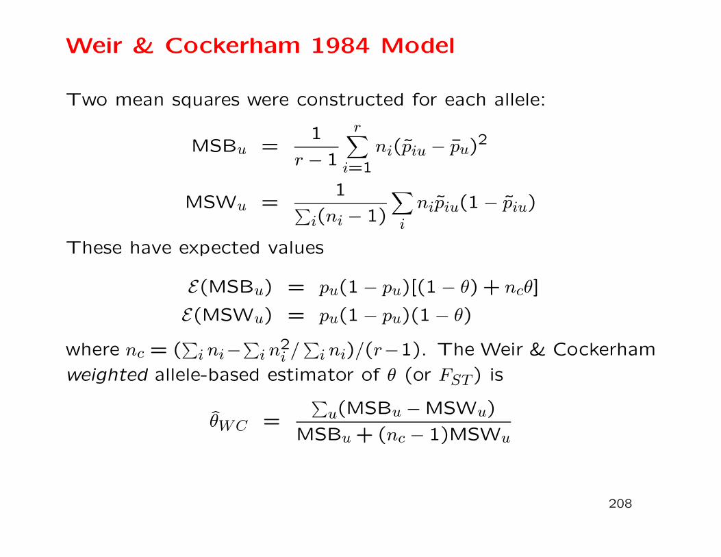
Weir & Cockerham 1984 Model
Two mean squares were constructed for each allele:
MSBu =1
r − 1
r∑
i=1
ni(piu − pu)2
MSWu =1
∑
i(ni − 1)
∑
i
nipiu(1 − piu)
These have expected values
E(MSBu) = pu(1 − pu)[(1 − θ) + ncθ]
E(MSWu) = pu(1 − pu)(1 − θ)
where nc = (∑
i ni−∑
i n2i /∑
i ni)/(r−1). The Weir & Cockerham
weighted allele-based estimator of θ (or FST) is
θWC =
∑
u(MSBu −MSWu)
MSBu + (nc − 1)MSWu
208

Weir & Cockerham 1984 Estimator
Under the β approach described here, the Weir and Cockerham
estimator has expectation
E(θWC) =θWc − θBc +Q
1 − θBc +Qinstead of
θW − θB
1 − θB
where
θWc =
∑
i nciθi
∑
i nci
, θBc =
∑
i 6=i′ nini′θii′
∑
i 6=i′ nini′
nci = ni −n2i
∑
i ni, nc =
1
r − 1
∑
i
nci
Q =1
(r − 1)nc
∑
i
(
nin
− 1
)
θi
If the Weir and Cockerham model holds (θi = θ), or if ni = n, or
if nc is large, then Q = 0.
209

WC84 vs Beta Allele-based Estimators
0.00 0.05 0.10 0.15 0.20 0.25
0.0
00.0
50.1
00.1
50.2
00.2
5
HapMap Fst estimates: no SNP filtering
Bhatia et al
Weir &
Cockerh
am
FWT estimates for HapMap III, using all 87,592 SNPs on chromosome 1.
(Bhatia et al, 2013, Genome Research 23:1514-1521.)
210

WC vs Unweighted Estimator
0.00 0.05 0.10 0.15 0.20 0.25
0.0
00.0
50.1
00.1
50.2
00.2
5
HapMap Fst estimates: SNP filtering
Bhatia et al
Weir &
Cockerh
am
FWT estimates for HapMap III, using the 42,463 SNPs on chromosome 1
that have at least five copies of the minor allele in samples from all 11
populations.
(Bhatia et al, 2013, Genome Research 23:1514-1521.)
211

MLE for Individual Inbreeding Coefficients
To avoid having to choose among moment estimators, we can set
up an MLE although there is more numerical work needed. An
iterative method makes use of Bayes’ theorem. If F represents
the probability the individual in question has two IBD alleles at
a locus, i.e. is inbred at that locus,
Pr(AlAl|inbred) = pl , Pr(AlAl|Not inbred) = p2lPr(Alal|inbred) = 0 , Pr(Alal|Not inbred) = 2pl(1 − pl)
Pr(alal|inbred) = 1 − pl , Pr(alal|Not inbred) = (1 − pl)2
From Bayes’ theorem then
Pr(inbred|AlAl) =Pr(AlAl|inbred)Pr(inbred)
Pr(AlAl)=
plF
p2l + Fpl(1 − pl)
Pr(inbred|Alal) =Pr(Alal|inbred)Pr(inbred)
Pr(Alal)= 0
Pr(inbred|alal) =Pr(alal|inbred)Pr(inbred)
Pr(alal)=
(1 − pl)F
(1 − pl)2 + Fpl(1 − pl)
212

MLE for Individual Inbreeding Coefficients
This suggests an iterative scheme: assign an initial value to
F , and then average the updated values over loci. If Gl is the
genotype at locus l, the updated value F ′ is
F ′ =1
L
L∑
l=1
Pr(inbred|Gl)
This value is then substituted into the right hand side and the
process continues until convergence.
213

Toy Example
Suppose 5 loci have genotypes
MM,Mm,mm,Mm,MM
.
Then the updated estimate is
F ′ =1
5
(
F
p1 + F (1 − p1)+ 0 +
F
(1 − p3) + Fp3+ 0 +
F
p5 + (1 − p5)F
)
If all the pl = 0.5,
F ′ =1
5
(
2F
1 + F+ 0 +
2F
1 + F+ 0 +
2F
1 + F
)
=6F
5(1 + F )
and this converges to F = 0.2.
214

k-coefficients
The coancestry coefficient is the probability of a pair of alleles
being ibd.
For joint genotypic frequencies, and for a more detailed charac-
terization of relatedness of two non-inbred individuals, we need
the probabilities that they carry 0, 1, or 2 pairs of ibd alleles.
For example: their two maternal alleles may be ibd or not ibd,
and their two paternal alleles may be ibd or not.
The probabilities of two individuals having 0, 1 or 2 pairs of ibd
alleles are written as k0, k1, k2 and θ = 12k2 + 1
4k1.
215
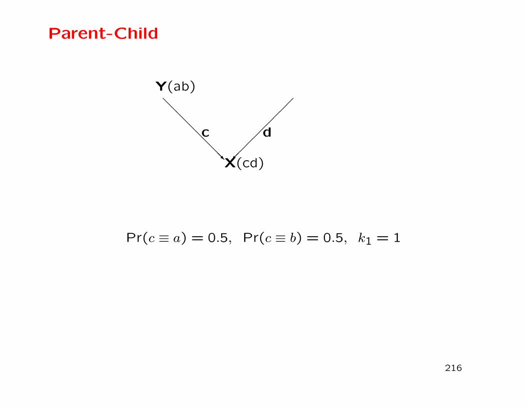
Parent-Child
Y(ab)
X(cd)
@@
@@
@@
@@
@@R
��
��
��
��
��
c d
Pr(c ≡ a) = 0.5, Pr(c ≡ b) = 0.5, k1 = 1
216
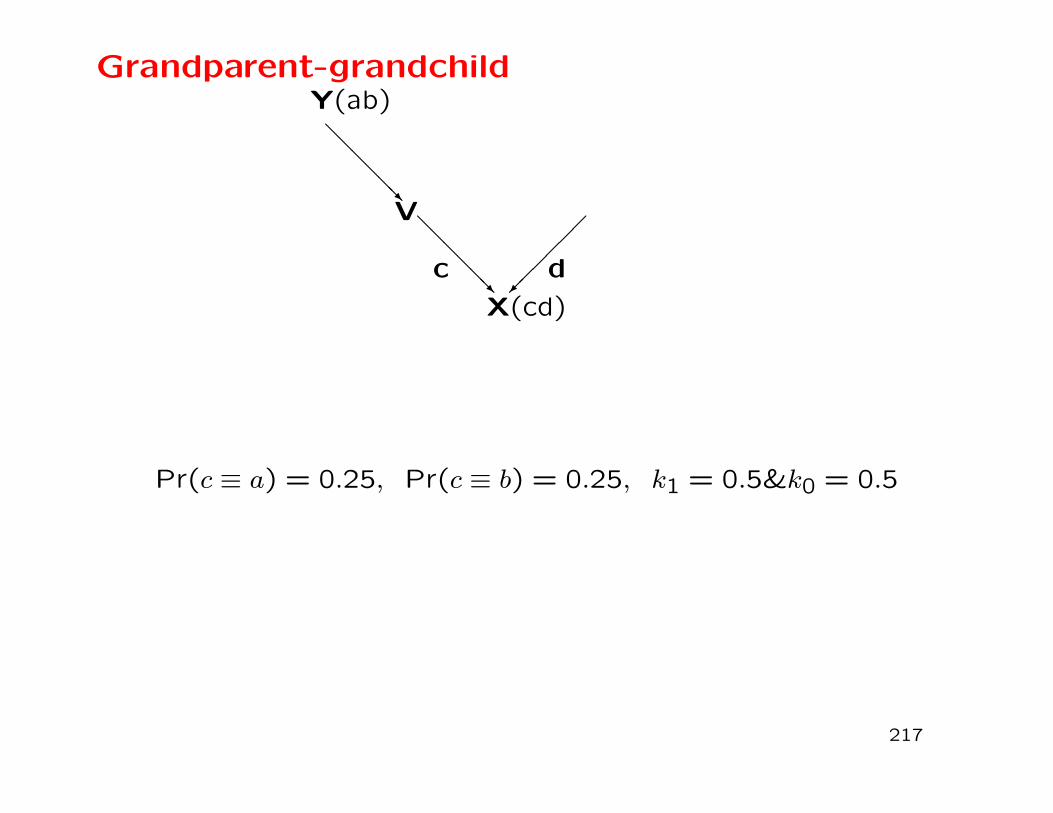
Grandparent-grandchildY(ab)
V
X(cd)
@@
@@
@@R
@@
@@
@@R
��
��
��
c d
Pr(c ≡ a) = 0.25, Pr(c ≡ b) = 0.25, k1 = 0.5&k0 = 0.5
217

Half sibs
U V(ef) W
X Y
a b c d@
@@
@@
@R
��
��
��
@@
@@
@@R
��
��
��
0.5 0.5c ≡ e c ≡ f
0.5 b ≡ e 0.25 0.250.5 b ≡ f 0.25 0.25
Therefore k1 = 0.5 so k0 = 0.5.
218

Full sibsU(ef) V(gh)
X Y?
@@
@@
@@
@@
@@
@@
@@@R ?
��
��
��
��
��
��
���
a b c d
0.5 0.5b ≡ d b 6 ≡d
0.5 a ≡ c 0.25 0.250.5 a 6 ≡c 0.25 0.25
k0 = 0.25, k1 = 0.50, k2 = 0.25
219

First cousins
G H
? ?
HHHHHHHHHHHHj
�������������G C D H@
@@
@@
@R
��
��
��
@@
@@
@@R
��
��
��
a b c dX Y
220
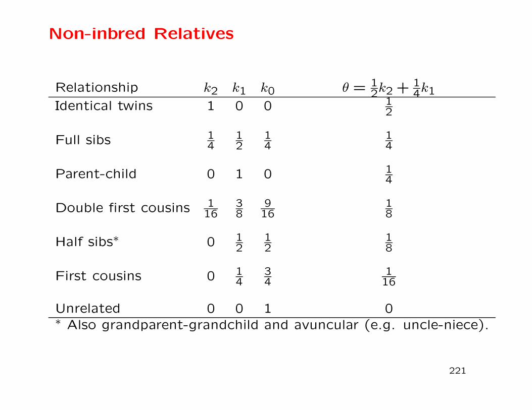
Non-inbred Relatives
Relationship k2 k1 k0 θ = 12k2 + 1
4k1Identical twins 1 0 0 1
2
Full sibs 14
12
14
14
Parent-child 0 1 0 14
Double first cousins 116
38
916
18
Half sibs∗ 0 12
12
18
First cousins 0 14
34
116
Unrelated 0 0 1 0∗ Also grandparent-grandchild and avuncular (e.g. uncle-niece).
221
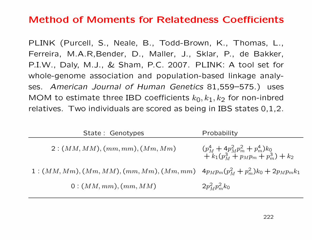
Method of Moments for Relatedness Coefficients
PLINK (Purcell, S., Neale, B., Todd-Brown, K., Thomas, L.,
Ferreira, M.A.R,Bender, D., Maller, J., Sklar, P., de Bakker,
P.I.W., Daly, M.J., & Sham, P.C. 2007. PLINK: A tool set for
whole-genome association and population-based linkage analy-
ses. American Journal of Human Genetics 81,559–575.) uses
MOM to estimate three IBD coefficients k0, k1, k2 for non-inbred
relatives. Two individuals are scored as being in IBS states 0,1,2.
State : Genotypes Probability
2 : (MM,MM), (mm,mm), (Mm,Mm) (p4M + 4p2Mp2m + p4m)k0
+ k1(p3M + pMpm + p3m) + k2
1 : (MM,Mm), (Mm,MM), (mm,Mm), (Mm,mm) 4pMpm(p2M + p2m)k0 + 2pMpmk1
0 : (MM,mm), (mm,MM) 2p2Mp2mk0
222

MOM Approach: k0
Count the number of loci in IBS state i; i = 0,1,2. These num-
bers are N0, N1, N2. The previous table gives the probabilities of
IBS state i given IBD state j. From
Pr(IBS = 0) = Pr(IBS = 0|IBD = 0)Pr(IBD = 0)
sum over loci l to get
N0 =∑
l
2p2l (1 − pl)2 Pr(IBD = 0)
This gives a moment estimate
Pr(IBD = 0) =N0
∑
l 2p2l (1 − pl)
2
223

MOM Approach: k1
From
Pr(IBS = 1) = Pr(IBS = 1|IBD = 0)Pr(IBD = 0)
+ Pr(IBS = 1|IBD = 1)Pr(IBD = 1)
sum over loci to get
N1 = Pr(IBD = 0)∑
l
4pl(1 − pl)[p2l + (1 − pl)
2]
+ Pr(IBD = 1)∑
l
2pl(1 − pl)
but we already have an estimate of Pr(IBD = 0). Therefore
Pr(IBD = 1) =N1 −∑
l 4pl(1 − pl)[p2l + (1 − pl)
2] Pr(IBD = 0)∑
l 2pl(1 − pl)
224

MOM Approach: k2
Having estimated k0 and k1, find k2 as 1 − k0 − k1.
Could then estimate θ as k2/2 + k1/4 or could go to a direct
estimate.
225

PLINK Example
226

MLE for Relatedness Coefficients
For any SNP there are six distinct pairs of genotypes with prob-abilities depending on allele frequencies for that SNP and on aset of three k parameters that are assumed to be the same for allSNPs. If G is the observed pair of genotypes, we know the condi-tional probabilities Pr(G|Di) where the Di represent the identitystates (with probabilities ki).
G Pr(G) =∑
iPr(G|Di)kiMM,MM k2p2M + k1p3M + k0p4M
mm,mm k2p2m + k1p3m + k0p4m
MM,mm 2k0p2Mp2m
MM,Mm 2k1p2Mpm + 4k0p3Mpm
mm,Mm 2k1pMp2m + 4k0pMp3m
Mm,Mm 2k2pMpm + k1pMpm + 4k0p2Mp2m
227

MLE for Relatedness Coefficients
An iterative algorithm for estimating the k’s from observed geno-
types Gl at SNP l is based on Bayes’ theorem for the probability
of descent state Di, i = 0,1,2:
Pr(Di|Gl) =Pr(Gl|Di)Pr (Di)
Pr(Gl)
The procedure begins with initial estimates of the ki = Pr(Di)’s.
The updated estimates are obtained by averaging over L loci:
k′i =1
L
L∑
l=1
(
Pr(Gl|Di)ki∑
j Pr(Gl|Dj)kj
)
, i = 0,1,2
These updated values are then substituted into the right hand
side until they no longer change (or change by less than some
specified small amount).
228

Toy Example
Suppose the 5-locus genotypes for U, V are:
MM,Mm,mm,Mm,MM
and
MM,mm,Mm,Mm,Mm
The updating equations are:
k′2 =1
5
(
p21k2
p21k2 + p32k1 + p41k0+ 0 + 0
+2p4(1 − p4)k2
2p4(1 − p4)k2 + p4(1 − p4)k1 + 4p24(1 − p4)2k0+ 0
)
229

Toy Example
k′1 =1
5
(
p31k1
p21k2 + p32k1 + p41k0+
2p2(1 − p2)2k1
2p2(1 − p2)2k1 + 4p2(1 − p2)3k0
+2p3(1 − p3)
2k12p3(1 − p3)2k1 + 4p3(1 − p3)3k0
+p4(1 − p4)k1
2p4(1 − p4)k2 + p4(1 − p4)k1 + 4p24(1 − p4)2k0
+2p25(1 − p5)k1
2p25(1 − p5)k1 + 4p35(1 − p5)k0
)
230
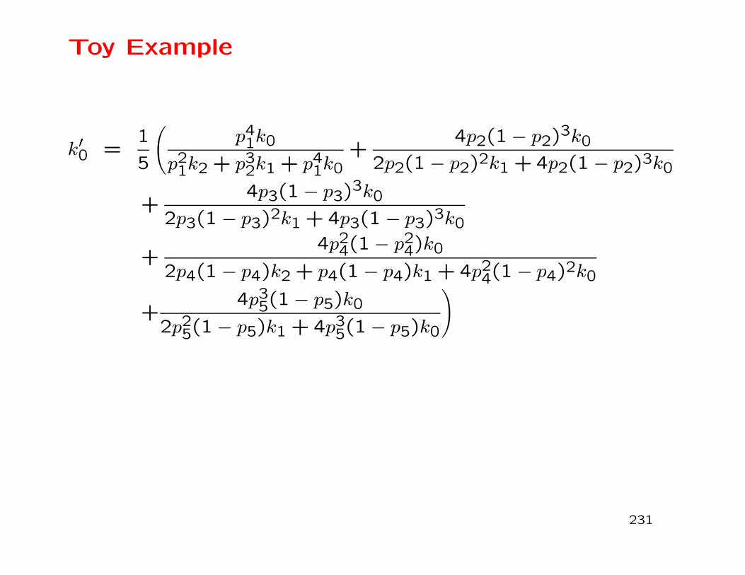
Toy Example
k′0 =1
5
(
p41k0
p21k2 + p32k1 + p41k0+
4p2(1 − p2)3k0
2p2(1 − p2)2k1 + 4p2(1 − p2)3k0
+4p3(1 − p3)
3k02p3(1 − p3)2k1 + 4p3(1 − p3)3k0
+4p24(1 − p24)k0
2p4(1 − p4)k2 + p4(1 − p4)k1 + 4p24(1 − p4)2k0
+4p35(1 − p5)k0
2p25(1 − p5)k1 + 4p35(1 − p5)k0
)
231

“RELPAIR” calculations
This approach compares the probabilities of two genotypes un-
der alternative hypotheses; H0: the individuals have a specified
relationship, versus H1: the individuals are unrelated. The alter-
native is that k0 = 1, k1 = k2 = 0 so the likelihood ratios for the
two hypotheses are:
LR(MM,MM) = k0 + k1/pM + k2/p2M
LR(mm,mm) = k0 + k1/pm + k2/p2m
LR(Mm,Mm) = k0 + k1/(4pMpm) + k2/(2pMpm)
LR(MM,Mm) = k0 + k1/(2pM)
LR(mm,Mm) = k0 + k1/(2pm)
LR(MM,mm) = k0
232

Testing relationship
Hypotheses about alternative pairs of relationships may be tested
with likelihood ratio test statistics. These ratios are the prob-
ability of the observed pair of genotypes under one hypothesis
divided by the probability under the alternative hypothesis. These
ratios are multiplied over (independent) loci.
Each hypothesis is described by a set of k’s and there are three
hypotheses likely to be of interest:
1. individuals are unrelated (k0 = 1)
2. individuals have a specified (or annotated) relationship (k’s
specified)
or 3. individuals are related to an extent measured by the esti-
mated k’s.
233