summer school in applied psychometric principles
TRANSCRIPT

Summer School in Applied Psychometric Principles
Peterhouse College
13th to 17th September 2010

The Rasch Model
Day 3
Jan R. Böhnke
University of Trier, Germany
2

Topics already covered
• We have…– Introduced IRT
– Introduced simple models for binary responses
– Discussed IRT assumptions
– Introduced models for polytomous responses
– Discussed assessment of fit for these models

Today
• We will spend a day with the Rasch Model
• Why that?– Rasch Model is a very simple test model
– which has extraordinary measurement qualities
– can be generalized to several applications
– and which is testable

The Rasch Model
• The Rasch model can be seen as a very reduced / restricted version of the models we already encountered in the course:– the slopes for all items are constrained to be equal (usually Dα = 1)
– no guessing parameter (c = 0)
5
( ) ( )( )
( )1 | 11
i i
i i
Da b
i i i Da b
eP u c ce
−
−= = + −+
θ
θθ
)(
)(
1)|1(
i
i
b
b
i eeuP −
−
+== θ
θ
θ

The Rasch Model
-4 -2 0 2 4
0.0
0.2
0.4
0.6
0.8
1.0
ICCs for Mobility survey items
Latent Dimension
Pro
babi
lity
to S
olve
Item 1Item 2Item 3Item 4Item 5Item 6Item 7Item 8

The Rasch Model
• The fact that only one parameter is modeledleads to the models‘ most importantconsequence:– the ICCs are non-intersecting
– thereby holds for any comparison of persons oritems:
wvwivi xPxP θθ >⇔=>= )0()1(

The Rasch Model
wvwivi xPxP θθ >⇔=>= )0()1(-4 -2 0 2 4
0.0
0.2
0.4
0.6
0.8
1.0
ICCs for Mobility survey items
Latent Dimension
Pro
babi
lity
to S
olve
Item 1Item 2Item 3Item 4Item 5Item 6Item 7Item 8

• This feature of the Rasch Model is called„specific objectivity“; when the Rasch model holds:– irrespective of which combination of items from a
scale, the same ordering of persons is obtained
– irrespective of what subsample of persons, theitems are ordered the same way according to theirdifficulty
The Rasch Model
wvwivi xPxP θθ >⇔=>= )0()1(

• because both these orderings are stable(within measurement error):– it is not important which combination of items
was solved by a respondent;
– and from that follows that the sum of solved itemscontains all information about the respondent‘sposition on the latent trait
The Rasch Model
wvwivi xPxP θθ >⇔=>= )0()1(

• this principle of „specific objectivity“ providesthe possibility to construct two specific teststhat test whether the data is Rasch-scalable ornot:– the Andersen Likelihood Ratio Test: checks
whether the invariance of item parameters in different subpopulation holds
– the Martin Löf Test: checks whether the personparameters are invariant by splitting the scale intodifferent subsets of items
The Rasch Model

Sideline: Guttman Scaling
• In Guttman scaling onlyspecific patterns allowed:– items ordered according to
their difficulty
– a person solving a moredifficult item has to solve all items that are easier thanthat 1111
0111001100010000
Items

wvwivi xx θθ >⇔=∧= )0()1(
• „deterministic model“
• only ordinal measurementpossible but score also represents all availableinformation on respondents
• Measurement Theorem: 11110111001100010000
Items
Sideline: Guttman Scaling
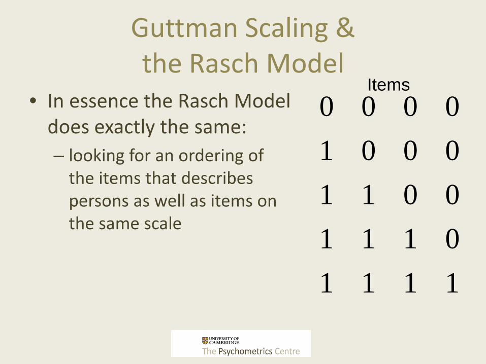
• In essence the Rasch Model does exactly the same:– looking for an ordering of
the items that describespersons as well as items on the same scale
11110111001100010000
Items
Guttman Scaling &the Rasch Model

• the Rasch model is in a sense completely different:– it acknowledges
measurement error: Guttman structure would bethe ideal pattern, but deviations from that arepossible
– „probabilistic model“ 11110111001100010000
Items
Guttman Scaling &the Rasch Model

• the Rasch model is in a sense completely different:– by introducing a well-
behaved mathematicalfunction to describe therelationship between thetrait and the probability, it ispossible to scale the itemsand scores on a (more than) interval continuum
11110111001100010000
Items
Guttman Scaling &the Rasch Model

• based on the data itcan be assessed, where on the latent continuum the item is solved with a probability of 50%
• since the slope isdefined by themathematicalfunction, distancesbetween thelocations can bemeasured
-4 -2 0 2 4
0.0
0.2
0.4
0.6
0.8
1.0
ICCs for Mobility survey items
Latent Dimension
Pro
ba
bili
ty to
So
lve
Item 1Item 2Item 3Item 4Item 5Item 6Item 7Item 8
Guttman Scaling &the Rasch Model

Dimensionality or Local independence assumption
• Item responses are independent after controlling for (conditional on) the latent trait
• There is only one dimension explaining variance in the item responses– based on this assumption non-parametric tests
can already be employed to check whether the data fits the model BEFORE we even estimate the model (e.g. Ponocny, I. (2001). Psychometrika, 66, 437-460.)
18

Features of the Rasch-Model
• Two core differences to other IRT models: – it can be tested whether the respondents‘
patterns in the answer vectors comply with theassumtion of the Rasch Model (tests not based on „by-proxy“ tests with factor analysis)
– Compared to the other models the score is the„sufficient statistic“; in the other models it is a weighted sum

Estimating item parameters
• Joint maximum likelihood estimation (JML)– Uses observed frequencies of response patterns– Starting values for ability as proportion correct
1. Estimate item parameters2. Use item parameters to re-estimate ability
– Repeat last two steps until estimates do not change• Marginal maximum likelihood (MML)
– Uses expected frequencies of each response pattern– EM (Estimation and Maximisation) by Bock & Aitken ( 1981) is
popular• Conditional maximum likelihood (CML)
– Uses sufficient statistics to exclude trait level parameters (only applies to the Rasch models)

Estimating item parameters
• Conditional maximum likelihood (CML)
(Wilhem Kempf, University of Konstanz)
Formulas not important in detail, but:the estimator for everyitem parameter dependsa) on the interaction of
the location of all otheritems
b) conditional on all testscores

Finding the examinee parameter• Maximum likelihood (ML)
– Maximising the likelihood function (iterative process)– ML estimator is unbiased, and its errors are normally distributed– Problems with ML is that convergence is not guaranteed with aberrant
responses, and no estimator exists for all correct/incorrect responses
• Warm’s Maximum Likelihood (WML)– often employed (e.g. WINMIRA) because it provides estimates for full/empty
response patterns– more computational intensive than ML– more central estimates; SEs equal to ML
• Spline interpolation– estimator based on the relationship between scores and estimated person
parameters– employed in eRm


Practical: Mobility survey
• The dimension of interest is women’s mobility of social freedom.
• Women were asked whether they could engage in the following activities alone (1 = yes, 0 = no):
25

Estimation in R – eRm
library(eRm)
ResMob<-RM(Itemmatrix,se=TRUE,sum0=TRUE)
Itemmatrix is the Matrix containing theresponses
se=TRUE (standard errors are estimated)
sum0=TRUE (b‘s are normed on 0)

Plotting
plotjointICC(ResMob, main="ICCs for dichotomous Mobility items", xlim=c(-5,5),legpos="topleft")
plotjointICC(ResMob, main="ICCs for dichotomous Mobility items", item.subset=c(1,5,7))

-4 -2 0 2 4
0.0
0.2
0.4
0.6
0.8
1.0
ICCs for dichotomous Mobility items
Latent Dimension
Pro
babi
lity
to S
olve
Item 1Item 2Item 3Item 4Item 5Item 6Item 7Item 8
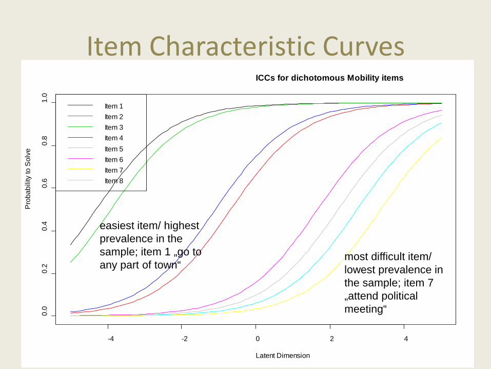
Item Characteristic Curves
easiest item/ highestprevalence in thesample; item 1 „go toany part of town“
most difficult item/ lowest prevalence in the sample; item 7 „attend politicalmeeting“

Plotting
plotICC(ResMob,empICC=list("kernel"),empCI=list(),main="ICCs for dichotomous Mobility items")

Plotting
-4 -2 0 2 4
0.0
0.4
0.8
ICCs for dichotom
Latent Dimension
Pro
babi
lity
to S
olve
-4 -2 0 2 4
0.0
0.2
0.4
0.6
0.8
1.0
ICCs for dichotomous Mobility items
Latent Dimension
Pro
babi
lity
to S
olve
Item 1Item 2Item 3Item 4Item 5Item 6Item 7Item 8
Item Characteristic Curves
easiest item/ highestprevalence in thesample; item 1 „go toany part of town“
most difficult item/ lowest prevalence in the sample; item 7 „attend politicalmeeting“

Joint distribution of items and personparameters
Item 7
Item 5
Item 8
Item 6
Item 2
Item 4
Item 3
Item 1
-4 -3 -2 -1 0 1 2 3 4Latent Dimension

Estimating the person parameters
PersMob<-person.parameter(ResMob)
plot(PersMob)

Relationship between scores andperson parameters
• every score can betransformed into thescale-free metric of theperson parameters
• not related in linear fashion (esp. in thetails)
• also: there are only asmany personparameters estimatedas possible scores(unlike in the other IRT models) 0 2 4 6 8
-6-4
-20
24
Plot of the Person Parameters
Person Raw Scores
Per
son
Par
amet
ers
(The
ta)

What if…?
• What would be won if the Rasch-Model fitted the data?– we know that the summed item score can be used as a simple
descriptive measure for the ability (was also used to estimate the model)
– we also would have the person parameters to represent the ability on a (better than) equal interval level
– we would know that the test is fair at any rate („specific objectivity“)
• The nice thing about the Rasch-Model is, that clear predictions about the nature of the data follow from the model formulation and these predictions can be easily tested

Testing the Rasch Model
• Non-Parametric tests:– Ponocny, I. (2001). Psychometrika, 66, 437-460.
– before estimating the Rasch Model at all we could test whether the observed item responses of the persons would be expected if the test was Raschscaled
– not covered in detail here

Testing the Rasch Model
• Parametric Tests based on “specific objectivity”:
– ANDERSEN‘S LR-TEST: all estimated parameters are independent of the subgroup of the sample in which they are estimated (e.g. gender)
– MARTIN LÖF-TEST: irrespective of which items are used, the comparison between two test persons should result in the same ordering

Andersen‘s Likelihood Ratio Test
• Procedure:– The Rasch Model is estimated independently in both/all
subgroups– and then the fit is compared using the likelihood:
• with df=(g-1)*(k-1); with g = number of subgroups andk = number of items
• these Likelihoods should be the same, if theitemparameters (δi) were the same in all subgroups g,i.e. the test should be non-significant
38
))ouphood(Subgr(LN(Likeliset) data hood(full(LN(Likeli*-2І g∑+=g
χ

Andersen‘s Likelihood Ratio Test
• the default test is with high vs. low scorergroups
• Sample is divided into two groups:– a: scores <= median;
– b: scores > median
• Andersen1<-LRtest(ResMob,se=TRUE)
• summary(Andersen1)
39

Andersen‘s Likelihood Ratio Test
• the default test is with high vs. low scorergroups
• Sample is divided into two groups:– a: scores <= median;– b: scores > median
• χ² = 78.36 with df=7; p < .001• the 8 items do not have the same difficulty
parameters in both samples
40

Andersen‘s Likelihood Ratio Test
41
• Plotting:
plotGOF(Andersen1,main="Graphical model check, Median",tlab="number", ctrline=list(gamma=0.95, col="blue", lty="dashed"), conf=list(),xlim=c(-5,5),ylim=c(-5,5))

-4 -2 0 2 4
-4-2
02
4
Graphical model check, Media
Beta for Group: Raw Scores <= Median
Bet
a fo
r Gro
up: R
aw S
core
s >
Med
ian
1
2
3
4
5
6
7
8

Andersen‘s Likelihood Ratio Test
• no covariates in the data file; therefore simulate one:
Mobility$covariate<-with(Mobility,rbinom(8445,1,.5))
Andersen2<-LRtest(ResMob,se=TRUE,splitcr=(Mobility$covariate))
43

Andersen‘s Likelihood Ratio Test
• the random split results in a non-significanttest statistic:
• χ² = 3.15 with df=7; p = .87
• the 8 items do have the same difficultyparameters in both samples
44

Andersen‘s Likelihood Ratio Test
45
-4 -2 0 2 4
-4-2
02
4
Graphical model check, covar
Beta for Group: (Mobility$covariate) 0
Bet
a fo
r Gro
up: (
Mob
ility
$cov
aria
te) 1
1
2
3
4
5
6
7
8

Wald Test
• Both tests provide only information on the fact that thedifference between groups is at least for one item parameter big enough, to produce a significant test statistic
• Wald-Tests can be used to test the differences between thesubgroups for every item
46
22
21
21€€
ii
iiiz
σσ
ββ
+
−=

Wald Test
• Syntax for split with median raw score splitting:
• Wald1<-Waldtest(ResMob)
47

Wald Test
• In this example done for median of ability
• The following items fail this test:– Item 3: p = .002
– Item 8: < .001
• typical post-hoc questions apply: Type I error, cross-validation,…
48

Differential Item Functioning
• These ideas are closely connected to thequestion of Differential Item Functioning (DIF)
• DIF explores whether there are systematic differences between groups in the difficulty of endorsing specific item categories
• these should not be present (or corrected for), because they question the fairness of a specific test
• topic of tomorrow
49

• Procedure:
– The Rasch Model is estimated independently in bothITEM subgroups
– then the fit is compared using the likelihood:
– For two subgroups with df=(l1*l2-1); with l1 = number of items in subgroup 1 and l2 = number of items in subgroup 2
– these Likelihoods should be the same, if the itemparameters (θj) were the same in all subgroups, i.e. the test should be non-significant
50
))ouphood(Subgr(LN(Likeliset) data hood(full(LN(Likeli*-2І l∑+=l
χ
Martin Löf Test

• the default test is with items high vs. Low in difficulty
• Sample is devided into two groups:– a: itemparameter <= median (Items: 1, 2, 3, 4);
– b: itemparameter > median (Items: 5, 6, 7, 8);
• χ² = ~3438 with df=15; p <<< .001• The items are (at least with this split criterion) not homogeneous
51
Martin Löf Test

• Other splits possible, e.g.:
– One has a hypothesis which items should be groupedtogether more closely
– Random splits
• Please think of sub grouping / sub scaling! Then we will perform the test for this specific comparison!
52
Martin Löf Test

Assessing Model Fit: Summary
• (Some) Ways to test the fit of the Rasch-Model:– Andersen‘s LR-Test: Itemparameters the same for
different subgroups?
– Wald-Tests: Itemparameters the same for different subgroups (pay attention to alpha-level!)
– Martin-Löf-Test: Personparameters are the same when resulting from different item-sets
53

Assessing Model Fit: Summary
• Splits in this regard are usually only as good asthe observed criteria
• Rost & von Davier (1997) proposed therefore:– estimate the Rasch-Model on your data
– estimate a two class Mixed Rasch Model on thesame data to identify the maximal possibledifferences between persons in response patterns
– LR-test between these models or (my opinion) Andersen test with these groups
54


Polytomous Rasch Models
• The question for polytomous IRT models is, how the different categories can be mappedon the latent continuum
• already seen: Graded Response Model
• In the Rasch perspective especially the Partial Credit Model is of interest
• and the constraint version of the so-calledRating Scale Model

Generalized Partial Credit Model• The model is:
• Easier to see step by step (assume 3 categories):– Probability of completing 0 steps
– Probability of completing 1 step
57
( ) [ ][ ] ( ) ( ) ( )0
1 1 2
exp 0exp 0 exp 0 exp 0i
i i i i i i
Pa b a b a b
θθ θ θ
=+ + − + + − + −
( ) ( )[ ] ( ) ( ) ( )
10
1 1 2
exp 0exp 0 exp exp 0
i ii
i i i i i i
a bP
a b a b a bθ
θθ θ θ
+ − =+ − + + − + −
( )( )
( )0
0 0
exp
exp
x
i iss
ix m r
i isr s
a bP
a b
θθ
θ
=
= =
−=
−
∑
∑ ∑

The Partial Credit logic• Created specifically to handle items that require logical
steps, and partial credit can be assigned for completing some steps (common in mathematical problems)
• Completing a step assumes completing below• Computing probability of response to each category is
direct (“divide-by-total”):– Probability of responding in category x (completing x
steps) is associated with ratio of• odds of completing all steps before and including this one, and• odds of completing all steps
– Each step’s odds are modelled like in binary logistic models• For an item with m+1 response categories, m step difficulty
parameters b1…bm are modelled
58

Interpretation
• Step difficulty parameters have an easy graphical interpretation – they are points where the category lines cross
• Relative step difficulty reflects how easy it is to make transition from one step to another – Step difficulties do not have
to be ordered– “Reversal” happens if a
category has lower probability than any other at all levels of the latent trait
-4 -2 0 2 4
0.0
0.2
0.4
0.6
0.8
1.0
ICC plot for item aBDI1001
Latent Dimension
Pro
babi
lity
to S
olve
Category 0Category 1Category 2Category 3

Estimating a Rating Scale Model in eRm
• starting with the restricted case of the RSM:
• The function “RSM” is used:
Result<-RSM(data, se=TRUE, sum0=TRUE)

Rating Scale Model
• circles: thresholds
• black dots: difficulty(comparableto item mean)
aBDI1009aBDI1018aBDI1012aBDI1020aBDI1007aBDI1014aBDI1003aBDI1005aBDI1006aBDI1021aBDI1010aBDI1002aBDI1001aBDI1017aBDI1011aBDI1008aBDI1015aBDI1004aBDI1016aBDI1013
-3 -2 -1 0 1 2 3Latent Dimension
1 2 31 2 3
1 2 31 2 3
1 2 31 2 31 2 3
1 2 31 2 3
1 2 31 2 31 2 3
1 2 31 2 31 2 31 2 31 2 3
1 2 31 2 3
1 2 3
Person-Item Map
PersonParameterDistribution

Rating Scale Model
• the RSM imposes the exact same differencesbetween category steps on every item
• in eRm estimated via– estimation of the first threshold
– and estimation of difference parameters between first and second as well as first and third threshold

Rating Scale Model
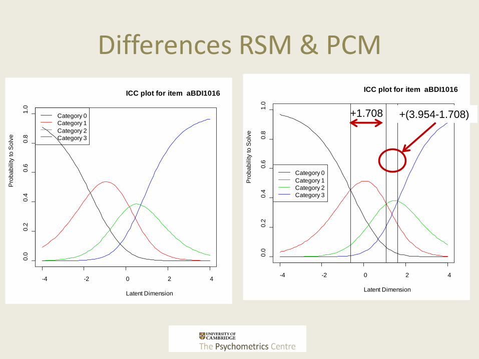
• Category parameter 0/1: first threshold, estimated
• Category parameter 1/2: second threshold, 1.708
• Category parameter 2/3: third threshold, 3.954

Rating Scale Model
• Categoryparameter 0/1: first threshold, estimated; Item 16 (sleepdisturbances): -.622
-4 -2 0 2 4
0.0
0.2
0.4
0.6
0.8
1.0
ICC plot for item aBDI1016
Latent Dimension
Pro
babi
lity
to S
olve
Category 0Category 1Category 2Category 3
+1.708 +(3.954-1.708)

-4 -2 0 2 4
0.0
0.2
0.4
0.6
0.8
1.0
ICC plot for item aBDI1006
Latent Dimension
Pro
babi
lity
to S
olve
Category 0Category 1Category 2Category 3
Rating Scale Model
• Categoryparameter 0/1: first threshold, estimated; Item 06 (feeling / waiting to bepunished): .018
+1.708 +(3.954-1.708)

Differences RSM & PCM
• the major difference between these twomodels is– the PCM allows every item to have its own
structure of category steps
– whereas the RSM imposes the exact same differences between category steps on every item
– (also models possible that use the same ratios etc)
– AND every item can have its own number ofcategories

• the Partial Credit Model makes it possible that every item has its own pattern of thresholds
• in eRm estimated via– estimation of all thresholds of the items but one
– (either parameterized that that have to sum to 0 or the first threshold is set to be 0)
Differences RSM & PCM

• Category parameter 0/1: first threshold, estimated
• Category parameter 1/2: second threshold, estimated
• Category parameter 2/3: third threshold, estimated
Differences RSM & PCM
Differences RSM & PCM
-4 -2 0 2 4
0.0
0.2
0.4
0.6
0.8
1.0
ICC plot for item aBDI1016
Latent Dimension
Pro
babi
lity
to S
olve
Category 0Category 1Category 2Category 3
+1.708 +(3.954-1.708)
-4 -2 0 2 4
0.0
0.2
0.4
0.6
0.8
1.0
ICC plot for item aBDI1016
Latent Dimension
Pro
babi
lity
to S
olve
Category 0Category 1Category 2Category 3

-4 -2 0 2 4
0.0
0.2
0.4
0.6
0.8
1.0
ICC plot for item aBDI1006
Latent Dimension
Pro
babi
lity
to S
olve
Category 0Category 1Category 2Category 3
Differences RSM & PCM
+1.708+(3.954-1.708)
-4 -2 0 2 4
0.0
0.2
0.4
0.6
0.8
1.0
ICC plot for item aBDI1006
Latent Dimension
Pro
babi
lity
to S
olve
Category 0Category 1Category 2Category 3

Differences RSM & PCM
aBDI1009aBDI1018aBDI1012aBDI1020aBDI1007aBDI1014aBDI1003aBDI1005aBDI1006aBDI1021aBDI1010aBDI1002aBDI1001aBDI1017aBDI1011aBDI1008aBDI1015aBDI1004aBDI1016aBDI1013
-3 -2 -1 0 1 2 3Latent Dimension
1 2 31 2 3
1 2 31 2 3
1 2 31 2 31 2 3
1 2 31 2 3
1 2 31 2 31 2 3
1 2 31 2 31 2 31 2 31 2 3
1 2 31 2 3
1 2 3
Person-Item Map
PersonParameterDistribution
aBDI1009aBDI1012aBDI1018aBDI1020aBDI1007aBDI1003aBDI1005aBDI1014aBDI1021aBDI1015aBDI1002aBDI1001aBDI1017aBDI1006aBDI1011aBDI1010aBDI1013aBDI1008aBDI1004aBDI1016
-4 -3 -2 -1 0 1 2 3Latent Dimension
1 3 21 2 3
1 2 31 2 3
1 2 31 2 3
1 2 31 2 3
1 2 31 2 3
1 2 31 2 3
1 2 33 1 2
1 2 33 1 21 2 31 3 2
1 2 31 2 3
* * * *
Person-Item Map
PersonParameterDistribution

Differences RSM & PCM
• BDI item 9, suicidal ideation
-4 -2 0 2 4
0.0
0.2
0.4
0.6
0.8
1.0
ICC plot for item aBDI1009
Latent Dimension
Pro
babi
lity
to S
olve
Category 0Category 1Category 2Category 3
-4 -2 0 2 4
0.0
0.2
0.4
0.6
0.8
1.0
ICC plot for item aBDI1009
Latent Dimension
Pro
babi
lity
to S
olve
Category 0Category 1Category 2Category 3

Differences PCM &
-4 -2 0 2 4
0.0
0.2
0.4
0.6
0.8
1.0
ICC plot for item aBDI1016
Latent Dimension
Pro
babi
lity
to S
olve
Category 0Category 1Category 2Category 3
-4 -2 0 2 4
0.0
0.2
0.4
0.6
0.8
1.0
Item Response Category Char
Ability
Pro
babi
lity
1234

-4 -2 0 2 4
0.0
0.2
0.4
0.6
0.8
1.0
ICC plot for item aBDI1006
Latent Dimension
Pro
babi
lity
to S
olve
Category 0Category 1Category 2Category 3
-4 -2 0 2 4
0.0
0.2
0.4
0.6
0.8
1.0
Item Response Category Char
Ability
Pro
babi
lity
1234
Differences PCM &

-4 -2 0 2 4
0.0
0.2
0.4
0.6
0.8
1.0
ICC plot for item aBDI1009
Latent Dimension
Pro
babi
lity
to S
olve
Category 0Category 1Category 2Category 3
Differences PCM &

Testing polytomous Rasch Models
• since in the estimation process for CML polytomous items are treated as if they weredichotomous items
• polytomous Rasch Models are testable in thesame way as dichotomous Rasch Models

Testing polytomous Rasch Models
• Test with RSM
• p < .001
0 2 4 6
02
46
Graphical model check, Media
Beta for Group: Raw Scores <= Median
Bet
a fo
r Gro
up: R
aw S
core
s >
Med
ian
aBDI1001.c3
aBDI1002.c1
aBDI1004.c2
aBDI1005.c3
aBDI1008.c2
aBDI1010.c3
aBDI1014.c2

Testing polytomous Rasch Models
• Test with PCM
• p < .001
-4 -2 0 2 4 6
-4-2
02
46
Graphical model check, Media
Beta for Group: Raw Scores <= Median
Bet
a fo
r Gro
up: R
aw S
core
s >
Med
ian
aBDI1001.c1aBDI1001.c2
aBDI1001.c3
aBDI1004.c2
aBDI1009.c2
aBDI1009.c3
aBDI1013.c3
aBDI1017.c2
aBDI1020.c3

RSM vs PCM
• RSM needs substantially less parameters
• this was before the 2000s a substantial advantage
• today in my opinion no reason to use thismodel anymore
• (despite the case in which LR test betweenRSM and PCM shows no significant difference)

Rasch vs. 2PL or 3PL Model? (or PC vs. GR and GPCM?)
• This comparison has been of interest for many years, and generated quite emotional debate.
• Rasch model has many desirable properties– estimation of parameters is straightforward,– sample size does not need to be big,– number of items correct is the sufficient statistic for
person’s score, – measurement is completely additive,– specific objectivity (more on this tomorrow).
• But your data might not fit the Rasch model…
81

Why Rasch?
• often critique: there are no data, that fit thatmodel
• several responses are possible:– bad theories produce bad empirics
– Rasch is a very simple model and reality is not simple (LLTM, LLRA, Mix-Rasch, Multidimensional-/ Nominal-Rasch model,…)
– BUT it is a model where in detail can be tested, whether it fits the data, or not

Rasch vs. 2PL or 3PL Model? (Cont.)
• Two-parameter logistic model is more complex– Often fits data better than the Rasch model– Requires larger samples (500+)
• Three-parameter logistic model is even more complex– Fits data where guessing is common better– Estimation is complex and estimates are not
guaranteed without constraints– Sample needs to be large in applications.
83

Choice of model must be pragmatic
• Desirable measurement properties of the Rasch model may make it a target model to achieve when constructing measures– Rasch maintained that if items have different discriminations, the
latent trait is not unidimensional
• However, in many applications it is impossible to change the nature of the data– Take school exams with a lot of varied curriculum content to be
squeezed in the test items
• There must be a pragmatic balance between the parsimony of the model and the complexity of the application

Rasch as model of choice
• for many applications also models with moreparameters might be able to reliablydiscriminate between different levels of a continuous latent trait

Rasch as model of choice
• but the Rasch Model it is the only test model that ensures specific objectivity and in whichthe local stochastic independence assumptionis testable
• therefore, especially in high stakes testingsituations the Rasch model proves to beextremely useful