Superdiffusive dispersals impart the geometry of underlying random walks

V. Zaburdaev,1, 2 I. Fouxon,3 S. Denisov,4, 5, 6 and E. Barkai3

1Max Planck Institute for the Physics of Complex Systems,Nothnitzer Strasse 38, D-01187 Dresden, Germany

2Institute of Supercomputing Technologies, Lobachevsky State University of Nizhny Novgorod, 603140 N. Novgorod, Russia3Department of Physics, Institute of Nanotechnology and Advanced Materials, Bar-Ilan University, Ramat-Gan, 52900, Israel

4Department of Applied Mathematics, Lobachevsky State University of Nizhny Novgorod, 603140 N. Novgorod, Russia5Sumy State University, Rimsky-Korsakov Street 2, 40007 Sumy, Ukraine

6Institute of Physics, University of Augsburg, Universitatsstrasse 1, D-86135, Augsburg Germany

It is recognised now that a variety of real-life phenomena ranging from diffuson of cold atomsto motion of humans exhibit dispersal faster than normal diffusion. Levy walks is a model thatexcelled in describing such superdiffusive behaviors albeit in one dimension. Here we show that, incontrast to standard random walks, the microscopic geometry of planar superdiffusive Levy walks isimprinted in the asymptotic distribution of the walkers. The geometry of the underlying walk canbe inferred from trajectories of the walkers by calculating the analogue of the Pearson coefficient.

PACS numbers: 05.40.Fb,02.50.Ey

Introduction. The Levy walk (LW) model [1–3] wasdeveloped to describe spreading phenomena that werenot fitting the paradigm of Brownian diffusion [4]. Stilllooking as a random walk, see Fig. 1, but with a verybroad distribution of excursions’ lengths, the correspond-ing processes exhibit dispersal faster than in the caseof normal diffusion. Conventionally, this difference isquantified with the mean squared displacement (MSD),〈r2(t)〉 ∝ tα, and the regime with α > 1 is called super-diffusion. Examples of such systems range from coldatoms moving in dissipative optical lattices [5] to T cellsmigrating in the brain tissue [6]. Most of the existingtheoretical results, however, were derived for one dimen-sional LW processes [3]. In contrast, real life phenom-ena – biological motility (from bacteria [7] to humans [8]and autonomous robots [9, 10]), animal foraging [11, 12]and search [13] – happen in two dimensions. Somewhatsurprisingly, generalizations of the Levy walks to two di-mensions are still virtually unexplored.

In this work we extend the concept of LWs to twodimensions. Our main finding is that the microscopic ge-ometry of planar Levy walks reveals itself in the shapeof the asymptotic probability density functions (PDF)P (r, t) of finding a particle at position r at time t after itwas launched from the origin. This is in a sharp contrastto the standard 2D random walks, where, by virtue of thecentral limit theorem (CLT) [14], the asymptotic PDFsdo not depend on geometry of the walks and have a uni-versal form of the two-dimensional Gaussian distribution[15, 16].

Models. We begin with a core of the Levy walk concept[1, 2]: A particle performs ballistic moves with constantspeed, alternated by instantaneous re-orientation events,and the length of the moves is a random variable witha power-law distribution. Because of the constant speedv0, the length li and duration τi of the i-th move arelinearly coupled, li = v0τi. As a result, the model can be

equally well defined by the distribution of ballistic move(flight) times

ψ(τ) =1

τ0

γ

(1 + τ/τ0)1+γ, τ0, γ > 0. (1)

Depending on the value of γ, it can lead to a dispersalα = 1, typical for normal diffusion (γ > 2), and very longexcursions leading to the fast dispersal with 1 < α ≤ 2in the case of super-diffusion (0 < γ < 2). At eachmoment of time t the finite speed sets the ballistic frontbeyond which there are no particles. Below we considerthree intuitive models of two-dimensional superdiffusivedispersals.

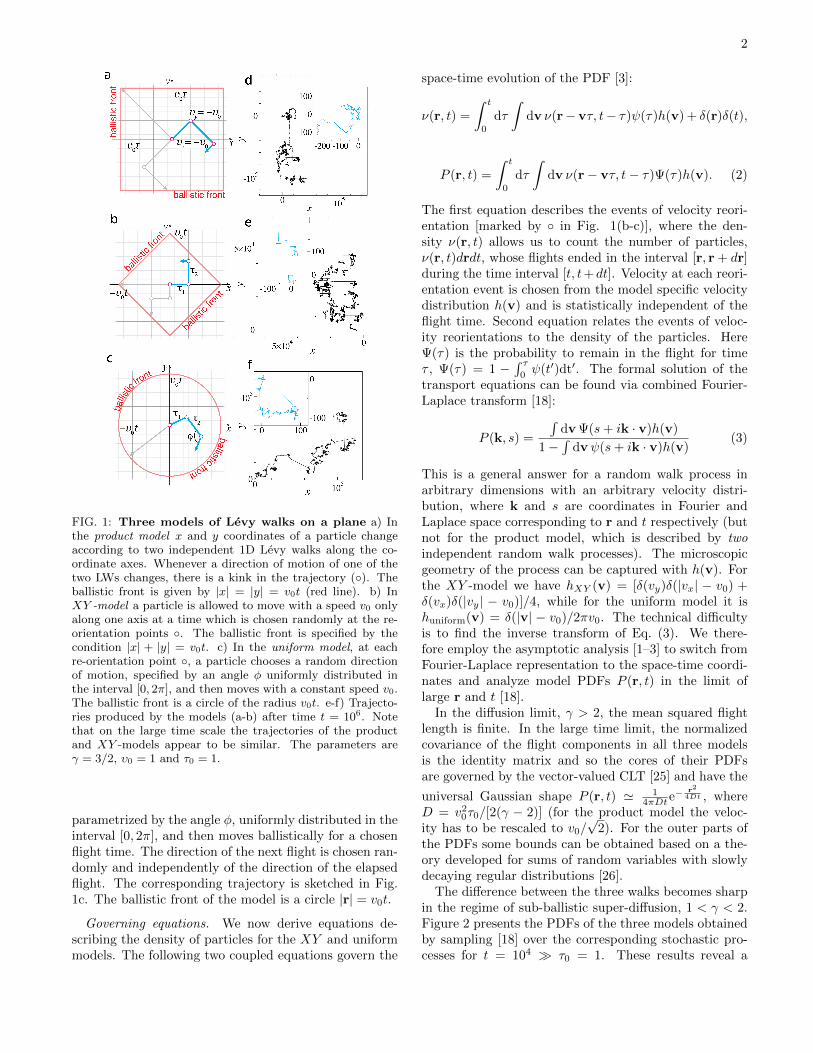
a) The simplest way to obtain two-dimensional Levywalk out of the one-dimensional one is to assume thatthe motions along each axis, x and y, are identical andindependent one-dimensional LW processes, as shownin Fig 1a. The two-dimensional PDF P (r, t), r(t) ={x(t), y(t)}, of this product model is given by the prod-uct of two one-dimensional LW PDFs, Pprod(r, t) =PLW(x, t) ·PLW(y, t). On the microscopic scale, each bal-listic event corresponds to the motion along either thediagonal or anti-diagonal. Every re-orientation only par-tially erases the memory about the last ballistic flight:while the direction of the motion along one axis could bechanged, the direction along the other axis almost surelyremains the same. The ballistic front has the shape of asquare with borders given by |x| = |y| = v0t.

b) In the XY-model, a particle is allowed to move onlyalong one of the axes at a time. A particle chooses arandom flight time τ from Eq. (1) and one out of fourdirections. Then it moves with a constant speed υ0 alongthe chosen direction. After the flight time is elapsed, anew random direction and a new flight time are chosen.This process is sketched in Fig. 1b. The ballistic front isa square defined by the equation |x|+ |y| = v0t.

c) The uniform model follows the original definitionby Pearson [17]. A particle chooses a random direction,

arX

iv:1

605.

0290

8v3

[co

nd-m

at.s

tat-

mec

h] 1

Jan

201

7

2

FIG. 1: Three models of Levy walks on a plane a) Inthe product model x and y coordinates of a particle changeaccording to two independent 1D Levy walks along the co-ordinate axes. Whenever a direction of motion of one of thetwo LWs changes, there is a kink in the trajectory (◦). Theballistic front is given by |x| = |y| = v0t (red line). b) InXY -model a particle is allowed to move with a speed v0 onlyalong one axis at a time which is chosen randomly at the re-orientation points ◦. The ballistic front is specified by thecondition |x| + |y| = v0t. c) In the uniform model, at eachre-orientation point ◦, a particle chooses a random directionof motion, specified by an angle φ uniformly distributed inthe interval [0, 2π], and then moves with a constant speed v0.The ballistic front is a circle of the radius v0t. e-f) Trajecto-ries produced by the models (a-b) after time t = 106. Notethat on the large time scale the trajectories of the productand XY -models appear to be similar. The parameters areγ = 3/2, υ0 = 1 and τ0 = 1.

parametrized by the angle φ, uniformly distributed in theinterval [0, 2π], and then moves ballistically for a chosenflight time. The direction of the next flight is chosen ran-domly and independently of the direction of the elapsedflight. The corresponding trajectory is sketched in Fig.1c. The ballistic front of the model is a circle |r| = v0t.

Governing equations. We now derive equations de-scribing the density of particles for the XY and uniformmodels. The following two coupled equations govern the

space-time evolution of the PDF [3]:

ν(r, t) =

∫ t

0

dτ

∫dv ν(r− vτ, t− τ)ψ(τ)h(v) + δ(r)δ(t),

P (r, t) =

∫ t

0

dτ

∫dv ν(r− vτ, t− τ)Ψ(τ)h(v). (2)

The first equation describes the events of velocity reori-entation [marked by ◦ in Fig. 1(b-c)], where the den-sity ν(r, t) allows us to count the number of particles,ν(r, t)drdt, whose flights ended in the interval [r, r + dr]during the time interval [t, t+dt]. Velocity at each reori-entation event is chosen from the model specific velocitydistribution h(v) and is statistically independent of theflight time. Second equation relates the events of veloc-ity reorientations to the density of the particles. HereΨ(τ) is the probability to remain in the flight for timeτ , Ψ(τ) = 1 −

∫ τ0ψ(t′)dt′. The formal solution of the

transport equations can be found via combined Fourier-Laplace transform [18]:

P (k, s) =

∫dvΨ(s+ ik · v)h(v)

1−∫

dvψ(s+ ik · v)h(v)(3)

This is a general answer for a random walk process inarbitrary dimensions with an arbitrary velocity distri-bution, where k and s are coordinates in Fourier andLaplace space corresponding to r and t respectively (butnot for the product model, which is described by twoindependent random walk processes). The microscopicgeometry of the process can be captured with h(v). Forthe XY -model we have hXY (v) = [δ(vy)δ(|vx| − v0) +δ(vx)δ(|vy| − v0)]/4, while for the uniform model it ishuniform(v) = δ(|v| − v0)/2πv0. The technical difficultyis to find the inverse transform of Eq. (3). We there-fore employ the asymptotic analysis [1–3] to switch fromFourier-Laplace representation to the space-time coordi-nates and analyze model PDFs P (r, t) in the limit oflarge r and t [18].

In the diffusion limit, γ > 2, the mean squared flightlength is finite. In the large time limit, the normalizedcovariance of the flight components in all three modelsis the identity matrix and so the cores of their PDFsare governed by the vector-valued CLT [25] and have the

universal Gaussian shape P (r, t) ' 14πDte

− r2

4Dt , whereD = v2

0τ0/[2(γ − 2)] (for the product model the veloc-ity has to be rescaled to v0/

√2). For the outer parts of

the PDFs some bounds can be obtained based on a the-ory developed for sums of random variables with slowlydecaying regular distributions [26].

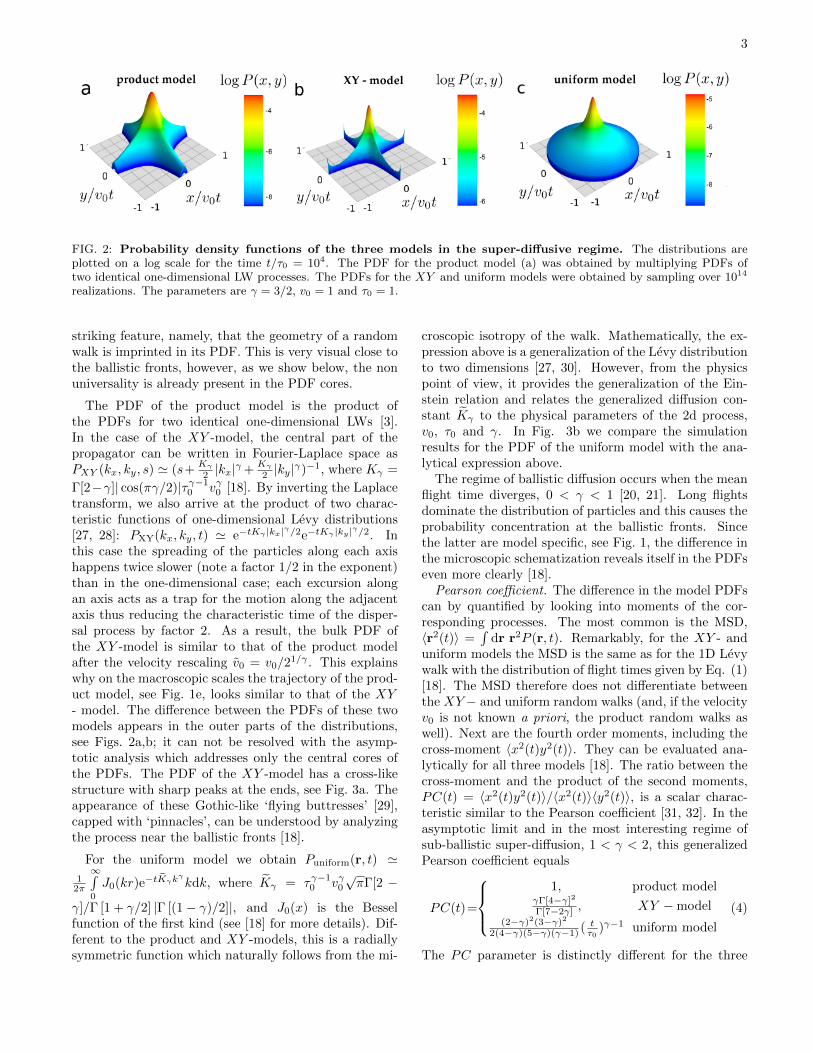
The difference between the three walks becomes sharpin the regime of sub-ballistic super-diffusion, 1 < γ < 2.Figure 2 presents the PDFs of the three models obtainedby sampling [18] over the corresponding stochastic pro-cesses for t = 104 � τ0 = 1. These results reveal a

3

FIG. 2: Probability density functions of the three models in the super-diffusive regime. The distributions areplotted on a log scale for the time t/τ0 = 104. The PDF for the product model (a) was obtained by multiplying PDFs oftwo identical one-dimensional LW processes. The PDFs for the XY and uniform models were obtained by sampling over 1014

realizations. The parameters are γ = 3/2, v0 = 1 and τ0 = 1.

striking feature, namely, that the geometry of a randomwalk is imprinted in its PDF. This is very visual close tothe ballistic fronts, however, as we show below, the nonuniversality is already present in the PDF cores.

The PDF of the product model is the product ofthe PDFs for two identical one-dimensional LWs [3].In the case of the XY -model, the central part of thepropagator can be written in Fourier-Laplace space asPXY (kx, ky, s) ' (s+

Kγ2 |kx|

γ +Kγ2 |ky|

γ)−1, where Kγ =

Γ[2−γ]| cos(πγ/2)|τγ−10 vγ0 [18]. By inverting the Laplace

transform, we also arrive at the product of two charac-teristic functions of one-dimensional Levy distributions[27, 28]: PXY(kx, ky, t) ' e−tKγ |kx|

γ/2e−tKγ |ky|γ/2. In

this case the spreading of the particles along each axishappens twice slower (note a factor 1/2 in the exponent)than in the one-dimensional case; each excursion alongan axis acts as a trap for the motion along the adjacentaxis thus reducing the characteristic time of the disper-sal process by factor 2. As a result, the bulk PDF ofthe XY -model is similar to that of the product modelafter the velocity rescaling v0 = v0/2

1/γ . This explainswhy on the macroscopic scales the trajectory of the prod-uct model, see Fig. 1e, looks similar to that of the XY- model. The difference between the PDFs of these twomodels appears in the outer parts of the distributions,see Figs. 2a,b; it can not be resolved with the asymp-totic analysis which addresses only the central cores ofthe PDFs. The PDF of the XY -model has a cross-likestructure with sharp peaks at the ends, see Fig. 3a. Theappearance of these Gothic-like ‘flying buttresses’ [29],capped with ‘pinnacles’, can be understood by analyzingthe process near the ballistic fronts [18].

For the uniform model we obtain Puniform(r, t) '1

2π

∞∫0

J0(kr)e−tKγkγ

kdk, where Kγ = τγ−10 vγ0

√πΓ[2 −

γ]/Γ [1 + γ/2] |Γ [(1− γ)/2]|, and J0(x) is the Besselfunction of the first kind (see [18] for more details). Dif-ferent to the product and XY -models, this is a radiallysymmetric function which naturally follows from the mi-

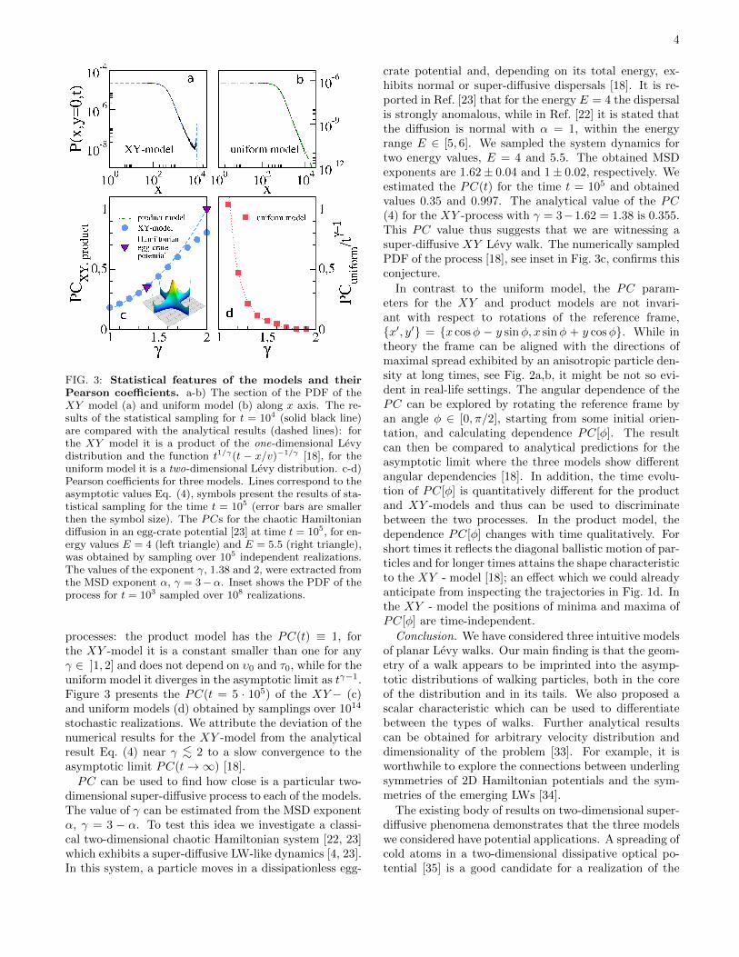
croscopic isotropy of the walk. Mathematically, the ex-pression above is a generalization of the Levy distributionto two dimensions [27, 30]. However, from the physicspoint of view, it provides the generalization of the Ein-stein relation and relates the generalized diffusion con-stant Kγ to the physical parameters of the 2d process,v0, τ0 and γ. In Fig. 3b we compare the simulationresults for the PDF of the uniform model with the ana-lytical expression above.

The regime of ballistic diffusion occurs when the meanflight time diverges, 0 < γ < 1 [20, 21]. Long flightsdominate the distribution of particles and this causes theprobability concentration at the ballistic fronts. Sincethe latter are model specific, see Fig. 1, the difference inthe microscopic schematization reveals itself in the PDFseven more clearly [18].

Pearson coefficient. The difference in the model PDFscan by quantified by looking into moments of the cor-responding processes. The most common is the MSD,〈r2(t)〉 =

∫dr r2P (r, t). Remarkably, for the XY - and

uniform models the MSD is the same as for the 1D Levywalk with the distribution of flight times given by Eq. (1)[18]. The MSD therefore does not differentiate betweenthe XY− and uniform random walks (and, if the velocityv0 is not known a priori, the product random walks aswell). Next are the fourth order moments, including thecross-moment 〈x2(t)y2(t)〉. They can be evaluated ana-lytically for all three models [18]. The ratio between thecross-moment and the product of the second moments,PC(t) = 〈x2(t)y2(t)〉/〈x2(t)〉〈y2(t)〉, is a scalar charac-teristic similar to the Pearson coefficient [31, 32]. In theasymptotic limit and in the most interesting regime ofsub-ballistic super-diffusion, 1 < γ < 2, this generalizedPearson coefficient equals

PC(t)=

1, product model

γΓ[4−γ]2

Γ[7−2γ] , XY −model(2−γ)2(3−γ)2

2(4−γ)(5−γ)(γ−1) ( tτ0

)γ−1 uniform model

(4)

The PC parameter is distinctly different for the three

4

FIG. 3: Statistical features of the models and theirPearson coefficients. a-b) The section of the PDF of theXY model (a) and uniform model (b) along x axis. The re-sults of the statistical sampling for t = 104 (solid black line)are compared with the analytical results (dashed lines): forthe XY model it is a product of the one-dimensional Levydistribution and the function t1/γ(t − x/v)−1/γ [18], for theuniform model it is a two-dimensional Levy distribution. c-d)Pearson coefficients for three models. Lines correspond to theasymptotic values Eq. (4), symbols present the results of sta-tistical sampling for the time t = 105 (error bars are smallerthen the symbol size). The PCs for the chaotic Hamiltoniandiffusion in an egg-crate potential [23] at time t = 105, for en-ergy values E = 4 (left triangle) and E = 5.5 (right triangle),was obtained by sampling over 105 independent realizations.The values of the exponent γ, 1.38 and 2, were extracted fromthe MSD exponent α, γ = 3−α. Inset shows the PDF of theprocess for t = 103 sampled over 108 realizations.

processes: the product model has the PC(t) ≡ 1, forthe XY -model it is a constant smaller than one for anyγ ∈ ]1, 2] and does not depend on υ0 and τ0, while for theuniform model it diverges in the asymptotic limit as tγ−1.Figure 3 presents the PC(t = 5 · 105) of the XY− (c)and uniform models (d) obtained by samplings over 1014

stochastic realizations. We attribute the deviation of thenumerical results for the XY -model from the analyticalresult Eq. (4) near γ <∼ 2 to a slow convergence to theasymptotic limit PC(t→∞) [18].PC can be used to find how close is a particular two-

dimensional super-diffusive process to each of the models.The value of γ can be estimated from the MSD exponentα, γ = 3 − α. To test this idea we investigate a classi-cal two-dimensional chaotic Hamiltonian system [22, 23]which exhibits a super-diffusive LW-like dynamics [4, 23].In this system, a particle moves in a dissipationless egg-

crate potential and, depending on its total energy, ex-hibits normal or super-diffusive dispersals [18]. It is re-ported in Ref. [23] that for the energy E = 4 the dispersalis strongly anomalous, while in Ref. [22] it is stated thatthe diffusion is normal with α = 1, within the energyrange E ∈ [5, 6]. We sampled the system dynamics fortwo energy values, E = 4 and 5.5. The obtained MSDexponents are 1.62± 0.04 and 1± 0.02, respectively. Weestimated the PC(t) for the time t = 105 and obtainedvalues 0.35 and 0.997. The analytical value of the PC(4) for the XY -process with γ = 3−1.62 = 1.38 is 0.355.This PC value thus suggests that we are witnessing asuper-diffusive XY Levy walk. The numerically sampledPDF of the process [18], see inset in Fig. 3c, confirms thisconjecture.

In contrast to the uniform model, the PC param-eters for the XY and product models are not invari-ant with respect to rotations of the reference frame,{x′, y′} = {x cosφ − y sinφ, x sinφ + y cosφ}. While intheory the frame can be aligned with the directions ofmaximal spread exhibited by an anisotropic particle den-sity at long times, see Fig. 2a,b, it might be not so evi-dent in real-life settings. The angular dependence of thePC can be explored by rotating the reference frame byan angle φ ∈ [0, π/2], starting from some initial orien-tation, and calculating dependence PC[φ]. The resultcan then be compared to analytical predictions for theasymptotic limit where the three models show differentangular dependencies [18]. In addition, the time evolu-tion of PC[φ] is quantitatively different for the productand XY -models and thus can be used to discriminatebetween the two processes. In the product model, thedependence PC[φ] changes with time qualitatively. Forshort times it reflects the diagonal ballistic motion of par-ticles and for longer times attains the shape characteristicto the XY - model [18]; an effect which we could alreadyanticipate from inspecting the trajectories in Fig. 1d. Inthe XY - model the positions of minima and maxima ofPC[φ] are time-independent.

Conclusion. We have considered three intuitive modelsof planar Levy walks. Our main finding is that the geom-etry of a walk appears to be imprinted into the asymp-totic distributions of walking particles, both in the coreof the distribution and in its tails. We also proposed ascalar characteristic which can be used to differentiatebetween the types of walks. Further analytical resultscan be obtained for arbitrary velocity distribution anddimensionality of the problem [33]. For example, it isworthwhile to explore the connections between underlingsymmetries of 2D Hamiltonian potentials and the sym-metries of the emerging LWs [34].

The existing body of results on two-dimensional super-diffusive phenomena demonstrates that the three modelswe considered have potential applications. A spreading ofcold atoms in a two-dimensional dissipative optical po-tential [35] is a good candidate for a realization of the

5

product model. Lorentz billiards [36–38] reproduce theXY Levy walk with exponent γ = 2. The uniform modelis relevant to the problems of foraging, motility of mi-croorganisms, and mobility of humans [3, 11, 12, 39, 40].On the physical side, the uniform model is relevant toa Levy-like super-diffusive motion of a gold nanoclusteron a plane of graphite [41] and a graphene flake placedon a graphene sheet [42]. LWs were also shown, undercertain conditions, to be the optimal strategy for search-ing random sparse targets [13, 43]. The performance ofsearchers using different types of 2D LWs (for example,under specific target arrangements) is a perspective topic[44]. Finally, it would be interesting to explore a non-universal behavior of systems driven by different types ofmulti-dimensional Levy noise [45–47].

This work was supported by the the Russian ScienceFoundation grant No. 16-12-10496 (VZ and SD). IF andEB acknowledge the support by the Israel Science Foun-dation.

[1] M. F. Shlesinger, J. Klafter, and Y. Wong, J. Stat. Phys.27, 499 (1982).

[2] M. F. Shlesinger, B. J. West, and J. Klafter, Phys. Rev.Lett. 58, 1100 (1987).

[3] V. Zaburdaev, S. Denisov, J. Klafter, Rev. Mod. Phys.87, 483 (2015).

[4] J. Klafter, M.F. Shlesinger, and G. Zumofen, Phys. To-day 49, 33 (1996).

[5] Y. Sagi, M. Brook, I. Almog, and N. Davidson, Phys.Rev. Lett. 108, 093002 (2012).

[6] T. H. Harris, E. J. Banigan, D. A. Christian, C. Konradt,E. D. Tait Wojno, K. Norose, E. H. Wilson, B. John, W.Weninger, A. D. Luster, A. J. Liu, and C. A. Hunter,Nature 486, 545 (2012).

[7] C. Ariel, A. Rabani, S. Benisty, J. D. Partridge, R. M.Harshey, and A. Be’er, Nature Comm. 6, 8396 (2015).

[8] D. A. Raichlen, B. M. Wood, A. D. Gordon, A. Z. P.Mabulla, F. W. Marlowe, H. Pontzer, Proc. Nat. Acad.Sci. USA 111, 728 (2014).

[9] G. M. Fricke, F. Asperti-Boursin, J. Hecker, J. Cannon,and M. Moses, Adv. Artif. Life ECAL 12, 1009 (2013).

[10] J. Beal, ACM Trans. Auton. Adapt. Syst. 10, 1 (2015).[11] V. Mendez, D. Campos, and F. Bartumeus, Stochas-

tic Foundations in Movementecology (Springer,Berlin/Heidelberg, 2014).

[12] G. Viswanathan, M. da Luz, E. Raposo, and H. Stanley,The Physics of Foraging: An Introduction to RandomSearches and Biological Encounters (Cambridge Univer-sity Press, 2011).

[13] O. Benichou, C. Loverdo, M. Moreau, and R. Voituriez,Rev. Mod. Phys. 83, 81 (2011).

[14] B. Gnedenko and A. Kolmogorov, Limit distributions forsums of independent random variables (Addison-Wesley,Reading, MA, 1954).

[15] F. Spitzer, Principles of Random Walks (Spriinger, NY,1976).

[16] J. Klafter and I.M. Sokolov, First Steps in Random Walks(Oxford University Press, 2011).

[17] K. Pearson, Nature 72, 294 (1905).[18] See Supplemental Material, which includes Refs. [19–24].[19] A. Erdelyi, Tables of Integral Transforms, Vol. 1

(McGraw-Hill, New York, 1954).[20] D. Froemberg, M. Schmiedeberg, E. Barkai, and V.

Zaburdaev, Phys. Rev. E 91, 022131 (2015).[21] M. Magdziarz, and T. Zorawik, Phys. Rev. E 94, 022130

(2016).[22] T. Geisel, A. Zacherl, and G. Radons G, Phys. Rev. Lett.

59, 2503 (1987).[23] J. Klafter and G. Zumofen, Phys. Rev. E 49, 4873 (1994).[24] J. Laskar, and P. Robutel, Celest. Mech. Dyn. Astron.

80, 39 (2001).[25] A. W. Van der Vaart, Asymptotic Statistics (Cambridge

University Press, 1998).[26] A. A. Borovkov and K. A. Borovkov, Asymptotic Analy-

sis of Random Walks: Heavy-tailed Distributions (Cam-bridge University Press, 2008).

[27] V. Uchaikin and V. Zolotarev, Chance and Stability: Sta-ble Distributions and their Applications, Modern Prob-ability and Statistics (De Gruyter, Berlin/New York,1999).

[28] A. A. Dubkov, B. Spagnolo, and V. V. Uchaikin, Intern.J. Bifurcat. Chaos, 18, 2649 (2008).

[29] J. Heyman, The Stone Skeleton (Cambridge UniversityPress, 1997).

[30] J. P. Taylor-King, R. Klages, S. Fedotov, and R. A. VanGorder, Phys. Rev. E 94, 012104 (2016).

[31] K. Pearson, Proc. Roy. Soc. London 58, 240 (1895).[32] J. F. Kenney and E. S. Keeping, Mathematics of Statis-

tics, Pt. 2 (Princeton, NJ:Van Nostrand, 1951).[33] I. Fouxon, S. Denisov, V. Zaburdaev, and E. Barkai,

http://www.mpipks-dresden.mpg.de/~denysov/

ubprfinal11.pdf.[34] G. M. Zaslavsky, M. Edelman, and B. A. Niyazov, Chaos

7, 159 (1997).[35] S. Marksteiner, K. Ellinger, and P. Zoller, Phys. Rev. A

53, 3409 (1996).[36] Ya. G. Sinai, Russ. Math. Surveys 25, 137 (1970).[37] J.-P. Bouchaud and A. Georges A, Phys. Rep. 195, 127

(1990).[38] G. Cristadoro, T. Gilbert, M. Lenci, D. P. Sanders, Phys.

Rev. E 90, 050102 (2014).[39] N. E. Humphries, H. Weimerskirch, and D. W. Sims,

Methods Ecol. Evol. 4, 930 (2013).[40] G. C. Hays, T. Bastian, T. K. Doyle, S. Fossette, A. C.

Gleiss, M. B. Gravenor, V. J. Hobson, N. E. Humphries,M. K. S. Lilley, N. G. Pade, and D. W. Sims, Proc. R.Soc. B 279, 465 (2012).

[41] W. D. Luedtke and U. Landamn, Phys. Rev. Lett. 82,3835 (1999).

[42] T. V. Lebedeva et al., Phys. Rev. B 82, 155460 (2010).[43] G. M. Viswanathan, S. V. Buldyrev, S. Havlin, M. G. E.

da Luz, E. P. Raposo, and H. E. Stanley, Nature 401,911 (1999).

[44] M. Chupeau, O. Benichou, and R. Voituriez, NaturePhys. 11, 844 (2015).

[45] A. La Cognata, D. Valenti, A. A. Dubkov, and B. Spag-nolo, Phys. Rev. E 82, 011121 (2010).

[46] C. Guarcello, D. Valenti, A. Carollo, B. Spagnolo, J. Stat.Mech. Theor. Exp. 054012 (2016).

[47] D. Valenti, C. Guarcello, B. Spagnolo, Phys. Rev. B 89,214510 (2014).

6

SUPPLEMENTAL MATERIAL

Probability density functions of 2D Levy walks: general solution

The main mathematical tool we use to resolve the integral transport equations is the combined Fourier-Laplacetransform with respect to space and time, defined as:

f(k, s) =

∞∫0

dt

∫dr e−ikre−stf(r, t). (S1)

The coordinates in Fourier and Laplace spaces are k and s respectively. The corresponding inverse transform isdefined in the standard way [S1]. In the text and in the following we omit the hat sign and distinguish transformedfunctions by their arguments.

To find a solution to the system in Eq. (2) in the main text, we apply Fourier-Laplace transform, use its shiftproperty, ∫

dr e−ikrf(r− a) = e−ikaf(k);

∞∫0

dt e−ste−atf(t) = f(s+ a). (S2)

and obtain:

ν(k, s) = ν(k, s)

∫dvψ(s+ ikv)h(v) + 1, (S3)

P (k, s) = ν(k, s)

∫dvΨ(s+ ikv)h(v). (S4)

A system of integral equations in normal coordinates and time is reduced to a system of two linear equations forFourier-Laplace transformed functions; it is easily resolved to give Eq. (3):

P (k, s) =

∫dvΨ(s+ ikv)h(v)

1−∫

dvψ(s+ ikv)h(v)(S5)

It is important to note that this answer is valid for both XY - and uniform models, but not for the product model.The technical difficulty of finding the inverse Fourier-Laplace transform is the coupled nature of the problem, where

space and time enter the same argument. One way to address the problem is to do asymptotic analysis. Instead oflooking at full transformed functions we may consider their expansions with respect to small k, s, corresponding tolarge space and time scales in the normal coordinates. There are two such functions in the general answer Eq. (3) inthe main text, ψ(s+ikv) and Ψ(s+ikv) (note that those are Laplace transforms only, where the Fourier coordinate kenters the same argument together with s). In fact their Laplace transforms are related Ψ(s) = [1−ψ(s)]/s, thereforeit is sufficient to show the asymptotic expansion of ψ(s) for a small argument:

ψ(s+ ikv) ' 1 − τ0γ − 1

(s+ ikv)− τγ0 Γ[1− γ](s+ ikv)γ

+τ20

(γ − 2)(γ − 1)(s+ ikv)2 + .... (S6)

Depending on the value of γ different terms have the dominating role in this expansion. Such for γ > 2 zeroth, firstand second order terms are dominant, leading to the classical diffusion. In the intermediate regime 1 < γ < 2 zeroth,linear and a term with a fractional power of s+ ikv are dominant and lead to the Levy distribution.

Now by using this asymptotic expansions we can express the propagators. For example, the propagator of theuniform model in the sub-ballistic regime, after integration with respect to h(v), has the asymptotic form:

Puniform(k, s) ' 1

s+ |k|γ τγ−10 vγ0

√πΓ[2−γ]

Γ[1+γ/2]|Γ[(1−γ)/2]|

. (S7)

The inverse Laplace of this expression yields an exponential function, and an additional inverse Fourier transform inpolar coordinates leads to the 2D Levy distribution discussed in the main text.

7

We can also write down a similar asymptotic result for the central part of the PDF in the sub-ballistic regime1 < γ < 2 for arbitrary (but symmetric) velocity distribution h(v) = h(−v), for arbitrary dimension d:

P (r, t) '∫

exp[ik · r− tA

∣∣∣cos(πγ

2

)∣∣∣ 〈|k · v|γ〉] dk

(2π)d. (S8)

where A = (τ0)γ−1Γ[2 − γ]. The spatial statistics P (r, t) is controlled by the average over the velocity PDF via afunction 〈|k · v|γ〉 which depends on the direction of k. This is very different from the Gaussian case where only thecovariance matrix of the velocities enters in the asymptotic limit of P (r, t). In this sense the PDF of Levy walksEq. (S8) is non-universal if compared with one dimensional Levy walks, or normal d dimensional diffusion.

Difference between the XY and product models in the sub-ballistic regime

The asymptotic analysis shows that in the bulk, the XY model is identical to the product model. Therefore thecross-section of the XY PDF along the x (or y) axis is well approximated by the standard 1D Levy distribution (seeFig. 3a,b), similarly to the product model. There is, however, a significant deviation at the tail close to the ballisticfront. Let us look at the XY model closer to the front. Consider the density on the x axis, at some point x <∼ vt. Ifa particle is that far on x axis, it means that this particle had spent at most time ty = t− x/v for its walks along they direction. Therefore, if we look at the PDF along the y direction, it has been ’built’ by only those particles whichspend time ty evolving along this direction (note that for the product model the time of walks along both directionsis the same t as both walks are independent). Therefore, for a given moment of time, the PDF along x-axis of theXY model is not the 1D Levy distribution uniformly scaled with the pre-factor 1/t1/γ (as in the product model) buta product of the Levy distribution and the non-homogeneous factor t1/γ/(t− x/v)1/γ ; this pre-factor diverges as theparticle gets closer to the front (see Fig. 3a) but it is integrable, so that the total number of particles is still conserved.

Probability density functions of 2D Levy walks in the ballistic regime

For the product model, the PDF is given by the product of two PDFs of the one-dimensional Levy walk. In theballistic regime, PDF of the Levy walk is the Lamperti distribution [S2]. For some particular values of γ it has a

compact form. For example, for γ = 1/2 we have P(γ=1/2)LW (x, t) = π−1(v2

0t2 − x2)−1/2, and therefore, for 2D we get

P(γ=1/2)prod (x, y, t) =

1

π2(v20t

2 − x2)1/2(v20t

2 − y2)1/2. (S9)

For the XY -model, the asymptotic expression for the propagator in the ballistic regime 0 < γ < 1 is

PXY (kx, ky, s) =(s+ ikxv0)γ−1 + (s− ikxv0)γ−1 + (s+ ikyv0)γ−1 + (s− ikyv0)γ−1

(s+ ikxv0)γ + (s− ikxv0)γ + (s+ ikyv0)γ + (s− ikyv0)γ. (S10)

For the uniform model, the answer is more compact:

Puniform(k, s) =

∫ 2π

0(s+ ikv0 cosϕ)γ−1dϕ∫ 2π

0(s+ ikv0 cosϕ)γdϕ

, (S11)

where k = |k|. The integrals over the angle ϕ can be calculated yielding hyper-geometric functions; the remainingtechnical difficulty is to calculate the inverse transforms. Recently, it was shown in the one-dimensional case, that thepropagators of the ballistic regime can be calculated without explicitly performing the inverse transforms [S2]. Thisapproach has been then generalized to 2D case for the uniform model [S3], where the density of particles was shownto be described by the following expression:

P (r, t)uniform = − 1

π3/2t2D

1/2−

{ 1

x1/2Im

2F1((1− γ)/2, 1− γ/2; 1; 1x )

2F1(−γ/2, (1− γ)/2; 1; 1x )

}(r2

t2

)(S12)

where D1/2− is the right-side Riemann-Liouville fractional derivative of order 1/2 (see [S3] for further details). It would

be interesting to try to extend this formalism to random walks without rotational symmetry, such as for example theXY model. The PDFs for the three models in the ballistic regime are shown in Fig. S1.

8

FIG. S1: Probability density functions of the three models in the ballistic regime. The PDFs for the (a) productmodel, (b) XY -model, and (c) uniform model are plotted on a log scale (color bars are not shown) for the time t/τ0 = 104.The parameters are γ = 1/2, τ0 = v0 = 1.

FIG. S2: Second and forth moments of the three models in the super-diffusive regime, γ = 3/2. (left panel)The MSD is identical for all three models (though the product model needs an additional prefactor of 1/2). (right panel) Thedifference between the models becomes apparent in the cross-moment 〈x2y2〉. It scales as t6−2γ for the product and XY -modeland ad t5−γ for the uniform model. The inset shows that the convergence of the ration between the moments to the analyticalPC value (see Table S1) in course of time (number of realizations is 105 at every time point). The parameters are τ0 = v0 = 1.

MSD and higher moments

In case of an unbiased random walk that starts at zero, the MSD is defined as

⟨r2(t)

⟩=

∫dr r2P (r, t), (S13)

9

Moment 〈r2〉 〈x4〉 = 〈y4〉 〈x2y2〉 PC

Product4v20τ

γ−10 (γ−1)

(2−γ)(3−γ)t3−γ

4v40τγ−10 (γ−1)

(4−γ)(5−γ)t5−γ

4v40τ2γ−20 (γ−1)2

(2−γ)2(3−γ)2t6−2γ 1

XY2v20τ

γ−10 (γ−1)

(2−γ)(3−γ)t3−γ

2v40τγ−10 (γ−1)

(4−γ)(5−γ)t5−γ

v40τ2γ−20 γ(γ−1)4Γ2[1−γ]

Γ[7−2γ]t6−2γ γΓ[4−γ]2

Γ[7−2γ]

Uniform2v20τ

γ−10 (γ−1)

(2−γ)(3−γ)t3−γ

3v40τγ−10 (γ−1)

2(4−γ)(5−γ)t5−γ

v40τγ−10 (γ−1)

2(4−γ)(5−γ)t5−γ (γ−3)2(γ−2)2

2(5−γ)(4−γ)(γ−1)( tτ0

)γ−1

TABLE I: Asymptotic moments of the models.

The asymptotic behavior of the MSD can be calculated by differentiating the PDF in Fourier-Laplace space twicewith respect to k and afterwards setting k = 0.⟨

r2(t)⟩

= −∇2k P (k, t)|k=0 . (S14)

In fact we can see from Eq. (S5) that ∇k applied to P (k, s) is equivalent to −iv dds . Therefore all terms with the first

order derivatives disappear due to the integration with a symmetric velocity distribution. Only the terms with secondderivatives contribute to the answer:

−∇2kP (k, s)

∣∣k=0

=

∫dv v2h(v)

{Ψ(s) · ψ′′(s)[1− ψ(s)]2

+Ψ′′(s)

1− ψ(s)

}(S15)

Now, to calculate the scaling of the MSD in real time for different regimes of diffusion, we need to take the corre-sponding expansions of ψ(s) and Ψ(s) for small s, Eq. (S6), and perform the inverse Laplace transform. As a resultwe obtain

⟨r2(t)

⟩=

v2

0(1− γ)t2 0 < γ < 1

2v20τγ−10 (γ−1)

(3−γ)(2−γ) t3−γ 1 < γ < 2

2v20τ0γ−2 t γ > 2

(S16)

It is remarkable that for 0 < γ < 1 the scaling exponent of the MSD is independent of the tail exponent γ of theflight time distribution. An important observation is that the models are indistinguishable on the basis of their MSDbehavior, see Fig S2 (left panel). Similarly, we compute the forth moment and find that they scale similarly forall three models (though the prefactors are model-specific, see second column in Table S1). The difference betweenthe models become tangible in the cross-moments 〈x2y2〉. We use these moments to define a generalized Pearsoncoefficient which is denoted by PC,

PC(t) =〈x2(t)y2(t)〉〈x2(t)〉〈y2(t)〉

. (S17)

We concentrate on the sub-ballistic super-diffusive regime and summarize the corresponding results in Table S1.

Angular dependence of the Pearson coefficient

As mentioned in the main text, the value of PC depends on the choice of the coordinate frame. To quantify thedependence of the PC on the orientation of the frame of references we consider random walks {x′(t), y′(t)} which areobtained by turning three original random walks (uniform, product and XY ) by an arbitrary angle 0 ≤ φ ≤ π/2 withrespect to the x-axis and calculate the corresponding PC[φ]. The coordinates in the turned and original frames arerelated via:

{x′(t), y′(t)} = {x(t) cosφ− y(t) sinφ, x(t) sinφ+ y(t) cosφ)} (S18)

10

FIG. S3: Frame dependence and time evolution of the Pearson coefficient. a) Dependence of the Pearson coefficienton the frame orientation angle φ for the three models in the long-time limit. Symbols correspond to the results of the statisticalsampling for t = 105 and lines present analytical results for the asymptotic limit, Eq. S19. b-c) Time dependence of PC[φ] forthe product and XY models. For the short times, t <∼ 102, minima of the Pearson coefficient for the product model correspond

to the diagonal and anti-diagonal directions while for larger times, t > 102, these directions correspond to the maxima; minimaare attained along the {x, y} axes, see Fig. 1d in the main text. For the XY model the positions of maxima and minima aretime-independent. The parameters are the same as in Fig. 2 in the main text. Note that the mean time of ballistic flights is〈τ〉 = 2 for the chosen set of parameters.

After simple algebra and by discarding terms with odd powers of x and y, which will disappear after averaging dueto symmetry, we obtain:

PC[φ] =〈x2y2〉(cos4 φ+ sin4 φ− sin2 2φ) + (〈x4〉+ 〈y4〉) cos2 φ sin2 φ

〈x2y2〉(cos4 φ+ sin4 φ) + (〈x2〉2 + 〈y2〉2) cos2 φ sin2 φ. (S19)

This expression can now be evaluated by using the fourth and second-order cross moments of the original random walksgiven in Table S1. It can be shown that for the product and XY models and for any φ 6= {0, π/2}, PC(t;φ) ∝ tγ−1,whereas for the uniform model PC(t;φ) ∝ tγ−1 is naturally independent of the angle φ. The angle dependent Pearsoncoefficients are different for all three models, see Fig. S3a. Importantly, the Pearson coefficient contains only one“unknown” parameter τ0, the scaling parameter of the flight time PDF (recall that the exponent γ of the power lawtail in the flight time distribution can be determined from the scaling of the MSD). Thus by measuring the PC(t;φ),for example, at two different time points would allow for a unambiguous determination of τ0 and of the type of therandom walk model.

An interesting observation can be made by numerically calculating PC[φ] as a function of time. While the shapeof the dependence remains the same for the uniform- (flat at any time) and XY -model (see Fig.S3c), for the productmodel it changes qualitatively. The minima of the PCprod(t;φ) for short times transform into the maxima for largetimes passing through an intermediate flat shape, see Fig. S3b. This is a quantification of the transition we alsoobserve by sampling individual trajectories. It is a consequence of the fact that for short times the preferred directionof motion are diagonals and anti-diagonals (inset in Fig.1d), whereas for large times the trajectories resemble those ofthe XY -model (Fig. 1d,e). Correspondingly the maximum of the PC[φ] “shifts” by π/4 as time progresses. At thesame time, the positions of maxima and minima of PC[φ] for the XY model are time-invariant. This effect can beused to distinguish between the two models.

11

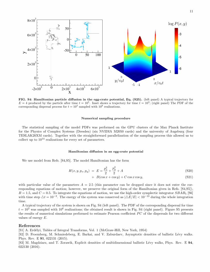
FIG. S4: Hamiltonian particle diffusion in the egg-crate potential, Eq. (S25). (left panel) A typical trajectory forE = 4 produced by the particle after time t = 105. Inset shows a trajectory for time t = 103; (right panel) The PDF of thecorresponding dispersal process for t = 103 sampled with 108 realizations.

Numerical sampling procedure

The statistical sampling of the model PDFs was performed on the GPU clusters of the Max Planck Institutefor the Physics of Complex Systems (Dresden) (six NVIDIA M2050 cards) and the university of Augsburg (fourTESLAK20XM cards). Together with the straightforward parallelization of the sampling process this allowed us tocollect up to 1014 realizations for every set of parameters.

Hamiltonian diffusion in an egg-crate potential

We use model from Refs. [S4,S5]. The model Hamiltonian has the form

H(x, y, px, py) = E =p2x

2+p2y

2+A (S20)

+ B(cosx+ cos y) + C cosx cos y, (S21)

with particular value of the parameters A = 2.5 (this parameter can be dropped since it does not enter the cor-responding equations of motion; however, we preserve the original form of the Hamiltonian given in Refs. [S4,S5]),B = 1.5, and C = 0.5. To integrate the equations of motion, we use the high-order symplectic integrator SBAB5 [S6]with time step 4t = 10−3. The energy of the system was conserved as |4E/E| < 10−10 during the whole integrationtime.

A typical trajectory of the system is shown on Fig. S4 (left panel). The PDF of the corresponding dispersal for timet = 103 was sampled with 108 realizations; the obtained result is shown in Fig. S4 (right panel). Figure S5 presentsthe results of numerical simulations performed to estimate Pearson coefficient PC of the dispersals for two differentvalues of energy E.

References[S1] A. Erdelyi, Tables of Integral Transforms, Vol. 1 (McGraw-Hill, New York, 1954)[S2] D. Froemberg, M. Schmiedeberg, E. Barkai, and V. Zaburdaev, Asymptotic densities of ballistic Levy walks.Phys. Rev. E 91, 022131 (2015).[S3] M. Magdziarz, and T. Zorawik, Explicit densities of multidimensional ballistic Levy walks, Phys. Rev. E 94,022130 (2016).

12

[S4] T. Geisel, A. Zacherl, and G. Radons, Generic 1/f noise in chaotic Hamiltonian dynamics. Phys. Rev. Lett. 59,2503–2506 (1987).[S5] J. Klafter and G. Zumofen, Levy statistics in a Hamiltonian system. Phys. Rev. E 49, 4873–4877 (1994).[S6] J. Laskar, and P. Robutel, High order sympletic integrators for perturbed Hamiltonian systems. Celest. Mech.Dyn. Astron. 80, 39 (2001).

FIG. S5: Pearson coefficient and moment scaling for the Hamiltonian dispersal. PCs of the dispersals for twoenergy values were sampled (left panel). Plot shows Pearson coefficients for the fixed time t = 105 as a function of numberof collected realizations. Thin dashed lines correspond to the analytical results, Tabe S1, obtained for exponents γ extractedfrom the MSD of the dispersals (right panel).