Supersonic Shock in Gas Bearings

1. Introduction

A complete and correct analysis of the pressure distribution in a compressible fluid film must include a

treatment of supersonic flow. Although flows may accelerate gradually and isentropically from

subsonic to supersonic velocities, the reverse is rarely true. In a diverging flow path, the velocity of a

supersonic flow continually increases, but cannot increase indefinitely. Eventually, the energy becomes

too widely dispersed to maintain ever-higher velocities and a transition to subsonic flow ensues.

This transition is abrupt and irreversible, and is called a normal shock, ‘normal’ meaning perpendicular

to the direction of flow lines. The normal shock is stationary relative to the flow boundaries, and thus is

also described as a standing shock wave. The static pressure of a gas varies dramatically depending on

whether its velocity is above or below the speed of sound, making the existence and location of normal

shocks of primary importance to hydrostatic gas bearing designers.

This report will describe the equations and procedures needed to determine the location of a shock wave,

the size of the supersonic flow region, and the complete pressure distribution in an externally

pressurized gas bearing clearance.

Nomenclature

Ax area normal to flow at point x

Cd ad hoc orifice discharge coefficient

D recess diameter

d recess depth

K integral gain for iterative solutions

k ratio of specific heats cp/cv, equal to 1.4 for air

M Mach number

Mx Mach number at point x

p static pressure

px static pressure at point x

pS supply pressure

pt total pressure (isentropic stagnation or reference pressure)

ptx total pressure at point x

r radial variable, distance from gas inlet

R specific gas constant, equal to 287 Nm/(kgK) for air

R pressure ratio p/pt

Rx pressure ratio at point x

T temperature

TS supply temperature

Tx temperature at point x

Tt total temperature (isentropic stagnation or reference temperature)

Ttx total temperature at point x

V fluid velocity

Vr radial component of fluid velocity

w mass flow rate

z vertical cylindrical coordinate

α total flow number

µ absolute (dynamic) viscosity

ρ density

Γ normalized gas dynamics number

Γx normalized gas dynamics number at point x

The Gas Dynamics Approach Many analyses of externally pressurized gas bearings give only a cursory nod to the compressibility of

the fluid, and proceed with what is essentially a viscous, incompressible approach. The essential feature

of compressible flow is that a specified mass flow rate does not fully specify the velocity of the flow.

By analogy, cars moving past a fixed point in traffic may be close together and moving slowly, or

spaced farther apart and moving rapidly, yet the number of cars per unit time can be the same in both

cases. Static pressure in a gas film is strongly dependent on the velocity of the gas. Since conventional

approaches based on incompressible, viscous flow cannot account for the possibility of supersonic flow,

they cannot accurately predict the static pressure of the gas film. By extension, the load-carrying

capacity of the bearing cannot be accurately predicted [1].

This approach begins with a view of the crucial area immediately surrounding the point at which fluid

enters the bearing clearance. This flow may be treated as a one-dimensional radial flow. The cross-

sectional area normal to the flow is 2πrh where r is the radial distance from the inlet and h is the

(approximately constant) clearance surrounding the inlet. Even as the flow reaches the axial margins of

the bearing, or if significant recesses exist around the inlet, the flow may be treated as one-dimensional,

in which it is only required to specify the total cross-sectional area locally perpendicular to flow lines at

any place along the flow path (see Fig. 1).

This circular region around the inlet is the most critical, since it is responsible for a disproportionate

share of the bearing’s load capacity. This is the region in which the highest static pressure is expected to

occur, since the pressure is expected to approach the ambient pressure at points approaching the exit. If

the flow in this region is supersonic, the static pressure may be a mere fraction of the assumed pressure,

computed using viscous, incompressible models. Therefore, for purposes of both designing effective

gas bearings and analyzing bearing performance, a correct compressible fluid flow approach must be

used. This includes allowing for the possibility of supersonic flow, but also accounts for any reduction

in static pressure due to the velocity of the fluid, whether subsonic or supersonic.

Compressible Flow Theory

Refer to [2] for derivations of gas dynamics expressions. Most analyses of compressible flow assume a

fixed inlet pressure and variable backpressure at the outlet. Therefore, extra steps are required to

describe the more realistic case of a fixed outlet pressure (atmospheric) and variable supply pressure.

The three so-called “critical pressures” usually refer to the outlet pressures at which the flow through a

nozzle fundamentally changes character, assuming a fixed supply. In this report, the meaning of

“critical pressure” is altered to mean the supply pressure relative to a fixed exhaust that results in the

critical condition.

In quantifying the flow, neither velocity nor mass flow rate are sufficient, since each is a function of the

fluid’s pressure and temperature. The Mach number is used to properly take account of both the

thermodynamic and fluid dynamic state of the compressible flow:

kRT

V=M . (1)

The same information is conveyed by the pressure ratio R (not “plain” R, the specific gas constant),

defined as the ratio of static pressure to total pressure at a point in the flow:

tp

p=R . (2)

Total pressure is also known as the isentropic stagnation pressure or the isentropic reference pressure,

since it is the hypothetical static pressure that would exist if the flow were brought isentropically to a

complete stop from that point. The relationship between M and R (which is bounded by 0 and unity) is

Figure 1. Radial 1-D flow in the clearance.

kk

k −

−+=

12

2

11 MR (3)

and the inverse,

−

−=

−

11

21

2 k

k

kRM (4)

Specific values of M and R are valid only for one point in the flow path at a time. The Normalized Gas

Dynamics Function Γ and the Generalized Gas Dynamics Equation are needed to relate any two points

in a general compressible fluid flow. Γ is defined in terms of M and R by:

( )12

1

2

21

12

12

2

11

1

2

1

1

1

2 −+

−

+

−+

+

=

+

−

+

−=Γ

kk

k

kk

k

k

kk

k

kM

MRR. (5)

The Generalized Gas Dynamics Equation is:

21

2

1

2

1

21

1

2 Γ=Γ

A

A

p

p

T

T

t

t

t

t. (6)

This equation is valid for any one-dimensional steady flow of an ideal gas. In this report it will be

applied to the flow of a compressible fluid through an externally pressurized fluid film bearing. The

flow path is modeled as a one-dimensional passage with variable area. The supply is initially stagnant,

and passes through a restriction upon entering the clearance. In the clearance the fluid expands radially

until exiting to ambient conditions, as suggested in Fig. 1. This model represents a converging-

diverging nozzle geometry, which has been thoroughly treated in engineering texts.

Limiting Assumptions

Initially an assumption is made that past the restriction, the normal cross-sectional area of the flow path

only increases monotonically. This is not a realistic assumption to make when attempting to model a

real bearing, since bearing geometry invariably creates a secondary inherent restriction for flow entering

the clearance. An analysis of real geometries will be given later, but for now it is necessary to develop

the methods for solving gas dynamics problems on simpler models.

The flow will also be assumed isentropic to begin with. This is also an unrealistic assumption, as will be

demonstrated below, and the analysis will be extended once the simpler case has been developed.

It is also necessary to mention orifice loss coefficients. To begin with, the discharge coefficient will be

neglected. It will be introduced when we discuss breaking the isentropic assumption, and allowing

anisentropic flow, e.g. turbulence, viscous shearing, and normal shocks. The true nature of an orifice

discharge coefficient appears to be the rise in entropy due to the shock wave invariably associated with a

deceleration from sonic to subsonic flow as fluid leaves the orifice. Turbulence due to the sudden area

change also increases entropy.

It should be recognized that although often assumed to be constant, the orifice discharge coefficient

varies greatly with conditions. For example, below the first critical condition the discharge coefficient is

mainly the result of turbulence and viscosity. At choked flow conditions and above, normal shocks at

the orifice exit produce the effect, and the size of the effect depends on the strength of the shock.

For the first simplified set of assumptions described above, no discharge coefficient will be used. The

rational for this decision is that the normal shocks that are the focus of this analysis will take account of

the rise in entropy, making orifice coefficients redundant. In some cases, the orifice shock may exist

very close to the orifice exit, and secondary normal shocks in the clearance are sought. In such cases, an

orifice discharge coefficient will be assumed. Later, a method of computing the value of this coefficient

will be discussed.

A Note on Entropy

The concept of entropy is used extensively in the study of gas dynamics because it precisely summarized

a variety of related processes. In general terms, entropy is a measure of the distribution of energy in a

system. The absolute value of entropy is of no concern; rather it is the changes in entropy that matter.

When energy becomes more diffuse in a system, entropy rises. A rise in entropy accounts for an entire

class of processes known as ‘irreversible’ processes that can occur in fluids. Among these, of interest

here, are friction, viscous shearing, turbulence and shock waves. In this report, the phrase “entropy rise”

is used to indicate the presence of friction, viscosity, turbulence or shocks in the flow which tend to

increase the pressure drop in the flow, all else being equal. An isentropic (i.e. ‘equal entropy’) flow or

process indicates a situation in which none of those things are present, or are considered negligible. Any

anisentropic process has significant contributions from one or more irreversible effects.

Real flows are always anisentropic, but it is helpful, and sometimes necessary, to neglect irreversible

parts of a model for the sake of obtaining a meaningful analysis.

2. Critical Pressures

Three critical pressures or conditions exist in the analysis of converging-diverging gas flow. Only two

are directly applicable to hydrostatic bearing design, but values for all three critical pressures should be

computed when analyzing a bearing design.

The first critical describes the condition in which flow just reaches Mach 1 in the throat (the smallest

area in the passage) but is subsonic everywhere else in the flow. Supply pressures below this critical (or

exit pressures above the critical) result in subsonic flow even at the throat. Supply pressures above the

first critical result in a continued rise in mass flow through the throat, though the Mach number remains

unity there. The flow accelerates to supersonic levels beyond the throat until it drops abruptly down to

subsonic speed through a normal shock somewhere in the diverging section. Exit pressures below the

critical do not result in increased mass flow rate (the throat is “choked”) but produce the same shock

behavior in the diverging section.

The second critical condition occurs when the normal shock just reaches the exit of the diverging

section. In bearing applications, this represents the condition of having supersonic flow throughout the

clearance.

Between the second and third critical points, an oblique shock forms outside the exit because the fluid

leaves the nozzle at a static pressure lower than the exit pressure and makes the adjustment abruptly.

The exit pressure must be further lowered (or the supply raised) for all shocks to be eliminated.

The third critical condition, the desirable design point for rocket nozzles, represent completely isentropic

flow in the nozzle, i.e. no shock waves in or out of the diverging section. Supersonic flow continues

beyond the nozzle exit and diffuses without a shock wave. Flow beyond the second critical is not

thought to have any significance to bearing applications.

First Critical

The first critical designates the lowest supply (or highest exit) pressure resulting in choked flow (i.e. M

= 1) at the throat. To find the first critical supply pressure, one assumes a stagnant supply to begin with,

so that supply pressure pS is identified as the initial isentropic stagnation reference pressure, pt1, referred

to hereafter as total pressure. (See Fig. 2 for notation.) The flow is assumed to accelerate isentropically

from stagnant conditions to the speed of sound at the throat, so

Stt ppp == 12 . (7)

Sonic flow through the throat implies that Mach number at the throat, M2, is identically 1, and Γ2 = 1

from Eq. 5. The pressure ratio at the throat R2 is the critical pressure ratio, which for air (k = 1.4) is

0.5283 (using Eq. 3 with M = 1). This allows us to relate the static pressure at position 2 to the supply

pressure:

Figure 2. Flow path profile and notation.

1 2 3 4

F low

SSt pppp 5283.0 2222 === RR . (8)

If the supply pressure and temperature are known, Eq. 8 can be used to compute the mass flow rate or

the linear velocity. To find the unknown critical supply pressure, however, one must analyze the

divergent section past the throat. Note also that under the choked condition, the throat pressure, and

therefore the velocity and mass flow rate, is completely independent of the exit pressure.

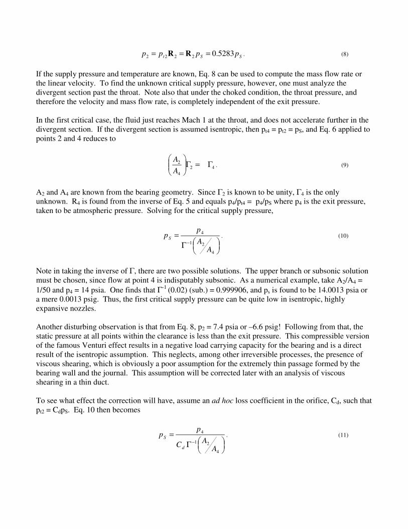
In the first critical case, the fluid just reaches Mach 1 at the throat, and does not accelerate further in the

divergent section. If the divergent section is assumed isentropic, then pt4 = pt2 = pS, and Eq. 6 applied to

points 2 and 4 reduces to

42

4

2 Γ=Γ

A

A. (9)

A2 and A4 are known from the bearing geometry. Since Γ2 is known to be unity, Γ4 is the only

unknown. R4 is found from the inverse of Eq. 5 and equals p4/pt4 = p4/pS where p4 is the exit pressure,

taken to be atmospheric pressure. Solving for the critical supply pressure,

Γ

=−

4

21

4

AA

ppS . (10)

Note in taking the inverse of Γ, there are two possible solutions. The upper branch or subsonic solution

must be chosen, since flow at point 4 is indisputably subsonic. As a numerical example, take A2/A4 =

1/50 and p4 = 14 psia. One finds that Γ-1 (0.02) (sub.) = 0.999906, and ps is found to be 14.0013 psia or

a mere 0.0013 psig. Thus, the first critical supply pressure can be quite low in isentropic, highly

expansive nozzles.

Another disturbing observation is that from Eq. 8, p2 = 7.4 psia or –6.6 psig! Following from that, the

static pressure at all points within the clearance is less than the exit pressure. This compressible version

of the famous Venturi effect results in a negative load carrying capacity for the bearing and is a direct

result of the isentropic assumption. This neglects, among other irreversible processes, the presence of

viscous shearing, which is obviously a poor assumption for the extremely thin passage formed by the

bearing wall and the journal. This assumption will be corrected later with an analysis of viscous

shearing in a thin duct.

To see what effect the correction will have, assume an ad hoc loss coefficient in the orifice, Cd, such that

pt2 = CdpS. Eq. 10 then becomes

Γ

=−

4

21

4

AA

C

pp

d

S . (11)

Assuming a value for Cd of 0.7, the result of the previous example is now 20.0 psia or 6.0 psig, and the

static pressure at the throat is –3.4 psig.

The effect of viscous friction in the clearance is even greater. Consider a general anisentropic flow from

point 2 to point 4. Rather than equating pt2 with pt4 as was done above, a rise in entropy will force pt4 to

be much less than pt2. In general the ratio pt4/pt2 will need to be an expression involving the clearance

height, the fluid viscocity, the mass flow rate, and other bearing geometry, but for the present assume it

is some positive value less than unity, e.g. 0.4. Then,

Sdtt pCpp 4.04.0 24 == . (12)

Eq. 9 is valid only for isentropic flows, so we must go back to the general equation, Eq. 6, and attempt a

solution using some other simplifying assumption, e.g. isothermal flow. In this example, it matters little

because R4 is still almost exactly 1. In general an iterative process can be used to verify the exact result

of pS = 50.0 psia or 36.0 psig. The throat pressure works out to be +12.4 psig, representing a net

positive load capacity for the bearing. This simply confirms the intuitive understanding that as the

clearance restricts flow, pressure in the clearance builds, which of course is the basis of hydrostatic

bearing operation.

The solution to flows above the first critical is greatly simplified by the fact that for all such flows, Γ at

the throat is always exactly 1. Fortunately, hydrostatic gas bearings operate most of the time in the

range between the first and second critical points, to their advantage.

Third Critical

Discussing the third critical prior to the second may seem out of order, but the third critical pressure

must actually be found first, before the second critical can be found. The third critical is the point at

which flow begins to exit the nozzle without a shock wave. To find it, one simply solves Eq. 9 again,

but this time using the supersonic inverse of Γ4 for R4. Using the same values from the previous

example and the isentropic assumption, the third critical pS is found to be about 20,000 psi.

This is useful merely to confirm that most bearings are never going to operate at or beyond the third

critical, and to provide an upper bound on the range for the second critical. One may recalculate the

third critical using the anisentropic loss coefficients exactly as in the previous examples, and verify that

it only increases further.

Second Critical

The second critical is the flow at which supersonic flow fills the diverging region yet exits at subsonic

speeds, due to a standing shock wave at the nozzle exit. In order to find the second critical, the normal

shock equations must be introduced. Since the shock occurs over a very short section of the flow, area

and temperature changes are negligible [2]. Eq. 6 reduces to the governing equation for shock:

ba

tb

ta

p

pΓ=Γ

(13)

in which ’a’ and ‘b’ represent points on opposite sides of the shock, but close enough together to assume

Aa = Ab. Then, given the supersonic Mach number Ma the subsonic Mach number after the shock is

)1(2

2)1(2

2

2

−−

+−=

kk

k

a

a

bM

MM . (14)

If pressure ratio Ra is known instead, use Eq. 4 to obtain Ma. Another useful shock relation is

+

−−

+=

1

1

1

2 2

k

k

k

k

p

pa

a

b M . (15)

Referring again to Fig. 1, assume that point 3 is just upstream of the shock, but close enough to the exit

so that A3 = A4. Applying Eq. 9 to the flow between points 2 and 3, one finds that R3 is identical to R4

of the third critical, namely

Γ= −

4

21

3A

AR . (16)

From this, M3 is found using Eq. 4. This is the Mach number just upstream from the shock, so Eq. 15

(available in the MATLAB script shock.m) can be used to find p3 in terms of p4, the known exit

pressure. With R3 and p3 known, pt3 is found from the definition of R, Eq. 2. The total pressure at 3 is

identified with the supply pressure pS either directly (assuming isentropic flow) or through a coefficient,

as in Eq. 12.

Expressing the second critical supply pressure in closed form proves to be somewhat awkward due to

the many steps involved, but the process suggested by [2] can be summarized in this way:

1. Find the third critical value of the pressure ratio R4.

2. Set the second critical value of R3 equal to this value.

3. Find M3.

4. Use the shock relation (Eq. 15) to find p3 in terms of the exit pressure p4.

5. Use p3 and R3 to find pt3.

6. Relate pt3 to pS and solve for pS.

Using values from the previous example, one finds the isentropic second critical supply pressure to be

about 500 psia. With the first and second critical supply pressures in hand, one is prepared to determine

the existence and location of normal shocks in bearing clearances.

3. Normal Shocks

Refer to Fig. 3, in which a normal shock is assumed to be located in the diverging section. This

assumption is justified, or rather is demanded, if the supply pressure is between the first and second

critical supply pressures. Once that is determined to be the case, the location of the normal shock can be

found. When determining the critical pressures, use only the purely isentropic equations, since this

solution assumes isentropic flow.

The problem is such that one is given a value of pS, p5, A2 and A5. (If only the ratio A2/A5 is given, then

it is permissible to assume a value of 1 “area unit” for A2, which has the effect of dividing through by

A2.) One wishes to compute the magnitude of the normal area at which the shock occurs. From this,

presumably one can compute the linear or radial location of the shock wave from knowledge of how the

area varies with distance along the flow path.

The unknowns of the problem are A3, A4, p3, pt3, p4, pt4, Γ4, Γ5 and pt5. There are enough equations for

all the unknowns to be specified, though the problem cannot be solved in a closed algebraic form. The

solution must be found by guessing the answer, and iterating until the answer converges. The simplest

case of isentropic flow will be explained here. In the next section, an iterative solution to the

anisentropic, isothermal flow equation will be introduced, leading to a super-iterative solution for

normal shocks in anisentropic, isothermal flow with area change.

Of the many possible ways of approaching this problem, the way that will be presented (suggested by

[2]) was selected with an eye towards breaking the isentropic assumption at a later time. That is, the

isentropic flow equations are not regrouped and substituted into other equations, but left in a

recognizable form so that they may be replaced with anisentropic forms later.

The solution is found as follows:

Figure 3. Flow path notation with shock.

1 2 5

Flow

3 4

1. Determine the first and second critical supply pressures isentropically as described in the

previous section. If the given supply pressure lies between these values, a normal shock exists in

the divergent section (between points 2 and 5 in Fig. 2) and this solution can proceed.

2. Guess a value of A3 between A2 and A5.

3. Use the isentropic reduction of Eq. 6 applied between points 2 and 3, and the fact that Γ2 = 1, to

determine Γ3:

2

3

2

3 Γ

=Γ

A

A. (17)

4. From Γ3, determine R3 and M3 from the inverse of Eq. 5, staying on the supersonic branch of the

Γ function.

5. Let pt3 = pt2 = pt1 = pS (the isentropic assumption) and determine p3 from R3 = p3/pt3.

6. Using the shock relation of Eq. 15 find p4:

+

−−

+=

1

1

1

2 2

334k

k

k

kpp M . (18)

7. Determine M4 from the shock relation of Eq. 14.

8. Find R4 and Γ4 using Eqs. 3 and 5. As a check, Γ4 may be found again (after the next step) from

the shock governing relation

43

4

3 Γ=Γ

t

t

p

p. (19)

9. Compute pt4 = p4/R4.

10. Since R5 = p5/pt5 = p5/pt4 (assuming isentropic flow from 4 to 5), Γ5 can be found from Eq. 5

using R5. (Recall that p5 is the known exit pressure, e.g. atmospheric pressure). However, one

cannot allow R5 to be larger than unity, or Γ5 will be imaginary. If p5/pt4 is larger than unity, set

R5 to 1. In that case A4 will turn out to be zero, so reduce the initial value of A3 and start over.

11. Eq. 6 applied between points 4 and 5 lead to an expression for A4:

Γ

Γ=

4

554 AA . (20)

12. The localized nature of shocks requires that A4 = A3. The initial value of A3 is adjusted, and

these steps repeated until ε<− 34 AA , where ε is the required level of accuracy.

As an example, consider a bearing pad, which at a particular eccentricity has an exit area 50 times larger

than the orifice restriction. Assume 14 psia exit pressure, and a supply pressure of 50 psig (64 psia).

One wishes to find the size of the supersonic flow region. The area normal to the flow obeys the

relation A(r) = 2πrh where r is the radial distance from the inlet and h is the clearance height. To find

the location of the shock wave, one finds the area normal to the flow at which the shock occurs, and

solves for the radius of the supersonic region r = A/(2πh).

From the previous section, the first, second and third critical supply pressures of this bearing are

0.00013 psig, 486 psig and 20,000 psig, respectively. From that it is known that 50 psig will produce a

shock wave, and that the shock is likely to be closer to the inlet than to the exit. Assume that A2 is 1

(arbitrary units), so A5 is 50. Initially, guess a value of 5 for A3.

Based on these values A4 is determined to be about 60, indicating that the initial guess was too low.

Employing an integral feedback loop of the type A3 = A3 + K(A4-A3), and an appropriate value of K

(typically +0.005), A3 and A4 converge rapidly to the value 6.5818.

This result is interpreted to mean that the shock wave exists at a radius from the inlet of about 6.6/50 =

13% of the half-length of the bearing. If the bearing’s eccentricity increases and the clearance

surrounding the inlet is reduced by half, such that the exit area normal to flow is now 25, the shock area

is found to be 6.5406, and the radius of the shock has risen to about 6.54/25 = 26% of the land length.

Similarly, the supersonic region grows as the supply pressure is increased.

Further discussion of bearing models and analysis of results will be given in section 5.

4. Extension to Anisentropic Flow (Viscous Shearing)

Viscous Flow Between Parallel Plates

In section 3, the normal area at which shock occurs was found using the isentropic assumption

(frictionless and no viscous shearing). However, because the flow is through a passage defined by two

very close parallel boundaries (about 500 to 1000 times longer and wider than it is high), viscosity

cannot be ignored. An expression for the loss in total pressure due to viscous shearing will be developed

in this section.

The gas dynamics equations tell us how the static pressure deviates from the total pressure given the

velocity and the state of the fluid. What is needed in addition to that is an expression for how the total

pressure varies due to the effects of viscosity. Recall that total pressure is constant in an isentropic flow,

meaning that there is no friction, viscosity or turbulence to cause a drop in total pressure along the flow

path. But we know viscous shearing does exist between close parallel plates, and that total pressure

does decrease in some regular way because if it. One may justifiably argue that this effect is relatively

independent of the gas dynamics effects, and that when the drop in total pressure is found, it is unrelated

to the pressure ratio R, the Mach number, or the static pressure. Therefore, we will proceed by

analyzing the case of nearly stagnant flow in which we assume p ≈ pt, or the static pressure is nearly

equal to the total pressure, i.e. R ≈ 1 or M ≈ 0. (Note: the fluid velocity cannot be identically zero, only

nearly so.)

With that understanding, the following analysis will apply to the static pressure of a nearly stagnant

flow, and therefore applies to the isentropic stagnation pressure (total pressure) of such a flow. It is

asserted that a valid expression for the drop in total pressure due to viscous shearing in a nearly stagnant

case, even though it was derived under more restrictive assumptions, will still apply to total pressure

drops in high speed, even transonic cases. The basis for that assertion is the observation that for

isentropic flow, the relation ptk/pti = 1 held for all points ‘k’ upstream or downstream from point ‘i’ in

spite of enormous variations in Mach number between those points. In the anisentropic case, we are

simply replacing the constant ‘1’ with another constant fk(w,pti) such that ptk/pti = fk(w,pti) will also hold

regardless of the Mach number.

The starting point for all such fluid dynamic analyses is the Navier-Stokes equation. In cylindrical form

[3], and assuming velocity exists only in the radial direction, it is

[ ]

∂

∂+

∂

∂+

∂

∂

∂

∂+

∂

∂−=

∂

∂+

∂

∂2

2

2

2

2

11

z

VV

rrV

rrrr

p

r

VV

t

V rrr

rr

r

θµρ . (21)

The complete list of simplifying assumptions is the following:

1. 1-D radial flow (Vθ = Vz = 0).

2. Vr is uniform in θ but varies in z.

3. Steady flow prevails ( 0=∂

∂

t

V).

4. Pressure is a function of radius only (not velocity), implying nearly stagnant flow.

5. Density is a function of pressure only (not temperature or velocity), implying isothermal stagnant

flow.

6. The ideal gas law applies.

7. Inertial forces are neglected in favor of viscous effects, possible since the flow is nearly stagnant

anyway.

From these assumptions, Eq. 21 is further reduced to

2

21

z

V

r

p r

∂

∂=

∂

∂

µ. (22)

Integrating twice with respect to z yields

21

2

2

1CzCz

r

pVr ++

∂

∂=

µ. (23)

The no-slip boundary condition (Vr = 0 for z = 0 and z = h) is still valid for gas as long as it is not too

rarified [4]. Applying this condition eliminates the integration constants C1 and C2, resulting in the

parabolic velocity profile

( )hzzr

pVr −

∂

∂= 2

2

1

µ. (24)

The mass flow rate, a constant for all points along the flow path, is found by integrating vertically and

azimuthally over the velocity profile and multiplying by density:

( )∫∫ ∫ ∂

∂−=−

∂

∂==

hh

rr

phrdzzhz

r

prrdrdVw

0

32

2

0 012

2

2

2

µ

ρπ

µ

ρπθρ

π

. (25)

This result is now re-written using the ideal gas relation RT

p=ρ and total derivatives:

r

dr

h

wRTpdp

32

12

π

µ−= . (26)

This expression can be integrated between any two points in the flow designated 1 and 2, having radii r1

and r2 and total pressures pt1 and pt2. When written as a ratio pt2/pt1, it is precisely the form of an

anisentropic loss coefficient:

21

21

1

2

2

1

3

1

2 ln12

1 Cr

r

ph

wRT

p

p

tt

t =

−=

π

µ. (27)

An expression like this one is developed in [5] but is applied only to nearly-stagnant flow. In this form,

the coefficient is always a number less than one, signifying that total pressure downstream (pt2) always

gets smaller. Often the inverse ratio pt1/pt2 is needed, as for example in Eq. 6. Care should be taken

when applying Eq. 27 to maintain consistency in how the subscripts are defined.

The form of Eq. 27 suggests a further constraint. For C21 to be a real number, Pt1 must be sufficiently

large for a given mass flow rate w. Therefore the inequality

( )

3

2

11

2ln12

h

wRTp

rr

tπ

µ> (28)

must be applied. The meaning of this constraint is that mass flow rates of higher magnitude can

sometimes only be produced by higher density (meaning pressure) rather than higher velocity when

viscous shearing is present. If this condition is not met, it means that the mass flow rate is not attainable

at its current density, and the first critical supply pressure will most likely have to be revised upwards.

Anisentropic Critical Points

The critical points discussed in section 2 can be found for anisentropic flow without assuming an ad hoc

loss coefficient, as previously done. However, the bearing model used here still assumes a single

restriction located immediately at the entrance to the clearance. Refer to Fig. 2 for nomenclature.

First anisentropic critical. Recall the first critical is the lowest flow resulting in Mach 1 flow at the

narrowest place in the path (point 2). From this we know Γ2 = 1 identically. We infer that pt2 is equal to

pS, and R2 is the critical pressure ratio (0.5283 for air). The first critical is found following these steps:

1. Guess a value of the critical supply pressure pS.

2. Compute the assumed mass flow rate from

)1(2

1

2

2

11

−

+

−+

=k

k

sS

k

RTkAp

w . (29)

3. Compute the ratio pt2/pt4 by applying Eq. 27 between points 2 and 4 of the flow diagram.

4. Compute Γ4 assuming initially that Tt4/Tt3 = 1 and recalling that Γ2 = 1, from the general gas

dynamics equation:

2

4

2

4

2

2

44

21

Γ

=Γ

A

A

p

p

T

T

t

t

t

t. (30)

5. Using the subsonic branch of the Γ-1 function, compute R4.

6. Recalculate Tt4/Tt3 using the following expression, the Jacob Relation (see Appendix 1). Using

this result, return to step 4 and repeat until R4 no longer changes appreciably.

k

k

t

t

T

T−

=

1

2

4

2

4

R

R (31)

7. Using the exit pressure p4, compute pt4 = p4/R4. Multiply the ratio pt2/pt4 found in step 3 by pt4

and compare the result to the initial guess. Adjust the initial guess and iterate.

Third anisentropic critical. Recall that the third critical represents the pressure at which supersonic flow

exits the passage without any shock waves. Find the third critical by repeating the previous steps with

the one difference that in step 5, the supersonic branch of Γ-1 is used instead of the subsonic branch.

Second anisentropic critical. Recall that the second critical is the pressure at which the normal shock

just reaches the exit plane. Therefore, supersonic flow exists from point 2 to 3, and conditions at point 3

are identical to those at point 4 under the third critical conditions. Finding the second anisentropic

critical varies little from the isentropic case:

1. Find the third critical value of the pressure ratio R4.

2. Set the second critical value of R3 equal to this value.

3. Find M3.

4. Use the shock relation (Eq. 15) to find p3 in terms of the exit pressure p4.

5. Use p3 and R3 to find pt3.

6. Relate pt3 to pt2 (equal to pS) using the viscous flow relation Eq. 27 and solve for pS. Note that

since the mass flow rate w is needed, assume an initial pS, determine w using Eq. 28 and iterate

to a solution.

Anisentropic Corrections To The Normal Shock Algorithm

Refer to Fig. 3 for normal shock nomenclature. If the ratio pt2/pt3 is known (e.g. from Eq. 27), as well as

the ratio pt4/pt5, then the 12 steps presented in section 3 for finding the location of shock waves can be

liberated from the unrealistic isentropic assumption.

Since for this problem, pS is known, w is determined from the start without need for iteration. Due to

continuity and the steady-state assumption, w is constant throughout the flow, and the most convenient

place to determine w is at the throat where it is known that Γ = 1. Using that information, an expression

for w (used previously but not explained) can be derived. Using the ideal gas law to write the definition

of mass flow rate, and replacing velocity with Mach number through Eq. 1, one obtains

RT

kpAw M= . (32)

Using gas dynamics relations to replace static pressure and temperature with total pressure and

temperature, one finds the dimensionless total flow number

( )12

1

2

2

11

−

+

−+

=k

kt

t k

kRT

Ap

w

M

M. (33)

For the case of mass flow at the throat, at which M = 1 for all flows above the first critical, and

assuming isentropic acceleration into the throat from the stagnant supply, the expression for w reduces

to

)1(2

1

2

2

11

−

+

−+

=k

k

sS

k

RTkAp

w . (34)

The location of the normal shock assuming a fixed supply pressure is now found following these steps:

1. Determine the first and second critical supply pressures anisentropically as described earlier in

this section. If pS is between these values, a shock exists within the clearance.

2. Guess a value of A3 between A2 and A5 at which the shock may exist.

3. Use the general (anisentropic) form of Eq. 6 applied between points 2 and 3, and the fact that Γ2

= 1, to determine Γ3:

2

3

2

3

2

2

3

3

21

Γ

=Γ

A

A

p

p

T

T

t

t

t

t. (35)

This is accomplished by first assuming Tt3/Tt2 = 1 and computing pt2/pt3 from Eq. 27. Compute

R3 = Γ-1(Γ3) using the supersonic branch of Γ-1

. Since Γ2 is 1, R2 is known to be the critical

pressure ratio (0.5283 for air). The ratio Tt3/Tt2 is re-evaluated using the Jacob relation

k

k

t

t

T

T

−

=

1

2

3

2

3

R

R (36)

and Γ3 is recomputed. The process is repeated until the result no longer changes appreciably.

Convergence is usually swift.

4. From Γ3, determine R3 and M3 using the inverse of Eq. 5, keeping on the supersonic branch of

the Γ-1 function.

5. Use Eq. 27 to compute pt3. Determine p3 from R3 = p3/pt3.

6. Using the shock relation of Eq. 15 find p4:

+

−−

+=

1

1

1

2 2

334k

k

k

kpp M . (37)

7. Determine M4 from the shock relation of Eq. 14.

8. Find R4 and Γ4 using Eqs. 3 and 5. As a check, Γ4 may be found again (after the next step) from

the shock governing relation

43

4

3 Γ=Γ

t

t

p

p. (38)

9. Compute pt4 = p4/R4.

10. Compute pt5/pt4 = C45, from Eq. 27. Find R5 = p5/pt5 = C45p5/pt4. Now Γ5 can be found from Eq.

5 using R5. (Recall that p5 is the known exit pressure, e.g. atmospheric pressure). However, one

cannot allow R5 to be larger than unity. If C45p5/pt4 is larger than unity, A4 will turn out to be

less than zero, so reduce the initial value of A3 and start over.

11. Eq. 6 applied between points 4 and 5 combined with the Jacob relation leads to an expression for

A4:

( )k

k

t

t

t

t

t

t CAT

T

p

pAA

2

1

5

445

4

55

5

4

4

5

4

554

21

−

Γ

Γ=

Γ

Γ=

R

R. (39)

12. The localized nature of shocks requires that A4 = A3. The initial value of A3 is adjusted, and

these steps repeated until ε<− 34 AA , where ε is a pre-determined level of accuracy.

5. Example Analysis of a Radial Bearing

Area Profile in a Center-Fed Radial Bearing

. . .

The area normal to flow in the clearance is given by

rhrA π2)( = (40)

where r is the radial distance from the inlet and h is the (assumed uniform) bearing clearance

surrounding the inlet. For the various inlets in a radial journal bearing, the value of h used depends on

the eccentricity and the attitude angle. This circular normal boundary is valid for the region

immediately surrounding the inlet, and is less accurate as one approaches the axial extents of the

bearing. The net exit area normal to the flow, assumed to be the maximum area, is approximately

DhN

Aπ2

max = (41)

where D is the bearing diameter and N is the number of inlets or feedports, assuming a single center row

of inlets. One approach is to model the “pad” as a circle of radius D/N, as long as the total bearing

length L is at least 2D/N.

Flows Below the First Critical . . .

Pressure Profiles with Supersonic Clearance Flow

Determining the pressure distribution profile in the clearance surrounding an inlet is prerequisite to

determining the net reaction force produced by the bearing, the incremental force with respect to

eccentricity changes, and therefore the stiffness of the bearing. The net force resulting from static fluid

pressure in the radial flow region is determined by integrating the static pressure pi multiplied by 2πridr

between r2 to r4. Numerically this is best accomplished in two stages – the supersonic and subsonic

regions separated by the normal shock.

When a normal shock exists, the pressure profile must be determined separately in the supersonic and

subsonic regions. The following analysis assumes that the shock location has been determined using

the anisentropic method described in section 4. Notation follows Fig. 3, and ri and Ai are specified.

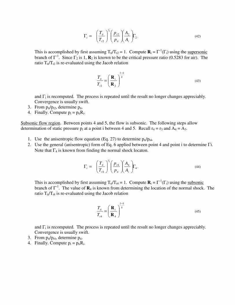
Supersonic flow region. Between points 2 and 3 the flow is supersonic. The following steps are used to

determine the static pressure pi at a point between 2 and 3:

1. Use the anisentropic flow equation (Eq. 27) to determine pti/pt2.

2. Use the general (anisentropic) form of Eq. 6 applied between point 2 and point i, and the fact that

Γ2 = 1, to determine Γi:

2

22

2

21

Γ

=Γ

iti

t

t

ti

iA

A

p

p

T

T. (42)

This is accomplished by first assuming Tti/Tt2 = 1. Compute Ri = Γ-1(Γi) using the supersonic

branch of Γ-1. Since Γ2 is 1, R2 is known to be the critical pressure ratio (0.5283 for air). The

ratio Tti/Tt2 is re-evaluated using the Jacob relation

k

k

i

t

ti

T

T−

=

1

22 R

R (43)

and Γi is recomputed. The process is repeated until the result no longer changes appreciably.

Convergence is usually swift.

3. From pti/pt2, determine pti.

4. Finally. Compute pi = ptiRi.

Subsonic flow region. Between points 4 and 5, the flow is subsonic. The following steps allow

determination of static pressure pi at a point i between 4 and 5. Recall r4 = r3 and A4 = A3.

1. Use the anisentropic flow equation (Eq. 27) to determine pti/pt4.

2. Use the general (anisentropic) form of Eq. 6 applied between point 4 and point i to determine Γi.

Note that Γ4 is known from finding the normal shock locaton.

4

44

4

21

Γ

=Γ

iti

t

t

ti

iA

A

p

p

T

T. (44)

This is accomplished by first assuming Tti/Tt4 = 1. Compute Ri = Γ-1(Γi) using the subsonic

branch of Γ-1. The value of R4 is known from determining the location of the normal shock. The

ratio Tti/Tt4 is re-evaluated using the Jacob relation

k

k

i

t

ti

T

T−

=

1

44 R

R (45)

and Γi is recomputed. The process is repeated until the result no longer changes appreciably.

Convergence is usually swift.

3. From pti/pt4, determine pti.

4. Finally. Compute pi = ptiRi.

Appendices

Appendix 1: General Solution to the Isothermal Flow Equation and Derivation of the Jacob Relation

The General Gas Dynamics Equation is

21

2

1

2

1

21

1

2 Γ=Γ

A

A

p

p

T

T

t

t

t

t. (46)

In [2] the author applies this equation to cases of anisentropic, isothermal flow, but restricts himself to

considering only cases where A1 = A2, i.e. constant-area flow, claiming that the general case does not

admit closed solutions. Engineers, however, know that closed solutions are not always necessary to

obtain numerical results.

Assume pt1/pt2 is known for some anisentropic flow. Also assume Γ1 and the ratio A1/A2 are known. To

determine Γ2 it is necessary to make one additional assumption. It will be seen that the isothermal

assumption is the most natural to make, is reasonable in practice, and leads immediately to a solution.

Begin by assuming (incorrectly) that Tt2/Tt1 = 1. Compute Γ2. Determine R2 from the inverse of Γ2,

consistently using whichever branch of the Γ-1 function applies.

The total temperature and total pressure of a point in the flow are related by the polytrope

k

k

tt

p

p

T

T1−

= . (47)

Substituting the pressure ratio R2 = p2/pt2 and dividing state 2 by state 1, one may write

( )

( ) k

k

k

k

t

t

T

T

T

T

−

−

=1

1

1

2

1

1

2

2

R

R. (48)

or, rearranging,

k

k

t

t

T

T

T

T−

=

1

1

2

2

1

1

2

R

R. (49)

The goal is to find an expression for Tt2/Tt1, which was initially assumed unity. Unless T1/T2 is known a

priori, it is easiest to adopt the isothermal assumption and take T1/T2 = 1. Since the very narrow passage

of a bearing clearance certainly provides ample opportunity for heat exchange, this is not an

unreasonable assumption in this particular application. Doing so results in the Jacob relation

k

k

t

t

T

T−

=

1

1

2

1

2

R

R. (50)

Using this value of Tt2/Tt1, Γ2 and R2 are recomputed, and the process repeated until changes in the

value of Γ2 are below the required level of accuracy. Convergence to a high degree of accuracy is

usually obtained in just a few iterations. Since this clever solution is not found in any of the books I’ve

seen, I’ve decided to name it after myself.

Appendix 2: Bearing Inlet Recesses, Orifice Shocks and Critical Clearance Entry

It may be desirable to compute the total pressure reduction encountered across an orifice restriction

rather than to assume a constant orifice loss coefficient. It may also be simply instructive to understand

orifice flow and the physical origin of the total pressure reduction.

If the orifice opens into a recess in the bearing, a shock may form around the orifice outlet (see Fig. 4).

Even though the Mach number is never greater than one in the throat, it may accelerate to supersonic

speeds as it enters the recess. The reason it can do so relates to way the normal area changes. A

geometrically perfectly abrupt change in area is experienced by the flow as a more gradual change. The

area normal to the flow resembles a hemisphere surrounding the orifice outlet, since the flow cannot

expand instantaneously as it exits. The flow expands in a bullet-shaped pattern beyond the orifice,

capped by a normal shock as the gas decelerates to conditions within the recess. If the flow is increased

even more, the shock occupies an increasing portion of the recess.

Figure 4. Bearing inlet with recess.

D

d

flow

shock

The utility of providing recesses is apparent if it causes supersonic flows to be restricted to a very

limited region around the inlet. At a properly selected supply pressure, the normal shock will be trapped

by the recess and not move into the clearance, where it would erode the load-carrying capacity of the

bearing.

The following analysis determines the minimum recess diameter D and depth d for shock containment at

a given operating clearance. Refer to Fig. 4.

Given a mass flow rate w at the throat (found e.g. using Eq. 33) and a minimum operating clearance h,

the minimum required recess diameter to prevent supersonic flow from recurring upon entry into the

clearance is found as follows. At the point of entry into the clearance, the normal area is πDh. Assume

a shock has occurred in the recess, and flow is now subsonic. For flow to remain subsonic as it

accelerates and enters the clearance, M must be less than unity at that point.

It is useful to introduce the total flow number,

( )12

1

2

2

11

−

+

−+

==k

kt

t k

kRT

Ap

w

M

Mα . (51)

The critical flow number, α*, is the flow number at Mach 1. For air (k = 1.4), α* is approximately

0.6847. Since we wish the Mach number to remain less than unity through this point, we require the

state point flow number to be less than the critical flow number. This leads to the inequality

*α<t

t

RTAp

w. (52)

Substituting the expression for clearance entry area and solving, one finds

t

t

RTph

wD

*απ> . (53)

This minimum diameter ensures a large enough entry area to prevent acceleration of a subsonic fluid to

Mach 1. Since the normal area is smallest at the clearance entry and increases linearly into the

clearance, a subsonic flow through the entry remains subsonic throughout the clearance. Thus, the

highest static pressure, and by extension the highest load capacity, is obtained.

To be sure that a normal shock does occur in the recess and that fluid entering the clearance is subsonic,

one must select the appropriate recess depth. To do this, assume a depth d, such that the normal area

prior to clearance entry is πD(d+h). Assume this as the initial area and complete one iteration of the

steps for finding a normal shock location (see section 4), assuming isentropic flow in the recess

upstream of the shock. If the area obtained in step 11 is much less than the area assumed, then the shock

will occur at a point inside the recess.

Υ

If a value for the area is found which is very close to the initial value, care must be taken. When a large

step is encountered, the fluid will begin to accelerate well before the step is passed. Therefore, do not

assume a normal shock within a distance d of the step will actually occur. Increase the initial recess

depth d slightly and try again.

A warning about recesses in compressible-fluid bearings: Significant recess volumes

can act as mass storage devices, and can phase-delay changes in static pressure which

normally stabilize the bearing. When such changes are significant, the gas supply can

begin driving oscillations in the bearing at the rotor-bearing natural frequency, otherwise known as

pneumatic instability or air hammer (6). Therefore all due care should be taken to keep recess volumes

to a minimum.

References

1. Vohr, J. H., "A Study of Inherent Restriction Characteristics for Hydrostatic Gas Bearings," Vol.2,

Paper 30, Proceedings of Fourth Gas Bearing Symposium, April 1969, University of Southampton.

2. Benedict, R. P., “Fundamentals of Gas Dynamics,” John Wiley & Sons, 1983.

3. Fox, R. W. and A. T. McDonald, “Introduction to Fluid Mechanics,” 4th

ed., John Wiley & Sons,

Inc., New York, 1992, p. 778.

4. Fuller, D. D., “Theory and Practice of Lubrication for Engineers,” John Wiley & Sons, New York,

1984, p. 490 ff.

5. Licht, L. and D. D. Fuller, "A Preliminary Investigation of an Air-Lubricated Hydrostatic Thrust

Bearing," Paper No. 54-Lub-18, Am. Soc. Mech. Engrs., 1954.

6. Jacob, J.S., J.J. Yu, D.E. Bently, P. Goldman, 2001, “Air-hammer instability of externally-

pressurized compressible-fluid bearings,” Proc. ISCORMA-1, 20-24 Aug, So. Lake Tahoe, CA,

USA, paper 2015.