Supervised Hierarchical Pitman-Yor Process for Natural Scene Segmentation

Alex ShyrUC Berkeley

Trevor DarrellICSI, UC Berkeley

Michael JordanUC Berkeley

Raquel UrtasunTTI Chicago

Abstract

From conventional wisdom and empirical studies of an-notated data, it has been shown that visual statistics suchas object frequencies and segment sizes follow power lawdistributions. Using these two as prior distributions, thehierarchical Pitman-Yor process has been proposed for thescene segmentation task. In this paper, we add label in-formation into the previously unsupervised model. Our ap-proach exploits the labelled data by adding constraints onthe parameter space during the variational learning phase.We evaluate our formulation on the LabelMe natural scenedataset, and show the effectiveness of our approach.

1. IntroductionThe problem of image segmentation and grouping re-

mains one of the important challenges in computer vision,as segmenting a scene into semantic categories is one of thekey steps towards scene understanding. As evidenced bythe PASCAL VOC challenge [7], segmentation is still anunsolved problem - the accuracy of existing approaches isstill insufficient for integration into real-world applications,e.g., robotics.

In the past few years, approaches based on Markov ran-dom fields (MRF) have been popular for segmentation [13][11] [15]. In these approaches, the image is modelled as anundirected graphical model, with nodes being pixels and/orsuperpixels. Node potentials are defined in terms of thelocal evidence, and edge potentials are defined to encour-age smoothness in the segmentation. The resulting infer-ence problem is either solved by graph-cuts [4] or message-passing algorithms [9].

While very effective for certain tasks, these probabilis-tic models do not reflect the underlying statistics of natu-ral images. Recent studies show that a wide range of natu-ral image statistics are distributed according to heavy-taileddistributions. This problem has been noticed not only forsegmentation, but also for optical flow (denoising) [25], in-trinsic images [33] and layer extraction [1]. Moreover, longrange dependencies are difficult to capture with MRFs.

The gPb method of [17] computes long-range interac-

tions by building an affinity matrix from local cues viathe Pb response[18] and computing gradients of the corre-sponding eigenvectors. These gradients are then combinedwith local feature gradients to obtain the final gPb function.[2] applies the oriented watershed transform (OWT) of thegPb response to form regions, and subsequently constructthe ultrametric contour map (UCM), defining a hierarchi-cal segmentation. We adopt the gPb function as a basicboundary model, and we demonstrate in our experimentsthat a probabilistic model with a prior which succinctly de-scribes segment statistics achieves better performance thanthe OWT-UCM model.

Sudderth and Jordan [30] proposed an unsupervisedprobabilistic model for segmentation that is based on theHierarchical Pitman-Yor process (HPY), which is a non-parametric Bayesian prior over infinite partitions. The HPYprocess is a generalization of the hierarchical Dirichlet pro-cesses (HDP), with heavier-tailed power law prior distribu-tions. Confirming the findings of Sudderth et al., we showthat the distribution over the size of natural segments as wellas the frequencies that objects appear in an image follow apower law distribution. Long range dependencies are in-troduced in their framework via thresholded Gaussian pro-cesses. Their approach, however, is unsupervised, and doesnot leverage the ever growing abundance of annotations andground truth data, e.g., LabelMe. As a consequence, the in-ferred segmentations are not always accurate and have roomfor improvement.

In this paper we propose a novel supervised discrimina-tive Hierarchical Pitman-Yor process (DHPY) approach tosegmentation. In particular, we frame the learning as a reg-ularized constrained optimization problem, where we max-imize a variational lower bound on the log likelihood whileimposing the inferred labels at the segment and object lev-els agree with the ground truth annotations. We borrow in-tuitions from the literature of cutting plane and subgradi-ent optimization methods, and derive an efficient methodto train the HPY. At every step of the algorithm the mostviolated constraint is introduced into the optimization viaLagrange multipliers. While we leverage the additional an-notations, we also inherit the nice properties of [30]; morespecifically, we are able to capture long range dependencies

2281

via thresholded Gaussian process, and we retain the naturalpower-law priors.

We demonstrate the effectiveness of our approach in adataset composed of 8 different types of scenes and 100 ob-ject categories taken from the LabelMe dataset [26]. Ourapproach outperforms normalized cuts [28], the UltrametricContour Map approach of [2], as well as the unsupervisedHPY [30]. In the remainder of the paper we first review therelated work. We then introduce the HPY process, deriveour supervised DHPY formulation, show empirical results,and conclude with avenues of future research.

2. Related WorkMarkov Random Fields (MRFs) have become a popu-

lar approach to segmentation, as demonstrated by the largebody of work [13, 11, 15]. In these approaches the imageis modeled as an undirected graphical model at the levelof pixels and/or superpixels. Node potentials describe lo-cal evidence and edge potentials usually encourage smooth-ness for neighboring pixels/superpixels with the same label.Several approaches to inference have been proposed for theMRF, such as graph cuts [4] and belief propagation [9].

One particular form of MRF that directly defines a dis-criminative distribution of the latent states is the Condi-tional Random Field (CRF) [29]. Inference is made eas-ier since the conditional probabilities of the latent labelsgiven the observations are modelled directly. Anotherway that supervision is used is through the fusing of con-textual information [15]. Context can be added in theform of global constraints which usually specify class-co-occurrence and/or conditional dependence in the form ofclique structure.

While effective for segmentation, MRFs have beenshown to be inadequate for modelling the visual statisticsof natural scenes [27]. In this paper, we build on top of theHierarchical Pitman-Yor processes, which accurately modelthe power law prior distributions, such as the distributionsover the number of objects per image as well as that of thesize of natural segments.

Recently, [5, 6] show that segmentation can be framedas a two step process. First, candidate segments which canbe part of an object are identified - [5] employs a graph-cutoptimization framework, while [6] uses a CRF model. Thesegmentation problem is then formulated as a ranking prob-lem over the candidate segments, which involves computingsegment-level features such as segment area, perimeter andshape statistics.

Sudderth and Jordan [30] proposed an unsupervised ap-proach to image segmentation that models segments of vi-sual scenes with a hierarchical Pitman-Yor process (HPY).Thresholded Gaussian process are utilized to capture spatialcoherence among regions. Moreover, this captures long-range dependences among the observations, which are diffi-

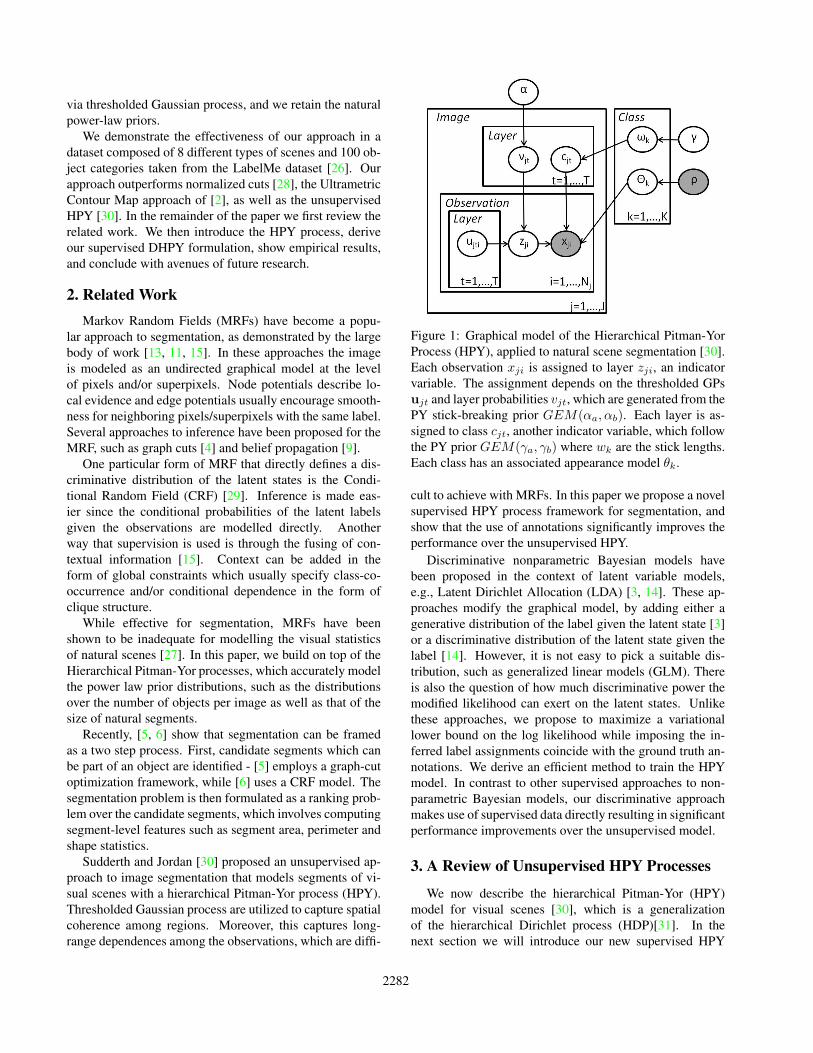
Figure 1: Graphical model of the Hierarchical Pitman-YorProcess (HPY), applied to natural scene segmentation [30].Each observation xji is assigned to layer zji, an indicatorvariable. The assignment depends on the thresholded GPsujt and layer probabilities vjt, which are generated from thePY stick-breaking prior GEM(αa, αb). Each layer is as-signed to class cjt, another indicator variable, which followthe PY prior GEM(γa, γb) where wk are the stick lengths.Each class has an associated appearance model θk.

cult to achieve with MRFs. In this paper we propose a novelsupervised HPY process framework for segmentation, andshow that the use of annotations significantly improves theperformance over the unsupervised HPY.

Discriminative nonparametric Bayesian models havebeen proposed in the context of latent variable models,e.g., Latent Dirichlet Allocation (LDA) [3, 14]. These ap-proaches modify the graphical model, by adding either agenerative distribution of the label given the latent state [3]or a discriminative distribution of the latent state given thelabel [14]. However, it is not easy to pick a suitable dis-tribution, such as generalized linear models (GLM). Thereis also the question of how much discriminative power themodified likelihood can exert on the latent states. Unlikethese approaches, we propose to maximize a variationallower bound on the log likelihood while imposing the in-ferred label assignments coincide with the ground truth an-notations. We derive an efficient method to train the HPYmodel. In contrast to other supervised approaches to non-parametric Bayesian models, our discriminative approachmakes use of supervised data directly resulting in significantperformance improvements over the unsupervised model.

3. A Review of Unsupervised HPY Processes

We now describe the hierarchical Pitman-Yor (HPY)model for visual scenes [30], which is a generalizationof the hierarchical Dirichlet process (HDP)[31]. In thenext section we will introduce our new supervised HPY

2282

model. The Pitman-Yor process [22], denoted by φ ∼GEM(γa, γb), places a prior distribution over partitionswith hyperparameters γa, γb satisfying 0 ≤ γa < 1 andγb > −γa. It can be defined using the stick-breaking con-struction as

φk = wk

k−1∏l=1

(1− wl) = wk(1−k−1∑l=1

φl), with

wk ∼ Beta(1− γa, γb + kγa). (1)

The {φk} are the partition probabilities, while the {wk}are the stick lengths. Note that we recover a Dirichlet pro-cess, specified by a single concentration parameter γb, whenγa = 0. When γa > 0, the partition probabilities followa power-law distribution with a heavy tail. While the PYprocess is a prior on infinite partitions, only a finite subsetof partitions will have positive probabilities greater than athreshold ε. Hence, the PY process implicitly imposes aprior on the number of partitions.

In the HPY model, two Pitman-Yor process priors areplaced over the distributions of global class categories andsegment proportions. Fig. 1 shows the directed graphicalmodel. Each image is segmented into superpixels, whichare from now on treated as the observed data units xji. Eachdata point is then assigned to a layer with probability

P [zji = t|zji 6= t−1, . . . , 1] = P [ujti < Φ−1(vjt)] = vjt,

where we have introduced a zero mean Gaussian process(GP) ujt for each layer t. These thresholded GPs com-pletely determine the layer assignment of each superpixel,with the assignment rule being

zji = min{t|ujti < Φ−1(vjt)}. (2)

Each layer is associated with a global object class cjtwith an appearance model θk. The emission probability isthen

p(xji|zji = t, cjt = k,θ) = Mult(xji|θk). (3)

with θ = {θ1, · · · } To place PY priors on the dis-tributions over global class categories and segment pro-portions, the class assignments cjt are sampled fromφ ∼ GEM(γa, γb), which is the stick-breaking prior de-scribed above, with wk the stick length. Similarly, thelayer assignment probabilities vjt are sampled from π ∼GEM(αa, αb).

4. Supervised Hierarchical Pitman-Yor ModelIn this section we present our supervised hierarchical

Pitman-Yor process model for image segmentation. We firstderive our variational learning approach and show how toincorporate supervision by solving a constrained optimiza-tion problem. We then derive a cutting plane method toefficiently learn the model.

Following [30], we train the HPY model with a meanfield variational approximation. A completely factorizedvariational posterior is introduced as follows

q(u,v, c,w,θ) =

K∏k=1

q(wk|ωk)q(θk|ηk)×

×J∏j=1

T∏t=1

q(vjt|νjt)q(cjt|κjt)Nj∏i=1

q(ujti|µjti),

where the distributions are, with v̄jt = Φ−1(vjt),

q(θk|ηk) = Dir(ηk)

q(cj |κj) = Mult(cj |κj)q(wk|ωk,a, ωk,b) = Beta(wk|ωk,a, ωk,b)q(v̄jt|νjt, δjt) = N(v̄jt|νjt, δjt)

q(ujti|µjti, λjti) = N(ujti|µjti, λjti).

We truncate the variational posterior by setting q(vjT =1) = 1 and q(wK = 1) = 1. We then train the model byoptimizing the lower bound on the marginal likelihood

log p(x|α, γ, ρ) ≥ H(q) + Eq[log p(x, z,u,v, c,w, θ|α, γ, ρ)]

= Eq[log p(x, z,u,v, c,w, θ|α, γ, ρ)]− Eq[log q(u,v, c,w, θ)] ≡ L

This is equivalent to minimizing the KL-divergence be-tween p and q. The optimization is done through a com-bination of closed-form updates and gradient descent.

Inference in the unsupervised HPY model produce layer-level and class-level segmentations using the variationalmarginals arg maxt Pq(zji = t) and arg maxk Pq(cjt =k), where

Pq(zji = t) = Φ(νjt − µjti√δjt + λjti

)

t−1∏τ=1

(1− Φ(νjτ − µjτi√δjτ + λjτi

))

Pq(cjt = k) = κjtk

= exp{∑i,l

xji,lPq(zji = t)Eq log ηk,l +

k∑k′=1

Eq logωk′,l},

with Eq log ηk,l = Ψ(ηk,l) − Ψ(∑l ηk,l) and Eq logωk′,l

= Ψ(ωk′,t)−Ψ(ωk′,t + ωk′,b) from the Dirichlet posteriorassumption. The last equation stems from the closed-formupdate for κjtk.

Let A be the set of annotations. We are provided withtwo types of annotations:

A ={

(asji, acji)|asji ∈ {1, . . . , T}, acji ∈ {1, . . . ,K}

}where asji : segment-level annotation, and

acji : class-level annotation.

Segment-level annotations describe the layer assignment ofeach observation, while class-level annotation describes theclass assignment of each layer. Note that we have imposedan absolute ordering on the layers, due to the stick-breaking

2283

construction of the layer model; in practice, we sort the dif-ferent layers in decreasing order of their sizes.

We apply supervision constrains that are added to thevariational program. Learning the supervised HPY can thenbe formulated as the following maximization problem

max Ls.t. ∀(j, i) ∈ A, Pq(zji = asji) ≥ max

tPq(zji = t)

∀(j, i) ∈ A, Pq(cjasji = acji) ≥ maxk

Pq(cjasji = k)

with respect to µjti, λjti, νjt and δjt. Note that the aboveprobabilities have been defined perviously in terms of thesevariables.

We transform the above optimization problem into a sin-gle objective by adding slack variables

max L −∑

(i,j)∈A(Csζsji + Ccζcji)

s.t. ∀(j, i) ∈ A, Pq(zji = asji) + ζsji ≥ maxt Pq(zji = t)

∀(j, i) ∈ A, Pq(cjasji = acji) + ζcji ≥ maxk Pq(cjasji = k)

The Lagrangian ` can then be defined as

` = L − Cs∑

(i,j)∈A

(maxtPq(zji = t)− Pq(zji = asji))

−Cc∑

(i,j)∈A

(maxk

Pq(cjasji = k)− Pq(cjasji = acji))

Maximizing the Lagrangian defines the optimization prob-lem we solve to learn the discriminative HPY model. Thecoefficients Cs and Cc determine the relative weighting themodel puts on minimizing the KL divergence and minimiz-ing the segmentation error.

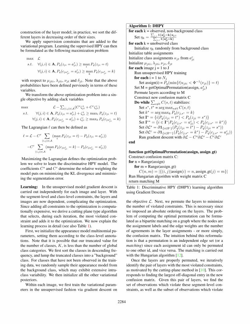
Learning: In the unsupervised model gradient descent iscarried out independently for each image and layer. Withthe segment-level and class-level constraints, the layers andimages are now dependent, complicating the optimization.Since adding all constraints to the optimization is computa-tionally expensive, we derive a cutting plane type algorithmthat selects, during each iteration, the most violated con-straint and adds it to the optimization. We now explain thelearning process in detail (see also Table 1).

First, we initialize the appearance model multinomial pa-rameters, setting them according to the class-level annota-tions. Note that it is possible that our truncated value forthe number of classes, K, is less than the number of globalclass categories. We first sort the classes in descending fre-quency, and lump the truncated classes into a ”background”class. For classes that have not been observed in the train-ing data, we randomly sample their appearance model fromthe background class, which may exhibit extensive intra-class variability. We then initialize all the other variationalposteriors.

Within each image, we first train the variational param-eters in the unsupervised fashion via gradient descent on

Algorithm 1: DHPYfor each k = observed, non-background class

Set ηk =∑

j,i 1{acji=k}xj,i∑

j,i 1{acji=k}

for each k = unobserved classInitialize ηk randomly from background class

Initialize table assignmentsInitialize class assignments κjt from acjiInitialize µjti, λjti, νjt, δjtfor each image j = 1 to J

Run unsupervised HPY trainingfor each i = 1 to Nj

Set assign(i) = Pq(min{t|ujti < Φ−1(vjt)} = t)Set M = getOptimalPermutation(assign, asji)Permute layers according to MConstruct new confusion matrix CDo while

∑s6=t C(s, t) stabilizes:

Set s∗, t∗ = arg maxs 6=t C(s, t)Set k∗ = arg maxk Pq(cj,s∗ = k)Set I∗ = {i|Pq(zji = t∗) < Pq(zji = s∗)}Set I∗∗ = {i ∈ I∗|Pq(cj,s∗ = acji) < Pq(cj,s∗ = k∗)}Set ∂Ls = ∂1{i∈I∗}(Pq(zji = t∗)− Pq(zji = s∗))Set ∂Lc = ∂1{i∈I∗∗}(Pq(cj,s∗ = k∗)− Pq(cj,s∗ = acji))Run gradient descent with ∂L − Cs∂Ls − Cc∂Lc

end

function getOptimalPermutation(assign, assign gt)Construct confusion matrix C:for n = Range(assign)

for m = Range(assign gt)C(n,m) = |{(i, j)|assign(i) = n, assign gt(j) = m}|

Run Hungarian algorithm with weight matrix Creturn matching M

Table 1: Discriminative HPY (DHPY) learning algorithmusing Gradient Descent

the objective L. Next, we permute the layers to minimizethe number of violated constraints. This is necessary sincewe imposed an absolute ordering on the layers. The prob-lem of computing the optimal permutation can be formu-lated as a bipartite matching on a graph where the nodes arethe assignment labels and the edge weights are the numberof agreements in the layer assignments - or more simply,the confusion matrix. The intuition behind this reformula-tion is that a permutation is an independent edge set (or amatching) since each assignment id can only be permutedto one other id, and vice versa. The matching is carried outwith the Hungarian algorithm [12].

Once the layers are properly permuted, we iterativelyidentify the pair of layers with the most violated constraints,as motivated by the cutting-plane method in [10]. This cor-responds to finding the largest off-diagonal entry in the newconfusion matrix. Given this pair of layers, we find theset of observations which violate these segment-level con-straints, as well as the subset of observations which violate

2284

100 101 102 103 10410 5

10 4

10 3

10 2

10 1Log log plot of Segment Size Distribution

Segment Sizes

Den

sity

PY(0.65, 4.8)EmpiricalDistribution

100 101 102 103 10410 4

10 3

10 2

10 1

100Log log plot of Class Distribution

Class Counts

Den

sity

PY(0.7, 0.5)EmpiricalDistribution

0 50 100 150 2000

0.1

0.2

0.3

0.4

0.5

0.6

0.7

0.8

0.9

1

Number of Training Examples

Rand

Inde

x

Average over all categories

N CutOWT UCMHPYDHPY

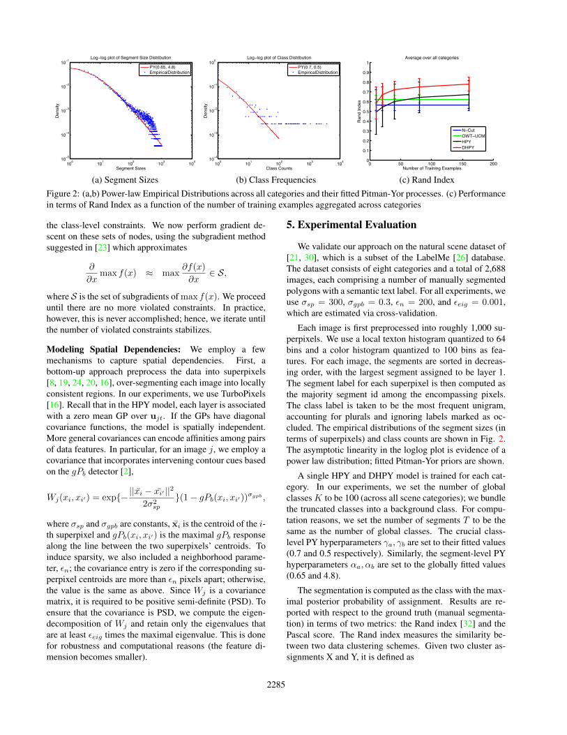
(a) Segment Sizes (b) Class Frequencies (c) Rand IndexFigure 2: (a,b) Power-law Empirical Distributions across all categories and their fitted Pitman-Yor processes. (c) Performancein terms of Rand Index as a function of the number of training examples aggregated across categories

the class-level constraints. We now perform gradient de-scent on these sets of nodes, using the subgradient methodsuggested in [23] which approximates

∂

∂xmax f(x) ≈ max

∂f(x)

∂x∈ S,

where S is the set of subgradients of max f(x). We proceeduntil there are no more violated constraints. In practice,however, this is never accomplished; hence, we iterate untilthe number of violated constraints stabilizes.

Modeling Spatial Dependencies: We employ a fewmechanisms to capture spatial dependencies. First, abottom-up approach preprocess the data into superpixels[8, 19, 24, 20, 16], over-segmenting each image into locallyconsistent regions. In our experiments, we use TurboPixels[16]. Recall that in the HPY model, each layer is associatedwith a zero mean GP over ujt. If the GPs have diagonalcovariance functions, the model is spatially independent.More general covariances can encode affinities among pairsof data features. In particular, for an image j, we employ acovariance that incorporates intervening contour cues basedon the gPb detector [2],

Wj(xi, xi′) = exp{−||x̄i − x̄i′ ||2

2σ2sp

}(1− gPb(xi, xi′))σgpb ,

where σsp and σgpb are constants, x̄i is the centroid of the i-th superpixel and gPb(xi, xi′) is the maximal gPb responsealong the line between the two superpixels’ centroids. Toinduce sparsity, we also included a neighborhood parame-ter, εn; the covariance entry is zero if the corresponding su-perpixel centroids are more than εn pixels apart; otherwise,the value is the same as above. Since Wj is a covariancematrix, it is required to be positive semi-definite (PSD). Toensure that the covariance is PSD, we compute the eigen-decomposition of Wj and retain only the eigenvalues thatare at least εeig times the maximal eigenvalue. This is donefor robustness and computational reasons (the feature di-mension becomes smaller).

5. Experimental Evaluation

We validate our approach on the natural scene dataset of[21, 30], which is a subset of the LabelMe [26] database.The dataset consists of eight categories and a total of 2,688images, each comprising a number of manually segmentedpolygons with a semantic text label. For all experiments, weuse σsp = 300, σgpb = 0.3, εn = 200, and εeig = 0.001,which are estimated via cross-validation.

Each image is first preprocessed into roughly 1,000 su-perpixels. We use a local texton histogram quantized to 64bins and a color histogram quantized to 100 bins as fea-tures. For each image, the segments are sorted in decreas-ing order, with the largest segment assigned to be layer 1.The segment label for each superpixel is then computed asthe majority segment id among the encompassing pixels.The class label is taken to be the most frequent unigram,accounting for plurals and ignoring labels marked as oc-cluded. The empirical distributions of the segment sizes (interms of superpixels) and class counts are shown in Fig. 2.The asymptotic linearity in the loglog plot is evidence of apower law distribution; fitted Pitman-Yor priors are shown.

A single HPY and DHPY model is trained for each cat-egory. In our experiments, we set the number of globalclassesK to be 100 (across all scene categories); we bundlethe truncated classes into a background class. For compu-tation reasons, we set the number of segments T to be thesame as the number of global classes. The crucial class-level PY hyperparameters γa, γb are set to their fitted values(0.7 and 0.5 respectively). Similarly, the segment-level PYhyperparameters αa, αb are set to the globally fitted values(0.65 and 4.8).

The segmentation is computed as the class with the max-imal posterior probability of assignment. Results are re-ported with respect to the ground truth (manual segmenta-tion) in terms of two metrics: the Rand index [32] and thePascal score. The Rand index measures the similarity be-tween two data clustering schemes. Given two cluster as-signments X and Y, it is defined as

2285

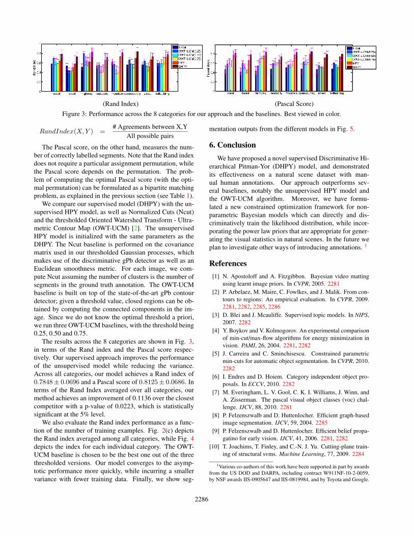
(Rand Index) (Pascal Score)Figure 3: Performance across the 8 categories for our approach and the baselines. Best viewed in color.

RandIndex(X,Y ) =# Agreements between X,Y

All possible pairs

The Pascal score, on the other hand, measures the num-ber of correctly labelled segments. Note that the Rand indexdoes not require a particular assignment permutation, whilethe Pascal score depends on the permutation. The prob-lem of computing the optimal Pascal score (with the opti-mal permutation) can be formulated as a bipartite matchingproblem, as explained in the previous section (see Table 1).

We compare our supervised model (DHPY) with the un-supervised HPY model, as well as Normalized Cuts (Ncut)and the thresholded Oriented Watershed Transform - Ultra-metric Contour Map (OWT-UCM) [2]. The unsupervisedHPY model is initialized with the same parameters as theDHPY. The Ncut baseline is performed on the covariancematrix used in our thresholded Gaussian processes, whichmakes use of the discriminative gPb detector as well as anEuclidean smoothness metric. For each image, we com-pute Ncut assuming the number of clusters is the number ofsegments in the ground truth annotation. The OWT-UCMbaseline is built on top of the state-of-the-art gPb contourdetector; given a threshold value, closed regions can be ob-tained by computing the connected components in the im-age. Since we do not know the optimal threshold a priori,we run three OWT-UCM baselines, with the threshold being0.25, 0.50 and 0.75.

The results across the 8 categories are shown in Fig. 3,in terms of the Rand index and the Pascal score respec-tively. Our supervised approach improves the performanceof the unsupervised model while reducing the variance.Across all categories, our model achieves a Rand index of0.7848± 0.0696 and a Pascal score of 0.8125± 0.0686. Interms of the Rand Index averaged over all categories, ourmethod achieves an improvement of 0.1136 over the closestcompetitor with a p-value of 0.0223, which is statisticallysignificant at the 5% level.

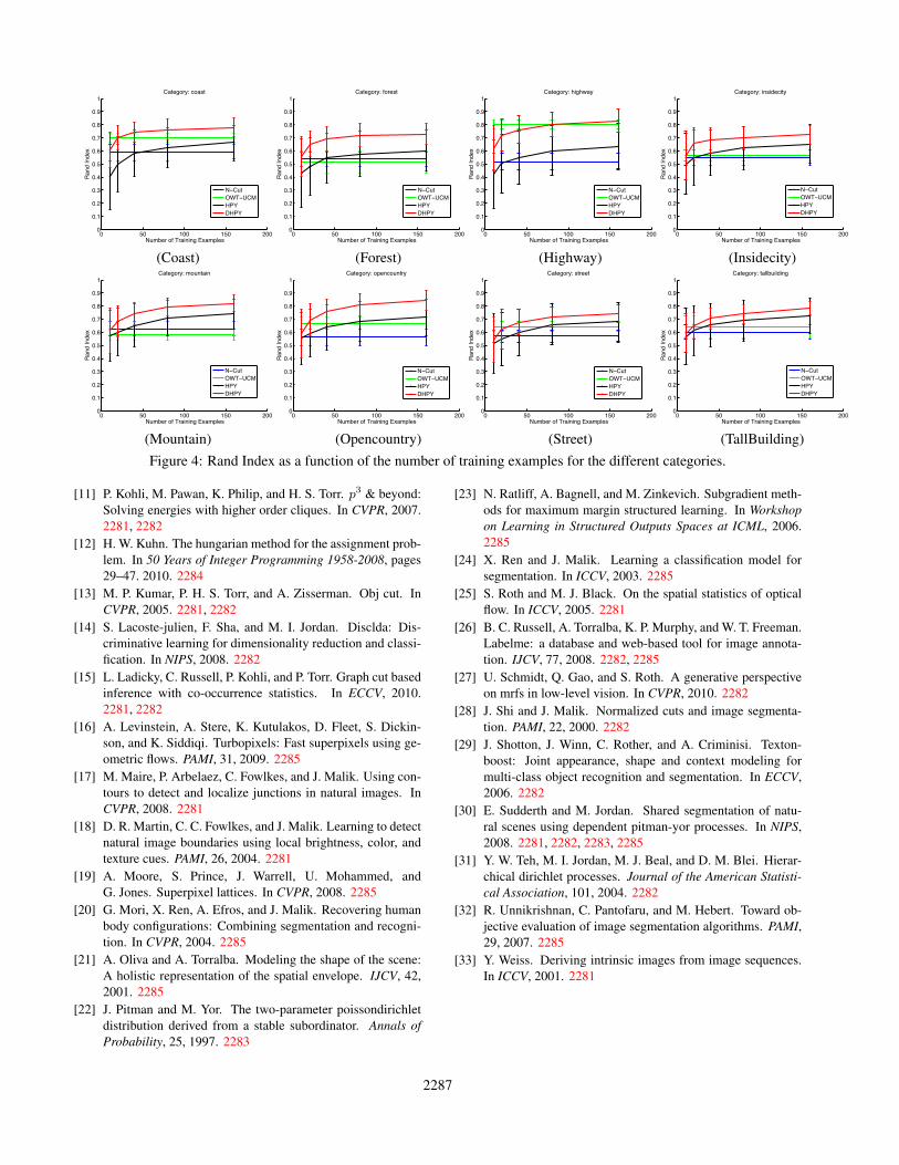
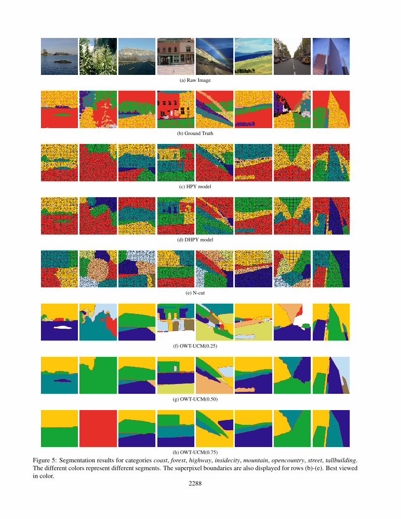
We also evaluate the Rand index performance as a func-tion of the number of training examples. Fig. 2(c) depictsthe Rand index averaged among all categories, while Fig. 4depicts the index for each individual category. The OWT-UCM baseline is chosen to be the best one out of the threethresholded versions. Our model converges to the asymp-totic performance more quickly, while incurring a smallervariance with fewer training data. Finally, we show seg-

mentation outputs from the different models in Fig. 5.

6. ConclusionWe have proposed a novel supervised Discriminative Hi-

erarchical Pitman-Yor (DHPY) model, and demonstratedits effectiveness on a natural scene dataset with man-ual human annotations. Our approach outperforms sev-eral baselines, notably the unsupervised HPY model andthe OWT-UCM algorithm. Moreover, we have formu-lated a new constrained optimization framework for non-parametric Bayesian models which can directly and dis-criminatively train the likelihood distribution, while incor-porating the power law priors that are appropriate for gener-ating the visual statistics in natural scenes. In the future weplan to investigate other ways of introducing annotations. 1

References[1] N. Apostoloff and A. Fitzgibbon. Bayesian video matting

using learnt image priors. In CVPR, 2005. 2281[2] P. Arbelaez, M. Maire, C. Fowlkes, and J. Malik. From con-

tours to regions: An empirical evaluation. In CVPR, 2009.2281, 2282, 2285, 2286

[3] D. Blei and J. Mcauliffe. Supervised topic models. In NIPS,2007. 2282

[4] Y. Boykov and V. Kolmogorov. An experimental comparisonof min-cut/max-flow algorithms for energy minimization invision. PAMI, 26, 2004. 2281, 2282

[5] J. Carreira and C. Sminchisescu. Constrained parametricmin-cuts for automatic object segmentation. In CVPR, 2010.2282

[6] I. Endres and D. Hoiem. Category independent object pro-posals. In ECCV, 2010. 2282

[7] M. Everingham, L. V. Gool, C. K. I. Williams, J. Winn, andA. Zisserman. The pascal visual object classes (voc) chal-lenge. IJCV, 88, 2010. 2281

[8] P. Felzenszwalb and D. Huttenlocher. Efficient graph-basedimage segmentation. IJCV, 59, 2004. 2285

[9] P. Felzenszwalb and D. Huttenlocher. Efficient belief propa-gatino for early vision. IJCV, 41, 2006. 2281, 2282

[10] T. Joachims, T. Finley, and C.-N. J. Yu. Cutting-plane train-ing of structural svms. Machine Learning, 77, 2009. 2284

1Various co-authors of this work have been supported in part by awardsfrom the US DOD and DARPA, including contract W911NF-10-2-0059,by NSF awards IIS-0905647 and IIS-0819984, and by Toyota and Google.

2286

0 50 100 150 2000

0.1

0.2

0.3

0.4

0.5

0.6

0.7

0.8

0.9

1Category: coast

Number of Training Examples

Rand

Inde

x

N CutOWT UCMHPYDHPY

0 50 100 150 2000

0.1

0.2

0.3

0.4

0.5

0.6

0.7

0.8

0.9

1Category: forest

Number of Training Examples

Rand

Inde

x

N CutOWT UCMHPYDHPY

0 50 100 150 2000

0.1

0.2

0.3

0.4

0.5

0.6

0.7

0.8

0.9

1Category: highway

Number of Training Examples

Rand

Inde

x

N CutOWT UCMHPYDHPY

0 50 100 150 2000

0.1

0.2

0.3

0.4

0.5

0.6

0.7

0.8

0.9

1Category: insidecity

Number of Training Examples

Rand

Inde

x

N CutOWT UCMHPYDHPY

(Coast) (Forest) (Highway) (Insidecity)

0 50 100 150 2000

0.1

0.2

0.3

0.4

0.5

0.6

0.7

0.8

0.9

1Category: mountain

Number of Training Examples

Rand

Inde

x

N CutOWT UCMHPYDHPY

0 50 100 150 2000

0.1

0.2

0.3

0.4

0.5

0.6

0.7

0.8

0.9

1Category: opencountry

Number of Training Examples

Rand

Inde

x

N CutOWT UCMHPYDHPY

0 50 100 150 2000

0.1

0.2

0.3

0.4

0.5

0.6

0.7

0.8

0.9

1Category: street

Number of Training Examples

Rand

Inde

x

N CutOWT UCMHPYDHPY

0 50 100 150 2000

0.1

0.2

0.3

0.4

0.5

0.6

0.7

0.8

0.9

1Category: tallbuilding

Number of Training Examples

Rand

Inde

x

N CutOWT UCMHPYDHPY

(Mountain) (Opencountry) (Street) (TallBuilding)Figure 4: Rand Index as a function of the number of training examples for the different categories.

[11] P. Kohli, M. Pawan, K. Philip, and H. S. Torr. p3 & beyond:Solving energies with higher order cliques. In CVPR, 2007.2281, 2282

[12] H. W. Kuhn. The hungarian method for the assignment prob-lem. In 50 Years of Integer Programming 1958-2008, pages29–47. 2010. 2284

[13] M. P. Kumar, P. H. S. Torr, and A. Zisserman. Obj cut. InCVPR, 2005. 2281, 2282

[14] S. Lacoste-julien, F. Sha, and M. I. Jordan. Disclda: Dis-criminative learning for dimensionality reduction and classi-fication. In NIPS, 2008. 2282

[15] L. Ladicky, C. Russell, P. Kohli, and P. Torr. Graph cut basedinference with co-occurrence statistics. In ECCV, 2010.2281, 2282

[16] A. Levinstein, A. Stere, K. Kutulakos, D. Fleet, S. Dickin-son, and K. Siddiqi. Turbopixels: Fast superpixels using ge-ometric flows. PAMI, 31, 2009. 2285

[17] M. Maire, P. Arbelaez, C. Fowlkes, and J. Malik. Using con-tours to detect and localize junctions in natural images. InCVPR, 2008. 2281

[18] D. R. Martin, C. C. Fowlkes, and J. Malik. Learning to detectnatural image boundaries using local brightness, color, andtexture cues. PAMI, 26, 2004. 2281

[19] A. Moore, S. Prince, J. Warrell, U. Mohammed, andG. Jones. Superpixel lattices. In CVPR, 2008. 2285

[20] G. Mori, X. Ren, A. Efros, and J. Malik. Recovering humanbody configurations: Combining segmentation and recogni-tion. In CVPR, 2004. 2285

[21] A. Oliva and A. Torralba. Modeling the shape of the scene:A holistic representation of the spatial envelope. IJCV, 42,2001. 2285

[22] J. Pitman and M. Yor. The two-parameter poissondirichletdistribution derived from a stable subordinator. Annals ofProbability, 25, 1997. 2283

[23] N. Ratliff, A. Bagnell, and M. Zinkevich. Subgradient meth-ods for maximum margin structured learning. In Workshopon Learning in Structured Outputs Spaces at ICML, 2006.2285

[24] X. Ren and J. Malik. Learning a classification model forsegmentation. In ICCV, 2003. 2285

[25] S. Roth and M. J. Black. On the spatial statistics of opticalflow. In ICCV, 2005. 2281

[26] B. C. Russell, A. Torralba, K. P. Murphy, and W. T. Freeman.Labelme: a database and web-based tool for image annota-tion. IJCV, 77, 2008. 2282, 2285

[27] U. Schmidt, Q. Gao, and S. Roth. A generative perspectiveon mrfs in low-level vision. In CVPR, 2010. 2282

[28] J. Shi and J. Malik. Normalized cuts and image segmenta-tion. PAMI, 22, 2000. 2282

[29] J. Shotton, J. Winn, C. Rother, and A. Criminisi. Texton-boost: Joint appearance, shape and context modeling formulti-class object recognition and segmentation. In ECCV,2006. 2282

[30] E. Sudderth and M. Jordan. Shared segmentation of natu-ral scenes using dependent pitman-yor processes. In NIPS,2008. 2281, 2282, 2283, 2285

[31] Y. W. Teh, M. I. Jordan, M. J. Beal, and D. M. Blei. Hierar-chical dirichlet processes. Journal of the American Statisti-cal Association, 101, 2004. 2282

[32] R. Unnikrishnan, C. Pantofaru, and M. Hebert. Toward ob-jective evaluation of image segmentation algorithms. PAMI,29, 2007. 2285

[33] Y. Weiss. Deriving intrinsic images from image sequences.In ICCV, 2001. 2281

2287

(a) Raw Image

(b) Ground Truth

(c) HPY model

(d) DHPY model

(e) N-cut

(f) OWT-UCM(0.25)

(g) OWT-UCM(0.50)

(h) OWT-UCM(0.75)

Figure 5: Segmentation results for categories coast, forest, highway, insidecity, mountain, opencountry, street, tallbuilding.The different colors represent different segments. The superpixel boundaries are also displayed for rows (b)-(e). Best viewedin color.

2288