supplementary information for: effects of structural
TRANSCRIPT
Supplementary Information for: Effects of Structural Change and Climate Policy on Long-Term Shifts in Lifecycle Energy Efficiency and Carbon Footprint
Authors: Sonia Yeh1, Gouri Shankar Mishra, Geoff Morrison, Jacob Teter Institute of Transportation Studies, University of California at Davis Raul Quiceno, Shell Research Limited Kenneth Gillingham, Yale School of Forestry & Environmental Studies Xavier Riera-Palou, Shell Research Limited Table of Contents: 1. Detailed Methodology
1.1 Calculation of Lifecycle Efficiency 1.2 General Assumptions 1.3 Primary to Secondary Conversion Assumptions and Post-hoc Calculations 1.4 Final to Useful Assumptions and Post-hoc Calculations
2. Decomposition Analysis 3. Scenario Results
3.1 Comparison of Results with Other Lifecycle Efficiency Estimates 3.2 Scenario Descriptions
3.3 Results by Resource (BAU scenario) 3.4 No Carbon Policy Scenarios
(BAU, Adv_EE_no_CCS, Adv_All_no_CCS) 3.5 RCP 6.0 Scenarios
(Ref_tech_no_CCS_RCP6.0, Ref_tech_CCS_RCP6.0, Adv_EE_no_CCS_RCP6.0, Adv_EE_CCS_RCP6.0, Adv_All_no_CCS_RCP6.0, Adv_All_CCS_RCP6.0)
3.6 RCP 4.5 Scenarios (Ref_tech_no_CCS_RCP4.5, Ref_tech_CCS_RCP4.5, Adv_EE_no_CCS_RCP4.5, Adv_EE_CCS_RCP4.5, Adv_All_noCCS_RCP4.5, Adv_All_CCS_RCP4.5)
3.7 Additional Figures Results comparing CCS Developed vs. Developing Countries
4. Global transportation primary energy use and energy pathway lifecycle carbon intensity 5. Exergy Efficiency: Assumptions and Results 6. References
1 Corresponding author, [email protected]

1. Detailed Methodology
1.1 Calculation of Lifecycle Energy Efficiency
Calculation of Lifecycle Energy Efficiency is a relatively straightforward accounting exercise which requires knowing the quantity of input and output energy of all energy conversions. For each end use and resource type, we multiply the series of conversion efficiencies between the primary and end use stages to estimate the pathway lifecycle energy efficiency for that end use. Table S1 provides three examples of how we calculate a pathway efficiency. Table S1. Example calculations of pathway efficiencies for Coal à Electricity à Industry; NG à Electricity à Building; and Crude à Transportation. The calculation begins with 1 EJ of primary energy on the left-hand side and demonstrates the subsequent energy conversions to arrive at useful energy (second column from right). Pathway efficiency is the useful energy divided by the primary energy. Primary EnergyàSecondaryàFinalàUseful
Primary Energy Secondary Final Useful Wep
ηps ηsf ηfu
Mined Coal àInput to
Coal Processing
àOutput from Coal Processing
àInput to Coal Electric
Plant
àOutput from Coal Electric
Plant
àInput to Manufact.
Plant
àUsed in Manufact.
Plant
Pathway Efficiency
1.00 EJ 1.00 EJ 0.99 EJ 0.89 0.28 EJ 0.25 EJ 0.18 EJ 18%
Unrefined Natural Gas
àInput to NG
Refinery
àOutput from NG Refinery
àInput to NG
Electric Plant
àOutput from NG Electric
Plant
àInput to Residential Buildings
àUsed in Residential
Building
Pathway Efficiency
1.00 EJ 0.95 EJ 0.92 EJ 0.87 EJ 0.29 EJ 0.26 EJ 0.24 EJ 24%
Conventional Raw Crude
àInput to Crude
Refinery
àOutput from Crude
Refinery
àDelivered Petroleum at
Service Station
àUsed in Light Duty Vehicles
Pathway Efficiency
1.0 EJ 0.98 EJ 0.91 EJ 0.91 EJ 0.12 EJ 12%
Once all pathway efficiencies of an energy resource are calculated, we estimate the resource’s lifecycle energy efficiency by summing the share-weighted pathways as shown in Table S2. Table S2. Examples of calculating the global economy-wide lifecycle energy efficiency of crude oil for selected years.
Energy pathway, ep 1995 2005 2010 Crude-->Industry Eff 0.59 0.58 0.61 Crude-->Transportation Eff 0.16 0.16 0.16 Crude-->Buildings Eff 0.76 0.82 0.83 Crude-->Electricity-->Buildings Eff 0.25 0.32 0.34 Crude-->Electricity-->Transportation Eff 0.14 0.14 0.13 Crude-->Electricity-->Industry Eff 0.18 0.18 0.19

Crude-->Industry Share 0.18 0.15 0.15 Crude-->Transportation Share 0.56 0.64 0.67 Crude-->Buildings Share 0.14 0.12 0.13 Crude-->Electricity-->Buildings Share 0.06 0.04 0.02 Crude-->Electricity-->Transportation Share 0.00 0.00 0.00 Crude-->Electricity-->Industry Share 0.06 0.04 0.02
Economy-wide Eff. 33% 31% 32% We repeat this exercise for each resource in each region and year. Similarly, regions are aggregated by summing the share-weighted efficiencies of each region. The aggregated global lifecycle efficiency is shown in the upper row of Fig. 3. We also aggregate regions into “developing” and “developed” later in the main text.
In places, GCAM lacks sufficient detail or is structured in a way that prohibits us from calculating the entire primary to useful efficiency of a given pathway. To overcome these deficiencies we make a number of assumptions or post-hoc calculations outlined below. Section 1.2 discusses general assumptions. Section 1.3 discusses assumptions and post-hoc calculations needed for the p→s conversion step while Section 1.4 discusses the f→u conversion step. 1.2 General Assumptions
1.2.1 Industrial Feedstocks: Globally, up to 25% of input energy to the industrial sector is incorporated into products such as plastics rather than burned as fuel. In calculating lifecycle energy efficiencies, we exclude these industrial feedstocks as done by Nakicenovic et al. (1) since no thermodynamic efficiency equivalent exists. Upon request, we can provide results with feedstocks by assuming a 100% efficiency in the base year and pegging the efficiency in subsequent years on the rate of change of material output/energy input in GCAM. Including industrial feedstocks increases the lifecycle energy efficiency of crude by up to 10% across scenarios, and increases coal, biomass, and natural gas lifecycle energy efficiencies by up to 3% across scenarios.
1.2.2 Allocation of Electricity: When electricity is created from an energy resource (e.g. coal), we assume it goes to a regional pool of electricity and is distributed to each end-user from that pool. As a result, our model does not link an electricity feedstock to a specific end-use. For example, for a given geographic region, the electricity used in manufacturing is assumed to be the same mix of electricity as used by electric vehicles. 1.2.3 Syngas and Biogas Allocation: Our calculations assume syngas from coal gasification and biogas from biomass gasification flow only to the industrial sector. This is consistent with GCAM modeling assumptions for these two energy carriers.

1.2.4 Gas Pipeline: In the absence of data giving the length of pipeline for different end-uses, natural gas, syngas, and biogas pipeline distribution losses are assumed to be incurred evenly (in the same proportion) across all end-users. 1.2.5 Refined Liquids: GCAM includes several fuels in its “refined liquids” category including: conventional crude, unconventional crude, coal to liquid (CTL), gas to liquid (GTL), conventional ethanol, cellulosic ethanol, and FT diesel. In GCAM, “unconventional crude” is a generic category meant to account for oil shale, oil sands, and extra-heavy oil (however, these are not explicitly separated out by GCAM).
We assume the three liquid biofuels categories (FT diesel, conventional ethanol, and cellulosic ethanol) are used exclusively by the transportation sector. We assume other refined liquids (CTL, GTL, unconventional crude) are allocated to the end use sectors in the same ratios as conventional crude. This assumption is necessary because the GCAM does not differentiate between types of refined liquid fuels beyond the secondary energy stage (e.g. in the final and useful energy stages these fuels are included in a generic “refined liquids” category). 1.2.6 Traditional Biomass: In 2005, approximately 67% of biomass primary energy was traditional biomass which is typically burned for home heating and cooking in developing nations. We include traditional biomass in our calculations of bioenergy lifecycle efficiency and assume a 100% final to useful energy efficiency. 1.3 Primary to Secondary Conversion Assumptions and Post-hoc Calculations 1.3.1 Unconventional Crude: We assume primary unconventional crude is recovered using in-situ and surface mining. We assume in-situ recovery has a 43% share of primary unconventional crude in 2005 and increases linearly to 95% in 2095. This is based on projections of Alberta tar sands out to 2020 (2) and extrapolations thereafter. Assumptions concerning the extraction of unconventional and conventional crude are discussed in Allocation of Extraction Energy below. 1.3.2 Natural Gas: the GCAM does not differentiate between different types of natural gas. We assume the share of shale gas increases linearly from 11% of total NG in 2005 to 51% of total NG in 2095 (3). We use 95% for conventional and 96% for shale gas extraction (4). 1.3.3 Allocation of Extraction Energy: Some energy is spent in the recovery and initial processing of primary fossil energy resources. Currently, the GCAM accounts for this “extraction energy” in the industrial sector of the region in which the exaction is occurring. For example, GCAM accounts for the diesel fuel used in drilling of crude in the Middle East in the Middle East’s industrial sector. However, this accounting method penalizes net energy producing regions like the Middle East for producing other regions’ energy. Furthermore, in GCAM the energy losses from the extraction process are reflected in the f→u. Staying with a strict definition of lifecycle efficiency, we want these losses to be reflected in the p→s stage of the region consuming the energy.
We perform two post-hoc calculations to re-allocate extraction energy: 1) base extraction energy on a region’s energy consumption not production and 2) count the extraction energy

“lost” in the p→s stage rather than the f→u stage. To perform this calculation, we use parameters from GREET 1.8c.1 listed in Table S3 (4) which, without better data, we assume stay constant over time. Table S3. Assumed conversion efficiencies used to move energy used in the resource extraction process from the final energy stage of the industrial sector of the extraction region to the primary stage of the industrial sector of the consuming region.
Conversion Efficiency Conventional Crude Recovery 96% Unconv. Oil Sands In-Situ 72% Unconv. Oil Sands Surface Mining 78% Crude Distribution 99% Conv. NG Recovery 94% Shale Gas Recovery 95% NG Processing 97% Coal Mining and Cleaning 99% Coal Distribution Efficiency 99% Corn Farming and Transportation 84%
Source: (4) Below we provide an example to help clarify these calculations using actual numbers
from the BAU scenario. In 2005 in the Middle East, 51.93 EJ of primary crude energy was produced, but only 10.89 EJ of that was consumed by the Middle East, meaning 41.04 EJ (51.93-10.89=41.04 EJ) of primary crude energy was exported. Based on the ratio of conventional vs. unconventional crude production in the Middle East in 2005 and the efficiencies in Table S3, we estimate that 0.0689 J of energy were used to extract each J of crude oil. This allows us to subtract the extraction energy (51.93*0.0689 =3.58 EJ) from the Middle East’s industrial sector, then add back in the extraction energy used for the Middle East’s crude (10.89*0.0689 =0.75 EJ) into the Middle’s east primary energy. This same calculation is done for natural gas and coal for all other regions.
To test the magnitude of this reallocation of extraction energy, we estimated fossil resource efficiencies without reallocation and found that reallocation results in relatively small efficiency changes. For example, in the Middle East in the BAU Scenario, the reallocation of extraction energy changes the lifecycle energy efficiency of crude, natural gas, and coal by at most -0.18, -1.0, and 0.1 percentage points, respectively for 2005-2095.
1.3.4 Primary to Secondary Efficiency of Renewables and Nuclear: Unlike fossil resources, the accounting for renewables and nuclear energy in GCAM begins in most cases with the secondary energy stage rather than primary energy. The Energy Information Administration (5) fixes the “efficiency of conversion” of noncombustible renewables and nuclear at (3,412/10,241) = 0.33, which is the heat rate of US electricity generation in 2003 (10,241 Btu/kWh) divided by the energy content of electricity (3,412 Btu/kWh (5, 6). Similarly, for geothermal electricity the selected fixed ratio is 0.1 (7). This approach counts only the energy from renewables and nuclear which is captured for economic use as primary energy. The
imposed constraint to the renewable efficiencies implies that the p→s “losses” of renewable are not directly comparable with those of fossil fuels.
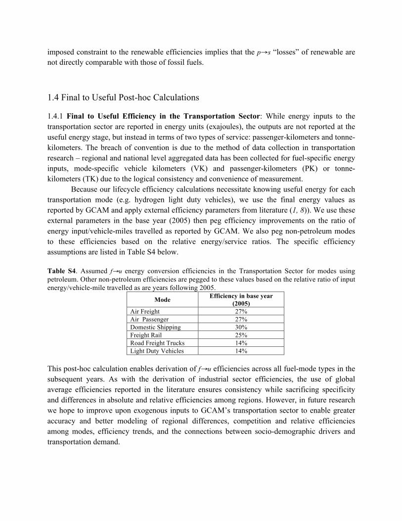
1.4 Final to Useful Post-hoc Calculations 1.4.1 Final to Useful Efficiency in the Transportation Sector: While energy inputs to the transportation sector are reported in energy units (exajoules), the outputs are not reported at the useful energy stage, but instead in terms of two types of service: passenger-kilometers and tonne-kilometers. The breach of convention is due to the method of data collection in transportation research – regional and national level aggregated data has been collected for fuel-specific energy inputs, mode-specific vehicle kilometers (VK) and passenger-kilometers (PK) or tonne-kilometers (TK) due to the logical consistency and convenience of measurement.
Because our lifecycle efficiency calculations necessitate knowing useful energy for each transportation mode (e.g. hydrogen light duty vehicles), we use the final energy values as reported by GCAM and apply external efficiency parameters from literature (1, 8)). We use these external parameters in the base year (2005) then peg efficiency improvements on the ratio of energy input/vehicle-miles travelled as reported by GCAM. We also peg non-petroleum modes to these efficiencies based on the relative energy/service ratios. The specific efficiency assumptions are listed in Table S4 below.
Table S4. Assumed f→u energy conversion efficiencies in the Transportation Sector for modes using petroleum. Other non-petroleum efficiencies are pegged to these values based on the relative ratio of input energy/vehicle-mile travelled as are years following 2005.
Mode Efficiency in base year (2005)
Air Freight 27% Air Passenger 27% Domestic Shipping 30% Freight Rail 25% Road Freight Trucks 14% Light Duty Vehicles 14%
This post-hoc calculation enables derivation of f→u efficiencies across all fuel-mode types in the subsequent years. As with the derivation of industrial sector efficiencies, the use of global average efficiencies reported in the literature ensures consistency while sacrificing specificity and differences in absolute and relative efficiencies among regions. However, in future research we hope to improve upon exogenous inputs to GCAM’s transportation sector to enable greater accuracy and better modeling of regional differences, competition and relative efficiencies among modes, efficiency trends, and the connections between socio-demographic drivers and transportation demand.

1.4.2 Final to Useful Efficiency in Industrial Sector: Many of GCAM’s f→u efficiency conversions in the industrial sector are indexed at 1.00 efficiency in the base year (1990/2005) and modeled as improving at an exogenously determined rate in each 15-year time step. In particular, the efficiencies of industrial energy services (represented by processes including energy use, cement production, and feedstock use) provided by four energy carriers (NG, refined liquids, hydrogen, and electricity) was indexed at 1.0 for 1990, electricity for cement production and feedstock use of NG, refined liquids, and coal was similarly normalized to a 1990 base year.
Using global average fuel-specific f→u conversion efficiencies reported for 1990 by Nakicenovic et al. (1) and taking fuel/energy carrier specific weighted averages of the energy inputs (in exajoules) for the three indexed processes (energy use, cement production, and feedstock use), we were able to ‘de-index’ the weighted average fuel-specific allocations for each fuel/energy-carrier. As shown in Table S5, this converts the indexed values into estimated efficiencies. Although this approach allowed us to fill in the missing pathways in industrial energy use, it requires the use of global average conversion efficiencies, and so may result in an underestimate of variability in industrial and, to a lesser degree, in overall energy efficiency across regions. However, no detailed regional data with global coverage using uniform and comparable methods was available, so we sacrificed regional specificity for uniformity of assumptions.
Table S5. Electricity, NG, and liquid subsector efficiencies were indexed in the GCAM output to 100% efficiency in the base year (1990). Values in the purpose boxes are the global average fuel-specific f→u conversion efficiencies reported for 1990 by Nakicenovic et al. (1). The weighted average energy inputs for each fuel/energy carrier type to various industry processes (energy use, feedstock, cement production) were de-inexed by assigning global average f→u efficiencies for the industrial sector reported by Nakicenovic et al. (1). Presumably, industrial electricity efficiencies are higher than average electricity accounting for T&D losses because industrial electricity is often generated on-site, and sometimes includes CHP.
1.4.3 Final to Useful Efficiency in Building Sector For heating/cooling services, coefficient of performance (COP) efficiency values were reported. COP includes the utilization energy
!"#$ %&'()*+ ,--. /..0 /.0.
!"#$"% &'(!)* +,- +,- ./-
012'(13456'7"758"95'%"246":$4";9* &'(0)* </- </- <=-
>? &'(>)* @'' @'' ,A-
B85C46"C"4D'(13456'EFG'8;2252* &'(B)* <.- <.- <<-
1$#234(2(35667#(8'3#96*:#4*8#6;(4<36$*76#;;(2(#)25 =*>(2#)?:(26#36*$@6,--0 A,B
'@'G56"H5%'585C46"C"4D'533"C"59CD &'(B)* IJ- IJ- I.-
C*<6D67#(8'3#96*:#4*8#6;(4<36$*76#;;(2(#)25 =*>(2#)?:(26#36*$@6,--0 E,B
'@'G56"H5%'K12'533"C"59CD &'(0)* <J- <J- <=-
'@'012'(B956KD'L25* "9%5M5% J//- J//- J/.-
'@'012'3;6'355%24;CN "9%5M5% J//- J//- J/.-
O5"KP45%')9%5M' "9%5M5% J//- J//- J/.-
F(G"(96D67#(8'3#96*:#4*8#6;(4<36$*76#;;(2(#)25 =*>(2#)?:(26#36*$@6,--0 HIB
'@'G56"H5%'8"#$"%'533"C"59CD &'(!)* +,- +,- ./-
'@'!"#$"%'(B956KD'L25* "9%5M5% J//- J/J- J/<-
'@'!"#$"%'3;6'355%24;CN "9%5M5% J//- J//- J/.-
O5"KP45%')9%5M' "9%5M5% J//- J//- J/.-

between inside and outside heat (thermal differentials) across device boundaries, thus the values can be higher than 100%. Clearly this value is not a thermodynamic efficiency for the device itself, nevertheless COP values of heating/cooling devices are included in the efficiency calculations for f→u energy conversions, and therefore increase the calculated efficiencies in the buildings sector over what they would be if system boundaries included only thermodynamic efficiencies for heating/cooling devices alone.
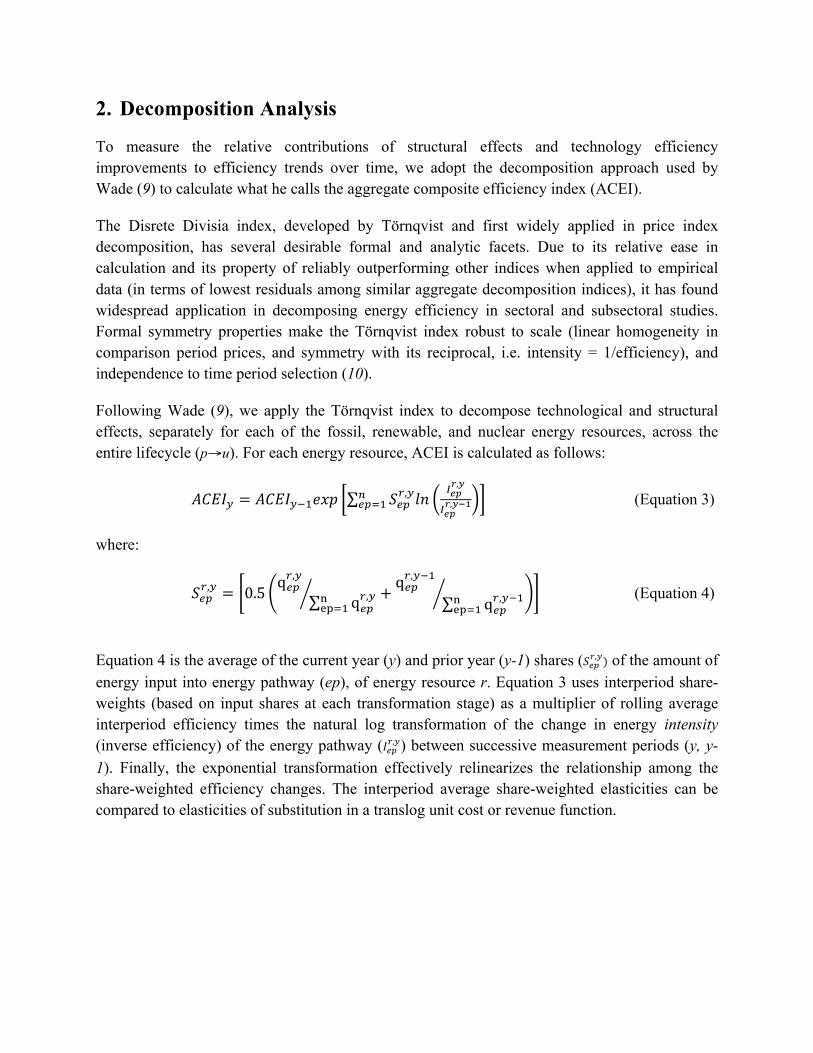
2. Decomposition Analysis
To measure the relative contributions of structural effects and technology efficiency improvements to efficiency trends over time, we adopt the decomposition approach used by Wade (9) to calculate what he calls the aggregate composite efficiency index (ACEI).
The Disrete Divisia index, developed by Törnqvist and first widely applied in price index decomposition, has several desirable formal and analytic facets. Due to its relative ease in calculation and its property of reliably outperforming other indices when applied to empirical data (in terms of lowest residuals among similar aggregate decomposition indices), it has found widespread application in decomposing energy efficiency in sectoral and subsectoral studies. Formal symmetry properties make the Törnqvist index robust to scale (linear homogeneity in comparison period prices, and symmetry with its reciprocal, i.e. intensity = 1/efficiency), and independence to time period selection (10).
Following Wade (9), we apply the Törnqvist index to decompose technological and structural effects, separately for each of the fossil, renewable, and nuclear energy resources, across the entire lifecycle (p→u). For each energy resource, ACEI is calculated as follows:
!"#$! = !"#$!!!!"# !!"!,!!"
!!"!,!
!!"!,!!!
!!"!! (Equation 3)
where:
!!"!,! = 0.5
q!"!,!
q!"!,!!
!"!!+q!"!,!!!
q!"!,!!!!
!"!! (Equation 4)
Equation 4 is the average of the current year (y) and prior year (y-1) shares (!!"!,!) of the amount of energy input into energy pathway (ep), of energy resource r. Equation 3 uses interperiod share-weights (based on input shares at each transformation stage) as a multiplier of rolling average interperiod efficiency times the natural log transformation of the change in energy intensity (inverse efficiency) of the energy pathway (!!"!,!) between successive measurement periods (y, y-1). Finally, the exponential transformation effectively relinearizes the relationship among the share-weighted efficiency changes. The interperiod average share-weighted elasticities can be compared to elasticities of substitution in a translog unit cost or revenue function.
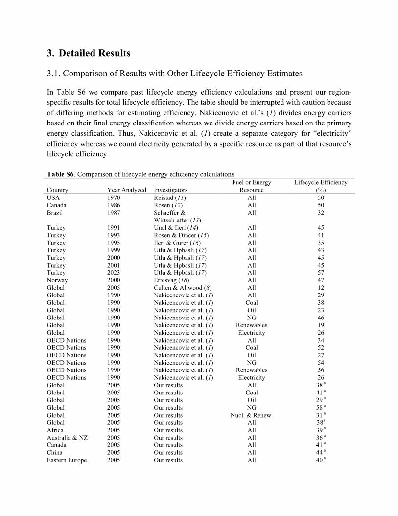
3. Detailed Results 3.1. Comparison of Results with Other Lifecycle Efficiency Estimates In Table S6 we compare past lifecycle energy efficiency calculations and present our region-specific results for total lifecycle efficiency. The table should be interrupted with caution because of differing methods for estimating efficiency. Nakicenovic et al.’s (1) divides energy carriers based on their final energy classification whereas we divide energy carriers based on the primary energy classification. Thus, Nakicenovic et al. (1) create a separate category for “electricity” efficiency whereas we count electricity generated by a specific resource as part of that resource’s lifecycle efficiency. Table S6. Comparison of lifecycle energy efficiency calculations Country Year Analyzed Investigators
Fuel or Energy Resource
Lifecycle Efficiency (%)
USA 1970 Reistad (11) All 50 Canada 1986 Rosen (12) All 50 Brazil 1987 Schaeffer &
Wirtsch-after (13) All 32
Turkey 1991 Unal & Ileri (14) All 45 Turkey 1993 Rosen & Dincer (15) All 41 Turkey 1995 Ileri & Gurer (16) All 35 Turkey 1999 Utlu & Hpbasli (17) All 43 Turkey 2000 Utlu & Hpbasli (17) All 45 Turkey 2001 Utlu & Hpbasli (17) All 45 Turkey 2023 Utlu & Hpbasli (17) All 57 Norway 2000 Ertesvag (18) All 47 Global 2005 Cullen & Allwood (8) All 12 Global 1990 Nakicencovic et al. (1) All 29 Global 1990 Nakicencovic et al. (1) Coal 38 Global 1990 Nakicencovic et al. (1) Oil 23 Global 1990 Nakicencovic et al. (1) NG 46 Global 1990 Nakicencovic et al. (1) Renewables 19 Global 1990 Nakicencovic et al. (1) Electricity 26 OECD Nations 1990 Nakicencovic et al. (1) All 34 OECD Nations 1990 Nakicencovic et al. (1) Coal 52 OECD Nations 1990 Nakicencovic et al. (1) Oil 27 OECD Nations 1990 Nakicencovic et al. (1) NG 54 OECD Nations 1990 Nakicencovic et al. (1) Renewables 56 OECD Nations 1990 Nakicencovic et al. (1) Electricity 26 Global 2005 Our results All 38 a Global 2005 Our results Coal 41 a Global 2005 Our results Oil 29 a Global 2005 Our results NG 58 a Global 2005 Our results Nucl. & Renew. 31 a Global 2005 Our results All 38a Africa 2005 Our results All 39 a Australia & NZ 2005 Our results All 36 a Canada 2005 Our results All 41 a China 2005 Our results All 44 a Eastern Europe 2005 Our results All 40 a

Former Soviet Union
2005 Our results All 43 a
India 2005 Our results All 35 a Japan 2005 Our results All 43 a Korea 2005 Our results All 45 a Latin America 2005 Our results All 35 a Middle East 2005 Our results All 37 a Southeast Asia 2005 Our results All 38 a USA 2005 Our results All 31 a Western Europe 2005 Our results All 42 a aAll scenarios have the same estimate lifecycle efficiency in the base year, 2005. Thus, this number is not tied to a specific scenario. 3.2. Scenario Description We analyze a range of scenarios examining the impacts of technology advancement and carbon policies on lifecycle energy efficiency and on primary fossil and non-fossil energy consumption. Technological change may progress at a conservative rate (REF), or at an advanced rate for end use technologies (ADV_EE) or both end-use and energy supply technologies (ADV_ALL). Carbon capture and storage (CCS) technologies may be implemented in scenarios involving carbon pricing. GCAM assumptions pertaining to advancements in different technologies are detailed in Clarke and Kyle (19). In addition to no carbon scenarios (business-as-usual, BAU), we also examine carbon pricing scenarios target reductions in greenhouse gas emissions to cap radiative forcing at 4.5/6.0 Watts per meter-squared in 2100. These scenarios are loosely based on representative concentration pathways (RCPs) 4.5/6.0 defined in Moss et al. (20) and Vuuren et al. (21). We model them by targeting CO2 concentrations of 530 and 660 ppm, respectively, in 2100 (22).
Table S7. Scenario description Scenario
Abbreviations Description
Business-as-usual (BAU) scenario group
Ref_Tech Reference technologies: The reference technology scenario includes substantial technological advances over currently available technology in almost every category.
Adv_EE Advanced end-use technologies: Assumes faster improvements in buildings, industrial and transportation sector technologies relative to reference scenario.
Adv_ALL Advanced end-use and non-fossil fuel supply technologies: Assumes rapid advances in end-use as well as energy supply technologies including nuclear, renewables, and hydrogen.
Moderate/aggressive climate policy scenario groups
RCP 4.5/6.0 Carbon pricing at levels that increase at a Hotelling schedule of 5% per year such that greenhouse gas concentrations reach radiative forcing potentials of 6.0 (moderate)/4.5 (aggressive) Watts per meter squared (W/m2) in 2100.
CCS Carbon Capture and Storage (CCS) is assumed in electricity generation, liquid fuel refining, hydrogen production, and cement manufacturing. CCS technologies operate only in scenarios involving carbon pricing.
Table S8. Scenario and the corresponding CO2 concentration levels, temperature rise and carbon prices.

Scenarios No carbon policy RCP 6.0 (Moderate Carbon Policy)
RCP 4.5 (Aggressive Carbon Policy)
Targeted radiative forcing in 2100 No target 6.0 Watts / m2 4.5 Watts / m2 Targeted GHG concentration levels in 2100 (a)
~850 ppm CO2-e ~650 ppm CO2-e
CO2 concentration levels in 2100 (b, c) 700 - 750 ppm CO2 ~660 ppm CO2 (targeted)
~530 ppm CO2 ((targeted))
Global mean temperature increase above pre-industrial levels (a)
~6 degrees C ~3.3 degrees C ~2.8 degrees C
Carbon Price (2005$/ton Carbon) in 2095 under Reference technology progression (d)
$210-$250 $485-$1000
Carbon Price (2005$/ton Carbon) in 2095 under Advanced technology progression (d)
$18-$27 $310-$630
Notes (a) Based on T. Masui et al (22). (b) Based on T. Masui et al (22) and D. P. v. Vuuren et al. (21) (c) The range of CO2 concentration levels for No Carbon Policy Scenarios represent advanced and reference
technological progress assumptions (d) The range of prices represent scenarios with and without CCS technologies (e) Converted according to 2005$ using price index reported in the ORNL Transportation Energy Data Book, 2011,
Appendix B 3.3 Results by Resource (BAU Scenario) Excel spreadsheet of all scenario results available at https://sites.google.com/site/gleemucd/
Figure S1a(left) and S1b(right): Share of coal primary energy used for each energy pathway from 1990-2100 (left) and lifecycle efficiency of each coal pathway from 1990-2100 (right) for the BAU Scenario.

Figure S2a(left) and S2b(right): Share of crude primary energy used for each energy pathway from 1990-2100 (left) and lifecycle efficiency of each crude pathway from 1990-2100 (right) for the BAU Scenario.
Figure S3a(left) and S3b(right): Share of natural gas primary energy used for each energy pathway from 1990-2100 (left) and lifecycle efficiency of each natural gas pathway from 1990-2100 (right) for the BAU Scenario.

Figure S4a(left) and S4b(right): Share of renewable and nuclear primary energy used for each energy pathway from 1990-2100 (left) and lifecycle efficiency of each renewable and nuclear primary energy pathway from 1990-2100 (right) for the BAU Scenario. 3.4 BAU Scenario Group Excel spreadsheet of all scenario results available at https://sites.google.com/site/gleemucd/
Figure S5a. BAU Scenario Description: Reference technology case technology (no advanced end-use or advanced non-fossil fuel supply). No CCS. No carbon policy.
Figure S5b. Adv_EE_noCCS Scenario Description: Advanced end-use technologies; faster improvements in a range of building- and industry- end-use technologies relative to reference technology scenario (19). No CCS. No carbon policy.

Figure S5c. Adv_All_noCCS Scenario Description: No carbon pricing and no CCS. Advanced end-use technologies and advanced non-fossil fuel supply technologies relative to reference technology scenario.
3.5 Moderate Climate Policies Group Excel spreadsheet of all scenario results available at https://sites.google.com/site/gleemucd/
Figure S5d. Ref_tech_no_CCS_RCP6.0 Scenario Description: Reference case technology (no advanced end-use or advanced non-fossil fuel supply). No CCS. Carbon pricing at levels that increase at a Hotelling schedule of 5% per year such that greenhouse gas concentrations reach radiative forcing of 6.0 Watts per meter squared (W/m2) in 2100.

Figure S5e. Adv_EE_noCCS_RCP6.0 Scenario Description: Advanced end-use technologies; faster improvements in a range of building- and industry- end-use technologies relative to reference technology scenario (19). No CCS. Carbon pricing at levels that increase at a Hotelling schedule of 5% per year such that greenhouse gas concentrations reach radiative forcing of 6.0 Watts per meter squared (W/m2) in 2100.
Figure S5f. Adv_EE_CCS_RCP6.0 Scenario Description: Advanced end-use technologies; faster improvements in a range of building- and industry- end-use technologies relative to reference technology scenario (19). CCS emerges in 2020. Carbon pricing at levels that increase at a Hotelling schedule of 5% per year such that greenhouse gas concentrations reach radiative forcing of 6.0 Watts per meter squared (W/m2) in 2100.

Figure S5g. Adv_All_noCCS_RCP6.0 Scenario Description: Advanced end-use technologies and advanced non-fossil fuel supply technologies relative to reference technology scenario. Carbon pricing at levels that increase at a Hotelling schedule of 5% per year such that greenhouse gas concentrations reach radiative forcing of 6.0 Watts per meter squared (W/m2) in 2100. No CCS.
Figure S5h. Adv_All_CCS_RCP6.0 Scenario Description: Carbon pricing at levels that increase at a Hotelling schedule of 5% per year such that greenhouse gas concentrations reach radiative forcing of 6.0 Watts per meter squared (W/m2) in 2100. CCS emerges in the year 2020. Advanced end-use technologies and advanced non-fossil fuel supply technologies relative to reference technology scenario.

Figure S5i. Ref_tech_CCS_RCP6.0 Scenario Description: Reference technology case technology (no advanced end-use or advanced non-fossil fuel supply). CCS emerges in 2020. Carbon pricing at levels that increase at a Hotelling schedule of 5% per year such that greenhouse gas concentrations reach radiative forcing of 4.5 Watts per meter squared (W/m2) in 2100.
3.6 Aggressive Climate Policies Group Excel spreadsheet of all scenario results available at https://sites.google.com/site/gleemucd/
Figure S5j. Ref_tech_CCS_RCP4.5 Scenario Description: Reference technology case technology (no advanced end-use or advanced non-fossil fuel supply). CCS emerges in 2020. Carbon pricing at levels that increase at a Hotelling schedule of 5% per year such that greenhouse gas concentrations reach radiative forcing of 4.5 Watts per meter squared (W/m2) in 2100.

Figure S5k. Ref_tech_no_CCS_RCP4.5 Scenario Description: Reference technology case technology (no advanced end-use or advanced non-fossil fuel supply). No CCS. Carbon pricing at levels that increase at a Hotelling schedule of 5% per year such that greenhouse gas concentrations reach radiative forcing of 4.5 Watts per meter squared (W/m2) in 2100.
Figure S5l. Adv_EE_noCCS_RCP4.5 Scenario Description: Advanced end-use technologies; faster improvements in a range of building- and industry- end-use technologies relative to reference technology scenario (19). No CCS. Carbon pricing at levels that increase at a Hotelling schedule of 5% per year such that greenhouse gas concentrations reach radiative forcing of 4.5 Watts per meter squared (W/m2) in 2100.

Figure S5m. Adv_EE_CCS_RCP4.5
Scenario Description: Advanced end-use technologies; faster improvements in a range of building- and industry- end-use technologies relative to reference technology scenario (19). CCS emerges in 2020. Carbon pricing at levels that increase at a Hotelling schedule of 5% per year such that greenhouse gas concentrations reach radiative forcing of 4.5 Watts per meter squared (W/m2) in 2100.
Figure S5n. Adv_All_noCCS_RCP4.5
Scenario Description: Advanced end-use technologies and advanced non-fossil fuel supply technologies relative to reference technology scenario. Carbon pricing at levels that increase at a Hotelling schedule of 5% per year such that greenhouse gas concentrations reach radiative forcing of 4.5 Watts per meter squared (W/m2) in 2100. No CCS.

Figure S5o. Adv_All_CCS_RCP4.5
Scenario Description: Carbon pricing at levels that increase at a Hotelling schedule of 5% per year such that greenhouse gas concentrations reach radiative forcing of 4.5 Watts per meter squared (W/m2) in 2100. CCS emerges in the year 2020. Advanced end-use technologies and advanced non-fossil fuel supply technologies relative to reference technology scenario.

3.6 Additional Figures 3.6.1 Comparison of results with and without Carbon Capture and Storage technologies. Below we examine the full range of efficiency and primary energy, first with and then without CCS becoming a feasible technology during the study period. Figure S6a shows the changing efficiencies and primary energy across fossil resources and nuclear/renewable resources for the reference scenario and the RCP 4.5 scenario at 15-year time steps. Figure S6b shows the same information for the same two scenarios, but in this case without CCS. Note that efficiencies of coal and NG resources increase in the scenario without CCS relative to the scenario with CCS, but that the total primary energy consumed across these pathways decreases markedly over time in the no CCS aggressive carbon policy, with energy being provided instead by nuclear/renewables. Energy conservation accounts for the rest of the difference in total energy between the reference and aggressive carbon policy scenarios. This high efficiency of natural gas is due to the effect of heat pumps, whose the efficiency is defined based on coefficient of performance or COP whose values can be greater than 1.
Figure S6a. Global lifecycle efficiencies and total primary energy use for all energy resources for the BAU scenario with reference technology (shaded) and for RCP 4.5 (aggressive carbon pricing policy case) with CCS (clear circles). The area of the circles indicates the amount of primary energy (p) for each energy resource. Nearly all other scenarios yield results that somewhere in between these two cases for both total primary consumption and efficiency.

Figure S6b. Global lifecycle efficiencies and total primary energy use for all energy resources for the BAU scenario with reference technology (shaded) and for RCP 4.5 (aggressive carbon pricing policy case) without CCS (clear circles). The area of the circles indicates the amount of primary energy (p) for each energy resource. Nearly all other scenarios yield results that somewhere in between these two cases for both total primary consumption and efficiency.

Developed vs. Developing Countries
Figure S7. Global lifecycle efficiencies of resources broken up by developing and developed countries in
2050 and 2095.
Change relative to Reference
ADV_ALL_CCS_RCP4.5ADV_EE_CCS_RCP4.5
ADV_ALL_NoCCS_RCP4.5
ADV_EE_NoCCS_RCP4.5
Ref_CCS_RCP4.5ADV_ALL_CCS_RCP6.0ADV_EE_CCS_RCP6.0
ADV_ALL_NoCCS_RCP6.0
ADV_EE_NoCCS_RCP6.0
Ref_CCS_RCP6.0Ref_NoCCS_RCP6.0
ADV_EE_NoCCS
Reference
0.4 0.5 0.6 0.7
Coal
2050
0.30 0.35 0.40 0.45 0.50
Crude
2050
0.60 0.65 0.70 0.75
NG2050
0.35 0.40 0.45 0.50 0.55
Nucl. & Renew
2050
0.40 0.45 0.50 0.55 0.60
Total Energy
2050
ADV_ALL_CCS_RCP4.5ADV_EE_CCS_RCP4.5
ADV_ALL_NoCCS_RCP4.5
ADV_EE_NoCCS_RCP4.5
Ref_CCS_RCP4.5ADV_ALL_CCS_RCP6.0ADV_EE_CCS_RCP6.0
ADV_ALL_NoCCS_RCP6.0
ADV_EE_NoCCS_RCP6.0
Ref_CCS_RCP6.0Ref_NoCCS_RCP6.0
ADV_EE_NoCCS
ReferenceCoal
2095
Crude
2095
NG
2095
Nucl. & Renew
2095
Total Energy
2095
DevelopedDeveloping
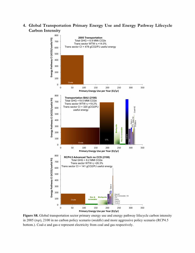
4. Global Transportation Primary Energy Use and Energy Pathway Lifecycle Carbon Intensity
Figure S8. Global transportation sector primary energy use and energy pathway lifecycle carbon intensity in 2005 (top), 2100 in no carbon policy scenario (middle) and more aggressive policy scenario (RCP4.5 bottom.). Coal-e and gas-e represent electricity from coal and gas respectively.
!"
#!!"
$!!"
%!!"
&!!"
'!!"
(!!"
)!!"
*!!"
!" '!" #!!" #'!" $!!" $'!" %!!" %'!"
!"#$%&'()*+,
)&'-.'/*-01234#536'(78'
($9:)$&'!"#$%&';4#'<#$'=#)$'/!72&$8'
Crude
2005 Transportation Total GHG = 6.9 MMt CO2e Trans sector WTW ! =14.0%
Trans sector CI = 478 gCO2/PJ useful energy
!"
#!!"
$!!"
%!!"
&!!"
'!!"
(!!"
)!!"
*!!"
!" '!" #!!" #'!" $!!" $'!" %!!" %'!"
!"#$%&'()*+,
)&'-.'/*-01234#536'(78'
($9:)$&'!"#$%&';4#'<#$'=#)$'/!72&$8'
Crude CTL C
oal-e
Nuc
& r
enew
able
Gas
G
as-e
G
as-H
2 G
TL
Coa
l-H2
Cru
de-e
Transportation BAU (2100) Total GHG =19.5 MMt CO2e Trans sector WTW ! =19.2%
Trans sector CI = 320 gCO2/PJ useful energy
Bio
liqui
ds
!"
#!!"
$!!"
%!!"
&!!"
'!!"
(!!"
)!!"
*!!"
!" '!" #!!" #'!" $!!" $'!" %!!" %'!"
!"#$%&'()*+,
)&'-.'/*-01234#536'(78'
($9:)$&'!"#$%&';4#'<#$'=#)$'/!72&$8'
Crude
RCP4.5 Advanced Tech no CCS (2100) Total GHG = 8.2 MMt CO2e Trans sector WTW ! =26.3%
Trans sector CI = 141 gCO2/PJ useful energy
Bioliquids
Coa
l-e
Nuc & renewable
Gas
G
TL
Gas
-e
Gas-H2 Nuc & renewable –H2 CTL Coal-e Coal-H2 Crude-e

5. Exergy Analysis: Assumptions and Results
“Exergy is a measure of the usefulness or value or quality of an energy form. Technically, exergy is defined using thermodynamic principles as the maximum amount of work which can be produced by a system or a flow of matter or energy as it comes to equilibrium with a reference environment” (23). Exergy efficiency is defined for a device as (24):
! =!"!#$% !"#$"#!"!#$% !"#$%
=!"#$ !"#$"#
!"#$!%! !"#$ !"#$"#
In this paper, exergy efficiency is estimated using quality factor multipliers determined in (1, 24) as:
! = ! × !
where v is a dimensionless quality factor used to correct for the loss of energy quality in the conversion process through the loses of water vapor (lower heating value), flue-gas, and the conversion to heat which is downgraded to be measured as mechanical work which has a lower quality factor (24). The lifecycle exergy efficiency is calculated in the same fashion as described in Equations 1 and 2 in the main text by substituting energy efficiency η with exergy efficiency !. The quality factors used in the paper are listed in the following Tables. Table S9. Assumed quality factors (!) for P→S conversions for electricity generation, fuels production and CHP.
Energy Resource QF Source
Electricity Generation Crude oil; Refined Liquids 0.94 (a)
NG 0.96 (a)
Coal 0.94 (a)
Biomass 0.90 (a)
Nuclear 1.00 (a)
Wind, Solar, Geothermal, etc. 1.00 (a)
Liquids Liquids from Crude 1.00 (a)
CTL, GTL 1.00 (a)
BTL, Ethanol 1.00 (b)
H2 All fuels 1.00 (b) CHP All fuels 0.64 (a)
(a) Based on Cullen and Allwood (24); Nakicenovic, Gill, and Kurz (1) (b) Assumed by authors
Table S10. Assumed quality factors (!) for F→U conversions in the transportation sector
Mode Technology / Fuel QF Sources Air Liquids 0.99 (a) Ship Liquids 0.95 (a) Rail Liquids 0.95 (a)

Electricity 0.93 (a)
Coal 1.00 (a)
Trucks Liquids 0.95 (a) LDV Liquids 0.97 (a)
Electricity 0.93 (a)
H2 1.00 (b)
Gas 0.93 (b)
Bus Liquids 0.95 (a)
Electricity 0.93 (a)
H2 1.00 (b)
Gas 0.93 (b)
(a) Based on Cullen and Allwood (24); Nakicenovic, Gill, and Kurz (1) (b) Assumed by authors
Table S11. Assumed quality factors (!) for F→U conversions in the building sector
Enduse service Fuel Device QF Sources Heat Biomass Furnace, Boiler 0.2 (a) (c)
Coal As above 0.31 (a) (c)
Gas Furnace, Water heater 0.21 (a) (c)
Stove 0.21 (a) (c)
Electricity Furnace 0.3 (a) (c)
Heat pump 0.3 (a) (c)
Water heaters 0.3 (a) (c)
Refined Liquids Furnace, water heaters 0.25 (a) (c)
Cooling Electricity Air conditioning 0.06 (b) (c) Lighting Electricity Incandascent 0.9 (a) (c)
fluorescent 0.9 (a) (c)
Appliances Electricity Various 0.9 (b) (c)
Gas Various 0.21 (a) (c)
(a) Based on Cullen and Allwood (24); Nakicenovic, Gill, and Kurz (1) (b) Assumed by authors (c) IEA Annex 49 (25).
Table S12. Assumed quality factors (!) for F→U conversions in the industrial sector
Enduse sector Fuel QF Sources Industrial Energy Use Biomass 0.39 (a)
Coal 0.39 (b)
Electricity 0.71 (b)
Gas 0.24 (b)
H2 0.71 (c)
Liquids 0.44 (b)
Process Heat Cement Biomass 0.31 (b)
Coal 0.31 (b)

Gas 0.21 (b)
Electricity 0.30 (b)
Liquids 0.25 (b)
H2 0.21 (d)
(a) Assumed same as coal (b) Based on Cullen and Allwood (24); Nakicenovic, Gill, and Kurz (1) (c) Assumed same as electricity (d) Assumed same as gas
Examples of lifecycle exergy efficiency calculation are provided in the table below.
Table S13. Examples of lifecycle exergy efficiency of gas to heat energy pathways and oil to transport vs. oil to heat pathways.
!! = !!×!!(fuel
transformation)
!! = !!×!!(electricity generation)
!! = !!×!!(end-use
device conversion)
!!(compound efficiency)
Gas → electricity → electric heater 93 38 (40×96) 24 (80×30) 7 Gas → Gas burner 91 100 13 (64×21) 12
Oil → Petro engine 93 100 12 (13×99) 12 Oil → Oil burner→ Heat 93 100 15 (61×25) 14
Where ! is the exergy efficiency; ! is the energy efficiency and ! is the quality factor. Examples are based on Tables 1, 3 and 5 of Cullen and Allwood (2010) for illustrative purpose and numbers in the table above may not be the same as those used in the paper.
The results of lifecycle exergy efficiencies by end-use sectors, decomposition analysis, and by primary resource by developed and developing countries are shown in Figures S9-11.
Figure S9. Lifecycle exergy efficiency by end use sector under three different climate scenarios (and with CCS under the aggressive climate policy scenario RCP4.5)
!"#
$"#
%!"#
%$"#
&!"#
&$"#
'!"#
'$"#
!"#$%#&'() *&%"(+,-) .,/&(01,+/21&)
345,'-)567#5&
7-)
()*#+,--./0!#+,--.#10$#--.10$#
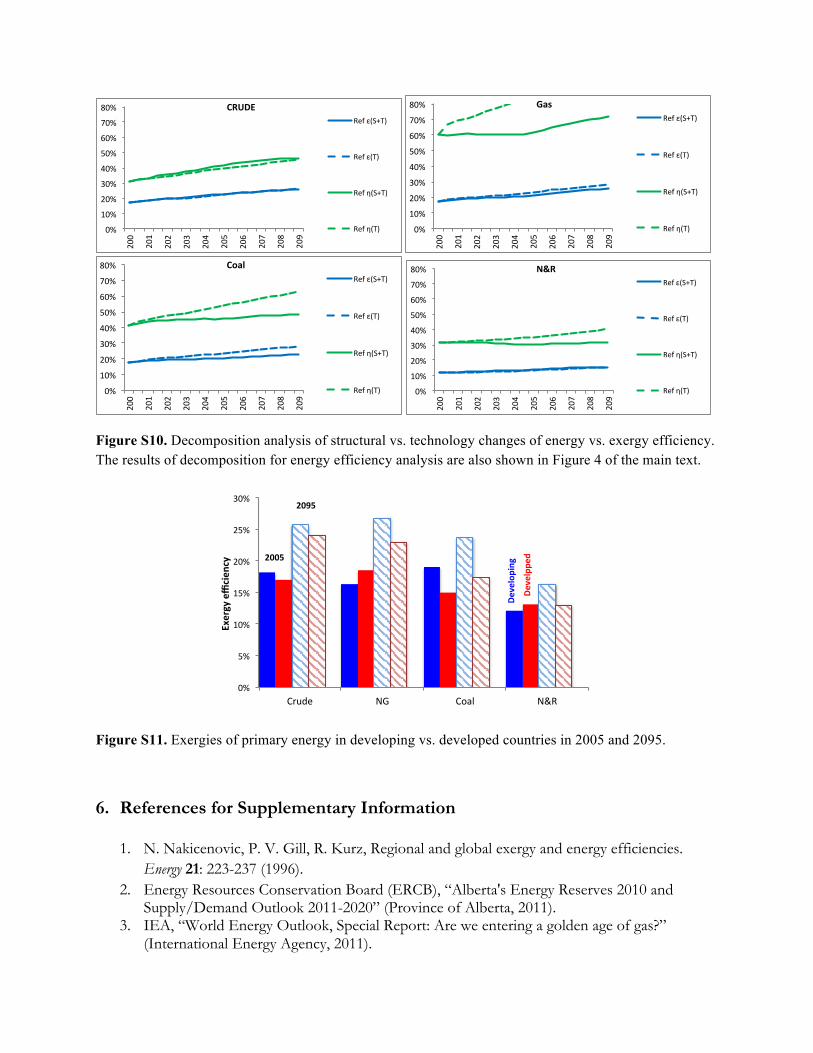
Figure S10. Decomposition analysis of structural vs. technology changes of energy vs. exergy efficiency. The results of decomposition for energy efficiency analysis are also shown in Figure 4 of the main text.
Figure S11. Exergies of primary energy in developing vs. developed countries in 2005 and 2095.
6. References for Supplementary Information
1. N. Nakicenovic, P. V. Gill, R. Kurz, Regional and global exergy and energy efficiencies. Energy 21: 223-237 (1996).
2. Energy Resources Conservation Board (ERCB), “Alberta's Energy Reserves 2010 and Supply/Demand Outlook 2011-2020” (Province of Alberta, 2011).
3. IEA, “World Energy Outlook, Special Report: Are we entering a golden age of gas?” (International Energy Agency, 2011).
!"#
$!"#
%!"#
&!"#
'!"#
(!"#
)!"#
*!"#
+!"#
%!!
%!$
%!%
%!&
%!'
%!(
%!)
%!*
%!+
%!,
!"#$%&-./#012345#
-./#0145#
-./#612345#
-./#6145# !"#
$!"#
%!"#
&!"#
'!"#
(!"#
)!"#
*!"#
+!"#
%!!
%!$
%!%
%!&
%!'
%!(
%!)
%!*
%!+
%!,
!"#$-./#012345#
-./#0145#
-./#612345#
-./#6145#
!"#
$!"#
%!"#
&!"#
'!"#
(!"#
)!"#
*!"#
+!"#
%!!
%!$
%!%
%!&
%!'
%!(
%!)
%!*
%!+
%!,
!"#$%-./#012345#
-./#0145#
-./#612345#
-./#6145# !"#
$!"#
%!"#
&!"#
'!"#
(!"#
)!"#
*!"#
+!"#
%!!
%!$
%!%
%!&
%!'
%!(
%!)
%!*
%!+
%!,
!"#$-./#012345#
-./#0145#
-./#612345#
-./#6145#
!"#
$"#
%!"#
%$"#
&!"#
&$"#
'!"#
()*+,# -.# (/01# -23#
!"#$%&'#()*#+
)&' ,--.'
,-/.'0#
1#234*+%'
0#1#244#
5'

4. M. Wang “GREET 1.8c” (Argonne National Laboratory, 2011). 5. EIA, “Annual Energy Review. Appendix F: Alternatives for Estimating Energy
Consumption” (U.S. Energy Information Administration, 2010). 6. H. D. Lightfoot, Understand the three different scales for measuring primary energy and
avoid errors. Energy 32: 1478-1483 (2007). 7. IEA, “ Key World Energy Statistics 2011” (International Energy Agency, 2011). 8. J. M. Cullen, J. M. Allwood, The efficient use of energy: Tracing the global flow of energy
from fuel to service. Energy Policy 38: 75-81 (2010). 9. S. H. Wade, “Measuring Changes in Energy Efficiency for the Annual Energy Outlook
2002” (Washington, DC, 2002). 10. B. Balk, W. E. Diewert, “A Characterization of the Törnqvist Price Index” (Department of
Economics, University of British Columbia, Vancouver, Canada, 2000). 11. G.M. Reistad, Available energy conversion and utilization in the United States. ASME J Eng
Power 97: 429-434 (1975). 12. M.A. Rosen, Evaluation of energy utilization efficiency in Canada using energy and exergy
analyses. Energy 17(4): 339-350 (1992). 13. R. Schaeffer, R.M. Wirtschafter, An exergy analysis for the Brazilian economy: from energy
production to final energy use. Energy 17(9): 841-855 (1992). 14. A. Unal, “Energy and exergy balance for Turkey in 1991” (University of Middle East
Technical University, Ankara, Turkey, 1994). 15. M.A. Rosen, I. Dincer, Sectoral energy and exergy modeling of Turkey. J. Energy Resour.
Technol. 119: 200-204 (1997). 16. A. Ileri, T. Gurer, Energy and exergy utilization in turkey during 1995, Energy 23(12): 1099-
1106 (1998). 17. Z. Utlu, A. Hepbasli, A Study on the evaluation of energy utilization efficiency in the
Turkish residential–commercial sector using energy and exergy analysis, Energy Buildings 35(11): 1145-1153 (2003).
18. I.S. Ertesvag, Energy, exergy, and extended-exergy analysis of the Norwegian society 2000. Energy 30(5): 649-675 (2005).
19. Clarke, L., P. Kyle, et al. (2008). CO2 Emissions Mitigation and Technological Advance: An Updated Analysis of Advanced Technology Scenarios (Scenarios Updated January 2009), Pacific Northwest National Laboratory.
20. R. H. Moss et al., The next generation of scenarios for climate change research and assessment. Nature 463(7282): 747-756 (2010).
21. D. P. v. Vuuren et al., The representative concentration pathways: an overview. Climatic Change 109:5-31. doi: DOI 10.1007/s10584-011-0148-z (2011).
22. T. Masui et al., An emission pathway for stabilization at 6 Wm^−2 radiative forcing. Climatic Change 109:59-76. doi: DOI 10.1007/s10584-011-0150-5 (2011).
23. Rosen, M.A., I. Dincer, and M. Kanoglu, Role of exergy in increasing efficiency and sustainability and reducing environmental impact. Energy Policy, 36(1): 128-137 (2008).
24. Cullen, J.M. and J.M. Allwood, Theoretical ef!ciency limits for energy conversion devices. Energy, 35: 2059-2069 (2010).
25. ECBCS Annex 49, Low Exergy Systems for High-Performance Buildings and Communities: Exergy Assessment Guidebook for the Built Environment, 2011, Fraunhofer IBP.
