In the format provided by the authors and unedited.

Regionally strong feedbacks 1

between the atmosphere and terrestrial biosphere 2

Supplementary Information 3

Julia K. Green1*, Alexandra G. Konings1,2, Seyed Hamed Alemohammad1,3, Joseph Berry4, 4

Dara Entekhabi3,5, Jana Kolassa6,7, Jung-Eun Lee8, Pierre Gentine1,9 5

1 Department of Earth and Environmental Engineering, Columbia University, New York,

NY.

2 Department of Earth System Science, Stanford University, Stanford, CA.

3 Department of Civil and Environmental Engineering, Massachusetts Institute of

Technology, Cambridge, MA.

4 Department of Global Ecology, Carnegie Institution of Washington, Stanford, CA.

5 Department of Earth, Atmospheric and Planetary Sciences, Massachusetts Institute of

Technology, Cambridge, MA.

6 University Space Research Association, Columbia, MD.

7 Global Modeling and Assimilation Office, NASA Goddard Space Flight Center, Greenbelt,

MD.

8 Department of Earth, Environment and Planetary Sciences, Brown University, Providence,

RI.

9 The Earth Institute, Columbia University, New York, NY.

*Correspondence to: jg3405@columbia.edu.

Regionally strong feedbacks between theatmosphere and terrestrial biosphere

© 2017 Macmillan Publishers Limited, part of Springer Nature. All rights reserved.

SUPPLEMENTARY INFORMATIONDOI: 10.1038/NGEO2957

NATURE GEOSCIENCE | www.nature.com/naturegeoscience 1

Supplementary Tables and Figures 6

Supplementary Table 1. 7

Modeling Center

(or Group) Institute ID Model Name

Beijing Climate Center,

China Meteorological Administration BCC BCC-CSM1.1

College of Global Change and Earth System

Science, Beijing Normal University GCESS BNU-ESM

Canadian Centre for Climate

Modelling and Analysis CCCMA CanESM2

National Center for Atmospheric Research NCAR CCSM4

Centro Euro-Mediterraneo per I

Cambiamenti Climatici CMCC CMCC-CESM

NOAA Geophysical Fluid Dynamics

Laboratory NOAA GFDL GFDL-ESM2M

NASA Goddard Institute for Space Studies NASA GISS GISS-E2-H

Met Office Hadley Centre (additional

HadGEM2-ES realizations contributed by

Instituto Nacional de Pesquisas Espaciais)

MOHC (additional

realizations by

INPE) HadGEM2-ES

Institute for Numerical Mathematics INM INM-CM4

Institut Pierre-Simon Laplace IPSL

IPSL-CM5A-LR

IPSL-CM5A-MR

Max-Planck-Institut für Meteorologie

(Max Planck Institute for Meteorology) MPI-M

MPI-ESM-MR

MPI-ESM-LR

8

9

Supplementary Fig. 1. Biosphere-atmosphere correlations. Latent heat flux and SIF (a), 10

GPP and SIF (b), sensible heat flux and SIF (c), and sensible heat flux and boundary layer 11

height (d). Heat flux and GPP data are from Fluxnet-MTE while boundary layer height data 12

is from ERA-Interim. In a-c, a correlation that is close to +1/-1 signifies that the sensible heat 13

flux, latent heat flux, or GPP is proportional to the biosphere flux. To isolate the growing 14

season, time series points are used if their SIF values are greater than or equal to half the 15

maximum monthly climatology for the year. 16

17

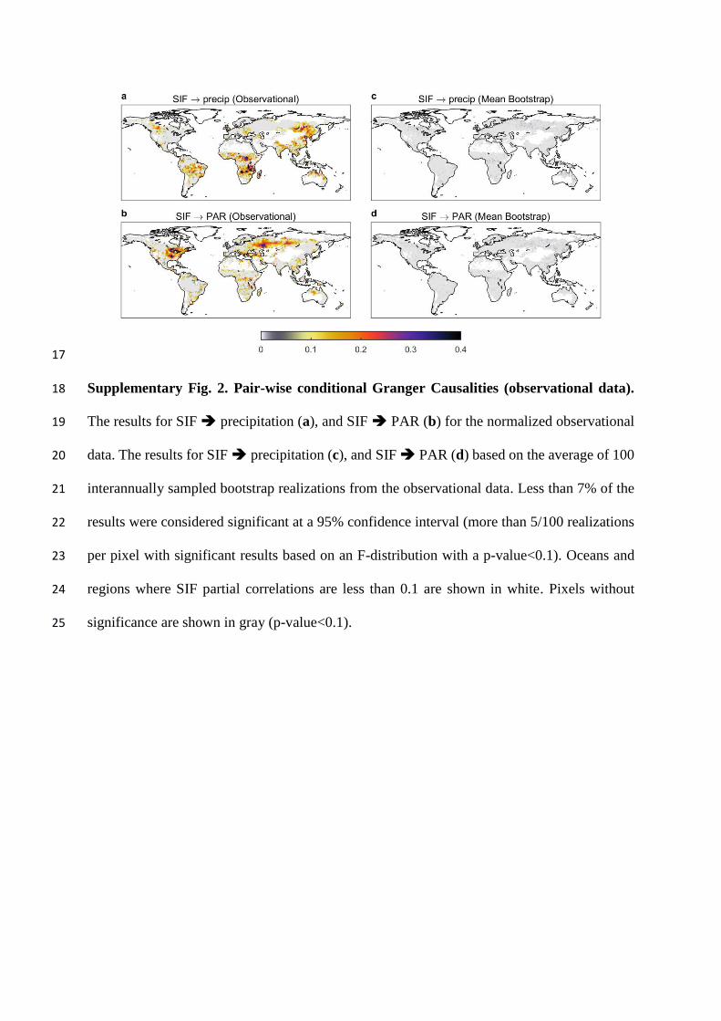
Supplementary Fig. 2. Pair-wise conditional Granger Causalities (observational data). 18

The results for SIF precipitation (a), and SIF PAR (b) for the normalized observational 19

data. The results for SIF precipitation (c), and SIF PAR (d) based on the average of 100 20

interannually sampled bootstrap realizations from the observational data. Less than 7% of the 21

results were considered significant at a 95% confidence interval (more than 5/100 realizations 22

per pixel with significant results based on an F-distribution with a p-value<0.1). Oceans and 23

regions where SIF partial correlations are less than 0.1 are shown in white. Pixels without 24

significance are shown in gray (p-value<0.1). 25

26

Supplementary Fig. 3. Pair-wise conditional Granger causality separated by frequency. 27

The first column is for the SIF on precipitation signal, divided into its subseasonal (below 3 28

months) (a), seasonal (between 3 and 12 months) (b), and interannual (> 1 year) (c) 29

components. The second column is for the SIF on PAR signal, divided into its subseasonal (d), 30

seasonal (e), and interannual (f) components. Oceans and regions where SIF partial correlations 31

are less than 0.1 are shown in white. Pixels without significance are shown in gray (p-32

value<0.1). 33

34

Supplementary Fig. 4. PAR, cloud fraction and precipitation correlations. Correlation of 35

PAR and low-level clouds (a), PAR and mid-level clouds (b), PAR and high-level clouds (c), 36

and PAR and precipitation (d). To isolate the growing season and control for top of 37

atmosphere radiation, time series points are used if their SIF values are greater than or equal 38

to half the maximum monthly climatology for the year. Cloud data is from the CERES 39

ISCCP-D2-like product. 40

41

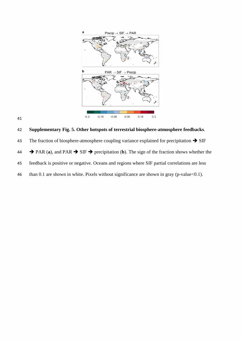
Supplementary Fig. 5. Other hotspots of terrestrial biosphere-atmosphere feedbacks. 42

The fraction of biosphere-atmosphere coupling variance explained for precipitation SIF 43

PAR (a), and PAR SIF precipitation (b). The sign of the fraction shows whether the 44

feedback is positive or negative. Oceans and regions where SIF partial correlations are less 45

than 0.1 are shown in white. Pixels without significance are shown in gray (p-value<0.1). 46

47

Supplementary Fig. 6. Comparison of significant observational and Earth System 48

Model results for forcings. Boxplots showing the distributions of observational and model 49

results for atmospheric forcings (a,c) and biospheric forcings (b,d). Boxes are defined by the 50

upper quartile, median and lower quartile of the data while whiskers are defined by the 51

outliers. Only significant pixels are represented (p-value<0.1). 52

53

Supplementary Fig. 7. Earth system model precipitation GPP precipitation 54

fractions of variance explained. Only significant pixels are shown (p-value<0.1). 55

56

Supplementary Fig. 8. Earth system model PAR GPP PAR fractions of variance 57

explained. Only significant pixels are shown (p-value<0.1). 58

59

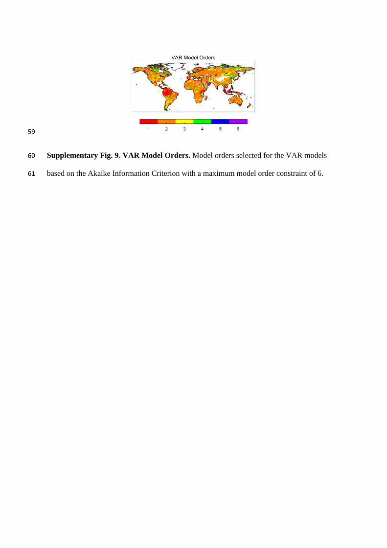
Supplementary Fig. 9. VAR Model Orders. Model orders selected for the VAR models 60

based on the Akaike Information Criterion with a maximum model order constraint of 6. 61

62

Supplementary Fig. 10. Pairwise-conditional Granger causality tests for all synthetic 63

time series trials. The results for the causal test (a), the non-causal test (b), the bootstrapping 64

test (c), and the causal test with an additional causal link between SIF and PAR (d). 65

Magnitude is shown in the top row with the significance test on the bottom (black means that 66

we can reject the null hypothesis of 0 causality at p-value<0.05, white means that we cannot). 67

The pairwise conditional metric represents the fraction of explained variance when omitting 68

the variable compared to the full model (in log scale), i.e. 69

Si, j = - lnvar(model of variable i omitting variable j)

var(full model of variable i)

æ

èçö

ø÷. 70