supplementary information - harvard...
TRANSCRIPT
W W W. N A T U R E . C O M / N A T U R E | 1
SUPPLEMENTARY INFORMATIONdoi:10.1038/nature12962
Index to Supplementary Results and Methods 1. Fly rearing and developmental staging 2 2. Dissection of Organ Systems 2-3 2A. Larval tissue Dissections 2 2B. L3 Imaginal Discs mass preparation 2 2C. Fly WPP and 2-day old pupae CNS 2 2D. White pre-pupal salivary gland and fat body 2 2E. Pupal fat body mass preparation 2 2F. Adult gonads and reproductive tissues 2 2G. Adult gut and carcass 3 2H. Adult head 3 3. Environmental Perturbations 4-5 3A. Heat Shock 4 3B. Cold Shock1 4 3C. Cold Shock 2 4 3D. Feeding schedule for consumed treatments 4-5 3D1. Treatment schedule for Larvae 4 3D2. Treatment schedule for Adults 4 3D3. Caffeine feeding 4 3D4. Copper feeding 5 3D5. Zinc feeding 5 3D6. Cadmium feeding 5 3D7. Paraquat feeding 5 3D8. Rotenone feeding 5 3D9. Resveratrol feeding 5 4. Cell Lines 55. RNA Isolation 5-6 6. Illumina RNA-seq library construction and sequencing 6 7. Illumina CAGE library construction and sequencing 6 8. polyA-seq: RNA sequencing of polyadenylation sites 6 9. 454 Titanium-platform RNA-seq library construction and
sequencing 6-7
10. 454 read mapping 7 11. cDNA capture and sequencing 7 12. Read mapping and filtering 7-8
13. Building transcript models from CAGE,RNA-seq, EST, cDNA and poly (A) sequence data 8-9
14. Predicting proteins based on transcript models 9-10 15. siRNA analysis 10 16. Identifying conserved domains in predicted proteins 10 16A Conserved Domain and GO analysis of complex loci 10 17. Identifying conserved ORFs that lack known domains 10 18. Defining lncRNA elements 11 19. MISO analysis of splicing dynamics 11 19A Detailed analysis of sex-specific splicing in somatic tissues 11 20. Computing Gene Expression 11 21. Differential Gene Expression Analysis 12 22. Statistical methods 12 23. Supplementary Table Legends 13 24. List of Supplementary Data Files 13 25. Supplementary References 14-15 26. Supplementary Figures 16-25

SUPPLEMENTARY INFORMATION
2 | W W W. N A T U R E . C O M / N A T U R E
RESEARCH
Supplementary Methods 1. Fly rearing and developmental staging Fly stocks (except where specified, the sequenced D. melanogaster isogenic strain y1 cn1 bw1 sp1 was used1) were reared at 24° C on standard Drosophila medium (http://flystocks.bio.indiana.edu/Fly_Work/media-recipes/media-recipes.htm). To collect larvae and adults, the flies were raised in 250 ml bottles containing 40 ml medium. To aid in staging third instar larvae the medium contained 0.05% bromphenol blue (BPB2) and staging was done as described3.
Synchronized embryos were collected from large population cages (ca. 25 cm x 25 cm x 25 cm; maintained at 24° C on a cycle of 14 h light 10 h dark) from adults that were less than one week old. Following at least one – 2 h pre-lay that preceded timed collections each day, embryos were collected for two hours on three hard egg lay collection plates made in 150 X 15 mm Petri dishes containing a substrate of 3.3% agar, 13% unsulfured molasses, and 0.15% Tegasept. The hard egg lay plates were completely covered with a thin layer of moist yeast paste (Fleischmann’s Baker’s Dry Yeast) and placed horizontally on a short 1 cm raised Plexiglas bar in the bottom of each cage to avoid crushing flies. Staged embryos were passed through an 850 micron screen and collected on a 75 micron screen to remove adults and yeast paste. Embryos were then dechorionated by treatment with a solution of 50% bleach (3% sodium hypochlorite), 0.2% sodium chloride, and 0.02% Triton-X-100 for five minutes. Embryos were washed twice with 0.2% NaCl, 0.02% Triton buffer and split into two samples. Most of the sample (approximately 95%) was rinsed with de-ionized water in a buchner funnel under mild vacuum, dried briefly, immediately frozen on dry ice and stored at -80˚ C for RNA preparations. The small aliquot was transferred to a clean tube and fixed (0.1 M Pipes (pH 6.9), 2 mM EGTA, 1 mM MgSO4, 4% paraformaldehyde, 0.1% glutaraldehyde and 50% heptane for staging4. Samples were shaken for five minutes in the fixative, centrifuged briefly and the aqueous fraction was removed. An equal volume of methanol containing 2 mM EGTA was added and the sample was shaken for five additional minutes. Tissue was washed twice in methanol with 2 mM EGTA and saved at -80˚C for the characterization of developmental stages.
2. Dissection of Organ Systems To detect rarely expressed and tissue specific RNAs we dissected organ systems from larval, pupal and adult animals. We examined components of the nervous system, from larval and pupal brains and ventral ganglia and from aged 1, 4 and 20-day adult heads (primarily brain) of mated males and virgin and mated females. To interrogate the reproductive system we dissected ovaries from females and testes and accessory glands from males. To study the digestive system we examined larval and pupal salivary glands and larval and aged 1, 4 and 20-day adult midgut, hindgut and malpighian tubules. We dissected larval and pupal fat body the primary metabolic and detoxification organ performing functions analogous to the human liver. To study the epidermis and muscle organ systems, we mass isolated larval imaginal discs adapted from a previously describe approach2, with modifications detailed below and an aliquot of the sample prep is shown in Supplementary Figure 8. We also dissected larval and aged 1,4 and 20-day adult carcasses, which contain cuticle, epidermis, muscle and oenocytes as well as peripheral neurons. All tissues were stored at -80˚ C immediately after dissection until sufficient material had been collected to permit RNA preparations. A yield of approximately 4 µg total RNA per mg of tissue collected was typical. A cartoon giving the anatomical relationships between the tissues collected is provided in Supp. Fig. 10. Specifics follow:
2A. Larval tissue dissections: Bottles were started with approximately 60 adult OreR flies at 25˚ C. After 5 days, climbing third instar larvae were collected and transferred to a dissecting surface with 1X PBS buffer (Ambion) for dissections. We identified the sex of the larva by the presence of the large clear spherical testes (or smaller ovary) embedded in the white fat body on the lateral sides of the A5 segment. We recorded and collected the tissues with equal representation of each sex. To dissect, the cuticle was torn immediately posterior to the mouth hooks using paired forceps and the larvae were everted as with WPP dissections. The digestive system and fat body were pulled toward the anterior end and away from the cuticle. The digestive system was disconnected from the body immediately anterior to the proventriculus. The salivary glands were collected by pinching them off from the attached fat body. The extensive and reticulated fat body was removed from the carcass and digestive system. The trachea were removed from the digestive system and collected with the carcass. Tissues collected included the gut (fat body removed, Malphigian tubules included), the salivary glands (with as much fat body removed as possible), and carcass (without the guts, salivary glands, fat

W W W. N A T U R E . C O M / N A T U R E | 3
SUPPLEMENTARY INFORMATION RESEARCH
body and gonads). Dissections were done concurrently so that all three tissues were collected from a single animal. Male and female tissues were collected in separate tubes and mixed in equal numbers for the RNA preparations.
2B. L3 Imaginal Discs mass preparation: Bulk preparations of imaginal disc tissue were done as previously described5 with the following modifications. First instar larvae were transferred to ventilated plastic chambers containing seventeen feet of cotton rope saturated in a protein-rich yeast slurry (200 g active dry yeast, 6 oz Gerber’s Banana food, 100 ml Grapefruit juice, 50 g ground Special K, 40 g Gerber’s Baby Cereal, 20 g Wheat Germ, 1200-1400 ml water) and were allowed to grow until wandering larvae were observed. Larvae were ground with a Kitchen Aid Artisan mixer (Model KSM150SPER) and Kitchen Aid grain mill attachment (Model KGMA) with the plates set to leave about 5% of the total larvae unground. Ringer’s solution was replaced with Organ Medium (25 mM β-Glycerol phosphate disodium salt pentahydrate (Fluka 50020), 10 mM KH2PO4, 30 mM KCl, 10 mM MgCl2, 3 mM CaCl2, 162 mM sucrose) at all steps. A photograph of the isolated tissues is given (Supplementary Fig. 9).
2C. Fly WPP and 2-day old pupae CNS: Staged WPP and 2-day old pupae were dissected in PBS (phosphate buffered saline). The posterior end of the pupa was removed with two forceps at the A7 abdominal segment. The anterior body of the pupa was removed from the pupal case with forceps. We held each cuticle at the anterior tip and gently teased the body towards the posterior opening with forceps. We pulled the cuticle from the anterior end through the second forceps, holding them nearly closed around the vacated cuticle. This squeezed the body of the pupa out of the cuticle. The yellow eye discs were removed from the brain lobes of the CNS. The connected antennal segment at the anterior margin of the brain was removed. The developing leg and wing disc tissue along with the fat body was removed, and the attached subesophageal ganglion and ring gland were recovered along with the brain. The CNS and ring gland were transferred to a collection tube on dry ice and then stored at -80˚ C until sufficient tissue for RNA isolation was collected.
2D. White pre-pupal salivary gland and fat body: We collected white pre-pupae (WPP) as in Graveley et al. 3 and dissected in PBS buffer. We identified the sex of the larva by the presence of the large clear spherical testes (or smaller ovary) embedded in the white fat body on the lateral sides of the A5 segment. We recorded and collected the tissues with equal representation of each sex. We note that the female WPP tend to be larger. We tore the cuticle immediately posterior to the mouth hooks and then everted the WPP by pushing the posterior end inside the body cavity with closed forceps, and finally collected the fat body and salivary glands in separate tubes on dry ice.
2E. Pupal fat body mass preparation: We transferred WPP animals 48 h after staging and resting at 25° C to a 15 ml polycarbonate falcon tube. We added 2 ml of Drosophila Ringers (182 mM KCl, 46 mM NaCl, 3 mM CaCl, 10 mM Tris-HCl pH 7.2) containing 2% Ficoll, and crushed the pupae in the tube to release contents from the cuticles. We added 5 ml of Ringers with 2% Ficoll, mixed with a large bore disposable pipet and filtered through a 100 um screen. The cell suspension was centrifuged at 660xG for 10 minutes at 40°C, and fat body cells were collected from the surface of the buffer and transferred to a 1.5ml eppendorf tube. Cell suspensions were centrifuged at 660xG for 5 minutes at 40° C to remove as much of the buffer from beneath the cells as possible. We froze the fat body cells by placing them on dry ice and stored at -80° C for RNA preparation.
2F. Adult gonads and reproductive tissues: Staged adult flies were anesthetized with CO2 for 30 minutes or less while dissections were done in PBS (1X; Ambion) for less than 10 minutes each. To dissect/open the abdomen, we pinned down the thorax on either side with a set of surgical steel forceps (size #4 or #5), and pulled the T3 legs posteriorly to remove the overlying cuticle and expose the digestive and reproductive organs. The reproductive tissues were removed and separated from the digestive tract and the cuticle. In the females, the reproductive tissues included the ovaries and their attached oviducts. Due to tearing and mechanical damage during dissection, the oviducts were incompletely recovered. In the males, the reproductive tissues included the testes (generally bright yellow), and the accessory glands (generally translucent, with incomplete recovery of the attached seminal vesicle). We collected the ovaries and oviducts together as a single sample, and separated the testes from the accessory glands for independent RNA isolation and sequencing. These tissues were dissected away from all other attached cells, and then frozen in 1.5 ml tubes submerged in dry ice, and then stored at -80˚ C until sufficient quantities were obtained for RNA purifications.

SUPPLEMENTARY INFORMATION
4 | W W W. N A T U R E . C O M / N A T U R E
RESEARCH
2G. Adult gut and carcass: Adult flies were staged and anesthetized as for the gonad preparation. The digestive tracts and carcasses were separated after removing the head and discarding. Holding the thorax and pulling the T3 legs posteriorly to expose the digestive and reproductive organs was used to dissect the abdomen. The reproductive tissues were removed and discarded. The digestive tract was separated from the cuticle, adipose tissue (fat body) and other tissues, and then frozen on dry ice. The remaining tissues (without the head and reproductive organs) were frozen on dry ice and designated the carcass. All tissues were stored at -80˚ C until sufficient quantities were obtained for RNA purifications.
2H. Adult head: Isolation of the fly heads was accomplished by placing CO2-anesthitized adults in a 15 ml conical tube that was then flash frozen in liquid nitrogen for about one minute. The tube was then shaken vigorously for 10 seconds, and tapped on the bench-top. The broken flies were placed in a frozen glass petri dish on dry ice. The frozen severed heads were removed with dissecting forceps and placed in an eppendorf tube on dry ice. Flies were processed in groups of 100 animals per dissection. Isolated tissue was stored at -80˚ C until RNA could be purified from an adequate number of prepared heads. Typically, heads were missing the antennal and maxillary organs, while the mouth-parts were retained.
3. Environmental Perturbations 3A. Heat Shock: Twenty virgin males and 20 virgin females were maintained on standard corn meal agar at 25°C for four days. After four days the 40 adult flies were transferred to clean glass vials and placed in a 36° C water bath (wet heat) and held at 36°C for 1 hour followed by a 30-minute recovery at 25° C prior to freezing in liquid nitrogen. This treatment produced relatively high lethality due to excessive moisture buildup in the vials.
3B. Cold Shock1: Newly eclosed flies were collected, and placed in cornmeal agar food vials containing 20 males and 20 females were and kept at 25° C for 84 hours. Aged, mated flies were transferred to empty glass vials and placed in a micro-cooler water bath containing 10% glycol at 25° C. The temperature was decreased to 0°C at a rate of 0.2°C per minute and then flies were held at 0° C for 9 hours. After the cold treatment flies were transferred to fresh food vials and kept at 25° C for 2 hours for the recovery period. Following recovery flies were placed in 2 ml tubes, flash frozen in liquid nitrogen and stored at -80° C prior to RNA preparations.
3C. Cold Shock 2: Flies were treated as in “Cold Shock 1”, above, except flies were held on food vials for four days. Aged, mated flies were transferred to empty glass vials and placed in a micro-cooler water bath containing 10% glycol at 0° C for two hours. Following the cold shock flies were transferred to fresh food vials and kept at 25° C for 30 minutes for the recovery period. Following recovery flies were placed in 2 ml tubes, flash frozen in liquid nitrogen and stored at -80° C prior to RNA preparations.
3D. Feeding schedule for consumed treatments:
3D1. Treatment schedule for Larvae: For each treatment, approximately 50 (mixed sex) young mated adults were transferred to each fresh food vials and maintained for 12 hours. Vials were cleared and allowed to age 3.5 to 4 days. Vials were then rinsed into a series of sieves using tepid water; feeding third instar larvae were collected form the #40 sieve and transferred to a hard agar plate with a pot of yeast to induce crawling. Prior to reaching the yeast, larvae were captured and 50 larvae were transferred to new food vials containing the treatment of interest (details below), and larvae were allowed to feed for 4 hours. Treated larvae were captured and transferred to 2 ml vials, flash frozen in liquid nitrogen and stored at -80° C prior to RNA preparations. The number of survivors was recorded and the mean lethality calculated for each treatment.
3D2. Treatment schedule for Adults: For each treatment, 40 newly eclosed males and females (1:1) were transferred to fresh food (BDSC corn meal agar) vials and maintained at 25° C for two days. To treat flies, two Kimwipes were folded into a square and put in the bottom of a one-pint glass bottle. Kimwipes were saturated with 4 ml of the treatment solution, (10% sucrose solution and one drop of green vegetable coloring per 50 ml solution, plus the treatment of interest). Harvesting time for adults varied by treatment. Upon harvesting, flies were placed in 2 ml tubes, flash frozen in liquid nitrogen and stored at -80° C prior to RNA preparations.
3D3. Caffeine feeding: Starved larvae (as above) were transferred to food vials containing 1.5 mg/ml caffeine and allowed to feed for 4 h. Adults fed 25 mg/ml caffeine were harvested after 8 h; adults fed 2.5 mg/ml caffeine were harvested after 48 h, and after 24 h an additional 1 ml of treatment solution was dripped onto the Kimwipe. Upon harvesting, flies were placed in 2 ml tubes, flash frozen in liquid nitrogen and stored at -80° C
W W W. N A T U R E . C O M / N A T U R E | 5
SUPPLEMENTARY INFORMATION RESEARCH
prior to RNA preparations. For adults, 2.5 mg/ml caffeine is near the LD50 for a 48 h treatment. 25 mg/ml caffeine is 100% lethal after 24 h.
3D4. Copper feeding: Starved larvae were transferred to new food vials containing 0.5 mM CuSO4 and allowed to feed for 12 h. The number of survivors was recorded and the mean lethality calculated for each treatment. Adults were fed with 15 mM CuSO4. After 24 h an additional 1 ml of the treatment solution was dripped onto the Kimwipe. Flies were harvested after 48 h of feeding, placed in 2 ml tubes, flash frozen in liquid nitrogen and stored at -80° C prior to RNA preparations. Adult concentrations were all done at or near the LD50 determined for our feeding method after 48 h. Adults were fed 15 mM copper for 48 h.
3D5. Zinc feeding: Starved larvae were transferred to new food vials containing the 5 mM ZnCl2 and allowed to feed for 12 h. Treated larvae were transferred to 2 ml vials, flash frozen in liquid nitrogen and stored at -80° C prior to RNA preparations. Adults were fed with 4.5 mM ZnCl2. After 24 h an additional 1 ml of the treatment solution was dripped onto the Kimwipe. Flies were harvested after 48 h of feeding, placed in 2 ml tubes, flash frozen in liquid nitrogen and stored at -80° C prior to RNA preparations. Adult concentrations were done at or near the LD50 determined for our feeding method after 48 h. Adults were fed 4.5 mM zinc for 48 h. Zinc appears to cause a neuromuscular defect in both adults and larvae.
3D6. Cadmium feeding: Starved larvae were transferred to new food vials containing 0.05 mM CdCl2 and allowed to feed for 6 or 12 h. Treated larvae were transferred to 2 ml vials, flash frozen in liquid nitrogen and stored at -80° C prior to RNA preparations. Adults were fed with 0.1 mM or 0.05 mM CdCl2. After 24 h an additional 1 ml of solution was dripped onto the Kimwipe. Flies were harvested after 48 h of feeding, placed in 2 ml tubes, flash frozen in liquid nitrogen and stored at -80° C prior to RNA preparations. Adult concentrations were all done at or near the LD50 determined for our feeding method after 48 h. This concentration had a minimal effect on larvae after 6 h. Additionally, two vials of larvae were allowed to complete development and 96% eclosed with no obvious phenotypic abnormalities.
3D7. Paraquat feeding: Two-day-old adults were fed 5 mM paraquat for 48 h, and 3-day-old adults were fed 10 mM paraquat for 24 h. Following the treatment, adult flies were flash-frozen in liquid nitrogen and stored at -80˚ C. Feeding third-instar larvae were transferred to food containing 10 mM paraquat and allowed to feed for 12 h. Following treatment, larvae were collected and flash-frozen in liquid nitrogen and stored at -80˚ C.
3D8. Rotenone feeding: Newly eclosed adults were fed 20 µg/ml rotenone in 10% sucrose continuously for 10 days. Following the treatment adult flies were flash-frozen in liquid nitrogen and stored at -80˚ C. There was no evidence that the adults actually ingested any of the rotenone/sucrose/green dye solution, so we believe that any effect on transcription was likely to be caused by starvation rather than by rotenone itself. Hence we did not sequence RNA from these flies. Feeding third-instar larvae were transferred to food containing either 2 µg/ml or 8 µg/ml rotenone and allowed to feed for 6 h. Following treatment, larvae were collected and flash frozen in liquid nitrogen and stored at -80˚ C.
3D9. Resveratrol feeding: Two-day-old adults were fed 100 µM resveratrol in 10% sucrose continuously and samples were harvested at 10 days. Adult flies were flash frozen in liquid nitrogen and stored at -80˚ C.
4. Cell Lines Each cell line was grown as described at http://dgrc.cgb.indiana.edu/cells according to an individualized protocol.
5. RNA isolation RNA from whole animals and cell lines was isolated as previously described3. Tissues and organ system samples were homogenized in TRIzol reagent: the sample volume not to exceed 10% of the volume of TRIzol reagent, incubated at room temperature for 5 minutes before centrifugation in 1.5 ml microcentifuge tubes. Chloroform was added using 0.267 ml per ml of TRIzol, the tubes were mixed vigorously for 15 seconds, and incubate at room temperature for 2 minutes. Samples were centrifuged for 15 minutes at 4˚ C at 12,000g. The top (aqueous) phases were transferred to clean tubes. RNA was precipitated from the aqueous phase by adding 0.67 ml of isopropanol per ml of TRIzol. Tubes were inverted once to mix components. Samples were incubated at room temperature for 10 minutes and then centrifuged for 10 minutes at 4˚ C at 12,000g. The supernatant was removed and the RNA pellet washed once with 75% ethanol, using 0.7 ml per microcentrifuge tube with a brief vortex. We centrifuge at 7,500g for 5 minutes at 4˚ C and then let the pellet air dry for 10

SUPPLEMENTARY INFORMATION
6 | W W W. N A T U R E . C O M / N A T U R E
RESEARCH
minutes but did not dry completely. We dissolved the pellet in RNase-free water and incubated at 37˚ C overnight to dissolve the RNA. The concentration of RNA was determined using a Nanodrop® ND-1000 Spectrophotometer. RNA was stored at -80˚ C for shipping purposes.
In addition we isolated RNA using the RNeasy (Qiagen) kit that does not capture the RNAs <200 nt. Poly(A)+ RNA-seq and CAGE were performed using RNeasy samples and thus reflect transcripts >200 nt.
6. Illumina RNA-seq library construction and sequencing We performed stranded paired-end RNA sequencing using the Illumina TruSeq stranded sample preparation kit (Catalog No.15031048). The non-strand-specific RNA-Seq data from the developmental samples were previously described3. Strand-specific RNA-seq libraries were prepared from the tissue, cell line, and environmental samples using prerelease Directional mRNA-seq Library Kits (Illumina) as described previously6. Strand-specific total RNA libraries were prepared from the developmental RNA samples using the dUTP-based protocol described in7. The poly(A) enrichment libraries were prepared from the 29 tissue sample in biological duplicate as described in6. Libraries were sequenced on the Illumina GAIIx or HiSeq2000 platforms using single or paired-end 76-100 bp chemistry.
7. Illumina CAGE library construction and sequencing CAGE libraries were constructed from 36 total RNA samples (RNeasy, Qiagen) using the procedure described in8. The libraries were sequenced on the Illumina GAIIx platform to generate 36-nt reads. The 9-nt barcode linker sequence was removed, and the 27-nt CAGE reads representing capped 5’ transcript ends were aligned to the D. melanogaster genome using StatMap (http://www.statmap-bio.org/) as described in9. CAGE data production is summarized in Supplementary Table 10.
8. RNA sequencing of polyadenylation sites
RNA sequencing libraries specific for polyadenylation sites were prepared as follows. RNA samples, from dissected heads of males and mated females at 20 days post-eclosion, were used to produce two “polyA-seq” libraries. Total RNA (2 µg) was fragmented in 1X RNA Fragmentation Reagent (Life Technologies) in 10 µl at 65°C for 5 minutes. The reaction was stopped by addition of 1 µl of reaction stop buffer (Life Technologies) and cooled on ice. The fragmented RNA sample was used, without precipitation, as the starting material for the library construction protocol and kit described in the Illumina TruSeq Stranded mRNA Sample Preparation Guide (Rev. D, September 2012), with the following modifications. At the second round of poly(A)+ RNA selection, the bound RNA was eluted with addition of 13.5 µl of nuclease-free water and heating to 65° for 5 minutes. The eluted RNA was removed from the beads in 11 µl, and 1 µl of a custom anchored oligo-dT primer (20 µg/µl; 5’-NGCAGCAT(20)VN-3’) and 5 µl of 5X Superscript II Buffer (Life Technologies) were added. The sample was heated to 42° for 2 minutes to anneal the primer, then cooled on ice. The annealed sample was used to prepare a sequencing library following the remaining steps in the Illumina protocol from first-strand cDNA synthesis to the end. Libraries were sequenced on the Illumina HiSeq platform to produced paired-end reads (2 x 100 nt) following standard protocols.
9. 454 Titanium-platform RNA-seq library construction and sequencing Primer annealing and first strand synthesis was a modification of the Clonetech SMART protocol and used Superscript II from Invitrogen: 420 ng of RNA in water was used in first strand synthesis. To this was added 2 µl and 10 µM Cap-Tail primer at 65°C for 3 minutes and then on ice for 1 minute. To this was added 4 µl Clonetech 5X First Strand Buffer, 1 µl 10mM dNTP mix, 2 µl 0.1M DTT, 2ul 10 µM Clonetech Template-Switch Primer, 2 µl Superscript II reverse transcriptase and this was incubated at 42° C for 1.25 hours, and then at 70° C for 15 minutes and on ice for 2 minutes. Second strand cDNA synthesis and amplification used Quanta Biosciences AccuStart Polymerase and 16 cycles of amplification as follows. A solution containing 330 µl of water was combined with 42.5 10X buffer, 17 µl 50mM MgSO4, 8.5 µl 10 mM dNTP, 17 µl 10 µM CAP Primer, 1.7 µl DNA Polymerase, and 8.5 µl first strand cDNAs (generated as above). This mix was divided into 4 aliquots of 100 µl each subjected to 16 cycles of: 94° C, 5 min; 94° C, 40 sec; 65° C, 1 min; 72° C, 4 min. Reactions were combined and cleaned using a single Qiagen QiaQuick PCR column, with elution in 30 μl Qiagen EB (10 mM Tris pH 8.0). This yielded cDNA at 710 ng/µl by Nanodrop spectrophotometry. Next, partial normalization of cDNA abundances was done using the Evrogen, Trimmer Direct Kit: double stranded

W W W. N A T U R E . C O M / N A T U R E | 7
SUPPLEMENTARY INFORMATION RESEARCH
nuclease (DSN) treatment for final library (1200 ng) was performed with 1/8 dilution of the DSN enzyme stock and 9 cycles of amplification. Next, the normalized cDNA library was divided into 6 aliquots of 100 µl each and amplified a further 9 cycles. Reactions were combined and cleaned using a single Qiagen QiaQuick PCR column, with elution in 30 µl Qiagen EB. Fragmentation to appropriate size for 454 sequencing was by nebulization: 400 ng cDNA was fragmented at 30 psi, 1 min. using a Roche Rapid nebulizer. Fragmented cDNA was concentrated using a single Qiagen Minelute column, with elution in 25 µl Qiagen EB. Fragments were end-polished and ligated to adaptors using reagents from the Roche GS-FLX Titanium General Library Preparation Kit, except for the fragmentation, which used the Klenow kit from New England BioLabs. To 375 ng of fragmented cDNA (9.4 µl) was added 1.5 µl 10x Polishing buffer, 1.5 µl BSA, 0.8 µl dNTP mix, 0.9 µl T4 DNA Pol, 0.9 µl Klenow fragment, which we incubated at 12° C, 15 min; 25° C, 15 min; 70° C, 15 min. Adapters were added per Titanium General Library kit instructions and the reaction was cleaned using a single Qiagen QiaQuick PCR column, with elution in 30 µl Qiagen EB. To selectively amplify properly ligated templates, suppression PCR was performed as follows: to 390 µl of water were added 52.5 µl of 10X buffer, 21 µl of 50 mM MgSO4, 10.5 µl each of 10 µM Primers A and B, 5.3 µl of each of 0.5 µM Suppression Primers 1 and 2, 2 µl of DNA Polymerase and 17 µl of Ligation Products (as above). The mix was divided into 6 aliquots and subjected to 16 cycles of: 94° C, 5 min; 94° C, 40 sec; 65° C, 1 min; 72° C, 4 min. The reaction was cleaned using a single Qiagen QiaQuick PCR column, with elution in 20 µl Qiagen EB. Final size selection was by gel electrophoresis and solid phase reversible mobilization (SPRI) magnetic bead capture. Of this Library, 400 ng was combined with 400 ng of pre-fragmented library above and run at 100 V, 2 h on a 0.8% GTG SeaKem agarose/TAE gel with SybrSafe dye (Invitrogen). The fraction of templates corresponding to the 500 bp to 800 bp size range were excised and purified using the Qiagen QiaQuick Gel Isolation Kit according to the manufacturer with the exception that no heat was used to melt agaraose. The library was eluted in 50 μl Qiagen EB. The library was further size selected for removal of small fragments using 0.5X (25 μl) of AMPure (SPRI) beads according to the manufacturer (Agencourt), with elution in 20 μl Qiagen EB. Library is stored in a siliconized tube at –80° C. The following oligonucleotides were used, which were removed from the sequence data prior to data delivery:
Template-Switch: 5’ AAGCAGTGGTATCAACGCAGAGTACGCrGrGrG
CAP-Tail: 5’ AAGCAGTGGTATCAACGCAGAGTCGCAGTCGGTACTTTTTTCTTTTTTV
CAP: 5’ AAGCAGTGGTATCAACGCAGAGT
Primer A: 5’ CCATCTCATCCCTGCGTGTCTCCGACTCAGCCGCGCAGGT
Anti-A: 5’ ACCTGCGCGG
Primer B: 5’ CCTATCCCCTGTGTGCCTTGGCAGTCTCAGACGAGCGGCCA
Anti-B: 5’ TGGCCGCTCGT
Suppression 1 Primer:
5’ CCTATCCCCTGTGTGCCTTGGCAGTCTCAGACGAGCGGCCAGTATCAA CGCAGAGTACGCGG
Suppression 2 Primer:
5’ CCTATCCCCTGTGTGCCTTGGCAGTCTCAGACGAGCGGCCACGCAGTCGGTACTTTT TTCTTTTTT
10. 454 read mapping Reads were mapped to the genome as in3.
11. cDNA capture and sequencing cDNAs were isolated from cDNA libraries as previously described10.
12. Read mapping and filtering
RNA-seq reads were mapped as previously described3. RNA-seq reads mapping to splice junctions were filtered additionally using the GRIT pipeline under default parameters11. CAGE reads were mapped as in9. Long RNA-seq reads sequenced on the 454 Titanium platform were mapped using the Celniker cDNA

SUPPLEMENTARY INFORMATION
8 | W W W. N A T U R E . C O M / N A T U R E
RESEARCH
mapping pipeline described in 3. Reads ending in poly(A) signal from both paired-end Illumina RNA-seq and 454 Titanium-platform RNA-seq (1.84 M reads) were treated differently: we extracted all reads ending in at least 5 A’s where the body of the read, but not the A’s map to the genome uniquely (no more than 2 mismatches and one mapped site). This resulted in the identification of 111,158 potential polyadenylation sites by at least one read, 9,161 of which were within known CDS exons with no prior evidence of internal polyadenylation events. Furthermore, 78% of these poly(A) sites lie more than 2 kb from known poly(A) sites in the genome, consistent with recently reports in human7. We note that these ubiquitous poly(A) events, however, constitute only a small fraction of all poly(A) reads: 80% of poly(A) reads were accounted for by known poly(A) sites (within 500 bp of the known site). Hence, we hypothesize that some background signal exists in either the bioinformatics (read mapping) or the biochemical assay, or both, that may lead to the appearance of either rare or artifactual polyadenylation events. To filter these, we trained a Random Forest classifier (RF) (software package sklearn.ensemble.RandomForestClassifier 8.7.1) using poly(A) reads within 50 bp of a poly(A) site confirmed by cDNA sequencing as true positives (Supplementary Data File 4), and poly(A) reads in annotated CDS exons and/or in intergenic or intronic space with no other RNA-seq reads within 500 bp as true negatives. We utilized local poly(A) read density, genome sequence and known poly(A) motifs in fly12 as well as motifs obtained using MEME13 on cDNA-confirmed poly(A) sites, and RNA-seq read density as covariates (for a list see Supplementary Data File 3). The fitted RF had sensitivity of 97% and an FDR of 3% under cross validation on a held-out test set. It should be noted that the purity of the negative control cannot be assured, and hence the true false positive rate may be much lower. We fitted the classifier 100 times with randomly selected test sets to compute the variability of the imputed sensitivity and FDR, and found both to have standard deviations of ~1%. This process retained 57,594 poly(A) sites, accounting for 82% of all poly(A) reads and including 94 that remained within annotated CDS exons. We manually reviewed each of the 94 instances and in each case removed these polyadenylation events from our models. Hence, poly(A) reads lying near known poly(A) sites, or sites with similar sequence composition and patterns of RNA-seq coverage account for the vast majority of poly(A) reads. We note that our complete empirical poly(A) dataset is missing poly(A) sites for 757 genes, mostly low expression genes including gustatory, olfactory, and inotropic receptors. We manually reviewed each of these 757 loci. The majority had poly(A) ends from targeted cDNA sequencing from the literature, but others required manual annotation. When possible, we assigned 3’ ends based on RNA-seq coverage (first base with zero read coverage or 100 fold fall-off), otherwise we accepted the boundary assigned by FB5.45, which in some cases was a stop codon. Our complete 3’ end annotation, including manual annotations, is given in Supplementary Data File 5.
13. Building transcript models from CAGE, RNA-seq, EST, cDNA, and poly(A) sequence data We used the GRIT algorithm as described11 with default parameters and the full set of our RNA-seq datasets to generate transcript models. To obtain sufficient sequencing depth for GRIT to produce full length transcript models, we merged a number of RNA-seq samples, e.g. all the samples from Larvae. These sample merges are specified in the complete GRIT configuration file used to execute the run, see Supplementary Data File 6. We note that GRIT, in its default mode thresholds alternative splicing events as follows: for each half-site (acceptor or donor site), reads crossing splice junctions are modeled only if the intron they cross is represented by at least 1% of the reads mapping to the half-site. To provide an example: if introns A and B share an acceptor sites, but have different donor sites, donor A and donor B respectively, then if the count of reads mapping to intron B is less than 1% of the count of reads mapping to intron A, intron B will not be modeled. Hence, alternative splicing events are only modeled if they are reasonably frequent in at least one sample. Our strategy is conservative: it is possible that we have not modeled rare or cell-type specific splicing events. This run resulted in 439,000 transcript models for 14,266 genes, including 72% of FB5.45 transcripts and 77% of FlyBase genes. These GRIT models also included gene merges at 1332 loci. We manually reviewed each gene merge to evaluate the cause. The majority of gene merges were due to incomplete 3’ gene boundary information: missing polyadenylation sites resulted in 3’ to 5’ gene merges and hence long internal exons. This was not surprising, we have deep CAGE and RNA-seq data, but comparatively shallow 3’ end gene boundary information: 1.84 M reads with poly(A) tails from poly(A) end enriched RNA-seq, and 32,000 3’ ESTs and full-length cDNAs. After comprehensive manual review, we accepted 104 of the 1332 putative merges on the basis that these were mediated by uniquely mapping splice junction reads that passed filtration and were present in at least two biological replicates or samples. These analyses also lead us to look for gene merges between novel transcripts and known genes. We reviewed all gene models with known retained introns (5558 genes)

W W W. N A T U R E . C O M / N A T U R E | 9
SUPPLEMENTARY INFORMATION RESEARCH
and first exons that were longer than 5 kb or 1 kb longer than the longest FlyBase r.5.45 first exon at each gene (285 genes). We selected 71,015 transcripts for deletion and manually annotated an additional 207 novel genes that had unambiguous CAGE peaks (more than 10 reads in a primary peak), and more than 20x RNA-seq coverage across a putative gene-body, but no poly(A) read to provide 3’ boundary information. In these manual cases, we selected the 3’ boundary as the last base with RNA-seq read coverage or, in higher coverage cases, the first base with a 100 fold drop in coverage.
To comprehensively identify regions with CAGE and RNA-seq data, but no poly(A) information, we ran a genome-wide scan for regions strong CAGE signal and proximal downstream RNA-seq signal. First, we trained a Random Forest (RF) (software package sklearn.ensemble.RandomForestClassifier 8.7.1) to identify 5’ gene boundaries from CAGE peaks (a genomic position with the 5’ ends of one or more CAGE tags aligned), RNA-seq, and genome sequence data using the Celniker full length cDNA collection (Supplementary Data File 4) as a positive training set, and CAGE peaks in CDS exons with no supporting EST or cDNA data as a negative training set (filtered CAGE tracks are given in Supplementary Data File 7), the covariates used to train our Random Forest Classifier are given in Supplementary Data File 8. The fitted classifier had sensitivity of 95% an FDR of 5% under cross validation on a held-out test set. However, we note that the purity of the negative control cannot be assured, and hence the true false discovery rate may be much lower. We fitted the classifier 100 times with randomly selected test sets to compute the variability of the imputed sensitivity and specificity, and found both to have standard deviations of ~1%. We ran the RF genome-wide and classified all CAGE peaks as “candidate TSSs” or “Other”. Next, we scanned all candidate TSSs for proximal RNA-seq signal, and subdivided regions into candidate single exon and multi-exonic genes. For candidate single exon genes, we required that no splice junction be present within 2 kb, that they have at least 20x mean coverage in our RNA-seq data and maximum coverage of at least 100x (over at least one nucleotide) within 2 kb of the CAGE peak, and the minimum RNA-seq coverage within the 2 kb region occur downstream of the maximum. For candidate spliced genes we looked for at least 20x mean RNA-seq coverage between the CAGE peak and a splice junction within 2 kb. These settings were based on extensive manual browsing and tuning. While we have attempted to be comprehensive, undoubtedly additional genes and transcripts remain to be discovered in our dataset. We note that our insistence on the presence of CAGE and RNA-seq data likely dramatically reduced the false discovery rate of the initial machine learning approach (described above) to peak-calling in CAGE data. This scan resulted in 7369 candidate single exon genes, all except 824 of which corresponded to annotated Transposable Elements (TEs) (overlapped an annotated element by >50%), and this filtered set (no TEs) we reviewed manually. We identified 1658 candidate spliced genes and reviewed each of these. These were not TE filtered prior to review on the basis that some TEs may be spliced into gene bodies, e.g. via recent exaptation (see below for additional TE filtering steps). This process resulted in the manual annotation of 3135 transcripts of 471 novel genes (678 manually annotated genes in total). As with GRIT, we built all possible transcript isoforms given our short read sequence data. We assigned gene transcript boundaries as the last contiguous base with RNA-seq coverage or after a 100 fold fall-off in high expression cases. All GRIT and manual models for new genes were BLASTed against the FB5.45 Transposable Element sequence database, and all models with BLAST E-values < 0.0001 were removed from the annotation.
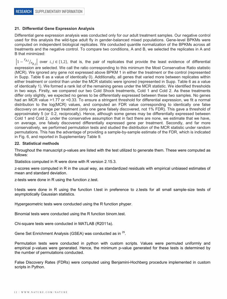
Finally we reviewed and recovered any missed known genes or transcripts in order to generate a comprehensive genome annotation. We reviewed our previous genome annotation efforts, which we now call modENCODE version 1 (MDv1) 3 and MDv214,15 to identify any gene or transcript models that were not reproduced in our GRIT and manual analysis. We also compared to FB5.45 and RefSeq (downloaded Feb. 2, 2013). This resulted in adding back a number of missed low expression genes as well as small RNA genes (e.g. tRNAs, miRNAs, etc.). These results are summarized in Supplementary Figure 1. The resulting complete annotation is MDv3 (Supplementary Data File 1), and includes attributions for each annotation.
14. Predicting proteins based on transcript models In each transcript, we automatically annotated the longest ORF as a predicted protein whenever that ORF was at least 100 aa in length. When the longest ORF was between 20 aa and 100 aa, we evaluated each ORF longer than 20 aa as follows: we ran RPS-BLAST using the CDD (as below) and annotated any ORF with a CDD hit E-value of 1e-5 or less; we ran PhyloCSF (as below) and annotated any ORF with a conservation score of -0.2 or more. We note that this procedure identified novel conserved ORFs in 277 FB5.45 “non-coding” genes out of 893 such annotated genes, as well as 391 conserved ORFs in novel genes. In all, short conserved ORFs were identified in 27% of genes with no ORF over 100aa. Only 5% of these calls were due to

SUPPLEMENTARY INFORMATION
1 0 | W W W. N A T U R E . C O M / N A T U R E
RESEARCH
the CDD RPS-BLAST search, the remainders were called by PhyloCSF. We consider these novel short ORFs “provisional”; extensive validation will be required to determine if they are translated in vivo.
15. siRNA analysis The Drosophila melanogaster genome was segmented based on small RNA-seq read coverage of small RNA libraries in heads (accession: GSM609251, GSM239041, GSM278704, GSM322533, GSM322543), ovaries (accession: GSM548586, GSM548585, GSM548583, GSM548592, GSM280086, GSM767595, GSM767594), and testes (accession: GSM909277, GSM909278, GSM548591, GSM548589, GSM548584, GSM548582). We clustered overlapping read regions into consensus segments and adjacent segments separated by less than 500 bp were then merged. The segments overlapping with TEs were excluded. cis-NAT siRNA features were extracted from these segments. Features used for the predictive model included 21 nt read frequency (21nt reads/all size reads); strand ratio (21 nt read ratio of sense/antisense); and read length distribution (mean, standard deviation, mode). We built a one-class predictive model which was trained on the previously published cisNAT siRNA loci from our and other labs16,17,18,19 using the above features, and was applied to predict cis-NAT siRNAs on all segments genome-wide, separately for each library. In summary, minimum expression for annotating cis-NAT siRNA loci were 21nt reads ≥ 1 RPM for both sense and antisense strands (5-95 percentile range is 2.9 – 70.4 RPM); minimum 21nt percentage (21nt reads/all size reads) for the calling siRNA loci was 60% (5-95 percentile range is 68% – 88%); minimum sense and antisense strand ratio was < 4.5 fold (5-95 percentile range is < 2.3 fold).
16. Identifying Conserved Domains in predicted proteins We utilized the NCBI Conserve Domain Database (CDD)20 and the Reverse Psi-BLAST (RPS-BLAST) tool21 to identify functional domains in predicted proteins, using default settings. We used an E-value threshold of 1e-5 to specify potential hits. The precise executable and settings utilized are detailed below:
# blast standalone execuatable (including RPS-BLAST algorithm): ftp://ftp.ncbi.nih.gov/blast/executables/release/2.2.26/blast-2.2.26-x64-linux.tar.gz # Conserved Domain detailed definitions and shortnames: ftp://ftp.ncbi.nih.gov/pub/mmdb/cdd/cddid_all.tbl.gz: # Binary Conserved Domain Database (downloaded 9/1/12): ftp://ftp.ncbi.nih.gov/pub/mmdb/cdd/big_endian/Cdd_BE.tar.gz The Reverse Position Specific BLAST 2.2.26+ algorithm as part of the NCBI BLAST+ standalone package (version 2.2.26) was used to identify conserved domains within putative conserved domains.
16A. Conserved Domain and GO analysis of complex loci To further characterize genes that express alternatively spliced transcripts, we examined conserved protein
domains. Among genes with the capacity to produce more than 100 transcripts (292 genes), there are a number of significantly enriched conserved protein domains (FDR<1%), several corresponding to RNA binding domains: K homology, ELAV/HuD family splicing factor, sex-lethal family splicing factor, glycine-rich RNA-binding protein 4 motif, heterogeneous nuclear ribonucleoprotein R, Q family, and the half-pint family. A number of kinase-related domains are also strongly enriched (Supplementary Table 5). The most enriched Biological Process GO term is synaptic transmission (16 genes, FDR<7e-14).
17. Identifying conserved ORFs that lack known domains We utilized the program PhyloCSF22 to identify novel conserved ORFs that lacked known domains in the CDD database. The inputs to the algorithm are the 14 flies multiple alignment in MAF format (reviewed in23) and the set of ORFs called by GRIT in our transcript annotation (see below, “Predicting proteins based on transcript models”). The algorithm was run as follows:
# PhyloCSF executable (as of 2012-10-28): http://github.com/mlin/PhyloCSF/tarball/20121028-exe PhlyoCSF is run in the "AsIs" mode which analyzes only the input ORFs (ORFs are not discovered by PhyloCSF). Based on communication with the Kellis group and their previous experience24 (also, personal communication with Mike Lin), we utilized a conservation score threshold of -0.2 to identify conserved proteins.

W W W. N A T U R E . C O M / N A T U R E | 1 1
SUPPLEMENTARY INFORMATION RESEARCH
18. Defining lncRNA elements We defined lncRNA genes as those that lack any coding transcript given the above definition, and that encode no known small RNA (e.g. tRNAs, miRNAs, etc.). We note that this means that our annotation includes non-coding transcripts of coding genes. In Drosophila, there is one gene known to encode four 11aa ORFs25, and hence it is possible that some of our lncRNAs may yet encode conserved and/or functional short polypeptides. However, PhyloCSF run time is exponential in minimum ORF length between 10 aa and 20 aa, due to an exponential increase in the number of such ORFs present in transcript models. Furthermore, the power of the model is predicated on being able to observe protein-coding structure in multi-species alignments, e.g. third base wobble22. This power is dampened in short ORFs, and after extensive manual review we determined that 20 aa was likely close to the limit of detection of the algorithm. This corresponds roughly to the limits of detection of MS/MS in our experience26, and highlights the difficulty of identifying short protein coding sequencing, and the importance of emerging assays such as Ribo-seq27.
19. MISO analysis of splicing dynamics We parsed the annotation gtf file to generate GFF3 files containing individual splicing event annotations using a perl script described14. MISO28 was used to quantitate the splicing events for all samples in single read mode as described in14.
We identified 25,756 alternative splicing events in the transcript models. Of these, we focused on 17,447 events that produce only two isoforms per gene and do not have overlapping annotated features that might confound quantitation and analysis. We calculated Ψ values for each event in each tissue and developmental sample. We observed nearly identical distributions of median Ψ values for all events across all samples, among just the developmental samples and among just the tissue samples (Supplementary Fig. 4). It has previously been shown that mammalian alternative exons whose magnitudes of splicing changes are large are more conserved and more frame-preserving than exons with low magnitude splicing changes30. To determine if this is also true in Drosophila, we characterized the conservation and reading-frame-preservation properties of cassette exons based on the magnitude of their tissue-specific regulation. We divided exons into three bins based on ∆Ψ: high (∆Ψ>50%, n=395), moderate (∆Ψ 25-50%, n=98) and low (∆Ψ<25%, n=68). Exons with high ∆Ψ are more conserved than those with moderate or low ∆Ψs, both within the exon and the flanking introns, in particular the upstream intron (Supplementary Fig. 11). In addition, we find that exons with high ∆Ψs tend to preserve the reading-frame more often than exons with moderate or low ∆Ψs (Supplementary Fig 10, chi-square p-value 1e-9, permutation test p-value 3e-8). 19A. Detailed analysis of sex-specific splicing in somatic tissues We previously identified hundreds of sex-specific splicing events from whole adult male and female RNA-seq data6. To further explore sex-specific splicing, we compared the splicing patterns in male and female heads. There were striking differences in gene expression levels between male and female heads, however, only six splicing events were consistently differentially spliced between males and females in heads at each time point after eclosion (average ∆Ψ>20%). Of these, the strongest was the sex-specific 5’ splice site in fruitless (avg. ∆Ψ=91%). Two other sex-specific splicing events occur in doublesex. The final three events were a retained intron in CG6236, an alternative 5’ splice site in Ca2+-channel protein α1 subunit T and an alternative first exon in Septin 4. Of the other known splicing events in the sex-determination pathway, the 5’ splice site in transformer had an average ∆Ψ of 48% (though one comparison had a ∆Ψ=16%), sex-specific splicing of male specific lethal-2 was not observed between male and female heads (avg. ∆Ψ=5%), and splicing events from Sex lethal (Sxl) were not quantified due to annotation complexity. When we conducted the quantification on a simplified set of transcripts (MDv13), Sxl is the most sex-specific splicing event in the genome. Surprisingly, these results show that there is little sex-specific splicing in Drosophila heads.
20. Computing gene expression Gene level expression measurements (Supplementary Data File 9) were computed in BPKM as previously described3 over the projected gene model. The projected gene models were determined by projecting all overlapping exons for each gene down into non-overlapping exon regions, and then computing the BPKM across the entire region.
SUPPLEMENTARY INFORMATION
1 2 | W W W. N A T U R E . C O M / N A T U R E
RESEARCH
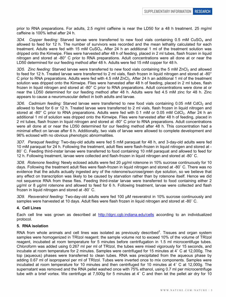
21. Differential Gene Expression Analysis Differential gene expression analysis was conducted only for our adult treatment samples. Our negative control used for this analysis the wild-type adult fly in gender-balanced mixed populations. Gene-level BPKMs were computed on independent biological replicates. We conducted quantile normalization of the BPKMs across all treatments and the negative control. To compare two conditions, A and B, we selected the replicates in A and B that minimized:
�1 − 𝑟𝑟𝐴𝐴,𝑖𝑖 𝑟𝑟𝐵𝐵,𝑗𝑗� � over 𝑖𝑖, 𝑗𝑗 ∈ {1,2}, that is, the pair of replicates that provide the least evidence of differential expression are selected. We call the ratio corresponding to this minimum the Most Conservative Ratio statistic (MCR). We ignored any gene not expressed above BPKM 1 in either the treatment or the control (represented in Supp. Table 6 as a value of identically 0). Additionally, all genes that varied more between replicates within either treatment or control than under the MCR statistic were ignored (represented in Supp. Table 6 as a value of identically 1). We formed a rank list of the remaining genes under the MCR statistic. We identified thresholds in two ways. Firstly, we compared our two Cold Shock treatments, Cold 1 and Cold 2. As these treatments differ only slightly, we expected no genes to be differentially expressed between these two samples. No genes had an MCR value >1.77 or <0.33. To ensure a stringent threshold for differential expression, we fit a normal distribution to the log(MCR) values, and computed an FDR value corresponding to identically one false discovery on average per treatment (only one gene falsely discovered, not 1% FDR). This gave a threshold of approximately 5 (or 0.2, reciprocally). Hence, although some genes may be differentially expressed between Cold 1 and Cold 2, under the conservative assumption that in fact there are none, we estimate that we have, on average, one falsely discovered differentially expressed gene per treatment. Secondly, and far more conservatively, we performed permutation tests and studied the distribution of the MCR statistic under random permutations. This has the advantage of providing a sample-by-sample estimate of the FDR, which is indicated in Fig. 6, and reported in Supplementary Table 9.
22. Statistical methods Throughout the manuscript p-values are listed with the test utilized to generate them. These were computed as follows:
Statistics computed in R were done with R version 2.15.3.
z-scores were computed in R in the usual way, as standardized residuals with empirical unbiased estimates of mean and standard deviation.
z-tests were done in R using the function z.test.
t-tests were done in R using the function t.test in preference to z.tests for all small sample-size tests of asymptotically Gaussian statistics.
Hypergeometric tests were conducted using the R function phyper.
Binomial tests were conducted using the R function binom.test.
Chi-square tests were conducted in MATLAB (R2011a).
Gene Set Enrichment Analysis (GSEA) was conducted as in 29.
Permutation tests were conducted in python with custom scripts. Values were permuted uniformly and empirical p-values were generated. Hence, the minimum p-value generated for these tests is determined by the number of permutations conducted.
False Discovery Rates (FDRs) were computed using Benjamini-Hochberg procedure implemented in custom scripts in Python.

W W W. N A T U R E . C O M / N A T U R E | 1 3
SUPPLEMENTARY INFORMATION RESEARCH
23. Supplementary Table Legends Supplementary Table 1: Comparison of recent annotations of the Drosophila melanogaster genome. Supplementary Table 2: Newly annotated genes overlapping molecularly defined mutations in the fly genome with associated phenotypes in the animal Supplementary Table 3: Counts of Introns, Transcripts, and Proteins per gene, for each gene in MDv3. Supplementary Table 4: In situ images and related data for 47 genes with the potential to produce more than 1000 transcript isoforms each. Supplementary Table 5: Enriched Conserved Domains and GO terms for genes with 100 or more transcript models Supplementary Table 6: Enriched Reactome Pathways for differentially genes with sex-specific splicing in somatic tissues. Supplementary Table 7: PhyloCSF scores for all ORFs between 20aa and 100aa in length Supplementary Table 8: Loci with antisense transcript models and siRNA expression along with associated expression scores in small RNA sequencing Supplementary Table 9: Gene induction/repression levels (and FDR) for treatments compared to negative control Supplementary Table 10: Production summary. All RNA sample names, assays, accession numbers, and read counts.
24. Supplementary Data Files Supplementary Data File 1: The annotation MDv3 in GTF file format Supplementary Data File 2: MDv3 models for candidate lncRNA genes in GTF format. This is a subset of Supplementary Data File 1. Supplementary Data File 3: Covariates used in the Random Forests prediction of bona fide polyadenylation sites. These are the covariates used to produce Supplementary Data File 4. Supplementary Data File 4: The Celniker cDNAs used in the Random Forest prediction of bona fide transcript start sites. Supplementary Data File 5: Genome-wide polyadenylation site annotation in bedGraph format. Supplementary Data File 6: GRIT configuration file. This file is provides the input to GRIT, precisely as it was run to produce the GRIT transcript models analyzed here.
Supplementary Data File 7: Filtered CAGE bedGraphs. These are the output of the Random Forests model, and should be regarded as “called peaks” in the CAGE data, or bona fide transcript start sites along with associated CAGE read counts.
Supplementary Data File 8: Covariates used in the Random Forests prediction of bona fide transcript start sites. These are the covariates used to produce Supplementary Data File 8.
Supplementary Data File 9: Gene expression scores in BPKM, comma delimited for the genes analyzed here, in MDv3. Annotation is given in Supplementary Data File 1.

SUPPLEMENTARY INFORMATION
1 4 | W W W. N A T U R E . C O M / N A T U R E
RESEARCH
25. Supplementary References 1 Celniker, S.E., et al. Finishing a whole-genome shotgun: Release 3 of the Drosophila melanogaster
euchromatic genome sequence. Genome Biology. 3(12)1-14. (2002) 2 Maroni G, Stamey SC. Use of blue food to select synchronous late third-instar larvae. Drosophila Inf
Serv. 59:142-143. (1983) 3 Graveley, B. R. et al. The developmental transcriptome of Drosophila melanogaster. Nature 471, 473-
479, doi:nature09715 [pii] 4 Functional Implications of the Unusual Spatial Distribution of a Minor a-Tubulin lsotype in Drosophila: A
Common Thread among Chordotonal Ligaments, Developing Muscle, and Testis Cyst Cells Kathleen A. Matthews, David F. B. Miller, and Thomas C. Kaufman. Developmental Biology 1990, 137, 171-183.
5 Fristrom JW, Mitchell HK. The preparative isolation of imaginal discs from larvae of Drosophila melanogaster. J Cell Biol. 27(2):445-8. (1965)
6 Smibert, P. et al. Global patterns of tissue-specific alternative polyadenylation in Drosophila. Cell Rep 1, 277-289, doi:10.1016/j.celrep.2012.01.001 (2012).
7 Djebali, S. et al. Landscape of transcription in human cells. Nature 489, 101-108, doi:nature11233 8 Takahashi, H., Lassmann, T., Murata, M. & Carninci, P. 5' end-centered expression profiling using cap-
analysis gene expression and next-generation sequencing. Nat Protoc 7, 542-561, doi:nprot.2012.005 [pii]
9 Hoskins, R. A. et al. Genome-wide analysis of promoter architecture in Drosophila melanogaster. Genome Res 21, 182-192, doi:gr.112466.110 [pii]
10 Wan, K. H. et al. High-throughput plasmid cDNA library screening. Nat Protoc 1, 624-632 (2006). 11 Boley, N., et al. Ab initio transcript assembly using gene boundary data. Submitted to Nature Biotech.
(2013) 12 Retelska, D., Iseli, C., Bucher, P., Jongeneel, C. V. & Naef, F. Similarities and differences of
polyadenylation signals in human and fly. BMC Genomics 7, 176, doi:1471-2164-7-176 [pii] 13 Bailey, T. L. et al. MEME SUITE: tools for motif discovery and searching. Nucleic Acids Res 37, W202-
208, doi:gkp335 [pii] 14 Gerstein, M. et al. Comparison of the transcriptomes of flies, human and worms. Nature. Submission
ID: 2012-12-15978A. (2013). 15 Oliver, B. Comparative trancriptome analysis using 20 Fly Species. Manuscript in preparation. (2013). 16 Okamura, K. & Lai, E.C. Endogenous small interfering RNAs in animals. Nat Rev Mol Cell Biol 9, 673-8
(2008). 17 Okamura, K., Balla, S., Martin, R., Liu, N. & Lai, E.C. Two distinct mechanisms generate endogenous
siRNAs from bidirectional transcription in Drosophila. Nat Struct Mol Biol 15, 581-590 (2008). 18 Czech, B. et al. An endogenous siRNA pathway in Drosophila. Nature 453, 798-802 (2008). 19 Ghildiyal, M. et al. Endogenous siRNAs Derived from Transposons and mRNAs in Drosophila Somatic
Cells. Science 320, 1077-1081 (2008). 20 Marchler-Bauer, A. et al. CDD: conserved domains and protein three-dimensional structure. Nucleic
Acids Res 41, D348-352, doi:gks1243 [pii] 21 Marchler-Bauer, A. & Bryant, S. H. CD-Search: protein domain annotations on the fly. Nucleic Acids
Res 32, W327-331, doi:10.1093/nar/gkh454 22 Lin, M. F., Jungreis, I. & Kellis, M. PhyloCSF: a comparative genomics method to distinguish protein
coding and non-coding regions. Bioinformatics 27, i275-282, doi:btr209 [pii]

W W W. N A T U R E . C O M / N A T U R E | 1 5
SUPPLEMENTARY INFORMATION RESEARCH
23 Blankenberg, D., Taylor, J. & Nekrutenko, A. Making whole genome multiple alignments usable for biologists. Bioinformatics 27, 2426-2428, doi:btr398 [pii]
24 Stark, A. et al. Discovery of functional elements in 12 Drosophila genomes using evolutionary signatures. Nature 450, 219-232, doi:nature06340 [pii]
25 Kondo, T. et al. Small peptide regulators of actin-based cell morphogenesis encoded by a polycistronic mRNA. Nat Cell Biol 9, 660-665, doi:ncb1595 [pii]
26 Banfai, B. et al. Long noncoding RNAs are rarely translated in two human cell lines. Genome Res 22, 1646-1657, doi:22/9/1646 [pii]
27 Ingolia, N. T., Ghaemmaghami, S., Newman, J. R. & Weissman, J. S. Genome-wide analysis in vivo of translation with nucleotide resolution using ribosome profiling. Science 324, 218-223, doi:1168978
28 Katz Y., Wang E.T., Airoldi E.M., Burge C.B. Analysis and design of RNA sequencing experiments for identifying isoform regulation.Nat Methods. 7(12):1009-15. doi: 10.1038/nmeth.1528. (2010)
29 Subramanian A., Tamayo P., Mootha V.K., Mukherjee S., Ebert B.L., Gillette M.A., Paulovich A., Pomeroy S.L., Golub T.R., Lander E.S. et al. Gene set enrichment analysis: a knowledge-based approach for interpreting genome-wide expression profiles. PNAS 102 15545–15550. (doi:10.1073/pnas.0506580102) (2005)
30 Wang, E. T. et al. Alternative isoform regulation in human tissue transcriptomes. Nature 456, 470-476, (2008).
SUPPLEMENTARY INFORMATION
1 6 | W W W. N A T U R E . C O M / N A T U R E
RESEARCH
0 10 25 50 75 90 1000
0.05
0.1
0.15
0.2
0.25
Known GenesNew Genes
% of samples above 1 BPKM
Frac
tion
of g
enes
Supplementary Figure 1 Summary of Annotation pie charts. Our annotation is primarily composed by models that were built by our automated pipeline, GRIT. To generate a comprehensive annotation of the Drosophila melanogaster genome, we additionally utilized previous community annotations (13%, FlyBase and RefSeq), including our own (5%), and limited manual re-annotation (4%).
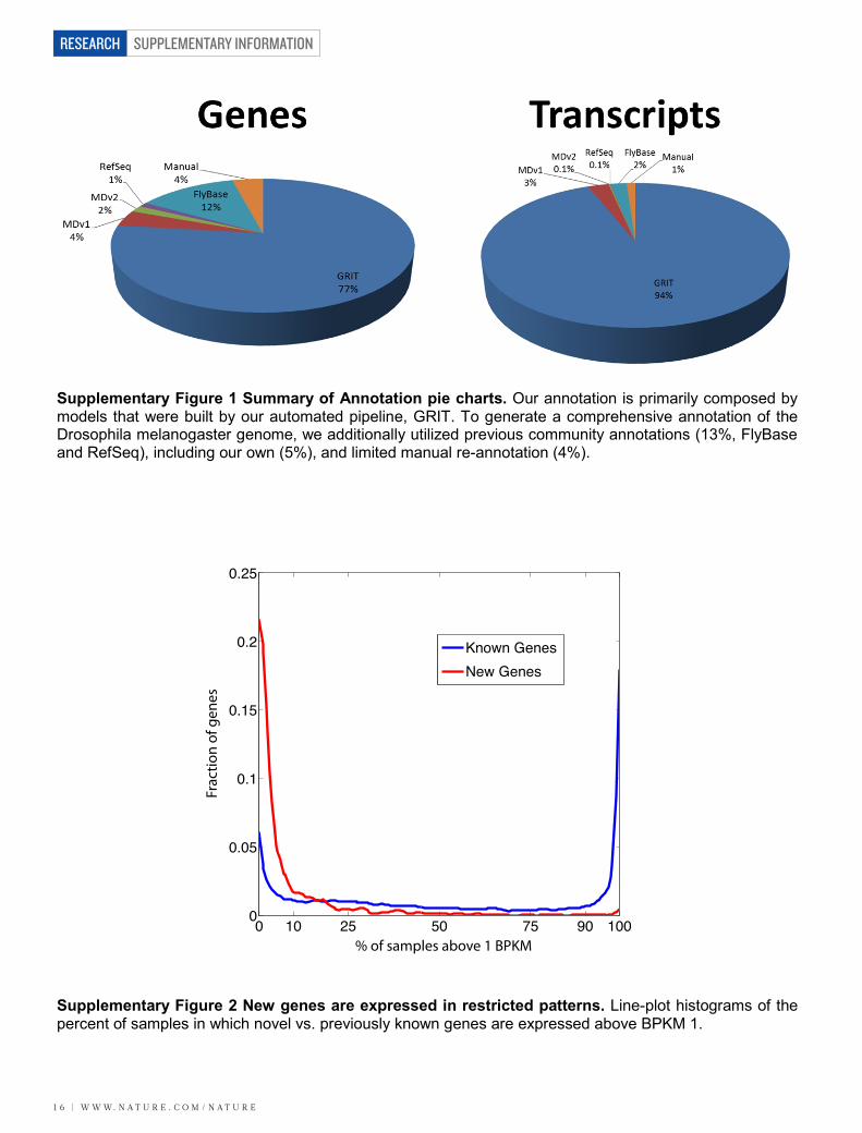
Supplementary Figure 2 New genes are expressed in restricted patterns. Line-plot histograms of the percent of samples in which novel vs. previously known genes are expressed above BPKM 1.
Supplementary Figure 3 Comparing splicing complexity in CDS sequence to that fund in UTRs and conservation of intron counts over Drosophilids. a, Complex processing and splicing of the 5’ UTR of Gβ13F. At the top of the figure are the testes and CNS positively stranded RNA-seq reads followed by the splice junctions (shaded gray as a function of usage), a simplified version of the full-length gene model and an expansion of the 5’ UTR showing some of the complexity. Transcription of the gene initiates from one of three different promoters (green arrows) terminates at one of ten possible polyA+ addition sites and via complex splicing patterns generates 235 transcripts that all produce the same protein. The first exon has two alternative splice acceptors that splice to one of eleven different donor sites. Only five donor sites are shown due to the proximity of the possible splice sites. Four splice donors are represented by the single red line and map to positions 15,755,148, 67, 72, 84 differing by 12, 5 and 19 bp respectively. Three splice donors are represented by the single green line and map to positions 15,755,256, 68, 79 differing by 12 and 11 bp. Two splice donors are represented by the single purple line 15,755, 409, 16 differing by 7 bp. These splice variants are combined with four different proximal internal splice junctions to generate the full complement of transcripts. Polyadenylation site, shown in red, come from Polya-seq of adult heads. b, scatter plot (as heat map) of the number of possible 5’UTR configurations vs. the number of possible CDS configurations for each gene, shown in log2 scale. c, A box plot of the number of configurations of 5’UTRs, 3’UTRs and CDS in which each intron participates. d, Histogram of splice-forms per gene for protein-coding genes (PCGs) for 5'UTRs, CDS, and 3'UTRs. e, Intron counts are conserved between drosophilids15. Indicated are two outliers that have undergone species-specific expansion. We attribute the fact that we observe more outliers in the melanogaster lineage to the superior quality of the assembled genome and the increased depth of sequencing data.
Supplementary Figure 4 Line-plot histograms of Ψ and ∆Ψ values for various classes of splicing events. Comparing all samples to Developmental and Tissue (Organ System) samples analyzed independently.
Supplementary Figure 5 Examples of genomic regions with sense/antisense transcription. Six genomic regions are highlighted. In regions where short RNA signal is not shown, short RNA sequencing does not reveal substantial siRNA (i.e. 21 nt-dominant small RNA) signal.
Supplementary Figure 6 lncRNA/mRNA sense-antisense pairs are more positively correlated than mRNA/mRNA sense-antisense pairs. a, QQ-plot of empirical distribution of pearson correlations between non-coding / coding antisense pairs vs. coding / coding antisense pairs. b, as in 5a, but restricted to cell line samples, where unexpressed lncRNAs pairs are given a r value of zero.
Supplementary Figure 7 Distribution of cis-NAT siRNA loci across tissues. a, Number of cis-NAT siRNA loci overlapped with antisense transcripts in testis, ovary, head small RNA-seq libraries, separately for tissue-specific cis-NAT siRNA, and those found in two or more tissues. Testis-specific siRNA loci show strong enrichment compared to head and ovary. b, Expression of tissue-specific cis-NAT siRNA loci overlapped with antisense transcripts also show strong enrichment in testes compared to head and ovary. Expression defined as average 21nt reads (RPM) of the libraries in a particular tissue, excluding outlier libraries that have < 100 21nt reads overlapping cis-NAT siRNA loci to increase robustness against low
Supplementary Figure 1 Summary of Annotation pie charts. Our annotation is primarily composed by models that were built by our automated pipeline, GRIT. To generate a comprehensive annotation of the Drosophila melanogaster genome, we additionally utilized previous community annotations (13%, FlyBase and RefSeq), including our own (5%), and limited manual re-annotation (4%).
Supplementary Figure 2 New genes are expressed in restricted patterns. Line-plot histograms of the percent of samples in which novel vs. previously known genes are expressed above BPKM 1.
Supplementary Figure 3 Comparing splicing complexity in CDS sequence to that fund in UTRs and conservation of intron counts over Drosophilids. a, Complex processing and splicing of the 5’ UTR of Gβ13F. At the top of the figure are the testes and CNS positively stranded RNA-seq reads followed by the splice junctions (shaded gray as a function of usage), a simplified version of the full-length gene model and an expansion of the 5’ UTR showing some of the complexity. Transcription of the gene initiates from one of three different promoters (green arrows) terminates at one of ten possible polyA+ addition sites and via complex splicing patterns generates 235 transcripts that all produce the same protein. The first exon has two alternative splice acceptors that splice to one of eleven different donor sites. Only five donor sites are shown due to the proximity of the possible splice sites. Four splice donors are represented by the single red line and map to positions 15,755,148, 67, 72, 84 differing by 12, 5 and 19 bp respectively. Three splice donors are represented by the single green line and map to positions 15,755,256, 68, 79 differing by 12 and 11 bp. Two splice donors are represented by the single purple line 15,755, 409, 16 differing by 7 bp. These splice variants are combined with four different proximal internal splice junctions to generate the full complement of transcripts. Polyadenylation site, shown in red, come from Polya-seq of adult heads. b, scatter plot (as heat map) of the number of possible 5’UTR configurations vs. the number of possible CDS configurations for each gene, shown in log2 scale. c, A box plot of the number of configurations of 5’UTRs, 3’UTRs and CDS in which each intron participates. d, Histogram of splice-forms per gene for protein-coding genes (PCGs) for 5'UTRs, CDS, and 3'UTRs. e, Intron counts are conserved between drosophilids15. Indicated are two outliers that have undergone species-specific expansion. We attribute the fact that we observe more outliers in the melanogaster lineage to the superior quality of the assembled genome and the increased depth of sequencing data.
Supplementary Figure 4 Line-plot histograms of Ψ and ∆Ψ values for various classes of splicing events. Comparing all samples to Developmental and Tissue (Organ System) samples analyzed independently.
Supplementary Figure 5 Examples of genomic regions with sense/antisense transcription. Six genomic regions are highlighted. In regions where short RNA signal is not shown, short RNA sequencing does not reveal substantial siRNA (i.e. 21 nt-dominant small RNA) signal.
Supplementary Figure 6 lncRNA/mRNA sense-antisense pairs are more positively correlated than mRNA/mRNA sense-antisense pairs. a, QQ-plot of empirical distribution of pearson correlations between non-coding / coding antisense pairs vs. coding / coding antisense pairs. b, as in 5a, but restricted to cell line samples, where unexpressed lncRNAs pairs are given a r value of zero.
Supplementary Figure 7 Distribution of cis-NAT siRNA loci across tissues. a, Number of cis-NAT siRNA loci overlapped with antisense transcripts in testis, ovary, head small RNA-seq libraries, separately for tissue-specific cis-NAT siRNA, and those found in two or more tissues. Testis-specific siRNA loci show strong enrichment compared to head and ovary. b, Expression of tissue-specific cis-NAT siRNA loci overlapped with antisense transcripts also show strong enrichment in testes compared to head and ovary. Expression defined as average 21nt reads (RPM) of the libraries in a particular tissue, excluding outlier libraries that have < 100 21nt reads overlapping cis-NAT siRNA loci to increase robustness against low

W W W. N A T U R E . C O M / N A T U R E | 1 7
SUPPLEMENTARY INFORMATION RESEARCH
b
a
No.
of t
rans
incl
udin
g ea
ch in
tron
5UTR CDS 3UTR0
1
2
3
4
5
6
7
8
0.3 1 3 10
0.1
0.3
1
3
10
5’UTRs isoforms per intron
CDS
isof
orm
s pe
r int
ron
c
1 2-4 5-9 >100
0.2
0.4
0.6
0.8
15’UTRCDS3’UTR
Splicing events per gene
Frac
tion
of P
CGs
d
Splice junctions per gene (D. melanogaster)
Splic
e ju
nctio
ns p
er g
ene
(D. p
seud
oobs
cura
)
0 10 20 30 40 50
05
1015
2025
30
4422251155830158421
mtd
heph●
●
●
●
●
●
●
●
●
●
●
●
●
●
●
●
●
●
●
●
●
●
●
●
●
●
●
●
●
●
●
●
●
●
●
●
●
●
●
●
●
●
●
●
●
●
●
●
●
●
●
●
●
●
●
●
●
●
●
●
●
●
●
●
●
●
●
●
●
●
●
●
●
●
●
●
●
●
●
●
●
●
●
●
●
●
●
●
●
●
●
●
●
●
●
●
●
●
●
●
●
●
●
●
●
●
●
●
●
●
●
●
●
●
●
●
●
●
●
●
●
●
●
●
●
●
●
●
●
●
●
●
●
●
●
●
●
●
●
●
●
●
●
●
●
●
●
●
●
●
●
●
●
●
●
●
●
●
●
●
●
●
●
●
●
●
●
●
●
●
●
●
●
●
●
●
●
●
●
●
●
●
●
●
●
●
●
●
●
●
●
●
●
●
●
●
●
●
●
●
●
●
●
●
●
●
●
●
●
●
●
●
●
●
●
●
●
●
●
●
●
●
●
●
●
●
●
●
●
●
●
●
●
●
●
●
●
●
●
●
●
●
●
●
●
●
●
●
●
●
●
●
●
●
●
●
●
●
●
●
●
●
●
●
●
●
●
●
●
●
AAAAAAAAAA
AAAAAAAAAAAAAAA
AAAAAAAAAA
AAAAA
AAAAAAAAAA
206 8622
361 9672
Junctions
Transcript Models
Tissue-SpecificRNA-Seq
Transcript Models
Expansion of the 5’ ends
chrX15,755K 15,756K 15,757K 15,758K 15,759K 15,760K
CNS
Testes
Gbeta13F
e
Supplementary Figure 1 Summary of Annotation pie charts. Our annotation is primarily composed by models that were built by our automated pipeline, GRIT. To generate a comprehensive annotation of the Drosophila melanogaster genome, we additionally utilized previous community annotations (13%, FlyBase and RefSeq), including our own (5%), and limited manual re-annotation (4%).
Supplementary Figure 2 New genes are expressed in restricted patterns. Line-plot histograms of the percent of samples in which novel vs. previously known genes are expressed above BPKM 1.
Supplementary Figure 3 Comparing splicing complexity in CDS sequence to that fund in UTRs and conservation of intron counts over Drosophilids. a, Complex processing and splicing of the 5’ UTR of Gβ13F. At the top of the figure are the testes and CNS positively stranded RNA-seq reads followed by the splice junctions (shaded gray as a function of usage), a simplified version of the full-length gene model and an expansion of the 5’ UTR showing some of the complexity. Transcription of the gene initiates from one of three different promoters (green arrows) terminates at one of ten possible polyA+ addition sites and via complex splicing patterns generates 235 transcripts that all produce the same protein. The first exon has two alternative splice acceptors that splice to one of eleven different donor sites. Only five donor sites are shown due to the proximity of the possible splice sites. Four splice donors are represented by the single red line and map to positions 15,755,148, 67, 72, 84 differing by 12, 5 and 19 bp respectively. Three splice donors are represented by the single green line and map to positions 15,755,256, 68, 79 differing by 12 and 11 bp. Two splice donors are represented by the single purple line 15,755, 409, 16 differing by 7 bp. These splice variants are combined with four different proximal internal splice junctions to generate the full complement of transcripts. Polyadenylation site, shown in red, come from Polya-seq of adult heads. b, scatter plot (as heat map) of the number of possible 5’UTR configurations vs. the number of possible CDS configurations for each gene, shown in log2 scale. c, A box plot of the number of configurations of 5’UTRs, 3’UTRs and CDS in which each intron participates. d, Histogram of splice-forms per gene for protein-coding genes (PCGs) for 5'UTRs, CDS, and 3'UTRs. e, Intron counts are conserved between drosophilids15. Indicated are two outliers that have undergone species-specific expansion. We attribute the fact that we observe more outliers in the melanogaster lineage to the superior quality of the assembled genome and the increased depth of sequencing data.
Supplementary Figure 4 Line-plot histograms of Ψ and ∆Ψ values for various classes of splicing events. Comparing all samples to Developmental and Tissue (Organ System) samples analyzed independently.
Supplementary Figure 5 Examples of genomic regions with sense/antisense transcription. Six genomic regions are highlighted. In regions where short RNA signal is not shown, short RNA sequencing does not reveal substantial siRNA (i.e. 21 nt-dominant small RNA) signal.
Supplementary Figure 6 lncRNA/mRNA sense-antisense pairs are more positively correlated than mRNA/mRNA sense-antisense pairs. a, QQ-plot of empirical distribution of pearson correlations between non-coding / coding antisense pairs vs. coding / coding antisense pairs. b, as in 5a, but restricted to cell line samples, where unexpressed lncRNAs pairs are given a r value of zero.
Supplementary Figure 7 Distribution of cis-NAT siRNA loci across tissues. a, Number of cis-NAT siRNA loci overlapped with antisense transcripts in testis, ovary, head small RNA-seq libraries, separately for tissue-specific cis-NAT siRNA, and those found in two or more tissues. Testis-specific siRNA loci show strong enrichment compared to head and ovary. b, Expression of tissue-specific cis-NAT siRNA loci overlapped with antisense transcripts also show strong enrichment in testes compared to head and ovary. Expression defined as average 21nt reads (RPM) of the libraries in a particular tissue, excluding outlier libraries that have < 100 21nt reads overlapping cis-NAT siRNA loci to increase robustness against low

SUPPLEMENTARY INFORMATION
1 8 | W W W. N A T U R E . C O M / N A T U R E
RESEARCH
Supplementary Figure 1 Summary of Annotation pie charts. Our annotation is primarily composed by models that were built by our automated pipeline, GRIT. To generate a comprehensive annotation of the Drosophila melanogaster genome, we additionally utilized previous community annotations (13%, FlyBase and RefSeq), including our own (5%), and limited manual re-annotation (4%).
Supplementary Figure 2 New genes are expressed in restricted patterns. Line-plot histograms of the percent of samples in which novel vs. previously known genes are expressed above BPKM 1.
Supplementary Figure 3 Comparing splicing complexity in CDS sequence to that fund in UTRs and conservation of intron counts over Drosophilids. a, Complex processing and splicing of the 5’ UTR of Gβ13F. At the top of the figure are the testes and CNS positively stranded RNA-seq reads followed by the splice junctions (shaded gray as a function of usage), a simplified version of the full-length gene model and an expansion of the 5’ UTR showing some of the complexity. Transcription of the gene initiates from one of three different promoters (green arrows) terminates at one of ten possible polyA+ addition sites and via complex splicing patterns generates 235 transcripts that all produce the same protein. The first exon has two alternative splice acceptors that splice to one of eleven different donor sites. Only five donor sites are shown due to the proximity of the possible splice sites. Four splice donors are represented by the single red line and map to positions 15,755,148, 67, 72, 84 differing by 12, 5 and 19 bp respectively. Three splice donors are represented by the single green line and map to positions 15,755,256, 68, 79 differing by 12 and 11 bp. Two splice donors are represented by the single purple line 15,755, 409, 16 differing by 7 bp. These splice variants are combined with four different proximal internal splice junctions to generate the full complement of transcripts. Polyadenylation site, shown in red, come from Polya-seq of adult heads. b, scatter plot (as heat map) of the number of possible 5’UTR configurations vs. the number of possible CDS configurations for each gene, shown in log2 scale. c, A box plot of the number of configurations of 5’UTRs, 3’UTRs and CDS in which each intron participates. d, Histogram of splice-forms per gene for protein-coding genes (PCGs) for 5'UTRs, CDS, and 3'UTRs. e, Intron counts are conserved between drosophilids15. Indicated are two outliers that have undergone species-specific expansion. We attribute the fact that we observe more outliers in the melanogaster lineage to the superior quality of the assembled genome and the increased depth of sequencing data.
Supplementary Figure 4 Line-plot histograms of Ψ and ∆Ψ values for various classes of splicing events. Comparing all samples to Developmental and Tissue (Organ System) samples analyzed independently.
Supplementary Figure 5 Examples of genomic regions with sense/antisense transcription. Six genomic regions are highlighted. In regions where short RNA signal is not shown, short RNA sequencing does not reveal substantial siRNA (i.e. 21 nt-dominant small RNA) signal.
Supplementary Figure 6 lncRNA/mRNA sense-antisense pairs are more positively correlated than mRNA/mRNA sense-antisense pairs. a, QQ-plot of empirical distribution of pearson correlations between non-coding / coding antisense pairs vs. coding / coding antisense pairs. b, as in 5a, but restricted to cell line samples, where unexpressed lncRNAs pairs are given a r value of zero.
Supplementary Figure 7 Distribution of cis-NAT siRNA loci across tissues. a, Number of cis-NAT siRNA loci overlapped with antisense transcripts in testis, ovary, head small RNA-seq libraries, separately for tissue-specific cis-NAT siRNA, and those found in two or more tissues. Testis-specific siRNA loci show strong enrichment compared to head and ovary. b, Expression of tissue-specific cis-NAT siRNA loci overlapped with antisense transcripts also show strong enrichment in testes compared to head and ovary. Expression defined as average 21nt reads (RPM) of the libraries in a particular tissue, excluding outlier libraries that have < 100 21nt reads overlapping cis-NAT siRNA loci to increase robustness against low
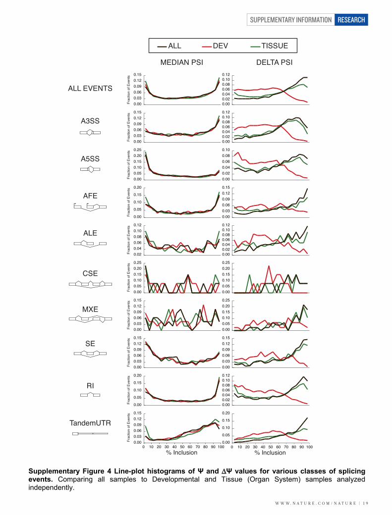
W W W. N A T U R E . C O M / N A T U R E | 1 9
SUPPLEMENTARY INFORMATION RESEARCH
0.000.030.060.090.120.15
TISSUEDEV
MEDIAN PSI DELTA PSI
ALL
0.000.020.040.060.080.100.12
ALL EVENTS
Frac
tion
of E
vent
sFr
actio
n of
Eve
nts
Frac
tion
of E
vent
sFr
actio
n of
Eve
nts
Frac
tion
of E
vent
sFr
actio
n of
Eve
nts
Frac
tion
of E
vent
sFr
actio
n of
Eve
nts
Frac
tion
of E
vent
sFr
actio
n of
Eve
nts
0.000.030.060.090.120.15
0.000.020.040.060.080.100.12
0.000.050.100.150.200.25
0.000.020.040.060.080.10
0.00
0.05
0.10
0.15
0.20
0.000.030.060.090.120.15
0.020.040.060.080.100.12
0.000.020.040.060.080.100.12
0.000.050.100.150.200.25
0.000.050.100.150.200.25
0.000.030.060.090.120.15
0.000.050.100.150.200.25
0.000.030.060.090.120.15
0.000.030.060.090.120.15
0.00
0.05
0.10
0.15
0.20
0.000.020.040.060.080.100.12
0.000.030.060.090.120.15
0.00
0.05
0.10
0.15
0.20
TandemUTR
RI
MXE
CSE
ALE
AFE
A3SS
A5SS
90 10080706050403020100% Inclusion
90 10080706050403020100% Inclusion
SE
Supplementary Figure 1 Summary of Annotation pie charts. Our annotation is primarily composed by models that were built by our automated pipeline, GRIT. To generate a comprehensive annotation of the Drosophila melanogaster genome, we additionally utilized previous community annotations (13%, FlyBase and RefSeq), including our own (5%), and limited manual re-annotation (4%).
Supplementary Figure 2 New genes are expressed in restricted patterns. Line-plot histograms of the percent of samples in which novel vs. previously known genes are expressed above BPKM 1.
Supplementary Figure 3 Comparing splicing complexity in CDS sequence to that fund in UTRs and conservation of intron counts over Drosophilids. a, Complex processing and splicing of the 5’ UTR of Gβ13F. At the top of the figure are the testes and CNS positively stranded RNA-seq reads followed by the splice junctions (shaded gray as a function of usage), a simplified version of the full-length gene model and an expansion of the 5’ UTR showing some of the complexity. Transcription of the gene initiates from one of three different promoters (green arrows) terminates at one of ten possible polyA+ addition sites and via complex splicing patterns generates 235 transcripts that all produce the same protein. The first exon has two alternative splice acceptors that splice to one of eleven different donor sites. Only five donor sites are shown due to the proximity of the possible splice sites. Four splice donors are represented by the single red line and map to positions 15,755,148, 67, 72, 84 differing by 12, 5 and 19 bp respectively. Three splice donors are represented by the single green line and map to positions 15,755,256, 68, 79 differing by 12 and 11 bp. Two splice donors are represented by the single purple line 15,755, 409, 16 differing by 7 bp. These splice variants are combined with four different proximal internal splice junctions to generate the full complement of transcripts. Polyadenylation site, shown in red, come from Polya-seq of adult heads. b, scatter plot (as heat map) of the number of possible 5’UTR configurations vs. the number of possible CDS configurations for each gene, shown in log2 scale. c, A box plot of the number of configurations of 5’UTRs, 3’UTRs and CDS in which each intron participates. d, Histogram of splice-forms per gene for protein-coding genes (PCGs) for 5'UTRs, CDS, and 3'UTRs. e, Intron counts are conserved between drosophilids15. Indicated are two outliers that have undergone species-specific expansion. We attribute the fact that we observe more outliers in the melanogaster lineage to the superior quality of the assembled genome and the increased depth of sequencing data.
Supplementary Figure 4 Line-plot histograms of Ψ and ∆Ψ values for various classes of splicing events. Comparing all samples to Developmental and Tissue (Organ System) samples analyzed independently.
Supplementary Figure 5 Examples of genomic regions with sense/antisense transcription. Six genomic regions are highlighted. In regions where short RNA signal is not shown, short RNA sequencing does not reveal substantial siRNA (i.e. 21 nt-dominant small RNA) signal.
Supplementary Figure 6 lncRNA/mRNA sense-antisense pairs are more positively correlated than mRNA/mRNA sense-antisense pairs. a, QQ-plot of empirical distribution of pearson correlations between non-coding / coding antisense pairs vs. coding / coding antisense pairs. b, as in 5a, but restricted to cell line samples, where unexpressed lncRNAs pairs are given a r value of zero.
Supplementary Figure 7 Distribution of cis-NAT siRNA loci across tissues. a, Number of cis-NAT siRNA loci overlapped with antisense transcripts in testis, ovary, head small RNA-seq libraries, separately for tissue-specific cis-NAT siRNA, and those found in two or more tissues. Testis-specific siRNA loci show strong enrichment compared to head and ovary. b, Expression of tissue-specific cis-NAT siRNA loci overlapped with antisense transcripts also show strong enrichment in testes compared to head and ovary. Expression defined as average 21nt reads (RPM) of the libraries in a particular tissue, excluding outlier libraries that have < 100 21nt reads overlapping cis-NAT siRNA loci to increase robustness against low

SUPPLEMENTARY INFORMATION
2 0 | W W W. N A T U R E . C O M / N A T U R E
RESEARCH
yellow-h
Mgn00290
Pgant35A
chr4 249K 249.5K 250K 250.5K 251K
144 _53 _
47 _
-391 _
Imaginal Disc +-
Testes +-
Gene Models
Tissue-SpecificRNA-Seq
prd
Mgn00375Mgn00376
12,083.5K 12,084K 12,084.5K 12,085K 12,085.5K 12,086K 12,086.5K 12,087K 12,087.5K
456 _
72 _
-456 _ 201 _
-17 _-1800 _
-1800 _
Conservation
Imaginal Disc +-
Testes +-
Gene Models
Tissue-SpecificRNA-Seq
Conservation
chr2L 14,359.5K 14,360K 14,360.5K 14,361K
CR43463
1568 _
1774 _
Testes +-
Lcch3
chrX 15,820K 15,821K 15,822K 15,823K 15,824K 15,825K
Ranbp16
-1077 _
417 _
890 _-72 _
Imaginal Disc +-
AdMF 1D Heads +-
248.5K
chr2L
chr2L 16,710K 16,715K
CG31782
CG31808
Cyt-c-d
16,705K
Gene Models
Tissue-SpecificRNA-Seq
Conservation
21nt Testes
-5 -397
4086 52,202
78
-45
21nt Testes
Testes +-
chr3L3,200K 3,205K 3,210K 3,215K
CG32276
gry
CG32271
CG33159 CG32277
CG33160CG32269CG32270
CG14967CG12034
454
-500
84
-2177
AdMF 1D Heads +-
21 nt AdMF 1D Heads +-
Supplementary Figure 1 Summary of Annotation pie charts. Our annotation is primarily composed by models that were built by our automated pipeline, GRIT. To generate a comprehensive annotation of the Drosophila melanogaster genome, we additionally utilized previous community annotations (13%, FlyBase and RefSeq), including our own (5%), and limited manual re-annotation (4%).
Supplementary Figure 2 New genes are expressed in restricted patterns. Line-plot histograms of the percent of samples in which novel vs. previously known genes are expressed above BPKM 1.
Supplementary Figure 3 Comparing splicing complexity in CDS sequence to that fund in UTRs and conservation of intron counts over Drosophilids. a, Complex processing and splicing of the 5’ UTR of Gβ13F. At the top of the figure are the testes and CNS positively stranded RNA-seq reads followed by the splice junctions (shaded gray as a function of usage), a simplified version of the full-length gene model and an expansion of the 5’ UTR showing some of the complexity. Transcription of the gene initiates from one of three different promoters (green arrows) terminates at one of ten possible polyA+ addition sites and via complex splicing patterns generates 235 transcripts that all produce the same protein. The first exon has two alternative splice acceptors that splice to one of eleven different donor sites. Only five donor sites are shown due to the proximity of the possible splice sites. Four splice donors are represented by the single red line and map to positions 15,755,148, 67, 72, 84 differing by 12, 5 and 19 bp respectively. Three splice donors are represented by the single green line and map to positions 15,755,256, 68, 79 differing by 12 and 11 bp. Two splice donors are represented by the single purple line 15,755, 409, 16 differing by 7 bp. These splice variants are combined with four different proximal internal splice junctions to generate the full complement of transcripts. Polyadenylation site, shown in red, come from Polya-seq of adult heads. b, scatter plot (as heat map) of the number of possible 5’UTR configurations vs. the number of possible CDS configurations for each gene, shown in log2 scale. c, A box plot of the number of configurations of 5’UTRs, 3’UTRs and CDS in which each intron participates. d, Histogram of splice-forms per gene for protein-coding genes (PCGs) for 5'UTRs, CDS, and 3'UTRs. e, Intron counts are conserved between drosophilids15. Indicated are two outliers that have undergone species-specific expansion. We attribute the fact that we observe more outliers in the melanogaster lineage to the superior quality of the assembled genome and the increased depth of sequencing data.
Supplementary Figure 4 Line-plot histograms of Ψ and ∆Ψ values for various classes of splicing events. Comparing all samples to Developmental and Tissue (Organ System) samples analyzed independently.
Supplementary Figure 5 Examples of genomic regions with sense/antisense transcription. Six genomic regions are highlighted. In regions where short RNA signal is not shown, short RNA sequencing does not reveal substantial siRNA (i.e. 21 nt-dominant small RNA) signal.
Supplementary Figure 6 lncRNA/mRNA sense-antisense pairs are more positively correlated than mRNA/mRNA sense-antisense pairs. a, QQ-plot of empirical distribution of pearson correlations between non-coding / coding antisense pairs vs. coding / coding antisense pairs. b, as in 5a, but restricted to cell line samples, where unexpressed lncRNAs pairs are given a r value of zero.
Supplementary Figure 7 Distribution of cis-NAT siRNA loci across tissues. a, Number of cis-NAT siRNA loci overlapped with antisense transcripts in testis, ovary, head small RNA-seq libraries, separately for tissue-specific cis-NAT siRNA, and those found in two or more tissues. Testis-specific siRNA loci show strong enrichment compared to head and ovary. b, Expression of tissue-specific cis-NAT siRNA loci overlapped with antisense transcripts also show strong enrichment in testes compared to head and ovary. Expression defined as average 21nt reads (RPM) of the libraries in a particular tissue, excluding outlier libraries that have < 100 21nt reads overlapping cis-NAT siRNA loci to increase robustness against low

W W W. N A T U R E . C O M / N A T U R E | 2 1
SUPPLEMENTARY INFORMATION RESEARCH
−0.4 −0.2 0 0.2 0.4 0.6 0.8 1−0.4
−0.2
0
0.2
0.4
0.6
0.8
1
Noncoding / Coding
Cod
ing
/ Cod
ing
QQ Plot of Pearson Correlation Noncoding/Coding vs. Coding/Coding Antisense Pairs
−0.5 0 0.5 1−0.5
0
0.5
1
Noncoding / Coding
Cod
ing
/ Cod
ing
QQ Plot of Pearson Correlation Noncoding/Coding vs. Coding/Coding Antisense PairsCell Lines Only
a.
b.
Supplementary Figure 1 Summary of Annotation pie charts. Our annotation is primarily composed by models that were built by our automated pipeline, GRIT. To generate a comprehensive annotation of the Drosophila melanogaster genome, we additionally utilized previous community annotations (13%, FlyBase and RefSeq), including our own (5%), and limited manual re-annotation (4%).
Supplementary Figure 2 New genes are expressed in restricted patterns. Line-plot histograms of the percent of samples in which novel vs. previously known genes are expressed above BPKM 1.
Supplementary Figure 3 Comparing splicing complexity in CDS sequence to that fund in UTRs and conservation of intron counts over Drosophilids. a, Complex processing and splicing of the 5’ UTR of Gβ13F. At the top of the figure are the testes and CNS positively stranded RNA-seq reads followed by the splice junctions (shaded gray as a function of usage), a simplified version of the full-length gene model and an expansion of the 5’ UTR showing some of the complexity. Transcription of the gene initiates from one of three different promoters (green arrows) terminates at one of ten possible polyA+ addition sites and via complex splicing patterns generates 235 transcripts that all produce the same protein. The first exon has two alternative splice acceptors that splice to one of eleven different donor sites. Only five donor sites are shown due to the proximity of the possible splice sites. Four splice donors are represented by the single red line and map to positions 15,755,148, 67, 72, 84 differing by 12, 5 and 19 bp respectively. Three splice donors are represented by the single green line and map to positions 15,755,256, 68, 79 differing by 12 and 11 bp. Two splice donors are represented by the single purple line 15,755, 409, 16 differing by 7 bp. These splice variants are combined with four different proximal internal splice junctions to generate the full complement of transcripts. Polyadenylation site, shown in red, come from Polya-seq of adult heads. b, scatter plot (as heat map) of the number of possible 5’UTR configurations vs. the number of possible CDS configurations for each gene, shown in log2 scale. c, A box plot of the number of configurations of 5’UTRs, 3’UTRs and CDS in which each intron participates. d, Histogram of splice-forms per gene for protein-coding genes (PCGs) for 5'UTRs, CDS, and 3'UTRs. e, Intron counts are conserved between drosophilids15. Indicated are two outliers that have undergone species-specific expansion. We attribute the fact that we observe more outliers in the melanogaster lineage to the superior quality of the assembled genome and the increased depth of sequencing data.
Supplementary Figure 4 Line-plot histograms of Ψ and ∆Ψ values for various classes of splicing events. Comparing all samples to Developmental and Tissue (Organ System) samples analyzed independently.
Supplementary Figure 5 Examples of genomic regions with sense/antisense transcription. Six genomic regions are highlighted. In regions where short RNA signal is not shown, short RNA sequencing does not reveal substantial siRNA (i.e. 21 nt-dominant small RNA) signal.
Supplementary Figure 6 lncRNA/mRNA sense-antisense pairs are more positively correlated than mRNA/mRNA sense-antisense pairs. a, QQ-plot of empirical distribution of pearson correlations between non-coding / coding antisense pairs vs. coding / coding antisense pairs. b, as in 5a, but restricted to cell line samples, where unexpressed lncRNAs pairs are given a r value of zero.
Supplementary Figure 7 Distribution of cis-NAT siRNA loci across tissues. a, Number of cis-NAT siRNA loci overlapped with antisense transcripts in testis, ovary, head small RNA-seq libraries, separately for tissue-specific cis-NAT siRNA, and those found in two or more tissues. Testis-specific siRNA loci show strong enrichment compared to head and ovary. b, Expression of tissue-specific cis-NAT siRNA loci overlapped with antisense transcripts also show strong enrichment in testes compared to head and ovary. Expression defined as average 21nt reads (RPM) of the libraries in a particular tissue, excluding outlier libraries that have < 100 21nt reads overlapping cis-NAT siRNA loci to increase robustness against low

SUPPLEMENTARY INFORMATION
2 2 | W W W. N A T U R E . C O M / N A T U R E
RESEARCH
tissue specific found in two or more tissues
#cis
−NAT
siR
NA
loci
ov
erla
pped
with
ant
isen
se tr
ansc
ripts
0
50
100
150
200
head ovary testes
P=2E-17P=4E-25
0
500
1000
1500
2000
2500
head ovary testes
tissu
e-sp
ecifi
c si
RN
A lo
ci21
nt m
ean
expr
essi
on (R
PM)
b
c
a
0.0
0.1
0.2
0.3
0.4
all samples
conditions
embryo development stages
tissues
Mea
n co
rrela
tion
coef
ficie
nt
produce cis−NAT siRNAsnot produce cis−NAT siRNAs
sense/antisense transcripts
Supplementary Figure 1 Summary of Annotation pie charts. Our annotation is primarily composed by models that were built by our automated pipeline, GRIT. To generate a comprehensive annotation of the Drosophila melanogaster genome, we additionally utilized previous community annotations (13%, FlyBase and RefSeq), including our own (5%), and limited manual re-annotation (4%).
Supplementary Figure 2 New genes are expressed in restricted patterns. Line-plot histograms of the percent of samples in which novel vs. previously known genes are expressed above BPKM 1.
Supplementary Figure 3 Comparing splicing complexity in CDS sequence to that fund in UTRs and conservation of intron counts over Drosophilids. a, Complex processing and splicing of the 5’ UTR of Gβ13F. At the top of the figure are the testes and CNS positively stranded RNA-seq reads followed by the splice junctions (shaded gray as a function of usage), a simplified version of the full-length gene model and an expansion of the 5’ UTR showing some of the complexity. Transcription of the gene initiates from one of three different promoters (green arrows) terminates at one of ten possible polyA+ addition sites and via complex splicing patterns generates 235 transcripts that all produce the same protein. The first exon has two alternative splice acceptors that splice to one of eleven different donor sites. Only five donor sites are shown due to the proximity of the possible splice sites. Four splice donors are represented by the single red line and map to positions 15,755,148, 67, 72, 84 differing by 12, 5 and 19 bp respectively. Three splice donors are represented by the single green line and map to positions 15,755,256, 68, 79 differing by 12 and 11 bp. Two splice donors are represented by the single purple line 15,755, 409, 16 differing by 7 bp. These splice variants are combined with four different proximal internal splice junctions to generate the full complement of transcripts. Polyadenylation site, shown in red, come from Polya-seq of adult heads. b, scatter plot (as heat map) of the number of possible 5’UTR configurations vs. the number of possible CDS configurations for each gene, shown in log2 scale. c, A box plot of the number of configurations of 5’UTRs, 3’UTRs and CDS in which each intron participates. d, Histogram of splice-forms per gene for protein-coding genes (PCGs) for 5'UTRs, CDS, and 3'UTRs. e, Intron counts are conserved between drosophilids15. Indicated are two outliers that have undergone species-specific expansion. We attribute the fact that we observe more outliers in the melanogaster lineage to the superior quality of the assembled genome and the increased depth of sequencing data.
Supplementary Figure 4 Line-plot histograms of Ψ and ∆Ψ values for various classes of splicing events. Comparing all samples to Developmental and Tissue (Organ System) samples analyzed independently.
Supplementary Figure 5 Examples of genomic regions with sense/antisense transcription. Six genomic regions are highlighted. In regions where short RNA signal is not shown, short RNA sequencing does not reveal substantial siRNA (i.e. 21 nt-dominant small RNA) signal.
Supplementary Figure 6 lncRNA/mRNA sense-antisense pairs are more positively correlated than mRNA/mRNA sense-antisense pairs. a, QQ-plot of empirical distribution of pearson correlations between non-coding / coding antisense pairs vs. coding / coding antisense pairs. b, as in 5a, but restricted to cell line samples, where unexpressed lncRNAs pairs are given a r value of zero.
Supplementary Figure 7 Distribution of cis-NAT siRNA loci across tissues. a, Number of cis-NAT siRNA loci overlapped with antisense transcripts in testis, ovary, head small RNA-seq libraries, separately for tissue-specific cis-NAT siRNA, and those found in two or more tissues. Testis-specific siRNA loci show strong enrichment compared to head and ovary. b, Expression of tissue-specific cis-NAT siRNA loci overlapped with antisense transcripts also show strong enrichment in testes compared to head and ovary. Expression defined as average 21nt reads (RPM) of the libraries in a particular tissue, excluding outlier libraries that have < 100 21nt reads overlapping cis-NAT siRNA loci to increase robustness against low read libraries down-weighting the average expression.
Supplementary Figure 8 Effects of environmental perturbations on the Drosophila transcriptome, full figure. Adults were treated with the stimulant, caffeine; heavy metals, Cd, Cu and Zn; temperature, cold and heat; and the herbicide, paraquat. a, A genome-wide map of genes that are up or down regulated as a function of Cd treatment. Labeled genes are those that showed a 20-fold (<10% FDR) change in response (linear scale). Genes highlighted in red are those identified previously in larvae50. In Fig. 6, some genes were omitted for readability. Those were: Jon25: Jon25Bi, Bii and Biii; Try: Trpα, β, γ, δ, ε, τ, CG30025 and CG30031; Acp53: Acp53C14a and b; Jon 65: Jon65Ai, iii, iv and yip7, Spn77: Spn77Bb, Spn77Bc; Hsp70: Hsp70Ab, Hsp70Aa, Hsp70Bb: Jon99C: Jon99Ci, Jon99ii; Jon99F: Jon99Fi and Jon99Fii; CG9468, CG7916, CG8997, CG17571, CG2065, CG18446, CG34054, CG42362, CG15126, CG13482, CG42363, CG43147, CG6295, CG10827, CG6125, CG16904 CG12057, CR40779 and CR40712. b, Heat map showing the fold change of genes with an FDR < 10% (of being differentially expressed) in at least one sample (log2 scale). c, Genes with the most enriched GO term “Response to Stimulus GO: 0050896”, hypergeometric FDR adjusted p-value < 1e-20 (log2 scale). d, Heat map showing the fold change of gonad-expressed genes encoding chorion (egg shell), yolk, seminal fluid, and male accessory gland proteins (log2 scale).
Supplementary Figure 9 Imaginal Disc mass isolation sample preparation. An image of the imaginal disc mass isolation sample preparation, along with anatomical annotations for the various
Supplementary Figure 10 Drosophila Body Map. An overview of the tissues collected in the adult and embryo dissections and mass tissue isolations. Maps between the larval progenitor tissues, which were isolated en masse in our sample enriched for Imaginal Discs, and connecting lines indicates corresponding adult tissues.
Supplementary Figure 11 Differential splicing in development and tissues. a, Fraction of splicing events with indicated ∆Ψ values amongst all developmental and tissue samples (black), between just developmental samples (red) and between just tissue samples (green). b, Conservation of cassette exons as a function of ∆Ψ values. c, Frame preservation of cassette exons as a function of ∆Ψ values.

W W W. N A T U R E . C O M / N A T U R E | 2 3
SUPPLEMENTARY INFORMATION RESEARCH
0 20 40 60 80 100 120 140 160−300
−200
−100
0
100
200
400
Jon25BiiiJon25BiiJon25Bi
Vm26Ab
CG7191
CG9468
Vm34Ca
CG8997CG7916
Lectin−galC1CG17571
Uhg3Gadd45CG2065
CG18446
thetaTry
alphaTry
epsilonTry
betaTrygammaTry
CG30031CG30025
deltaTry
CG34054
CG12374
Acp53C14aAcp53C14b
Amy−pAcp54A1
IM23
CG15126
Obp56g
CG42363CG42362
LysD
yip7Jon65AivJon65AiiiJon65Ai
Lcp65Ag2
Cp19
CR43482
CG18180
vsg
CG43147Acp70A
CG13482
Spn77BbSpn77Bc
7SLRNA
Fst
MtnA
CG16904
Hsp70AaHsp70Ab
GstD6
Hsp70Bb
CR44138
CG6125
MtnB
MtnD
CG10827CG6295
Jon99CiiJon99Ci
Anp
Jon99FiiJon99Fi
mt:ND1
CR40959 CR40779CR40712
Mgn570
Vml
Cp36
Cp38
CG12057
Mgn1457GstD2GstD5
2L 2R 3L 3R X
Cf 2.5m
gCf P
L
Cd 0.05
mM
Cd 0.1m
M
Cu 15m
M
Zn 4.5m
MCold
1Cold
2
Heat S
hock
PQ 5mM
PQ 10mM
Ge
ne
s (F
DR
10
%)
a
b c d
Treatments
Sfp35CAcp24A4Acp26AaSfp24Bb
Acp53C14aAcp53C14b
Acp53EaCp7Fa
Acp53C14cCp7FcSfp93FCp38Cp18
Sfp60FAcp63FAcp26AbAcp36DEAcp62FAcp76AAcp70ACp15Cp19
Sfp87BCp16Cp36Yp2
Acp54A1Acp98AB
Treatments
LysBLysDFst
14−3−3εHsp27
InRvsg
Rh6TequilaDopEcRCkIIbetaObp99bHsp67Bc
LysECecC
Hsp67BaHsp23
Hsp70BbbHsp70AaHsp70AbHsp67Bb
Hsp22Gγ1pucprosRdlgfA
Cyp6a2Cyp6a8
−5.0
−2.5
0.0
2.5
5.0
−7.5
−5.0
−2.5
0.0
−2.5
0.0
2.5
5.0
read libraries down-weighting the average expression.
Supplementary Figure 8 Effects of environmental perturbations on the Drosophila transcriptome, full figure. Adults were treated with the stimulant, caffeine; heavy metals, Cd, Cu and Zn; temperature, cold and heat; and the herbicide, paraquat. a, A genome-wide map of genes that are up or down regulated as a function of Cd treatment. Labeled genes are those that showed a 20-fold (<10% FDR) change in response (linear scale). Genes highlighted in red are those identified previously in larvae50. In Fig. 6, some genes were omitted for readability. Those were: Jon25: Jon25Bi, Bii and Biii; Try: Trpα, β, γ, δ, ε, τ, CG30025 and CG30031; Acp53: Acp53C14a and b; Jon 65: Jon65Ai, iii, iv and yip7, Spn77: Spn77Bb, Spn77Bc; Hsp70: Hsp70Ab, Hsp70Aa, Hsp70Bb: Jon99C: Jon99Ci, Jon99ii; Jon99F: Jon99Fi and Jon99Fii; CG9468, CG7916, CG8997, CG17571, CG2065, CG18446, CG34054, CG42362, CG15126, CG13482, CG42363, CG43147, CG6295, CG10827, CG6125, CG16904 CG12057, CR40779 and CR40712. b, Heat map showing the fold change of genes with an FDR < 10% (of being differentially expressed) in at least one sample (log2 scale). c, Genes with the most enriched GO term “Response to Stimulus GO: 0050896”, hypergeometric FDR adjusted p-value < 1e-20 (log2 scale). d, Heat map showing the fold change of gonad-expressed genes encoding chorion (egg shell), yolk, seminal fluid, and male accessory gland proteins (log2 scale).
Supplementary Figure 9 Imaginal Disc mass isolation sample preparation. An image of the imaginal disc mass isolation sample preparation, along with anatomical annotations for the various
Supplementary Figure 10 Drosophila Body Map. An overview of the tissues collected in the adult and embryo dissections and mass tissue isolations. Maps between the larval progenitor tissues, which were isolated en masse in our sample enriched for Imaginal Discs, and connecting lines indicates corresponding adult tissues.
Supplementary Figure 11 Differential splicing in development and tissues. a, Fraction of splicing events with indicated ∆Ψ values amongst all developmental and tissue samples (black), between just developmental samples (red) and between just tissue samples (green). b, Conservation of cassette exons as a function of ∆Ψ values. c, Frame preservation of cassette exons as a function of ∆Ψ values.
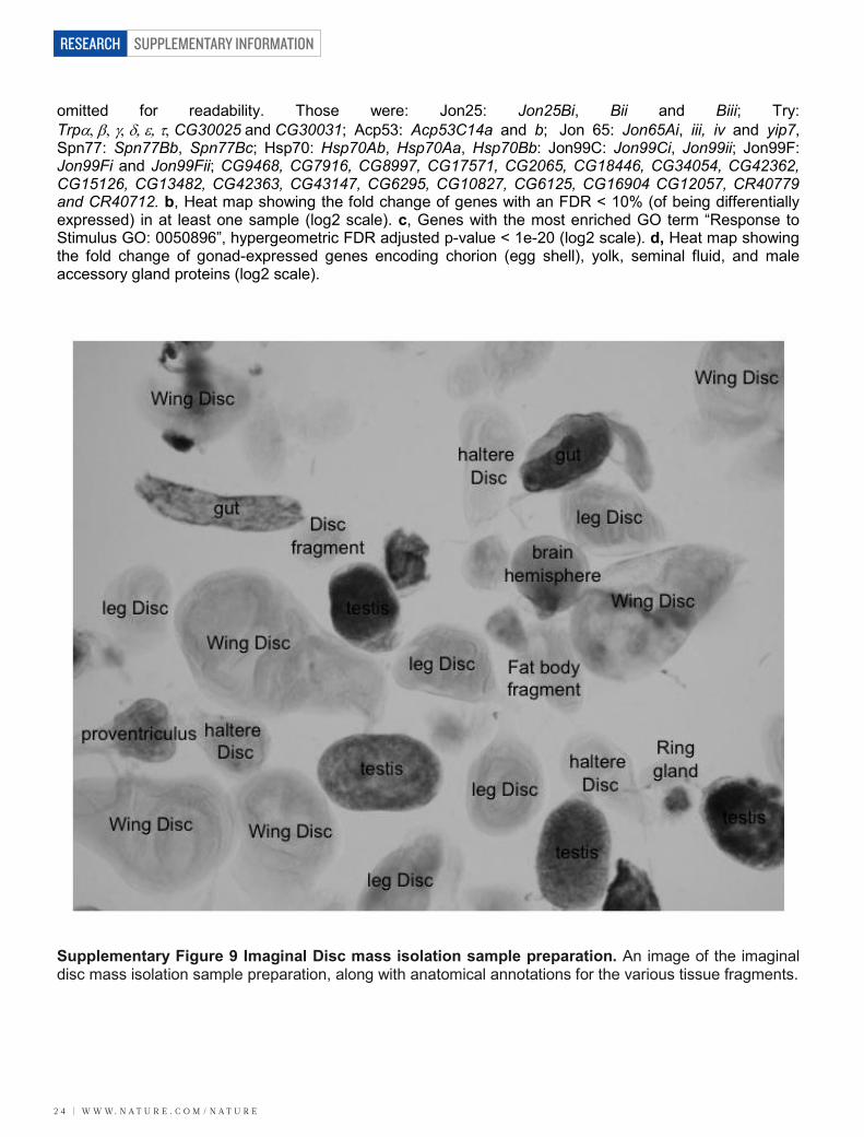
SUPPLEMENTARY INFORMATION
2 4 | W W W. N A T U R E . C O M / N A T U R E
RESEARCH
read libraries down-weighting the average expression.
Supplementary Figure 8 Effects of environmental perturbations on the Drosophila transcriptome, full figure. Adults were treated with the stimulant, caffeine; heavy metals, Cd, Cu and Zn; temperature, cold and heat; and the herbicide, paraquat. a, A genome-wide map of genes that are up or down regulated as a function of Cd treatment. Labeled genes are those that showed a 20-fold (<10% FDR) change in response (linear scale). Genes highlighted in red are those identified previously in larvae50. In Fig. 6, some genes were omitted for readability. Those were: Jon25: Jon25Bi, Bii and Biii; Try: Trpα, β, γ, δ, ε, τ, CG30025 and CG30031; Acp53: Acp53C14a and b; Jon 65: Jon65Ai, iii, iv and yip7, Spn77: Spn77Bb, Spn77Bc; Hsp70: Hsp70Ab, Hsp70Aa, Hsp70Bb: Jon99C: Jon99Ci, Jon99ii; Jon99F: Jon99Fi and Jon99Fii; CG9468, CG7916, CG8997, CG17571, CG2065, CG18446, CG34054, CG42362, CG15126, CG13482, CG42363, CG43147, CG6295, CG10827, CG6125, CG16904 CG12057, CR40779 and CR40712. b, Heat map showing the fold change of genes with an FDR < 10% (of being differentially expressed) in at least one sample (log2 scale). c, Genes with the most enriched GO term “Response to Stimulus GO: 0050896”, hypergeometric FDR adjusted p-value < 1e-20 (log2 scale). d, Heat map showing the fold change of gonad-expressed genes encoding chorion (egg shell), yolk, seminal fluid, and male accessory gland proteins (log2 scale).
Supplementary Figure 9 Imaginal Disc mass isolation sample preparation. An image of the imaginal disc mass isolation sample preparation, along with anatomical annotations for the various
Supplementary Figure 10 Drosophila Body Map. An overview of the tissues collected in the adult and embryo dissections and mass tissue isolations. Maps between the larval progenitor tissues, which were isolated en masse in our sample enriched for Imaginal Discs, and connecting lines indicates corresponding adult tissues.
Supplementary Figure 11 Differential splicing in development and tissues. a, Fraction of splicing events with indicated ∆Ψ values amongst all developmental and tissue samples (black), between just developmental samples (red) and between just tissue samples (green). b, Conservation of cassette exons as a function of ∆Ψ values. c, Frame preservation of cassette exons as a function of ∆Ψ values. read libraries down-weighting the average expression.
Supplementary Figure 8 Effects of environmental perturbations on the Drosophila transcriptome, full figure. Adults were treated with the stimulant, caffeine; heavy metals, Cd, Cu and Zn; temperature, cold and heat; and the herbicide, paraquat. a, A genome-wide map of genes that are up or down regulated as a function of Cd treatment. Labeled genes are those that showed a 20-fold (<10% FDR) change in response (linear scale). Genes highlighted in red are those identified previously in larvae50. In Fig. 6, some genes were omitted for readability. Those were: Jon25: Jon25Bi, Bii and Biii; Try: Trpα, β, γ, δ, ε, τ, CG30025 and CG30031; Acp53: Acp53C14a and b; Jon 65: Jon65Ai, iii, iv and yip7, Spn77: Spn77Bb, Spn77Bc; Hsp70: Hsp70Ab, Hsp70Aa, Hsp70Bb: Jon99C: Jon99Ci, Jon99ii; Jon99F: Jon99Fi and Jon99Fii; CG9468, CG7916, CG8997, CG17571, CG2065, CG18446, CG34054, CG42362, CG15126, CG13482, CG42363, CG43147, CG6295, CG10827, CG6125, CG16904 CG12057, CR40779 and CR40712. b, Heat map showing the fold change of genes with an FDR < 10% (of being differentially expressed) in at least one sample (log2 scale). c, Genes with the most enriched GO term “Response to Stimulus GO: 0050896”, hypergeometric FDR adjusted p-value < 1e-20 (log2 scale). d, Heat map showing the fold change of gonad-expressed genes encoding chorion (egg shell), yolk, seminal fluid, and male accessory gland proteins (log2 scale).
Supplementary Figure 9 Imaginal Disc mass isolation sample preparation. An image of the imaginal disc mass isolation sample preparation, along with anatomical annotations for the various tissue fragments.
Supplementary Figure 10 Drosophila Body Map. An overview of the tissues collected in the adult and embryo dissections and mass tissue isolations. Maps between the larval progenitor tissues, which were isolated en masse in our sample enriched for Imaginal Discs, and connecting lines indicates corresponding adult tissues.
Supplementary Figure 11 Differential splicing in development and tissues. a, Fraction of splicing events with indicated ∆Ψ values amongst all developmental and tissue samples (black), between just developmental samples (red) and between just tissue samples (green). b, Conservation of cassette exons as a function of ∆Ψ values. c, Frame preservation of cassette exons as a function of ∆Ψ values.

W W W. N A T U R E . C O M / N A T U R E | 2 5
SUPPLEMENTARY INFORMATION RESEARCH
read libraries down-weighting the average expression.
Supplementary Figure 8 Effects of environmental perturbations on the Drosophila transcriptome, full figure. Adults were treated with the stimulant, caffeine; heavy metals, Cd, Cu and Zn; temperature, cold and heat; and the herbicide, paraquat. a, A genome-wide map of genes that are up or down regulated as a function of Cd treatment. Labeled genes are those that showed a 20-fold (<10% FDR) change in response (linear scale). Genes highlighted in red are those identified previously in larvae50. In Fig. 6, some genes were omitted for readability. Those were: Jon25: Jon25Bi, Bii and Biii; Try: Trpα, β, γ, δ, ε, τ, CG30025 and CG30031; Acp53: Acp53C14a and b; Jon 65: Jon65Ai, iii, iv and yip7, Spn77: Spn77Bb, Spn77Bc; Hsp70: Hsp70Ab, Hsp70Aa, Hsp70Bb: Jon99C: Jon99Ci, Jon99ii; Jon99F: Jon99Fi and Jon99Fii; CG9468, CG7916, CG8997, CG17571, CG2065, CG18446, CG34054, CG42362, CG15126, CG13482, CG42363, CG43147, CG6295, CG10827, CG6125, CG16904 CG12057, CR40779 and CR40712. b, Heat map showing the fold change of genes with an FDR < 10% (of being differentially expressed) in at least one sample (log2 scale). c, Genes with the most enriched GO term “Response to Stimulus GO: 0050896”, hypergeometric FDR adjusted p-value < 1e-20 (log2 scale). d, Heat map showing the fold change of gonad-expressed genes encoding chorion (egg shell), yolk, seminal fluid, and male accessory gland proteins (log2 scale).
Supplementary Figure 9 Imaginal Disc mass isolation sample preparation. An image of the imaginal disc mass isolation sample preparation, along with anatomical annotations for the various
Supplementary Figure 10 Drosophila Body Map. An overview of the tissues collected in the adult and embryo dissections and mass tissue isolations. Maps between the larval progenitor tissues, which were isolated en masse in our sample enriched for Imaginal Discs, and connecting lines indicates corresponding adult tissues.
Supplementary Figure 11 Differential splicing in development and tissues. a, Fraction of splicing events with indicated ∆Ψ values amongst all developmental and tissue samples (black), between just developmental samples (red) and between just tissue samples (green). b, Conservation of cassette exons as a function of ∆Ψ values. c, Frame preservation of cassette exons as a function of ∆Ψ values.
TissueDevelopmentAll
0.00
0.02
0.04
0.06
0.08
0.10
0.12
Frac
tion
of E
vent
s
90 10080706050403020100
∆Ψ
50-10025-500-25
∆Ψ
Mea
n Ph
astC
ons
Scor
e
50-100 25-50 0-25∆Ψ
Frame 0Frame 1Frame 2
Frac
tion
of E
xons
a b c
0.0
0.2
0.4
0.6
0.8
1.0
0.0
0.2
0.4
0.6
0.8
1.0
read libraries down-weighting the average expression.
Supplementary Figure 8 Effects of environmental perturbations on the Drosophila transcriptome, full figure. Adults were treated with the stimulant, caffeine; heavy metals, Cd, Cu and Zn; temperature, cold and heat; and the herbicide, paraquat. a, A genome-wide map of genes that are up or down regulated as a function of Cd treatment. Labeled genes are those that showed a 20-fold (<10% FDR) change in response (linear scale). Genes highlighted in red are those identified previously in larvae50. In Fig. 6, some genes were omitted for readability. Those were: Jon25: Jon25Bi, Bii and Biii; Try: Trpα, β, γ, δ, ε, τ, CG30025 and CG30031; Acp53: Acp53C14a and b; Jon 65: Jon65Ai, iii, iv and yip7, Spn77: Spn77Bb, Spn77Bc; Hsp70: Hsp70Ab, Hsp70Aa, Hsp70Bb: Jon99C: Jon99Ci, Jon99ii; Jon99F: Jon99Fi and Jon99Fii; CG9468, CG7916, CG8997, CG17571, CG2065, CG18446, CG34054, CG42362, CG15126, CG13482, CG42363, CG43147, CG6295, CG10827, CG6125, CG16904 CG12057, CR40779 and CR40712. b, Heat map showing the fold change of genes with an FDR < 10% (of being differentially expressed) in at least one sample (log2 scale). c, Genes with the most enriched GO term “Response to Stimulus GO: 0050896”, hypergeometric FDR adjusted p-value < 1e-20 (log2 scale). d, Heat map showing the fold change of gonad-expressed genes encoding chorion (egg shell), yolk, seminal fluid, and male accessory gland proteins (log2 scale).
Supplementary Figure 9 Imaginal Disc mass isolation sample preparation. An image of the imaginal disc mass isolation sample preparation, along with anatomical annotations for the various
Supplementary Figure 10 Drosophila Body Map. An overview of the tissues collected in the adult and embryo dissections and mass tissue isolations. Maps between the larval progenitor tissues, which were isolated en masse in our sample enriched for Imaginal Discs, and connecting lines indicates corresponding adult tissues.
Supplementary Figure 11 Differential splicing in development and tissues. a, Fraction of splicing events with indicated ∆Ψ values amongst all developmental and tissue samples (black), between just developmental samples (red) and between just tissue samples (green). b, Conservation of cassette exons as a function of ∆Ψ values. c, Frame preservation of cassette exons as a function of ∆Ψ values.