supplementary materials: efﬁcient moment-based inference ... · supplementary materials:...

Supplementary Materials: Efficient moment-based inference

of admixture parameters and sources of gene flow

Mark Lipson, Po-Ru Loh, Alex Levin, David Reich, Nick Patterson, and Bonnie Berger

41

0 0.1 0.2 0.3 0.4 0.5 0.6 0.7

Surui

Karitiana

Pima

Miao

She

Dai

Lahu

Papuan

Mandenka

Yoruba

MbutiPygmy

Figure S1. Alternative scaffold tree with 11 populations used to evaluate robustness of resultsto scaffold choice. We included Mbuti Pygmy, who are known to be admixed, to helpdemonstrate that MixMapper inferences are robust to deviations from additivity in the scaffold;see Tables S2–S4 for full results. Distances are in drift units.

42

0

0.2

0.4

0.6

0.8

1

Mix

ture

pro

port

ion α

Test population

Figure S2. Summary of mixture proportions α inferred with alternative 9-population scaffoldtrees. We ran MixMapper for all 20 admixed test populations using nine different scaffold treesobtained by removing each population except Papuan one at a time from our full 10-populationscaffold. (Papuan is needed to maintain continental representation.) For each test populationand each scaffold, we recorded the median bootstrap-inferred value of α over all replicateshaving branching patterns similar to the primary topology. Shown here are the means andstandard deviations of the nine medians. In all cases, α refers to the proportion of ancestryfrom the first branch as in Tables 1–3.

43

San

Mbu

tiPyg

my

Bia

kaP

ygm

yB

antu

Ken

yaB

antu

Sou

thA

frica

Man

denk

aY

orub

aM

ozab

iteB

edou

inP

ales

tinia

nD

ruze

Tusc

anS

ardi

nian

Italia

nB

asqu

eFr

ench

Orc

adia

nR

ussi

anA

dyge

iB

aloc

hiB

rahu

iM

akra

niS

indh

iP

atha

nK

alas

hB

urus

hoH

azar

aU

ygur

Cam

bodi

anD

aiLa

huM

iao

She

Tujia

Japa

nese

Han

Han−N

China

Yi

Naxi

Tu Xib

oM

ongo

laH

ezhe

nD

aur

Oro

qen

Yak

utC

olom

bian

Kar

itian

aS

urui

May

aP

ima

Mel

anes

ian

Pap

uan

SanMbutiPygmyBiakaPygmyBantuKenya

BantuSouthAfricaMandenka

YorubaMozabiteBedouin

PalestinianDruze

TuscanSardinian

ItalianBasqueFrench

OrcadianRussianAdygeiBalochiBrahui

MakraniSindhi

PathanKalash

BurushoHazara

UygurCambodian

DaiLahuMiaoShe

TujiaJapanese

HanHan−NChina

YiNaxi

TuXibo

MongolaHezhen

DaurOroqen

YakutColombian

KaritianaSuruiMayaPima

MelanesianPapuan

−1

−0.8

−0.6

−0.4

−0.2

0

0.2

0.4

0.6

Log fold change in f2 values (new array / original HGDP)

Figure S3. Comparison of f2 distances computed using original Illumina vs.San-ascertained SNPs. The heat map shows the log fold change in f2 values obtained fromthe original HGDP data (Li et al., 2008) versus the San-ascertained data (Patterson et al., 2012)used in this study.

44

Drift parameter

0.00 0.02 0.04 0.06 0.08 0.10 0.12 0.14

Surui

Basque

Tujia

Daur

Neandertal

Pima

Hazara

Adygei

Mozabite

Druze

BantuSouthAfrica

Hezhen

Uygur

Oroqen

BantuKenya

Makrani

Sardinian

Palestinian

Brahui

French

Yakut

Balochi

Han.NChinaJapanese

BiakaPygmy

Russian

Lahu

Yi

Pathan

She

Mandenka

MbutiPygmySan

Naxi

Burusho

Denisova

Mongola

Yoruba

Bedouin

Dai

Sindhi

Tuscan

Maya

Orcadian

Colombian

Xibo

Kalash

Han

Karitiana

Italian

Tu

Cambodian

Miao10 s.e.

0

0.5

Migrationweight

Figure S4. TreeMix results on the HGDP. Admixture graph for HGDP populations obtainedwith the TreeMix software, as reported in Pickrell and Pritchard (2012). Figure is reproducedfrom Pickrell and Pritchard (2012) with permission of the authors and under the CreativeCommons Attribution License.

45

0 0.1 0.2 0.3 0.4 0.5 0.6 0.7 0.8 0.9 10

0.5

1

1.5

2

2.5

3

Allele frequency

Pro

babi

lity

dens

ity

IntergenicGenic, non−codingCoding

0 0.02 0.040

5

10

15

Figure S5. Comparison of allele frequency spectra within and outside gene regions. Wedivided the Panel 4 (San-ascertained) SNPs into three groups: those outside gene regions(101,944), those within gene regions but not in exons (58,110), and those within codingregions (3259). Allele frequency spectra restricted to each group are shown for the Yorubapopulation. Reduced heterozygosity within exon regions is evident, which suggests the actionof purifying selection. (Inset) We observe the same effect in the genic, non-coding spectrum; itis less noticeable but can be seen at the edge of the spectrum.

46

A B

A’ B’

B’’A’’C

X’’Y’’

a b

c

r s

C’X’ Y’

P

Figure S6. Schematic of part of an admixture tree. Population C is derived from anadmixture of populations A and B with proportion α coming from A. The f2 distances fromC ′ to the present-day populations A′, B′, X ′, Y ′ give four relations from which we are able toinfer four parameters: the mixture fraction α, the locations of the split points A′′ and B′′ (i.e., rand s), and the combined drift α2a+ (1− α)2b+ c.

47

Table S1. Mixture parameters for simulated data.

AdmixedPop Branch1 + Branch2 # rep α Branch1Loc Branch2Loc MixedDrift

First tree

pop6 pop3 + pop5 500 0.253-0.480 0.078-0.195 / 0.214 0.050-0.086 / 0.143 0.056-0.068

pop6 (true) pop3 + pop5 0.4 0.107 / 0.213 0.077 / 0.145 0.066

Second tree

pop4 pop3 + pop5 500 0.382-0.652 0.039-0.071 / 0.076 0.032-0.073 / 0.077 0.010-0.020

pop4 (true) pop3 + pop5 0.4 0.071 / 0.077 0.038 / 0.077 0.016

pop9 Anc3–7 + pop7 490 0.653-0.915 0.048-0.091 / 0.140 0.013-0.134 / 0.147 0.194-0.216

pop9 (true) Anc3–7 + pop7 0.8 0.077 / 0.145 0.037 / 0.145 0.194

pop10 Anc3–7 + pop7 500 0.502-0.690 0.047-0.091 / 0.140 0.021-0.067 / 0.147 0.151-0.167

pop10 (true) Anc3–7 + pop7 0.6 0.077 / 0.145 0.037 / 0.145 0.150

AdmixedPop2 AdmixedPop1 + Branch3 # rep α2 Branch3Loc

pop8 pop10 + pop2 304 0.782-0.822 0.007-0.040 / 0.040

pop10 + Anc1–2 193 0.578-0.756 0.009-0.104 / 0.148

pop8 (true) pop10 + pop2 0.8 0.020 / 0.039

NOTE.—Mixture parameters inferred by MixMapper for simulated data, followed by true

values for each simulated admixed population. Branch1 and Branch2 are the optimal split

points for the mixing populations, with α the proportion of ancestry from Branch1; topologies

are shown that that occur for at least 20 of 500 bootstrap replicates. The mixed drift parameters

for the three-way admixed pop8 are not well-defined in the simulated tree and are omitted. The

branch “Anc3–7” is the common ancestral branch of pops 3–7, and the branch “Anc1–2” is the

common ancestral branch of pops 1–2. See Figure 2 and the caption of Table 1 for descriptions

of the parameters and Figure 3 for plots of the results.

48

Table S2. Mixture parameters for Europeans inferred with an alternative scaffold tree.

AdmixedPop # rep α Branch1Loc (Anc. N. Eurasian) Branch2Loc (Anc. W. Eurasian) MixedDrift

Adygei 488 0.278-0.475 0.035-0.078 / 0.151 0.158-0.191 / 0.246 0.078-0.093

Basque 273 0.221-0.399 0.055-0.111 / 0.153 0.164-0.194 / 0.244 0.108-0.124

French 380 0.240-0.410 0.054-0.108 / 0.152 0.165-0.192 / 0.245 0.093-0.106

Italian 427 0.245-0.426 0.047-0.103 / 0.152 0.155-0.188 / 0.246 0.095-0.110

Orcadian 226 0.214-0.387 0.061-0.131 / 0.153 0.174-0.197 / 0.244 0.098-0.116

Russian 472 0.296-0.490 0.047-0.093 / 0.151 0.165-0.197 / 0.246 0.080-0.095

Sardinian 390 0.189-0.373 0.045-0.104 / 0.152 0.160-0.190 / 0.245 0.110-0.125

Tuscan 413 0.238-0.451 0.039-0.096 / 0.152 0.153-0.191 / 0.245 0.093-0.111

NOTE.—Mixture parameters inferred by MixMapper for modern-day European populations

using an alternative unadmixed scaffold tree containing 11 populations: Yoruba, Mandenka,

Mbuti Pygmy, Papuan, Dai, Lahu, Miao, She, Karitiana, Suruı, and Pima (see Figure S1). The

parameter estimates are very similar to those obtained with the original scaffold tree (Table 1),

with α slightly higher on average. The bootstrap support for the branching position of “ancient

northern Eurasian” plus “ancient western Eurasian” is also somewhat lower, with the

remaining replicates almost all placing the first ancestral population along the Pima branch

instead. However, this is perhaps not surprising given evidence of European-related admixture

in Pima; overall, our conclusions are unchanged, and the results appear quite robust to

perturbations in the scaffold. See Figure 2A and the caption of Table 1 for descriptions of the

parameters.

49

Table S3. Mixture parameters for other populations modeled as two-way admixturesinferred with an alternative scaffold tree.

AdmixedPop Branch1 + Branch2 # rep α Branch1Loc Branch2Loc MixedDrift

Daur Anc. N. Eurasian + She 264 0.225-0.459 0.005-0.052 / 0.151 0.002-0.014 / 0.016 0.014-0.024

Anc. N. Eurasian + Miao 213 0.235-0.422 0.005-0.049 / 0.151 0.002-0.008 / 0.008 0.014-0.024

Hezhen Anc. N. Eurasian + She 257 0.230-0.442 0.005-0.050 / 0.151 0.002-0.010 / 0.016 0.012-0.034


Oroqen Anc. N. Eurasian + She 336 0.284-0.498 0.010-0.052 / 0.151 0.003-0.015 / 0.016 0.017-0.036


Yakut Anc. N. Eurasian + Miao 246 0.648-0.864 0.004-0.018 / 0.151 0.005-0.008 / 0.008 0.032-0.043

Anc. East Asian + Pima 71 0.917-0.973 0.008-0.020 / 0.045 0.022-0.083 / 0.083 0.028-0.042

Anc. N. Eurasian + She 161 0.664-0.865 0.004-0.018 / 0.151 0.003-0.017 / 0.017 0.030-0.043

Melanesian Dai + Papuan 331 0.168-0.268 0.009-0.011 / 0.011 0.167-0.204 / 0.246 0.089-0.115

Lahu + Papuan 78 0.174-0.266 0.005-0.034 / 0.034 0.167-0.203 / 0.244 0.089-0.118

Han Karitiana + She 167 0.007-0.025 0.026-0.134 / 0.134 0.001-0.006 / 0.016 0.000-0.004

She + Surui 54 0.971-0.994 0.001-0.006 / 0.016 0.017-0.180 / 0.180 0.000-0.003

Anc. N. Eurasian + She 65 0.021-0.080 0.004-0.105 / 0.152 0.001-0.007 / 0.016 0.000-0.003

Pima + She 82 0.009-0.033 0.022-0.085 / 0.085 0.001-0.007 / 0.016 0.000-0.004

NOTE.—Mixture parameters inferred by MixMapper for non-European populations fit as

two-way admixtures using an alternative unadmixed scaffold tree containing 11 populations:

Yoruba, Mandenka, Mbuti Pygmy, Papuan, Dai, Lahu, Miao, She, Karitiana, Suruı, and Pima

(see Figure S1). The results for the first four populations are very similar to those obtained

with the original scaffold tree, except that α is now estimated to be roughly 20% higher.

Melanesian is fit essentially identically as before. Han, however, now appears nearly

unadmixed, which we suspect is due to the lack of an appropriate northern East Asian

population related to one ancestor (having removed Japanese). See Figure 2A and the caption

of Table 1 for descriptions of the parameters; branch choices are shown that that occur for at

least 50 of 500 bootstrap replicates. The “Anc. East Asian” branch is the common ancestral

branch of the four East Asian populations in the unadmixed tree.

50

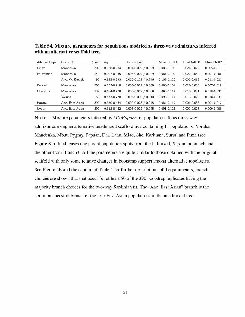
Table S4. Mixture parameters for populations modeled as three-way admixtures inferredwith an alternative scaffold tree.

AdmixedPop2 Branch3 # rep α2 Branch3Loc MixedDrift1A FinalDrift1B MixedDrift2

Druze Mandenka 309 0.958-0.984 0.004-0.009 / 0.009 0.088-0.102 0.021-0.029 0.005-0.013

Palestinian Mandenka 249 0.907-0.935 0.008-0.009 / 0.009 0.087-0.100 0.022-0.030 0.001-0.008

Anc. W. Eurasian 92 0.822-0.893 0.050-0.122 / 0.246 0.102-0.126 0.000-0.019 0.011-0.023

Bedouin Mandenka 303 0.852-0.918 0.006-0.009 / 0.009 0.086-0.101 0.022-0.030 0.007-0.019

Mozabite Mandenka 339 0.684-0.778 0.006-0.009 / 0.009 0.095-0.112 0.010-0.021 0.018-0.032

Yoruba 50 0.673-0.778 0.005-0.010 / 0.010 0.093-0.111 0.010-0.020 0.018-0.031

Hazara Anc. East Asian 390 0.350-0.464 0.009-0.023 / 0.045 0.084-0.119 0.001-0.033 0.004-0.012

Uygur Anc. East Asian 390 0.312-0.432 0.007-0.022 / 0.045 0.091-0.124 0.000-0.027 0.000-0.009

NOTE.—Mixture parameters inferred by MixMapper for populations fit as three-way

admixtures using an alternative unadmixed scaffold tree containing 11 populations: Yoruba,

Mandenka, Mbuti Pygmy, Papuan, Dai, Lahu, Miao, She, Karitiana, Suruı, and Pima (see

Figure S1). In all cases one parent population splits from the (admixed) Sardinian branch and

the other from Branch3. All the parameters are quite similar to those obtained with the original

scaffold with only some relative changes in bootstrap support among alternative topologies.

See Figure 2B and the caption of Table 1 for further descriptions of the parameters; branch

choices are shown that that occur for at least 50 of the 390 bootstrap replicates having the

majority branch choices for the two-way Sardinian fit. The “Anc. East Asian” branch is the

common ancestral branch of the four East Asian populations in the unadmixed tree.

51

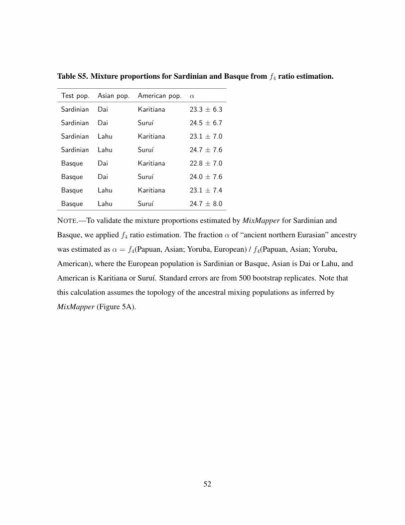
Table S5. Mixture proportions for Sardinian and Basque from f4 ratio estimation.

Test pop. Asian pop. American pop. α

Sardinian Dai Karitiana 23.3 ± 6.3

Sardinian Dai Suruı 24.5 ± 6.7

Sardinian Lahu Karitiana 23.1 ± 7.0

Sardinian Lahu Suruı 24.7 ± 7.6

Basque Dai Karitiana 22.8 ± 7.0

Basque Dai Suruı 24.0 ± 7.6

Basque Lahu Karitiana 23.1 ± 7.4

Basque Lahu Suruı 24.7 ± 8.0

NOTE.—To validate the mixture proportions estimated by MixMapper for Sardinian and

Basque, we applied f4 ratio estimation. The fraction α of “ancient northern Eurasian” ancestry

was estimated as α = f4(Papuan, Asian; Yoruba, European) / f4(Papuan, Asian; Yoruba,

American), where the European population is Sardinian or Basque, Asian is Dai or Lahu, and

American is Karitiana or Suruı. Standard errors are from 500 bootstrap replicates. Note that

this calculation assumes the topology of the ancestral mixing populations as inferred by

MixMapper (Figure 5A).

52

Text S1. f -statistics and population admixture.

Here we include derivations of the allele frequency divergence equations solved by MixMap-

per to determine the optimal placement of admixed populations. These results were first pre-

sented in Reich et al. (2009) and Patterson et al. (2012), and we reproduce them here for com-

pleteness, with slightly different emphasis and notation. We also describe in the final paragraph

(and in more detail in Material and Methods) how the structure of the equations leads to a

particular form of the system for a full admixture tree.

Our basic quantity of interest is the f -statistic f2, as defined in Reich et al. (2009), which is

the squared allele frequency difference between two populations at a biallelic SNP. That is, at

SNP locus i, we define

f i2(A,B) := (pA − pB)2,

where pA is the frequency of one allele in population A and pB is the frequency of the allele in

populationB. This is the same as Nei’s minimum genetic distanceDAB for the case of a biallelic

locus (Nei, 1987). As in Reich et al. (2009), we define the unbiased estimator f i2(A,B), which

is a function of finite population samples:

f i2(A,B) := (pA − pB)2 − pA(1− pA)

nA − 1− pB(1− pB)

nB − 1,

where, for each of A and B, p is the the empirical allele frequency and n is the total number of

sampled alleles.

We can also think of f i2(A,B) itself as the outcome of a random process of genetic history.

In this context, we define

F i2(A,B) := E((pA − pB)2),

the expectation of (pA − pB)2 as a function of population parameters. So, for example, if B is

descended from A via one generation of Wright-Fisher genetic drift in a population of size N ,

then F i2(A,B) = pA(1− pA)/2N .

53

While f i2(A,B) is unbiased, its variance may be large, so in practice, we use the statistic

f2(A,B) :=1

m

m∑i=1

f i2(A,B),

i.e., the average of f i2(A,B) over a set of m SNPs. As we discuss in more detail in Text S2,

F i2(A,B) is not the same for different loci, meaning f2(A,B) will depend on the choice of

SNPs. However, we do know that f2(A,B) is an unbiased estimator of the true average f2(A,B)

of f i2(A,B) over the set of SNPs.

The utility of the f2 statistic is due largely to the relative ease of deriving equations for its

expectation between populations on an admixture tree. The following derivations are borrowed

from (Reich et al., 2009). As above, let the frequency of a SNP i in population X be pX . Then,

for example,

E(f i2(A,B)) = E((pA − pB)2)

= E((pA − pP + pP − pB)2)

= E((pA − pP )2) + E((pP − pB)2) + 2E((pA − pP )(pP − pB))

= E(f i2(A,P )) + E(f i2(B,P )),

since the genetic drifts pA − pP and pP − pB are uncorrelated and have expectation 0. We can

decompose these terms further; if Q is a population along the branch between A and P , then:

E(f i2(A,P )) = E((pA − pP )2)

= E((pA − pQ + pQ − pP )2)

= E((pA − pQ)2) + E((pQ − pP )2) + 2E((pA − pQ)(pQ − pP ))

= E(f i2(A,Q)) + E(f i2(Q,P )).

Here, again, E(pA − pQ) = E(pQ − pP ) = 0, but pA − pQ and pQ − pP are not independent;

54

for example, if pQ − pP = −pP , i.e. pQ = 0, then necessarily pA − pQ = 0. However, pA − pQand pQ − pP are independent conditional on a single value of pQ, meaning the conditional

expectation of (pA − pQ)(pQ − pP ) is 0. By the double expectation theorem,

E((pA − pQ)(pQ − pP )) = E(E((pA − pQ)(pQ − pP )|pQ)) = E(E(0)) = 0.

From E(f i2(A,P )) = E(f i2(A,Q)) +E(f i2(Q,P )), we can take the average over a set of SNPs

to yield, in the notation from above,

F2(A,P ) = F2(A,Q) + F2(Q,P ).

We have thus shown that f2 distances are additive along an unadmixed-drift tree. This

property is fundamental for our theoretical results and is also essential for finding admixtures,

since, as we will see, additivity does not hold for admixed populations.

Given a set of populations with allele frequencies at a set of SNPs, we can use the esti-

mator f2 to compute f2 distances between each pair. These distances should be additive if the

populations are related as a true tree. Thus, it is natural to build a phylogeny using neighbor-

joining (Saitou and Nei, 1987), yielding a fully parameterized tree with all branch lengths in-

ferred. However, in practice, the tree will not exactly be additive, and we may wish to try fitting

some population C ′ as an admixture. To do so, we would have to specify six parameters (in the

notation of Figure S6): the locations on the tree of A′′ and B′′; the branch lengths f2(A′′, A),

f2(B′′, B), and f2(C,C ′); and the mixture fraction. These are the variables r, s, a, b, c, and α.

In order to fit C ′ onto an unadmixed tree (that is, solve for the six mixture parameters), we

use the equations for the expectations F2(C′, Z ′) of the f2 distances between C ′ and each other

population Z ′ in the tree. Referring to Figure S6, with the point admixture model, the allele

55

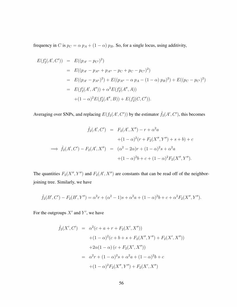
frequency in C is pC = α pA + (1− α) pB. So, for a single locus, using additivity,

E(f i2(A′, C ′)) = E((pA′ − pC′)2)

= E((pA′ − pA′′ + pA′′ − pC + pC − pC′)2)

= E((pA′ − pA′′)2) + E((pA′′ − α pA − (1− α) pB)2) + E((pC − pC′)2)

= E(f i2(A′, A′′)) + α2E(f i2(A

′′, A))

+(1− α)2E(f i2(A′′, B)) + E(f i2(C,C

′)).

Averaging over SNPs, and replacing E(f2(A′, C ′)) by the estimator f2(A′, C ′), this becomes

f2(A′, C ′) = F2(A

′, X ′′)− r + α2a

+(1− α)2(r + F2(X′′, Y ′′) + s+ b) + c

=⇒ f2(A′, C ′)− F2(A

′, X ′′) = (α2 − 2α)r + (1− α)2s+ α2a

+(1− α)2b+ c+ (1− α)2F2(X′′, Y ′′).

The quantities F2(X′′, Y ′′) and F2(A

′, X ′′) are constants that can be read off of the neighbor-

joining tree. Similarly, we have

f2(B′, C ′)− F2(B

′, Y ′′) = α2r + (α2 − 1)s+ α2a+ (1− α)2b+ c+ α2F2(X′′, Y ′′).

For the outgroups X ′ and Y ′, we have

f2(X′, C ′) = α2(c+ a+ r + F2(X

′, X ′′))

+(1− α)2(c+ b+ s+ F2(X′′, Y ′′) + F2(X

′, X ′′))

+2α(1− α) (c+ F2(X′, X ′′))

= α2r + (1− α)2s+ α2a+ (1− α)2b+ c

+(1− α)2F2(X′′, Y ′′) + F2(X

′, X ′′)

56

and

f2(Y′, C ′) = α2r + (1− α)2s+ α2a+ (1− α)2b+ c+ α2F2(X

′′, Y ′′) + F2(Y′, Y ′′).

Assuming additivity within the neighbor-joining tree, any population descended from A′′

will give the same equation (the first type), as will any population descended from B′′ (the

second type), and any outgroup (the third type, up to a constant and a coefficient of α). Thus,

no matter how many populations there are in the unadmixed tree—and assuming there are at

least two outgroups X ′ and Y ′ such that the points X ′′ and Y ′′ are distinct—the system of

equations consisting of E(f2(P,C′)) for all P will contain precisely enough information to

solve for α, r, s, and the linear combination α2a + (1− α)2b + c. We also note the useful fact

that for a fixed value of α, the system is linear in the remaining variables.

57

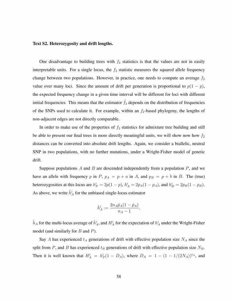
Text S2. Heterozygosity and drift lengths.

One disadvantage to building trees with f2 statistics is that the values are not in easily

interpretable units. For a single locus, the f2 statistic measures the squared allele frequency

change between two populations. However, in practice, one needs to compute an average f2

value over many loci. Since the amount of drift per generation is proportional to p(1 − p),

the expected frequency change in a given time interval will be different for loci with different

initial frequencies. This means that the estimator f2 depends on the distribution of frequencies

of the SNPs used to calculate it. For example, within an f2-based phylogeny, the lengths of

non-adjacent edges are not directly comparable.

In order to make use of the properties of f2 statistics for admixture tree building and still

be able to present our final trees in more directly meaningful units, we will show now how f2

distances can be converted into absolute drift lengths. Again, we consider a biallelic, neutral

SNP in two populations, with no further mutations, under a Wright-Fisher model of genetic

drift.

Suppose populations A and B are descended independently from a population P , and we

have an allele with frequency p in P , pA = p + a in A, and pB = p + b in B. The (true)

heterozygosities at this locus are hiP = 2p(1− p), hiA = 2pA(1− pA), and hiB = 2pB(1− pB).

As above, we write hiA for the unbiased single-locus estimator

hiA :=2nApA(1− pA)

nA − 1,

hA for the multi-locus average of hiA, and H iA for the expectation of hiA under the Wright-Fisher

model (and similarly for B and P ).

Say A has experienced tA generations of drift with effective population size NA since the

split from P , and B has experienced tB generations of drift with effective population size NB.

Then it is well known that H iA = hiP (1 − DA), where DA = 1 − (1 − 1/(2NA))tA , and

58

H iB = hiP (1−DB). We also have

H iA = E(2(p+ a)(1− p− a))

= E(hiP − 2ap+ 2a− 2ap− 2a2)

= hiP − 2E(a2)

= hiP − 2F i2(A,P ),

so 2F i2(A,P ) = hiPDA. Likewise, 2F i

2(B,P ) = hiPDB and 2F i2(A,B) = hiP (DA + DB).

Finally,

H iA +H i

B + 2F i2(A,B) = hiP (1−DA) + hiP (1−DB) + hiP (DA +DB) = 2hiP .

This equation is essentially equivalent to one in Nei (1987), although Nei interprets his version

as a way to calculate the expected present-day heterozygosity rather than estimate the ancestral

heterozygosity. To our knowledge, the equation has not been applied in the past for this second

purpose.

In terms of allele frequencies, the form of hiP turns out to be very simple:

hiP = pA + pB − 2pApB = pA(1− pB) + pB(1− pA),

which is the probability that two alleles, one sampled from A and one from B, are different

by state. We can see, therefore, that this probability remains constant in expectation after any

amount of drift in A and B. This fact is easily proved directly:

E(pA + pB − 2pApB) = 2p− 2p2 = hiP ,

where we use the independence of drift in A and B.

Let hiP := (hiA+ hiB +2f i2(A,B))/2, and let hP denote the true average heterozygosity in P

59

over an entire set of SNPs. Since hiP is an unbiased estimator of (hiA + hiB + 2f i2(A,B))/2, its

expectation under the Wright-Fisher model is hiP . So, the average hP of hiP over a set of SNPs

is an unbiased (and potentially low-variance) estimator of hP . If we have already constructed a

phylogenetic tree using pairwise f2 statistics, we can use the inferred branch length f2(A′, P )

from a present-day population A to an ancestor P in order to estimate hP more directly as

hP = hA+ 2f2(A,P ). This allows us, for example, to estimate heterozygosities at intermediate

points along branches or in the ancestors of present-day admixed populations.

The statistic hP is interesting in its own right, as it gives an unbiased estimate of the het-

erozygosity in the common ancestor of any pair of populations (for a certain subset of the

genome). For our purposes, though, it is most useful because we can form the quotient

dA :=2f2(A,P )

hP,

where the f2 statistic is inferred from a tree. This statistic dA is not exactly unbiased, but by the

law of large numbers, if we use many SNPs, its expectation is very nearly

E(dA) ≈ E(2f2(A,P ))

E(hP )=hPDA

hP= DA,

where we use the fact thatDA is the same for all loci. Thus d is a simple, direct, nearly unbiased

moment estimator for the drift length between a population and one of its ancestors. This allows

us to convert branch lengths from f2 distances into absolute drift lengths, one branch at a time,

by inferring ancestral heterozygosities and then dividing.

For a terminal admixed branch leading to a present-day population C ′ with heterozygosity

hC′ , we divide twice the inferred mixed drift c1 = α2a + (1 − α)2b + c (Figure 2) by the

heterozygosity h∗C′ := hC′ + 2c1. This is only an approximate conversion, since it utilizes a

common value h∗C′ for what are really three disjoint branches, but the error should be very small

with short drifts.

An alternative definition of dA would be 1 − hA/hP , which also has expectation (roughly)

60

DA. In most cases, we prefer to use the definition in the previous paragraph, which allows

us to leverage the greater robustness of the f2 statistics, especially when taken from a multi-

population tree.

We note that this estimate of drift lengths is similar in spirit to the widely-used statistic FST .

For example, under proper conditions, the expectation of FST among populations that have

diverged under unadmixed drift is also 1− (1− 1/(2Ne))t (Nei, 1987). When FST is calculated

for two populations at a biallelic locus using the formula (ΠD − ΠS)/ΠD, where ΠD is the

probability two alleles from different populations are different by state and ΠS is the (average)

probability two alleles from the same population are different by state (as in Reich et al. (2009)

or the measure G′ST in Nei (1987)), then this FST is exactly half of our d. As a general rule,

drift lengths d are approximately twice as large as values of FST reported elsewhere.

61

supplementary materials: efﬁcient moment-based inference ... · supplementary materials:...

Documents