supplementary notes on general physics
TRANSCRIPT

Supplementary Notes on General
Physics
Jyhpyng Wang
c© 2005– by Jyhpyng WangAll rights reserved


Contents
1 Essential Mathematics 1
1.1 Derivatives . . . . . . . . . . . . . . . . . . . . . . . . . . . . . 1
1.2 Integration . . . . . . . . . . . . . . . . . . . . . . . . . . . . . 7
1.3 Taylor Expansion . . . . . . . . . . . . . . . . . . . . . . . . . 16
1.4 Ordinary Differential Equations . . . . . . . . . . . . . . . . . 20
1.5 Fourier Transform . . . . . . . . . . . . . . . . . . . . . . . . . 30
1.6 Volume Elements . . . . . . . . . . . . . . . . . . . . . . . . . 37
1.7 Change of Variables . . . . . . . . . . . . . . . . . . . . . . . . 38
1.8 Diagonalizing a Matrix . . . . . . . . . . . . . . . . . . . . . . 40
1.9 Vector Analysis . . . . . . . . . . . . . . . . . . . . . . . . . . 47
1.10 Calculus in Curved Coordinate Systems . . . . . . . . . . . . . 51
1.11 Vector Formulas . . . . . . . . . . . . . . . . . . . . . . . . . . 56
1.12 Multivariable Taylor Expansion . . . . . . . . . . . . . . . . . 58
1.13 Finding Extrema under Constraints . . . . . . . . . . . . . . . 59
1.14 More to Know about n! . . . . . . . . . . . . . . . . . . . . . 60
1.15 Exercises . . . . . . . . . . . . . . . . . . . . . . . . . . . . . . 63
i

ii Contents
2 Motion of Particles 69
2.1 Space-Time Coordinates and Physical Laws . . . . . . . . . . 69
2.2 Inertial Frames . . . . . . . . . . . . . . . . . . . . . . . . . . 70
2.3 The Cluster Decomposition Postulate . . . . . . . . . . . . . . 73
2.4 Equation of Motion . . . . . . . . . . . . . . . . . . . . . . . . 74
2.5 Inertial Mass and Gravitational Mass . . . . . . . . . . . . . . 75
2.6 Work and Potential Energy . . . . . . . . . . . . . . . . . . . 77
2.7 Separating out Internal Motion . . . . . . . . . . . . . . . . . 79
2.8 The Angular Velocity Pseudovector . . . . . . . . . . . . . . . 80
2.9 Motion in a Rotating Frame . . . . . . . . . . . . . . . . . . . 82
2.10 Foucault Pendulum . . . . . . . . . . . . . . . . . . . . . . . . 83
2.11 Moment of Inertia . . . . . . . . . . . . . . . . . . . . . . . . . 84
2.12 The Shell Theorem of Gravity . . . . . . . . . . . . . . . . . . 89
2.13 The Kepler Problem . . . . . . . . . . . . . . . . . . . . . . . 90
2.14 Exercises . . . . . . . . . . . . . . . . . . . . . . . . . . . . . . 94
3 Oscillators and Waves 105
3.1 Driven Harmonic Oscillators . . . . . . . . . . . . . . . . . . . 105
3.2 Harmonic Generation in Nonlinear Oscillators . . . . . . . . . 108
3.3 Normal Modes of Coupled Oscillators . . . . . . . . . . . . . . 113
3.4 Swinging a Swing . . . . . . . . . . . . . . . . . . . . . . . . . 113
3.5 Waves on a String . . . . . . . . . . . . . . . . . . . . . . . . . 116
3.6 Solutions of the Wave Equation . . . . . . . . . . . . . . . . . 118

Contents iii
3.7 Energy Density of String Waves . . . . . . . . . . . . . . . . . 121
3.8 Wave Propagation through an Interface . . . . . . . . . . . . . 122
3.9 Exercises . . . . . . . . . . . . . . . . . . . . . . . . . . . . . . 124
4 Statistical and Thermal Physics 129
4.1 Thermodynamic Variables and Processes . . . . . . . . . . . . 129
4.2 Entropy in Thermodynamics . . . . . . . . . . . . . . . . . . . 131
4.3 Thermodynamic Potentials . . . . . . . . . . . . . . . . . . . . 140
4.4 Kinetic Theory of Ideal Gas . . . . . . . . . . . . . . . . . . . 144
4.5 Diffusion . . . . . . . . . . . . . . . . . . . . . . . . . . . . . . 147
4.6 Random Walk . . . . . . . . . . . . . . . . . . . . . . . . . . . 150
4.7 Boltzmann Distribution . . . . . . . . . . . . . . . . . . . . . 152
4.8 Sedimentation and Brownian Motion . . . . . . . . . . . . . . 158
4.9 Osmotic Pressure . . . . . . . . . . . . . . . . . . . . . . . . . 159
4.10 Boiling Point . . . . . . . . . . . . . . . . . . . . . . . . . . . 161
4.11 Exercises . . . . . . . . . . . . . . . . . . . . . . . . . . . . . . 164
5 Fluid Mechanics 171
5.1 Convective Derivative . . . . . . . . . . . . . . . . . . . . . . . 171
5.2 Momentum Conservation . . . . . . . . . . . . . . . . . . . . . 173
5.3 Viscosity . . . . . . . . . . . . . . . . . . . . . . . . . . . . . . 176
5.4 Sound Waves . . . . . . . . . . . . . . . . . . . . . . . . . . . 179
5.5 Waves on Water Surface . . . . . . . . . . . . . . . . . . . . . 180
5.6 Kelvin-Helmholtz Instability . . . . . . . . . . . . . . . . . . . 184

iv Contents
5.7 The Reynolds number . . . . . . . . . . . . . . . . . . . . . . 185
5.8 Exercises . . . . . . . . . . . . . . . . . . . . . . . . . . . . . . 187
6 Electrostatics 191
6.1 Gauss’ Law . . . . . . . . . . . . . . . . . . . . . . . . . . . . 191
6.2 Electric Dipole . . . . . . . . . . . . . . . . . . . . . . . . . . 194
6.3 Electric Polarization . . . . . . . . . . . . . . . . . . . . . . . 196
6.4 Capacitors . . . . . . . . . . . . . . . . . . . . . . . . . . . . . 198
6.5 Exercises . . . . . . . . . . . . . . . . . . . . . . . . . . . . . . 200
7 Magnetostatics 203
7.1 Ampere’s Law . . . . . . . . . . . . . . . . . . . . . . . . . . . 203
7.2 Lorentz Force . . . . . . . . . . . . . . . . . . . . . . . . . . . 206
7.3 Force between Current Loops . . . . . . . . . . . . . . . . . . 207
7.4 Vector Potential . . . . . . . . . . . . . . . . . . . . . . . . . . 207
7.5 Magnetic Dipole . . . . . . . . . . . . . . . . . . . . . . . . . . 209
7.6 Magnetization . . . . . . . . . . . . . . . . . . . . . . . . . . . 215
7.7 Exercises . . . . . . . . . . . . . . . . . . . . . . . . . . . . . . 217
8 Electrodynamics 219
8.1 Faraday’s Law . . . . . . . . . . . . . . . . . . . . . . . . . . . 219
8.2 Maxwell Equations . . . . . . . . . . . . . . . . . . . . . . . . 221
8.3 Electromagnetic Waves . . . . . . . . . . . . . . . . . . . . . . 224
8.4 Radiation by Charge Acceleration . . . . . . . . . . . . . . . . 226

Contents v
8.5 Retarded Potentials . . . . . . . . . . . . . . . . . . . . . . . . 227
8.6 Energy Density of Electromagnetic Fields . . . . . . . . . . . . 230
8.7 Inductors and Transformers . . . . . . . . . . . . . . . . . . . 235
8.8 Dipole Radiation . . . . . . . . . . . . . . . . . . . . . . . . . 239
8.9 Radiation from Relativistic Particles . . . . . . . . . . . . . . 240
8.10 Exercises . . . . . . . . . . . . . . . . . . . . . . . . . . . . . . 242
9 Special Relativity 249
9.1 The Mysterious Ether . . . . . . . . . . . . . . . . . . . . . . 249
9.2 Lorentz Transformation . . . . . . . . . . . . . . . . . . . . . . 252
9.3 Simultaneity and Causality . . . . . . . . . . . . . . . . . . . . 256
9.4 Proper Length and Proper Time . . . . . . . . . . . . . . . . . 257
9.5 Addition of Velocity . . . . . . . . . . . . . . . . . . . . . . . 259
9.6 Energy and Momentum . . . . . . . . . . . . . . . . . . . . . . 260
9.7 Four-Vectors . . . . . . . . . . . . . . . . . . . . . . . . . . . . 265
9.8 Transformation of Electromagnetic Fields . . . . . . . . . . . . 270
9.9 Exercises . . . . . . . . . . . . . . . . . . . . . . . . . . . . . . 272
10 Optics 275
10.1 Refraction and Reflection of Plane Waves . . . . . . . . . . . . 275
10.2 Huygen’s principle . . . . . . . . . . . . . . . . . . . . . . . . 282
10.3 Paraxial Approximation and Fresnel’s Diffraction . . . . . . . 284
10.4 Index of Refraction . . . . . . . . . . . . . . . . . . . . . . . . 285
10.5 Clausius-Mossotti Equation . . . . . . . . . . . . . . . . . . . 290

vi Contents
10.6 Light Propagating in Dispersive Media . . . . . . . . . . . . . 291
10.7 Scattering . . . . . . . . . . . . . . . . . . . . . . . . . . . . . 293
10.8 Diffraction of X-Ray . . . . . . . . . . . . . . . . . . . . . . . 295
10.9 Exercises . . . . . . . . . . . . . . . . . . . . . . . . . . . . . . 297
11 Quantum Phenomena 303
11.1 Rayleigh-Jeans Formula for Blackbody Radiation . . . . . . . 303
11.2 Planck’s Theory of Blackbody Radiation . . . . . . . . . . . . 304
11.3 Photoelectric Effect . . . . . . . . . . . . . . . . . . . . . . . . 305
11.4 Taylor’s Interference Experiment . . . . . . . . . . . . . . . . 305
11.5 Emission Spectrum of the Hydrogen Atom . . . . . . . . . . . 306
11.6 Franck-Hertz Experiment . . . . . . . . . . . . . . . . . . . . . 307
11.7 Problem of Specific Heat . . . . . . . . . . . . . . . . . . . . . 307
11.8 Wilson-Sommerfeld Quantization Rule . . . . . . . . . . . . . 308
11.9 Exercises . . . . . . . . . . . . . . . . . . . . . . . . . . . . . . 309
12 Matter Waves 313
12.1 Schrodinger Equation . . . . . . . . . . . . . . . . . . . . . . . 313
12.2 Probabilistic Interpretation of Wavefunction . . . . . . . . . . 314
12.3 Stationary States and State Evolution . . . . . . . . . . . . . 316
12.4 Uncertainty Relation of Position and Momentum . . . . . . . 318
13 Bound States in Quantum Models 323
13.1 Method of Power Expansion . . . . . . . . . . . . . . . . . . . 323

Contents vii
13.2 Harmonic Oscillator . . . . . . . . . . . . . . . . . . . . . . . . 324
13.3 Morse Oscillator . . . . . . . . . . . . . . . . . . . . . . . . . . 326
13.4 Poschl-Teller Oscillator . . . . . . . . . . . . . . . . . . . . . . 328
13.5 Hydrogen Atom . . . . . . . . . . . . . . . . . . . . . . . . . . 331
13.6 Exercises . . . . . . . . . . . . . . . . . . . . . . . . . . . . . . 336
14 Operator Algebra in Quantum Mechanics 339
14.1 Linear Space and Representation . . . . . . . . . . . . . . . . 339
14.2 Uncertainty Principle . . . . . . . . . . . . . . . . . . . . . . . 342
14.3 Eigenvalues of the Angular Momentum . . . . . . . . . . . . . 343
14.4 Operator Algebra of the Harmonic Oscillator . . . . . . . . . . 346
14.5 Quantization of Mechanical Waves . . . . . . . . . . . . . . . 348
14.6 Quantization of Electromagnetic Waves . . . . . . . . . . . . . 349
14.7 Coherent States . . . . . . . . . . . . . . . . . . . . . . . . . . 352
14.8 Quantum Fluctuation of Electromagnetic Waves . . . . . . . . 354
14.9 Exercises . . . . . . . . . . . . . . . . . . . . . . . . . . . . . . 356
A Theory of Measurement Uncertainty 359
A.1 Variance of Arithmetic Means . . . . . . . . . . . . . . . . . . 359
A.2 Sample Variance . . . . . . . . . . . . . . . . . . . . . . . . . 360
A.3 Central Limit Theorem . . . . . . . . . . . . . . . . . . . . . . 361
A.4 Curve Fitting as an Indirect Measurement . . . . . . . . . . . 363
A.5 Linear Regression . . . . . . . . . . . . . . . . . . . . . . . . . 364
A.6 Multivalue fitting with unknown error bars . . . . . . . . . . . 366

viii Contents
A.7 Multivalue fitting with known error bars . . . . . . . . . . . . 367
B Hints of Selected Exercises 369
C Topics to be added 379
D ASCII and Greek Characters 381
D.1 ASCII Characters . . . . . . . . . . . . . . . . . . . . . . . . . 381
D.2 Greek Characters . . . . . . . . . . . . . . . . . . . . . . . . . 382
D.3 Military Phonetic Alphabet . . . . . . . . . . . . . . . . . . . 382

Chapter 1
Essential Mathematics
1.1 Derivatives
The derivative of a continuous function f(x) is usually written as f ′(x) ordf/dx. From its definition
f ′(x) ≡ lim∆x→0
f(x + ∆x)− f(x)
∆x, (1.1)
it is clear that f ′(x) is the slope of the tangent line of the curve y = f(x) at x,and it represents the rate of change of f(x) at x. For instance, if D(t) is thedistance of a particle from the origin at time t, then D′(t) is the instantaneousvelocity of the particle at time t. If V (x) is the potential energy of a particleat position x, then −V ′(x) is the force experienced by the particle at positionx.
The operation of deriving f ′(x) from f(x) is called differentiation. Fromthe definition in Eq. (1.1) it is clear that differentiation is a linear operation.Namely, if h(x) = af(x) + bg(x), where a and b are two constants, thenh′(x) = af ′(x) + bg′(x).
Let us see what is the derivative of a polynomial. Because differentiationis a linear operation, it is sufficient to consider the derivative of xn.
(xn)′ = lim∆x→0
(x + ∆x)n − xn
∆x
1

2 Chapter 1. Essential Mathematics
= lim∆x→0
(Cn1 xn−1 + Cn
2 xn−2∆x + · · ·+ Cnn−1x∆xn−2 + Cn
n∆xn−1)
= nxn−1. (1.2)
If h(x) = f(x)g(x), then
h′(x) = lim∆x→0
f(x + ∆x)g(x + ∆x)− f(x)g(x)
∆x
= lim∆x→0
f(x + ∆x)g(x + ∆x)− f(x)g(x + ∆x)
∆x
+ lim∆x→0
f(x)g(x + ∆x)− f(x)g(x)
∆x= f ′(x)g(x) + g′(x)f(x). (1.3)
This is known as the multiplication rule of differentiation. Let g(x) =1/f(x), then h′(x) = 0. By the multiplication rule we have
f ′(x)g(x) + g′(x)f(x) = 0. (1.4)
Namely
g′(x) = − f ′(x)
f(x)2. (1.5)
From this formula, we obtain (x−n)′ = −nx−n−1.
If h(x) is the composition function of f(x) and g(x), namely h(x) =f [g(x)], then
h′(x) = lim∆x→0
f [g(x + ∆x)]− f [g(x)]
∆x
= lim∆x→0
f [g(x + ∆x)]− f [g(x)]
g(x + ∆x)− g(x)× g(x + ∆x)− g(x)
∆x
= f ′[g(x)]g′(x). (1.6)
This is known as the chain rule of differentiation. As an example, we have[f(x)n]′ = nf(x)n−1f ′(x). If f(x) and f−1(x) are inverse functions of eachother, namely f [f−1(x)] = x, we have
1 = f ′[f−1(x)](f−1)′(x),
namely,
(f−1)′(x) =1
f ′[f−1(x)]. (1.7)

1.1. Derivatives 3
Now we are ready to extend the derivative of xk from an integer k to arational number k. Let k = 1/q where q is an integer, then (x1/q)q = x.Differentiating both sides, by the chain rule we have
1 = q(x1q )q−1(x
1q )′. (1.8)
In other words,
(x1q )′ =
1
qx
1q−1. (1.9)
Now let k = p/q, where p and q are integers. By the chain rule we have
(xpq )′ =
[(xp)
1q
]′=
1
q(xp)
1q−1p xp−1 =
(p
q
)x( p
q )−1. (1.10)
Finally let us consider the derivative of xr when r is a real number. Beforedoing that, we must note that the definition of xr is not as trivial as xp/q
when p and q are integer. The expression xp/q is defined by the numberα that satisfies αq = xp. But what do we mean by xr when r cannot beexpressed as p/q? It turns out that one must use a sequence of rationalnumbers k1 = p1/q1, k2 = p2/q2, k3 = p3/q3, · · · that approaches r to definexr. In other words
xr ≡ limkn→r
xkn . (1.11)
With this definition we have
(xr)′ = lim∆x→0
limkn→r(x + ∆x)kn − limkn→r xkn
∆x
= lim∆x→0
limkn→r
(x + ∆x)kn − xkn
∆x
= limkn→r
knxkn−1 = rxr−1. (1.12)
Note that we have swapped the order of the two limiting process ∆x → 0and kn → r. This is not always safe because in some special cases they maylead to two different values. However, how to do it rigorously is beyond thescope of this lecture.
Now we turn our attention to transcendental functions. Consider thederivative of ax, where a is a real number.
(ax)′ = lim∆x→0
ax+∆x − ax
∆x= ax lim
∆x→0
a∆x − 1
∆x. (1.13)

4 Chapter 1. Essential Mathematics
Assuming the limit in Eq. (1.13) exists, let
b = lim∆x→0
a∆x − 1
∆x. (1.14)
We may rewrite the limit as
b = limn→∞
a1n − 1
1n
, (1.15)
which means for an arbitrarily small ε there exists an M such that for anyn > M we have
b− ε ≤ a1n − 1
1n
≤ b + ε, (1.16)
or equivalently
(1 +
b− ε
n
)n
≤ a ≤(
1 +b + ε
n
)n
. (1.17)
Note that(
1 +b + ε
n
)n
−(
1 +b− ε
n
)n
= 2ε
1
n
n−1∑
k=0
(1 +
b + ε
n
)k (1 +
b− ε
n
)n−1−k . (1.18)
Since we can make ε arbitrarily small by choosing a sufficiently large n, andwhile doing so the term in the square bracket remains finite, it can be seenfrom Eqs. (1.17) and (1.18) that
a = limn→∞
(1 +
b
n
)n
. (1.19)
Let us consider the special case of b = 1. In this case (ax)′ = ax and we have
αn =n∑
k=0
Cnk
(1
n
)k
. (1.20)
Consider another sequence of numbers sn defined by
sn =n∑
k=0
1
k!. (1.21)

1.1. Derivatives 5
Since
Cnk
(1
n
)k
=n(n− 1)(n− 2) . . . (n− k + 1)
k!nk≤ 1
k!, (1.22)
we have αn ≤ sn. Consider yet another sequence of numbers rm(n) (m < n)defined by
rm(n) =m∑
k=0
Cnk
(1
n
)k
= 1 + 1 +(n− 1)
2n+
(n− 1)(n− 2)
6n2. . .
+(n− 1)(n− 2) . . . (n−m + 1)
m!nm−1. (1.23)
Since rm(n) contains only the first m terms of αn and every term in αn ispositive, we have rm(n) ≤ αn ≤ sn. Taking the limit of n →∞ we obtain
sm = limn→∞ rm(n) ≤ lim
n→∞αn ≤ limn→∞ sn. (1.24)
In other words, for any m we have
sm ≤ a ≤ limn→∞ sn. (1.25)
Therefore
a = limn→∞ sn =
∞∑
k=0
1
k!≈ 2.718282 . (1.26)
This is a special number which makes (ax)′ = ax, therefore it is the naturalchoice for the base of the exponential function in calculus. It deserves to berepresented by a special symbol, hence from now on we use e to representthis number.
e = limn→∞
(1 +
1
n
)n
=∞∑
k=0
1
k!≈ 2.718282 . (1.27)
Now we can go back to Eq. (1.13) and write
(ex)′ = ex. (1.28)
Let us define the inverse function of ex to be ln x ≡ logex. Eq. (1.13) can bewritten as
(ax)′ =[(
eln a)x]′
=(ex ln a
)′= (ln a) ex ln a = (ln a) ax. (1.29)

6 Chapter 1. Essential Mathematics
Fig. 1.1: The radius of the arc is 1, and the angle of span is x. The areaenclosed in the small triangle is sin x/2, in the arc is x/2, and in the largetriangle is tan x/2.
From Eqs. (1.7) and (1.28),
ln′(x) =1
eln x=
1
x. (1.30)
To derive the derivative of sin x and cos x, we note that for small x,sin x ≤ x ≤ tan x as shown in Fig. 1.1. Therefore
1 ≤ limx→0
x
sin x≤ lim
x→0
1
cos x= 1, (1.31)
hence
limx→0
sin x
x= 1. (1.32)
We will also need the following limit.
limx→0
1− cos x
x= 0. (1.33)
To prove Eq. (1.33), let us note
1− cos x
x=
1− cos2 x
x(1 + cos x)=
sin2 x
x(1 + cos x). (1.34)
Since
limx→0
sin x
x= 1, (1.35)
limx→0
sin x
1 + cos x= 0, (1.36)
1.2. Integration 7
we have Eq. (1.33). With Eqs. (1.32) and (1.33), we can derive
sin′ x = lim∆x→0
sin x cos(∆x) + cos x sin(∆x)− sin x
∆x= cos x. (1.37)
cos′ x = lim∆x→0
cos x cos(∆x)− sin x sin(∆x)− cos x
∆x= − sin x. (1.38)
1.2 Integration
Consider a continuous function f(x) defined in [a, b]. Let us divide [a, b]into n intervals [xi, xi+1], where i = 1, 2, · · · , n, x1 = a, xn+1 = b, andxi+1 − xi = ∆x = (b − a)/n. In each interval we select an arbitrary samplepoint xi ∈ (xi, xi+1). Integration of a function f(x) from a to b is defined by
∫ b
af(x) dx ≡ lim
∆x→0
n∑
i=1
f(xi)∆x. (1.39)
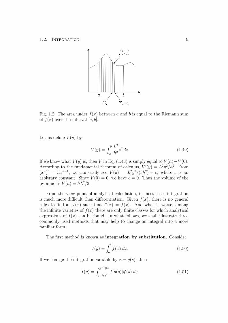
It is known as the Riemann sum of f(x) over the interval [a, b], whichrepresents the area under the curve y = f(x) between x = a and x = b asshown in Fig. 1.2. To have a well-defined Riemann sum, it is important thatthe limit in Eq. (1.39) does not depend on the choice of xi. To prove that,let us first consider the following function defined in [a, b].
g(x) = f(x)− f(b)− f(a)
b− a(x− a)− f(a). (1.40)
Since g(a) = g(b) = 0, there is some real number c ∈ [a, b] such that g(c) ismaximum or minimum, hence g′(c) = 0. Then we have
f ′(c) =f(b)− f(a)
b− a. (1.41)
For a different choice x′i in Eq. (1.39), we have
lim∆x→0
n∑
i=1
[f(xi)− f(x′i)] ∆x ≤ lim∆x→0
n∑
i=1
|f(xi)− f(x′i)|∆x
= lim∆x→0
n∑
i=1
|f ′(ci)| (∆x)2
≤ lim∆x→0
n∑
i=1
M(∆x)2
= lim∆x→0
M(b− a)∆x = 0, (1.42)

8 Chapter 1. Essential Mathematics
where ci is some number in between xi and x′i, and M is the maximum valueof |f ′(x)| in [a, b]. Now consider the integration
I(y) =∫ y
y0
f(x) dx, (1.43)
where y0 < y is an arbitrary starting point. The derivative of I(y) is
I ′(y) = lim∆y→0
∫ y+∆yy0
f(x) dx− ∫ yy0
f(x) dx
∆y
= lim∆y→0
∫ y+∆yy f(x) dx
∆y= f(y). (1.44)
This is known as the fundamental theorem of calculus. Hence if I ′(x) =f(x), we have
∫ b
af(x) dx =
∫ b
y0
f(x) dx−∫ a
y0
f(x) dx = I(b)− I(a). (1.45)
Note that the condition I ′(x) = f(x) does not determine I(x) completely.An arbitrary constant can be added to I(x) without changing I ′(x). Wemust know the value of I(x) for at least one x to determine the constant c.In Eq. (1.43) the definition itself requires that I(y0) = 0. Therefore if weredefine I(x) by the equation I ′(x) = f(x) instead of Eq. (1.43), we maywrite
I(y) =∫ y
f(x) dx + c, (1.46)
where∫ y f(x) dx represents any function whose derivative is f(x) and c is to
be determined by the value of I(x) at some x.
Example 1.1. To demonstrate the usefulness of the fundamental theoremof calculus, let us calculate the volume V of a pyramid shown in Fig. 1.3. Wecan cut the pyramid into n slices in the direction parallel to the base planeof the pyramid. At a distance zi from the tip of the pyramid, the area of theith slice is L2z2
i /h2, where L is the side-length of the base and h is the height
of the pyramid. The sum of the volume of all the slices can be written as
V =n∑
i
L2z2i
h2∆z. (1.47)
In the limit of ∆z → 0,
V =∫ h
0
L2
h2z2 dz. (1.48)
1.2. Integration 9
Fig. 1.2: The area under f(x) between a and b is equal to the Riemann sumof f(x) over the interval [a, b].
Let us define V (y) by
V (y) =∫ y
y0
L2
h2z2 dz. (1.49)
If we know what V (y) is, then V in Eq. (1.48) is simply equal to V (h)−V (0).According to the fundamental theorem of calculus, V ′(y) = L2y2/h2. From(xn)′ = nxn−1, we can easily see V (y) = L2y3/(3h2) + c, where c is anarbitrary constant. Since V (0) = 0, we have c = 0. Thus the volume of thepyramid is V (h) = hL2/3.
From the view point of analytical calculation, in most cases integrationis much more difficult than differentiation. Given f(x), there is no generalrules to find an I(x) such that I ′(x) = f(x). And what is worse, amongthe infinite varieties of f(x) there are only finite classes for which analyticalexpressions of I(x) can be found. In what follows, we shall illustrate threecommonly used methods that may help to change an integral into a morefamiliar form.
The first method is known as integration by substitution. Consider
I(y) =∫ b
af(x) dx. (1.50)
If we change the integration variable by x = g(s), then
I(y) =∫ g−1(b)
g−1(a)f [g(s)]g′(s) ds. (1.51)

10 Chapter 1. Essential Mathematics
Fig. 1.3: A pyramid and a thin slice parallel to the base plane. The volumeof the pyramid is equal to the sum of the volume of all the infinitesimallythin slices.
For some substitutions, f [g(s)]g′(s) is easier to integrate than f(x).
Example 1.2. It is not obvious how to integrate
I(y) =∫ y
0
1
x2 + 1dx. (1.52)
By substituting x = tan θ and dx = sec2 θ dθ, the integration can be reducedto
I(y) =∫ tan−1 y
0dθ = tan−1 y. (1.53)
Example 1.3.
I =∫ 1
0
√1− x2 dx. (1.54)
By substituting x = sin θ and dx = cos θ dθ, the integration can be reducedto
I =∫ π/2
0cos2 θ dθ =
∫ π/2
0
1 + cos(2θ)
2dθ =
π
4. (1.55)
Because the equation for a circle of unit radius in the first quadrant is y(x) =√1− x2, Eq. (1.54) represents the area of a circle in the first quadrant, as
shown in Fig. 1.4. Hence the area of a full circle of unit radius is π.

1.2. Integration 11
Fig. 1.4: The part of a circle in the first quadrant. Its area is equal to thesum of the area of all the infinitesimally thin strips.
Example 1.4. Consider the arc length of a parabolic described by y = x2/2.The line element is
ds =√
dx2 + dy2 =
√√√√1 +
(dy
dx
)2
dx =√
1 + x2 dx (1.56)
Hence the arc length from x = 0 to x = a is
s(a) =∫ a
0
√1 + x2 dx. (1.57)
Define
sinh x ≡ ex − e−x
2,
cosh x ≡ ex + e−x
2. (1.58)
We have
1 + sinh2 x = cosh2 xd
dxsinh x = cosh x,
d
dxcosh x = sinh x. (1.59)
Let x = sinh u. The integration becomes
s(a) =∫ sinh−1 a
0cosh2 u du =
∫ sinh−1 a
0
cosh 2u + 1
2du

12 Chapter 1. Essential Mathematics
=
(sinh 2u
4+
1
2u
)∣∣∣∣∣sinh−1 a
0
=1
2
[a√
a2 + 1 + ln(a +
√a2 + 1
)]. (1.60)
Example 1.5.
I(y) =∫ y
0
1
cos xdx. (1.61)
By substituting u = tan(x/2), we have
cos x =1− u2
1 + u2,
sin x =2u
1 + u2,
dx =2
1 + u2du. (1.62)
This is a well-known substitution to reduce rational expressions of trigonom-etry functions to rational functions. Hence we have
I(y) =∫ y
0
1
cos xdx =
∫ tan(y/2)
0
2
1− u2du
=∫ tan(y/2)
0
(1
1 + u+
1
1− u
)du
= ln(
1 + u
1− u
)∣∣∣∣tan(y/2)
0
= ln
(1 + u2
1− u2+
2u
1− u2
)∣∣∣∣∣tan(y/2)
0
= ln (sec y + tan y). (1.63)
The second method is known as integration by parts. It is based onthe identity [u(x)v(x)]′ = u(x)v′(x) + v(x)u′(x) which implies
∫ b
au(x)v′(x) dx =
∫ b
a[u(x)v(x)]′dx−
∫ b
av(x)u′(x) dx
= u(b)v(b)− u(a)v(a)−∫ b
av(x)u′(x) dx. (1.64)
The technique is useful when v(x)u′(x) is easier to integrate than u(x)v′(x).

1.2. Integration 13
Example 1.6. Consider
I =∫ π/2
0x cos x dx. (1.65)
Let v(x) = sin x and u(x) = x, then the integral can be reduced to
I =π
2sin
π
2−
∫ π/2
0sin x dx. (1.66)
Example 1.7.
I(y) =∫ y
1ln x dx. (1.67)
Let v(x) = x and u(x) = ln x, then the integral can be reduced to
I(y) = y ln y −∫ y
1dx = y ln y − y + 1. (1.68)
Example 1.8.
I(y) =∫ y
0tan−1 x dx. (1.69)
Let v(x) = x and u(x) = tan−1 x, then integration by parts leads to
I(y) = y tan−1 y −∫ y
0
x
1 + x2dx. (1.70)
Substituting s = x2 + 1 and ds = 2xdx,
I(y) = y tan−1 y −∫ y2+1
1
1
2sds = y tan−1 y − 1
2ln(y2 + 1). (1.71)
The third method, known as integration by partial fractions, can beused for the integration of rational functions. Consider the integration of arational function
∫f(x) dx =
∫ p(x)
q(x)dx, (1.72)
where p(x) and q(x) are polynomials of x. If the order of p(x) is larger thanor equal to that of q(x), we may reduce the integration to
∫f(x) dx =
∫h(x) dx +
∫ r(x)
q(x)dx, (1.73)

14 Chapter 1. Essential Mathematics
where h(x) is a polynomial and the order of r(x) is smaller than that of q(x).Since we already know how to integrate h(x), we shall consider only the casein which the order of p(x) is smaller than that of q(x). Let us assume theorder of q(x) is n and the n roots of q(x) are ri (i = 1, 2, . . . n), then we mayexpress f(x) as
p(x)
q(x)=
n∑
i=1
ai
x− ri
, (1.74)
where ai (i = 1, 2, . . . n) are n constants. The reason we can always do thatis because the order of p(x) is at most n− 1, hence we have
p(x) =n−1∑
i=0
cixi, (1.75)
where ci (i = 0, 2, . . . n − 1) are n constants. For any set of ci we maysolve Eq. (1.74) to find the corresponding set of ai. A unique solution existsbecause the number of ci is the same as that of ai. Once we have done thedecomposition in Eq. (1.74), the integration of f(x) becomes trivial.
Finally, we note that some useful integrals in physics are difficult to eval-uate directly, but can be evaluated by introducing another dimension, asshown in the following examples.
Example 1.9. To evaluate
I(α) =∫ ∞
−∞e−αx2
dx, (1.76)
one may evaluate the following integral first.
I2(1) =∫ ∞
−∞e−x2
dx∫ ∞
−∞e−y2
dy =∫ ∞
−∞
∫ ∞
−∞e−(x2+y2)dxdy. (1.77)
By changing variables to the polar coordinates, we have
I2(1) =∫ ∞
0
∫ 2π
0e−r2
rdrdθ = −π e−r2∣∣∣∞0
= π. (1.78)
Therefore
I(1) =∫ ∞
−∞e−x2
dx =√
π. (1.79)
Changing variable from x to√
αx, we obtain
I(α) =∫ ∞
−∞e−αx2
dx =
√π
α. (1.80)

1.2. Integration 15
Example 1.10. To evaluate
I2n(α) =∫ ∞
−∞x2ne−αx2
dx, (1.81)
one may differentiate Eq. (1.80) with respect to α n times.
I2(α) = − d
dα
∫ ∞
−∞e−αx2
dx =1
2α−
32√
π, (1.82)
I4(α) =
(− d
dα
)2 ∫ ∞
−∞e−αx2
dx =1
2
3
2α−
52√
π, (1.83)
...
I2n(α) =
(− d
dα
)n ∫ ∞
−∞e−αx2
dx =(2n)!
n!22nα−
2n+12√
π. (1.84)
Example 1.11.
I =∫ ∞
0
sin x
xdx. (1.85)
To get rid of the x in the denominator which makes the integration difficult,we may evaluate the following function first.
g(y; ε) =∫ ∞
ε
e−xy sin x
xdx, (1.86)
where ε is a positive constant much smaller than 1. Differentiate with respectto y, we have
g′(y; ε) = −∫ ∞
εe−xy sin x dx = −
∫ ∞
ε
e−xy+ix − e−xy−ix
2idx
=i
2
[−eε(i−y)
i− y+−e−ε(i+y)
i + y
]. (1.87)
Expanding eε(i−y) and e−ε(i+y) to the second order of ε, we have
g′(y; ε) ≈ − 1
1 + y2+
ε2
2. (1.88)

16 Chapter 1. Essential Mathematics
From Eq. (1.53) we have
g(y; ε) ≈ − tan−1 y +ε2
2y + c. (1.89)
Because Eq. (1.89) is valid for any ε as long as it is sufficiently small, for asufficiently large y we have
g(y; 1/y) ≈ − tan−1 y +1
2y+ c. (1.90)
Let y → ∞, the left-hand side of Eq. (1.90) approaches zero, therefore c =π/2. Now let y be a small number and remember again that Eq. (1.89) isvalid for any ε as long as it is sufficiently small, we have
g(y; y) ≈ − tan−1 y +y3
2+
π
2. (1.91)
Let y → 0, we have
∫ ∞
0
sin x
xdx =
π
2. (1.92)
1.3 Taylor Expansion
Consider a continuous function f(x) in the neighborhood of a fixed point a.If f(x) is a polynomial, we have
f(x) = f(a) +n∑
k=1
ck(x− a)k, (1.93)
where ck is the coefficients. Differentiating both sides by m times and sub-stituting in x = a, we have
f (m)(a) = cmm!, (1.94)
therefore cm = f (m)(a)/m! . If f(x) is a not a polynomial, intuitively wecan use a polynomial to approximate it. The more complex f(x) is, thehigher-order polynomial is needed. Hence we can write
f(x) ≈ f(a) +n∑
k=1
f (k)(a)
k!(x− a)k. (1.95)
1.3. Taylor Expansion 17
This is known as the Taylor expansion of f(x) around a.
In Taylor expansion, in principle n can approach infinity. But in practiceat which n should we truncate the series? To answer this question we needto know how good the approximation is. Let us rewrite the Taylor expansionas
f(x) = f(a) +n∑
k=1
f (k)(a)
k!(x− a)k + Rn(x, a), (1.96)
where Rn(x, a) is the nth remainder. Now we shall estimate how large|Rn(x, a)| can be. In the following Taylor expansion, consider b to be fixedand the point of expansion a to be variable.
f(b) = f(a) +n∑
k=1
f (k)(a)
k!(b− a)k + Rn(b, a). (1.97)
Differentiating Eq. (1.97) with respect to a, from the multiplication rule itbecomes
0 = f ′(a) +n∑
k=1
[f (k+1)(a)
k!(b− a)k − f (k)(a)
(k − 1)!(b− a)k−1
]+ R′
n(b, a). (1.98)
The second term in the bracket for k = i cancels the first term in the bracketfor k = i + 1, therefore almost all terms cancel out and we are left with
0 =f (n+1)(a)
n!(b− a)n + R′
n(b, a). (1.99)
Integrating with respect to a, we obtain
Rn(b, a) =∫ a
y0
−f (n+1)(x)
n!(b− x)n dx + c. (1.100)
Because Rn(b, b) = 0, we have
c =∫ b
y0
f (n+1)(x)
n!(b− x)n dx, (1.101)
hence
Rn(b, a) =∫ b
a
f (n+1)(x)
n!(b− x)n dx. (1.102)
We can find the upper bound of |Rn(b, a)| by
|Rn(b, a)| ≤∫ b
a
|f (n+1)(x)|n!
|(b− x)n| dx ≤ M|(b− a)n+1|
(n + 1)!, (1.103)

18 Chapter 1. Essential Mathematics
where M is assumed to be the common upper bound of |f (n+1)(x)| in [a, b] forall n. Because (n+1)! À |(b−a)n+1| for sufficiently large n, limn→∞ |Rn(b, a)| =0 if M exists.
As an example, let us find the Taylor expansion of ex around zero. Be-cause dex/dx = ex,
ex =∞∑
k=0
xk
k!. (1.104)
Let x = 1, we have
e =∞∑
k=0
1
k!≈ 2.718282 . (1.105)
Similarly, the Taylor expansions for cos x and sin x around zero are
cos x =∞∑
k=0
(−1)k
(2k)!x2k,
sin x =∞∑
k=0
(−1)k
(2k + 1)!x2k+1. (1.106)
Comparing Eq. (1.104) with Eq. (1.106), we have the Euler formula
eix = cos x + i sin x. (1.107)
An important application of Taylor expansion is numerical calculation.For example, a simple method for calculating the numerical value of π isusing Taylor expansion in Eq. (1.52).
π
4=
∫ 1
0
1
x2 + 1dx
=∫ 1
0(1− x2 + x4 − x6 + · · ·) dx
= 1− 1
3+
1
5− 1
7+ · · ·
=∞∑
n=0
(1
4n + 1− 1
4n + 3
). (1.108)
For large n, this sequence is essentially 1/(8n2), hence it converges ratherslowly. Noting that tan(π/8) =
√2− 1, it is better to use
π
8=
∫ √2−1
0
1
x2 + 1dx

1.3. Taylor Expansion 19
=∫ √
2−1
0(1− x2 + x4 − x6 + · · ·) dx
= (√
2− 1)− (√
2− 1)3
3+
(√
2− 1)5
5− (
√2− 1)7
7+ · · · . (1.109)
This series converges much faster because√
2−1 is significantly smaller than1.
In order to extend the exponential function to the complex domain, wemay use Eq. (1.104) as the definition of ez when z is a complex number. Forany two complex numbers y and z,
eyez =
( ∞∑
k=0
yk
k!
) ( ∞∑
m=0
zm
m!
)
=∞∑
k=0
∞∑
m=0
ykzm
k!m!
=∞∑
k=0
∞∑
n=k
ykzn−k
k!(n− k)!
n!
n!
=∞∑
n=0
n∑
k=0
ykzn−k
k!(n− k)!
n!
n!
=∞∑
n=0
(y + z)n
n!
= e(y+z). (1.110)
This allows us to define, for z = x + iy, ez = exeiy = ex(cos y + i sin y), andconsequently ln z = ln(|z|eiθ) = ln |z| + i arg z. Moreover, uz can be definedas ez ln u. For any three complex numbers u, y and z,
(uz)y = ey ln(uz) = ey ln(ez ln u). (1.111)
If −π < Im(z ln u) ≤ π, we may write
ln(ez ln u) = z ln u, (1.112)
otherwise
ln(ez ln u) = z ln u− 2nπi, (1.113)
where n is an integer that ensures −π < Im(z ln u−2nπi) ≤ π. Eqs. (1.111)–(1.113) show that under the restriction −π < Im(z ln u) ≤ π we have
(uz)y = ey ln(uz) = ey ln(ez ln u) = eyz ln u = uyz. (1.114)
Under proper restrictions, Eqs. (1.110) and (1.114) extend the characteristicsof the real exponential function to the complex domain.

20 Chapter 1. Essential Mathematics
1.4 Ordinary Differential Equations
An equation that contains differential operators in it is called a differentialequation. The order of the differential equation is marked by the highestorder of the differential operator in the equation. In physics it often occursthat the rate of change of some variable is a function of the variable itself.In such cases the equation describing that variable is a differential equation.For example, the deceleration of a free-falling particle in air is a function ofits speed, and we need to find out from the differential equation dv/dt = f(v)how v change with t. A common form of first-order differential equation is thefollowing, and it can be solved by the method of separation of variables.
dx
dt= f(x)g(t) =⇒
∫ dx
f(x)=
∫g(t)dt. (1.115)
Example 1.12. Consider
dx
dt=
x(1− x)
t. (1.116)
Separation of variables leads to
∫ dx
x(1− x)=
∫ dt
t. (1.117)
The solution is
ln(
x
1− x
)= ln t + c1, (1.118)
where c1 is a constant. Solving x in terms of t, we obtain
x =t
t + c2
. (1.119)
The constant c2 = e−c1 can be determined by the initial value of the equation.For example, if we know at t = 1, x = 1/2, then c2 = 1 in the above equation.
Another form of first-order differential equation often encountered inphysics is the linear equation.
dx
dt+ f(t)x = g(t). (1.120)
1.4. Ordinary Differential Equations 21
Let us solve first for the special case g(t) = 0. Separation of variable yields
ln x = −∫ t
t0f(s) ds + c0, (1.121)
or
x(t) = c exp[−
∫ t
t0f(s) ds
], (1.122)
where c = x(t0). We can now modify this solution to suit for the case g(t) 6= 0.The method is known as variation of parameters. In Eq. (1.122), c is aparameter that does not depend on t. If we force it to change with t, thenthis dependence will generate new terms in Eq. (1.120) to cancel g(t). Let
x(t) = c(t)h(t), (1.123)
where c is now a function of t and
h(t) = exp[−
∫ t
t0f(s) ds
]. (1.124)
Substitute x(t) = c(t)h(t) into Eq. (1.120), we have
dc(t)
dth(t) = g(t), (1.125)
hence
dc(t)
dt=
g(t)
h(t), (1.126)
or
c(t) =∫ t
t0
g(u)
h(u)du + x(t0). (1.127)
Eqs. (1.123) and (1.126) can be written as
d
dt
[x(t)
h(t)
]=
g(t)
h(t). (1.128)
The function 1/h(t) is called the integration factor. Because
d
dt
[1
h(t)
]= − 1
h2(t)
dh(t)
dt=
f(t)
h(t), (1.129)
22 Chapter 1. Essential Mathematics
by multiplying both sides of Eq. (1.120) with the integration factor 1/h(t),it is reduced to Eq. (1.128). The solution is
x(t) = h(t)∫ t
t0
g(u)
h(u)du + x(t0)h(t). (1.130)
Example 1.13. Consider the equation
dx
dt+ tx = t3. (1.131)
The integration factor 1/h(t) is obviously et2/2. Multiplying both sides by1/h(t), the equation becomes
d
dt
(et2/2x
)= et2/2t3. (1.132)
The solution is
et2/2x =∫ t
t0es2/2s3 ds + c0. (1.133)
Using integration by parts by setting u = s2 and dv = ses2/2 ds, one obtains
∫ t
t0es2/2s3 ds = t2et2/2 − 2et2/2 + c. (1.134)
Therefore
et2/2x(t) = t2et2/2 − 2et2/2 + c, (1.135)
or equivalently
x = t2 − 2 + ce−t2/2. (1.136)
There is no general method to solve high-order differential equations ex-cept when the equation is linear and has constant coefficients,
dnx
dtn+ a1
dn−1x
dtn−1+ a2
dn−2x
dtn−2+ · · ·+ anx = f(t), (1.137)
where a1, a2, · · · , an are arbitrary constants. If x1 and x2 are two solutions ofEq. (1.137), then their difference x1− x2 satisfies the homogeneous equation
dnx
dtn+ a1
dn−1x
dtn−1+ a2
dn−2x
dtn−2+ · · ·+ anx = 0. (1.138)

1.4. Ordinary Differential Equations 23
Therefore we only need to find one particular solution xp of Eq. (1.137) inaddition to the solutions xh of the homogeneous Eq. (1.138). All the solutionsof Eq. (1.137) can be written as x = xp + xh. The solution xh has the form
xh = ceλt, (1.139)
where λ satisfies
λn + a1λn−1 + a2λ
n−2 + · · ·+ an = 0. (1.140)
Eq. (1.140) has n roots, therefore the general solution for xh is
xh =n∑
i=1
cieλit, (1.141)
where the coefficients ci are determined by specifying the initial conditions
x(0),dx
dt
∣∣∣∣∣x=0
, . . .d(n−1)x
dt(n−1)
∣∣∣∣∣x=0
.
If there are m roots of the same λ in Eq. (1.140), the m linearly independentsolutions corresponding to this λ are tmeλt (m = 0, 1, . . . , m − 1). This canbe seen from the following equation:
(d
dt− λ
)ctkeλt = cktk−1eλt. (1.142)
There is no general method to find xp. For simple cases xp can be derivedby guessing from f(t). In what follows we give six examples of such guesswork.
Example 1.14.
d2x
dt2+ 3
dx
dt+ 2x = t2. (1.143)
First we solve the homogeneous equation
d2x
dt2+ 3
dx
dt+ 2x = 0. (1.144)
Substituting Eq. (1.138) into Eq. (1.144), we have
λ2 + 3λ + 2 = 0. (1.145)

24 Chapter 1. Essential Mathematics
The solutions are λ = −1 and λ = −2, therefore
xh = c1e−t + c2e
−2t. (1.146)
For the particular solution, we guess
xp = at2 + bt + c. (1.147)
Substituting this into Eq. (1.143), we have
2at2 + (6a + 2b)t + (2a + 3b + 2c) = t2. (1.148)
Comparing the coefficients of both sides, we have
2a = 1, 6a + 2b = 0, 2a + 3b + 2c = 0. (1.149)
That is
a =1
2, b = −3
2, c =
7
4. (1.150)
Therefore the particular solution is
xp =1
2t2 − 3
2t +
7
4, (1.151)
and the general solution is
x = xp + xh =1
2t2 − 3
2t +
7
4+ c1e
−t + c2e−2t. (1.152)
Example 1.15.
d2x
dt2− 4
dx
dt− 5x = 3et. (1.153)
First we solve the homogeneous equation
d2x
dt2− 4
dx
dt− 5x = 0. (1.154)
Since the roots of
λ2 − 4λ− 5 = 0 (1.155)
are λ = −1 and λ = 5, we have
xh = c1e−t + c2e
5t. (1.156)

1.4. Ordinary Differential Equations 25
For the particular solution, we guess
xp = aet. (1.157)
Substituting this into Eq. (1.153), we have
(a− 4a− 5a)et = 3et. (1.158)
Comparing the coefficients of both sides, we have
a = −3
8. (1.159)
Therefore the particular solution is
xp = −3
8et, (1.160)
and the general solution is
x = xp + xh = −3
8et + c1e
−t + c2e5t. (1.161)
Example 1.16.
d2x
dt2− 4
dx
dt+ 3x = sin t. (1.162)
First we solve the homogeneous equation
d2x
dt2− 4
dx
dt+ 3x = 0. (1.163)
Since the roots of
λ2 − 4λ + 3 = 0 (1.164)
are λ = 1 and λ = 3, we have
xh = c1et + c2e
3t. (1.165)
For the particular solution, we guess
xp = a sin t + b cos t. (1.166)
Substituting this into Eq. (1.162), we have
(2a + 4b) sin t + (−4a + 2b) cos t = sin t. (1.167)

26 Chapter 1. Essential Mathematics
Comparing the coefficients of both sides, we have
2a + 4b = 1, −4a + 2b = 0. (1.168)
That is
a =1
10, b =
1
5. (1.169)
Therefore the particular solution is
xp =1
10sin t +
1
5cos t, (1.170)
and the general solution is
x = xp + xh =1
10sin t +
1
5cos t + c1e
t + c2e3t. (1.171)
Example 1.17.
d2x
dt2− 4
dx
dt+ 3x = et. (1.172)
First we solve the homogeneous equation
d2x
dt2− 4
dx
dt+ 3x = 0. (1.173)
As stated in Eq. (1.165), it is
xh = c1et + c2e
3t. (1.174)
For the particular solution, we cannot guess xp = aet, because it is thesolution of the homogeneous equation. We guess instead
xp = atet. (1.175)
Substituting this into Eq. (1.172), we have
−2aet = et. (1.176)
Therefore
a = −1
2. (1.177)

1.4. Ordinary Differential Equations 27
The particular solution is then
xp = −1
2tet, (1.178)
and the general solution is
x = xp + xh = −1
2tet + c1e
t + c2e3t. (1.179)
Note that the particular solution for(
d
dt− λ1
) (d
dt− λ2
)x = aeλ2t (1.180)
is xp = bteλ2t, because
(d
dt− λ1
) (d
dt− λ2
)bteλ2t =
(d
dt− λ1
)beλ2t = b(λ2 − λ1)e
λ2t, (1.181)
and b can be chosen to be a/(λ2 − λ1).
Example 1.18.
d2x
dt2− 4
dx
dt+ 4x = et. (1.182)
First we solve the homogeneous equation
d2x
dt2− 4
dx
dt+ 4x = 0. (1.183)
Since λ = 2 is the multiple root of
λ2 − 4λ + 4 = 0, (1.184)
the second solution for xh is te2t, namely
xh = c1e2t + c2te
2t. (1.185)
For the particular solution, we guess
xp = aet. (1.186)
Substituting this into Eq. (1.182), we have
aet = et. (1.187)

28 Chapter 1. Essential Mathematics
Therefore
a = 1. (1.188)
The particular solution is then
xp = et, (1.189)
and the general solution is
x = xp + xh = et + c1e2t + c2te
2t. (1.190)
Note that the second solution for the homogeneous equation
(d
dt− λ
)2
x = 0 (1.191)
is xh = cteλt, because
(d
dt− λ
)2
cteλt =
(d
dt− λ
)ceλt = 0. (1.192)
Example 1.19.
d2x
dt2− 4
dx
dt+ 4x = e2t. (1.193)
First we solve the homogeneous equation
d2x
dt2− 4
dx
dt+ 4x = 0. (1.194)
As stated in Eq. (1.165), it is
xh = c1e2t + c2te
2t. (1.195)
For the particular solution, we cannot guess xp = ae2t or xp = ate2t, becausethey are the solutions of the homogeneous equation. Instead we guess
xp = at2e2t. (1.196)
Substituting this into Eq. (1.193), we have
2ae2t = e2t. (1.197)

1.4. Ordinary Differential Equations 29
Therefore
a =1
2. (1.198)
The particular solution is then
xp =1
2t2e2t, (1.199)
and the general solution is
x = xp + xh =1
2t2e2t + c1e
2t + c2te2t. (1.200)
Note that the particular solution for(
d
dt− λ
)2
x = aeλt (1.201)
is xp = bt2eλt, because(
d
dt− λ
)2
bt2eλt =
(d
dt− λ
)2bteλt = 2beλt, (1.202)
and b can be chosen to be a/2.
In general an n-th order differential equation can be written as
dnx
dtn= f
(dn−1x
dtn−1. . .
dx
dt, x
). (1.203)
The solution x(t) must contain n undetermined parameters to accommodatevarious possible initial conditions. These parameters are determined by then equations
x(t0) = x0
x(t0) = x0
x(t0) = x0
... (1.204)
that specify the initial state (x, x, x, . . .) of the system at t = t0 to be(x0, x0, x0, . . .). If two solutions x1(t) and x2(t) satisfy the same initial con-dition, namely
x1(t0) = x2(t0)
x1(t0) = x2(t0)
x1(t0) = x2(t0)... (1.205)

30 Chapter 1. Essential Mathematics
then Eq. (1.203) and its derivatives guarantee that
dmx1
dtm
∣∣∣∣∣t=t0
=dmx2
dtm
∣∣∣∣∣t=t0
(1.206)
for all m. This means x1(t) and x2(t) have the same Taylor expansion at t =t0, hence x1(t) = x2(t). In other words, the solution is uniquely determinedby the initial condition.
1.5 Fourier Transform
In physics we often deal with periodic functions in space and time. Periodfunctions can be expanded into a series of sine and cosine functions of shorterand shorter periods. Such a series is known as the Fourier series. Let usassume for the time being that any periodic function can be constructed witha linear combination of sine and cosine functions. Namely
f(x) = a0 +∞∑
k=1
(ak cos kx + bk sin kx). (1.207)
Multiplying both sides by cos nx and sin nx respectively and integrating from−π to π, and using the following relations
∫ π
−πcos nx dx =
∫ π
−πsin nx dx = 0,
∫ π
−πcos kx sin nx dx =
∫ π
−π
1
2[sin(k + n)x− sin(k − n)x] dx = 0,
∫ π
−πcos kx cos nx dx =
∫ π
−π
1
2[cos(k + n)x + cos(k − n)x] dx = πδkn,
∫ π
−πsin kx sin nx dx =
∫ π
−π
1
2[cos(k − n)x− cos(k + n)x] dx = πδkn,
(1.208)
where δkn = 1 when k = n and δkn = 0 when k 6= n, we have
a0 =1
2π
∫ π
−πf(x) dx,
ak =1
π
∫ π
−πf(x) cos kx dx,
bk =1
π
∫ π
−πf(x) sin kx dx. (1.209)

1.5. Fourier Transform 31
If we imaging cos kx and sin kx to be vectors of (uncountable) infinite di-mensions, Eq. (1.208) means these vectors are orthogonal to each others,and their lengths are
√π. Then ak, bk are proportional to the projection of
f(x) on these vectors.
Let us define the partial sum Sn(x) by
Sn(x) =n∑
k=0
(ak cos kx + bk sin kx). (1.210)
We wish to show that limn→∞ Sn(x) converges to f(x). Before doing that,let us show first that ak → 0, bk → 0 as k →∞. This is of course a necessarycondition for the convergence of Eq. (1.207). Consider the following integral
∫ π
−π[f(x)− Sn(x)]2 dx =
∫ π
−π
[f 2(x)− 2f(x)Sn(x) + S2
n(x)]
dx
=∫ π
−πf 2(x) dx− 2π
n∑
k=0
(a2k + b2
k) + πn∑
k=0
(a2k + b2
k). (1.211)
Since the left-hand side cannot be negative, we have
n∑
k=0
(a2k + b2
k) ≤1
π
∫ π
−πf 2(x) dx. (1.212)
This implies ak → 0, bk → 0 as k →∞ if∫ π−π f 2(x) dx is finite. Namely
limk→∞
∫ π
−πf(x) cos kx dx = lim
k→∞
∫ π
−πf(x) sin kx dx = 0. (1.213)
Using Eq. (1.209), we can rewrite Sn(x) as
Sn(x) =1
2π
∫ π
−πf(t) dt +
1
π
∫ π
−πf(t)
n∑
k=1
(cos kt cos kx + sin kt sin kx) dt
=1
2π
∫ π
−πf(t) dt +
1
π
∫ π
−πf(t)
n∑
k=1
cos k(t− x) dt. (1.214)
Changing variable to τ = t− x, we have
Sn(x) =1
2π
∫ π−x
−π−xf(τ + x) dτ +
1
π
∫ π−x
−π−xf(τ + x)
n∑
k=1
cos kτ dτ. (1.215)
Since f(τ+x) and cos kτ are periodic functions with period 2π, it is equivalentto
Sn(x) =1
2π
∫ π
−πf(τ + x) dτ +
1
π
∫ π
−πf(τ + x)
n∑
k=1
cos kτ dτ. (1.216)

32 Chapter 1. Essential Mathematics
Using the formula
sinτ
2
n∑
k=1
cos kτ =1
2
n∑
k=1
[sin
(k +
1
2
)τ − sin
(k − 1
2
)τ]
=1
2
[sin
(n +
1
2
)τ − sin
τ
2
], (1.217)
namely
n∑
k=1
cos kτ =sin
(n + 1
2
)τ
2 sin τ2
− 1
2, (1.218)
we have
Sn(x) =1
π
∫ π
−πf(x + τ)
sin(n + 1
2
)τ
2 sin τ2
dτ
=1
π
∫ π
−π
[f(x + τ) + f(x− τ)
2
]sin
(n + 1
2
)τ
2 sin τ2
dτ. (1.219)
By integrating Eq. (1.218), we have
∫ π
−π
sin(n + 1
2
)τ
2 sin τ2
dτ = π. (1.220)
As we shall see, the application of Fourier series is not limited to continuousfunctions. Therefore let us define
f(x+) ≡ limε→0
f(x + |ε|),f(x−) ≡ lim
ε→0f(x− |ε|). (1.221)
Using Eq. (1.220) in Eq. (1.219), we obtain
Sn(x)− f(x+) + f(x−)
2=
1
π
∫ π
−πg(τ) sin
(n +
1
2
)τ dτ
=1
π
∫ π
−πg(τ)
(sin nτ cos
τ
2+ cos nτ sin
τ
2
)dτ, (1.222)
where
g(τ) =f(x + τ) + f(x− τ)− f(x+)− f(x−)
4 sin τ2
. (1.223)

1.5. Fourier Transform 33
Note that g(τ) is finite as τ → 0 even though it has a factor of sin(τ/2) inthe denominator. This can be seen by expanding both the numerator andthe denominator in Taylor series.
limτ→0
|g(τ)| =∣∣∣∣∣f ′(x+)τ − f ′(x−)τ
2τ
∣∣∣∣∣ =
∣∣∣∣∣f ′(x+)− f ′(x−)
2
∣∣∣∣∣ . (1.224)
Therefore one can safely argue that by Eq. (1.213), the right-hand side ofEq. (1.222) approached zero as n →∞. In other words,
limn→∞Sn(x) =
f(x+) + f(x−)
2. (1.225)
Using the Euler formula, Eq. (1.207) can be written as
f(x) = a0 +∞∑
k=1
(ak − ibk
2eikx +
ak + ibk
2e−ikx
). (1.226)
If we define c0 ≡ a0, ck ≡ (ak − ibk)/2, and c−k ≡ (ak + ibk)/2, Eq. (1.226)becomes
f(x) =∞∑
m=−∞cmeimx, (1.227)
where we have changed the dummy index from k to m. From Eq. (1.209),the coefficients cm can be written as
cm =1
2π
∫ π
−πf(x)e−imx dx. (1.228)
In Eq. (1.207) f(x) has a fixed period 2π. If we replace x by 2πy/T , theexpansion can be used on functions of period T .
g(y) =∞∑
m=−∞cmei( 2πm
T )y, (1.229)
cm =1
2π
2π
T
∫ T2
−T2
g(y)e−i( 2πmT )y dy. (1.230)
If we define a real variable k ≡ 2πm/T and a function u(k) ≡ cmT/√
2π, suchthat the mapping k → u(k) corresponds to 2πm/T → cmT/
√2π, Eqs. (1.229)
and (1.230) can be written as
g(y) =1√2π
∞∑
m=−∞u(k)eiky
(2π
T
)=
1√2π
∞∑
m=−∞u(k)eiky∆k, (1.231)
u(k) =1√2π
∫ T2
−T2
g(y)e−iky dy, (1.232)

34 Chapter 1. Essential Mathematics
where ∆k = 2π(m+1)/T −2πm/T = 2π/T . If we let T →∞, then ∆k → 0.Eq. (1.231) becomes the Riemann sum of u(k)eiky/
√2π with respect to k.
Therefore we can write
g(y) =1√2π
∫ ∞
−∞u(k)eiky dk, (1.233)
u(k) =1√2π
∫ ∞
−∞g(y)e−iky dy. (1.234)
In Eq. (1.234) u(k) is the Fourier transform of g(y), and in Eq. (1.233)g(y) is the inverse Fourier transform of u(k).
Eq. (1.233) and Eq. (1.234) can be combined to yield an identity:
u(k) =1
2π
∫ ∞
−∞
∫ ∞
−∞u(k′)eik′y dk′e−iky dy
=1
2π
∫ ∞
−∞
∫ ∞
−∞u(k′)ei(k′−k)y dy dk′. (1.235)
A short-hand notation for the “generalized function” δ(k′ − k) has beeninvented, which is well defined only as part of the integrand, such that
u(k) =∫ ∞
−∞u(k′)δ(k′ − k) dk′. (1.236)
Comparing with Eq. (1.235), we have
δ(k′ − k) =1
2π
∫ ∞
−∞ei(k′−k)y dy. (1.237)
The integral on the right-hand side does not converge by itself, therefore itis not well defined as a stand-alone expression. It can only be used in anintegral.
Eq. (1.237) can be used to prove an important theorem in Fourier trans-form: Let h(x) be the convolution of f(x) and g(x), namely,
h(u) =∫ ∞
−∞f(x)g(u− x) dx, (1.238)
and h(k), f(k), and g(k) be the Fourier transform of h(x), f(x), and g(x)respectively. Then
h(k) =√
2πf(k)g(k). (1.239)
1.5. Fourier Transform 35
This is known as the convolution theorem of Fourier transform. Toprove the theorem, let us express f(x) and g(u− x) in terms of their Fouriertransforms.
h(u) =∫ ∞
−∞
∫ ∞
−∞
∫ ∞
−∞f(k′)eik′x√
2π
g(k)eik(u−x)
√2π
dk′dkdx
=∫ ∞
−∞
∫ ∞
−∞f(k′)g(k)eiku
[∫ ∞
−∞ei(k′−k)x
2πdx
]dk′dk
=∫ ∞
−∞g(k)eiku
[∫ ∞
−∞f(k′)δ(k′ − k)dk′
]dk
=∫ ∞
−∞f(k)g(k)eikudk. (1.240)
Comparing with Eq. (1.233), we have
h(k) =√
2πf(k)g(k). (1.241)
An important relation that is often used in physics is the Fourier trans-form of the Gaussian function. Let us first evaluate the following integrals.
I0 =∫ ∞
−∞e−x2
dx. (1.242)
We may write
I20 =
∫ ∞
−∞
∫ ∞
−∞e−(x2+y2) dxdy =
∫ ∞
0
∫ 2π
0e−r2
r dφdr = π. (1.243)
Hence I0 =√
π. Next we evaluate
I2 =∫ ∞
0x2e−x2
dx. (1.244)
Set u = x and dv = xe−x2dx, one obtains from integration by parts
∫ ∞
0x2e−x2
dx = − x
2e−x2
∣∣∣∣∞
0+
1
2
∫ ∞
0e−x2
dx (1.245)
=1
2
∫ ∞
0e−x2
dx =1
2
√π
2. (1.246)
Similarly set u = x3 and dv = xe−x2dx, one obtains from integration by parts
∫ ∞
0x4e−x2
dx =3
2
∫ ∞
0x2e−x2
dx =3
2
1
2
√π
2

36 Chapter 1. Essential Mathematics
...
...
∫ ∞
0x2ne−x2
dx =2n− 1
2· · · 3
2
1
2
√π
2=
(2n)!
n!22n
√π
2. (1.247)
This is the same formula we have derived in Eq. (1.84) using a differentmethod. To evaluate
∫ ∞
−∞e−x2
e−ikx dx = 2∫ ∞
0e−x2
cos(kx)dx, (1.248)
we expand cos(kx) into its Taylor series and use the integrals evaluated above.
2∫ ∞
0e−x2
cos(kx)dx = 2∞∑
n=0
(−1)nk2n
(2n)!
∫ ∞
0x2ne−x2
dx (1.249)
= 2∞∑
n=0
(−1)nk2n
n!22n
√π
2(1.250)
=√
πe−k2/4. (1.251)
We see that the Fourier transform of the Gaussian function is the Gaussianfunction itself. The fact can be written in a more symmetric form:
1√2π
∫ ∞
−∞e−x2/2e−ikx dx = e−k2/2. (1.252)
Another relation in that is often used in elementary physics is the Fouriertransform of the following function
g(x) =
e−αx sin βx when x ≥ 00 when x < 0.
(1.253)
A simple integration yields
1√2π
∫ ∞
−∞g(x)e−ikx dx =
1√2π
1
2i
∫ ∞
0e(−α+iβ−ik)x − e(−α−iβ−ik)x dx
=1√2π
(−1
2
) [1
k − (β + iα)− 1
k − (β − iα)
]
=1√2π
[β
(α2 + β2) + 2ikα− k2
]. (1.254)

1.6. Volume Elements 37
1.6 Volume Elements
Consider the volume V spanned by n vectors in an n-dimensional space. Weshall prove that V is simply the determinant of the matrix made of these nvectors. Let us write these n vectors as aij, where i = 1 . . . n is the index forthe vectors and j = 1 . . . n is the index for the components of each vector. Onecan imagine that V = DnA(Sn), where A(Sn) is the area of the hyperplaneSn spanned by the n−1 vectors aij (i = 1 . . . n−1) and Dn is the projection ofanj along the normal vector of the hyperplane. If we add a vector cna1j to anj,where cn is a constant, to make a new vector bnj = anj +cna1j, then it is clearthat the volume spanned by bnj and aij (i = 1 . . . n − 1) is still V , becauseadding a vector on the hyperplane to anj does not change the projection Dn.For a reason that will become apparent in a moment, we choose cn is sucha way that it makes bn1 zero. Namely, cn = −an1/a11. Next, we consideranother hyperplane Sn−1 spanned by the n − 1 vectors aij (i = 1 . . . n − 2)and bnj. Let Dn−1 be the projection of a(n−1)j along the normal vector ofthis new hyperplane. Again we have V = Dn−1A(Sn−1), where A(Sn−1) isthe area of the new hyperplane. We can add cn−1a1j to a(n−1)j to make anew vector b(n−1)j, in such a way that b(n−1)1 = 0. Repeating this process toall aij except for i = 1, we find that V is equal to the volume spanned by a1j
and bij (i = 2 . . . n). Since bi1 = 0, bij (i = 2 . . . n) spans a hyperplane S1 inan (n − 1)-dimensional space. As before, we have V = D1A(S1), where D1
is simply a11.
For a 2-dimensional surface spanned by two vectors (a11, a12) and (a21, a22)it is clear that the area is det[aij]. Assume for the (n− 1)-dimensional spacethe volume is also det[aij]. We have A(S1) = det[bij]. For the n-dimensionalspace we have already known that V = D1A(S1) = a11det[bij], and that canbe written as
V = det
a11 a12 a13 . . . a1n
0 b22 b23 . . . b2n
0 b32 b33 . . . b3n...
......
. . .
0 bn2 bn3 bnn
. (1.255)
Because the transformation from aij to bij (i = 2 . . . n) does not change the

38 Chapter 1. Essential Mathematics
determinant, we have
det [aij] = det
a11 a12 a13 . . . a1n
0 b22 b23 . . . b2n
0 b32 b33 . . . b3n...
......
. . .
0 bn2 bn3 bnn
, (1.256)
therefore
V = det [aij] . (1.257)
One may wonder what does it mean if det [aij] < 0? In fact, a volumeelement in n-dimensional space is just a surface element in n+1-dimensionalspace. A surface element can be treated as a vector pointing to the normaldirection of the surface with a length equal to the area of the surface element.In this point of view, a “volume” element can indeed have a negative valuedepending on its “orientation”. This will become clear when we discussvector analysis in Section 1.9.
1.7 Change of Variables
Consider the integration of a function
S =∫
f(p, q, r) dp dq dr. (1.258)
If we change variables to (u, v, w) by
p = p(u, v, w),
q = q(u, v, w),
r = r(u, v, w), (1.259)
how should we write S in terms of (u, v, w)? Eq. (1.259) implies
dp =
(∂p
∂u
)du +
(∂p
∂v
)dv +
(∂p
∂w
)dw,
dq =
(∂q
∂u
)du +
(∂q
∂v
)dv +
(∂q
∂w
)dw,
dr =
(∂r
∂u
)du +
(∂r
∂v
)dv +
(∂r
∂w
)dw. (1.260)

1.7. Change of Variables 39
In the matrix notation, we have
dpdqdr
=
∂p∂u
∂p∂v
∂p∂w
∂q∂u
∂q∂v
∂q∂w
∂r∂u
∂r∂v
∂r∂w
dudvdw
. (1.261)
Let us denote the matrix in Eq. (1.261) M, which is known as the Jacobianmatrix. We have
dpdqdr
= M
dudvdw
, (1.262)
or
dudvdw
= M−1
dpdqdr
. (1.263)
This leads to
dp dq dr = det(M) du dv dw. (1.264)
or
du dv dw = det(M−1) dp dq dr, (1.265)
Hence we have
S =∫
f(u, v, w) det(M) dudvdw. (1.266)
Consider the differentiation of a function
df =
(∂f
∂p
)dp +
(∂f
∂q
)dq +
(∂f
∂r
)dr. (1.267)
Using Eq. (1.261), we have
df =
(∂f
∂p
∂p
∂u+
∂f
∂q
∂q
∂u+
∂f
∂r
∂r
∂u
)du
+
(∂f
∂p
∂p
∂v+
∂f
∂q
∂q
∂v+
∂f
∂r
∂r
∂v
)dv
+
(∂f
∂p
∂p
∂w+
∂f
∂q
∂q
∂w+
∂f
∂r
∂r
∂w
)dw. (1.268)
40 Chapter 1. Essential Mathematics
But we also have
df =
(∂f
∂u
)du +
(∂f
∂v
)dv +
(∂f
∂w
)dw. (1.269)
Comparing the coefficients of du, dv, and dw, and using the matrix notation,we have
∂f∂u∂f∂v∂f∂w
= MT
∂f∂p∂f∂q∂f∂r
, (1.270)
where MT is the transpose of M. This is the formula for the transformationof differential operators under the change of variables.
1.8 Diagonalizing a Matrix
Consider a transformation T that maps a vector to another vector in ann-dimensional vector space. If T satisfies
T(av1 + bv2) = aT(v1) + bT(v2) (1.271)
for any two vectors v1 and v2, where a and b are two arbitrary constants, wecall T a linear transformation. Let us expand an arbitrary vector v in termsof a set of basis vectors ei (i = 1 . . . n). We have
v = ajej, (1.272)
where repeated indices are summed over from 1 to n to simplify the notation.Similarly let us expand T(v). We have
T(v) = biei = ajT(ej). (1.273)
Expanding T(ej) also in terms of the basis vectors and using Mkj to representthe coefficients , we have
T(ej) = Mkjek. (1.274)
Putting back to Eq. (1.273), we have
T(v) = biei = ajMkjek. (1.275)

1.8. Diagonalizing a Matrix 41
Taking the inner product with el and noting that el · ei = δil, we have
biel · ei = bl = ajMkjel · ek = ajMlj. (1.276)
Replacing l by i, we have
bi = Mijaj. (1.277)
Eq. (1.277) shows that any linear transformation T can be represented by amatrix Mij. For any vector represented by aj, the transformation is simplythe matrix product bi = Mijaj.
Since we can choose the basis vectors freely, it is natural to ask whatbasis vectors will simplify the form of Mij? To answer this question, let usconsider how Mij changes under a change of basis vectors. Because any oneof the new basis vectors e′i can be expressed as a linear combination of theold basis vectors ek, the two bases are related by a the following equation,
e′i = Skiek, (1.278)
where Ski is a matrix and its column vectors are the coefficients of the linearcombinations. If a vector u is represented by ulel in the old basis, it will berepresented by u′je
′j in the new basis according to
u′je′j = u′jSkjek = ulel. (1.279)
Taking the inner product with ei and noting that ei · ek = δik, ei · el = δil,we have
ui = Siju′j. (1.280)
With the new basis vectors, Eq. (1.274) can be written as
T(e′j) = M ′ije
′i, (1.281)
where M ′ij is another matrix representing T in the new basis. From Eq. (1.278)
we have
T(e′j) = T(Skjek) = SkjT(ek) = SkjMlkel
= M ′ijSmiem. (1.282)
Taking the inner product with en and noting that en · el = δnl, en · em = δnm
we have
SniM′ij = MnkSkj. (1.283)

42 Chapter 1. Essential Mathematics
In the matrix notation we have
SM′ = MS, (1.284)
or
M′ = S−1MS. (1.285)
The transformation from M to M′ as a result of changing bases is called thesimilarity transformation.
The simplest form of M′ one can imagine is the diagonal form M ′ij =
δijλ(i). In this form we have
T(e′j) = M ′ije
′i = λ(j)e′j, (1.286)
which means the transformation does not mix up vector components. Eachcomponent e′j is only multiplied by a constant λ(j) after transformation.
Namely, for any v = a′je′j, T(v) = λ(j)a′je
′j. But how do we find the ba-
sis vectors e′j that simplify T to such an extent? We note that Eq. (1.286)can be written as
[M′ − λ(j)I](e′j) = 0, (1.287)
where I is the identity matrix. Substituting into Eq. (1.285), we have
S−1[M− λ(j)I]S(e′j) = 0. (1.288)
Because detS 6= 0, this implies det[M − λ(j)I] = 0 for j = 1 . . . n. We canfind λ(j) by solving the algebraic equation
det(M− λI) = 0 (1.289)
which is called the characteristic equation of M. Since the equation isan nth-order algebraic equation, it has n roots corresponding to λ(j), j =(1 . . . n). The value λ(j) is called the jth eigenvalue of T. Since det[M −λ(j)I] = 0, the matrix M− λ(j)I must map at least one vector uj to the nullvector. The vectors that are mapped by M − λ(j)I to the null vector arecalled the eigenvectors of T corresponding to the eigenvalue λ(j).
A linear transformation T is Hermitian if Mij = M∗ji. In the matrix
notation we write M† = M, where M† defined by
M† ≡(MT
)∗(1.290)

1.8. Diagonalizing a Matrix 43
is called the Hermitian conjugate of M. For any two complex vectors w =wiei and v = vjej, the inner product is defined by
w · v ≡ w∗i vi. (1.291)
This is an extension of the definition of inner product for real vectors, whichensures v · v ≥ 0 for any complex vector v. Consider the following innerproducts.
w ·T(v) = (wiei) ·T(vjej) = w∗i vjMkjei · ek = w∗
i vjMij,
T(w) · v = T(wiei) · (vjej) = vjw∗i M
∗kiej · ek = vjw
∗i M
∗ji. (1.292)
If T is Hermitian, we have w ·T(v) = T(w) · v. For any eigenvector u witheigenvalue λ, we have
u ·T(u) = λu · u = T(u) · u = λ∗u · u. (1.293)
Hence the eigenvalues of a Hermitian transformation are all real numbers.For any two eigenvectors ui and uj of T, we have
ui ·T(uj) = λ(j)ui · uj = T(ui) · uj = λ(i)∗ui · uj = λ(i)ui · uj. (1.294)
If λ(i) 6= λ(j), we must have ui · uj = 0. In other words, the eigenvectors of aHermitian transformation are orthogonal to each other if all the eigenvaluesare different. This means we can construct a set of basis vectors using theseeigenvectors. In the basis formed by the eigenvectors, the Hermitian matrixMij is reduced to the diagonal form M ′
ij = δijλ(i).
What happens if some of the eigenvalues are the same for a Hermitiantransformation? From the fact that w ·T(u) = T(w) ·u, it can be seen thatif u is an eigenvector, we have
w ·T(u) = λw · u = T(w) · u, (1.295)
This means if w is orthogonal to u, so is T(w). In other words, both w andT(w) are in the (n− 1)-dimensional subspace orthogonal to u. Therefore Tis also a Hermitian transformation in that subspace. By repeating this argu-ment n times, it is seen that we can distill n orthogonal eigenvectors after theoriginal n-dimensional space is exhausted. Therefore, we can construct a setof basis vectors using these eigenvectors regardless whether the eigenvaluesare different or not.
It is worth noting that if we use the eigenvectors as the basis vectors,the jth eigenvector e′j can be represented by the array u′j = (0, . . . , 1, . . . , 0),

44 Chapter 1. Essential Mathematics
where 1 appears at the jth column. Substituting it into Eq. (1.280), wesee that in the original basis the jth eigenvector is represented by ui = Sij.Therefore, after all the eigenvectors uj have been found out from the equation
[M− λ(j)I]uj = 0, (1.296)
we obtain the transformation matrix S whose column vectors are just uj.Let uj = akjek, we have
Skj = akj. (1.297)
The fact that ui · uj = δij means a∗kiakj = δij, hence S∗kiSkj = δij. In thematrix notation this is
S†S = I. (1.298)
Any matrix satisfying Eq. (1.298) is called a unitary matrix. For a unitarymatrix we have
S† = S−1, (1.299)
hence for a Hermitian transformation Eq. (1.285) can also be written as
M′ = S†MS. (1.300)
To illustrate the usefulness of the concept of eigenvalue and eigenvector,let us solve an old high-school mathematical problem with the technique wehave just learned. Consider the equation Ax2+2Bxy+Cy2 = 1. Under whatconditions this equation represents an ellipse and a hyperbola respectively?To answer this question, let us write the equation in the matrix form
[x y
] [A BB C
] [xy
]= 1. (1.301)
By changing to another set of basis vectors, we wish to make the equationlook like
[x′ y′
] [λ(1) 00 λ(2)
] [x′
y′
]= λ(1)x′2 + λ(2)y′2 = 1. (1.302)
If λ(1) and λ(2) have the same sign, the equation is a ellipse, otherwise it is ahyperbola. According to Eq. (1.289) λ(1) and λ(2) are determined by
det
[A− λ B
B C − λ
]= 0. (1.303)
1.8. Diagonalizing a Matrix 45
Hence we have
λ2 − (A + C)λ + (AC −B2) = 0. (1.304)
The condition for the two roots to have the same sign is AC − B2 > 0. IfAC − B2 > 0 the equation represents an ellipse, otherwise a hyperbola. Inaddition, if |λ(1)| ≥ |λ(2)|, the semi-major axis a and semi-minor axis b aregiven by a2 = 1/|λ(2)|, b2 = 1/|λ(1)| respectively.
To find out which transformation matrix reduces Eq. (1.301) to Eq. (1.302),we start from Eq. (1.280).
[xy
]=
[S11 S12
S21 S22
] [x′
y′
]. (1.305)
Substituting it into Eq. (1.301), we have
[x′ y′
] [S11 S21
S12 S22
] [A BB C
] [S11 S12
S21 S22
] [x′
y′
]= 1. (1.306)
Comparing with Eq. (1.302) we see the problem is reduced to finding a trans-formation matrix S such that
[S11 S21
S12 S22
] [A BB C
] [S11 S12
S21 S22
]=
[λ(1) 00 λ(2)
]. (1.307)
If u and v are the two eigenvectors that satisfy
[A BB C
] [u1
u2
]= λ(1)
[u1
u2
],
[A BB C
] [v1
v2
]= λ(2)
[v1
v2
], (1.308)
we may assign (S11, S21) = (u1, u2), (S12, S22) = (v1, v2). With the orthonor-mal conditions that |u| = |v| = 1 and u · v = 0, we see that Eq. (1.307) issatisfied. Therefore
[S11 S12
S21 S22
]=
[u1 v1
u2 v2
]. (1.309)
The class of matrix that can be diagonalized is much larger than the classof Hermitian matrix. If a matrix satisfies the condition M†M = MM†, it

46 Chapter 1. Essential Mathematics
can be diagonalized. To prove, note that if M satisfies M†M = MM†, sodoes S−1MS. Also note by definition we have
T(w) · v = T(wiei) · (vjej) = w∗i M
∗kivj(ek · ej)
= w∗i M
†ikvk = w ·T†(v). (1.310)
If w is a normalized eigenvector of M with eigenvalue λ and v is orthog-onal to w, then T†(v) is also orthogonal to w. In other words, both vand T†(v) are in the (n− 1)-dimensional subspace orthogonal to w. There-fore T† is also a linear transformation in that subspace. Let us denote T†
that are restricted to the (n − 1)-dimensional subspace orthogonal to w byT†
(n−1) and its representing matrix by M†(n−1), then M†
(n−1) satisfies the same
condition M†(n−1)M(n−1) = M(n−1)M
†(n−1). Let u be a normalized eigenvec-
tor of T†(n−1). By the same argument we can find an (n − 2)-dimensional
subspace orthogonal to u in which T restricted to this (n − 2)-dimensionalsubspace is a linear transformation T(n−2) whose representing matrix satis-
fying M†(n−2)M(n−2) = M(n−2)M
†(n−2). Let us assume M(n−2) can be diago-
nalized with a suitable set of normalized eigenvectors vi with eigenvalue λi
(i = 3, 4, . . . n). In the bases formed by w, u, and vi (i = 3, 4, . . . n), M hasthe following form
M =
λ a12 0 . . . 00 a22 0 . . . 00 a32 λ3 . . . 0...
......
. . .
0 an2 0 λn
, (1.311)
where the expansion of T(u) in the same bases is
T(u) = a12w + a22u +n∑
i=3
ai2vi. (1.312)
Since
M† =
λ∗ 0 0 . . . 0a∗12 a∗22 a∗32 . . . a∗n2
0 0 λ∗3 . . . 0...
......
. . .
0 0 0 λ∗n
. (1.313)
The condition M†M = MM† implies
a12 = 0,
ai2 = 0 (i = 3, 4, . . . n). (1.314)

1.9. Vector Analysis 47
Hence M is diagonal. What we have proved is that if M(n−2) can be diag-onalized, so can M. Since the cases for n = 1 and n = 2 are trivially true,by mathematical induction one can see the condition M†M = MM† impliesthat M can be diagonalized.
1.9 Vector Analysis
In single-variable calculus, the fundamental theorem of calculus relates theintegration of f ′(x) over [a, b] to f(b) − f(a). In multi-variable calculus,the situation is diverse. First, the integrand can be a multi-variable vectorfunction F(x, y, x), and the integration can be over a curve, a surface, or asolid volume in the three dimensional space. In addition, as we shall see,there are different kinds of derivatives for vector functions. Each of them hasa different meaning in physics. Because of such diversity, the fundamentaltheorem of calculus in the multi-variable case appears in different forms.
The gradient of a scalar function φ(r) is defined by
∇φ =
(∂φ
∂x,∂φ
∂y,∂φ
∂z
). (1.315)
Consider the difference of φ for two adjacent points r = (x, y, z) and r+∆s =(x + ∆x, y + ∆y, z + ∆z).
∆φ = φ(x + ∆x, y + ∆y, z + ∆z)− φ(x, y, z)
= φ(x + ∆x, y + ∆y, z + ∆z)− φ(x, y + ∆y, z + ∆z)
+ φ(x, y + ∆y, z + ∆z)− φ(x, y, z + ∆z)
+ φ(x, y, z + ∆z)− φ(x, y, z)
≈ ∂φ
∂x∆x +
∂φ
∂y∆y +
∂φ
∂z∆z = ∇φ ·∆s. (1.316)
Hence we have
φ(r2)− φ(r1) =∫ r2
r1
∇φ · ds. (1.317)
For a fixed distance |∆s|, the difference ∆φ is maximum when ∆s is parallelto ∇φ. Therefore, ∇φ is the direction in which the increase rate of φ is thelargest.

48 Chapter 1. Essential Mathematics
The divergence of a vector function U = (Ux, Uy, Uz) is defined by
∇ ·U =∂Ux
∂x+
∂Uy
∂y+
∂Uz
∂z. (1.318)
Consider the outgoing flux of U in a small volume element v spanned bythree vectors (∆x, 0, 0), (0, ∆y, 0), (0, 0, ∆z) at (x0, y0, z0). The outgoing fluxis defined by
∫ z0+∆z
z0
∫ y0+∆y
y0
[Ux(x0 + ∆x, y, z)− Ux(x0, y, z)] dydz
+∫ x0+∆x
x0
∫ z0+∆z
z0
[Uy(x, y0 + ∆y, z)− Uy(x, y0, z)] dzdx
+∫ y0+∆y
y0
∫ x0+∆x
x0
[Uz(x, y, z0 + ∆z)− Uz(x, y, z0)] dxdy
≈ ∂Ux
∂x∆x∆y∆z +
∂Uy
∂y∆x∆y∆z +
∂Uz
∂z∆x∆y∆z
= (∇ ·U) ∆x∆y∆z. (1.319)
We may define the surface element ∆a to be the surface normal vector timesthe surface area, then the six surface elements ∆aj (j = 1, · · · , 6) enclosing vare ±∆y∆zex, ±∆x∆zey, and ±∆x∆yez, where ex, ey, and ez are the unitvectors in the x, y, and z directions respectively. The product ∆x∆y∆z inEq. (1.319) is simply the volume of v, and it is customarily written as ∆v forsimplicity in notation. We can write Eq. (1.319) in a compact and generalform
6∑
j=1
U ·∆aj = ∇ ·U∆v. (1.320)
Imagine that a region V is composed of many small volumes. Summing overall the component v in the region V , we have
∑v
6∑
j=1
U ·∆aj =∑v
∇ ·U∆v. (1.321)
On the left hand side we find that the outgoing fluxes in adjacent v cancelat the shared interfaces, therefore only the outgoing flux at the boundarysurface S is left. Letting ∆x, ∆y, ∆z → 0, we may then rewrite the equationas
∫
SU · da =
∫
V∇ ·U dv. (1.322)

1.9. Vector Analysis 49
Note that at the boundary surface the surface elements do not need to beperpendicular to one of the coordinate axes. If the area of a surface elementis dA and the surface normal vector is n, then
U · da = (UxnxdA + UynydA + UznzdA). (1.323)
Because the projection of dA onto the x-axis is nxdA, and similarly for they and z-axes, we see U · da is the infinitesimal outgoing flux at the surfaceelement da. Eq. (1.322) is known as Gauss’ theorem.
The curl of a vector function F = (Fx, Fy, Fz) is defined by
∇× F =
(∂Fz
∂y− ∂Fy
∂z,
∂Fx
∂z− ∂Fz
∂x,
∂Fy
∂x− ∂Fx
∂y
). (1.324)
Consider the loop integral of F on a rectangular surface element ∆a at(x0, y0, z0). Let us choose a coordinate frame relative to the surface ele-ment ∆a in which the surface normal vector is in the z-direction. Thenwe may assume the surface element is spanned by two orthogonal vectors(∆x, 0, 0), (0, ∆y, 0). The loop integral is defined by
∫ x0+∆x
x0
Fx(x, y0, z0)dx +∫ y0+∆y
y0
Fy(x0 + ∆x, y, z0)dy
+∫ x0
x0+∆xFx(x, y0 + ∆y, z0)dx +
∫ y0
y0+∆yFy(x0, y, z0)dy
≈(
∂Fy
∂x∆x
)∆y −
(∂Fx
∂y∆y
)∆x
=
(∂Fy
∂x− ∂Fx
∂y
)∆x∆y. (1.325)
The product ∆x∆y in Eq. (1.325) is simply the area of ∆a. We may definethe line element ∆l to be the tangent vector times the line length, thenthe four line elements ∆lj (j = 1, · · · , 4) enclosing ∆a are the four vectorsconnecting the four corners of ∆a. Namely ∆l1 start from (x0, y0, z0) to(x0 + ∆x, y0, z0), ∆l2 from (x0 + ∆x, y0, z0) to (x0 + ∆x, y0 + ∆y, z0), ∆l3from (x0 +∆x, y0 +∆y, z0) to (x0, y0 +∆y, z0), and ∆l4 from (x0, y0 +∆y, z0)back to (x0, y0, z0). In the vector notation Eq. (1.325) can be written as
4∑
j=1
∫
∆ljF · ds = (∇× F) ·∆a, (1.326)
where the line integral for each j on the left hand side is along the lineelement ∆lj. Note that if a vector identity is true in one coordinate frame,

50 Chapter 1. Essential Mathematics
it is true in all coordinate frames. Therefore Eq. (1.326) is not limited to thespecial coordinate frame we choose to derive it.
Imagine that a surface A is composed of many small surface elements ∆a.Summing over all the component surface elements ∆a, we have
∑
∆a
4∑
j=1
∫
∆ljF · ds =
∑
∆a
(∇× F) ·∆a. (1.327)
On the left hand side we find that the line integrations∫∆lj
F · ds in adjacent∆a cancel at the shared borders, therefore only the loop integration at theboundary curve C is left. Letting ∆a → 0, we may rewrite the equation as
∮
CF · ds =
∫
A(∇× F) · da. (1.328)
This is known as Stokes’ theorem.
If a vector field F satisfies ∇× F = 0 everywhere, then the line integral∫F · ds from a point ri to another point rf is independent of the path of
integration. This can be seen from the fact that
∫ rf
ri
F · ds (along path 1) +∫ ri
rf
F · ds (along path 2)
=∮
F · ds = 0, (1.329)
which implies
∫ rf
ri
F · ds (along path 1) =∫ rf
ri
F · ds (along path 2). (1.330)
We may define
φ(r)− φ(r0) ≡∫ r
r0
F · ds, (1.331)
where r0 is an arbitrary reference point. Because the line integration isindependent of path, such a definition gives a unique φ(r). From the factthat
∫ r
r0
∇φ · ds = φ(r)− φ(r0), (1.332)
we have F = ∇φ. In other words, if ∇ × F = 0 everywhere, there exists ascalar field φ such that F = ∇φ.

1.10. Calculus in Curved Coordinate Systems 51
Now we see the fundamental theorem of calculus in the three dimensionalvector space has three forms. The first one, Eq. (1.332), relates the lineintegration of ∇φ to the values of φ at the end points of the integrationpath. The second one, Eq. (1.328), relates the surface integration of ∇× Fto the line integration of F along the boundary of the surface. The third one,Eq. (1.322), relates the volume integration of ∇·U to the surface integrationof U at the boundary.
1.10 Calculus in Curved Coordinate Systems
Let us consider general coordinate systems in which the three axes remainsorthogonal to each other, but the orientations of the axes and length scale foreach axis may be functions of the position. Unlike the rectangular coordinatesystem, in a general coordinate system the coordinates are no longer simplythe length of the projection of the position vector on the fixed coordinateaxes. Instead we must make a clear distinguish between the coordinatesand the components of the position vector. For example, in the sphericalcoordinate system a position is marked by the coordinates r, θ, φ, and thelocal coordinate axes are er, eθ, and eφ, where
er = sin θ cos φex + sin θ sin φey + cos θez,
eθ = cos θ cos φex + cos θ sin φey − sin θez,
eφ = − sin φex + cos φey. (1.333)
Clearly, the orientations of er, eθ, and eφ are functions of the coordinates θand φ. A line element at r, θ, φ can be written as
dl = drer + rdθeθ + r sin θdφeφ, (1.334)
where on the right-hand side r in the second term and r sin θ in the thirdterm are the scale lengths for dθ and dφ respectively. Clearly the scale lengthsare also functions of the coordinates r and θ. In a rectangular coordinatesystem, we specify a point in the space either by the coordinates x, y, zor by the position vector xex + yey + zez which is also written as (x, y, z).Because of this equivalence, we do not distinguish x, y, z from (x, y, z). Ina non-rectangular coordinate system, the situation is different. For examplein the spherical coordinate system we may use the coordinates r, θ, φ or theposition vector rer to specify a point in the space. In this case the meaningof r, θ, φ and (r, θ, φ) are different.
52 Chapter 1. Essential Mathematics
Let us investigate how a non-rectangular coordinate system changes theappearance of vector analysis. Assume the line element in a general coordi-nate system is
dl = h1dq1e1 + h2dq2e2 + h3dq3e3, (1.335)
where q1, q2, q3 are the coordinates and h1, h2, h3 are the scale lengths.Consider the gradient operator ∇u. Since
du = ∇u · dl=
∂u
∂q1
dq1 +∂u
∂q2
dq2 +∂u
∂q3
dq3, (1.336)
we have
∇u =
(1
h1
∂u
∂q1
,1
h2
∂u
∂q2
,1
h3
∂u
∂q3
). (1.337)
In cylindrical coordinate systems q1 = r, q2 = θ, q3 = z, h1 = 1, h2 = r,h3 = 1, hence
∇u =∂u
∂rr +
1
r
∂u
∂θθ +
∂u
∂zz. (1.338)
In spherical coordinate systems q1 = r, q2 = θ, q3 = φ, h1 = 1, h2 = r,h3 = r sin θ, hence
∇u =∂u
∂rr +
1
r
∂u
∂θθ +
1
r sin θ
∂u
∂φφ. (1.339)
Now we consider the divergence operator ∇ ·F. For a volume element Vat q1, q2, q3, by Gauss’ theorem we have
∫
SF · da =
∫
V∇ · FdV, (1.340)
where S represents the six surface elements enclosing V . Let us use the sub-scripts (1+) and (1−) to denote evaluating at q1+dq1, q2, q3 and q1, q2, q3respectively, and similarly for (2+), (2−) and (3+), (3−). Since
da(1+) ≡ h2(q1 + dq1, q2, q3)h3(q1 + dq1, q2, q3)dq2dq3e1,
da(1−) ≡ −h2(q1, q2, q3)h3(q1, q2, q3)dq2dq3e1,

1.10. Calculus in Curved Coordinate Systems 53
and similarly for da(2)+, da(2−), da(3+), and da(3−), we have∫
SF · da =
[F(1+) · da(1+) + F(1−) · da(1−)
]
+[F(2+) · da(2+) + F(2−) · da(2−)
]
+[F(3+) · da(3+) + F(3−) · da(3−)
]
=[(F1h2h3)(1+) − (F1h2h3)(1−)
]dq2dq3
+[(F2h1h3)(2+) − (F2h1h3)(2−)
]dq1dq3
+[(F3h1h2)(3+) − (F3h1h2)(3−)
]dq1dq2
=
[∂ (F1h2h3)
∂q1
dq1
]dq2dq3
+
[∂ (F2h1h3)
∂q2
dq2
]dq1dq3
+
[∂ (F3h1h2)
∂q3
dq3
]dq1dq2
=
[∂ (F1h2h3)
∂q1
+∂ (F2h1h3)
∂q2
+∂ (F3h1h2)
∂q3
]dq1dq2dq3.
Since
dV = h1h2h3 dq1dq2dq3,
comparing with the volume integral on the right-hand side of Eq. (1.340)∫
V∇ · FdV = ∇ · Fh1h2h3 dq1dq2dq3,
we have
∇ · F =1
h1h2h3
[∂ (h2h3F1)
∂q1
+∂ (h1h3F2)
∂q2
+∂ (h1h2F3)
∂q3
]. (1.341)
In the cylindrical coordinate system, q1 = r, q2 = θ, q3 = z, h1 = 1, h2 = r,h3 = 1, hence
∇ · F =1
r
[∂ (rFr)
∂r+
∂Fθ
∂θ+
∂ (rFz)
∂z
]. (1.342)
In the spherical coordinate system, q1 = r, q2 = θ, q3 = φ, h1 = 1, h2 = r,h3 = r sin θ, hence
∇ · F =1
r2 sin θ
[∂ (r2 sin θFr)
∂r+
∂ (r sin θFθ)
∂θ+
∂ (rFφ)
∂φ
]. (1.343)

54 Chapter 1. Essential Mathematics
Next we consider the Laplacian operator.
∇2u = ∇ · ∇u
= ∇ ·(
1
h1
∂u
∂q1
,1
h2
∂u
∂q2
,1
h3
∂u
∂q3
)
=1
h1h2h3
[∂
∂q1
(h2h3
h1
∂u
∂q1
)
+∂
∂q2
(h1h3
h2
∂u
∂q2
)+
∂
∂q3
(h1h2
h3
∂u
∂q3
)]. (1.344)
In the cylindrical coordinate system, q1 = r, q2 = θ, q3 = z, h1 = 1, h2 = r,h3 = 1, hence
∇2u =1
r
[∂
∂r
(r∂u
∂r
)+
∂
∂θ
(1
r
∂u
∂θ
)+
∂
∂z
(r∂u
∂z
)]. (1.345)
In the spherical coordinate system, q1 = r, q2 = θ, q3 = φ, h1 = 1, h2 = r,h3 = r sin θ, hence
∇2u =1
r2 sin θ
[∂
∂r
(r2 sin θ
∂u
∂r
)
+∂
∂θ
(sin θ
∂u
∂θ
)+
∂
∂φ
(1
sin θ
∂u
∂φ
)]. (1.346)
Finally we consider the curl operator ∇×. For a surface element S atq1, q2, q3 facing the e3 direction, by Stokes’ theorem we have
∮
LF · dl =
∫
S∇× F · da, (1.347)
where L represents the four line elements enclosing S. Let us use the sub-scripts (1+) and (1−) to denote evaluating at q1+dq1, q2, q3 and q1, q2, q3respectively, and similarly for (2+), (2−). We have
dl(1+) = h2(1+)dq2e2,
dl(1−) = −h2(1−)dq2e2,
dl(2+) = −h1(2+)dq1e1,
dl(2−) = h1(2−)dq1e1,
and
dA3 = h1h2 dq1dq2.

1.10. Calculus in Curved Coordinate Systems 55
Therefore∮
LF · dl =
[F(1+) · dl(1+) + F(1−) · dl(1−)
]
+[F(2+) · dl(2+) + F(2−) · dl(2−)
]
=[(h2F2)(1+) − (h2F2)(1−)
]dq2
−[(h1F1)(2+) − (h1F1)(2−)
]dq1
=
[∂(h2F2)
∂q1
− ∂(h1F1)
∂q2
]dq1dq2
=1
h1h2
[∂(h2F2)
∂q1
− ∂(h1F1)
∂q2
]dA3.
Comparing with the surface integral on the right-hand side of Eq. (1.347),we have
(∇× F) · e3 =1
h1h2
[∂(h1F1)
∂q2
− ∂(h2F2)
∂q1
],
and in general
∇× F =1
h2h3
[∂(h3F3)
∂q2
− ∂(h2F2)
∂q3
]e1
+1
h1h3
[∂(h1F1)
∂q3
− ∂(h3F3)
∂q1
]e2
+1
h1h2
[∂(h2F2)
∂q1
− ∂(h1F1)
∂q2
]e3. (1.348)
In the cylindrical coordinate system, q1 = r, q2 = θ, q3 = z, h1 = 1, h2 = r,h3 = 1, hence
∇× F =1
r
[∂Fz
∂θ− ∂(rFθ)
∂z
]r +
[∂Fr
∂z− ∂Fz
∂r
]θ
+1
r
[∂(rFθ)
∂r− ∂Fr
∂θ
]z (1.349)
In the spherical coordinate system, q1 = r, q2 = θ, q3 = φ, h1 = 1, h2 = r,h3 = r sin θ, hence
∇× F =1
r2 sin θ
[∂(r sin θFφ)
∂θ− ∂(rFθ)
∂φ
]r +
1
r sin θ
[∂Fr
∂φ− ∂(r sin θFφ)
∂r
]θ
+1
r
[∂(rFθ)
∂r− ∂Fr
∂θ
]φ. (1.350)

56 Chapter 1. Essential Mathematics
1.11 Vector Formulas
The following list is a collection of formulas commonly used in vector analysis.It is straightforward to verify these formulas, and they are useful enough thatit helps to memorize each of them. If you hate memorizing, it is possible toprove them on the fly by using the following tensor notation
a · b = aibi, (1.351)
a× b = εijkajbk, (1.352)
where the repeated indices are summed over, and
εijk =
1 for even permutations of i, j, kstarting from (i, j, k) = (1, 2, 3)
0 if any two indices are equal
−1 for odd permutations of i, j, kstarting from (i, j, k) = (1, 2, 3).
(1.353)
We will also use the notation
δij =
1 if i = j0 if i 6= j
(1.354)
and the identity
εijkεlmk = δilδjm − δimδjl (1.355)
in the following derivations. To prove the above identity, we note that εijkεlmk
is nonzero only when i 6= j 6= k and l 6= m 6= k. This leaves only twopossibilities: i = l, j = m or i = m, j = l. In the former case the signsof εijk and εlmk are the same, whereas in the latter case they are opposite.δilδjm − δimδjl is just the mathematical expression for these two cases.
a · (b× c) = b · (c× a) = c · (a× b).
aiεijkbjck = bjεjkickai = ckεkijaibj. (1.356)
a× (b× c) = (a · c)b− (a · b)c.
εijkajεklmblcm = εijkajεlmkblcm
= δilδjmajblcm − δimδljajblcm
= ajcjbi − ajbjci. (1.357)

1.11. Vector Formulas 57
(a× b) · (c× d) = (a · c)(b · d)− (a · d)(b · c).εijkajbkεilmcldm = δjlδkmajbkcldm − δjmδklajbkcldm
= ajcjbkdk − ajdjbkck. (1.358)
∇× (∇ψ) = 0.
εijk∂
∂xj
∂ψ
∂xk
=εijk + εikj
2
∂
∂xj
∂ψ
∂xk
= 0. (1.359)
∇ · (∇× a) = 0.
εijk∂
∂xi
∂ak
∂xj
=εijk + εjik
2
∂
∂xi
∂ak
∂xj
= 0. (1.360)
∇× (ψa) = ∇ψ × a + ψ∇× a.
εijk∂(ψak)
∂xj
= εijk∂ψ
∂xj
ak + ψεijk∂ak
∂xj
. (1.361)
∇× (∇× a) = ∇(∇ · a)−∇2a.
εijk∂
∂xj
εklm∂
∂xl
am = εijk∂
∂xj
εlmk∂
∂xl
am
=∂
∂xi
∂
∂xj
aj − ∂
∂xj
∂
∂xj
ai. (1.362)
∇ · (ψa) = (a · ∇)ψ + ψ∇ · a.
∂(ψak)
∂xk
=∂ψ
∂xk
ak + ψ∂ak
∂xk
. (1.363)
Using the tensor notation to prove the following three equations is left as anexercise.
∇(a · b) = (a · ∇)b + (b · ∇)a + a× (∇× b) + b× (∇× a). (1.364)
∇ · (a× b) = b · (∇× a)− a · (∇× b). (1.365)
∇× (a× b) = a(∇ · b)− b(∇ · a) + (b · ∇)a− (a · ∇)b. (1.366)

58 Chapter 1. Essential Mathematics
1.12 Multivariable Taylor Expansion
Let C∞ be the space spanned by all the functions whose derivatives of anyorder are continuous. A translation operator T (a) is defined by the followingrelation
f(x + a) = T (a)f(x), (1.367)
where f(x) is any function in C∞. From the definition we have
f(x + a + b) = T (a + b)f(x) = T (a)T (b)f(x) = T (b)T (a)f(x). (1.368)
Differentiate with respect to a, we obtain
T ′(a + b)f(x) = T ′(a)T (b)f(x). (1.369)
Let a = 0, we have
T ′(b)f(x) = T ′(0)T (b)f(x). (1.370)
Therefore T (b) satisfies the differential equation
T ′(b) = T ′(0)T (b) (1.371)
with the initial condition T (0) = 1. The solution is
T (b) = eT ′(0)b. (1.372)
By definition,
T ′(0)f(x) = limε→0
[T (ε)− 1
ε
]f(x)
= limε→0
[f(x + ε)− f(x)
ε
]=
(d
dx
)f(x), (1.373)
hence
T ′(0) =d
dx(1.374)
and we obtain
f(x + a) = T (a)f(x) = e(a ddx)f(x) =
∞∑
n=0
an
n!
(d
dx
)n
f(x). (1.375)

1.13. Finding Extrema under Constraints 59
This is just the Taylor expansion for f(x).
Now we are ready to derive the multivariable Taylor expansion. Thetranslation operator T (a) is defined by
f(x + a) = T (a)f(x), (1.376)
and we have
T (a + b)f(x) = T (a)T (b)f(x). (1.377)
Take the gradient with respect to a and then let a = 0, we have
∇T (b) = ∇T (0)T (b) (1.378)
with the initial condition T (0) = 1. The solution is
T (b) = e∇T (0)·b. (1.379)
By definition,[∇T (0) · ε
]f(x) = lim
ε→0
[T (ε)− 1
]f(x)
= limε→0
f(x + ε)− f(x) = (ε · ∇)f(x). (1.380)
Hence
∇T (0) = ∇ (1.381)
and we obtain
f(x + a) = T (a)f(x) = e(a·∇)f(x) =∞∑
n=0
(a · ∇)n
n!f(x). (1.382)
This is the multivariable Taylor expansion for f(x).
1.13 Finding Extrema under Constraints
Consider the problem of finding the extrema of a function φ(x) under the mconstraints Ck(x) = 0, k = 1, 2, · · · ,m, where x is an array of n variablesand m < n. We cannot use the usual criteria
∂φ
∂xj
= 0 (1.383)

60 Chapter 1. Essential Mathematics
for j = 1, 2, · · · , n because under the constraints xj are no longer independentvariables. Eq. (1.383) together with the constraints form n + m equationsfor the n variables x, which cannot be satisfied at the same time. To walkaround this problem, let us temporarily turn off the constraints and define anew function
Φ(x) = φ(x) +m∑
k=1
λkCk(x). (1.384)
The extrema of Φ(x) are determined by
∂φ
∂xj
+m∑
k=1
λk∂Ck
∂xj
= 0 (1.385)
for j = 1, 2, · · · , n, where λk is a set of arbitrary parameters whose valueswill be determined later. Now let us set Ck(x) = 0. Then the extremaof Φ(x) is the same as that of φ(x). Again Eq. (1.385) together with theconstraints form n + m equations. But this time we have n + m variables,namely the n variables x and the m variables λk, therefore x can be solved.This is known as the method of Lagrange multipliers where λk are theLagrange multipliers.
We may understand Eq. (1.385) from a geometric point of view. Let usdenote S the surface defined by the intersection of the k constraints Ck(x) =0. Assume x0 is an extremum on S, then for any infinitesimal displacementdr on S from x0, we have φ(x0) = φ(x0+dr). In other words, ∇φ(x0)·dr = 0.Hence ∇φ(x0) must be perpendicular to the surface S at x0. Because thedimensionality of S is n−m, we know ∇φ(x0) is a m-dimensional vector. Onthe other hand, all the vectors ∇Ck(x0) are also perpendicular to S becauseCk(x0) = Ck(x0 + dr). Assume all the ∇Ck(x0) are linearly independent,then we may write ∇φ(x0) as a linear combination of ∇Ck(x0). Namely, wehave Eq. (1.385).
1.14 More to Know about n!
Consider the gamma function defined by
Γ(n + 1) =∫ ∞
0xne−x dx (1.386)
for n > −1. Integrating by parts leads to
Γ(n + 1) =∫ ∞
0nxn−1e−x dx = nΓ(n), (1.387)

1.14. More to Know about n! 61
and Γ(1) = 1. Therefore if n is a positive integer or zero, Γ(n + 1) = n! . Bychanging variables x = αy2, we have
Γ(n) = 2αn∫ ∞
0y2n−1e−αy2
dy = (n− 1)! . (1.388)
Now consider the possibility that n = m + 12
where m is a positive integer orzero. We have
Γ(m +
1
2
)= 2αm+ 1
2
∫ ∞
0y2me−αy2
dy
=(m− 1
2
) (m− 3
2
)· · ·
(3
2
) (1
2
)Γ
(1
2
)
=(2n)!
n!22n
√π, (1.389)
where
Γ(
1
2
)=
∫ ∞
−∞e−y2
dy =√
π (1.390)
is the result of Eq. (1.243).
Let us consider the asymptotic expression of
n! =∫ ∞
0xne−x dx (1.391)
when n À 1. Since the maximum of xne−x is at x = n, we may expandln(xne−x) around n in Taylor series.
ln(xne−x) ≈ (−n + n ln n)− 1
2n(x− n)2. (1.392)
Changing variables to u = x − n, Eqs. (1.391) and (1.392) can be writtentogether as
n! ≈ nne−n∫ ∞
−nexp
(−u2
2n
)du. (1.393)
Since n À 1, we may extend the lower integration bound from −n to −∞.Then we have
n! ≈√
2πn(nne−n). (1.394)
This is known as the Stirling formula.

62 Chapter 1. Essential Mathematics
The gamma function has many useful and interesting applications. Let ususe it to calculate the volume Vn(R) of a sphere of radius R in n-dimension.Instead of calculating the volume directly, we first evaluate the surface areaSn(R) of the sphere. Since Sn(R) is proportional to Rn−1, we may writeSn(R) = cnRn−1. Let us consider the integral
In =∫ ∞
−∞· · ·
∫ ∞
−∞exp
(−
n∑
i=1
x2i
)n∏
i=1
dxi
=∫ ∞
0e−r2
cnrn−1 dr
= cn
Γ(n2)
2. (1.395)
On the other hand,
In =n∏
i=1
∫ ∞
−∞e−x2
i dxi = (√
π)n. (1.396)
Hence we have
cn =2π
n2
Γ(n2), (1.397)
and
Vn =∫ R
0cnrn−1 dr =
cn
nRn. (1.398)

1.15. Exercises 63
1.15 Exercises
Exercise 1.1. Calculate the derivatives of the following functions.
x sin x
e−x2
tan x
xn cos nxx
x2 + 1√x2 + 4
sec x
ln(√
x2 + 1)
tan−1 x
Exercise 1.2. Which function satisfies f ′′(x) = −f(x)? Hint: sin x does. Isthere another one?
Exercise 1.3. Which function satisfies f ′′(x) = f(x)? Hint: ex does. Isthere another one?
Exercise 1.4. Which function satisfies f ′′(x) = −k2f(x)? Hint: Use chainrule on the answer of Exercise 1.2.
Exercise 1.5. Which function satisfies f ′′(x) = k2f(x)? Hint: Use chainrule on the answer of Exercise 1.3.)
Exercise 1.6. Whose derivative is ln x? Hint: Calculate the derivative ofx ln x.
Exercise 1.7. Whose derivative is√
x? Hint: Can it be written as a constanttimes qxq−1?
Exercise 1.8. Whose derivative is x/(x2 + 1)? Hint: Can it be written as aconstant times f ′(g(x))g′(x)?
Exercise 1.9. Whose derivative is x sin x? Hint: Check the derivative of−x cos x.

64 Chapter 1. Essential Mathematics
Exercise 1.10. Whose derivative is 1/(x2 − 1)? Hint: How about changingit to 1/(x-1)-1/(x+1)?
Exercise 1.11. Integrate∫
tan x dx. Hint: Substitute u = cos x.
Exercise 1.12. Integrate∫
ex sin x dx. Hint: Let u = ex, dv = sin x dx. Youhave to use a similar substitution once more.
Exercise 1.13. Integrate ∫ dx
1 + ex.
Hint: Try the following.
∫ e−x dx
1 + e−xor
∫ (1− ex
1 + ex
)dx
Exercise 1.14. Integrate
∫ 2x + 3
x2 + x + 1dx.
Hint: Consider the following.
∫ 2x + 3
x2 + x + 1dx =
∫ 2x + 1
x2 + x + 1dx +
∫ 2
x2 + x + 1dx
∫ 2
x2 + x + 1dx = 2
∫ dx(x + 1
2
)2+ 3
4
Exercise 1.15. Integrate
∫ 3x2 + 2x− 2
x3 − 1dx.
Hint: Consider the following.
∫ 3x2 + 2x− 2
x3 − 1dx =
∫ dx
x− 1+
∫ 2x + 3
x2 + x + 1dx
Exercise 1.16. Prove∫ y
0
1
1 + x2dx = tan−1 y

1.15. Exercises 65
not by substituting x = tan θ, but by using
1
1 + x2=
1
2i
(1
x− i− 1
x + i
).
Exercise 1.17. It is well known that
1 + 2 + 3 + 4 . . . + n =n(n + 1)
2,
12 + 22 + 32 + 42 . . . + n2 =n(n + 1)(2n + 1)
6.
You can prove these relations by mathematical induction, but how do youknow the closed-form expressions on the right-hand side in the first place?Hint: Let
fk(n) =n∑
i=1
ik,
derive f3(n) by using the identity Cn+1k − Cn
k = Cnk−1.
Exercise 1.18. The number ii looks like a very complex complex number.But in fact it is a real number. What is it?
Exercise 1.19. e = e1+2πi = e1−2πi, therefore e = (e1+2πi)1−2πi = e1+4π2.
What goes wrong? Hint: uz is defined by ez ln u. Let u = e1+2πi and z =1− 2πi. Is ln u equal to 1 + 2πi?
Exercise 1.20. Evaluate the following limits by using the Taylor expansion.
limx→0
1− cos x
x2
limx→0
1− e−x2
x2
limx→0
ln(cos ax)
ln(cos bx)
Exercise 1.21. Show that limn→∞(1 + x
n
)n= ex.
Exercise 1.22. For positive x, evaluate limx→0 xx.
Exercise 1.23. The volume of an n-dimensional cube of side-length L isLn. What is the volume of a pyramid in n-dimensional space? What is the

66 Chapter 1. Essential Mathematics
volume Vn of a sphere in n-dimensional space? Hint: Assume Vn = f(n)rn,where r is the radius. Use mathematical induction to find out f(n).
Exercise 1.24. In the movie The Da Vinci Code, the Fibonacci series is usedto transmit secret messages. The Fibonacci series fn satisfies the equationfn+2 = fn+1 + fn. Let us assume fn = rn, find the two solutions of r.Let the two solutions be r1 and r2. Show that the general solution of fn isfn = arn
1 + brn2 , where the constants a and b are determined by f0 and f1.
Exercise 1.25. Consider a series an satisfying the equation an+2 = 4an+1 −4an. If a0 = 1, a1 = 2, it is not difficult to find the solution an = 2n. Butwhat if a0 = 1, a1 = 3? Can you find a solution too?
Exercise 1.26. Let x, y, z be three physical quantities satisfying a functionalrelation f(x, y, z) = 0. Let w be a function of any two of x, y, z. Show that
(∂x
∂y
)
w
(∂y
∂z
)
w
=
(∂x
∂z
)
w
, (1.399)
(∂x
∂y
)
z
(∂y
∂x
)
z
= 1, (1.400)
(∂x
∂y
)
z
(∂y
∂z
)
x
(∂z
∂x
)
y
= −1. (1.401)
Hint:
dz =
(∂z
∂x
)
y
dx +
(∂z
∂y
)
x
dy. (1.402)
dy =
(∂y
∂x
)
z
dx +
(∂y
∂z
)
x
dz. (1.403)
Combining Eqs. (1.402) and (1.403) we have
dz =
(∂z
∂x
)
y
+
(∂z
∂y
)
x
(∂y
∂x
)
z
dx +
(∂z
∂y
)
x
(∂y
∂z
)
x
dz. (1.404)
Since dz and dx are independent, the coefficient in front of of dz must beone, and the coefficient in front of dx must be zero. This gives Eqs. (1.400)and Eqs. (1.401). Eq. (1.399) can be proved in a similar way.

1.15. Exercises 67
Exercise 1.27. Prove Eqs. (1.364)–(1.366) by using Eqs. (1.352)–(1.354).
Exercise 1.28. Show that
∇(
1
r
)= − r
r3.

68 Chapter 1. Essential Mathematics

Chapter 2
Motion of Particles
2.1 Space-Time Coordinates and Physical Laws
Physics is an empirical science, which means we build up the knowledge ofphysics from our experience. We describe the space around us by buildinga coordinate grid with a standard ruler. We measure the rate of change ofphysical quantities with a standard clock. But why do we have so much faithon our standard ruler and standard clock? How do we know the ruler willnot shrink and the clock will not slow down tomorrow? How do we knowthe standard ruler measures the same length when it is moved from Taipeito Kaohsiung? How do we know the standard clock runs at the same ratewhen it is moved from the Earth to the Moon? The answer is we don’t, butwe assume they do not change until we are forced by experimental data toabandon that assumption.
Take the law of gravitation for example. Empirically we find that thegravitational force F between two objects are described by the following law.
F = GmM
r2, (2.1)
where m, M are the masses of the two objects, r is the distance between them,and G is a universal constant. Since r is measured by a standard ruler, if theruler changes with space and time, we will need to make G change with spaceand time too. This will result in a very complicated and possibly useless lawof gravitation. Similarly, if we believe the standard clock is slowing down, we
69

70 Chapter 2. Motion of Particles
will have to believe that our heart beat and the motion of the Earth aroundthe Sun are also slowing down with the same proportion. This will makethe physics very complicated. The fact that a simple equation like Eq. (2.1)can explain all the experimental data actually enhances our faith on thesimplicity of the space-time structure around us and the comprehensibilityof the laws of physics. We describe the falling of an apple and the orbit ofthe Moon by the same simple equation. What a triumph it represents!
Even though there can be many different ways of describing the samething, we tend to think the simplest is the best. It is possible to invent atheory in which the motion of the Moon is pushed by a genie. However, thephysics of a genie is obviously more complicated than Eq. (2.1). If Eq. (2.1)serves well the purpose of predicting how an object moves, why do we needthe genie?
But we must also admit that our experience has its own limit. Take thePythagorean theorem for example. It can be easily proved by looking atFig. 2.1. The figure is part of our common experience. However, if you arecareful you will find that this proof has a hidden assumption. It assumes thatthe figure lies on a flat surface. You will not be able to prove the theorem ifyou draw the figure on the surface of a basket ball. If all the space we canreach is the 100 meter square around us, the Pythagorean theorem has noproblem. But surely a cross-continent aviator will not use the Pythagoreantheorem to calculate the distance between two points. Given that we canonly derive and verify the laws of physics from experience, there can be nolaw of physics that is proved to be absolutely right. There are only laws thatare good enough.
2.2 Inertial Frames
Newton’s first law states that in an inertial reference frame an object willmaintain its velocity if no force acts on it. There are two points needed to beclarified in this statement: First, what is the definition of reference frame?How do we determine if a reference frame is inertial? Second, what is thedefinition of force? How do we measure it? The second question also arisesin Newton’s second law F = ma.
In order to be precise, in physics we only speak of terms that can bemeasured, at least in principle, directly or indirectly by some procedure of

2.2. Inertial Frames 71
Fig. 2.1: The Pythagorean theorem is proved by (a + b)2 − 4× ab2
= c2.
operation. We speak of time, and time can be measured by a standardclock. We speak of length, and length can be measured by a standard ruler.We are not afraid of talking about specific heat, because specific heat canbe measured by some well-defined procedure of operation. We do not talkabout the weight of soul, because no one has found a well-defined procedureof operation to measure it. We may say a physical term is defined onlyby a procedure of operation through which it can be measured, otherwiseit does not have a precise meaning. This is the viewpoint of operationaldefinition commonly accepted by physicists. If we agree that operationaldefinition is the only way to define a physical term without ambiguity, thenwe must define a procedure to determine whether a reference frame is inertial.Unfortunately, no operational definition of inertial frame is known. People ina free falling elevator will not feel the force of gravity. Without knowing howthings move outside, they will not know they are in fact in an acceleratingframe instead of an inertial one. This equivalence is the spirit of Einstein’sgeneral relativity theory, in which there is no fundamental difference betweeninertial and accelerating frames. One may argue that by putting a particlewhich is not under the influence of any force in a reference frame, if theacceleration of the particle is zero, the reference frame is inertial. This iscyclic logic, because it turns the first law into the definition of inertial frame.Even if we agree to do that, in such a test if we do detect acceleration of theparticle, how can we know in the first place that there is no force acting onthe particle?
Similarly, what is the operational definition of force? Again, people in afree falling elevator will not feel the force of gravity. Without knowing how

72 Chapter 2. Motion of Particles
things move outside, they will not know the gravitational force is acting onthem. Therefore the only way we know the existence of a force is by theacceleration it causes in a inertial frame. In other words, F = ma is theoperational definition of force rather than a physical law.
The definition of force again involves the concept of inertial frame. Butif there is not a reliable procedure to determine whether a reference frameis inertial, how can the concept of inertial frame and the concept of forcebe useful? Empirically, around us it is easy to find reference frames whichseem to be inertial, namely reference frames in which objects maintain theirvelocity when there appears no force acting on them. In these frames physicsis much simpler. That is why the concept of inertial frame is empiricallyuseful. But what is the origin of such an empirical distinction?
In the discussion of inertial frames and force, we have repeatedly men-tioned “Without knowing how things move outside . . . ”. How would “know-ing how things move outside” changes the picture? Imagining some intelligentbeings living near the north pole of some rapidly rotating planet, and imag-ining that the atmosphere of that planet is not transparent enough for themto see the stars in the universe. These intelligent beings would probably notcome up with the idea of inertial frame because they will constantly expe-rience the centrifugal force. They will have to tie themselves to the northpole by some means to prevent from flying away. If they are allowed to seethat all other stars are rotating around them in a uniform angular velocity,it would be much easier for them to explain their local experience. So it doeshelp to look out in a rotating frame. In contrast, in a linearly acceleratingframe such as a non-rotating free-falling elevator, looking out does not helpthat much because there is no need to explain the local experience by lookingout. According to general relativity the local frame of a free-falling elevatoris equivalent to an inertial frame.
Ernst Mach postulated that if a reference frame moves at a constantvelocity relative to the center of mass of the universe and does not rotate withrespect to the mass distribution of the universe, it is an inertial frame, andthis is what distinguishes an inertial frame from non-inertial ones. Lookinginto the night sky, we see stars rotating around the polar axis slowly, so slowthat the centrifugal force at the equator accounts for only 0.3% change ofour weight. This tells us that we are approximately in a non-rotating frame.Gazing at the stars does not tell whether we are falling in some direction ina linearly accelerating frame, because the reference points are too far away.We cannot tell the difference just like a person in an accelerating elevator.

2.3. The Cluster Decomposition Postulate 73
In summary, we have shown that Newton’s first and second laws are notreally physical laws. Even if Mach’s postulate is true, whether a frame isinertial cannot be determined locally, and because one can only measureacceleration to know the existence of force, F = ma is merely an operationaldefinition of force. However, the concept of inertial frame and F = ma isstill useful in classical mechanics simply because we are fortunate to be in aframe which is approximately inertial.
2.3 The Cluster Decomposition Postulate
The fact that from physical laws one can predict experimental outcome withlocally controlled experimental parameters means that things far away fromus have no effect on our experiments. If the fall of a rock in some planet ofsome other galaxy can change the outcome of our experiment on the Earth,we will not be able to predict the experimental outcome at all, because itwill be too hard to take into account of all such unknown remote events.Such empirical observation lead us to believe that the interaction betweenremote systems is not affected by the fine detail of the interaction betweenthe constituents within each system. This is the Cluster DecompositionPostulate.
Let us imagine a system formed by two interacting particles of masses m1
and m2 and positions r1 and r2. To a remote observer the system behaveslike a single particle of mass m = m1 + m2 at a center-of-mass positionr = (m1r1 + m2r2)/(m1 + m2). If the system does not interact with othersystems, then to the remote observer mr = 0, which means m1r1 = −m2r2.In other words, the force acting on particle 1 is the opposite of that actingon particle 2. This is Newton’s third law. What we have shown is onecan derive the third law from the first or the second law using the ClusterDecomposition Postulate. Since the first and the second laws are not reallaws, the third law is not a law either. Nevertheless, just as the first andsecond laws are empirically correct in the approximately inertial frame welive, so is the third law.
For two particles the Cluster Decomposition Postulate leads to Newton’sthird law. For many particles we have
∑
i
miri = 0. (2.2)
This is just the momentum conservation law, which is more useful than

74 Chapter 2. Motion of Particles
Newton’s third law. For example, if we collide two pieces of dough andafter the collision the two pieces stick together, then it is hard to tell whichacts what force on the other because they have been combined into one piece.Yet, from the momentum conservation law one can still derive the velocityof the combined piece of dough without bothering with Newton’s third law.
2.4 Equation of Motion
In section 2.2 we discussed the operational definition of force. If F = ma ismerely an operational definition, how can it be so useful in predicting howthings move? If we define G = mv or H = ma, will they be useful too?Surely, mathematically G = mv is equivalent to F = ma if we let F = G.So the real question is which quantity conceptualizes the real world in thesimplest way. F = ma is extremely useful because in nature many sources offorce can be expressed as a function of position, velocity, and time. In otherwords, we have
F(r, r, t) = mr. (2.3)
This is a second-order differential equation that describes the motion of anobject. When it is solved we will know the trajectory of the object. With-out knowing the form of F(r, r, t), F is useless. The form of F is deter-mined by other physical laws in deeper levels. For instance, for gravityF = −GMmr/r2 where r = r/r, for friction F ≈ −µv, and for elasticityF ≈ −kr. Some of these deeper physical laws are more fundamental and moreexact, such as gravity, and some are only approximately true, such as frictionand elasticity. But even F = −GMmr/r2 is not completely exact, becauseforce cannot propagate faster than the speed of light. In F = −GMmr/r2
the gravitational force propagates with infinite speed.
We can go deeper to find out the origin of friction and elasticity, for in-stance, in terms of the force between atoms and molecules. The macroscopicforce laws such as F ≈ −µv and F ≈ −kr are the results of collective oraverage motion and interaction of the underlying microscopic world. At cer-tain level, F = ma runs out of gas. For instance, in quantum mechanics it isnot possible to specify position and velocity simultaneously. Then we haveto replace F = ma by other physical laws that govern the microscopic world.
At the level of classical mechanics, F = ma is useful simply because mostphysical laws at this level can be expressed by a second-order differential

2.5. Inertial Mass and Gravitational Mass 75
equation
F(r, r, t) = mr, (2.4)
not a third-order
H(r, r, r, t) = md3r
dt3, (2.5)
neither a first-order
G(r, t) = mr. (2.6)
Therefore even though F = ma is only the definition of F, when F canbe written as a function of r, r, and t, F = ma becomes an effective lawof physics in the form of a second-order ordinary differential equation. Bysolving the differential equation F(r, r, t) = ma, one obtains the trajectoryof the particle under the influence of F.
2.5 Inertial Mass and Gravitational Mass
Under a fixed force, such as the force produced by a spring stretched to a fixedlength, F = ma can be used to define the inertial mass of a particle. Onecan load the standard mass ms to the spring and measure its acceleration as,then load the unknown mass mu and do the same measurement to determineits mass.
mu
ms
=as
au
. (2.7)
Alternatively, one can measure the gravitational mass with a balance and aset of standard weights. It can be shown that these two measurements agreecompletely with each other, which means for any test particle the accelerationproduced by the gravitational force is the same regardless of its mass.
r = −GM r
r2, (2.8)
where G is the gravitational constant, M is the mass of the object producingthe gravitational force, and r is the distance between the test particle and theobject. If there is more than one object producing the gravitational force,we may write
r = −G∑
i
Mi(r− ri)
|r− ri|3 , (2.9)
76 Chapter 2. Motion of Particles
where r is the position vector of the test particle and ri is the position vectorof the ith object. Eq. (2.9) is a differential equation of r independent of themass of the test particle, therefore its solution which represents the trajectoryof the test particle is also independent of its mass.
If the gravitational mass m(g) were different from the inertial mass m(i), itwould be possible to use this effect to detect whether one is in an acceleratingelevator or in a gravitation field. In an accelerating elevator with accelerationa, an object would have an apparent weight m(i)a. Therefore two objects ofthe same weight m(g)g in a gravitation field would have different apparentweights in the elevator. For the same reason, two objects of the same m(i)
would have different weights in a gravitational field. In a space station or-biting around the Earth, the centrifugal force is balanced by the gravity. Ifm(g) 6= m(i), the balance condition will be
v2
r= G
M
r2
[m(g)
m(i)
], (2.10)
which means different objects will move in different trajectories, and theywill not maintain their relative positions. This will lead the astronauts toknow that they are not in an inertial frame. On the surface of the Earth, apendulum of length l will swing at a period
T = 2π
√√√√ m(i)l
m(g)g. (2.11)
If m(g) 6= m(i), the period will depend on m(i). Experimental investigationshave been carried out in this line of thought with great accuracy, and nomeasurable difference between m(g) and m(i) was found.
The fact that m(g) = m(i) can be easily explained by the Cluster Decom-position Postulate. Let us conduct two free-fall experiments with two objectsof the same inertial mass m. In the first experiment, we take the two objectsto a height h and let them fall at the same time. The two objects will fall in-dependently to the ground after the same time tm. In the second experimentwe also take the two objects to a height h and let them fall. However, thistime we bind the two object together with a string of negligible mass, so thatthe mass of the combined object is 2m. The time it takes for the combinedobject to fall to the ground is t2m. If t2m 6= tm, we have m(g) 6= m(i). Ifthat does happen, we can weaken and weaken the strength of the string anddo the experiments again and again, until the binding effect of the string

2.6. Work and Potential Energy 77
becomes negligible. Then we must have t2m = tm in this limiting case be-cause it is practically the same as letting the two objects fall independently.To a distant observer, this experimental result means the acceleration of thecombined object depends on their internal interaction, namely how stronglythey are bound together. This is at odds with the Cluster DecompositionPostulate.
2.6 Work and Potential Energy
Let us denote the kinetic energy of a particle by T (t) = mv(t) · v(t)/2, andinvestigate how it changes with time under the influence of an external forceF. Let the process starts at ti and ends at tf . We have
mvf2
2− mvi
2
2= T (tf )− T (ti)
=∫ t2
t1T ′(t) dt
=∫ tf
timv(t) · a(t) dt
=∫ tf
tiF(t) · v(t) dt
=∫ rf
ri
F(r) · dr, (2.12)
where in the last step we have changed the variable of integration from t tor. The integral
∫ rfri
F(r) · dr is called the work done by the external force onthe particle. Therefore we say the increase of the kinetic energy of a particleis equal to the work done on it. Note that the work may depend on the path.For example, under the influence of frictional force,
∫ rf
ri
F(r) · dr (along a long path)
6=∫ rf
ri
F(r) · dr (along a short path). (2.13)
A conservative force is one that can be derived from a potential functionV (r) by
F(r) = −∇V (r). (2.14)

78 Chapter 2. Motion of Particles
Examples of conservative force are the gravitational force
−GMm
r2r = −∇
(−G
Mm
r
), (2.15)
and the force produced by a spring
−kr = −∇kr2
2. (2.16)
Multiplying the equation of motion by the integrating factor v,
mv · v = −∇V (r) · v, (2.17)
and integrating both sides with respect to t, we have
mvf2
2− mvi
2
2= −
∫ rf
ri
∇V (r) · dr. (2.18)
From Stokes theorem, the integration on the right-hand side is independentof path. Therefore
mvf2
2− mvi
2
2= V (ri)− V (rf ). (2.19)
In Eq. (2.19) V (r) represents the potential energy at position r. It is seenthat if the motion is driven by conservative forces, the kinetic energy plusthe potential energy is conserved.
If we apply an external force F to a particle which is already under theinfluence of a conservative force, the equation of motion becomes
mv = −∇V (r) + F(r). (2.20)
Multiplying both sides with v and integrating with respect to t, we have
mvf2
2− mvi
2
2= V (ri)− V (rf ) +
∫ rf
ri
F(r) · dr. (2.21)
Which means the change of the kinetic energy plus the change of the potentialenergy is equal to the work done by the external force.

2.7. Separating out Internal Motion 79
2.7 Separating out Internal Motion
If we watch an object move in a distance, the object moves like a point par-ticle. The constituents of the object may interact with each other and makerelative movements, but according to the Cluster Decomposition Postulatethe velocity of the center of mass does not change. Therefore it will makethe physics more clear if one can separate the motion of the center of massfrom the motion of the constituents relative to it. Indeed, this can be doneas shown below.
Let ri = r′i +r, vi = v′i +v, where r is the center-of-mass position definedby
r =
∑i miri∑i mi
=
∑i miri
M, (2.22)
and v = r. The separation of linear momentum is trivial, since
∑
i
mivi =∑
i
mi(v + v′i) = Mv +∑
i
miv′i = Mv. (2.23)
The total force experienced by all the particles is
F =∑
i
Fi =∑
i
mivi = M v, (2.24)
which is the total mass times the acceleration of the center of mass.
Next we consider the angular momentum of the system
L =∑
i
ri × pi =∑
i
ri ×mivi, (2.25)
where ri is the position vector and mivi is momentum of the ith particle.
L =∑
i
r×miv +∑
i
r′i ×miv′i +
(∑
i
mir′i
)× v + r×∑
i
miv′i. (2.26)
The last two terms are zero, because∑
i mir′i = 0. Therefore
L =∑
i
r×miv +∑
i
r′i ×miv′i. (2.27)
The total angular momentum is the angular momentum of the object asa whole at the center of mass plus the angular momentum of the internal

80 Chapter 2. Motion of Particles
motion relative to the center of mass. Similarly, the total torque experiencedby all the particles is
τ =∑
i
ri ×mivi =∑
i
r×miv +∑
i
r′i ×miv′i, (2.28)
which is the torque applied to the center of mass plus the internal torqueswith respect to the center of mass.
Finally we consider the kinetic energy. The total kinetic energy is
T =1
2
∑
i
mi(v + v′i) · (v + v′i)
=1
2
∑
i
miv2 +
1
2
∑
i
miv′2i + v ·
(∑
i
miv′i
). (2.29)
The last term is zero, therefore
T =1
2Mv2 +
1
2
∑
i
miv′2i . (2.30)
Again, the total kinetic energy is the kinetic energy of the object as a wholeat the center of mass plus the kinetic energy of the internal motion relativeto the center of mass.
2.8 The Angular Velocity Pseudovector
Angular velocity is an important concept in rotational motion. Consider thetransformation of a vector under rotation about the x-, y-, and z-axes withangles ξ, φ, and ψ respectively. The transformation matrices are
T1(ξ) =
1 0 00 cos ξ − sin ξ0 sin ξ cos ξ
,
T2(φ) =
cos φ 0 sin φ0 1 0
− sin φ 0 cos φ
,
T3(ψ) =
cos ψ − sin ψ 0sin ψ cos ψ 0
0 0 1
. (2.31)

2.8. The Angular Velocity Pseudovector 81
For finite ξ, φ, and ψ these three matrices do not commute, therefore theorientation of the transformed vector depends on the order of T1(ξ), T2(φ),and T3(ψ). However, T1(ξ), T2(φ), and T3(ψ) commute with each otheras ξ, φ, and ψ approach zero. This means for infinitesimal rotations dξalong the x-axis, dφ along the y-axis, and dψ along the z-axis, the order ofrotation around different axes does not matter. To see this, we note that forinfinitesimal rotations we have
T1(dξ) = I + dξ
0 0 00 0 −10 1 0
≡ I + dξM1,
T2(dφ) = I + dφ
0 0 10 0 0−1 0 0
≡ I + dφM2,
T3(dψ) = I + dψ
0 −1 01 0 00 0 0
≡ I + dψM3. (2.32)
Therefore to the first order of dξ, dφ, and dψ,
T1(dξ)T2(dφ)T3(dψ) = I + dξM1 + dφM2 + dψM3, (2.33)
which is independent of the order of rotation. For a vector A = (A1, A2, A3)under infinitesimal rotation we have
A1
A2
A3
′
=
1 −dψ dφdψ 1 −dξ−dφ dξ 1
A1
A2
A3
, (2.34)
where ′ denotes the vector after rotation. Let e1 = (1, 0, 0), e2 = (0, 1, 0),and e3 = (0, 0, 1) be the unit vectors in the x-, y-, and z-axes. Substitutingthem into Eq. (2.34), it can be seen that they transform according to:
e′1 = e1 + dψe2 − dφe3,
e′2 = −dψe1 + e2 + dξe3,
e′3 = dφe1 − dξe2 + e3. (2.35)
Let us consider the time derivative of a vector A attached to a rotatingframe. Because the unit vectors in the rotating frame are also rotating, wemust take into account the time derivatives of the unit vectors.
dA
dt=
dA1
dte1 +
dA2
dte2 +
dA3
dte3 + A1
de1
dt+ A2
de2
dt+ A3
de3
dt. (2.36)

82 Chapter 2. Motion of Particles
Using Eq. (2.35), we have
de1
dt=
e′1 − e1
dt=
dψ
dte2 − dφ
dte3,
de2
dt=
e′2 − e2
dt=−dψ
dte1 +
dξ
dte3,
de3
dt=
e′3 − e3
dt=
dφ
dte1 − dξ
dte2. (2.37)
Hence
dA
dt=
dA1
dte1 +
dA2
dte2 +
dA3
dte3
+ A1
(dψ
dte2 − dφ
dte3
)
+ A2
(−dψ
dte1 +
dξ
dte3
)
+ A3
(dφ
dte1 − dξ
dte2
). (2.38)
Let us define an infinitesimal pseudovector dθ ≡ (dξ, dφ, dψ) and the angularvelocity pseudovector ω ≡ dθ/dt. Both dθ and ω are pseudovectors becauseunlike real vectors, they do not reverse their directions when the x-, y-, andz-axes are inverted. In terms of ω, Eq. (2.38) can be written as
dA
dt=
(dA
dt
)
r
+dθ
dt×A
=
(dA
dt
)
r
+ ω ×A, (2.39)
where (dA
dt
)
r
≡ dA1
dte1 +
dA2
dte2 +
dA3
dte3 (2.40)
represents the time derivative of A seen by an observer in the rotating framebecause it has not taken into account the rotation of the unit vectors.
2.9 Motion in a Rotating Frame
In a rotating frame of constant angular velocity ω, how is the appearance ofF = ma changed? Setting A = r in Eq. (2.39), we have
vf = vr + ω × r, (2.41)

2.10. Foucault Pendulum 83
Fig. 2.2: Coordinate axes for the analysis of the Foucault pendulum.
where vf is the velocity seen by an observer in the fixed frame, and vr is thevelocity seen by an observer in the rotating frame. Applying Eq. (2.39) tovf in Eq. (2.41), we have
(dvf
dt
)
f
=
(dvf
dt
)
r
+ ω × vf
= (vr + ω × r)r + ω × (vr + ω × r)
= vr + 2ω × vr + ω × (ω × r). (2.42)
The first term on the right-hand side is the acceleration seen in the rotatingframe, the second term is the Coriolis acceleration, and the third term is thecentrifugal acceleration.
2.10 Foucault Pendulum
A Foucault pendulum is simply a two dimensional pendulum set at latitudeθ. The pendulum is allowed to swing in a plane parallel to the surface of theEarth, and the slow rotation of its swing direction provides a proof that theEarth is rotating. If we set the x-axis pointing to the east and the y-axispointing to the north, as shown in Fig. 2.2, than the angular velocity Ω ofthe rotating Earth can be written as (0, Ω cos θ, Ω sin θ). Let r = (x, y, 0)be the small displacement of the pendulum from its equilibrium point, theequation of motion for the pendulum in the rotating frame is
r = −g
lr− 2Ω× r−Ω× (Ω× r). (2.43)

84 Chapter 2. Motion of Particles
Let ω2 = g/l. Since |r| is approximately ω|r| and ω À Ω, we have∣∣∣∣g
lr∣∣∣∣ À |2Ω× r| À |Ω× (Ω× r)|. (2.44)
Therefore we can ignore the last term on the right-hand side of Eq. (2.43),and the equation becomes
x = −g
lx + 2yΩ sin θ,
y = −g
ly − 2xΩ sin θ. (2.45)
We look for an approximate solution of the following form.
x = A(t) cos ωt,
y = B(t) cos ωt, (2.46)
where A(t), B(t) are slowly varying functions. Substituting into Eq. (2.45),we have
A cos ωt− 2ωA sin ωt = 2η(B cos ωt−Bω sin ωt),
B cos ωt− 2ωB sin ωt = −2η(A cos ωt− Aω sin ωt), (2.47)
where η = Ω sin θ. Assume A is of the order η2A, A is of the order ηA, andsimilarly for B. Since η ¿ ω, we may drop the first terms on both sides ofthe equations. Compare the coefficients of sin ωt, we have
A = ηB,
B = −ηA. (2.48)
The solution is A(t) = C sin(ηt + φ) and B(t) = C cos(ηt + φ), namely thependulum rotates at an angular velocity −η. This is a way we know the spinangular velocity of the Earth without referring to the stars in the sky.
2.11 Moment of Inertia
To discuss the rotational motion of a rigid body, it is more convenient touse the angular velocity than the velocity as the dynamic variable, becauseat different distant from the rotation axis, the velocity is different. Let usexpress the angular momentum in terms the angular velocity.
L =∑
i
miri × vi
=∑
i
miri × (ω × ri). (2.49)

2.11. Moment of Inertia 85
Using the formula a× (b× c) = b(a · c)− c(a · b), we have
L =∑
i
mi[ωr2i − ri(ri · ω)]. (2.50)
The x-component is
Lx =∑
i
ωxmi(r2i − x2
i )− ωymixiyi − ωzmixizi, (2.51)
and similarly for other components. Therefore we can write
L = I · ω, (2.52)
where I is a rank-2 tensor (which looks like a 3× 3 matrix) with components
Ixx =∑
i
mi(r2i − x2
i ),
Ixy =∑
i
−mixiyi,
Ixz =∑
i
−mixizi, (2.53)
and similarly for other components. In tensor notation, repeated indicesare summed over automatically to save space. For examples, riri means∑
i r2i = r2
1 + r22 + r2
3 and aijrj means∑
j aijrj = ai1r1 + ai2r2 + ai3r3. In thisnotation the moment of inertia can be written as
Iij =∑α
mα
[δijr
(α)k r
(α)k − r
(α)i r
(α)j
], (2.54)
where α is the particle label, r(α)i is the ith component of the position vector
of the particle labeled by α, the repeated index k are summed over from 1to 3, and δij is defined by
δij =
1 if i = j0 if i 6= j.
(2.55)
In tensor notation Eq. (2.52) can be written as
Li = Iijωj. (2.56)
By choosing suitable axes of the coordinate frame, it is possible to simplifyIij such that it becomes diagonal.
Iij =
Ixx 0 00 Iyy 00 0 Izz
. (2.57)

86 Chapter 2. Motion of Particles
For example, by choosing the symmetry axes as the coordinate axes, it canbe seen readily that Ixy = Iyz = Izx = 0, because they are odd functions of x,y, and z respectively when the other two components are held fix. The axesthat diagonalize Iij are called the principal axes. In the frame of principalaxes
Lx = Ixxωx,
Ly = Iyyωy,
Lz = Izzωz. (2.58)
One may wonder if angular momentum is conserved, how a falling cat canalways land on its feet, or how a diver can adjust the body angle of enteringthe water. The secret is that a diver is not a rigid body. He can change hisbody shape to alter Iij. By doing that, even with a fixed angular momentumhe can change the angular velocity. With good timing it is possible to controlthe posture as long as the initial angular momentum is not zero. In the caseof a falling cat, even if the initial angular momentum is zero the cat canstill adjust its posture by rotating the front part and the rear part of thebody separately, since it has an extremely flexible body. By changing thefront-part Iij and the rear-part Iij separately, it can flip its body by 180
while maintaining zero angular momentum in the whole process, as shownin Fig. 2.3.
Now we shall express the kinetic energy in terms of ω.
T =1
2
∑
i
mivi · (ω × ri)
=1
2
∑
i
miω · (ri × vi)
=1
2ω · L
=1
2Iijωiωj. (2.59)
In the coordinate system spanned by the principal axes,
T =1
2(Ixxω
2x + Iyyω
2y + Izzω
2z). (2.60)
The moment-of-inertia tensor can be written in the vector form as
Iij =∑α
mα[δij|rα|2 − (rα · ei)(rα · ej)], (2.61)
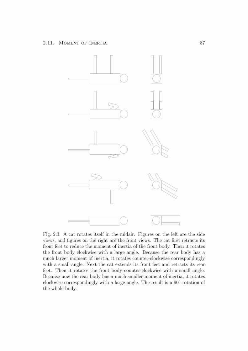
2.11. Moment of Inertia 87
Fig. 2.3: A cat rotates itself in the midair. Figures on the left are the sideviews, and figures on the right are the front views. The cat first retracts itsfront feet to reduce the moment of inertia of the front body. Then it rotatesthe front body clockwise with a large angle. Because the rear body has amuch larger moment of inertia, it rotates counter-clockwise correspondinglywith a small angle. Next the cat extends its front feet and retracts its rearfeet. Then it rotates the front body counter-clockwise with a small angle.Because now the rear body has a much smaller moment of inertia, it rotatesclockwise correspondingly with a large angle. The result is a 90 rotation ofthe whole body.

88 Chapter 2. Motion of Particles
where α is the particle label. If the center of mass is located at b, the positionvector with respect to the center of mass is
r′ = r− b. (2.62)
With respect to the center of mass, the moment-of-inertia tensor is
I ′ij =∑α
mαδij|rα − b|2 − [(rα − b) · ei][(rα − b) · ej]
=∑α
mα[δijr2α − (rα · ei)(rα · ej)]
+∑α
mα[−δij2rα · b + (rα · ei)(b · ej) + (b · ei)(rα · ej)]
+∑α
mα[δijb2 − (b · ei)(b · ej)]. (2.63)
Because∑α
mαrα = Mb, (2.64)
where M =∑
α mα, the second term on the right-hand side of Eq. (2.63) issimply −2 times the third term. Hence we have
I ′ij = Iij −M [δijb2 − (b · ei)(b · ej)]. (2.65)
The second term on the right-hand-side is simply the moment of inertia of aparticle of mass M at location b. Eq. (2.65) is known as the parallel axistheorem for moment of inertia.
In Eq. (2.31) we have already shown how a vector transforms under rota-tion. If we rotate the coordinate frame instead of the vector itself, the vectortransforms the same way as in Eq. (2.31), except that we reverse the anglesξ, φ, and ψ. The transformation matrix S = T1(−ξ)T2(−ψ)T3(−ψ) satisfiesthe unitary condition S† = S−1. Let us investigate how Iij transforms underthe rotation of the coordinate frame. By Eq. (2.54), in the new coordinateframe we have
I ′ij =∑α
mα
[δijr
′(α)k r
′(α)k − r
′(α)i r
′(α)j
]. (2.66)
Substituting r′(α)i = Sijr
(α)j into Eq. (2.66), we have
I ′ij =∑α
mα
[δijSklr
(α)l Skmr(α)
m − Sjmr(α)m Sikr
(α)k
]
=∑α
mα
[δijr
(α)l S†lkSkmr(α)
m − Sikr(α)k r(α)
m S†mj
]. (2.67)

2.12. The Shell Theorem of Gravity 89
Fig. 2.4: Calculating the gravitational potential from a mass sphere.
Since S†lkSkm = δlm,
I ′ij =∑α
mα
[δijr
(α)l δlmr(α)
m − Sikr(α)k r(α)
m S†mj
]
= δij
(∑α
mαr(α)m r(α)
m
)− Sik
(∑α
mαr(α)k r(α)
m
)S†mj. (2.68)
The first term is already diagonalized, and in Section 1.8 we show that thesecond term can also be diagonalized if we choose the column vectors of S†
to be the eigenvectors of the matrix Mkm =∑
α mαr(α)k r(α)
m . In other words,Iij can always be written as Eq. (2.57) in some coordinate frame.
2.12 The Shell Theorem of Gravity
Consider the gravitational potential field produced by a spherical uniformmass shell of radius R. We shall calculate the potential field at a position rfrom the center of the shell. Let us choose r to be the θ = 0 direction, suchthat the shell can be divided into surface elements 2πR2 sin θdθ as shownin Fig. 2.4. The distances from the surface elements to the position r are√
r2 + R2 − 2rR cos θ. The potential field is
φ(r) = −G∫ π
0
ρ2πR2 sin θ dθ√r2 + R2 − 2rR cos θ
, (2.69)
where ρ is the surface mass density. Let us define y = cos θ and x = r/R.We have
φ(r) = 2πGρR∫ −1
1
dy√x2 + 1− 2xy

90 Chapter 2. Motion of Particles
=2πGρR
−x
√x2 + 1− 2xy
∣∣∣∣y=−1
y=1. (2.70)
If x > 1, the position r is outside of the shell. We have
φ(r) =2πGρR
−x[x + 1− (x− 1)] = −4πGρR
x= −GM
r, (2.71)
where M = 4πρR2 is the total mass of the shell. The potential field is thesame as that produced by a point of mass M at the center of the shell. Ifx < 1, the position r is inside of the shell. We have
φ(r) =2πGρR
−x[x + 1− (1− x)] = −4πGρR = −GM
R. (2.72)
In this case the potential is a constant. Therefore there is no gravitationalforce in the shell.
2.13 The Kepler Problem
Let us now discuss the Kepler’s laws in terms of Newton’s law of universalgravitation. In the 17th century, Kepler wrote down three empirical lawsbased on his analysis of observational data on the motion of planets. Thelaws are:
1. Planets move in elliptical obits, with the Sun at one of the foci.
2. A line connecting a planet and the Sun sweeps out an area at a constantrate.
3. The square of the obit period is proportional to the third power of theplanet’s average distance from the Sun.
The great success of Newton’s law of universal gravitation is that Kepler’slaws can be derived completely from it.
Let us consider a general central force f(r). The equation of motion is
p = f(r)r
r, (2.73)
2.13. The Kepler Problem 91
where in our notation r = |r|. The angular momentum follows the followingequation
L =d
dt(r× p) = r× p + r× p
= r×mr + r× f(r)r
r= 0, (2.74)
hence is a constant vector. The cross product of p with the constant angularmomentum L can be expanded as
p× L = f(r)r
r×m(r× r) =
mf(r)
r[r× (r× r)]
=mf(r)
r[r(r · r)− r2r]. (2.75)
Since
r · r =1
2
d
dt(r · r) = rr, (2.76)
we may replace r · r in Eq. (2.75) by rr to obtain
d
dt(p× L) = −mf(r)r2
(r
r− rr
r2
)(2.77)
= −mf(r)r2 d
dt
(r
r
). (2.78)
Substituting in the force of gravity f(r) = −k/r2, we can define
A ≡ p× L−mkr
r, (2.79)
and immediately we see A = 0, namely A is a conserved vector like theangular momentum. It is known as the Laplace-Runge-Lenz vector. Themagnitude of A can be derived from
A ·A =(p× L−mk
r
r
)·(p× L−mk
r
r
)
= (p× L) · (p× L)− 2mk
rr · (p× L) + m2k2. (2.80)
Using the formula (a×b) · (c×d) = (a · c)(b ·d)− (a ·d)(b · c), and notingthat
r · (p× L) = L · (r× p) = L2, (2.81)

92 Chapter 2. Motion of Particles
Eq. (2.80) can be reduced to
A ·A = p2L2 − 2mk
rL · (r× p) + m2k2
= 2mL2
(p2
2m− k
r
)+ m2k2
= 2mL2E + m2k2, (2.82)
where E is the total energy of the system.
From the definition of A, it is clear that
A · L = 0, (2.83)
Therefore A must be a fixed vector lying in the plane of planet motion. Letthe direction of A be the θ = 0 axis in the polar coordinate system. We have
r ·A = Ar cos θ = r · (p× L)−mkr. (2.84)
From Eq. (2.81), Eq. (2.84) is
Ar cos θ = L2 −mkr. (2.85)
Writing Eq. (2.85) in rectangular coordinates, we have
x2 + y2 =
(L2 − Ax
mk
)2
, (2.86)
or(
1− A2
m2k2
) [x +
L2A/(m2k2)
1− A2/(m2k2)
]2
+ y2 =L4/(m2k2)
1− A2/(m2k2). (2.87)
Set
a2 =L4/(m2k2)
[1− A2/(m2k2)]2=
k2
4E2, (2.88)
b2 =L4/(m2k2)
1− A2/(m2k2)=
L2
−2mE, (2.89)
c =L2A/(m2k2)
1− A2/(m2k2)=
A
−2mE, (2.90)
then
(x + c)2
a2+
y2
b2= 1. (2.91)

2.13. The Kepler Problem 93
From Eq. (2.82) and Eqs.(2.88)–(2.90), it can be seen that a2 − b2 = c2,therefore the origin (0, 0) is one of the foci. If E < 0, the planet is boundedby the gravity. In this case both a2 and b2 are positive and Eq. (2.91) is theequation for an ellipse, which gives Kepler’s first law. For the unbound casewe have E > 0, then a2 is still positive but b2 becomes negative, and thetrajectory is a hyperbola. Eqs. (2.82) and (2.91) yield
(4E
k2
)x2 −
(4A
mk2
)x−
(2m
L2
)y2 = −
(2L2
mk2
). (2.92)
If E → 0, we have the critically bounded case in which Eq. (2.92) reduces to
(4
k
)x +
(2m
L2
)y2 =
(2L2
mk2
), (2.93)
or
y2 = −2L2
mk
(x− L2
2mk
). (2.94)
This is a parabola with the focus at the origin.
Conservation of the angular momentum means
m
∣∣∣∣∣r×dr
dt
∣∣∣∣∣ = L = constant. (2.95)
Because |r× dr| is the area spanned by r and dr, we see the vector r sweepsan area with a constant rate. This is Kepler’s second law. Let us integratethe area S(t) swept by the vector r for one period T .
S(T ) =∫ T
0
1
2
∣∣∣∣∣r×dr
dt
∣∣∣∣∣ dt (2.96)
=LT
2m= πab. (2.97)
Substituting in the expressions for a and b in Eqs. (2.88) and (2.89), we have
T =2mπab
L=
2πL3/(mk2)
[1− A2/(m2k2)]3/2= 2π
√m
ka3/2
=2π√GM
a3/2. (2.98)
Since in an ellipse the sum of the distances to the two foci is 2a, the averagedistance to one of the focus is a. Eq. (2.98) gives Kepler’s third law.

94 Chapter 2. Motion of Particles
Fig. 2.5: A rod hanging on a wall.
2.14 Exercises
Exercise 2.1. A fish can swim at a speed of 3 m/s on still water. It wantsto cross a river while spending the shortest possible time. In what directionshould it go with respect to the bank if the speed of water is (1) 2 m/s, (2)4 m/s? Assume that the speed of the water is the same everywhere.
Exercise 2.2. A fish can swim at a speed of 3 m/s on still water. It wants tocross a river while traveling the shortest possible distance. In what directionshould it go with respect to the bank if the speed of water is (1) 2 m/s, (2)4 m/s? Assume that the speed of the water is the same everywhere.
Exercise 2.3. A rod of mass m is hanging on the wall as shown in Fig. 2.5.One end of the rod is pulled by a string fixed to the wall at point A, andthe other end is pushed against the wall at point B by gravity. The distancebetween A and B is equal to the length of the rod, and the angle betweenthe rod and the wall is θ. If the force exerted by the wall to the rod at pointB is F, what is |F| as a function of θ?
Exercise 2.4. A spring with a uniform mass density ρ has a spring constantk. When the spring is placed horizontally on a table without being stretched,its length is L. What is its length when it is hung vertically and stretchedby the gravitational force? Note that when the spring is hung vertically, itsmass density is no longer uniform, because the upper part is stretched morethan the lower part.
Exercise 2.5. A fishing boat had lost its direction on a foggy sea. Thecaptain decided to sail in a fixed direction at a constant speed vt in the

2.14. Exercises 95
hope that the boat would eventually reach the shore. At the same time,he reported to the police through radio the position of the boat and thespeed and direction of sailing. However, the radio broke down during thetransmission, so that the police only knew the position and the speed, not thedirection. Nevertheless, a speedboat capable of sailing at vp was dispatchedto search for this fishing boat. When the speedboat arrived at the reportedposition, a time ∆t had passed. Because the police did not know in whatdirection the fishing boat went, it seemed that there was no way to continue.However, because the captain of the speedboat learned calculus well, hefigured out a reliable plan to catch the fishing boat. If you were the captain,what would be your plan? How long would it take? What was the distancethe speedboat traveled before catching the fishing boat? Note that since youdo not know the moving direction of the fishing boat, there may be someparameters of random choice in your plan. The answer will of course dependon these parameters, instead of being a fixed number.
Exercise 2.6. There are four ants in the four corners of a square room oflength l. Ant A is at the south-east corner, ant B is at the north-east corner,ant C is at the north-west corner, and ant D is at the south-west corner.Starting at t = 0, ant A moves toward its target ant B, ant B moves towardits target ant C, ant C moves toward its target ant D, and ant D movestoward its target ant A. All the ants move at a fixed speed v in the directionpointing to their respective targets. Eventually, the four ants collide in thecenter of the room. How far has each ant traveled? How long does it take?What are the coordinates of ant A as functions of time? (Hint: If you use thereal time t as the variable for the equation of motion, the equation becomeshighly nonlinear. Choose a suitable variable s, which is a function of t, toreduce the equation of motion to a linear form. You do not need to knows(t) explicitly to begin with; you only need to define s through a relationbetween ds and dt, namely ds/dt = f(t). Neither do you need to know whatis f(t) in the beginning. After the problem is solved in the variable s, f(t)will become obvious.)
Exercise 2.7. Landslide can occur if the coefficient of static friction µs
between soil is reduced by heavy rain. For a 45 slope, what is the minimumvalue of µs before landslide occurs?
Exercise 2.8. Two identical balls A and B are in contact with each other.Their centers are on the y-axis and the contact point is at the origin. Athird identical ball C moving at a speed of 10 m/s along the x-axis collideselastically with A and B. Find the velocities of all three balls after collision.
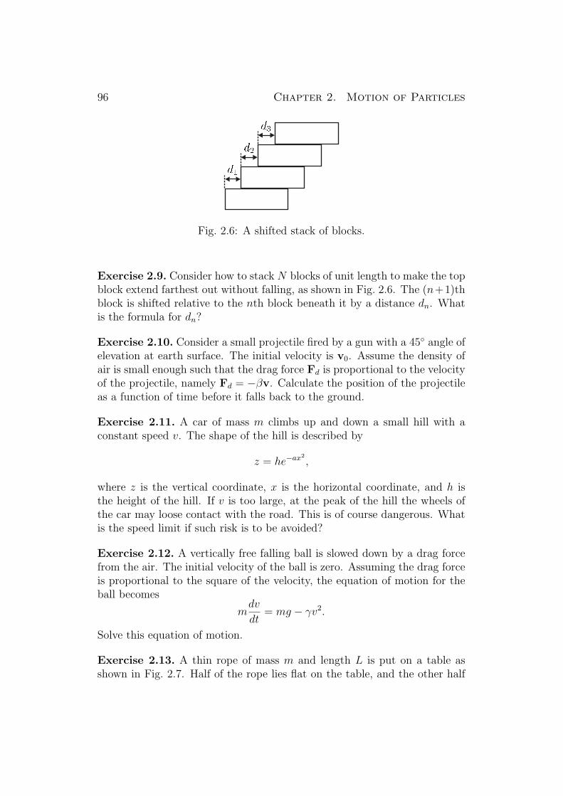
96 Chapter 2. Motion of Particles
Fig. 2.6: A shifted stack of blocks.
Exercise 2.9. Consider how to stack N blocks of unit length to make the topblock extend farthest out without falling, as shown in Fig. 2.6. The (n+1)thblock is shifted relative to the nth block beneath it by a distance dn. Whatis the formula for dn?
Exercise 2.10. Consider a small projectile fired by a gun with a 45 angle ofelevation at earth surface. The initial velocity is v0. Assume the density ofair is small enough such that the drag force Fd is proportional to the velocityof the projectile, namely Fd = −βv. Calculate the position of the projectileas a function of time before it falls back to the ground.
Exercise 2.11. A car of mass m climbs up and down a small hill with aconstant speed v. The shape of the hill is described by
z = he−ax2
,
where z is the vertical coordinate, x is the horizontal coordinate, and h isthe height of the hill. If v is too large, at the peak of the hill the wheels ofthe car may loose contact with the road. This is of course dangerous. Whatis the speed limit if such risk is to be avoided?
Exercise 2.12. A vertically free falling ball is slowed down by a drag forcefrom the air. The initial velocity of the ball is zero. Assuming the drag forceis proportional to the square of the velocity, the equation of motion for theball becomes
mdv
dt= mg − γv2.
Solve this equation of motion.
Exercise 2.13. A thin rope of mass m and length L is put on a table asshown in Fig. 2.7. Half of the rope lies flat on the table, and the other half

2.14. Exercises 97
Fig. 2.7: A rope falling from a table.
hangs vertically through a hole near the edge. As gravity pulls the ropedown, what is the position of the center of the rope relative to the table asa function of time? Assume there is no friction between the rope and thetable.
Exercise 2.14. A bicycle is constructed in such a way that the radius ofthe wheels is 30 cm and the distance between the axes of the wheels is 1 m.When a 60-kg rider is riding the bicycle on flat ground, the center of massfor the rider and the bicycle as a whole is at equal distance from the axes ofthe wheels and at a height of 60 cm from the ground. After a while the riderencounters a 30 down slope. As the bicycle goes down the slope it picksup a speed of 40 km/hr. At this moment the rider decides to pull the frontbreak. This is of course dangerous, because the bicycle may turn over. Atwhat deceleration, the rear wheel starts to loose contact with the ground?
Exercise 2.15. An observer on the Earth finds a motionless uniform ropehanging vertically from the sky. One end of the rope is just above the ground,and the other end extends high up into the sky beyond the visual range. If hehad not learned physics, he might think the rope is hanging from a spaceshipsent by extra-terrestrial beings. However, it is possible for a bare rope to hangfrom the space just like the Moon hangs on the sky. How long should therope be? In this exercise we assume the Earth does not have an atmosphere.
Exercise 2.16. A transparent vacuum tunnel was built to test a magnetic-

98 Chapter 2. Motion of Particles
levitated prototype train powered by hydrogen fuel cells. Peter, who wasstanding by the tunnel, observed that at the first stage the train used x litersof fuel to accelerate from 0 to 100 km/hr, and at the second stage the trainused 3x liters more of fuel to accelerate from 100 to 200 km/hr. Because themotion of the train has almost no friction, Peter figured that all the energyof the fuel was converted to the kinetic energy of the train. That is why inthe first stage the fuel consumption was x liters while in the second stagethe fuel consumption was 3x liters. Another observer Paul, who was on anordinary train moving at a speed of 100 km/hr in the opposite direction, alsowitnessed the event. From his point of view, in the first stage the speed of theprototype train increased from 100 to 200 km/hr, while in the second stagethe speed increased from 200 to 300 km/hr. Therefore Paul figured in thesecond stage the fuel consumption should be (32 − 22)/(22 − 12)x = (5/3)xliters. Who is right, Peter or Paul? If one is right, the other must have madea mistake in his calculation. Do the correct calculation for the wrong one.
Exercise 2.17. A sniper at a latitude of 30 north is aiming at a small target1 km away in the north. The speed of the bullet is 800 m/s. If the sniperdoes not take into account the rotation of the Earth, by how far to the eastor the west will the bullet miss the target? In this exercise we assume theEarth does not have an atmosphere.
Exercise 2.18. A powerful rail gun located at the Equator is aimed at thehorizontal direction toward east. With the aid from the spin of the Earth,the gun is capable of launching a projectile to the escape velocity of theEarth, so that the projectile has just enough energy to break loose fromthe gravitational pull of the Earth and travel to a place that is infinitelyfar away. Because the spin of the Earth adds velocity to the projectile,when the gun is placed at the Equator and aimed at the horizontal directiontoward east minimum energy from the power supply of the gun is required.However, because of a mistake in the calculation, the energy stored into thepower supply of the gun is only 95% of this minimum energy. Assumingall the energy stored into the power supply of the gun is converted to thekinetic energy of the projectile, how long after the launch will the projectilereturn to the Earth? In this exercise we assume the Earth does not have anatmosphere. We also ignore the influence from the Moon, the Sun, and otherplanets.
Exercise 2.19. A dumb-bell sits on a horizontal frictionless table, not mov-ing or rotating, as shown in Fig. 2.8. The dumb-bell can be considered astwo point masses M joined by a massless rod of length L. A ball of mass

2.14. Exercises 99
Fig. 2.8: A dumb-bell hit by a ball.
Fig. 2.9: Falling into a mine.
m < M moving in the −x direction with velocity v makes a head-on elasticcollision with one of the mass point of the dumb-bell and bounces back inthe x-direction. After the collision, what is the center-of-mass motion andthe rotational motion of the dumb-bell? What is the velocity of the ball afterthe collision?
Exercise 2.20. A crazy mining company has dug up a tunnel from thesurface of the Earth all the way down to the center of the Earth. At themidpoint of the tunnel it has dug up a spherical cavity of radius R/4, whereR is the radius of the Earth, as shown in Fig. 2.9. An unfortunate workerfalls into the tunnel. What is the impact velocity when the worker hits theend of the tunnel? In this exercise we assume the Earth does not have anatmosphere.
Exercise 2.21. The mass of Jupiter is 1.9× 1027 kg and its speed relative tothe Sun is 13 km/s. A spacecraft of 3000 kg approaches Jupiter with a speedof 3 km/s relative to the Sun. The trajectory of the spacecraft is bent by

100 Chapter 2. Motion of Particles
the gravitational force from Jupiter such that in a reference frame fixed toJupiter the spacecraft comes in with a velocity v and leaves with a velocity u.The angle between v and u is θ. Show that the final speed of the spacecraftrelative to the Sun after this soft encounter can be much larger than its initialvelocity 3 km/s. Find the final speed of the spacecraft as a function of θ.
Exercise 2.22. On the line connecting the Earth and the Sun there is a pointrotating with the same angular velocity as that of the Earth around the Sun,where the gravitational forces from the Earth and the Sun and the centrifugalforce cancel each other. This is called the first Lagrange point. How far isthis point from the center of the Earth? Give a numerical answer. Considerthe shape of the effective potential function at this point in a rotating framein which the origin is at the center of the Sun and the position vector of theEarth is r. The frame rotates with the same angular velocity as that of theEarth around the Sun. Does the potential function has a minimum in ther-direction? Does the potential function has a minimum in the θ-direction(the direction perpendicular to r)? Hint: Define α ≡ m/M ¿ 1, where m isthe mass of the Earth and M the mass of the Sun, and β ≡ l/L, where l isthe distance from the Earth to the first Lagrange point and L the distancefrom the Earth to the Sun. Write the equilibrium condition in terms of α andβ. Assuming β ¿ 1 for the time being, one can throw away high-order termsof both α and β to simplify the equation. After solving the equation, verifyβ ¿ 1 for consistency. How many terms to throw away is your own choice.Here we only ask for a numerical answer that is accurate to the second digit.
Exercise 2.23. Consider a base-ball bat shown in Fig. 2.10. Point c is thecenter of mass. Point a is the position to hold the bat when striking. If thebat is pivoted about a horizontal frictionless axis through a to form a physicalpendulum, its frequency of small oscillation is ω. Point b is chosen such thatif the bat is pivoted about a horizontal frictionless axis through b to form aphysical pendulum, its frequency of small oscillation is also ω. Show that,if the hitter strikes the base ball at b with the velocity of the incoming ballperpendicular to the axis of the bat, his hands at a do not feel the reactionforce. In this problem we assume the surface of the bat around point b iscylindrical and it is parallel to the axis of the bat. Hint: If the strike point isat c, then the bat will recoil back without rotation. In contrast, if the strikepoint is at the opposite end of a from c, the bat tends to rotate in addition torecoiling back. If the strike point is far enough from c, the rotation can makepoint a move in the opposite direction of the incoming base ball. Hence inbetween there is an ideal strike point for which a does not move.

2.14. Exercises 101
Fig. 2.10: The best point to strike a base ball.
Fig. 2.11: Tilting a rotating ball.
Exercise 2.24. A solid ball of mass m and radius r is rotating around ahorizontal shaft parallel to the x-axis. The angular velocity is ωx whereω > 0. The shaft is supported by two vertical poles that are parallel to thez-axis and separated by a distance d. The ball is at an equal distance d/2from the poles. If the shaft is tilted by a small angle θ ¿ 1 as shown inFig. 2.11, what is the impulse acted on each pole? Note that impulse is anvector, so you should include the direction of the impulse in your answer.
Exercise 2.25. Consider a particle moving in the x-y plane under the grav-itational force from a massive thin wire in the z-axis. The wire extends fromz = −∞ to z = ∞. The mass per unit length is ρ. Show that for any initialposition and initial velocity, it is not possible to escape from this gravitationalsystem. As usual, here “escape” means to go as far as one wants.
Exercise 2.26. In the outer space there is a uniform massive thin shell ofradius R with a small round opening of radius r ¿ R on the top. The massper unit area of the shell is ρ. A particle is released at the center of the

102 Chapter 2. Motion of Particles
shell with zero initial velocity. What is the final velocity of the particle as itcollides with the shell?
Exercise 2.27. Oil companies search underground pocket of oil by detectingthe minute change of gravitational force at the Earth surface. Assume thedetector is right above an underground spherical pocket of oil. The radius ofthe pocket is r and the center of the pocket is at a depth d. If the change ofgravitational acceleration can be written as
∆g = g − g0 = a− bx2,
where g0 = 9.8 m/s2 and x is a small horizontal displacement of the detectorfrom the position right above the pocket at the Earth surface, what is r andd in terms of a and b? In this problem we assume the Earth is a uniformsolid sphere of density ρe without spin and the oil has a uniform density ρo.Note that we assume x ¿ r < d and d ¿ R, where R is the radius of theEarth.
Exercise 2.28. A 10-g marble is launched vertically by a sling-shot with aninitial velocity of 20 m/s. Assume the drag force F from the air is given byF = γv2, where v is the velocity of marble and γ = 8 × 10⁻⁵ kg/m. Howlong does it take for the marble to reach the maximum height? What is themaximum height? In this problem we assume the Earth has no spin.
Exercise 2.29. A roller coaster runs with a constant speed v along a trackdescribed by h(x) = h0(tanh x+1), where h is the height of the track, x is thehorizontal coordinate, and h0 is a constant. During a run from x = −100 tox = 100, the maximum acceleration experienced by the roller coaster is amax.If in the next run the speed is changed to 2v, what will be the maximumacceleration?
Exercise 2.30. A top is made of a solid ball attached to a pin of negligiblemass. The mass of the ball is 0.25 kg and the radius is 2 cm. The topis spinning at a rate of 1200 rpm. The the distance between center of thesphere and the end of the pin, where the top is supported, is 4 cm. The anglebetween the top’s rotation axis and the vertical axis is 15. Due to the torqueproduced by the gravitational force, the angular momentum rotates slowlyaround the vertical axis, as shown in Fig. 2.12. This rotation is known as thegyroscopic precession. What is the rate of precession? In your calculationdoes the precession change the angle between the angular momentum andthe vertical axis? If not, how can a top fall eventually as it slows down?
Exercise 2.31. A short section of round pipe made of honeycomb composite
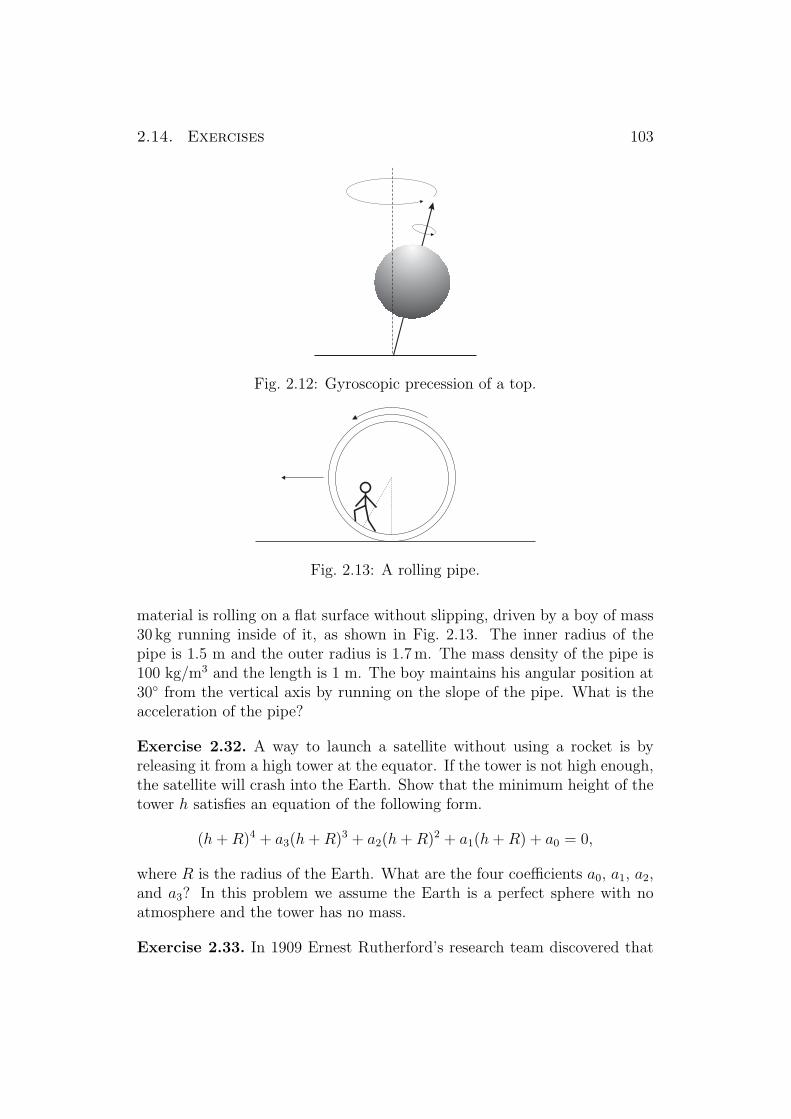
2.14. Exercises 103
Fig. 2.12: Gyroscopic precession of a top.
Fig. 2.13: A rolling pipe.
material is rolling on a flat surface without slipping, driven by a boy of mass30 kg running inside of it, as shown in Fig. 2.13. The inner radius of thepipe is 1.5 m and the outer radius is 1.7 m. The mass density of the pipe is100 kg/m3 and the length is 1 m. The boy maintains his angular position at30 from the vertical axis by running on the slope of the pipe. What is theacceleration of the pipe?
Exercise 2.32. A way to launch a satellite without using a rocket is byreleasing it from a high tower at the equator. If the tower is not high enough,the satellite will crash into the Earth. Show that the minimum height of thetower h satisfies an equation of the following form.
(h + R)4 + a3(h + R)3 + a2(h + R)2 + a1(h + R) + a0 = 0,
where R is the radius of the Earth. What are the four coefficients a0, a1, a2,and a3? In this problem we assume the Earth is a perfect sphere with noatmosphere and the tower has no mass.
Exercise 2.33. In 1909 Ernest Rutherford’s research team discovered that

104 Chapter 2. Motion of Particles
the scattering angle of an alpha particle by gold foil can be unexpectedlylarge. This led to the postulate that atoms have a highly concentrated nucleusthat contains all the positive charges. Considering an alpha particle flyingtoward a gold nucleus with a velocity of 1.8×10⁷ m/s. The Coulomb repulsiveforce will bend the trajectory, such that the alpha particle will leave the goldnucleus at an angle θ with respect to the incoming direction. Let d be thesmallest distance between the alpha particle and the gold nucleus during theencounter. As one can imagine, a smaller d yields a larger θ. If θ = 90,how small is d? In this problem we assume the mass ratio between the alphaparticle and the gold nucleus is zero, such that the gold nucleus does notmove. We also assume that the electrons around the gold nucleus have noeffect on the alpha particle because they are evenly distributed in a muchlarger space. Note that the atomic number of gold is 79.

Chapter 3
Oscillators and Waves
3.1 Driven Harmonic Oscillators
An ideal simple harmonic oscillator can oscillate indefinitely. However, inreality there is always some friction that damps the oscillation. Thereforecontinuous oscillation must be driven by external forces. The equation ofmotion for a driven harmonic oscillator with damping is
mx + µx + kx = F (t), (3.1)
where −µx represents the damping force, −kx the restoring force, and F (t)the external driving force. It is more convenient to use the following form
x + γx + ω20x = f(t), (3.2)
where γ = µ/m and f(t) = F (t)/m. First, let us consider the case in whichf(t) = 0. The solutions are
x(t) = a1eλ+t + a2e
λ−t, (3.3)
where a1 and a2 are determined by the initial conditions, and
λ± =−γ ±
√γ2 − 4ω2
0
2. (3.4)
If γ > 2ω0, the oscillator is called an overdamped oscillator. The solutionsare just exponentially decaying functions, and there is no oscillation at all.
105
106 Chapter 3. Oscillators and Waves
If γ < 2ω0, the oscillator is called an underdamped oscillator. It oscillates
at a frequency ω =√
ω20 − γ2/4 with an exponentially decaying amplitude
e−γt/2. If we choose the coefficients in Eq. (3.3) to be a1 = a2 = b1/2 ora1 = −a2 = b2/(2i), the two solutions for an underdamped oscillator can beexpressed as
x(t) = b1e−γt/2 cos ωt (3.5)
or
x(t) = b2e−γt/2 sin ωt. (3.6)
If γ = 2ω0, the oscillator is called a critically damped oscillator. In this casethe two independent solutions can be found by taking the limit of ω → 0 inEqs. (3.5) and (3.6) regardless of the constant coefficients in front of them,which will be determined by the initial condition anyway. Hence the solutionsfor a critically damped oscillator are e−ω0t and te−ω0t.
Next, let us assume f(t) is nonzero only between t = 0 and t = T . Weneed to find a special solution to add to the solutions in Eq. (3.3). Let uswrite x(t) and f(t) in terms of their Fourier transforms.
x(t) =1√2π
∫ ∞
−∞x(ω)eiωtdω, (3.7)
f(t) =1√2π
∫ ∞
−∞f(ω)eiωtdω. (3.8)
Both x(t) and f(t) can be thought of as a superposition of many frequencycomponents cos ωt and sin ωt, and x(ω) and f(ω) represent the amplitude ofthe ω-component. Substituting Eqs. (3.7) and (3.8) into Eq. (3.2). We have
∫ ∞
−∞(−ω2 + iγω + ω2
0)x(ω)eiωtdω =∫ ∞
−∞f(ω)eiωtdω. (3.9)
Comparing both sides, we obtain
x(ω) =f(ω)
−ω2 + iγω + ω20
. (3.10)
Now that we know x(ω), we can calculate x(t) by the inverse Fourier trans-form. Alternatively we may use the convolution theorem of Fourier transformand Eq. (1.254) to obtain
x(t) =1
β
∫ t
−∞f(t′)e−γ(t−t′)/2 sin[β(t− t′)] dt′, (3.11)

3.1. Driven Harmonic Oscillators 107
where
β =
√ω2
0 −γ2
4. (3.12)
In Eq. (3.11), the displacement x(t) at time t can be interpreted as the linearresponse to the external force f(t′) at time t′. Since the response is notinstantaneous, x(t) is a linear combination of all the f(t′) with coefficient1βe−γ(t−t′)/2 sin[β(t− t′)]. The function g(t) that satisfies the equation
x(t) =∫ ∞
−∞f(t′)g(t− t′) dt (3.13)
is known as the Green’s function. By setting f(t′) = δ(t′) in Eq. (3.13), itcan be seen that the Green’s function g(t) is the solution of the equation
x + γx + ω20x = δ(t). (3.14)
The solution in Eq. (3.11) shows that
g(t) =
1βe−γt/2 sin βt when t ≥ 0
0 when t < 0.(3.15)
For the special case where
f(t) = A cos ωt
=A
2eiωt +
A
2e−iωt, (3.16)
we may assume the solution has the following form:
x(t) = Beiωt + B∗e−iωt. (3.17)
Substituting into Eq. (3.2), we obtain
B =A/2
−ω2 + iγω + ω20
. (3.18)
Set
1
−ω2 + iγω + ω20
= |χ|eiφ, (3.19)
where
|χ| =1
| − ω2 + iγω + ω20|
,
eiφ =| − ω2 + iγω + ω2
0|−ω2 + iγω + ω2
0
, (3.20)

108 Chapter 3. Oscillators and Waves
one obtains
x(t) =A
2
(|χ|eiφeiωt + |χ|e−iφe−iωt
)
= A|χ| cos(ωt + φ). (3.21)
When the driving frequency ω is much smaller than the resonance frequencyω0, we have φ → 0, which shows the oscillator is in phase with the drivingforce. When the driving frequency ω is equal to the resonance frequency ω0,we have φ = −π/2, which shows the oscillator is delayed by 90 degreeswith respect to the driving force. When the driving frequency ω is muchlarger than the resonance frequency ω0, we have φ → −π, which shows theoscillator is out of phase with the driving force.
If the oscillator is weakly damped, γ ¿ ω0. Then x(ω) has a resonancepeak at ω = ω0. Near the resonance peak, ω2
0 − ω2 ≈ 2ω(ω0 − ω), we have
x(ω) ≈ f(ω)/(2ω)
ω0 − ω + iγ/2, (3.22)
and
|x(ω)|2 ≈ |f(ω)|2/(4ω2)
(ω0 − ω)2 + γ2/4. (3.23)
If we define the width of the resonance peak to be the difference between thetwo values of ω that reduce |x(ω)|2 by half, then the width is γ.
Let us go back to see what trick the Fourier transform does to the equa-tion that allows us to get the solution without much effort. In the timedomain Eq. (3.2) is a differential equation. Fourier transform turns it into analgebraic equation in the frequency domain, Eq. (3.10), which is much easierto solve. This is why spectral analysis by Fourier transform is a powerfultool for linear differential equations.
3.2 Harmonic Generation in Nonlinear Oscillators
Consider a particle in a potential well V (x). The equation of motion is
mx = −dV
dx. (3.24)

3.2. Harmonic Generation in Nonlinear Oscillators 109
If we assume that V (x) = V (−x) and the minimum of V (x) is at x = 0, wemay expand V (x) in Taylor series.
V (x) = V (0) +V ′′(0)
2x2 +
V (4)(0)
24x4 + · · · . (3.25)
For small oscillation, namely the motion of the particle is not far from x = 0,the equation of motion is approximately
x = −ω20x− αx3, (3.26)
where ω20 = k/m = V ′′(0)/m and α = V (4)(0)/(6m). If αx3 is omitted, we
get the simple harmonic oscillator. Therefore if the amplitude of oscillation issmall enough such that αx3 ¿ ω2
0x, we should obtain a solution that is onlyslightly different from the solution of the simple harmonic oscillator. Nowlet us see how αx3 changes the solution of the simple harmonic oscillator.Assuming the initial conditions are x(0) 6= 0 and x′(0) = 0, let us try thefollowing function as the first-order guess.
x(t) = a1 cos(ωt) + a3 cos(3ωt). (3.27)
Because the solution should be close to the simple harmonic oscillator, weassume a3 ¿ a1. Substituting it into Eq. (3.26), we obtain
(−a1ω
2 + a1ω20 +
3
4αa3
1 +3
4αa2
1a3 +3
2αa1a
23
)cos(ωt)
+(−a39ω
2 + a3ω20 +
1
4αa3
1 +3
2αa2
1a3 +3
4αa3
3
)cos(3ωt)
+(
3
4αa2
1a3 +3
4αa1a
23
)cos(5ωt)
+3
4αa1a
23 cos(7ωt) +
1
4αa3
3 cos(9ωt) = 0. (3.28)
Since we assume a3 ¿ a1, the coefficient of cos(ωt) gives
ω2 ≈ ω20 +
3
4αa2
1, (3.29)
and the coefficient of cos(3ωt) gives
a3 =14αa3
1
9ω2 − ω20 − 3
2αa2
1
≈14αa3
1
8ω20 + 21
4αa2
1
. (3.30)
Because for small oscillation αa21 ¿ ω2
0,
a3
a1
≈ αa21
32ω20
. (3.31)

110 Chapter 3. Oscillators and Waves
Here we see indeed a3 ¿ a1, which is consistent with our assumption in thebeginning. Note that a3 is proportional to the first order of α. If we keepterms only up to the first order of α, we can ignore the cos(5ωt), cos(7ωt)and cos(9ωt) terms. Therefore Eq. (3.27) is only an approximation up tothe first order of α. We can improve the approximation by adding a terma5 cos(5ωt) to our guess solution, then we will be able to obtain solutions upto the second order of α, only with more complicated calculation.
Eq. (3.29) tells us how the frequency of the nonlinear oscillator changeswith its amplitude, and Eq. (3.30) gives the amplitude of the third harmonicgenerated from the nonlinear term. The oscillation speeds up for positive αand vice versa as expected. The ratio of the third harmonic power to thefundamental power is proportional to the square of the fundamental power,namely
a23
a21
∝ a41. (3.32)
This means the fraction of harmonic distortion of the oscillator increasesquadratically with the fundamental power.
Let us look back at the process we employed to obtain the approximatesolution. The αx3 term in the equation of motion can be thought of as afrequency mixer. Let x(t) = cos(ω1t) + cos(ω2t). The αx3 term will gener-ate terms of frequencies 3ω1, 3ω2, 2ω2 ± ω1, and 2ω1 ± ω2 with amplitudesproportional to α. If we start from the solution of the harmonic oscillatorx(t) = a1 cos(ωt), the αx3 term will generate a term αa3
1 cos(3ωt)/4. There-fore we must add to the solution a term proportional to cos(3ωt) to cancelit. Let the added term be a3 cos(3ωt). The linear response of the added termgives a contribution of (9ω2 − ω2
0)a3 cos(3ωt). Therefore
a3 =αa3
1/4
9ω2 − ω20
≈ αa31
32ω20
. (3.33)
Now that we have the cos(3ωt) term in the solution, mixing the cos(ωt) termand the cos(3ωt) by αx3 leads to the cos(5ωt) term. Because the cos(3ωt)term is proportional to α, the cos(5ωt) term is proportional to α2. Con-tinuing this process, we find the solution contains an infinite sequence ofodd harmonics cos[(2n + 1)ωt] with decreasing amplitudes proportional toαna2n+1
1 /ω2n0 . In this process, x = −ω2
0x is called the zeroth-order equationand a1 cos(ωt) the zeroth-order solution. The term αx3 is called the per-turbation term of the zeroth-order equation. We add a first-order solution
3.2. Harmonic Generation in Nonlinear Oscillators 111
a3 cos(3ωt) to cancel the terms generated from the zeroth-order solution bythe perturbation term of the equation of motion. But the first-order solutiontogether with the zeroth-order solution generate again new terms throughthe perturbation term of the equation of motion. Therefore we have to add asecond-order term to cancel them. If the perturbation term is small enough,correction for each order will be smaller than that for the previous order.The process will converge, and we can have an approximate solution as closeto the real solution as we want. Such a procedure of finding approximatesolutions is known as the perturbation expansion.
Next we consider a weakly damped asymmetric nonlinear oscillator drivenby an external force mf(t) = mA cos(ωt). Any initial oscillation that is notdriven by the external force will be damped out in the long run, thereforewe look for the steady state solution in which the oscillation amplitude doesnot change with time. Again, for small oscillation the equation of motion isapproximately
x = −γx− ω20x− βx2 + A cos(ωt), (3.34)
where β = V ′′′(0)/(2m). Treating βx2 as the perturbation term, we shall usethe following trial solution.
x(t) = a0 + a1 cos(ωt) + b1 sin(ωt)
+a2 cos(2ωt) + b2 sin(2ωt)
+a3 cos(3ωt) + b3 sin(3ωt), (3.35)
where a2 cos(2ωt)+ b2 sin(2ωt) is the first-order correction, and a3 cos(3ωt)+b3 sin(3ωt) is the second-order correction. Substituting into Eq. (3.34), onehas
a0ω20 + β
(a2
0 +a2
1
2+
b21
2+
a22
2+
b22
2+
a23
2+
b23
2
)
+[−a1ω
2 + γb1ω + a1ω20 + β (2a0a1 + a1a2 + b1b2 + a2a3 + b2b3)− A
]cos(ωt)
+[−b1ω
2 − γa1ω + b1ω20 + β (2a0b1 + a1b2 − b1a2 + a2b3 − b2a3)
]sin(ωt)
+
[−4a2ω
2 + 2γb2ω + a2ω20 + β
(a2
1
2− b2
1
2+ 2a0a2 + a1a3 + b1b3
)]cos(2ωt)
+[−4b2ω
2 − 2γa2ω + b2ω20 + β (2a0b2 + a1b1 + a1b3 − b1a3)
]sin(2ωt)
+[−9a3ω
2 + 3γb3ω + a3ω20 + β (2a0a3 + a1a2 − b1b2)
]cos(3ωt)
+[−9b3ω
2 − 3γa3ω + b3ω20 + β (2a0b3 + a1b2 + b1a2)
]sin(3ωt) = 0. (3.36)

112 Chapter 3. Oscillators and Waves
Let us assume a0 is of the same order as βa21, βb2
1 and an, bn are of the sameorder as βn−1an
1 , βn−1bn
1 . We shall justify these assumptions later. If β issmall we can include only terms of the lowest-order correction. That is
a0(ω20 + βa0) + β
(a2
1
2+
b21
2
)= 0, (3.37)
−a1ω2 + γb1ω + a1ω
20 − A = 0, (3.38)
−b1ω2 − γa1ω + b1ω
20 = 0, (3.39)
−4a2ω2 + 2γb2ω + a2ω
20 + β
(a2
1
2− b2
1
2
)= 0, (3.40)
−4b2ω2 − 2γa2ω + b2ω
20 + βa1b1 = 0, (3.41)
−9a3ω2 + 3γb3ω + a3ω
20 + β (a1a2 − b1b2) = 0, (3.42)
−9b3ω2 − 3γa3ω + b3ω
20 + β (a1b2 + b1a2) = 0. (3.43)
Therefore
a0 = − β(a21 + b2
1)
2(ω20 + βa0)
, (3.44)
a1 =−(ω2 − ω2
0)
γ2ω2 + (ω2 − ω20)
2A, (3.45)
b1 =γω
γ2ω2 + (ω2 − ω20)
2A, (3.46)
a2 = β2a1b1γω +
(a21
2− b21
2
)(4ω2 − ω2
0)
4γ2ω2 + (4ω2 − ω20)
2, (3.47)
b2 = βa1b1(4ω
2 − ω20)− γω (a2
1 − b21)
4γ2ω2 + (4ω2 − ω20)
2, (3.48)
a3 = β3γω (a1b2 + b1a2) + (9ω2 − ω2
0) (a1a2 − b1b2)
9γ2ω2 + (9ω2 − ω20)
2, (3.49)
b3 = β(a1b2 + b1a2) (9ω2 − ω2
0)− 3γω (a1a2 − b1b2)
9γ2ω2 + (9ω2 − ω20)
2. (3.50)
As we can see from the solutions of a0, a1, a2, a3 and b1, b2, b3, indeed ourassumptions that a0 is of the same order as βa2
1, βb21 and an, bn are of the same
order as βn−1an1 , β
n−1bn1 are satisfied. The process can be continued by adding
a next-order correction a4 cos(4ωt)+b4 sin(ωt) to the perturbation expansionEq. (3.34), then a more and more accurate solution can be obtained.

3.3. Normal Modes of Coupled Oscillators 113
Fig. 3.1: Two harmonic oscillators coupled by a spring.
3.3 Normal Modes of Coupled Oscillators
Consider the two harmonic oscillators shown in Fig. 3.1. The equations ofmotion for the two harmonic oscillators are
mx1 = −kx1 − k′(x1 − x2),
mx2 = −kx2 − k′(x2 − x1). (3.51)
Clearly, x1 and x2 are not independent of each other, and the solutions arenot obvious. The equations can be much simplified by choosing another setof variables.
u1 ≡ (x1 + x2),
u2 ≡ (x1 − x2). (3.52)
Then the equations become
mu1 = −ku1,
mu2 = −(k + 2k′)u2. (3.53)
The new set of variables changes the coupled equations into uncoupled ones.Therefore x1+x2 and x1−x2 are the two independent modes of oscillation forthis system of oscillators. Such independent modes of oscillation are knownas normal modes.
3.4 Swinging a Swing
When you were a child, you probably had the experience of playing with aswing. You might have noticed that by moving your body up and down insynchronization with the swing, you could make the amplitude of the swinggrow by yourself, without someone else pushing the swing. In an ideal swing,

114 Chapter 3. Oscillators and Waves
no matter how you change the height of the center of mass of your body, youcan only exert a force in the radial direction, and the force is balanced by thetension of the swing. How can you affect the rotational motion of the swingwithout an external torque? In this section we shall analyze this problem.
Consider an ideal swing in which the player can move his/her center ofmass up and down by a small distance y = y0 cos(Ωt), as shown in Fig. 3.2.The equation of motion is
m(l + y)2θ = −2m(l + y)yθ −mg(l + y)θ, (3.54)
where l is the length of the swing and m is the mass of the player. Thefirst term on the right-hand side is the Coriolis force. Dividing by m(l + y),Eq. (3.54) becomes
(l + y)θ = −2yθ − gθ. (3.55)
Assume the solution we are looking for has the following form:
θ(t) = a(t) cos(ωt) + b(t) sin(ωt), (3.56)
where ω =√
g/l is the resonance frequency of the swing, and a(t), b(t) are
the slow-varying amplitudes. Because a(t) and b(t) vary slowly, a and b arefirst-order small quantities. Remember that we have also assumed y is afirst-order small quantity, therefore a, b, ay, ay, by, and by are all second-order small quantities. Ignoring all the second-order small quantities whensubstituting the trial solution Eq. (3.56) into Eq. (3.55), we obtain
l[−2aω sin(ωt) + 2bω cos(ωt)− aω2 cos(ωt)− bω2 sin(ωt)
]
+y[−aω2 cos(ωt)− bω2 sin(ωt)
]
= −2y [−aω sin(ωt) + bω cos(ωt)]− g[a cos(ωt) + b sin(ωt)]. (3.57)
Since lω2 = g, it is
l[−2aω sin(ωt) + 2bω cos(ωt)
]+ y
[−aω2 cos(ωt)− bω2 sin(ωt)
]
= −2y [−aω sin(ωt) + bω cos(ωt)] . (3.58)
If the swing is driven resonantly, Ω must be an integer multiple of ω. WhenΩ = 2ω, namely y = y0 cos(2ωt), we obtain
[−2aωl +
1
2bω2y0
]sin(ωt) +
[2bωl − 1
2aω2y0
]cos(ωt)
−1
2bω2y0 sin(3ωt)− 1
2aω2y0 cos(3ωt)
= 2bω2y0 sin(ωt)− 2aω2y0 cos(ωt)
+2bω2y0 sin(3ωt) + 2aω2y0 cos(3ωt). (3.59)

3.4. Swinging a Swing 115
Fig. 3.2: A model of an ideal swing.
Both sides of the equation contain the lowest power of cos(ωt) and sin(ωt).Comparing coefficients, we have
a =−3ωy0
4lb, (3.60)
b =−3ωy0
4la. (3.61)
But what about the coefficients of cos(3ωt) and sin(3ωt)? Just like whatwe did in treating the nonlinear oscillators, they can be taken care of byincluding higher-order terms such as a3(t) cos(3ωt) and b3(t) sin(3ωt) in thetrial solution Eq. (3.56). For simplicity, here we work out the lowest-ordersolution first. Combining Eqs. (3.60) and (3.61), one has
a =(
3ωy0
4l
)2
a. (3.62)
Assume y0 > 0 and let λ = 3ωy0/(4l), the solution is then
a(t) = a+eλt + a−e−λt, (3.63)
and from Eq. (3.60)
b(t) = −a+eλt + a−e−λt. (3.64)
The decaying solution associated with a− can be ignored in the long run, andthe growing solution associated with a+ is what we are interested in. Namely
θ(t) = a+[cos(ωt)− sin(ωt)]eλt, (3.65)

116 Chapter 3. Oscillators and Waves
Fig. 3.3: A model of longitudinal mechanical waves.
From the solution we see that in order to make a swing swing, one musthave an initial oscillation first, and the player should raise and lower his/hercenter of mass at twice of the resonant frequency of the swing. When theswing is at an phase angle of π/4, the player should position his/her centerof mass at the lowest point and start to stand up, until the swing is at anphase angle of 3π/4. At this point the player should have the highest centerof mass. Then the player should start to lower down again, until the swingreverse to an phase angle of 5π/4, which is equivalent to π/4 in the reversedirection.
We may now add a correction term a3 cos(3ωt) + b3 sin(3ωt) to θ(t) sothat Eq. (3.55) is satisfied better. This additional term generates
−8lω2[a3 cos(3ωt) + b3 sin(3ωt)] (3.66)
in Eq. (3.55) plus higher order terms in cos(5ωt) and sin(5ωt) as well as smallcorrection terms in cos(ωt) and sin(ωt). To cancel the cos(3ωt) and sin(3ωt)terms, we have
a3 = −ay0
4l,
b3 = −by0
4l. (3.67)
Because y0 ¿ l, the correction term is indeed small compared with a(t)and b(t). To obtain more and more accurate solutions, this process can becontinued by adding correction terms a5 cos(5ωt) + b5 sin(5ωt), a7 cos(7ωt) +b7 sin(7ωt), and so on.
3.5 Waves on a String
In classical mechanics, wave is a simple form of collective motion whoseclosest analogy is vibration. Consider a one-dimensional string of bounded

3.5. Waves on a String 117
particles in which each particle’s motion is influenced by its two nearestneighbors, as shown in Fig. 3.3. If the motion of the particles around itsequilibrium point is small, one can assume the force acting on each particleis proportional to the separation between the particles. The equation ofmotion reads:
mal = η(al−1 − al) + η(al+1 − al), (3.68)
where m is the mass of the particles, al the displacement of the lth particlefrom the equilibrium point, and η the spring constant. Because the string isfixed at both end points (l = 0 and l = N) we have a0(t) = aN(t) = 0. Thissystem of linear equations can be solved by a change of variable (Fouriertransformation)
al(t) =∑
k
uk(t) sin(kls) + vk(t) cos(kls), (3.69)
where s is the distance between neighboring particles. The boundary condi-tion a0(t) = 0 sets vk(t) = 0, and the possible values of k is determined bythe other boundary condition aN(t) = 0, which yields kNs = nπ or kL = nπ,where L is the length of the string and n is a positive integer. Substituting
al(t) =∑
k
uk(t) sin(kls) (3.70)
into Eq. (3.68), we have∑
k
muk sin(kls) = 2η∑
k
[cos(ks)− 1]uk sin(kls). (3.71)
Comparing coefficients, we have
muk = 2η[cos(ks)− 1]uk, (3.72)
hence
uk(t) = uk(0) cos(ωkt) +uk(0)
ωk
sin(ωkt), (3.73)
where mω2k = 2η[1 − cos(ks)] is called the dispersion relation of the wave.
Under the new variables uk, the equations of motion are decoupled. Eachdegree of freedom uk is an independent harmonic oscillator. Each such col-lective harmonic motion, labelled by k, is called a mode. In a continuous
system, s → 0, the dispersion relation becomes ωk = k√
ηs2/m. We note
that m/s is the mass density ρ of the string and ηs is the tension T of
the string. Therefore we have ωk = k√
T/ρ and the phase velocity ωk/k is
independent of k. In the continuum limit, Eq. (3.69) becomes
a(x, t) =∑
k
uk(t) sin(kx), (3.74)
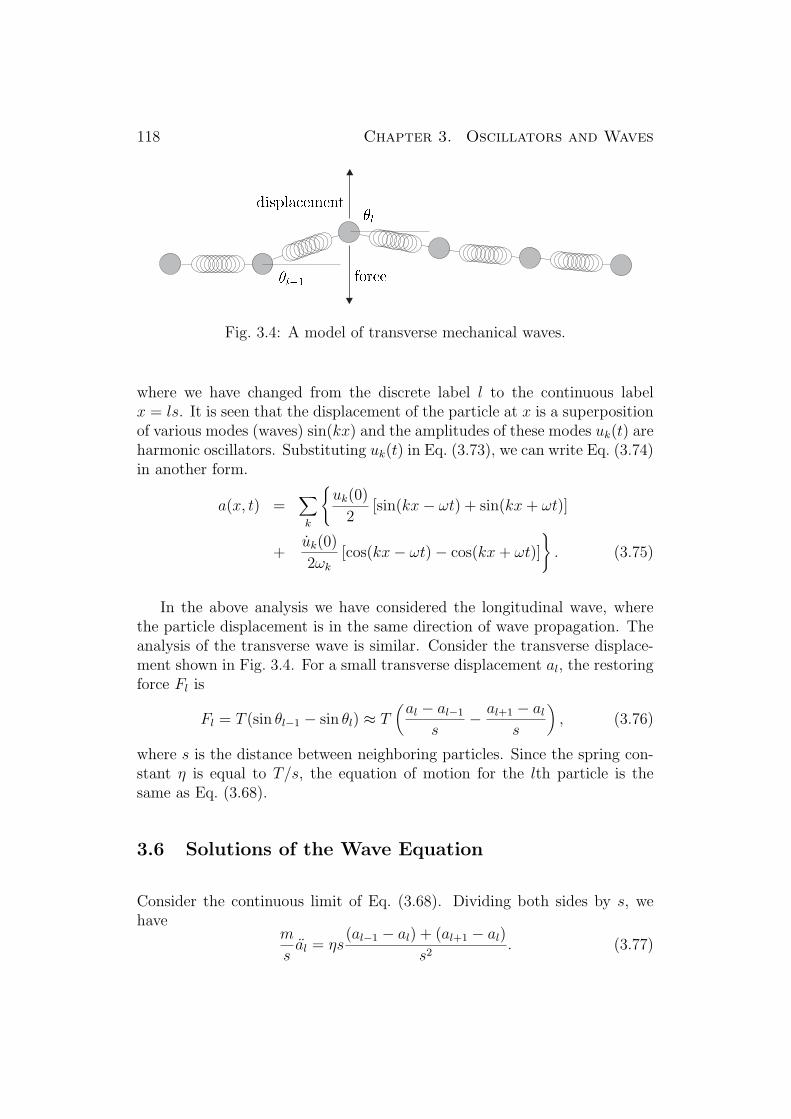
118 Chapter 3. Oscillators and Waves
Fig. 3.4: A model of transverse mechanical waves.
where we have changed from the discrete label l to the continuous labelx = ls. It is seen that the displacement of the particle at x is a superpositionof various modes (waves) sin(kx) and the amplitudes of these modes uk(t) areharmonic oscillators. Substituting uk(t) in Eq. (3.73), we can write Eq. (3.74)in another form.
a(x, t) =∑
k
uk(0)
2[sin(kx− ωt) + sin(kx + ωt)]
+uk(0)
2ωk
[cos(kx− ωt)− cos(kx + ωt)]
. (3.75)
In the above analysis we have considered the longitudinal wave, wherethe particle displacement is in the same direction of wave propagation. Theanalysis of the transverse wave is similar. Consider the transverse displace-ment shown in Fig. 3.4. For a small transverse displacement al, the restoringforce Fl is
Fl = T (sin θl−1 − sin θl) ≈ T(
al − al−1
s− al+1 − al
s
), (3.76)
where s is the distance between neighboring particles. Since the spring con-stant η is equal to T/s, the equation of motion for the lth particle is thesame as Eq. (3.68).
3.6 Solutions of the Wave Equation
Consider the continuous limit of Eq. (3.68). Dividing both sides by s, wehave
m
sal = ηs
(al−1 − al) + (al+1 − al)
s2. (3.77)
3.6. Solutions of the Wave Equation 119
In the limit s → 0, we change from the discrete label l to the continuouslabel x = ls. Eq. (3.77) becomes
ρ∂2a
∂t2= T
∂2a
∂x2, (3.78)
where ρ = m/s is the mass density of the string and T = ηs is the tensionof the string. Eq. (3.78) is a special case of the wave equation called thenondispersive wave equation, which can be written as
∂2a
∂x2− 1
v2
∂2a
∂t2= 0, (3.79)
where v =√
T/ρ is the phase velocity of the wave. To find the solution of
Eq. (3.79), we note that it can be written as
(∂
∂x− 1
v
∂
∂t
) (∂
∂x+
1
v
∂
∂t
)a = 0, (3.80)
or (∂
∂x+
1
v
∂
∂t
) (∂
∂x− 1
v
∂
∂t
)a = 0. (3.81)
Changing variables by
u = x + vt,
w = x− vt, (3.82)
we have∂
∂u
∂
∂wa = 0, (3.83)
or∂
∂w
∂
∂ua = 0. (3.84)
Therefore the general solution is
a(x, t) = f(x− vt) + g(x + vt) (3.85)
for any functions f and g. The actual f and g are determined by the initialconditions a(x, 0) and b(x, 0) ≡ ∂a(x, t)/∂t|t=0. Namely
a(x, 0) = f(x) + g(x),
b(x, 0) = −vf ′(x) + vg′(x). (3.86)

120 Chapter 3. Oscillators and Waves
Differentiating the first equation, we have
a′(x, 0) = f ′(x) + g′(x),
b(x, 0) = −vf ′(x) + vg′(x). (3.87)
From these two equations we can solve f ′(x) and g′(x) in terms of the knownfunctions a′(x, 0) and b(x, 0), and then by integration we have f(x) and g(x)up to the constants of integration.
Alternatively, we may use a technique called separation of variables tosolve Eq. (3.79). Let us assume the solution has the form
a(x, t) = f(x)g(t). (3.88)
Substituting into Eq. (3.79), and dividing by f(x)g(t), we have
f ′′(x)
f(x)=
1
v2
g′′(t)g(t)
. (3.89)
Since the left hand side is a function of x and the right-hand side is a functionof t, they must equal to the same constant independent of x and t. Let usdenote the constant −k2 Then we have
f(x) = e±ikx
g(t) = e±iωt, (3.90)
and ω/k = v.
a(x, t) =∑
k
[c1(k)ei(kx−ωt) + c2(k)ei(kx+ωt)
+ c3(k)e−i(kx−ωt) + c4(k)e−i(kx+ωt)]
=∑
k
[α1(k) sin(kx) sin(ωt) + α2(k) sin(kx) cos(ωt)
+ α3(k) cos(kx) sin(ωt) + α4(k) cos(kx) cos(ωt)] , (3.91)
where ci(k) or αi(k) (i = 1, 2, 3, 4) are constants to be determined by theinitial conditions or the boundary conditions.
If the solution is specified by the initial conditions a(x, 0) and b(x, 0) ≡∂a(x, t)/∂t|t=0, we have
a(x, 0) =∑
k
[α2(k) sin(kx) + α4(k) cos(kx)], (3.92)
b(x, 0) =∑
k
[ωα1(k) sin(kx) + ωα3(k) cos(kx)]. (3.93)

3.7. Energy Density of String Waves 121
These are the Fourier expansion of a(x, 0) and b(x, 0), hence αi(k) (i =1, 2, 3, 4) can be uniquely determined.
If in addition the solution is also specified at the boundary points, forinstance a(0, t) = a(L, t) = 0, which represents a string tied down at x = 0and x = L, we have
a(x, t) =∑
k
[α1(k) sin(kx) sin(ωt) + α2(k) sin(kx) cos(ωt)], (3.94)
where the boundary condition at x = L requires that k = nπ/L. Again theinitial condition a(x, 0) will determine α2(k) and b(x, 0) will determine α1(k).
3.7 Energy Density of String Waves
The time-averaged energy of the string wave is
E =∑
l
ma2l
2+
η(al+1 − al)2
2. (3.95)
In the continuum limit,
E =∫
ρ
2
(∂a
∂t
)2
+T
2
(∂a
∂x
)2 dx. (3.96)
For standing waves, substituting
a(x, t) =∑
k
uk cos(ωt + φ) sin(kx) (3.97)
into Eq. (3.96), we have
E = L∑
k
(ρ
8ω2u2
k +T
8k2u2
k
)=
LT
4
∑
k
k2u2k. (3.98)
For a particular mode represented by k, the energy stored in the mode is
Ek =LT
4k2u2
k. (3.99)
For traveling waves, substituting
a(x, t) =∑
k
uk√2
cos(kx− ωt− φ) (3.100)

122 Chapter 3. Oscillators and Waves
into Eq. (3.96), we have
E = L∑
k
(ρ
4ω2u2
k +T
4k2u2
k
)=
LT
2
∑
k
k2u2k. (3.101)
For a particular mode represented by k, the energy stored in the mode is
Ek =LT
2k2u2
k. (3.102)
3.8 Wave Propagation through an Interface
Imagine a composite string made of two different strings by joining them atx = 0. Let us consider the propagation of string waves through the interfacebetween the two strings when a tension T is applied to the composite string.As the wave goes though the interface, part of the wave will be transmittedand part will be reflected. As we shall see, this is required by the boundaryconditions at the interface. Let the incident wave be
ai(x, t) = αi exp i(kix− ωt), (3.103)
and the transmitted wave be
at(x, t) = αt exp i(ktx− ωt). (3.104)
At x = 0 the mass element must oscillate synchronously, hence the transmit-ted wave must have the same frequency as the incident wave. Yet ki 6= kt
because the two waves have different phase velocities. The amplitudes mustbe continuous across the interface, that is
ai(0, t) = at(0, t), (3.105)
otherwise the position of the interface is undefined. The forces acted on themass elements at both sides of the interface must also be continuous, other-wise the interface will experience an infinite acceleration. As the separations between the mass elements approaches zero, the force on the x < 0 side is
η∆ai =T
s∆ai → T
∂ai
∂x, (3.106)
and force on the x > 0 side is
η∆at =T
s∆at → T
∂at
∂x. (3.107)

3.8. Wave Propagation through an Interface 123
Therefore we have
∂ai
∂x=
∂at
∂x. (3.108)
These boundary conditions lead to
αi = αt,
kiαi = ktαt. (3.109)
Obviously there is a contradiction because ki 6= kt. The contradiction isremoved if there is a reflected wave
ar(x, t) = αr exp i(−kix− ωt). (3.110)
With the addition of a reflected wave, we have
αi + αr = αt,
kiαi − kiαr = ktαt. (3.111)
The solution is
αt =2ki
kt + ki
αi,
αr =ki − kt
kt + ki
αi. (3.112)
If the wave incidences from a medium of larger phase velocity to a mediumof smaller phase velocity, we have ki < kt. In this case the reflected wave isπ out of phase with the incident wave. In the opposite case the the reflectedwave is in phase with the incident wave. The transmitted wave is always inphase with the incident wave.
We have shown in Eq. (3.102) that the energy density of a string wave is
E
L=
T
2k2u2
k. (3.113)
Therefore the energy-density flux flowing toward the interface is
T
2vik
2i α
2i =
Tω
2kiα
2i ,
and that flowing out of the interface is
Tω
2(ktα
2t + kiα
2r).
Substituting αt and αr in Eq. (3.112), we see the incoming energy-density fluxis the same as the outgoing flux, as expected from the energy conservationlaw.

124 Chapter 3. Oscillators and Waves
Fig. 3.5: Oscillating marble in a bowl.
3.9 Exercises
Exercise 3.1. A round marble of mass m and radius r is placed at thebottom of a round bowl of radius R. The marble can roll in the bowl withoutslipping. If the marble is placed slightly off the center of the bowl, as shownin Fig. 3.5. What is its oscillation frequency under the influence of gravity?In this exercise we assume the amplitude of oscillation is so small that therestoring force is proportional to the angle of displacement and the frictionof air is negligible.
Exercise 3.2. The mass of the moon is 7.36 × 10²² kg, its radius is 1.74 ×10⁶ m. Assume the mass distribution is a uniform sphere. We dig a tunnelfrom the moon surface to the other side of the surface through the center ofthe moon, then drop a baseball of 0.2 kg into the tunnel. The initial velocityof the ball is zero. Ignore the gravity from other planets and consider onlythe gravity of the moon. When the baseball reaches the other end, how muchtime has passed? Hint: Use the shell theorem.
Exercise 3.3. Continue with the last exercise. We fill the tunnel with viscousliquid, so that the motion of the baseball is damped. Assume the dampingforce is proportional to its velocity, i.e., fd = −γv. If we wish that thefarthest position the ball can reach is the center of the moon (regardless howlong it will take). What is the minimum value of γ?
Exercise 3.4. On a frictionless table, a weight of mass m is tied to a thinpost at the center of the table by a spring. The spring and the weight canrotate freely around the post without friction. The spring constant is k.

3.9. Exercises 125
Fig. 3.6: A cycloid.
Fig. 3.7: An inverted cycloid.
Show that if the initial displacement is in the x-direction while the initialvelocity is in the y-direction or the initial displacement is in the y-directionwhile the initial velocity is in the x-direction, the trajectory of the weight canbe an ellipse. In these cases, if the total energy of the system is E, and theangular momentum is L, what is the semi-major axis and semi-minor axis ofthe ellipse as functions of E and L? In this exercise we assume the mass ofthe spring is negligible and the length of the spring is zero when unstretched.
Exercise 3.5. If a disk of radius R is rolled horizontally, a point at the edgeof the disk traces out a curve shown in Fig. 3.6. This curve is known as acycloid. (a) What is the equation that describes the curve? (b) Considera bead sliding along an inverted cycloid as shown in Fig. 3.7. The bead isreleased from a height a with zero initial velocity. Show that the time ittakes for the bead to reach the bottom is independent of a.
Exercise 3.6. A small ball of mass m is connected to two identical un-stretched springs as shown in Fig. 3.8. The springs have a length l when

126 Chapter 3. Oscillators and Waves
Fig. 3.8: A soft oscillator.
they are not stretched or compressed. The spring constant is k. If the ball isdisplaced in the direction perpendicular to the springs by a distance d ¿ land released with zero initial velocity, the oscillation period is T . If thedisplacement is 2d, what will be the oscillation period?
Exercise 3.7. A coupled oscillator is shown in Fig. 3.9, in which k1 = k3 = 1,k2 = 3, m1 = 1, and m2 = 2. Show that the motion of both weights canbe described by linear combinations of two oscillatory motions known as thenormal modes. What are the frequencies of the two normal modes? (Note:You do not need to solve the equation of motion to know the frequencies. Ifthe displacement of the two weights are x1(t) and x2(t), You may simplifythe equation of motion by changing variables to y1(t) and y2(t) according to
y1 = a11x1 + a12x2,
y2 = a21x1 + a22x2, (3.114)
where aij are coefficients of linear combinations. If you choose these coeffi-cients wisely, y1(t) and y2(t) will be solutions of independent simple harmonicoscillators.
Exercise 3.8. A 2-gram guitar string is stretched to hold a tension of100 newtons. The distance between the two bridges that fixes the two endsof the string is 80 cm. What is the fundamental oscillation frequency f ofthe string? If the string is pulled up at the center by 1 cm and suddenlyreleased, as shown in Fig. 3.10, what is the amplitude ratio among the wavesof frequencies f , 2f , and 3f?

3.9. Exercises 127
Fig. 3.9: Coupled oscillators.
Fig. 3.10: A guitar string pulled up at the center.
Exercise 3.9. A mechanical toy telephone can be made by connecting thebottoms of two plastic cups with a stretched elastic string. As a personspeaks toward one cup, the sound wave is converted to the vibration of thecup, and the vibration is transmitted by the string to the other cup in whichit is converted back to sound. The string has a linear mass density of 5 g/mwhen it is not stretched. When stretched, its fractional increase of length is0.1% per newton. How much tension must be applied to the string in orderto make the transmission faster than talking through the air directly? Thespeed of sound in the air is 346 m/s. For simplicity in this exercise we ignorethe effect of gravity on the string.
Exercise 3.10. A string is stretched under a tension of 100 newtons. Thelinear mass density ρ of the string is a function of x.
ρ(x) =
1 g/m x < 0,4 g/m 0 ≤ x ≤ L,1 g/m x > L,
where L is 1 m. A wave incidents from the region of x < 0 and transmits tothe region of x > L. The amplitude of the transmitted wave depends on thefrequency of the wave. If the amplitude of the incident wave in the regionof x < 0 is Ai and the amplitude of the transmitted wave in the region ofx > L is At, the transmittance T is defined by
T =A2
t
A2i
.

128 Chapter 3. Oscillators and Waves
Fig. 3.11: Two coupled springs.
Find the frequency of the wave such that the transmittance is 1, i.e., no waveis reflected.
Exercise 3.11. Two equal masses are connected with two identical masslesssprings of spring constant k, as shown in Fig. 3.11. Considering motion in thevertical direction only, what are the angular frequencies of the two normalmodes? Find the ratio of amplitudes of the two masses in each of the twomodes.
Exercise 3.12. It is well known that the oscillation period of a simple har-monic oscillator is independent of its oscillation amplitude. This is becausethe restoring force of a simple harmonic oscillator is always proportional tothe length of stretching, no matter how long it is stretched. However, in thereal world a spring can break when it is stretched too much, therefore a morerealistic spring may be represented by the following potential function:
V (x) = a(e−2αx − 2e−αx),
where a and α are positive constants. The minimum of V (x) is at x = 0,hence the position of the mass can oscillate around x = 0. When x →∞, V (x) → 0, which means there is no restoring force when the spring isstretched too much. In other words, it is broken. Calculate the oscillationperiod of this oscillator as a function of the total energy E, a, and α.

Chapter 4
Statistical and Thermal Physics
4.1 Thermodynamic Variables and Processes
Thermodynamics is the physics about the change of state for macroscopicsystems as a result of energy transfer. A macroscopic system may consistof many particles, and these particles can be atoms and molecules, or evenstars in a galaxy. Because it is impractical to describe the motion of so manyparticles individually, we are concerned only with the state of the macro-scopic system as a whole. The state of a macroscopic system is described bythermodynamic variables such as the pressure P , the volume V , the inter-nal energy U , the temperature T etc. These variables are well defined onlywhen the macroscopic system is in an equilibrium state. For instance, if wedivide a bottle in vacuum into two cells and put gas into one of them, aftera while the gas will reach a state of equilibrium in which we can measure itstemperature, pressure, volume, etc. If we suddenly remove the dividing wallbetween the two cells, the gas will rush into the other cell. After a while anew equilibrium is reached and we have a new pressure, temperature, andvolume. In this process we know the initial state and the final state of thegas, but not the states in between. It is not possible to describe the state ofthe gas between the initial state and the final state because before reachingthe equilibrium the pressure and temperature of the gas are likely to be dif-ferent at each different position. In this case we call the process irreversible.The word “irreversible” does not mean we cannot go back from the finalstate to the initial state. It only means we cannot follow the path from theinitial state to the final state reversely, because we do not know the path
129
130 Chapter 4. Statistical and Thermal Physics
in the first place. To know the path, every state of the macroscopic systemin between must be well defined. In order to meet this condition, we mustkeep the system in equilibrium all the time. A possible way of doing this isby changing the system very slowly, so that the system has enough time tomaintain equilibrium all the time. Then the path can be well defined.
A macroscopic system can be described by different thermodynamic vari-ables in different ways. Thermodynamic variables are not necessarily inde-pendent of each others. They can be related by some equations of state.For instance, for the ideal gas we have the equation of state PV = NkT ,which relates P and V to T . Therefore any two of the three variables P ,V , and T are sufficient to specify the state of the ideal gas. The existenceof the equation of state allows us to treat one thermodynamic variable asan implicit function of other thermodynamic variables, hence in analyzinga thermodynamic problem we may use freely the most convenient variables.For instance, if the thermodynamic process is under the condition of con-stant temperature, then choosing temperature to be one of the independentvariables should greatly simplify the analysis.
In physics of few particles, a particle can have kinetic energy and potentialenergy, and the energy can be changed by the work of external forces. In amacroscopic system we must consider an additional form of energy knownas the internal energy. Consider the energy of a bottle of gas. Even thoughthe bottle itself is not moving, the gas molecules in the bottle is still movingfast in all directions and thus have kinetic energy. If there are forces betweenthe molecules, the molecules also have potential energy. The energy of themolecules is called the internal energy. The fast moving molecules also giverise to a gas pressure, which can be used to do work. Because energy isconserved, if the gas does some work to the outside world, it loses some ofits internal energy. But doing work is not the only way for the bottle of gasto lose energy. If we put the bottle into cold water, the internal energy candecrease without doing apparent work. Energy can flow out of the bottle byheat conduction. Taking into consideration of heat conduction, the law ofenergy conservation reads
dQ = dU + dW, (4.1)
where dQ is the infinitesimal amount of heat transferred to the system, dUis the infinitesimal increase of internal energy, and dW is the infinitesimalamount of work done to the outside world. This is known as the first lawof thermodynamics.

4.2. Entropy in Thermodynamics 131
In addition to the energy conservation law, it is found empirically thatheat cannot be transferred from a low-temperature object to a high-temperatureone without importing work from the outside world. This is known as thesecond law of thermodynamics. Imagine how different the world wouldbe if the second law of thermodynamics could be broken. Then one wouldbe able to connect a machine between a chunk of ice and a tank of boilingwater to make the ice colder and the water hotter. The machine would notneed any fuel because no work would be required. The boiling water couldbe utilized to drive a steam engine doing as much work as we desire, andthe ice could be used to cool our rooms and refrigerators. What a wonderfulworld!
Since the work done by the system to the outside world is
∆W =∫ f
iP dV, (4.2)
it depends on the path from the initial state i to the final state f . As shownin Fig. 4.1, the system does more work going through path A than goingthrough path B. Consequently the amount of heat ∆Q absorbed by thesystem also depends on the path from the initial state to the final state. Forthis reason neither W nor Q can be treated as a thermodynamic variable.To be qualified as a thermodynamic variable, the variable must depend onlyon the state of the system, not the path leading to the state. Because heattransfer is the central problem of thermodynamics, the fact that Q is nota thermodynamic variable causes great inconvenience. As we shall see, thisproblem can be solved by introducing a new variable S known as the entropy,which is qualified as a thermodynamic variable.
4.2 Entropy in Thermodynamics
The concept of entropy was first developed from the study of the efficiencyof Carnot engines. The construction of a Carnot engine is shown in Fig. 4.2.The engine takes heat Q1 from a reservoir at temperature T1, converts someof the heat to work W , and dumps the rest of the heat into another reservoirat temperature T2. After a complete cycle the engine returns to its initialstate. Therefore the internal energy U does not change. By the first law ofthermodynamics, we have
∆Q = Q1 −Q2 = ∆U + W = W. (4.3)

132 Chapter 4. Statistical and Thermal Physics
Fig. 4.1: Two paths with the same initial state and final state but exportingdifferent amount of work.
If W > 0, we must have T1 > T2. Otherwise we can use friction to convert thework back into heat at the reservoir of temperature T2. Then the net effectwill be transporting heat from a lower-temperature reservoir to a higher-temperature one. This violates the second law.
The efficiency of a Carnot engine is defined by
η =W
Q1
=Q1 −Q2
Q1
= 1− Q2
Q1
, (4.4)
where W is the work done by the engine and Q1 is the heat absorbed. Fromthe second law of thermodynamics, η must be smaller than 1, otherwise wecan use the engine to absorb heat Q1 from a reservoir and convert all theheat to work. By friction, the work can be converted back to heat at anotherreservoir which has a higher temperature. Then again the net effect will betransporting heat from a lower-temperature reservoir to a higher-temperatureone, which violates the second law.
A reversible Carnot engine is one that can either absorb heat Q1 at T1,release heat Q2 at T2, while exporting work W , or reversely absorb heat Q2
at T2, release heat Q1 at T1, while importing work W . If we connect twoidentical reversible Carnot engines together and let one export work to drivethe other in the reverse direction, the net effect will be nothing happens.However, because friction in the engines will convert some work into heat,

4.2. Entropy in Thermodynamics 133
Fig. 4.2: A model of thermal engines.
if we use one Carnot engine to drive another in the reverse direction, it isunavoidable that some heat flows from T1 to T2. This makes the enginesirreversible. Therefore in reality there is no reversible engine. Theoreticallywe can imagine an engine with almost no friction. Such an engine is almostreversible.
Let us combine an irreversible Carnot engine and a reversible Carnotengine, and investigate the efficiency of the combined engine. Let engineA be the irreversible engine and B be the reversible engine running in thereverse direction. All the work produced by engine A will be used to driveengine B reversely, as shown in Fig. 4.3. The heat absorbed by the combinedengine at T1 is QA1 − QB1, and the heat released by the combined engineat T2 is QA2 − QB2, while the net production of work is 0. The first law ofthermal dynamics requires that QA2 − QB2 = QA1 − QB1. Let us assumeT1 > T2. Because heat can only flow from the reservoir at temperature T1 tothe reservoir at temperature T2, we have QA1 ≥ QB1, which means
ηB =W
QB1
≥ W
QA1
= ηA. (4.5)
In other words, the efficiency of a reversible Carnot engine is higher thanthat of any irreversible Carnot engine. If engine A is also reversible, we canreverse the roles of the two engines to obtain ηA ≥ ηB. Therefore any tworeversible Carnot engines have the same efficiency.

134 Chapter 4. Statistical and Thermal Physics
Fig. 4.3: A reversible engine driven by an irreversible engine.
Let us use the compression and expansion of the ideal gas to constructan ideal Carnot engine, and see how large the efficiency can be. The cycleof the engine consists of four stages as shown in Fig. 4.4. In the first stagethe gas is kept in thermal contact with a reservoir at T1. The heat absorbedfrom the reservoir makes the gas expand and do positive work. In the secondstage the gas is thermally isolated from the environment while continuingexpanding and doing positive work. In the third stage the gas is kept inthermal contact with a reservoir at T2. The heat released to the reservoirmakes the gas compress and do negative work. In the fourth stage the gas isthermally isolated from the environment while continuing compressing anddoing negative work.
Experimentally it is found that the ideal monoatomic gas has the followingequations of state,
PV = NkT, (4.6)
U =3
2NkT, (4.7)
and as we shall see, these equations of state can be well explained by thekinetic theory of gases. Therefore in the first stage the work done by the gasis
∫ V2
V1
P dV =∫ V2
V1
NkT1
VdV = NkT1 ln
(V2
V1
). (4.8)
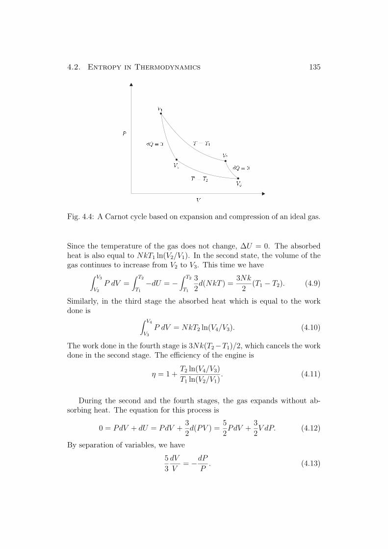
4.2. Entropy in Thermodynamics 135
Fig. 4.4: A Carnot cycle based on expansion and compression of an ideal gas.
Since the temperature of the gas does not change, ∆U = 0. The absorbedheat is also equal to NkT1 ln(V2/V1). In the second state, the volume of thegas continues to increase from V2 to V3. This time we have
∫ V3
V2
P dV =∫ T2
T1
−dU = −∫ T2
T1
3
2d(NkT ) =
3Nk
2(T1 − T2). (4.9)
Similarly, in the third stage the absorbed heat which is equal to the workdone is
∫ V4
V3
P dV = NkT2 ln(V4/V3). (4.10)
The work done in the fourth stage is 3Nk(T2−T1)/2, which cancels the workdone in the second stage. The efficiency of the engine is
η = 1 +T2 ln(V4/V3)
T1 ln(V2/V1). (4.11)
During the second and the fourth stages, the gas expands without ab-sorbing heat. The equation for this process is
0 = PdV + dU = PdV +3
2d(PV ) =
5
2PdV +
3
2V dP. (4.12)
By separation of variables, we have
5
3
dV
V= −dP
P. (4.13)

136 Chapter 4. Statistical and Thermal Physics
After integration, we have
PV53 = c, (4.14)
where c is a constant. This is the equation for the adiabatic expansion of theideal gas. Eq. (4.14) can also be written as
NkTV23 = c. (4.15)
Hence
ln V =3
2ln
(c
NkT
). (4.16)
This gives the relation between V2, V3 and V4, V1.
ln V3 − ln V2 =3
2(ln T1 − ln T2) = −(ln V1 − ln V4). (4.17)
Substituting in Eq. (4.11), we have
η = 1− T2
T1
. (4.18)
Because all the reversible Carnot engines have the same efficiency, this is theuniversal efficiency of reversible Carnot engines. Because
η = 1− Q2
Q1
, (4.19)
Eq. (4.18) can also be written as
Q1
T1
=Q2
T2
. (4.20)
For any Carnot engine we have η = 1−Q2/Q1 ≤ 1− T2/T1, therefore
Q1
T1
≤ Q2
T2
, (4.21)
where the equal sign applies only to reversible Carnot engines.
Let us define a cyclic process to be one that starts from a thermodynamicstate and ends in the same state. Consider a system Γ going through a cyclicprocess that absorbs heat Q from the environment in which the temperatureis not kept constant. Let us construct the process from a sequence of smallcomponent processes, such that each component process absorbs heat Q
(in)i
4.2. Entropy in Thermodynamics 137
or releases heat Q(out)i at temperature Ti. For each component process, let us
use a reversible Carnot engine to supply Q(in)i or absorb Q
(out)i as shown in
Fig. 4.5. Each reversible Carnot engine is constructed in the following way:If the component process absorbs heat, the engine runs between temperatureT1 and Ti, where T1 is the temperature of a reservoir and T1 > Ti. On thecontrary, if the component process releases heat, the engine runs betweentemperature Ti and T2, where T2 is the temperature of another reservoir andTi > T2. Let us separate the two groups of engines and label them by groupG1 and group G2. For the G1 engines, the engine absorbs heat Q
(1)i from a
reservoir kept at T1, and releases heat Q(in)i to the component process at Ti.
From Eq. (4.21) we have
Q(1)i = T1
Q(in)i
Ti
. (4.22)
Therefore the total amount of heat absorbed from the reservoir at T1 is
Q(1) =∑
i∈G1
Q(1)i = T1
∑
i∈G1
Q(in)i
Ti
. (4.23)
Similarly, for the G2 engines the engine absorbs heat Q(out)i from the com-
ponent process at Ti and releases heat Q(2)i to a reservoir kept at T2. From
Eq. (4.21) we have
Q(2)i = T2
Q(out)i
Ti
. (4.24)
Therefore the total amount of heat released to the reservoir at T2 is
Q(2) =∑
i∈G2
Q(2)i = T2
∑
i∈G2
Q(out)i
Ti
. (4.25)
Let us treat Γ and the reversible Carnot engines all together as a compositeengine. The net effect of the composite engine is that it absorbs heat Q(1)
from a reservoir at T1 and releases heat Q(2) to another reservoir at T2. FromEq. (4.21) we have
Q(1)
T1
≤ Q(2)
T2
. (4.26)
We may define a positive ∆Q to be the heat absorbed by a system and anegative ∆Q to be the heat released. Under this notation we have ∆Qi =

138 Chapter 4. Statistical and Thermal Physics
Fig. 4.5: A thermodynamic cycle in which the heat transfer is supplied byCarnot engines.
Q(in)i for i ∈ G1 and ∆Qi = −Q
(out)i for i ∈ G2. Then the net result can be
written as
∑
i
∆Qi
Ti
≤ 0. (4.27)
Let the number of component processes approach infinity. We have
∮ dQ
T≤ 0, (4.28)
where the equal sign holds when the composite engine is reversible. Becauseeach engine of the composite engine is reversible, the equal sign holds whenthe cyclic process of Γ is reversible.
Since
∮ dQ
T= 0 (4.29)
for a reversible cyclic process, we may define a new variable S, which is afunction of the thermodynamic state a, by
S(a) =∫ a
o
dQ
T, (4.30)
4.2. Entropy in Thermodynamics 139
where o is an arbitrary reference state. From Eq. (4.28) we have
∫ a
o
dQ
T+
∫ b
a
dQ
T+
∫ o
b
dQ
T≤ 0 (4.31)
for any integration path connecting o, a, b. Therefore we have
S(b)− S(a) ≥∫ b
a
dQ
T(4.32)
for any two arbitrary states a and b, where the equal sign applies to reversibleprocesses. For an isolated system dQ = 0, we have
S(b) ≥ S(a). (4.33)
This means the entropy of an isolated system can only increase.
We started from the second law of thermodynamics, which states thatheat cannot flow from a place of lower temperature to a place of highertemperature in an isolated system, and arrived at the statement that theentropy of an isolated system can only increase. Conversely, if heat Q couldflow from a place of lower temperature to a place of higher temperature, wewould have
∆S =Q
T1
− Q
T2
< 0. (4.34)
Therefore, that the entropy of an isolated system can only increase is anequivalent statement of the the second law of thermodynamics.
As an example, let us calculate ∆S for an ideal gas when its volumeis changed from Va to Vb while its temperature is changed from Ta to Tb.Substituting U = 3NkT/2 and P/T = Nk/V into
∆S =∫ b
a
dQ
T=
∫ b
a
dU
T+
∫ b
a
PdV
T, (4.35)
we have
∆S =∫ b
a
3Nk
2
dT
T+
∫ b
aNk
dV
V
=3Nk
2(ln Tb − ln Ta) + Nk(ln Vb − ln Va). (4.36)
In other words,
S(T, V ) =3Nk
2ln T + Nk ln V − C, (4.37)

140 Chapter 4. Statistical and Thermal Physics
where C is a constant assigned to be the entropy of the reference state a. Wemay also write S as a function of U and V ,
S(U, V ) =3Nk
2ln U + Nk ln V − C ′, (4.38)
where again C ′ is assigned to be the entropy of the reference state a.
From the definition of S we have
dQ = TdS. (4.39)
This simple relation looks as if Q and S are related by a change of variable.It is not. This is because T is not a function of S only; it depends on otherthermodynamic variable too. As we have seen, S is uniquely defined for eachthermodynamic state up to a constant, whereas it is not possible to assign aunique Q to a thermodynamic state. How much heat a system has absorbeddepends on the history of the system. It is not a conserved quantity becausea system can do work to the outside world. Mathematically we can say 1/Tis an integration factor of dQ. By multiplying dQ with 1/T , we obtain anintegrable differential form dS.
4.3 Thermodynamic Potentials
With dQ = TdS the first law of thermodynamics reads
dU = TdS − PdV. (4.40)
This is a differential form which signifies that U is a function of S and V .Since
dU =
(∂U
∂S
)dS +
(∂U
∂V
)dV, (4.41)
by comparison we have
(∂U
∂S
)
V
= T,
(∂U
∂V
)
S
= −P. (4.42)
4.3. Thermodynamic Potentials 141
For isolated systems, no work is done and no heat is transported to theoutside world, hence dU = 0. If the volume is allowed to change while noheat can flow in or out, we have
dU + PdV = 0. (4.43)
In analogy to the conversion between potential energy φ and work W repre-sented by the equation dφ + dW = 0, we see that U is the potential energyof a system when it is thermally isolated.
For open systems, it is not always convenient to choose S and V as thethermodynamic variables because heat can flow in and out and volume canchange. As a result, dS and dV are not zero. For example, chemical reactionusually occurs under constant P and T . In order to maintain constant T andP , the system must be allowed to exchange heat with the outside world andadjust its volume. In this case it would be more convenient to use P and Tas the thermodynamic variables because they are constants. What will thefirst law become when P and T are used as the thermodynamic variables?Let us consider first the Helmholtz free energy defined as A = U−TS. Fromthis definition we have
dA = dU − TdS − SdT = −dW − SdT = −PdV − SdT. (4.44)
This is a differential form signifying that A is a function of T and V , andtherefore we have
(∂A
∂V
)
T
= −P,
(∂A
∂T
)
V
= −S. (4.45)
For a reversible process that occurs at constant T and V , A does not change.If the volume is allowed to change while temperature is kept constant, wehave
dA + PdV = 0 (4.46)
at constant temperature. In analogy to the conversion between potentialenergy φ and work W represented by the equation dφ+dW = 0, we see thatA is the potential energy of a system when the temperature of the system iskept constant.
Consider an irreversible process pir that brings the system from states1 to state s2 at constant temperature, and the process does an amount of

142 Chapter 4. Statistical and Thermal Physics
work ∆Wir to the outside world which is also kept at the same constanttemperature. The change of Helmholtz free energy is As2 − As1 ≡ ∆Ar
We may bring the system back from s2 to s1 by a reversible process pr
at the same constant temperature. In this process the work ∆Wr done tothe outside world plus the change of Helmholtz free energy is zero, hence∆Wr = −(As1 − As2) = ∆Ar. To ensure that the temperature does notchange, the two processes are carried out under a close contact with a thermalreservoir of temperature T . The work done by the combined process pir + pr
is equal to ∆Wir − (As1 − As2). This work cannot be positive because ifso we are converting heat drawn from a thermal reservoir at temperatureT completely into work. This violates the second law of thermodynamics.Therefore
∆Wir + ∆Ar ≤ 0. (4.47)
As we have mentioned, ∆Wir is the amount of work done to the outsideworld when the state of the system is changed from s1 to s2. Since theoutside world is also kept at a constant temperature T , if we use this amountof work to change the state of the outside world in a reversible way, thechange of Helmholtz free energy for the outside world is
∆Aoutside = −(−∆Wir) = ∆Wir. (4.48)
Note that in this case the work done by the outside world is −∆Wir. Conse-quently, the total change of Helmholtz free energy ∆A is
∆A = ∆Aoutside + ∆Ar ≤ 0. (4.49)
In other words, when a system undergoes an internal irreversible process ata constant temperature T , we have ∆A < 0. In comparison, when a systemundergoes an internal irreversible process at a constant internal energy U ,we have ∆S > 0. If a system is not initially in equilibrium, it can movetoward equilibrium through irreversible processes. If the irreversible processis carried out under the constraint ∆U = 0, we see that the entropy change∆S is positive until the system reaches equilibrium. Therefore we say atequilibrium the entropy S reaches maximum. Similarly, if the irreversibleprocess is carried out under the constraint ∆T = 0, we have ∆A < 0 until thesystem reaches equilibrium. Therefore we say at equilibrium the Helmholtzfree energy A reaches minimum.
We can move a step further to define the Gibbs free energy as G =U − TS + PV . From this definition we have
dG = dU − TdS − SdT + PdV + V dP

4.3. Thermodynamic Potentials 143
= −dW + PdV − SdT + V dP
= −SdT + V dP. (4.50)
This is a differential form signifying that G is a function of T and P , andtherefore we have
(∂G
∂T
)
P
= −S,
(∂G
∂P
)
T
= V. (4.51)
For a reversible process that occurs at constant T and P , G does not change.For an irreversible process, from Eqs. (4.46) and (4.49) we have
∆Aoutside ≤ −∆Ar. (4.52)
For constant P , ∆(PV ) = P∆V , hence ∆G = ∆A + P∆V . Consequently
∆Aoutside + P∆Voutside ≤ −∆Ar − P∆Vsystem, (4.53)
where ∆Voutside is the change of volume of the outside world, ∆Vsystem is thechange of volume of the system, and ∆Voutside = −∆Vsystem. This means thetotal change of the Gibbs free energy ∆G satisfies ∆G ≤ 0. Therefore we sayat equilibrium the Gibbs free energy G reaches minimum when temperatureand pressure are both kept constant.
Another useful thermodynamic variable is the enthalpy defined by H =U + PV . From this definition we have
dH = dU + PdV + V dP = TdS + V dP. (4.54)
This is a differential form signifying that H is a function of S and P , andtherefore we have
(∂H
∂S
)
P
= T,
(∂H
∂P
)
S
= V. (4.55)
At constant pressure dH = TdS = dQ, hence H is commonly used to specifythe heat absorbed in chemical reactions under constant pressure.

144 Chapter 4. Statistical and Thermal Physics
4.4 Kinetic Theory of Ideal Gas
Daniel Bernoulli was the person who first gave a correct analysis of theproperties of gases in terms of the motion of their constituent molecules.At that time (1738), the concept of atoms and molecules was far from beingmature, and there had been no experimental evidence of their existence. Thetheory is completely a result of Bernoulli’s creative thinking.
Consider the statistical distribution of gas particles in a closed rectangularbox. The number of particles with velocity around v is
dN
N= f(v)d3v, (4.56)
where f(v) is the distribution function that satisfies
∫f(v)d3v = 1. (4.57)
Assume the length of the box is L and the area of the wall in the x-directionis A. Within a time interval ∆t, the impulse produced by this group ofparticles bouncing against the wall in the x-direction is
dFx∆t = 2mvxdN, (4.58)
where ∆t = L/vx. The total force on the wall produced by all particles withall velocities is
Fx =2mN
L
∫
vx>0v2
xf(v)d3v. (4.59)
Since by symmetry f(v) = f(−v), Eq. (4.59) can be written as
Fx =mN
L
∫
all vx
v2xf(v)d3v
=mN
Lv2
x, (4.60)
where v2x denotes the average of v2
x. Since v2 = v2x +v2
y +v2z and v2
x = v2y = v2
z ,Eq. (4.60) can be written as
Fx =mN
3Lv2. (4.61)

4.4. Kinetic Theory of Ideal Gas 145
Dividing both sides by A and noting that AL = V is the volume of the gas,we have
PV =2N
3E, (4.62)
where E is the average kinetic energy of the gas particles. Comparing withthe empirical law of ideal gas
PV = NkT, (4.63)
we have
E =3kT
2. (4.64)
Eq. (4.64) establishes a connection between heat and the internal motionof matter. This concept was well ahead of its time, as we note that thetransformation of mechanical energy to heat by friction had not becomeclear until a century later.
Let us consider the form of f(v). By symmetry f(v) cannot depend onthe direction of v, therefore f(v) = f(v2) = f(v2
x + v2y + v2
z). Since vx, vy,and vz are independent random variables, we may decompose the distributionfunction f(v2) into g(v2
x)g(v2y)g(v2
z). By symmetry, the distribution functionsof v2
x, v2y, and v2
z are all the same function g. Let vy = vz = 0, we havef = cg, where c is a constant.
cg(v2x + v2
y + v2z) = g(v2
x)g(v2y)g(v2
z). (4.65)
If a function F satisfies F (x + y) = cF (x)F (y), we may take the derivativeof both sides with respect to x, then let x = 0. This leads to F ′(y) =cF ′(0)F (y). Integrating it with respect to y, we have F (y) = aeby, where aand b are constants. With this observation in mind, we see f(v2) = aebv2
,where a and b are constants to be determined by the following equations:
∫f(v2)d3v = 1. (4.66)
∫v2f(v2)d3v =
3kT
m. (4.67)
Before computing the two integrals in Eqs. (4.66) and (4.67), let us firstevaluate
I0 =∫ ∞
−∞e−x2
dx. (4.68)

146 Chapter 4. Statistical and Thermal Physics
We may write
I20 =
∫ ∞
−∞e−(x2+y2) dxdy =
∫ ∞
0
∫ 2π
0e−r2
r dφdr = π. (4.69)
Hence I0 =√
π. Then we evaluate
I2 =∫
x2e−x2
dx (4.70)
using integration by parts. Let u = x, dv = xe−x2dx.
∫x2e−x2
dx =∫ e−x2
2dx =
√π
2. (4.71)
From the value of I0 and I2, we have
g(vx) =
√m
2πkTexp
(−mv2
x
2kT
), (4.72)
and
∫f(v)d3v =
∫ (m
2πkT
) 32
exp
(−mv2
2kT
)d3v
=∫ (
m
2πkT
) 32
exp
(−mv2
2kT
)4πv2dv. (4.73)
This distribution was first derived by James Clerk Maxwell, and now is knownas the Maxwell distribution. We may express the Maxwell distribution in
terms of energy. Then we have v =√
2E/m and
f(E) dE =2√π
(1
kT
) 32 √
E exp(− E
kT
)dE. (4.74)
Note that f(E) is independent of the mass of the gas particles.
In the discussion above, we have assumed the gas particle distribution isuniform in space. This is true when the gas is not under the influence of anexternal force. If the gas is pushed by an external force, the particle movesalong the direction of the force. As a result, the pressure builds up againstthe force until the balance is reached. Because the pressure is proportionalto density, there will be a density gradient in the direction of the externalforce. In that case, we may no longer assume the density is independent ofposition. The law of ideal gas now reads
P (r) = ρ(r)kT. (4.75)

4.5. Diffusion 147
Consider a thin layer of gas pushed by a conservative force −∇φ(r). Let usassume the normal vector of the layer is in the same direction as the force.The thickness of the layer is dx and the area is A. At equilibrium we have
−N∇φ(r) = ∇P (r)Adx = ∇ρ(r)kTAdx, (4.76)
where N is the total number of gas particles in the layer. Noting thatN/(Adx) = ρ(r), we have
∇ρ(r)
ρ(r)=−∇φ(x)
kT. (4.77)
Therefore
ρ(r) = ρ0 exp
[−φ(r)
kT
]. (4.78)
Combining with Eq. (4.73), we have the phase-space distribution function
F (r,v) = ρ0
(m
2πkT
) 32
exp
−
mv2
2− φ(r)
kT
. (4.79)
4.5 Diffusion
In the center of a large room if a droplet of perfume is released, it takes along while for people at the corner of the room to notice. The farther oneis away from the source of the perfume, the later one detects the fragrance.Although the average speed of gas molecule can be as large as several hundredmeters per second, the fragrant molecules cannot go straight to the someone’snose. In the process of reaching the nose, the molecules suffer from manyrandom collisions with other gas particles. Each collision randomly changesthe direction of moving. Therefore the migration of the molecules is like arandom walk, which takes much longer time to go far than straight movementdoes. As a matter of fact, the transport of fragrant molecules in the realworld is mainly by convective air current. If there exists no air current, itwould take several hours for a significant fraction of the fragrant moleculesto wander a distance of just one meter.
Consider two neighboring regions defined by two slabs. Slab A is atposition x + ∆x and slab B at position x. Because gas particles in thesetwo slabs move in random directions, the chance for a particle to move from

148 Chapter 4. Statistical and Thermal Physics
slab A to slab B is equal to the chance for a particle to move from slab Bto slab A. However, if the total number of particles in slab A is differentfrom that in slab B, the net flux from A to B is not zero. The flux fromA to B is proportional to NATA→B, while from B to A is proportional toNBTB→A, where NA and NB are the number of particles in slab A and slabB respectively, and TA→B=TB→A is the transition probability. The net fluxfrom A to B is simply proportional to NA −NB. In a general mathematicalexpression one can write
J(r, t) = −D∇ρ(r, t), (4.80)
where J(r, t) is the flux vector, and ρ(r, t) is the density distribution. Theproportional constant D is called the diffusion constant.
In the migration process, the number of gas particles in any volume el-ement is conserved. Consider a box at r0 with sides equal to ∆x, ∆y, and∆z. Within a time ∆t, the number of particles flowing into the cell in thex-direction is equal to Jx(r0, t)∆y∆z∆t, and the number of particles flowingout of the cell in the x-direction is equal to Jx(r0 + ∆x, t)∆y∆z∆t. The netaccumulation of particles is
∆n = Jx(r0, t)∆y∆z∆t− Jx(r0 + ∆x, t)∆y∆z∆t. (4.81)
Dividing both sides by ∆V ≡ ∆x∆y∆z and ∆t, in the infinitesimal limit wehave
∂ρ
∂t= −∂Jx
∂x. (4.82)
Taking into account the flows in the y- and z-directions, we have
∂ρ
∂t= −
(∂Jx
∂x+
∂Jy
∂y+
∂Jz
∂z
). (4.83)
Namely,
∇ · J(r, t) +∂ρ(r, t)
∂t= 0. (4.84)
This is known as the continuity equation. Combining Eqs. (4.80) and(4.84), we have
−D∇2ρ(r, t) +∂ρ(r, t)
∂t= 0. (4.85)

4.5. Diffusion 149
This is known as the diffusion equation.
Given an initial density distribution ρ(r, 0), what is the density distribu-tion ρ(r, t)? The problem can be solved by Fourier analysis. Let
ρ(r, t) =
(1√2π
)3 ∫ρ(k, t) exp(ik · r)d3k. (4.86)
Substituting it into the diffusion equation, we have
Dk2ρ(k, t) = −∂ρ(k, t)
∂t. (4.87)
Henceρ(k, t) = ρ(k, 0)e−Dk2t. (4.88)
Because ρ(k, 0) can be obtained from the initial condition ρ(r, 0), ρ(k, t) issolved. Namely
ρ(k, t) =
(1√2π
)3 ∫ρ(r, 0) exp(−ik · r)d3r · e−Dk2t. (4.89)
Let us assume the initial distribution of the fragrant gas is
ρ(r, 0) =ρ0
(2π)32 σ3
exp
(− r2
2σ2
). (4.90)
Then
ρ(k, 0) =ρ0
(2π)32 σ3
(1√2π
)3 ∫exp
(− r2
2σ2
)exp(−ik · r)d3r
=ρ0
(2π)32
exp
(−k2σ2
2
). (4.91)
ρ(k, t) =ρ0
(2π)32
exp
[−k2
(σ2
2+ Dt
)]. (4.92)
ρ(r, t) =
(1√2π
)3 ∫ ρ0
(2π)32
exp
[−k2
(σ2
2+ Dt
)]exp(ik · r)d3k
=ρ0
(2π)32 (σ2 + 2Dt)
32
exp
(− r2
2σ2 + 4Dt
). (4.93)
We see that the fragrant gas expands from its initial radius σ (defined by thestandard deviation of the Gaussian distribution) to
√σ2 + 2Dt after time t.

150 Chapter 4. Statistical and Thermal Physics
4.6 Random Walk
Consider a drunken man walking in a large empty field. For each step i,it takes time ti to complete the walk. The position changes by ri, and thedirection is randomly chosen. After n steps the distance Rn from the originis
R2n =
∣∣∣∣∣n∑
i=1
ri
∣∣∣∣∣2
=n∑
i=1
|ri|2 +∑
i 6=j
2ri · rj. (4.94)
The expectation value of R2n is
E(R2
n
)= nE
(|r|2
)= nr2, (4.95)
because∑
i 6=j 2ri · rj averages to zero. The time it takes to walk so far ist =
∑ni ti, and its expectation value is nE(t) = nt. Let us model the gas
diffusion process by random walk. We call√
r2 the mean-free path lm and tthe mean-free time tm. The mean-square range of diffusion as a function oftime is
R(t)2 = nl2m =tl2mtm
. (4.96)
Since Eq. (4.93) is the density distribution of the gas at time t as a result ofdiffusion, if the probability distribution of the position of a gas molecule att = 0 is
P (r, 0) = δ(r) = limσ→0
1
(2π)32 σ3
exp
(− r2
2σ2
), (4.97)
the probability P (r, t) of finding a gas molecule at time t and at |r| = r isproportional to exp[−r2/(4Dt)]. The mean-square distance from the originis
R(t)2 =
∫∞0 r2 exp
(− r2
4Dt
)4πr2 dr
∫∞0 exp
(− r2
4Dt
)4πr2 dr
= 6Dt. (4.98)
The integrals in the above equation can be evaluated by the formula inEq. (1.247). Hence we have
D =l2m6tm
. (4.99)

4.6. Random Walk 151
It is tantalizing to identify
lmtm
= v, (4.100)
where v is the average velocity
v =∫ ∞
0
(m
2πkT
) 32
v exp
(−mv2
2kT
)4πv2dv
=
√8kT
πm. (4.101)
Note that the evaluation of such integrals can be found in Eq. (1.388). How-ever, because lm is the root-mean-square displacement instead of the meandisplacement, Eq. (4.100) is not exact. Bearing this in mind, we may write
D ≈ lm6
√8kT
πm=
lm3
√2P
πρm
, (4.102)
where P is the pressure and ρm is the mass density of the gas. By measuringthe diffusion constant, one can estimate lm from Eq. (4.102).
Let us use a hard sphere model to describe the gas particle and considerits cross section in collision. Although the physical cross section of a sphereis πa2, where a is the radius of the sphere, the effective cross section incollision is larger. As a matter of fact, two spheres start to touch eachother when their distance is 2a. Therefore the collisional cross section is4πa2 and the average volume a particle occupies is 4πa2tmvr, where vr is theaverage relative velocity between two colliding particles. The mathematicalexpression for vr is
vr =∫|v1 − v2|f(v1)f(v2)d
3v1d3v2, (4.103)
which can be calculated from the Maxwell distribution by changing variables:
vd =1√2
(v1 − v2) ,
vs =1√2
(v1 + v2) . (4.104)
We have
vr =∫|v1 − v2|f(v1)f(v2)d
3v1d3v2 =
√2
∫|vd|f(vs)f(vd)d
3vdd3vs
=√
2 v. (4.105)

152 Chapter 4. Statistical and Thermal Physics
Hence the average volume occupied by a particle is 4√
2πa2tmv ≈ 4√
2πa2lm,and the number density of the gas is ρg ≈ 1/(4
√2πa2lm). We can compare
it with the number density of the same gas particle in the liquid or solidform. Assume in the liquid or solid form the number density ρc is close tothat of the ideal close-packing of spheres, namely ρc =
√2/(8a3). Let Vg be
the volume per mole for the gas (≈ 22.4 l), and Vc be the volume per molefor the liquid or solid form. These two numbers are not difficult to measure.We can obtain a by
ρg
ρc
=Vc
Vg
≈ a
πlm. (4.106)
The number of particles per mole, the Avogadro’s number NA, is then
NA ≈ Vg
4√
2πa2lm. (4.107)
4.7 Boltzmann Distribution
In a typical macroscopic system, the number of equations that govern themotion of the constituent atoms or molecules can be as large as 1023. Theseequations are coupled to each others as a result of interaction between de-grees of freedom. Even if such a large number of equations can be solved bysome supercomputer in the future, there will be too much information, usefulor not, in the solutions to be digested by a human being. In most cases, weare not so concerned with the individual dynamics of each degree of freedom.Instead, we are concerned with the average dynamics of the system. The keypoint is that each macroscopic state of matter corresponds to an extremelylarge number of microscopic states. Some macroscopic states are more prob-able than others because they correspond to a larger number of microscopicstates. In order to find an economic way to connect macroscopic states withmicroscopic states, Boltzmann postulated that for an interactive system atequilibrium, the system has an equal probability in every microscopic state.This revolutionary idea led to a powerful method—statistical mechanics.
Let us denote pi the probability of the ith microscopic state and Tij thetransition probability from state j to i. Since the equations of motion for themicroscopic degrees of freedom are time-reversible, we may assume Tij = Tji.The rate of change of pi can be written as
dpi
dt=
∑
j
Tijpj −∑
j
Tjipi =∑
j
Tij(pj − pi). (4.108)

4.7. Boltzmann Distribution 153
Let us define a quantity s by
s ≡ −∑
i
pi ln pi, (4.109)
then we have
ds
dt= −∑
i
dpi
dt(1 + ln pi). (4.110)
Substituting Eq. (4.108) in, we have
ds
dt= −∑
ij
Tij(pj − pi)(1 + ln pi). (4.111)
Since i, j are dummy indices, we may exchange them to get
ds
dt= −∑
ij
Tij(pi − pj)(1 + ln pj)
= −∑
ij
Tij(pj − pi)(−1− ln pj). (4.112)
Adding these two equations, we have
ds
dt= −1
2
∑
ij
Tij(pj − pi)(ln pi − ln pj). (4.113)
Since the right-hand side of Eq. (4.113) is always positive, we conclude thats always increases with time. Since pi are constrained by the condition∑
i pi = 1, we can find the maximum of s by the method of Lagrange’smultipliers. Namely
∂s
∂pi
+ λ∂
∂pi
∑
j
pj − 1
= − ln pi − 1 + λ = 0, (4.114)
where λ is the Lagrange’s multiplier associated with the constraint∑
i pi = 1.Eq. (4.114) leads to the conclusion that as t → ∞, pi = pj for any i, j.Namely the probability of every microscopic state is the same.
We may look at I ≡ e−s as the amount of information we have at hand. Ifwe know the system is exactly in the mth state, we have the full informationabout the system. In this case pm = 1, pi = 0 for i 6= m, therefore s = 0, I =1. If every state has the same probability then we have the least informationabout the system. In this case pi = 1/N , s = ln N , therefore I = 1/N , where

154 Chapter 4. Statistical and Thermal Physics
N is the total number of microscopic states. Because we cannot keep trackof all the state transitions, as time goes by information is lost. That is, sincreases with time.
Let us consider a macroscopic system made of a large number of micro-scopic parts, each of which is characterized by its microscopic state. Forsimplicity, let us distinguish the microscopic states only by their energy Ei.Assume there are ni microscopic systems, each of energy Ei. One has
∑
i
ni = N, (4.115)
∑
i
niEi = E, (4.116)
where N is the number of microscopic systems and E is the total energy. Foreach set ni there are Γ(ni) ways of constructing the macroscopic system.
Γ(ni) =N !∏i ni!
. (4.117)
We may refer to of each the Γ(ni) ways as a microscopic state of the macro-scopic system. In Eq. (4.114) we have shown that as t →∞ the probabilityof every microscopic state is the same, hence a set nk is less probable thananother set nl if Γ(nk) is smaller than Γ(nl). Consequently the mostprobable distribution of ni is the one that maximizes Γ under the constraintof Eqs. (4.115) and (4.116). By the method of Lagrange multipliers
∂
∂ni
[ln Γ(ni) + α(N −∑
i
ni) + β(E −∑
i
niEi)
]= 0. (4.118)
Using Stirling’s approximation ln N ! ≈ N ln N −N ,
ln Γ(ni) ≈ N ln N −∑
i
ni ln ni. (4.119)
Eq. (4.118) becomes
−(ln ni + 1)− α− βEi = 0, (4.120)
hence ni ∝ exp(−βEi), which means the probability of finding a microscopicsystem with energy Ei is proportional to exp(−βEi).
Now consider two macroscopic systems, the total number of ways of con-structing the two systems is Γ(ni) = Γ1(n1i)Γ2(n2i). If they are iso-lated, the individual distributions are determined by
∂
∂n1i
[ln Γ1(n1i) + α1
(N1 −
∑
i
n1i
)+ β1
(E1 −
∑
i
n1iE1i
)]= 0
(4.121)

4.7. Boltzmann Distribution 155
and
∂
∂n2i
[ln Γ2(n2i) + α2
(N2 −
∑
i
n2i
)+ β2
(E2 −
∑
i
n2iE2i
)]= 0
(4.122)respectively. If the two systems are brought to thermal equilibrium, thereis only one constraint of total energy,
∑i n1iE1i +
∑i n2iE2i = E, instead of
two independent energy constraints∑
i n1iE1i = E1,∑
i n2iE2i = E2. Fewerconstraints mean more possibility. Therefore we have Γeq ≥ Γiso. Equalityoccurs only if β1 = β2 initially. This means when a system approachesequilibrium, ln Γ increases until the β of each of its parts becomes equal.This is a strong indication that ln Γ is related to entropy and β is a measureof temperature.
Let us investigate the relation between ln Γ and the internal energy of thesystem. The internal energy U of the system is U =
∑i niEi, and
dU =∑
i
Eidni +∑
i
nidEi. (4.123)
On the right-hand side the first term is the change of thermal energy becausedni changes the state distribution of the system. In contrast, the secondterm does not change the state distribution, instead it changes uniformly theenergy of all the microscopic systems in the same state i. Such an energychange is produced by adiabatic macroscopic external forces. Therefore thesecond term is the work done by external forces. From
ln Γ = N ln N −∑
i
ni ln ni, (4.124)
and
ni =Ne−βEi
Q, (4.125)
Q =∑
i
e−βEi , (4.126)
we have
d ln Γ = −∑
i
(ln ni + 1)dni
= −∑
i
(ln N − βEi − ln Q + 1)dni. (4.127)
Because ln N − ln Q + 1 is a constant and∑
i dni = dN = 0, we have
d ln Γ =∑
i
βEidni. (4.128)

156 Chapter 4. Statistical and Thermal Physics
In other words,
d ln Γ
β= d
(∑
i
Eini
)−∑
i
nidEi = dU + dW, (4.129)
where dW is the work done by the system to the outside world. Compar-ing with the first law of thermodynamics dU = dQ − dW , and noting thedefinition dQ = TdS, we have
S = k ln Γ, (4.130)
β =1
kT. (4.131)
Eq. (4.130) relates the number of microscopic states Γ to the macroscopicquantity S, and Eq. (4.131) yields
ni ∝ exp(− Ei
kT
), (4.132)
which is known as the Boltzmann distribution.
Using Eq. (4.119), and the fact∑
i ni = N , we have
S
N= −k
∑
i
ni
Nln
(ni
N
). (4.133)
If we interpret ni/N as the probability in the state i, according to Eq. (4.113),S/N always increases with time. We see that statistical mechanics providesa clear way to understand the second law of thermodynamics from a micro-scopic point of view.
By calculating Γ as a function of macroscopic variables, such as the energyE, the volume V etc., one can obtain the entropy function S(E, V ). FromS(E, V ) one can obtain the equation of macroscopic state. This is howstatistical mechanics works. As an example, let us derive the equation ofstate for the ideal gas. Envision N independent particles in a box of volumeV . For each particle the number of possible states is proportional to V .Because the particles move independently, the number of microscopic statesfor the whole system is proportional to V N . In addition, the particles canhave different momenta subjected to the constraint
3N∑
i=1
p2i /(2m) = E. (4.134)

4.7. Boltzmann Distribution 157
Considering the surface area of a 3N -dimensional sphere, the number of
states with total energy E is proportional to√
E3N−1
. Therefore one has
Γ(E, V ) = CV N√
E3N−1
, (4.135)
where C is a proportional constant depending only on N and m and
S(E, V ) = k ln Γ(E, V ) ≈ kN ln V +3
2kN ln E + k ln C(N). (4.136)
From the thermodynamic relation dE = TdS − PdV one has
dS =1
TdE +
P
TdV, (4.137)
hence
P
T=
∂S
∂V= kN/V, (4.138)
1
T=
∂S
∂E= 3kN/(2E). (4.139)
These are the equations of state for the ideal gas.
The entropy function is not always the most convenient to start with.For example, in studying a system which is in thermal contact with a largeheat bath, it is more convenient to describe the system as a function of (T, V )than (E, V ) because T is fixed by the temperature of the bath. Therefore oneuses the Helmholtz free energy A = E − TS, in view of dA = −SdT −PdV .Since the system can exchange energy with the heat bath, its energy is not afixed value as in an isolated system. Instead the energy follows a probabilitydistribution, namely the Boltzmann distribution. The expectation value is
E =
∑Ei
EiΓ(N, V,Ei)e−Ei/kT
∑Ei
Γ(N, V,Ei)e−Ei/kT. (4.140)
Let us define the canonical partition function
Q(N, V, T ) ≡ ∑
Ei
Γ(N, V,Ei)e−Ei/kT , (4.141)
one has
E =−∂ ln Q
∂β. (4.142)
On the other hand,
E = A− T∂A
∂T= −T 2∂(A/T )
∂T=
∂(A/kT )
∂β, (4.143)
therefore A = −kT ln Q. By calculating Q from the microscopic states, oneobtains the macroscopic quantity A.

158 Chapter 4. Statistical and Thermal Physics
4.8 Sedimentation and Brownian Motion
If you have watched a sedimentation pool, you must have found that heavyparticles such as marbles and sands are all dropped to the bottom. But,for small particles the behavior is quite different. Not all of them drop tothe bottom, nevertheless the concentration increases near the bottom. Toobtain clear water, we must drain the pool from near the top, where theconcentration of the particles are smallest. These particles are heavier thanwater, why don’t they all drop to the bottom? The Boltzmann distributionprovides the answer. Let the vertical distance from the bottom be z. Thepotential energy for a particle at z is mgz, where m is the effective mass ofthe particle. The effective mass is ms − mb, where ms is the mass of theparticle and mb is the mass of the water of the same volume. From theBoltzmann distribution we have
ρ(z) = ρ(0) exp(−mgz
kT
), (4.144)
where ρ(z) is the concentration at z. For heavy particles, mgz À kT , theconcentration is negligibly small for z > 0. In other words they all drop tothe bottom. For particles of three times the water density, if the particlediameter is 10 nm, at 300K the height at which the concentration drops to1/e is 5 cm. By measuring the 1/e height of sedimentation, one can obtainthe value of k, and then the Avogadro’s number by NA = R/k, where R isthe gas constant.
The suspended particles are not hanging still in the water. They bouncearound like random walk. This random motion can be observed under mi-croscopes, and it is known as the Brownian motion. If the radius of the sus-pended particles is r and the viscosity of water is η, then according to Stokeslaw the particles fall down under gravity at a drift velocity mg/(6πrη). Thedown drift flux ρ(z)mg/(6πrη) must be balanced by the diffusion caused bythe concentration gradient. We have
Ddρ(z)
dz+
mg
6πrηρ(z) = 0. (4.145)
The solution is
ρ(z) = ρ(0) exp
(− mgz
6πrηD
). (4.146)
Comparing with Eq. (4.144), we have
D =kT
6πrη. (4.147)

4.9. Osmotic Pressure 159
By observing the random motion of a suspended particle under a microscope,one can obtain the mean-free path and mean free time and then the diffusionconstant by Eq. (4.99). From the diffusion constant and Eq. (4.147), one canobtain the value of k, and then the Avogadro’s number again by N = R/k.
4.9 Osmotic Pressure
Consider the particles in a suspension solution. If the particles are under theinfluence of an external conservative force F (r) = −∇φ(r), then accordingto the Boltzmann distribution the concentration follows
ρ(r) = ρ0 exp
[−φ(r)
kT
]. (4.148)
Since the particles’ average velocity is zero, the net force applied to themmust be zero. The external force per unit volume is −ρ(r)∇φ(r). This forcemust be balanced by a pressure difference that arises from the concentrationdifference. This is exactly the pressure difference that drives the diffusion.Let the pressure at r be P (r). For a thin-slab volume element of area Aand thickness dx, if the normal vector of the slab is in the same direction as∇P (r), the force from the pressure difference on the two sides of the slab is−A∇Pdx. Therefore the force from the pressure difference per unit volumeis −∇P (r). The balance condition is
ρ(r)∇φ(r) +∇P (r) = 0. (4.149)
Taking the gradient of Eq. (4.148), we have
∇ρ(r) = −ρ(r)
kT∇φ(r). (4.150)
Comparing Eq. (4.149) and Eq. (4.150), we have
P (r) = ρ(r)kT. (4.151)
This is the extra pressure caused by the diffusion of the suspended particles,and is known as the osmotic pressure.
We may also understand the osmotic pressure from the point of viewof entropy. When suspended particles are mixed into a solvent to form asolution, the suspended particles introduce a large number of microscopicstates. This increases the entropy. If we assume that the concentration of

160 Chapter 4. Statistical and Thermal Physics
the suspended particles is small, so that the particles move independently ofeach other, then
Γs = C(N)V Nf(E), (4.152)
where f(E) represents the total number of velocity combinations the sus-pended particles can have under the constraint that the total energy of themis E. Since the suspended particles form a subsystem that can exchange en-ergy with the large system of the solvent, E is not a fixed number. Instead,the temperature is approximately fixed because the small energy exchangewill not change the solvent temperature significantly. In this situation weshould choose the Helmholtz free energy A(N, T, V ) as the thermal dynam-ics variable to calculate. To obtain A(N, T, V ), we should first evaluate thepartition function Q(N, T, V ).
Q(N, T, V ) =∫
C(N)V Nf(E) exp(− E
kT
)dE. (4.153)
Therefore
A(N, T, V ) = −kT ln Q = −kT ln C(N)− kTN ln V − kTD(T ), (4.154)
where
D(T ) = ln[∫
f(E) exp(− E
kT
)dE
]. (4.155)
From the relation
−P =
(∂A
∂V
)
T
, (4.156)
we have
−P = −kT(
N
V
). (4.157)
In other words,P = kTρ, (4.158)
where ρ is the concentration. This is exactly the same as Eq. (4.151). Notethat we have only considered the pressure produced by the subsystem of thesuspended particles, therefore Eq. (4.158) is the pressure difference betweenthe suspension solution and the pure solvent. The pressure of the pure solventcan be obtained from Γ or Q of the solvent, which is not included in thecalculation of this section.
It is known that plants gather water by the capillary effect. Since inmost cases the leaves are surrounded by less moisture than the roots, wateris transported from the roots to the leaves. However, because the capillary

4.10. Boiling Point 161
effect works in both directions, it does not explain why some plants, suchas coconut and watermelon, are able to gather a large quantity of waterin their fruits. It turns out that a little chemicals dissolved in water willhelp. Dissolving 30 g of fructose or 5 g of NaCl into 1 liter of water, youget a concentration of 0.17 mole of molecules or ions per liter. The osmoticpressure of this solution is about 0.17 × 22.4 = 3.9 atm. Such a pressure islarge enough to raise the solution to 40 meters high. Plants have developedsemipermeable membranes to maintain an osmotic pressure that attractswater. In dry area, plants must maintain a high osmotic pressure to competefor water. If you grow such plants, you should be careful not to water themtoo much. Too much water will cause the cells to burst, and that kills theplant. The osmotic pressure also explains why watermelon grown in dryersandy soil is sweeter.
4.10 Boiling Point
In Taiwan, tea tasting and mountain hiking are two popular recreationalactivities. If you boil water on a high mountain to prepare tea, you maynotice that the boiling point is below 100C. In contrast, if you dissolve somesalt into the water, you may know that the boiling point rises. How do weunderstand these phenomena?
Since the boiling occurs in the open atmosphere, if the cover of the pot isnot tightly sealed, the pressure is equal to the air pressure of the environment,which is held constant. Inside the pot the temperature also remains constantat the boiling point. As we have seen, in this case the best thermodynamicvariable to choose is the Gibbs free energy G.
Because liquid water and water vapor are two different phases, the Gibbsfree energy are two different functions of T and P . We have
dGg = VgdP − SgdT,
dGl = VldP − SldT, (4.159)
where Gg is the free energy of the gas-phase water and Gl is that of theliquid-phase water. Since both V and S are proportional to the number ofmolecules, we may rewrite Eq. (4.159) as
dgg = vgdP − sgdT,
dgl = vldP − sldT, (4.160)

162 Chapter 4. Statistical and Thermal Physics
where gg, vg, and sg are the specific Gibbs free energy (Gibbs free energyper mole), the specific volume (volume per mole), and the specific entropy(entropy per mole) respectively for the gas phase. Similarly, gl, vl, and sl arethe same quantities for the liquid phase.
As we have shown in Section 4.3, at equilibrium the total change of Gmust be zero. Therefore at the boiling point the gain of G for the gas mustbe equal to the loss of G for the liquid if some water molecules are convertedfrom the liquid phase to the gas phase. If m moles of water molecules areconverted, the change of Gg is mgg, and the change of Gl is −mgl. The totalchange of G is zero means gg = gl at the boiling point. Since gg and gl aretwo different functions of T and P , in principle we can use the conditiongg = gl to find T as an implicit function of P . Then for every P we have acorresponding T at which the water boils. In other words, in principle wecan find the boiling temperature T as a function of P from the conditiongg = gl. However, in practice we do not know the form of gg or gl, can westill say something about the change of boiling temperature resulting fromthe change of pressure?
Empirically we know water boils at 1 atm, 100C. We may extrapolatethe implicit function T (P ) near this known point. From
dgg = vgdP − sgdT = dgl = vldP − sldT. (4.161)
we have
dP
dT=
sg − sl
vg − vl
. (4.162)
Since the change of entropy sl − sg is done at constant T , we have ql =T (sg − sl) and
dP
dT=
ql
T (vg − vl), (4.163)
where ql is the molar latent heat that must be supplied to vaporize the liquid.Eq. (4.163) is known as the Clapeyron equation.
Let us use the Clapeyron equation to calculate the boiling point at 2000 mabove the sea level. The average mass of air per mole is 28.8 g. From theBoltzmann distribution, at 2000-m height the air pressure drops by 21%,assuming the temperature is 20C. That is ∆P = −2.1 × 10⁴ Pa. Since thespecific volume of liquid water is much smaller than that of the water vapor,

4.10. Boiling Point 163
we may ignore vl in the Clapeyron equation in comparison with vg. Then wecan integrate the Clapeyron equation to get a relation between ∆P and ∆T ,assuming the equation of state for the water vapor is the same as that of theideal gas. Namely, one has
dP
dT=
qlP
NkT 2. (4.164)
The equation can be integrated by separation of variables. That is
∆(ln P ) = − ql
Nk∆
(1
T
). (4.165)
The molar latent heat for water is 40860 J/mole. We have
ln 0.79 = − 40860
6.02× 1023 × 1.38× 10−23
(1
T− 1
373
), (4.166)
which gives the boiling point T = 93.4C.
We can estimate the boiling point of a solution in a similar way. If wedissolve 5 g of NaCl in to 1 liter of water, we get 0.17 mole of ions in thesolution. According to Raoult’s law, the vapor pressure of the solution Ps
will be reduced relative to the vapor pressure of pure water Pw according tothe following equation.
Ps
Pw
=ρl − ρi
ρl
, (4.167)
where ρl is the number density of water and ρi is the number density of ions.The amount of vapor pressure difference one must compensate by increasingthe temperature is therefore
∆P = Pw − Ps =Pwρi
ρl
. (4.168)
Taking Pw = 1 atm, we have ∆Pv = 0.17× 0.018 atm = 3.09× 10² Pa. Usingthe Clapeyron equation again, we obtain ∆T ≈ 0.087C.
The vapor pressure difference ∆P can also be derived without usingRaoult’s law. Consider the system shown in Fig. 4.6. The vapor is in equilib-rium with both the solution and the pure water at the boiling temperatureof the solution. At this temperature the vapor pressure of the pure waterexceeds the boiling vapor pressure of the solution by
∆P = Poρv
ρl
, (4.169)
where Po is the osmotic pressure and ρv, ρl are the densities of the watervapor and the solution at the boiling point respectively. Using the relationPw = ρvkT and Po = ρikT , we find that Eq. (4.169) is the same as Eq. (4.168).

164 Chapter 4. Statistical and Thermal Physics
Fig. 4.6: Vapor pressures of solutions. The osmotic pressure Po is equal toPA − PB = ρlgh, and the difference in vapor pressure between the solutionand the pure water is PA − PC = −ρvgh, where h is the height differencebetween the solution and the pure water.
4.11 Exercises
Exercise 4.1. The highest point of NTU campus is the Ling-Tou mountain atXi-Tou experimental forest. The height is 2025 m. Assume the temperatureof the atmosphere is fixed at 20C. What is the ratio of oxygen concentrationat this point to that at sea level?
Exercise 4.2. A thermally insulated box is divided into two compartmentsby a thin rigid wall. The volume of compartment A is 2 liters, and the volumeof compartment B is 1 liter. We fill compartment A with 1 mole of He gas at600 K and compartment B with 1 mole of Ne gas at 300 K. Then we drill asmall hole on the wall between the two compartments so that the two gasescan mix slowly with each other. After equilibrium is reached, how much isthe change of entropy? In this exercise we assume both gases are ideal gas.
Exercise 4.3. The equation of state of a thermal dynamic system is PV =NkT . If we treat the internal energy U of the system as a function of volumeV and temperature T , show that U is a function of T only. Namely,
(∂U
∂V
)
T
= 0. (4.170)

4.11. Exercises 165
Hint: Since we are using V and T as the independent variables, it is reason-able to start from the Helmholtz free energy
dA = −SdT − PdV, (4.171)
which yields(
∂A
∂V
)
T
= −P. (4.172)
Since A = U − TS, we have(
∂U
∂V
)
T
− T
(∂S
∂V
)
T
= −P. (4.173)
Because S is not in the equation of state, we had better get rid of it, otherwisewe would not know what to do with it. To do that, you need to derive therelation
(∂S
∂V
)
T
=
(∂P
∂T
)
V
, (4.174)
from dA = −SdT − PdV . Then you can use the equation of state to prove(∂U/∂V )T = 0.
Exercise 4.4. If a 2-kg frozen chicken takes 10 hours to defrost, under thesame condition how long does it take to defrost a 2-ton elephant? Althougha chicken has a different body shape from an elephant, in this problem weassume both were curled up like a meat ball when they were frozen. Wealso assume the heat conductivity, specific heat, and mass density for bothare the same. The time to defrost can be defined by that the temperatureat the center reaches 0.9T0, where T0 is the absolute temperature of theenvironment.
Exercise 4.5. Dry ice can be made by suddenly opening the valve of ahigh-pressure CO2 tank. The temperature of CO2 in the tank is 25C. Theprocess can be approximated by a simple model in which the CO2 gas goesthrough adiabatic expansion from pressure P = P0 to P = 1 atm. The icepoint for CO2 is −78C. What is the minimum value of P0? For simplicity,we assume the heat capacity of CO2 is approximately 7k/2 per molecule atconstant pressure, and 5k/2 per molecule at constant volume, where k is theBoltzmann constant.
Exercise 4.6. A thick round pipe buried under 0C ground is used to trans-port hot water of 90C. The inner radius of the pipe is 2 cm and the outer
166 Chapter 4. Statistical and Thermal Physics
radius is 5 cm. If the inner surface of the pipe is maintained at 90C andthe outer surface at 0C, what is the temperature between the two surfacesas a function of r, where r is the distance from the center of the pipe? Inthis exercise we assume the specific heat of the pipe does not change withtemperature. We also ignore thermal radiation.
Exercise 4.7. A factory extracts pure water from sea water at 300 K byusing semipermeable membrane to filter out ions. The ion concentration ofsea water is approximately 1 mole per liter. The factory extracts 1 liter ofpure water from every 5 liters of sea water. How much minimum work mustbe done for each liter of pure water so produced?
Exercise 4.8. A high-speed centrifugal machine is used to separate U235F6
gas from U238F6 gas to make fuel for nuclear reactors. The machine is madeof a tube 20 meters long lying horizontally on the x-y plane and rotatingaround the z-axis which passes through the mid-point of the tube. The tubeis filled with a natural mixture of U235F6 and U238F6. The speed of rotationis 3000 round per minute. The natural abundance of U235 is 0.72%, and thatof U238 is 99.27%. After the two gases reach equilibrium, what is the ratio ofnumber density between U235F6 and U238F6 at the two far ends of the tube?Assume the temperature of the gases is 300 K. The mass of Fluorine atom is19 g/mole. In this exercise some numerical integrations are needed. If yourhand-held calculator cannot do numerical integration, you may express theanswer in terms of the following function:
F (x) =∫ x
0et2dt.
Namely, assume the value of F (x) is known for all x.
Exercise 4.9. A high-pressure stewpot can greatly reduce the cooking time.One may view cooking as some kind of chemical reaction. From the orderof the activation energy one may estimate that for every 5C increase oftemperature, the reaction rate is doubled. If a sealed high-pressure stewpotcan maintain a pressure of 1.1 atm, by how much one can speed up thecooking? Namely, if the cooking takes 1 hour at 1 atm, how long will ittake at 1.1 atm? In this exercise we assume the maximum temperature thestewpot can reach is the boiling point of water.
Exercise 4.10. In northern Taiwan, most people use electric heaters to keeptheir rooms warm during some cold days. Consider an insulated room sealedwith 1-atm air. No heat or air can leak out of the room. The size of theroom is 10 m× 6 m× 4 m. If the air in the room is an ideal gas with a heat

4.11. Exercises 167
capacity per molecule at constant volume equal to 5k/2, how much energyit takes to heat up the room from 15C to 20C with an electric heater?
The energy-efficiency rating (EER) of an air-conditioner is defined by howmany joules per second are removed for each watt of power it draws. TypicalEER is 2.7 for small air-conditioners. If one uses an air-conditioner in thereverse direction to heat up the room, how much energy is needed to heat upthe room from 15C to 20C? Although physically the EER will vary withboth the indoor temperature and the outdoor temperature, for simplicity weassume the EER is a constant of 2.7.
If one uses an ideal Carnot engine running reversely to pump heat fromoutside into the room, where the temperature outside is also 15C, how muchwork is needed to fulfill the same purpose?
Exercise 4.11. Consider two thermally insulated 100-liter tanks. One isfilled with 100C water and the other with 0C water. If we use the twotanks to drive an ideal Carnot engine, what is the maximum work the enginecan produce? The heat capacity of water is 4.18 J/(K· g) in the temperaturerange considered here.
Exercise 4.12. Consider a spherical water droplet of radius R surroundedby air of water-vapor concentration x in a large room. The air and thedroplet are at the same temperature T . The density of the water dropletis ρw, and the density of the pure water vapor is ρv. The concentration ismeasured by the fraction of water molecules in the air. The water dropletwill slowly evaporate as a result of the diffusion of water molecules. Since atthe surface of the water droplet the liquid-phase water is in equilibrium withthe gas-phase water, it is reasonable to assume that right above the surfaceof the water droplet the water-vapor concentration is x0, which correspondsto the saturated vapor pressure at T , and far away from the droplet thewater concentration is x (x < x0) in the steady state. Then we have asteady-state concentration gradient of water molecules in the radial direction.This concentration gradient will drive the transport of water molecules bydiffusion. The diffusion coefficient is D. What is the rate of change of theradius of the water droplet dR/dt as a function of x, x0, ρw, ρv, R, and D? Inthis exercise we assume the evaporation rate is small so that the temperatureof the droplet remains constant.
Exercise 4.13. The open-circuit voltage V of a battery is a function of

168 Chapter 4. Statistical and Thermal Physics
temperature T .
V = 12 + 0.05(T − T0)− 0.0005(T − T0)2,
where V is measured in volts and T0 = 25C. If the battery is kept at 18Cby thermal contact with a heat reservoir, for each Coulomb of electricity thatflows through the battery, how much heat is absorbed by the battery fromthe reservoir? We assume the battery has no internal resistance.
Exercise 4.14. A gas is modeled as hard spheres undergoing random col-lisions. If the temperature is increased from T to 2T at the same pressure,by what factor the diffusion coefficient will change? If the pressure is in-crease from P to 2P at the same temperature, by what factor the diffusioncoefficient will change?
Exercise 4.15. A person is confined in a sealed room. There is a roundhole on the wall connected to the atmosphere through which oxygen candiffuse into the room. The hole is filled with porous material such that airconvection through the hole is not possible. The thickness of the wall is10 cm. In order for the person to remain comfortable, the concentration ofthe oxygen must not be lower than 80% of its normal concentration at 1 bar(100 kPa). Because a person consumes 30 g of oxygen per hour, the hole mustbe large enough to supply this amount of oxygen. If the oxygen molecule ismodeled as a hard sphere of 0.3-nm diameter, what is the minimum area ofthe hole? In this problem we assume the temperature is 300 K and diffusionis the only mechanism oxygen can pass through the hole. We also note thatoxygen occupies 20.94% of air by volume. To simplify the calculation wetreat nitrogen and carbon dioxide molecules as hard spheres that have thesame diameter and mass as the oxygen molecule, and assume that inside theroom the concentration of oxygen is uniform.
Exercise 4.16. In a three-dimensional world, if gas diffusion is modeled byrandom walk, the diffusion coefficient D is related to the mean free path lmby
D ≈ lm6
√8kT
πm,
where T is the temperature and m is the mass of the gas molecule. Howwould this formula change in a two-dimensional world?
Exercise 4.17. A stack of poker cards can be considered as a macroscopicsystem which can have many different microscopic configurations. A stack of

4.11. Exercises 169
52 cards is initially arranged sequentially from spade-A, spade-K, . . . spade-3, spade-2, heart-A, heart-K, . . . heart-3, heart-2, diamond-A, diamond-K,. . . diamond-3, diamond-2, club-A, club-K, . . . club-3, club-2. After shufflingit thoroughly how much does the entropy of this system increase? Note thatyou are required to give a numerical answer in the form of a.b×10 c J/K.To be fair to your poor classmates who do not own an advanced calculatorthat can do large factorial, you must use the Stirling formula to calculate thefactorial.
Exercise 4.18. After a typhoon attack, the sedimentation pool of Taipeiwater department is full of dust. Assume the depth of the pool is 3 m, and thedust particles are spheres of 10-nm radius with a density equal to 3.0-g/cm3.Initially the number density of the dust in the pool is ρ0, which is independentof the height h measured from the bottom of the pool. After some time thedensity becomes a decreasing function of h, because the particles fall tothe bottom. How many days does it take for the density at h = 3 m tofall below ρ0/10? The temperature is 300 K and the viscosity of water is1.0× 10−3 N·s/m2. If your answer is m days, you are only required to writea equation that determines m. The equation may contain an integral thatcannot be integrated analytically. Note that the rectangular function recf(x)is defined as
recf(x) =
1 for x in [−1
2, 1
2]
0 otherwise.
The Fourier transform of recf(x) is
1√2π
∫ ∞
−∞recf(x)e−ikxdx =
1√2π
sinc(k/2) ≡ 1√2π
sin(k/2)
k/2.
For simplicity in notation, you may use the sinc function in the integralexpression of your answer.
Exercise 4.19. The enthalpy change for the reaction CO + 12O2 → CO2 is
∆H = −283 kJ/mole if the reactants are maintained at 1 bar (100 kPa),25C before the reaction, and the product is also maintained at the samecondition after the reaction. If 0.5 mole of CO and 0.25 mole of O2 reactin a sealed box of volume 1 m3, and before the reaction the gas mixture ismaintained at 1 bar (100 kPa), 25C by filling the box with N2 gas, howmuch will the temperature increase after the reaction? In this problem weassume CO, O2, N2, and CO2 are all ideal gas, and in the temperature rangeconsidered here their heat capacities are all 5k/2. We also assume there isno reverse reaction and the N2 gas does not participate in any reaction.

170 Chapter 4. Statistical and Thermal Physics
Chapter 5
Fluid Mechanics
5.1 Convective Derivative
A fluid is made of many particles each having its own position and veloc-ity. As in the case of thermodynamics and statistical mechanics, there isno way we can track the motion of each particle, therefore we should usedistribution functions to describe the average behavior of groups of particles.Because each group of particles are moving with time, and particle exchangebetween groups occurs frequently, it is difficult to keep track of the posi-tion, velocity, and number of particles in a group all the time. Instead, itis more convenient to keep track of the number of particles and the averagevelocity at fixed points in space. We may divide the three dimensional spaceinto cells and label each cell by its location r, then a way to describe thefluid is by the number density field ρ(r, t) and velocity field u(r, t) at eachlocation. In general the group of particles at a position does not have thesame velocity, however, if the standard deviation of the velocity distributionis small compared with its average, we can use the average velocity as anapproximation.
By noting that the flux vector J is related to ρ and u by
J = ρu, (5.1)
we may take a close look at the continuity equation Eq. (4.84) by writing it
171

172 Chapter 5. Fluid Mechanics
as
∂ρ
∂t= −∇ · (ρu) = −∇ρ · u− ρ∇ · u. (5.2)
Let us imagine a situation in which the flow field u is a constant. In this case∇ · u = 0 and the particles have no chance to accumulate. Intuitively onemay think if the particles do not accumulate, the density cannot change withtime. Then, why is there still the possibility of density change as a functionof time, as expressed by the rest of the equation
∂ρ
∂t+∇ρ · u = 0, (5.3)
instead of simply
∂ρ
∂t= 0? (5.4)
The answer is that in order to use this intuitive (and correct) argument, onemust follow the motion of the group of particles in space, instead of lookingat the density at a fixed point. If we follow the motion of a group of particles,the position of the group of particles changes with time, therefore the changeof density with time for the group of particles is not simply ∂ρ/∂t, but
dρ(r(t), t)
dt=
∂ρ
∂t+∇ρ · dr
dt, (5.5)
where dr/dt = u. For example, let us imagine that a factory released a largequantity of pollutant gas through its chimney in a short period. The windcarries the pollutant to the east at a constant velocity. Even though thevelocity is constant, a bird sitting on a tall tree on the path still experiencesa density change of the pollutant. It first rises, then falls. In contrast, if thebird flies with the same velocity as the wind, it will experience a constantdensity of pollutant. Hence we can write either
dρ
dt+ ρ∇ · u = 0, (5.6)
or
∂ρ
∂t+∇ · (ρu) = 0, (5.7)
with the understanding that
dρ
dt=
∂ρ
∂t+∇ρ · u. (5.8)

5.2. Momentum Conservation 173
They describe the same physical situation only from different points of view.The relation between dρ/dt and ∂ρ/∂t can be applied to other physical quan-tities too. In general,
dG
dt=
∂G
∂t+ (u · ∇)G, (5.9)
and dG/dt written in the form of Eq. (5.9) is called the convective derivativeof G.
5.2 Momentum Conservation
Let us consider the conservation of momentum in the x-direction. Let f(r,v)be the phase-space distribution function of the particles. We have
∫f(r,v) d3v = ρ(r), (5.10)
where ρ(r) is the number density at r. The momentum density in the x-direction is
px(r) = m∫
vxf(r,v) d3v = mρ(r)vx(r) = mρ(r)ux(r), (5.11)
where m is the mass of a single particle and ux(r) ≡ vx(r) is the x-componentof the average velocity at r. Differentiating both sides, we have
∂px
∂t=
∫ ∂
∂t[mvxf(r,v)] d3v. (5.12)
Replacing ρ in Eq. (5.2) by mvxf(r,v) and u by v, we have
∂px
∂t=
∫−∇ · [mvxvf(r,v)] d3v. (5.13)
Since ∇· is a differential operation with respect to spatial coordinates, it isindependent of the integration over v. Under this condition we may move∇· out of the integrand.
∂px
∂t= −∇ ·
(m
∫vxvf(r,v) d3v
). (5.14)
Under an external force field F(r), Eq. (5.14) becomes
∂px
∂t= −∇ ·
(m
∫vxvf(r,v) d3v
)+ mρFx. (5.15)

174 Chapter 5. Fluid Mechanics
The first term on the right-hand side accounts for the net momentum fluxthat flows into the cell at r, and the second term accounts for the momentumincrease due to acceleration. If we define the stress tensor Tij by
Tij = m∫
vivjf(r,v) d3v = mρvivj, (5.16)
where vivj denotes the average of vivj, Eq. (5.15) can be written in thecompact tensor form:
∂pi
∂t= −∂Tij
∂xj
+ mρFi, (5.17)
where repeated indices are summed automatically. We may decompose thevelocity into the average velocity u plus the random velocity v−u, then thestress tensor can be written as
Tij = mρuiuj + m∫
(vi − ui)(vj − uj)f(r,v) d3v. (5.18)
The second term on the right-hand side averages to zero except for i = j.When i = j it is equal to mρ(vi − ui)2, which is 2/3 of the average kineticenergy seen by an observer moving with the fluid. By Eq. (4.62) we maywrite
Tij = mρuiuj + Pδij, (5.19)
where P is the pressure and δij is the Kronecker delta. We may expand bothsides of Eq. (5.17) to obtain
mρ∂ui
∂t+ mui
∂ρ
∂t= −∂P
∂xi
−mui∂(ρuj)
∂xj
−mρuj∂ui
∂xj
+ mρFi. (5.20)
By the continuity equation, the second terms on both sides cancel each other.We have
mρ
[∂u
∂t+ (u · ∇)u
]= −∇P + mρF. (5.21)
We can use the identity (u · ∇)u = ∇(u2/2) − u × (∇ × u) to rewriteEq. (5.21) into another form:
mρ
[∂u
∂t+∇
(u2
2
)− u× (∇× u)
]= −∇P + mρF. (5.22)

5.2. Momentum Conservation 175
If F is a conservative force field, such as the gravitational field, we haveF = −∇φ. For an irrotational steady-state flow of constant density, we have∇×u = 0, ∂u/∂t = 0, and ∇ρ = 0. Under these conditions we may integrateEq. (5.22) and get
P +mρu2
2+ mρφ = constant. (5.23)
This is known as the Bernoulli theorem.
When the Bernoulli theorem is applied to air, it may not be quite prac-tical to assume that the density is constant. After all, unlike water, airis compressible. In this case we need to consider the relation between thepressure and the density, which is determined by the equation of state in athermodynamic system. Assume there is no heat conduction, the change ofinternal energy per mole is
dε = −Pd
(NA
ρ
)=
NAP
ρ2dρ, (5.24)
where NA is the Avogadro’s number. In other words,
∇(
ε
NA
+P
ρ
)=∇P
ρ. (5.25)
Substituting it into Eq. (5.22), for a steady-state flow we have
ε
NA
+P
ρ+
mu2
2+ mφ = constant. (5.26)
In thermodynamics the enthalpy H is defined by H = U + PV . We seethat ε + PNA/ρ is simply the enthalpy per mole. Therefore Eq. (5.26) canbe interpreted as the conservation of energy in which the internal energy isreplaced by the enthalpy. This is not difficult to understand, since in thiscase the volume of the fluid cell is not fixed, we need to add to the internalenergy the work done by the pressure in squeezing the cell.
For ideal gases, ε+PNA/ρ is proportional to the temperature. Thereforewhen the flow is accelerated, the temperature drops. This can be seen inthe moisture condensation near the tips of the wings or sails as the air flowsfast around the tips, driven by the large pressure difference between the twosides.

176 Chapter 5. Fluid Mechanics
5.3 Viscosity
When two adjacent cells flow at different velocities, due to friction the velocitydifference has a tendency to diminish. The friction is caused by particlecollisions at the boundary. On the average, collisions will cause some particlesin the fast moving cell to slow down and some in the slow moving cell tospeed up. Therefore, to the first order approximation there is a momentumtransfer between the two cells proportional to the velocity difference. Inderiving Eq. (5.21) we did not include such an effect known as viscosity.
Consider a cubic flow cell at (x, y, z) spanned by the three infinitesimalvectors ∆xe1, ∆ye2, and ∆ze3. In the x-direction, viscosity yields drag forcesacting on the four surfaces of the flow cell parallel to the x-axis. The surfacefacing the y-direction is dragged by a force proportional to ∂ux/∂y, wherethe derivative ∂ux/∂y is evaluated at (x, y + ∆y, z), and the surface facingthe −y-direction is dragged by a force proportional to −∂ux/∂y, where thederivative ∂ux/∂y is evaluated at (x, y, z). Both forces are also proportionalto the surface area. Let µ be the proportional constant. The total force inthe x-direction contributed from these two surfaces is
F (y)x = µ
[∂ux
∂y(x, y + ∆y, z)− ∂ux
∂y(x, y, z)
]∆x∆z
≈ µ∂2ux
∂2y∆x∆y∆z. (5.27)
Similarly, the total drag force in the x-direction contributed from the twosurfaces facing the z- and −z-directions is
F (z)x = µ
[∂ux
∂z(x, y, z + ∆z)− ∂ux
∂z(x, y, z)
]∆x∆y
≈ µ∂2ux
∂2z∆x∆y∆z. (5.28)
Adding the forces acting at all the four surfaces, we see the force densitycontributed from viscosity is
fx = µ
(∂2ux
∂2y+
∂2ux
∂2z
). (5.29)
Comparing Eq. (5.29) with Eq. (5.17), we find that terms in the form of∂ui/∂xj must be added to Tij in order to take viscosity into account. Let T v
ij

5.3. Viscosity 177
denotes the viscous part of the stress tensor that is to be added to Tij. Apossible choice of T v
ij is
T vij = −µ
[(∂ui
∂xj
+∂uj
∂xi
)+
(∂ui
∂xj
− ∂uj
∂xi
)], (5.30)
where T vij is intentionally separated into two terms. The first term on the
right-hand side is the symmetric part and the second term on the right-hand side is the asymmetric part. The asymmetric part is a component of∇ × u, hence it represents pure rotation of the fluid at the spatial pointr under consideration. Since rotation of the fluid cannot change its linearmomentum, the asymmetric part does not contribute to the viscous force.Therefore we have
T vij = −µ
(∂ui
∂xj
+∂uj
∂xi
). (5.31)
We may further decompose T vij into a traceless part and a scalar part. The
traceless part represents the directional shearing of the flow at the spatialpoint r under consideration, whereas the scalar part represents the net out-ward flux of the fluid at the spatial point r under consideration. The tracelesspart of T v
ij that can be constructed from ∂ui/∂xj + ∂uj/∂xi is(
∂ui
∂xj
+∂uj
∂xi
− 2
3δij∇ · u
), (5.32)
and the scalar part is just a term proportional to ∇ · u. Therefore the mostgeneral form of T v
ij is
T vij = −µ
(∂ui
∂xj
+∂uj
∂xi
− 2
3δij∇ · u
)− ζδij∇ · u, (5.33)
where µ is the coefficient of viscosity and ζ is the coefficient of bulk viscosity.To include T v
ij in the equation of motion, we add the term −∂(T vij)/∂xj to
Eq. (5.21).
−∂T vij
∂xj
= µ∂
∂xj
(∂ui
∂xj
+∂uj
∂xi
− 2
3δij∇ · u
)+ ζδij
∂
∂xj
(∇ · u)
= µ
[∇2ui +
∂
∂xi
(∇ · u)− 2
3
∂
∂xi
(∇ · u)
]+ ζ
∂
∂xi
(∇ · u).(5.34)
After that Eq. (5.21) becomes
mρ
[∂u
∂t+ (u · ∇)u
]= −∇P + µ∇2u +
(µ
3+ ζ
)∇(∇ · u) + mρF. (5.35)

178 Chapter 5. Fluid Mechanics
For the incompressible flow, we have ∇ · u = 0. The equation reduces to
mρ
[∂u
∂t+ (u · ∇)u
]= −∇P + µ∇2u + mρF. (5.36)
This is known as the Navier-Stokes equation. It is different from Eq. (5.21)only by the term µ∇2u. Comparing with the diffusion equation Eq. (4.85),we see that µ∇2u is a diffusive term, which tends to equalize the flow velocity.
As an example of application, let us use the Navier-Stokes equation tosolve the problem of flow in a round pipe. Because of viscosity, a finitepressure must be applied to make the liquid flow through the pipe. But theflow speed is not a constant. At the edge of the pipe the flow speed is zero,and at the center it is maximum. Let us assume the flow is in a steady state,and the flow velocity has only the z-component, which is a function of theradius. In the cylindrical coordinate system we have u = [0, 0, u(r)], and itis easy to see the left-hand side of Eq. (5.36) is zero. The pressure gradientcannot be a function of r, because there is no flow in the radial direction. Itcannot be a function of z either, because u does not depend on z. Thereforeit can only be a constant which is equal to −∆p/L, where ∆p is the pressuredifference between the two ends and L is the length of the pipe. Now wehave
∇2u = −∆p
µL. (5.37)
In the cylindrical coordinate system this is
1
r
∂
∂r
(r
∂
∂r
)u = −∆p
µL. (5.38)
Integrating with respect to r twice, we have
u(r) = −∆p
µL
r2
4+ C ln r + D, (5.39)
where C and D are to be determined by the boundary conditions. Becausethe flow is finite at the center, C = 0. At r = R, where R is the radius ofthe pipe, the flow is zero, therefore
u(r) =∆p
µL
R2 − r2
4. (5.40)
Integrating the flux over r, we have
F =∆p
µL
∫ R
0
R2 − r2
42πr dr =
π∆pR4
8µL. (5.41)

5.4. Sound Waves 179
This is known as the Poiseuille’s law. The R4 dependence means the flux isvery sensitive to the pipe radius. If the radius of the blood vessel is reducedto 90%, perhaps by plaques, the flow is reduced to 66%. That means theheart must produce 50% more pressure to keep the same flow. This is adangerous situation if the blood vessel has weakened walls.
5.4 Sound Waves
In a fluid, sound wave can be treated as an oscillating perturbation of thesteady state fluid. Neglecting viscosity, we may start from Eq. (5.21) andthe continuity equation. We have five variables to solve. They are ρ, P , andu. But Eq. (5.21) and the continuity equation give only four equations. Thelast equation we need is the equation of state, which relates P to ρ. Considerthe sound wave in an ideal gas, in which the equation of state is P = cργ,where γ = cp/cv and c is a constant. We have chosen the adiabatic equationof state instead of the isothermal equation of state (P = ρkT ) because inthe time scale of sound wave, the compression of an ideal gas under 1 atmand 300 K is effectively adiabatic. There is simply not enough time forthe gas to reach thermal equilibrium. Let us assume the wave propagationis in the x-direction, and set ρ = ρ0 + ∆ρ, u = u0 + ∆u, where ρ0 andu0 are constants and ∆ρ and ∆u are small perturbations. For an observermoving with the fluid, u0 = 0. Neglecting second-order terms, the continuityequation becomes
∂∆ρ
∂t+ ρ0
∂∆u
∂x= 0, (5.42)
and Eq. (5.21) becomes
mρ0∂∆u
∂t= −γP0
ρ0
∂∆ρ
∂x. (5.43)
By eliminating ∆u, the two equations can be combined into a wave equation
∂2∆ρ
∂t2− γP0
mρ0
∂2∆ρ
∂x2= 0. (5.44)
The velocity of the sound wave is
cs =
√γP0
mρ0
=
√γkT
m. (5.45)

180 Chapter 5. Fluid Mechanics
5.5 Waves on Water Surface
Waves on water surface can be created by perturbations that change theheight of the surface locally. Such perturbations may come from the wind,the wake of a passing ship, or even earth quakes. When the surface in alocalized region is raised above its equilibrium height, gravity pulls the waterback. At the same time, because the pressure under this region is higherthan its neighboring regions, water also flows out underneath horizontally.By the time the water stops flowing, the surface has already dropped to belowits equilibrium height, and then the reverse process occurs. This yields anoscillatory motion for the surface height.
Let us first write down the equations for a moving fluid near equilibrium.We keep only terms of first-order perturbation and neglect all the high-orderterms. Assume the pressure is P + ∆P , the horizontal velocity is u + ∆ux,the vertical velocity is ∆uz, and the mass density is ρ + ∆ρ. The first-orderperturbation terms ∆P , ∆ux, ∆uz, ∆ρ are functions of x, z, t, and P , u, ρare functions of z only. The equation of motion in the x-direction is
(ρ + ∆ρ)d
dt(u + ∆ux) = − ∂
∂x(P + ∆P ), (5.46)
and that in the z-direction is
(ρ + ∆ρ)d∆uz
dt= − ∂
∂z(P + ∆P )− g(ρ + ∆ρ). (5.47)
Since −∂P/∂z = gρ, the above equation can be written as
(ρ + ∆ρ)d∆uz
dt= −∂∆P
∂z− g∆ρ. (5.48)
Because water is nearly incompressible, it is reasonable to assume
d
dt(ρ + ∆ρ) = 0. (5.49)
From Eq. (5.6) we have
∇ · u = 0. (5.50)
Replacing d/dt by ∂/∂t+u ·∇ and neglecting high-order terms, Eqs. (5.46)–(5.50) become
ρ
(∂∆ux
∂t+ u
∂∆ux
∂x+ ∆uz
du
dz
)= −∂∆P
∂x, (5.51)

5.5. Waves on Water Surface 181
ρ
(∂∆uz
∂t+ u
∂∆uz
∂x
)= −∂∆P
∂z− g∆ρ, (5.52)
∂∆ρ
∂t+ u
∂∆ρ
∂x+ ∆uz
dρ
dz= 0, (5.53)
∂∆ux
∂x+
∂∆uz
∂z= 0. (5.54)
Since we are interested in perturbations having the form of a wave, let usassume the solutions for ∆P , ∆ux, ∆uz, ∆ρ all have the form f(z)ei(kx−ωt).Substituting it into Eqs. (5.51)–(5.54), we obtain
ρ
[−i(ω − ku)∆ux + ∆uz
du
dz
]= −ik∆P, (5.55)
−iρ(ω − ku)∆uz = −∂∆P
∂z− g∆ρ, (5.56)
−i(ω − ku)∆ρ + ∆uzdρ
dz= 0, (5.57)
ik∆ux +∂∆uz
∂z= 0. (5.58)
Substituting Eq. (5.58) into Eq. (5.55), we have
ρ
k(ω − ku)
∂∆uz
∂z+ ρ∆uz
du
dz= −ik∆P. (5.59)
Substituting Eq. (5.57) into Eq. (5.56), we have
−iρ(ω − ku)∆uz − ig∆uz
ω − ku
dρ
dz= −∂∆P
∂z. (5.60)
Differentiating Eq. (5.59) and multiplying Eq. (5.60) by ik, we can eliminate∆P on the right-hand side of them and obtain
∂
∂z
[ρ
k(ω − ku)
∂∆uz
∂z+ ρ∆uz
du
dz
]
= kρ(ω − ku)∆uz + kg∆uz
ω − ku
dρ
dz. (5.61)

182 Chapter 5. Fluid Mechanics
To find out the boundary conditions for the equations above, let us con-sider not only the motion of the water, but also that of the air on top of thewater. Now there are two layers of fluids to be considered. The interface isat z = 0. For z > 0 the air has a density ρ1 + ∆ρ1, a pressure P1 + ∆P1, andvelocity components u1 + ∆u1x and ∆u1z. Similarly, for −D < z < 0, whereD is the depth of the water, the water has a density ρ2 + ∆ρ2, a pressureP2 + ∆P2, and velocity components u2 + ∆u2x and ∆u2z.
Below and above the surface at z = 0, we may assume that the flow isuniform. Then we have du/dz = 0. If the densities of the fluids dependonly weakly on z, we may ignore dρ/dz. Under these conditions Eq. (5.61)is simplified to
ρ
k(ω − ku)
(∂2
∂z2− k2
)∆uz = 0. (5.62)
This implies
f(z) = Aekz + Be−kz. (5.63)
For the air, ∆u1z must remain finite at z →∞, hence
∆u1z = B1e−kzei(kx−ωt). (5.64)
For the water we have ∆uz = 0 at z = −D, hence
∆u2z = A2
(ekz − e−2kDe−kz
)ei(kx−ωt). (5.65)
In addition to these boundary conditions, the deviation of a small patch of theair-water interface from its equilibrium position at z = 0, which we denoteby ∆z, must be the same for both sides. Let us assume ∆z ∝ ei(kx−ωt). Onthe air side we have
d∆z
dt=
(∂
∂t+ u · ∇
)∆z = −i(ω − ku1)∆z = ∆u1z. (5.66)
On the water side we have
d∆z
dt=
(∂
∂t+ u · ∇
)∆z = −i(ω − ku2)∆z = ∆u2z. (5.67)
Therefore the consistency of the air-water interface implies
∆u1z
ω − ku1
=∆u2z
ω − ku2
(5.68)

5.5. Waves on Water Surface 183
at z = 0. With this relation we may rewrite Eqs. (5.66) and (5.67) as
∆u1z = C(ω − ku1)e−kzei(kx−ωt). (5.69)
∆u2z = C(ω − ku2)
(ekz − e−2kDe−kz
1− e−2kD
)ei(kx−ωt). (5.70)
To obtain the dispersion relation (ω as a function of k), we may integrateEq. (5.61) from z = 0− to z = 0+ with the condition du/dz = 0.
[ρ
k(ω − ku)
∂∆uz
∂z+ ρ∆uz
du
dz
]∣∣∣∣∣z=0+
z=0−
=∫ 0+
0−kρ(ω − ku)∆uz dz +
(∆uz
ω − ku
)
z=0kgρ
∣∣∣∣z=0+
z=0−. (5.71)
The second term on the left-hand side and the first term on the right-handside are zero. The result is
ρ1(ω − ku1)2 + ρ2 coth(kD)(ω − ku2)
2 = kg(ρ2 − ρ1). (5.72)
Since the density of air is much smaller than the density of water, we maydrop terms involving ρ1. In the special case u2 = 0 we have
ω2 = kg tanh(kD). (5.73)
For a tidal wave the wavelength is much larger than the depth. Then we havekD ¿ 1, and Eq. (5.73) becomes ω = k
√gD. The velocity of the tidal wave
is√
gD. Near the shore line where the depth is about 10 m, the wave travelsat 10 m/s or 36 km/hr. At deep seas (D = 1000 m) the wave can travelat 360 km/hr, which is the speed of an airplane! That is why we have onlya short warning time after a tsunami is triggered by an earth quake. Thetidal wave propagates without dispersion until it approaches the shore line,where the depth gradient makes the rear part of the wave move faster thanthe front part. As a result, the wave can pile up many times higher than itis on the open sea. This is why tsunamis are rarely dangerous to ships onthe sea, but can cause severe damage to the shore.
Eq. (5.73) also provide a clue on the speed of vessels that displace water togain buoyancy. As the vessel moves forward with a velocity v, the bow pusheswater aside and generate a trailing wave. The wave that has a phase velocityequal to v is excited most efficiently, because the excitation is synchronous
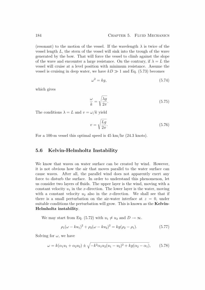
184 Chapter 5. Fluid Mechanics
(resonant) to the motion of the vessel. If the wavelength λ is twice of thevessel length L, the stern of the vessel will sink into the trough of the wavegenerated by the bow. That will force the vessel to climb against the slopeof the wave and encounter a large resistance. On the contrary, if λ = L thevessel will cruise at a level position with minimum resistance. Assume thevessel is cruising in deep water, we have kD À 1 and Eq. (5.73) becomes
ω2 = kg, (5.74)
which gives
ω
k=
√λg
2π. (5.75)
The conditions λ = L and v = ω/k yield
v =
√Lg
2π. (5.76)
For a 100-m vessel this optimal speed is 45 km/hr (24.3 knots).
5.6 Kelvin-Helmholtz Instability
We know that waves on water surface can be created by wind. However,it is not obvious how the air that moves parallel to the water surface cancause waves. After all, the parallel wind does not apparently exert anyforce to disturb the surface. In order to understand this phenomenon, letus consider two layers of fluids. The upper layer is the wind, moving with aconstant velocity u1 in the x-direction. The lower layer is the water, movingwith a constant velocity u2 also in the x-direction. We shall see that ifthere is a small perturbation on the air-water interface at z = 0, undersuitable conditions the perturbation will grow. This is known as the Kelvin-Helmholtz instability.
We may start from Eq. (5.72) with u1 6= u2 and D →∞.
ρ1(ω − ku1)2 + ρ2(ω − ku2)
2 = kg(ρ2 − ρ1). (5.77)
Solving for ω, we have
ω = k(α1u1 + α2u2)±√−k2α1α2(u1 − u2)2 + kg(α2 − α1), (5.78)

5.7. The Reynolds number 185
where
α1 =ρ1
ρ1 + ρ2
, α2 =ρ2
ρ1 + ρ2
. (5.79)
If ω has an imaginary part, u1z and u2z which are proportional to ei(kx−ωt) willgrow exponentially with time from an arbitrarily small initial perturbation.This occurs when
−k2α1α2(u1 − u2)2 + kg(α2 − α1) < 0. (5.80)
That is
k >g(α2 − α1)
α1α2(u1 − u2)2. (5.81)
Eq. (5.81) explains why low speed wind will only excite ripples of shortwavelength. It is interesting to know that even if the two fluids are identical(α1 = α2), the Kelvin-Helmholtz instability still exists. The instability canbe suppressed by viscosity when the velocity difference is small. That iswhy adding soluble polymers to water circulation systems can increase pumpefficiency by suppressing instabilities that cost energy.
5.7 The Reynolds number
In a system governed by the Navier-Stokes equation, instabilities that leadto turbulence may occur because the term (u · ∇)u is highly nonlinear. Theinstabilities can be suppressed by the diffusive term µ∇2u which tends tosmooth out the spatial variation of u. The crucial point is how large µ is,comparing with other parameters of the system. In Section 4.5 we have seenthat the range of action for diffusion within time t is on the order of
√Dt.
Hence for diffusion to be effective in smoothing out the spatial variation ofdensity,
√Dt must be comparable to the length scale l0 of the system. Let
us write the Navier-Stokes equation in the following form,
∂u
∂t+ (u · ∇)u = −∇P
ρm
+µ
ρm
∇2u + F (5.82)
where ρm is the mass density. By analogy, for viscosity to be effective in
smoothing out the spatial variation of u,√
µt/ρm must be comparable to l0.If the velocity scale of the system is u0, then the time scale of the system is

186 Chapter 5. Fluid Mechanics
l0/u0. Thus it is reasonable to imagine that under the following condition,viscosity is likely to suppress instabilities.
õl0
ρmu0
≈ l0. (5.83)
In a dimensionless form, this condition is equivalent to
1
R≡ µ
ρmu0l0≈ 1, (5.84)
where R is known as the Reynolds number. Instabilities occur usuallywhen R exceeds a few thousands.
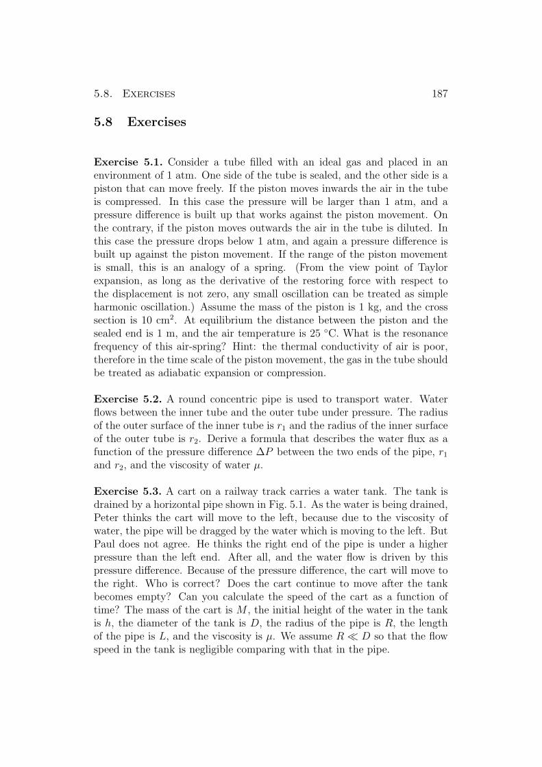
5.8. Exercises 187
5.8 Exercises
Exercise 5.1. Consider a tube filled with an ideal gas and placed in anenvironment of 1 atm. One side of the tube is sealed, and the other side is apiston that can move freely. If the piston moves inwards the air in the tubeis compressed. In this case the pressure will be larger than 1 atm, and apressure difference is built up that works against the piston movement. Onthe contrary, if the piston moves outwards the air in the tube is diluted. Inthis case the pressure drops below 1 atm, and again a pressure difference isbuilt up against the piston movement. If the range of the piston movementis small, this is an analogy of a spring. (From the view point of Taylorexpansion, as long as the derivative of the restoring force with respect tothe displacement is not zero, any small oscillation can be treated as simpleharmonic oscillation.) Assume the mass of the piston is 1 kg, and the crosssection is 10 cm2. At equilibrium the distance between the piston and thesealed end is 1 m, and the air temperature is 25 C. What is the resonancefrequency of this air-spring? Hint: the thermal conductivity of air is poor,therefore in the time scale of the piston movement, the gas in the tube shouldbe treated as adiabatic expansion or compression.
Exercise 5.2. A round concentric pipe is used to transport water. Waterflows between the inner tube and the outer tube under pressure. The radiusof the outer surface of the inner tube is r1 and the radius of the inner surfaceof the outer tube is r2. Derive a formula that describes the water flux as afunction of the pressure difference ∆P between the two ends of the pipe, r1
and r2, and the viscosity of water µ.
Exercise 5.3. A cart on a railway track carries a water tank. The tank isdrained by a horizontal pipe shown in Fig. 5.1. As the water is being drained,Peter thinks the cart will move to the left, because due to the viscosity ofwater, the pipe will be dragged by the water which is moving to the left. ButPaul does not agree. He thinks the right end of the pipe is under a higherpressure than the left end. After all, and the water flow is driven by thispressure difference. Because of the pressure difference, the cart will move tothe right. Who is correct? Does the cart continue to move after the tankbecomes empty? Can you calculate the speed of the cart as a function oftime? The mass of the cart is M , the initial height of the water in the tankis h, the diameter of the tank is D, the radius of the pipe is R, the lengthof the pipe is L, and the viscosity is µ. We assume R ¿ D so that the flowspeed in the tank is negligible comparing with that in the pipe.

188 Chapter 5. Fluid Mechanics
Fig. 5.1: Draining a tank.
Fig. 5.2: A balloon attached to an accelerating boxcar by a thread.
Exercise 5.4. A uniform solid plastic ball of density 0.5 g/cm3 is floatingon the surface of a water tank. Assume water is incompressible. If theatmosphere pressure is increased at a constant temperature, the volume of theball submerged in the water (1) increases, (2) decreases, (3) does not change.Choose your answer and explain why.
Exercise 5.5. A sealed boxcar is gliding down a slope with accelerationa = g sin θ as shown in Fig. 5.2, where g is the free-fall acceleration at thesurface of the Earth and θ is the angle of the slope. A balloon filled withhelium is attached to the floor by a thin thread. What is the angle φ betweenthe thread and the normal vector of the floor? You may not need the followingdata. But we provide them anyway in case you complain. The density of theair is 1.143 g/l. The density of helium in the balloon is 0.18 g/l. The volumeof the balloon is 10 l, and the weight of the balloon when empty is 4 g.
Exercise 5.6. An hourglass is made by welding the tips of two cone-shapedglass bottle together. The full angle of the cone is 30 and the height of eachcone is 10 cm. The neck connecting the two bottles has an inner diameter

5.8. Exercises 189
Fig. 5.3: Mechanical coupling by viscous fluid.
of 2 mm. The lower bottle is filled with tiny teflon balls whose diameter ismuch smaller than 2 mm. Now we flip the hourglass. How long does it takefor 7/8 of the teflon balls to flow into the lower bottle? In this problem weassume the teflon balls collectively behave like an incompressible fluid, andthe gap between the balls allows air to pass from the lower bottle to theupper bottle. We also assume the teflon balls are slippery enough so thatthe surface of the “fluid” remains flat all the time.
Exercise 5.7. Consider a shaft of radius r positioned at the center of arotating tube of length l as shown in Fig. 5.3. The inner radius of the tubeis R, and the angular velocity of the tube is ω. A viscous fluid of viscosity µis sealed in the space between the shaft and the tube. To prevent the shaftfrom rotating together with the tube, how much toque must be applied tothe shaft? In this exercise we ignore the viscous force from the end caps ofthe tube.
Exercise 5.8. It is well-known that the gravitational force from the Moon isthe major cause of the tidal wave observed twice a day. However, because theEarth is spinning and the tidal wave can only propagate with a finite speed,the tidal wave is not synchronized with the motion of the Moon. Assumethe Moon moves circularly in the equatorial plane of the Earth, and assumethere is no land on the surface of the Earth to interfere with the tidal-wavepropagation. If the wave length of the tidal wave is much larger than thedepth of the sea, how deep the sea must be for the tidal wave to synchronizewith the motion of the Moon? In this exercise we assume the curvature ofthe Earth’s surface is negligibly small.

190 Chapter 5. Fluid Mechanics

Chapter 6
Electrostatics
6.1 Gauss’ Law
From Coulomb’s law, the electric field at r produced by a charge densitydistribution ρ(r′) is
E(r) =1
4πε0
∫ρ(r′)
r− r′
|r− r′|3 d3r′, (6.1)
and the force acted on a charge density distribution by an external electricfield is
F =∫
ρ(r)E(r) d3r. (6.2)
Since
∇ 1
|r− r′| = − r− r′
|r− r′|3 , (6.3)
Eq. (6.1) can also be written as
E(r) = − 1
4πε0
∇∫ ρ(r′)|r− r′| d
3r′ = −∇φ(r), (6.4)
where
φ(r) =1
4πε0
∫ ρ(r′)|r− r′| d
3r′ (6.5)
191

192 Chapter 6. Electrostatics
is the electric potential. Mathematically Eq. (6.1) or (6.5) are not conve-nient to use because they involve integration all over the space. Moreover, ifthe charge distribution changes with time, because the electric field cannotchange instantly with the motion of the charges, the change of the electricfield will be delayed by |r− r′|/c. Namely,
E(r, t) =1
4πε0
∫ρ(r′, t′)
r− r′
|r− r′|3 d3r′, (6.6)
where t′ = t − |r − r′|/c. This further complicates the calculation. It turnsout that the 1/r2 dependence on the Coulomb force allows us to write a muchsimpler mathematical equation for the electric field, which is known as theGauss’ law.
Let us start by calculating the divergence of the electric field Ep producedby a single point charge q. From Eq. (1.343), it can be readily seen that
∇ · r
|r|3 = 0, (6.7)
everywhere except at r = 0, where the equation is undefined, therefore ∇ ·Ep = 0 except at r = 0. Consider the surface integral
∫
SEp · da,
where S is an arbitrary surface enclosing the charge. Imagine cutting thevolume enclosed by S into two parts V1 and V2. The first part V1 containsthe charge, and the second part V2 does not. The surface S is also dividedcorrespondingly into two surfaces S1 and S2. Let us denote H the interfacesurface between V1 and V2, then S1 + H encloses V1 and S2 + H encloses V2.We have
∫
SEp · da =
∫
S1+HEp · da +
∫
S2+HEp · da, (6.8)
because the surface integral at H cancels. Because ∇ ·Ep = 0 everywhere inV2, by Gauss’ theorem Eq. (1.322) the second term on the right-hand side ofEq. (6.8) is zero. Hence we have
∫
SEp · da =
∫
S1+HEp · da, (6.9)
This means we can deform the surface S successively to a small sphere aroundthe charge without changing the surface integral. Namely
∫
SEp · da =
∫
σEp · da, (6.10)

6.1. Gauss’ Law 193
where σ represents a sphere of radius r in which the charge sits at the center.But
∫
σEp · da =
q
ε0
, (6.11)
hence∫
SEp · da =
q
ε0
, (6.12)
for any surface enclosing the charge.
Now consider a group of charges enclosed by S. Since the field E producedby a group of charges is the superposition of that produced by each individualcharge, we have
∫
SE · da =
1
ε0
∫
Vρ(r) d3r. (6.13)
This is the integral form of the Gauss’ law. Using Gauss’ theorem, we have∫
V∇ · E d3r =
∫
SE · da =
1
ε0
∫
Vρ(r) d3r. (6.14)
Since V can be an arbitrarily small region, we have
∇ · E =ρ
ε0
. (6.15)
This is the differential form of the Gauss’ law. In terms of the electric po-tential, Gauss’ law is written as
−∇2φ =ρ
ε0
. (6.16)
Using Gauss’ law, we can prove the shell theorems easily. Let us considera sphere of uniform charge density. The radius of the sphere is R, and thetotal charge on the sphere is q. Let us choose the center of the sphere to bethe origin. By symmetry at position r the field is in the direction of r andonly a function of r. If r > R,
∫
SE · da = E(r)4πr2 =
q
ε0
, (6.17)
where S is a sphere centered at the origin with radius r. In other words
E(r) =1
4πε0
q
r2. (6.18)

194 Chapter 6. Electrostatics
This is the same as the case in which all the charge is put at the origin. Incontrast, if r < R there is no charge enclosed in the surface, hence E(r) = 0.
We can use Gauss’ law to calculate the electric field produced by chargedistributions that have high symmetries. For example, for charges uniformlydistributed on a infinite long line along the z-axis, by symmetry the electricfield is in the horizontal radial direction and is a function of r only. Let uschoose the surface of integration to be that of a cylinder along the z-axis,with radius r and length L. Gauss’ law yields
E(r)2πrL =ρlL
ε0
, (6.19)
where ρl is the line charge density. Hence
E(r) =ρl
2πε0r. (6.20)
Similarly, one can prove that the electric field produced by charges ona infinitely extended sheet is a constant. Again, by symmetry the electricfield is normal to the sheet and is only a function of the distance d to thesheet. By choosing the surface of integration to be that of a rectangular boxenclosing a rectangular area A of the sheet, Gauss’ law yields
E(d)2A =ρsA
ε0
, (6.21)
where ρs is the line charge density. Therefore
E(d) =ρs
2ε0
, (6.22)
which is a constant.
6.2 Electric Dipole
The simplest charge distribution beyond a single point charge or an uniformdistribution is the electric dipole. An electric dipole is formed by two chargesof opposite signs separated by a small distance. The electric field producedby an electric dipole at the origin is
E(r) = − q
4πε0
∇[
1
|r− d/2| −1
|r + d/2|
]. (6.23)

6.2. Electric Dipole 195
Consider the Taylor expansion of 1/|r− r′| around r for the case |r′| ¿ |r|.1
|r− r′| =1
r+∇
(1
r
)· (−r′) + . . .
=1
r+
r · r′r3
+ . . . (6.24)
At a distance r much larger than d, the first term of the Taylor expansion ofEq. (6.23) is
E(r) = − 1
4πε0
∇(p · r
r3
), (6.25)
where p = qd is called the electric dipole moment. For a charge distribu-tion centered around the origin, the definition of the dipole moment can begeneralized to
p ≡∫
r′ρ(r′) d3r′. (6.26)
Applying Eq. (6.24) to Eq. (6.5), we have
φ(r) =1
4πε0
[1
r
∫ρ(r′) d3r′ +
r
r3·∫
r′ρ(r′) d3r′ + . . .]
=1
4πε0
(q
r+ p · r
r3+ . . .
). (6.27)
The first term on the right-hand side is the monopole potential, and thesecond term is the dipole potential, which agrees with Eq. (6.25). For p inthe z-direction, Eqs. (6.25) and (1.339) gives
E(r) = − 1
4πε0
(∂
∂rr +
1
r
∂
∂θθ
) (p cos θ
r2
), (6.28)
hence
Er(r) =1
4πε0
2p cos θ
r3,
Eθ(r) =1
4πε0
p sin θ
r3,
Eφ(r) = 0. (6.29)
Consider a static charge distribution centered around the origin in anexternal field. If the length scale of variation of the external field is much

196 Chapter 6. Electrostatics
larger than the size of the charge distribution, the force experienced by thecharge distribution is
Fi =∫
ρ(r)Ei(r) d3r ≈∫
ρ(r)
[Ei(0) +
∂Ei
∂rj
rj
]d3r. (6.30)
If the net charge is zero, the term involving Ei(0) is zero, and the terminvolving ∂Ei/∂rj is the dipole force.
Fi =∂Ei
∂rj
pj, (6.31)
or
F = (p · ∇)E. (6.32)
Using the vector identity
∇(a · b) = (a · ∇)b + (b · ∇)a + a× (∇× b) + b× (∇× a) (6.33)
and noting that p is a constant vector and ∇×E = −∇×∇φ = 0, we have
F = ∇(p · E). (6.34)
The potential energy stored in the dipole is
U = −∫
F · ds = −∫∇(p · E) · ds = −p · E. (6.35)
The torque experienced by the charge distribution is
τ =∫
ρ(r)r× E(r) d3r ≈∫
ρ(r)r× E(0) d3r = p× E. (6.36)
6.3 Electric Polarization
Some molecules have a permanent dipole moment. They are called polarmolecules. Under an external field polar molecules will rotate until the dipolemoment is parallel to the field. For nonpolar molecules, the charge distri-bution can be deformed by the external field, such that the positive chargemoves in the direction of the field and the negative charge moves in the oppo-site direction. If the medium does not conduct electricity, the movement willnot continue, because after all the electrons cannot leave the atoms. But still,

6.3. Electric Polarization 197
the slight deformation will create a dipole moment again parallel to the field.Such dipoles are called induced dipoles. For a nonconducting medium let usdefine the electric polarization P to be the dipole moment per unit volume.From Eq. (6.25) it is seen that the electric polarization also contributes tothe electric potential. Namely,
φ(r) =1
4πε0
∫ [ρ(r′)|r− r′| + P(r′) · r− r′
|r− r′|3]
d3r′
=1
4πε0
∫ [ρ(r′)|r− r′| + P(r′) · ∇′ 1
|r− r′|
]d3r′. (6.37)
Assuming P = 0 at the boundary in the infinity, integration by parts gives
φ(r) =1
4πε0
∫ [ρ(r′)|r− r′| −
∇′ ·P(r′)|r− r′|
]d3r′. (6.38)
This is the potential produced by the charge distribution ρ−∇·P. Therefore,in a polarizable medium Gauss’ law becomes
∇ · E =1
ε0
(ρ−∇ ·P) . (6.39)
The electric displacement D is defined by
D = ε0E + P. (6.40)
We have
∇ ·D = ρ. (6.41)
In the linear regime the induced dipole moment is proportional to theexternal field, hence we may define χe such that
P = ε0χeE, (6.42)
where χe is called the electric susceptibility. In this case D is proportionalto E. The electric permittivity ε is defined by the following relation
D = εE, (6.43)
where
κe ≡ ε
ε0
= 1 + χe (6.44)

198 Chapter 6. Electrostatics
is called the dielectric constant or the relative electric permittivity. Substi-tuting Eq. (6.43) into Eq. (6.41), one obtains
∇ · E =ρ
κeε0
, (6.45)
or equivalently
∫
SE · da =
1
ε
∫
Vρ(r) d3r =
q
κeε0
. (6.46)
6.4 Capacitors
A capacitor is usually made of two narrowly spaced metal films, with a thinlayer of dielectric material sandwiched in between. Charges of opposite signscan be stored temporally on the two films without neutralizing each other.Due to the attractive force between the charges on the two films and therepulsive force between charges on the same film, the larger the film and thethinner the layer between them, the easier charges can be stored.
Let us model a capacitor by two infinitely large parallel plates with a smallgap between them. One surface is uniformly charged to +q and the other to−q. On both sides of the capacitor, because the electric field produced by auniformly charged sheet is a constant, the field produced by two uniformlycharged sheets of opposite sign is zero. Hence E = 0 everywhere exceptbetween the gap. To evaluate E between the gap, let us choose a rectangularbox that encloses a rectangular area A of only one sheet. Then the onlysurface on which E is nonzero is the surface between the gap. Gauss’ lawyields
EA =ρsA
ε0
, (6.47)
hence between the gap E is a constant. The voltage difference between theplates is simply V = Ed, and the charge is simply q = ρsA. The capacitanceC is defined by
C =q
V, (6.48)
hence
C =ε0A
d. (6.49)

6.4. Capacitors 199
Next we consider a capacitor made of two concentric cylinders with adielectric medium filling between them. The outer cylinder is charged to +qand the inner cylinder is charged to −q. Again the capacitance C is definedby C = q/V where V is the difference of the electrical potential between thetwo cylinders. By cylindrical symmetry, the electric field has only the radialcomponent. At radius r, we have
Er(r)2πrL =q
κeε0
, (6.50)
where L is the length of the cylinders. The potential difference is
V =∫ R2
R1
Er(r) dr =q
2πLκeε0
ln(
R2
R1
), (6.51)
where R1 and R2 are the radii of the inner and outer cylinders respectively.Hence
C =2πLκeε0
ln(R2/R1). (6.52)
In the limit R2 −R1 = d, d ¿ R1,
C =2πLκeε0
ln (1 + d/R1)≈ Aκeε0
d, (6.53)
where A = 2πR1L is the area of the conducting plate. This is the capacitanceof two parallel plates. Note that the capacitance is proportional to κe, hencefilling the gap with media of large dielectric constants is a common practicein manufacturing capacitors.
When a small amount of charge ∆q leaves the capacitor, it carries awaya small amount of energy equal to V ∆q. The total amount of energy thatcan be carried away from a capacitor of charge Q is
E =∫ Q
0V (q) dq =
∫ Q
0
Q− q
Cdq
=Q2
2C=
CV 2
2=
QV
2. (6.54)

200 Chapter 6. Electrostatics
6.5 Exercises
Exercise 6.1. 12 resistive wires are employed to construct the frame of acube. The resistance of each wire is R. If we connect one corner of the cubeto the ground and its diagonal corner to a voltage source of voltage V , whatis the current that flows out of the voltage source?
Exercise 6.2. Write down the electric potential produced by a charge +qat (d, 0, 0) and a charge −q at (−d, 0, 0). Show that the potential is zero onthe y-z plane.
Exercise 6.3. An infinitely large plane conductor is placed at the y-z plane.A charged particle carrying charge +q is placed on the x-axis with a distanced from the y-z plane. The charges on the conductor are attracted by thecharged particle, therefore they gather around the x-axis. Find the inducedsurface charge density as a function of the distance from the origin. Notethat if you know the electric field normal to the conductor, you can calculatethe surface charge density by Gauss’ law. Hint: On a conductor the electricpotential is a constant. Therefore the induced charge density must arrangeitself together with the charged particle at (d, 0, 0) to make the electric po-tential a constant. Because the conductor plane extends to infinity wherethe potential is zero, the constant potential must be zero. Therefore thesituation is similar to that of Exercise 6.2.
Exercise 6.4. Replace the infinitely large plane conductor in Exercise 6.3by a conducting sphere of radius R at the origin, where R < d. The sphere isconnected to the ground so that its potential is zero. Calculate the inducedsurface charge density on the sphere. Hint: You may try to replace thesphere by a negative charge −q′ at (d′, 0, 0) to make the electric potential atthe sphere equal to zero.
Exercise 6.5. Consider the circuit shown in Fig. 6.1. Each capacitor hasa capacitance of 1 µF, and R À 1 kΩ. In the beginning switches S1–S6
are closed and S7–S9 are open. At certain time switches S1–S6 are opened,and immediately after that switches S7–S9 are closed. What is the outputvoltage? If we close S10 now, how long does it take for the output voltage todrop to 1/e of its maximum value? A simplified version of the same circuitis shown in Fig. 6.2. Explain in words why the output pulse is practicallythe same as that in Fig. 6.1 if R À 1 kΩ. (If you can explain by calculation,it will even be better. But explaining in words is already acceptable.)

6.5. Exercises 201
Fig. 6.1: Maxbank high-voltage pulse generator.
Fig. 6.2: Maxbank high-voltage pulse generator, a simplified version.
Exercise 6.6. Two spherical electrodes of radius R separated by a distanced are buried deeply into a conducting material that extends to infinity inall directions. Assume R ¿ d. The conductivity of the material is σ. Oneelectrode is connected to a voltage source of +V and the other electrode isconnected to a voltage source of −V . What is the total current that flowsbetween the two electrodes? Use this method to measure the conductivity ofdistilled water, and compare it with the value on textbooks.
Exercise 6.7. A capacitor is made of two parallel conducting plates. Be-tween the plates is a plastic sheet with a dielectric constant κe > 1. If thecapacitor is charged by a battery and then disconnected, show that by remov-ing the plastic sheet, the energy stored in the capacitor is increased. Wheredoes the extra energy come from? In contrast, if the capacitor remains con-nected to the battery after it is charged, show that by removing the plasticsheet, the energy stored in the capacitor is decreased. Where does the energygo?
Exercise 6.8. In a conductor charges can move freely to form a steady-statedistribution ρs(r). At t = 0 if we set up a charge distribution ρ(r, 0) whichis different from ρs(r), the charge distribution will evolve into ρs(r) after a

202 Chapter 6. Electrostatics
while. Show that
ρ(r, t) = ρs(r) + [ρ(r, 0)− ρs(r)]e−λt.
where λ is related to the conductivity σ of the conductor. What is λ? Inthis exercise we assume the current associated with the change of chargedistribution is small enough such that the effect of inductance is negligible.
Exercise 6.9. In experimental physics it is important to confine the motionof ions in a small space in order to make the interaction time long enough.Show that it is impossible to make an ion trap by using only static electricfield.

Chapter 7
Magnetostatics
7.1 Ampere’s Law
In 1819 Oersted observed that magnetic flux can be produced by electric cur-rents. This was an important discovery, because it established the relationbetween electricity and magnetism, which appeared as two different phenom-ena before. By the experimental works of Biot and Savart, and later that ofAmpere, it was established that the magnetic-flux density B produced by acurrent density distribution J can be written as
B(r) =µ0
4π
∫J(r′)× r− r′
|r− r′|3 d3r′, (7.1)
and the force acted on a current density distribution by an external magnetic-flux density is
F =∫
J(r)×B(r) d3r. (7.2)
Since
∇ 1
|r− r′| = − r− r′
|r− r′|3 , (7.3)
from the vector identity
∇× (ψa) = ∇ψ × a + ψ∇× a, (7.4)
203

204 Chapter 7. Magnetostatics
Eq. (7.1) can be transformed into
B(r) = ∇× µ0
4π
∫ J(r′)|r− r′| d
3r′ − µ0
4π
∫ ∇× J(r′)|r− r′| d3r′. (7.5)
The second term on the right-hand side is zero because J(r′) does not dependon r. It then follows that
∇ ·B = 0, (7.6)
because ∇ · (∇× F) = 0 for any vector field F. Eq. (7.6) is consistent withthe fact that no magnetic charge has ever been found.
Similar to the transformation from Eq. (6.1) to Eq. (6.15), Eq. (7.1) canbe reduced to a much simpler form. By taking the curl of Eq. (7.1) and usingthe vector identity
∇× (a× b) = a(∇ · b)− b(∇ · a) + (b · ∇)a− (a · ∇)b, (7.7)
we have
∇×B(r) =µ0
4π
∫J(r′)∇ · r− r′
|r− r′|3 d3r′
− µ0
4π
∫[J(r′) · ∇]
r− r′
|r− r′|3 d3r′. (7.8)
For the first term on the right-hand side of Eq. (7.8), since
∇ · r− r′
|r− r′|3 = 0 (7.9)
except at r = r′, we may reduce the integration region to a small sphere σaround r without changing value of the integral.
∫J(r′)∇ · r− r′
|r− r′|3 d3r′ =∫
σJ(r′)∇ · r− r′
|r− r′|3 d3r′. (7.10)
In the limit where the radius of σ approaches zero, we have∫
σJ(r′)∇ · r− r′
|r− r′|3 d3r′ = J(r)∫
σ∇ · r− r′
|r− r′|3 d3r′. = 4πJ(r), (7.11)
where we obtain the second equality by Gauss’ theorem. For the second termon the right-hand side of Eq. (7.8), we note that
−∫
[J(r′) · ∇]r− r′
|r− r′|3 d3r′
= ∇∫
[J(r′) · ∇]1
|r− r′| d3r′
= ∇∫
J(r′) · ∇ 1
|r− r′| d3r′. (7.12)

7.1. Ampere’s Law 205
Because
∇ 1
|r− r′| = −∇′ 1
|r− r′| , (7.13)
where ∇′ means differentiation with respect to r′, we have
∇∫
J(r′) · ∇ 1
|r− r′| d3r′
= ∇∫
J(r′) · (−∇′)1
|r− r′| d3r′
= ∇∫ [
−∇′ · J(r′)|r− r′| +
∇′ · J(r′)|r− r′|
]d3r′
= ∇[−
∫
S
J(r′)|r− r′| · da +
∫ ∇′ · J(r′)|r− r′| d3r′
]. (7.14)
Assuming that there is no current at the boundary surface in the infinity,the first term on the right-hand side is zero. By the continuity equation∇′ · J = −∂ρ/∂t, we have ∇′ · J = 0 in the static case. Hence the secondterm on the right-hand side is also zero. Back to Eq. (7.8), we have
∇×B = µ0J. (7.15)
This is known as Ampere’s law. Its integral form is, according to Stokes’stheorem,
∮B · dl = µ0
∫
SJ · da. (7.16)
One may use Ampere’s law to calculate the magnetic flux density pro-duced by current distributions of high symmetry. Let us consider the mag-netic flux density produced by a current I on a infinitely long wire along thez-axis. At a distance r from the wire, by Eq. (7.1) we see that B is perpen-dicular to both the wire and r. Hence B has only the azimuthal component.Choosing the loop of integration to be a circle around the wire, Ampere’slaw yields
Bθ2πr = µ0I, (7.17)
hence
Bθ =µ0I
2πr. (7.18)

206 Chapter 7. Magnetostatics
Similarly, let us consider the magnetic flux density produced by a in-finitely large sheet of current distribution. Assuming the sheet is on the y-zplane with the current in the y-direction, and the observation point is at(d, y, z). Since the current distribution is independent of y and z, the mag-netic flux density at (d, y, z) is the same as that at (d, 0, 0). By Eq. (7.1),B at (d, 0, 0) must be perpendicular to both the y-axis and the positionvector dx, hence has only the z-component. Eq. (7.1) also tells us thatBz(−d, 0, 0) = −Bz(d, 0, 0). We may choose the loop of integration to be arectangular path in the z-x plane defined by the four corners (d, 0,−L/2),(d, 0, L/2), (−d, 0, L/2), and (−d, 0,−L/2). Ampere’s law yields
Bz(d)2L = µ0JsL, (7.19)
where Js is the surface current density. Therefore the magnetic flux densityproduced by a infinitely large sheet of current distribution is a constantµ0Js/2.
7.2 Lorentz Force
Since a current is nothing but a stream of moving charges, Eq. (7.2) gives theforce experienced by a group of moving charges in a magnetic flux density.
F =∫
J(r)×B(r) d3r
=∫
ρ(r)v(r)×B(r) d3r
=∑
i
qivi ×Bi, (7.20)
where qi and vi are the charge and velocity of the ith particle respectively,and Bi is the B-field at the location of the ith particle. Combining with theforce produced by the electric field, a moving charge experiences a force
F = q(E + v ×B). (7.21)
This is known as the Lorentz Force.

7.3. Force between Current Loops 207
7.3 Force between Current Loops
Consider the force between two current loops. According to Eqs. (7.1) and(7.2), the force is
F =∫
J1(r)×[µ0
4π
∫J2(r
′)× r− r′
|r− r′|3 d3r′]
d3r
=µ0
4πI1I2
∮ ∮ds×
(ds′ × r− r′
|r− r′|3)
, (7.22)
where we have used the relation
Ids = J d3r. (7.23)
By the vector identity Eq. (1.357), Eq. (7.22) can be reduced to
F =µ0
4πI1I2
[∮ ∮ds · r− r′
|r− r′|3 ds′ −∮ ∮
ds · ds′ r− r′
|r− r′|3]. (7.24)
Since
r− r′
|r− r′|3 = −∇ 1
|r− r′| , (7.25)
the first term on the right-hand side of Eq. (7.24) is zero. Hence
F = −µ0
4πI1I2
∮ ∮ds · ds′ r− r′
|r− r′|3 . (7.26)
7.4 Vector Potential
The vector potential A of the magnetic-flux density is defined by
B = ∇×A. (7.27)
This definition automatically satisfies the equation ∇ · B = 0. But how dowe know there is such a vector field satisfying Eq. (7.27)? Eq. (7.27) can beexplicitly written as
∂Az
∂y− ∂Ay
∂z= Bx,
∂Ax
∂z− ∂Az
∂x= By,
∂Ay
∂x− ∂Ax
∂y= Bz. (7.28)

208 Chapter 7. Magnetostatics
These are the three equations for the three components of A. However, since∇ ·B = 0 these three equations are not independent. It is easy to see that ifA satisfies the equation
∇×A = B, (7.29)
A′ = A+∇φ also satisfies the same equation, because ∇×∇φ = 0 for any φ.Therefore we must impose another condition to make the solution unique. Aconvenient condition to fix the solution is ∇·A = 0. By adding the condition∇ ·A = 0, we have enough equations to determine A. If ∇ ·A 6= 0, we canchoose φ such that
∇2φ = −∇ ·A. (7.30)
Then we have ∇ · A′ = ∇ · A + ∇2φ = 0. Since Eq. (7.30) is the same asthat for the electric potential Eq. (6.16), by Eq. (6.5) we see the appropriateφ to choose is
φ(r) =1
4π
∫ ∇′ ·A(r′)|r− r′| d3r′. (7.31)
To write out A explicitly, let us take the curl of Eq. (7.27). By the vectoridentity
∇× (∇×A) = ∇(∇ ·A)−∇2A, (7.32)
we have
∇2A = −∇×B. (7.33)
For each component of A, the equation is the same as that for the electricpotential Eq. (6.16), hence by Eq. (6.5) we have
A(r) =1
4π
∫ ∇′ ×B(r′)|r− r′| d3r′. (7.34)
The vector potential given by Eq. (7.34) satisfies ∇ ·A = 0, because
∇ ·A(r) =1
4π
∫[∇′ ×B(r′)] · ∇ 1
|r− r′| d3r′
=1
4π
∫[∇′ ×B(r′)] · (−∇′)
1
|r− r′| d3r′
= − 1
4π
∫∇′ ·
[∇′ ×B(r′)|r− r′|
]d3r′ +
1
4π
∫ ∇′ · [∇′ ×B(r′)]|r− r′| d3r′
= − 1
4π
∫
S
∇′ ×B(r′)|r− r′| · da +
1
4π
∫ ∇′ · [∇′ ×B(r′)]|r− r′| d3r′
= −µ0
4π
∫
S
J(r′)|r− r′| · da +
µ0
4π
∫ ∇′ · [J(r′)]|r− r′| d3r′. (7.35)

7.5. Magnetic Dipole 209
Assuming that there is no current at the boundary surface in the infinity, thefirst term on the right-hand side is zero. In the static case we have ∂ρ/∂t = 0.By the continuity equation it implies ∇ · J = 0. Hence the second term onthe right-hand side is also zero. Since ∇′ × B(r′) = µ0J(r′), Eq. (7.34) canbe written as
A(r) =µ0
4π
∫ J(r′)|r− r′| d
3r′. (7.36)
This is the same result we have already derived in Eq. (7.5). The symmetrybetween Eq. (6.5) and (7.36) reveals that using A to replace B in calculationhas the same advantage as using φ to replace E, as we shall see in thesubsequent sections.
7.5 Magnetic Dipole
Since an isolated magnetic charge has never been found, the simplest mag-netic structure is a magnetic dipole. A magnetic dipole can be defined bythe magnetic-flux density generated by a small current loop. Similar to theTaylor expansion of φ in Eq. (6.27), we may expand A in the following way:
Ai(r) =µ0
4π
[1
r
∫Ji(r
′) d3r′ +r
r3·∫
r′Ji(r′) d3r′ + . . .
]. (7.37)
By the vector identity
ri∂Jk
∂xk
=∂
∂xk
(xiJk)− ∂xi
∂xk
Jk =∂
∂xk
(xiJk)− Ji, (7.38)
which reads
ri∇ · J = ∇ · (riJ)− Ji, (7.39)
and the fact ∇ · J = 0, we have
∇ · (riJ) = Ji. (7.40)
Hence∫
Ji d3r =
∫∇ · (riJ)d3r =
∫
SriJ · da, (7.41)
where in the last step we have used Gauss’ theorem. For a localized currentdistribution, we may assume that J vanishes at some boundary surface. Then

210 Chapter 7. Magnetostatics
the first term on the right-hand side of Eq. (7.37) is zero. The second termon the right-hand side of Eq. (7.37) can be reduced by the vector identity
(r · r′)J = (r · J)r′ − r× (r′ × J). (7.42)
We shall first prove∫
(r · r′)J(r′) d3r′ = −∫
[r · J(r′)]r′ d3r′. (7.43)
From Eq. (7.40) one has∫
r′k∇′ · [r′iJ(r′)] d3r′ =∫
r′kJi(r′) d3r′. (7.44)
Using the identity
∇ · (ψa) = (a · ∇)ψ + ψ∇ · a (7.45)
we have∫
r′k∇′ · [r′iJ(r′)] d3r′ =∫∇′ · [r′kr′iJ(r′)] d3r′ −
∫r′iJ(r′) · (∇′r′k) d3r′
=∫
Sr′kr
′iJ(r′) · da′ −
∫r′iJ(r′) · (δlkel) d3r′
=∫
Sr′kr
′iJ(r′) · da′ −
∫r′iJk(r
′) d3r′. (7.46)
For a localized current distribution, we may assuming J = 0 at some bound-ary surface. Then the first term on the right-hand side vanishes, and fromEq. (7.40) we have
−∫
r′iJk(r′) d3r′ =
∫r′kJi(r
′) d3r′. (7.47)
Multiplying both sides by ri and summing over i, we have
−∫
rir′iJk(r
′) d3r′ =∫
riJi(r′)r′k d3r′, (7.48)
where the repeated index is by definition summed over. This is exactlyEq. (7.43). Integrating Eq. (7.42) and substituting Eq. (7.43) into it, weobtain
∫(r · r′)J(r′) d3r′ = −r× 1
2
∫r′ × J(r′) d3r′. (7.49)
With this identity, Eq. (7.37) is reduced to
A(r) = − µ0
4πr3r× 1
2
∫r′ × J(r′) d3r′. (7.50)

7.5. Magnetic Dipole 211
The magnetic moment is defined as
m =1
2
∫r′ × J(r′) d3r′, (7.51)
and
A =µ0
4π
m× r
r3. (7.52)
For m in the z-direction,
A =µ0
4π
m sin θ
r2φ. (7.53)
B = ∇×A and Eq. (1.350) gives
Br =µ0
4π
1
r2 sin θ
∂
∂θ
[r sin θ
(m sin θ
r2
)]=
µ0
4π
2m cos θ
r3,
Bθ = −µ0
4π
1
r sin θ
∂
∂r
[r sin θ
(m sin θ
r2
)]=
µ0
4π
m sin θ
r3. (7.54)
The field pattern is exactly the same as in Eq. (6.29), hence justifyingEq. (7.51) as the definition of magnetic dipole moment.
If a current I flows in a closed loop whose line element is dl, Eq. (7.51)becomes
m =I
2
∫r× dl. (7.55)
If the loop is in a plane,
∫r× dl = 2a, (7.56)
where a = |a| is the area enclosed by the loop, and the direction of a isnormal to the plane. Hence we have
m = Ia. (7.57)
If we replace J(r′) by ρ(r′)v(r′) in Eq. (7.51) and note that r′×v(r′) is simplythe angular momentum L divided by the mass m of the charges, we have
m =q
2mL. (7.58)

212 Chapter 7. Magnetostatics
Because the magnetic-flux density produced by a tiny magnet has the samepattern as Eq. (7.54), Eq. (7.58) suggests that magnetism originates fromthe angular momentum of electrons in atoms.
To find out the force and torque acted on a magnetic dipole, let us considerthe following function
Um(r) = −∫
J(r′ − r) ·A(r′) d3r′. (7.59)
Taking the gradient of both sides and using
∇(a · b) = (a · ∇)b + (b · ∇)a + a× (∇× b) + b× (∇× a), (7.60)
we have
∇Um(r) = −∫
[A(r′) · ∇]J(r′ − r) + A(r′)× [∇× J(r′ − r)]d3r′. (7.61)
Because J is a function of r′ − r, we can replace ∇ by −∇′ which operateson functions of r′.
∇Um(r) =∫
[A(r′) · ∇′]J(r′ − r) + A(r′)× [∇′ × J(r′ − r)]d3r′. (7.62)
Using Eq. (7.60) again, we have
∇Um(r) =∫∇′[J(r′ − r) ·A(r′)]d3r′
−∫
[J(r′ − r) · ∇′]A(r′) + J(r′ − r)× [∇′ ×A(r′)]d3r′. (7.63)
Let us examine the x′-component of the first term on the right-hand side.
∫ ∂
∂x′[J(r′ − r) ·A(r′)]dx′dy′dz′ =
∫[J(r′ − r) ·A(r′)]dy′dz′
∣∣∣∣x′=∞
x′=−∞. (7.64)
Assuming J = 0 at the boundary surface in the infinity, this term vanishes.The same is true for the other two components. Hence the first term on theright-hand side of Eq. (7.63) is zero. Using
∇ · (ψa) = (a · ∇)ψ + ψ∇ · a (7.65)
the second term on the right-hand side of Eq. (7.63) becomes∫
[J(r′ − r) · ∇′]Ai(r′) d3r′
=∫∇′ · [J(r′ − r)Ai(r
′)]− Ai(r′)[∇′ · J(r′ − r)] d3r′. (7.66)

7.5. Magnetic Dipole 213
The first term on the right-hand side can be reduced to a surface integral.Assuming J = 0 at the boundary surface in the infinity, this term is zero.The second term on the right-hand side is also zero because for static currentdensity distributions, ∇ · J = 0. Therefore we have
∇Um(r) = −∫
J(r′ − r)× [∇′ ×A(r′)] d3r′
= −∫
J(r′ − r)×B(r′) d3r′. (7.67)
From Eq. (7.2), we see that −∇Um(r) is the force experienced by the currentdensity distribution J(r′ − r). Hence in Eq. (7.59)
Um(r) = −∫
J(r′ − r) ·A(r′) d3r′ (7.68)
is the potential energy of a current density distribution J(r′ − r) in a fixedexternal field A(r′).
Next, we expand A in Eq. (7.59) to show the contribution of the magneticdipole in Um(0).
Um(0) = −∫
Ji(r′)Ai(r
′) d3r′
= −∫
[Ai(0) + r′ · ∇Ai(0)] Ji(r′) d3r′. (7.69)
By the vector identity
ri∇ · J = ∇ · (riJ)− Ji (7.70)
and the fact ∇ · J = 0, we have
∇ · (riJ) = Ji, (7.71)
hence∫
Ji d3r =
∫∇ · (riJ)d3r =
∫
SriJ · da, (7.72)
where in the last step we have used Gauss’ theorem. Assuming there is nocurrent at the boundary surface in the infinity, it is seen the first term onthe right-hand side of Eq. (7.69) vanishes. In the tensor notation we have
a× b = aibjεijk, (7.73)

214 Chapter 7. Magnetostatics
where εijk = 1 if the order of permutation for ijk is even, εijk = −1 if theorder of permutation is odd, and εijk = 0 if any two indices are the same.Define Ai
j ≡ ∂Ai/∂rj, in the tensor notation Eq. (7.69) becomes
Um(0) = −∫
r′jAijJi d
3r′. (7.74)
Using the identity εijkεlmk = δilδjm − δimδjl in Eq. (1.355), Eq. (7.47) can bewritten as
∫r′lJm d3r′ =
1
2
∫(r′lJm − r′mJl) d3r′
=1
2
∫r′iJj(δilδjm − δimδjl) d3r′
=1
2
∫r′iJjεijkεlmk d3r′. (7.75)
Multiplying both sides by Aαl , we have
∫Aα
l r′lJm d3r′ =1
2
∫r′iJjεijkA
αl εlmk d3r′. (7.76)
Eq. (7.51) is equivalent to
1
2
∫r′iJjεijk d3r′ = mk, (7.77)
where mk is the kth component of m, hence we have∫
Aαl r′lJm d3r′ = mkA
αl εlmk. (7.78)
Multiplying both sides by δmα, it becomes∫
Aαl r′lJα d3r′ = mkA
αl εlαk. (7.79)
Noting that the left hand side is∫
Aαl r′lJα d3r′ = −Um(0) and on the right-
hand side Aαl εlαk is simply the kth component of ∇×A = B. That is,
Um = −mkBk = −m ·B. (7.80)
The force acted on the current distribution is therefore
F = ∇(m ·B). (7.81)
To find out the torque τ acted on a magnetic dipole, we note that
τ ≈∫
r′ × [J(r′)×B(0)] d3r′
=∫
[r′ ·B(0)]J(r′) d3r′ −∫
[r′ · J(r′)]B(0) d3r′. (7.82)

7.6. Magnetization 215
By the same method we derive Eq. (7.49), namely replacing r by B(0), wecan show that
∫[B(0) · r′]J(r′) d3r′ = −B(0)× 1
2
∫r′ × J(r′) d3r′
= m×B(0), (7.83)
while by Eq. (7.47)
∫[r′ · J(r′)]B(0) d3r′ = B(0)
∫r′ · J(r′) d3r′ = 0. (7.84)
Therefore
τ = m×B. (7.85)
7.6 Magnetization
Some materials are made of atoms or molecules with a permanent magneticdipole moment. Under an external field the atoms or molecules may rotateto make their magnetic moment parallel to the field. Even without rotation,the current distribution can be deformed by the external field, as a resultthe magnetic moment changes. Let us define the magnetization M to be themagnetic dipole moment per unit volume. From Eqs. (7.50) and (7.51) it isseen that the magnetization also contributes to the vector potential. Namely,
A(r) =µ0
4π
∫ [J(r′)|r− r′| +
M(r′)× (r− r′)|r− r′|3
]d3r′. (7.86)
The magnetization term can be written as
∫ M(r′)× (r− r′)|r− r′|3 d3r′ =
∫M(r′)×
(∇′ 1
|r− r′|
)d3r′
=∫ ∇′ ×M(r′)
|r− r′| d3r′ −∫∇′ × M(r′)
|r− r′| d3r′, (7.87)
where we have used the vector identity ∇× (ψa) = ∇ψ × a + ψ∇× a. Thesecond term on the right-hand side can be reduced to surface integral byStokes’ theorem. Let us consider its z-component by defining a new vector
N(r′) =Mx(r
′)|r− r′| x +
My(r′)
|r− r′| y. (7.88)

216 Chapter 7. Magnetostatics
(∫∇′ × M(r′)
|r− r′| d3r′
)
z
=∫
[∇′ ×N(r′)] · zdxdydz
=∫ (∮
N(r′) · dl)
dz, (7.89)
where the line integral is over a loop at infinity on the x-y plane. AssumingM = 0 in the infinity, this term vanishes. From Eq. (7.34) we have
∇×B = µ0J + µ0∇×M. (7.90)
The magnetization thus plays the role of an effective current density
JM = ∇×M. (7.91)
The macroscopic field H called the magnetic field is defined by
H =B
µ0
−M. (7.92)
Then we have
∇×H = J. (7.93)
For some materials M is proportional to H, then we have
M = χmH, (7.94)
where χm is the magnetic susceptibility. In this case
B = µ0(χm + 1)H = κmµ0H = µH, (7.95)
where κm is called the relative permeability and µ the absolute permeability.

7.7. Exercises 217
7.7 Exercises
Exercise 7.1. Two charged particles carrying charges +q and −q are sep-arated by a distance d in the y-direction. They are also moving in thex-direction with the same velocity v. The mutual attraction force betweenthem is F when v = 0. At what v the mutual attraction between them isreduced to F/2?
Exercise 7.2. A solid metal cylinder rotating with angular velocity ω aboutits axis is put in a uniform magnetic field B parallel to its axis. The Lorentzforce and the centrifugal force push electrons to create a charge distribution.What is the charge distribution? If the charge distribution you obtainedcan be positive or negative everywhere, how would you explain the law ofcharge conservation? Hint: Since the charge cannot leave the cylinder, itmay accumulate on the surface.

218 Chapter 7. Magnetostatics
Chapter 8
Electrodynamics
8.1 Faraday’s Law
In 1831 Faraday discovered that an electric current can be induced in a closedwire loop by changing the magnetic flux that goes through the loop. Thisimportant discovery can be written in the following mathematical form:
E = − d
dt
∫B · da, (8.1)
where E is called the electromotive force, and the integration on the right-hand side covers the surface enclosed by the wire loop. Faraday observedthat the relation between E and the induced current I simply follows theOhm’s law:
E = IR, (8.2)
where R is the resistance of the wire. Hence E can be interpreted as theresult of an induced electric field that drives the current. The directionof the electromotive force is such that the magnetic flux produced by theinduced current is opposite to the change of the magnetic flux. In otherwords, the induced current works against the change of the magnetic flux.This is known as Lenz’ law.
Maxwell recognized that Eq. (8.1) is more general than it appears. Be-cause it does not require a wire to define the electric field, and in fact an
219

220 Chapter 8. Electrodynamics
electric field can be defined even in vacuum, Maxwell rewrote Eq. (8.1) inthe following form which is independent of the presence of a wire.
∮E · ds = − d
dt
∫B · da. (8.3)
This is an important step in the development of electrodynamics, because itreveals directly that an electric field can be induced by a changing magneticflux, even in vacuum. For the case of a static loop, by using the Stoke’stheorem Eq. (8.3) can be written in the differential form
∇× E = −∂B
∂t. (8.4)
But what about a moving wire loop? In Faraday’s experiments the chang-ing magnetic flux may arise from a wire loop moving in a static magneticflux density distribution. How should we describe such cases by Eq. (8.3)? Itturns out that as a wire moves relative to a magnetic flux density, a chargeq in the wire will also experience a force proportional to qv × B, in addi-tional to the electric force qE, as shown in Eq. (7.21). Consider a closed loopmoving at velocity v. If the loop has a fixed shape, then every point on theloop labeled by the position vector r must move at the same velocity. In thiscase v is independent of r. We may apply the convective derivative to theright-hand side of Eq. (8.1).
dB
dt=
∂B
∂t+ (v · ∇)B =
∂B
∂t+∇× (B× v) + v(∇ ·B). (8.5)
Substituting into Eq. (8.3), for a static B-field we have
∮E · ds = −
∫∇× (B× v) · da. (8.6)
Using the Stoke’s theorem, we have
∮E · ds =
∫(v ×B) · ds. (8.7)
This establishes the fact that in the case of a moving wire loop, the electro-motive force is nothing but the Lorentz force. Because v × ds is the areaswept by the line element ds per unit time, we have
∮(v ×B) · ds =
∮B · (ds× v) = −
∫B · ∂(da)
∂t. (8.8)

8.2. Maxwell Equations 221
Substituting back into Eq. (8.7), we have
∮E · ds = −
∫B · ∂(da)
∂t. (8.9)
For a loop of fixed shape the area enclosed by the loop does not change,hence we have
∫ ∂(da)
∂t=
∂
∂t
∫da = 0. (8.10)
If B is uniform, the right-hand side of Eq. (8.9) vanishes. However, if B isnot uniform, the right-hand side of Eq. (8.9) does not vanish because eachpoint of integration is weighted by a different B. This is the electromotiveforce induced by a loop moving in a static B field. The change of flux arisesfrom the change of the surface of integration.
8.2 Maxwell Equations
Let us summarize the four laws we have learned that govern the electromag-netic interactions.Gauss’ law:
∇ ·D = ρ. (8.11)
Ampere’s law:
∇×H = J. (8.12)
Faraday’s law:
∇× E = −∂B
∂t. (8.13)
and because no magnetic charge has ever been found, we have
∇ ·B = 0. (8.14)
Among these laws, Ampere’s law is valid only for static cases. By applying∇·on both sides of Eq. (8.12), it leads to ∇·J = 0. This cannot be right for thegeneral case because the conservation of charge requires that ∇·J+∂ρ/∂t =0. Therefore Maxwell modified Eq. (8.12) to make it consistent with thecontinuity equation. The modification is done by adding JD = ∂D/∂t on the
222 Chapter 8. Electrodynamics
right-hand side of Eq. (8.12), where JD ≡ ∂D/∂t is called the displacementcurrent. This is known as the Ampere-Maxwell law:
∇×H = J +∂D
∂t. (8.15)
These equations are now called the Maxwell equations collectively.
The need to introduce JD in Ampere’s law can also be seen in Eq. (7.8).By Eq. (7.14), the second term on the right-hand side of Eq. (7.8) is
∇∫ µ0
4π
∇′ · J(r′)|r− r′| d3r′
=µ0
4π∇
∫ [−∂ρ(r′)
∂t
]1
|r− r′| d3r′
=µ0
4π
∂
∂t
∫ρ(r′)
r− r′
|r− r′|3 d3r′
= µ0ε0∂E
∂t. (8.16)
Therefore Eq. (7.15) should be
∇×B = µ0J + µ0ε0∂E
∂t. (8.17)
In a polarizable and magnetizable medium it becomes Eq. (8.15).
Substituting B = ∇×A into Faraday’s law, we have
∇×(E +
∂A
∂t
)= 0. (8.18)
This allows us to define a scalar potential φ by
−∇φ = E +∂A
∂t, (8.19)
or
E = −∇φ− ∂A
∂t. (8.20)
The vacuum forms of Eqs. (8.11) and (8.15) are
∇ · E =ρ
ε0
, (8.21)
∇×B = µ0
(J + ε0
∂E
∂t
). (8.22)

8.2. Maxwell Equations 223
Substituting Eq. (8.20) into Eq. (8.21), we obtain
∇2φ +∂
∂t(∇ ·A) = − ρ
ε0
. (8.23)
Substituting B = ∇×A and Eq. (8.20) into Eq. (8.22), we obtain
∇(∇ ·A)−∇2A = µ0J−∇(µ0ε0
∂φ
∂t
)− µ0ε0
∂2A
∂t2, (8.24)
where ∇×∇×A = ∇(∇ ·A)−∇2A. That is,
∇2A− µ0ε0∂2A
∂t2−∇
(µ0ε0
∂φ
∂t+∇ ·A
)= −µ0J. (8.25)
We have already mentioned that the equation B = ∇ ×A is not sufficientto determine A uniquely. The three components of the equation are notindependent because ∇ · B = 0. This allows us to impose an additionalcondition on A. For static cases we used to choose ∇ ·A = 0, but now if wechoose
µ0ε0∂φ
∂t+∇ ·A = 0, (8.26)
Eqs. (8.23) and (8.25) can be simplified to the following form:
∇2φ− µ0ε0∂2φ
∂t2= − ρ
ε0
. (8.27)
∇2A− µ0ε0∂2A
∂t2= −µ0J. (8.28)
Eqs. (8.26), (8.27), and (8.28) are equivalent to the Maxwell equations.
In a medium whose polarization and magnetization response linearly tothe electromagnetic field, Eqs. (8.11) and (8.12) become
∇ · E =ρ
ε, (8.29)
∇×B = µ
(J + ε
∂E
∂t
), (8.30)
and Eqs. (8.26), (8.27), and (8.28) become
µε∂φ
∂t+∇ ·A = 0, (8.31)
∇2φ− µε∂2φ
∂t2= −ρ
ε, (8.32)
∇2A− µε∂2A
∂t2= −µJ. (8.33)

224 Chapter 8. Electrodynamics
8.3 Electromagnetic Waves
Before Maxwell, E and B are thought of as mathematical instruments forcalculating the interactions between charges and currents. It is more conve-nient to calculate first E and B from the charge and current sources thenuse them to calculate the force experienced by a test charge or current. ButEqs. (8.27) and (8.28) reveal that even if there is no charge and current, Eand B can exist in the form of electromagnetic waves. Of course, one canargue that the existence of the wave equation does not guarantee its solution,because after all, there must be an initial disturbance of charges or currentsat some place to produce the wave, just like a pendulum will not oscillate byitself; there must be someone to give it an initial push. Such kinds of debatein point of view can become philosophical. In the end, it is hard to deny theadvantage of treating E and B as real physical quantities. This is because interms of source charges and currents, the interaction is distributed. Namely,as we shall see in Section 8.5, the force between a test charge q and a chargedistribution ρ(r′, t′) is
F(r, t) =q
4πε0
∫ρ(r′, t′)
r− r′
|r− r′|3 d3r′, (8.34)
where t′ = t − |r − r′|/c and c is the speed of propagation for the electro-magnetic disturbance, and the force between a current I of length dl and acurrent distribution J(r′, t′) is
dF(r, t) =µ0Idl
4π×
∫J(r′, t′)× r− r′
|r− r′|3 d3r′. (8.35)
In contrast, in terms of E and B, the interaction is simply the Lorentz forceequation
F(r, t) = ρE(r, t) + J×B(r, t), (8.36)
where F(r, t) is the force per unit volume. The interaction is local, meaningthat only physical quantities at r is involved. This is why it is advantageousto treat electromagnetic fields as real physical quantities such that we donot always need to know where the sources are and what they are doing.As a matter of fact, no one has ever looked at a charge as a banana inone’s hand; we know the existence of charges only through their interactionwith other charges. Therefore, in physics the interaction between variousphysical quantities is the only thing we are sure about. In this point of viewelectromagnetic fields are physically as real as charges and currents.

8.3. Electromagnetic Waves 225
When there is no charge or current, Eqs. (8.32) and (8.33) become thewave equations. They show that even when locally there is no source ofthe electromagnetic field, the electromagnetic field can still exist as waves.The prediction of the existence of electromagnetic waves is a great triumphof the Maxwell equations. It turns out that 1/
√µ0ε0, the phase velocity of
the electromagnetic wave, is the same as the speed of light. Hence Maxwellequations also suggested that light is a kind of electromagnetic waves.
The existence of electromagnetic waves can also be seen directly from theMaxwell equations without going through the scalar and vector potentials.By taking the curl of both sides of Eq. (8.13), we have
∇× (∇× E) = − ∂
∂t∇×B. (8.37)
Using µH = B and Eq. (8.15) to replace ∇×B, we have
∇× (∇× E) = ∇(∇ · E)−∇2E = −µ∂
∂t
(J +
∂D
∂t
). (8.38)
Using εE = D and Eq. (8.11)
∇2E− µε∂2E
∂t2=
1
ε∇ρ + µ
∂J
∂t. (8.39)
Similarly, taking the curl of both sides of Eq. (8.15) and using εE = D,µH = B, we have
∇× (∇×B) = µ∇× J + µε∂
∂t∇× E. (8.40)
Using Eq. (8.13) to replace ∇× E, we have
∇× (∇×B) = ∇(∇ ·B)−∇2B = µ∇× J− µε∂2B
∂t2, (8.41)
or
∇2B− µε∂2B
∂t2= −µ∇× J. (8.42)
When there is no charge or current, E and B can still exist as waves withphase velocity v = 1/
√µε in media and v = 1/
√µ0ε0 = c in vacuum.

226 Chapter 8. Electrodynamics
8.4 Radiation by Charge Acceleration
Let us look into the solutions of Eqs. (8.27) and (8.28). The equations areof the form
∇2φ(r, t)− 1
c2
∂2φ(r, t)
∂t2= −f(r, t). (8.43)
By expanding φ(r, t) and f(r, t) into a superposition of modes with timedependent amplitudes,
φ(r, t) =∑
k
a(k, t)uk(r), (8.44)
f(r, t) =∑
k
g(k, t)uk(r), (8.45)
we have
∑
k
[∇2uk(r)a(k, t)− 1
c2uk(r)a(k, t)
]= −∑
k
uk(r)g(k, t). (8.46)
For simplicity, let us choose uk(r) to be the Fourier components exp(ik · r).Then we have
∑
k
[−k2uk(r)a(k, t)− 1
c2uk(r)a(k, t)
]= −∑
k
uk(r)g(k, t). (8.47)
Because exp(ik · r) forms a complete orthonormal basis, we have
k2a(k, t) +1
c2a(k, t) = g(k, t). (8.48)
For each k, this is the equation of a driven harmonic oscillator. In realityany harmonic oscillator must have a damping factor, no matter how smallit is. Similarly we can add a damping term to Eq. (8.48) even though it isnegligibly small. The reason we keep it here is that it helps in the followingcalculation. With the damping term added Eq. (8.48) becomes
k2a(k, t) +γ
c2a(k, t) +
1
c2a(k, t) = g(k, t), (8.49)
where γ is a positive constant. For each k this is the same equation as that ofa driven harmonic oscillator, which has been solved in Eq. (3.11). Thereforewe may write out the solution directly. In the case γ → 0 we have
a(k, t) =c
k
∫
t>t′sin[ck(t− t′)]g(k, t′) dt′. (8.50)

8.5. Retarded Potentials 227
In the above analysis, we see that electromagnetic waves are driven bytime-varying charges and currents. If the electromagnetic radiation is pro-duced by currents in a charge neutral environment such as a metal wire, wehave ρ = 0. In this case we see J must be a function of time in order to pro-duce radiation (ω 6= 0). In other words, electromagnetic waves are producedby accelerating charges.
8.5 Retarded Potentials
According to Eq. (1.346), in the spherically symmetric case Eq. (8.27) be-comes
1
r2
∂
∂r
[r2∂φ(r, t)
∂r
]− 1
c2
∂2φ(r, t)
∂t2= −ρ(r, t)
ε0
. (8.51)
Let us change the variable to u(r, t) ≡ rφ(r, t), we have
1
r
[∂2u(r, t)
∂r2− 1
c2
∂2u(r, t)
∂t2
]= −ρ(r, t)
ε0
. (8.52)
For a point charge at r = 0, we have[∂2u(r, t)
∂r2− 1
c2
∂2u(r, t)
∂t2
]= 0, (8.53)
except for r = 0. The solution is
u(r, t) =∑
k
ak(t)eikr, (8.54)
where ak(t) satisfies the equation for the harmonic oscillator.
ak(t) + c2k2ak(t) = 0. (8.55)
Define ω ≡ ck, we have
u(r, t) =∑
k
ckei(kr−ωt) + dke
i(kr+ωt). (8.56)
At this point let us focus our attention only on the outgoing wave, then wechoose only the first term
u(r, t) =∑
k
ckei(kr−ωt). (8.57)
228 Chapter 8. Electrodynamics
Hence
φ(r, t) =∑
k
ckei(kr−ωt)
r. (8.58)
This is the outgoing-wave solution of Eq. (8.51) for r 6= 0 when the onlysource of φ is a point charge at r = 0. Let us expand ρ(r, t) into a Fourierseries,
−ρ(r, t)
ε0
= − 1
ε0
∑ω
ρ(r, ω)e−iωt (8.59)
and substitute it and Eq. (8.58) back into Eq. (8.51). We have
∑
k
cke−iωt
[∇2
(eikr
r
)+ k2 eikr
r
]= − 1
ε0
∑ω
ρ(r, ω)e−iωt. (8.60)
Since ω = ck, we may replace∑
k in Eq. (8.60) by∑
ω. Comparing coeffi-cients, we have
ck
[∇2
(eikr
r
)+ k2 eikr
r
]= − 1
ε0
ρ(r, ω). (8.61)
Since ρ(r, ω) = 0 except at r = 0, we may integrate the above equation overa small sphere σ with radius rσ around the origin.
ck
∫
σ
[∇2
(eikr
r
)+ k2 eikr
r
]d3r = − 1
ε0
∫
σρ(r, ω) d3r. (8.62)
The second term on the left-hand side approaches zero as rσ → 0 because∣∣∣∣∣∫
σ
eikr
rd3r
∣∣∣∣∣ ≤∫
σ
1
rd3r
=∫ rσ
04πrdr
= 2πr2σ. (8.63)
The first term can be reduced to a surface integral by Gauss’ theorem.
ck
∫
σ∇2
(eikr
r
)d3r
= ck
∫
σ∇ ·
[ik
eikr
rr + eikr∇
(1
r
)]d3r
= ck
∫
sσ
[ik
eikr
rr + eikr∇
(1
r
)]· da, (8.64)

8.5. Retarded Potentials 229
where sσ is the surface of σ. The first term on the right-hand side approacheszero as rσ → 0, because
∣∣∣∣∣∫
sσ
eikr
rr · da
∣∣∣∣∣ ≤1
rσ
4πr2σ (8.65)
The second term is equal to −4πck as rσ → 0, because
limrσ→0
eikrσ → 1, (8.66)
and
limrσ→0
∫
sσ
∇(
1
r
)· da = lim
rσ→0
∫
sσ
(−r
r2
)· da = −4π. (8.67)
Hence
ck =1
4πε0
∫
σρ(r′, ω) d3r′. (8.68)
Putting ck back into Eq. (8.58), we have
φ(r, t) =1
4πε0
∑
k
ei(kr−ωt)
r
∫
σρ(r′, ω) d3r′
=1
4πε0
1
r
∫
σ
∑
k
ρ(r′, ω)e−i(ωt−kr) d3r′
=1
4πε0
1
r
∫
σ
∑ω
ρ(r′, ω)e−iω(t−r/c) d3r′
=1
4πε0
∫
σ
ρ(r′, t′)r
d3r′, (8.69)
where t′ = t − r/c. Eq. (8.69) describes the scalar potential produced by atime-varying charge density at the origin. If there is charge density in otherlocations, by superposition of φ we have
φ(r, t) =1
4πε0
∫ ρ(r′, t′)|r− r′| d
3r′. (8.70)
This is called the retarded scalar potential. It describes the scalar potentialat (r, t) produced by a time-varying charge density at (r′, t′) with t′ = t −|r− r′|/c.
Similarly, we have the retarded vector potential
A(r, t) =µ0
4π
∫ J(r′, t′)|r− r′| d3r′ (8.71)
which describes the vector potential at (r, t) produced by a time-varyingcurrent density at (r′, t′) with t′ = t− |r− r′|/c.

230 Chapter 8. Electrodynamics
8.6 Energy Density of Electromagnetic Fields
For a static charge distribution in a static external electric field, the potentialenergy is
UE =∫
ρ(r)φ(r) d3r. (8.72)
Let us write ρ(r) = αn(r), where α is a scalar proportional constant. If φ(r)is established by the charge distribution itself, then φ(r) is also proportionalto α, namely φ(r) = αψ(r). The potential energy stored in the chargedistribution is the energy spent in building up the distribution as we let αincrease from 0 to its final value.
UE =∫ α
0αdα
∫n(r)ψ(r) d3r =
1
2
∫ρ(r)φ(r) d3r. (8.73)
Using the identity ∇ · (ψa) = ψ∇ · a + a · ∇ψ, we may write Eq. (8.73) in adifferent form:
UE =1
2
∫ρ(r)φ(r) d3r
=1
2
∫[∇ ·D(r)]φ(r) d3r
=1
2
∫∇ · [φ(r)D(r)] d3r− 1
2
∫D(r) · [∇φ(r)] d3r
=1
2
∫
Sφ(r)D(r) · da− 1
2
∫D(r) · [∇φ(r)] d3r
=1
2
∫D(r) · E(r) d3r, (8.74)
where we assume the surface integral of φ(r)D(r) at infinity vanishes. Theequivalence between Eq. (8.73) and Eq. (8.74) suggests that we may look atthe electric potential energy from two different points of view, one as theenergy stored in the charges in a potential field according to Eq. (8.73), theother as the energy stored in the field itself according to Eq. (8.74). Using theequation ∇·E = ρ/ε0, we may switch between these two points of view freely.If we allow the charges to move by themselves, the movement will reduce thepotential energy, and the difference will be converted to the kinetic energyof the charges. Conversely, if the kinetic energy of the charges is decreased,it is converted into potential energy described by Eq. (8.73), which can alsobe viewed as the energy stored in the electric fields according to Eq. (8.74).

8.6. Energy Density of Electromagnetic Fields 231
For a static current distribution in a static magnetic field, the situationis different. In Eqs. (7.59) and (7.67) we have shown that if the force experi-enced by a static current distribution in a static magnetic field is considered,the potential energy is
Um = −∫
J(r) ·A(r) d3r. (8.75)
However, since v×B is perpendicular to v, the magnetic field cannot changethe kinetic energy of the charges. Where does this potential energy come fromthen? It turns out that Eq. (8.75) does not account for the total change ofenergy, because it requires an external battery to maintain the static currentdistribution. As a current is moved across a magnetic field, the Lorentz forcewill generate an equivalent electromotive force as shown in Eq. (8.7). If theelectromotive force is anti-parallel to the current density, the external batterymust do extra work against this electromotive force. If the electromotive forceis parallel to the current density, the external battery can save work by usingthe electromotive force as part of the driving force. Therefore, the extrapower delivered by the battery for a current density J(r′ − r) is
P (I)(r) = −∫
E(I)(r′) · J(r′ − r) d3r′
= −∫
[v ×B(r′)] · J(r′ − r) d3r′
=∫
[J(r′ − r)×B(r′)] · v d3r′, (8.76)
where v is the velocity of the parallel-moving current density and E(I)(r′) isthe electric field induced by the Faraday’s law. The energy delivered withina time dt by the battery is therefore
P (I)(r) dt = dr ·∫
J(r′ − r)×B(r′) d3r′, (8.77)
where r is the parallel displacement of the current density distribution. Inother words, the energy Ub stored in the external battery has changed by
dUb = −dr ·∫
J(r′ − r)×B(r′) d3r′, (8.78)
That is
∇Ub(r) = −∫
J(r′ − r)×B(r′) d3r′, (8.79)
Comparing with Eq. (7.67), we see Um = Ub. The mechanical potentialenergy Um is simply the energy stored in the external battery.

232 Chapter 8. Electrodynamics
Let us investigate how much energy is needed to build up a static magneticfield. In this case we do not parallel-move the current density distribution.Instead, we increase the magnetic field while keeping the current densitydistribution fixed. The total power supplied by the external battery thatmaintains the current density distribution is
P = −∫
E(r) · J(r) d3r
=∫ [
∇φ +∂A
∂t
]· J d3r
=∫ [
∇ · (φJ)− φ∇ · J +∂A
∂t· J
]d3r. (8.80)
Assuming there is no current on the boundary surface in the infinity, the firstterm on the right-hand side is zero. The second term on the right-hand sideis also zero because ∇ · J = 0. Therefore
P =∫
J · ∂A
∂td3r. (8.81)
The total energy supplied by the battery to build up A(r) while maintainingJ(r) fixed is
UB =∫
J(r) ·A(r) d3r. (8.82)
To see more clearly the physical meaning of Eq. (8.82), let us rewriteEq. (8.76) in the following way.
P (I)(r) =∫
v · [J(r′ − r)×B(r′)] d3r′
= −∫
B(r′) · [J(r′ − r)× v] d3r′
= −∫∇′ ×A(r′) · [J(r′ − r)× v] d3r′
=∫∇′ · [J(r′ − r)× v]×A(r′) d3r′
−∫∇′ × [J(r′ − r)× v] ·A(r′) d3r′
=∫
S[J(r′ − r)× v]×A(r′) · da′
+∫∇× [J(r′ − r)× v] ·A(r′) d3r′. (8.83)
In the derivation we have used the facts that v does not depend on r or r′ and∇′ operated on J(r′−r) is equal to −∇ operated on J(r′−r). Assuming there

8.6. Energy Density of Electromagnetic Fields 233
is no current on the boundary surface in the infinity, the surface integrationin Eq. (8.83) is zero. Using the identity
∇× (J× v) = −v(∇ · J) + (v · ∇)J, (8.84)
and noting that ∇ · J = 0, we obtain
P (I)(r) =∫
[(v · ∇)J(r′ − r)] ·A(r′) d3r′. (8.85)
Because
dJ(r′ − r)
dt=
∂J
∂t+ (v · ∇)J(r′ − r) (8.86)
and ∂J/∂t = 0, Eq. (8.85) can be reduced to
P (I)(r) =∫ dJ(r′ − r)
dt·A(r′) d3r′. (8.87)
That is
P (I) =∫ dJ(r′)
dt·A(r′) d3r′. (8.88)
Combining Eqs. (8.81), (8.82), and (8.88), we see
dUB
dt=
∫ [dJ(r)
dt·A(r) + J(r) · ∂A(r)
∂t
]d3r
= P (I) + P. (8.89)
Therefore UB is the total energy supplied by the batteries to build up thecombination of J(r) and A(r). This energy can be thought of as the energystored in the configuration specified by J(r) and A(r).
Let us write J(r) = βj(r), where β is a scalar proportional constant.If A(r) is established by the current distribution itself, then A(r) is alsoproportional to β, namely A(r) = βa(r). The potential energy stored in thecurrent distribution is the energy spent in building up the distribution as welet β increase from 0 to its final value.
UB =∫ β
0βdβ
∫j(r) · a(r) d3r =
1
2
∫J(r) ·A(r) d3r. (8.90)

234 Chapter 8. Electrodynamics
Using ∇ · (a× b) = b · (∇× a)− a · (∇× b) and Gauss’ theorem, we have
UB =1
2
∫J(r) ·A(r) d3r
=1
2
∫[∇×H(r)] ·A(r) d3r
=1
2
∫∇ · [H(r)×A(r)] d3r +
1
2
∫H(r) · [∇×A(r)] d3r
=1
2
∫
S[H(r)×A(r)] · da +
1
2
∫H(r) · [∇×A(r)] d3r
=1
2
∫H(r) ·B(r) d3r, (8.91)
where we assume the surface integral of H(r)×A(r) vanishes at infinity.
Let us consider now the energy density of time-varying electromagneticfields. The increase rate of the mechanical energy of a system of chargedparticles can be written as
Pm =∑
i
Fi · vi =∑
i
qi [E(ri) + vi ×B(ri)] · vi
=∫
E(r) · J(r) d3r. (8.92)
Replacing J by using the Ampere-Maxwell law,
Pm =∫ [
E · (∇×H)− E · ∂D
∂t
]d3r. (8.93)
Using the vector identity
∇ · (a× b) = b · (∇× a)− a · (∇× b) (8.94)
and Faraday’s law, we have
Pm = −∫ [
∇ · (E×H)−H · (∇× E) + E · ∂D
∂t
]d3r
= −∫ [
∇ · (E×H) + H · ∂B
∂t+ E · ∂D
∂t
]d3r. (8.95)
Define
U ≡ 1
2(E ·D + B ·H), (8.96)

8.7. Inductors and Transformers 235
and
S ≡ E×H. (8.97)
For media with linear polarization and magnetization, we have
−E · J =∂U
∂t+∇ · S. (8.98)
This is known as the Poynting’s theorem, and S is called the Poyntingvector. Since the decrease of the mechanical energy must be equal to theincrease of the electromagnetic energy, Poynting’s theorem suggests that Uis the energy density of the electromagnetic field, and S is the energy fluxdensity.
8.7 Inductors and Transformers
Consider the interaction of two circuits fixed in space through Faraday’s law.The electromotive forces in the circuits are induced by the total magneticfluxes that go through the surfaces enclosed by the circuits. For each circuit,electromotive force arises from two contributions. One is the magnetic fluxgenerated by the current in the circuit itself, and the other is the magneticflux produced by the other circuit.
E1 = − d
dt
∫(B1 + B2) · da1, (8.99)
where E1 is the electromotive force induced in circuit 1, da1 is the surfaceelement of the surface enclosed by circuit 1, and B1 and B2 are the mag-netic flux densities generated by circuit 1 and circuit 2 respectively. UsingEq. (7.27), we have
E1 = − d
dt
∫∇× (A1 + A2) · da1. (8.100)
Applying the Stokes theorem, we have
E1 = − d
dt
∮(A1 + A2) · ds1. (8.101)
Substituting Eq. (7.36) in for the vector potentials, we have
E1 = −µ0
4π
d
dt
∮ (∫ J1(r′1)
|r1 − r′1|d3r′1 +
∫ J2(r2)
|r1 − r2| d3r2
)· ds1. (8.102)

236 Chapter 8. Electrodynamics
Note that J1(r′1) d3r′1 = I1ds
′1 and J2(r2) d3r2 = I2ds2. The replacement
leads to
E1 = −µ0
4π
(dI1
dt
∮ ∮ ds′1 · ds1
|r1 − r′1|+
dI2
dt
∮ ∮ ds2 · ds1
|r1 − r2|
). (8.103)
The self-inductance of circuit 1 is defined by
L11 =µ0
4π
∮ ∮ ds′1 · ds1
|r1 − r′1|, (8.104)
and the mutual inductance between circuit 1 and circuit 2 is defined by
L12 =µ0
4π
∮ ∮ ds2 · ds1
|r1 − r2| , (8.105)
In terms of self-inductance and mutual inductance, Eq. (8.103) can be writtenas
E1 = −L11dI1
dt− L12
dI2
dt. (8.106)
An inductor is a wire loop with a significant self-inductance. Accordingto Lenz’ law, the induced current works against the change of the magneticflux, therefore an inductor has a tendency of resisting the change of currentthat flows through it. In contrast to a capacitor, which stores energy in theelectric field, an inductor can be thought as a device that stores energy inthe magnetic field. Let us “charge up” an inductor by turning on the currentgradually from 0 to I. As the current is increased, an electric field builds upagainst the flow of the current. Between t and t + ∆t, the work done by theexternal device that drives the current is simply
∆w = ∆q∮
E · (−dl)
= I∆t
(L
dI
dt
). (8.107)
The minus sign in the first equality means the charge is transported againstthe E field. In other words, the motion of the charge is in the oppositedirection of the line element dl. In the limit of ∆t → 0,
dw = LI dI. (8.108)
Hence the energy stored in an inductor L is
w =∫
LI dI =LI2
2. (8.109)

8.7. Inductors and Transformers 237
We may also obtain the same result directly from Eq. (8.90). By replacingJd3r with Ids in Eqs. (8.90) and (7.36), Eq. (8.90) becomes
UB =1
2
∫J(r) ·A(r) d3r =
I
2
∮ds ·
[µ0
4π
∫ J(r′)|r− r′| d
3r′]
=I2
2
µ0
4π
∮ ∮ ds · ds′|r− r′| =
LI2
2. (8.110)
Inductors are commonly made of solenoids. Let us calculate the induc-tance of an infinitely long linear solenoid. Because inductance is related to themagnetic flux enclosed by the wire loop, we only need to calculate the B-fieldinside the solenoid. Let the axis of the solenoid be the z-axis. By Eq. (7.1) weknow that B can only have the z-component and the r-component, becauseJ is in the θ-direction. The symmetry between the +z and −z directionsmakes all the contributions to the r-component cancel. Therefore we onlyneed to calculate Bz. By cylindrical symmetry and translational symmetryin z, Bz can be a function of r only. Let us choose a rectangular loop of in-tegration that goes up along the z-axis and comes back parallel to the z-axisat a distance r from the z-axis. Ampere’s law yields Bz(0) = Bz(r), sincethe loop does not enclose any current. Therefore inside the solenoid Bz is aconstant. Using Eq. (7.1) in cylindrical coordinates, we can calculate Bz(0).Let R be the radius of the solenoid, we have
Bz =µ0
4π
∫ ∞
−∞Js2πR
R2 + z2
R√R2 + z2
dz
=µ0Js
2
∫ ∞
−∞1
[1 + (z2/R2)]3/2d
(z
R
). (8.111)
By a change of variable tan θ = z/R, the integral can be evaluated.
Bz =µ0Js
2
∫ ∞
−∞1
(1 + tan2 θ)3/2d (tan θ)
=µ0Js
2
∫ +π/2
−π/2cos θdθ
= µ0Js = µ0nI, (8.112)
where n is the number of turns per unit length. The electromotive force perunit length is
E = − d
dt(nBzA) = −µ0n
2AdI
dt, (8.113)

238 Chapter 8. Electrodynamics
hence the inductance per unit length is
L = µ0n2A, (8.114)
Another example of inductor is a toroid of rectangular cross section. As-sume the inner radius of the toroid is a and the outer radius is b, and theheight is h. Using Ampere’s law, the magnetic flux density at r is
Bθ(r)2πr = µ0NI, (8.115)
where N is the total number of turns. The magnetic flux is
φm =∫ b
a
µ0NI
2πrh dr =
µ0NIh
2πln
(b
a
). (8.116)
Since each turn picks up an E = −dφm/dt, the inductance is
L =µ0N
2h
2πln
(b
a
). (8.117)
Similar to capacitors, the inductance of a solenoid or toroid can be greatlyincreased by using a paramagnetic material of large µ as the core of thesolenoid or toroid. For the same current hence the same H, the magneticflux is proportional to µH instead of µ0H. Therefore the factor of increaseis µ/µ0 = κm.
A transformer is made of two inductors sharing the same magnetic flux.Because the magnetic flux is the same, the ratio of the electromotive forcein the two inductors is equal to the ratio of the number of turns N2/N1. Bydriving one inductor with an alternating voltage V1 cos ωt, one can inducean electromotive force equal to (N2/N1)V1 cos ωt in the other inductor. Notethat this does not violate energy conservation, because to produce the samemagnetic flux the ratio of current is inversely proportional to the numbers ofturns. Therefore V1II = V2I2, which means the input power is equal to theoutput power. In long-distance transmission of electricity it is important toreduce the current, because the power loss due to resistance in the electriccable is equal to I2R. By using a step-up transformer in the transmittingend and a step-down transformer in the receiving end, the current can bereduced. Without transformers the modern power distribution system weare enjoying is impossible.
8.8. Dipole Radiation 239
8.8 Dipole Radiation
Let us consider the radiation field of an oscillating dipole p(t) = p0e−iωt. The
current density corresponding to this oscillating dipole satisfies the followingequation:
∫J(r′, t′) d3r′ =
∑
i
qivi = −iω∑
i
qiri = −iωp = −iωp0e−iωt′ , (8.118)
where vi and ri are the velocity and the displacement of the ith particlerespectively. If the location of the observation point is far away from thedipole, we may replace |r− r′| by r in Eq. (8.71). Then we have
A(r, t) =µ0
4πr
∫J(r′, t′) d3r′ =
−iµ0ω
4πrp0e
−iωt′
=−iµ0ω
4πrp0e
i(kr−ωt), (8.119)
where k = ω/c and the factor eikr comes from the relation t′ = t − r/c. Eand B can be obtained by
B = ∇×A
−iωµ0ε0E = ∇×B. (8.120)
Namely,
B =−iµ0ω
4π
(ik
r− 1
r2
)ei(kr−ωt)r× p0 (8.121)
≈ µ0ck2
4πr× p0
ei(kr−ωt)
r, (8.122)
where we have assumed kr À 1. Under the same approximation
E ≈ − k2
4πε0
r× (r× p0)ei(kr−ωt)
r= −cr×B. (8.123)
If p is in the z-direction, we have
B ≈ −µ0ck2
4π
|p0|ei(kr−ωt)
rsin θφ, (8.124)
and
E ≈ − k2
4πε0
|p0|ei(kr−ωt)
rsin θθ. (8.125)
240 Chapter 8. Electrodynamics
By Eq. (8.98), the intensity of the radiation field at a faraway location is
|E×H| = ck4
32π2ε0
|p0|2 sin2 θ
r2. (8.126)
The radiation intensity is maximum in the directions perpendicular to thedipole, and zero in the direction parallel to the dipole. The total radiationpower is
∫E×H · da =
∫|E×H| sin θ dθdφ =
ck4|p0|212πε0
. (8.127)
8.9 Radiation from Relativistic Particles
According to Eq. (8.71), acceleration of charged particles will yield a time-varying J, and consequently a time-varying A which represents the radiationfield. If the velocity of the particle v is not much smaller than c, it is notpossible to make the approximation |r− r′| ≈ r as we have done in derivingthe formulas for dipole radiation. This is because during the retardation timet − t′ = |r − r′|/c the particle has moved a distance v(t − t′), which is notmuch smaller than |r− r′| itself no matter how far the observation point is.For a single particle the charge density and current density can be writtenas
ρ(r, t) = qδ(r− r0(t)), (8.128)
J(r, t) = qv(t)δ(r− r0(t)), (8.129)
where r0(t) and v(t) are the position and velocity of the particle at time trespectively. The vector potential can be written as
A(r, t) =∫ µ0
4π
qv(t′)|r− r′|δ(r
′ − r0(t′)) d3r′. (8.130)
where
t′ = t− |r− r′|c
. (8.131)
To evaluate A(r, t), we need to invert Eq. (8.131) and write t′ as a functionof t. This is a difficult task. Alternatively, we may impose the constraint of

8.9. Radiation from Relativistic Particles 241
Eq. (8.131) by writing Eq. (8.130) as
A(r, t) =∫ µ0
4π
qv(s)
|r− r′|δ(r′ − r0(s))δ
(s− t +
|r− r′|c
)d3r′ds
=∫ µ0
4π
qv(s)
|r− r0(s)|δ(s− t +
|r− r0(s)|c
)ds. (8.132)
The δ-function in Eq. (8.132) is not of the usual form δ(x−x0). Instead it isof the form δ(f(x) − f(x0)). To evaluate δ(f(x) − f(x0)), we note that theδ-function is only sensitive to its argument around zero. Therefore we have
δ(f(x)− f(x0)) = δ(f ′(x0)(x− x0)) =δ(x− x0)
f ′(x0). (8.133)
Let us calculate the derivative of s− t + |r− r0(s)|/c with respect to s.
d
ds
(s− t +
|r− r0(s)|c
)= 1− [r− r0(s)] · v0(s)
|r− r0(s)|c , (8.134)
where v0(s) = dr0(s)/ds. Eq. (8.132) can then be written as
A(r, t) =µ0
4π
∫ qv(s)
|r− r0(s)|δ(s− t′)
[1− n(s) · β(s)]ds
=µ0
4π
qv(t′)|r− r0(t′)|
1
[1− n(t′) · β(t′)](8.135)
where
n(t′) =r− r0(t
′)|r− r0(t′)| , (8.136)
and β(t′) = v0(t′)/c. Similarly we have
φ(r, t) =1
4πε0
q
|r− r0(t′)|1
[1− n(t′) · β(t′)]. (8.137)
The potentials in Eqs. (8.135) and (8.137) are known as the Lienard-Wiechertpotentials.

242 Chapter 8. Electrodynamics
Fig. 8.1: LC-transmission line.
Fig. 8.2: Fly-wheel circuit.
8.10 Exercises
Exercise 8.1. An infinite chain made of small inductors and capacitors isshown in Fig. 8.1. The inductance of each inductor is εL and the capacitanceof each capacitor is εC. What is the impedance of this chain when ε →0? Hint: Assume its impedance is Z. Because it is an infinite chain, itsimpedance does not change when we remove a basic section enclosed in thedashed box.
Exercise 8.2. Consider the circuit shown in Fig. 8.2. Capacitor C1 is chargedto a voltage V initially. Show that by manipulating switches S1 and S2 withproper timing, the output can reach a peak voltage
√nV , if C1/C2 = n.
Draw a diagram to show the timing sequence of S1 and S2. Hint: Considerthe energy stored in the inductor and the capacitor, and the analogy betweenan LC circuit and a harmonic oscillator.
Exercise 8.3. We have shown that acceleration of charges generates electro-magnetic wave. We have also shown that a static current generates onlya static B-field. Consider a static current in a ring. The current doesnot change with time, therefore B is time-independent. However, electronsin the circular trajectory experience centrifugal acceleration, therefore theyshould generate electromagnetic wave. How would you explain this “para-dox”? Hint: Compare the retarded vector potential for a ring current and asingle circulating charge.

8.10. Exercises 243
Exercise 8.4. An ideal battery of voltage V is employed to charge a capacitorof capacitance C. The wire that connects the battery and the capacitor ismade of a superconducting material, namely a material of zero resistance.The charge q stored in the capacitor is equal to CV and the energy stored inthe capacitor is CV 2/2. However, since the charge q comes from the battery,the energy delivered by the battery is qV = CV 2. It looks like that half ofthe energy delivered by the battery is missing. Where does it go?
Exercise 8.5. Most of the electronic appliances do not use the 110-VACsource of electricity directly. Instead, transformers are used to lower the volt-age to a level more compatible to semiconductor devices. Since a transformeris made of two overlapping coils, it looks like that each coil of a transformercan be treated as an inductor. Assume the input voltage is V (t) = V0 cos ωt,by the relation V = LdI/dt, we have I(t) = V0 sin ωt/(ωL). The averagepower delivered to the transformer is therefore
P =1
T
∫ T
0
V 20 cos ωt sin ωt
ωLdt = 0,
where T = 2π/ω. If this is true, how can a transformer deliver power to anelectronic appliance? If we assume the coils has no resistance, can you showthat the input power is equal to the output power?
Exercise 8.6. You are given two metal bars of identical appearance andweight. One of them is made of permanent magnet, and the other is madeof unmagnetized iron. How do you tell which one is the bar-magnet withoutusing an external magnetic field? If the unmagnetized iron bar is replaced byan alloy bar of identical appearance and weight that cannot be magnetized,how do you distinguish them? You are only allowed to arrange the two barsin various configurations and move them relative to each other and measurethe force between them.
Exercise 8.7. The electric current flowing in the high-tension wires thatdeliver electricity from power plants is on the order of 1000 amperes. Consideran infinitely long copper wire carrying 1000 amperes of 60-Hz AC current inthe z-axis. The diameter of the wire is 2 cm, and the conductivity of copper is5.81×107/(Ω·m). Assume the current density is uniformly distributed in thewire, what are the electric field and the magnetic field at a distance of 30mfrom the wire? How does this electric field compare with the field requiredto ionize the hydrogen atom and the field required to polarize water at roomtemperature? How does this magnetic field compare with the magnetic fieldof the earth at the earth surface (3× 10⁻⁵ T)?

244 Chapter 8. Electrodynamics
Hint: Solve this exercise in cylindrical coordinates.
Step 1: Use
A(r, t) =µ0
4π
∫ J(r′, t′)|r− r′| d3r′
and
E = −∇φ− ∂A
∂t
to show that E is in the z-direction and is only a function of r.
Step 2: Use B = ∇ ×A to show that B is in the θ-direction and is only afunction of r.
Step 3: Assume the second term on the right-hand side of the the Ampere-Maxwell law shown below is negligible compared with the first term on theright-hand side.
∇×B = µ0J + µ0ε0∂E
∂t.
Step 4: Since the displacement current in the Ampere-Maxwell law is as-sumed to be negligible, you may now calculate B by using Ampere’s law.
Step 5: Calculate E by using Faraday’s law.
Step 6: Show that E satisfies the assumption in step 3 by integrating theAmpere-Maxwell law over a surface of 30-m radius on the x-y plane.
Exercise 8.8. A coaxial cable of infinite length is made of a thin wire ofdiameter d in the center and an outer cylindrical metal mesh of diameter D,where d ¿ D. The space in between is filled with a polyethylene jacket ofdielectric constant κe. Derive the speed of the charge density wave propa-gating in this cable. In this problem we assume both the center wire and theouter mesh have no resistance. Note that the voltage across an inductor is
V = LdI
dt= L
d2q
dt,
and the voltage across a capacitor is
V =q
C.

8.10. Exercises 245
If we treat V as the driving force and q as the response, then V acts likea mechanical force, q acts like the displacement, L acts like the mass, and1/C acts like the spring constant. Under this analogy, it is well known thatan RLC circuit is equivalent to a damped harmonic oscillator. Similarly, acoaxial cable is equivalent to a elastic string, where the voltage differencebetween the inner wire and the outer mesh at position x is equivalent tothe tension of the string at x and the difference in charge density at x isequivalent to the string displacement at x. Further hints on this problemcan be obtained with a price.
Exercise 8.9. A coaxial cable of infinite length is made of a thin wire ofdiameter d in the center and an outer cylindrical metal mesh of diameter D,where d ¿ D. The space in between is filled with a polyethylene jacket ofdielectric constant κe. Derive the impedance of this cable. In this problemwe assume both the center wire and the outer mesh have no resistance.
Exercise 8.10. A cable of infinite length is made of two parallel thin wiresof diameter d. The separation between the wires is D, where d ¿ D. Whatis the inductance per unit length? What is the capacitance per unit length?In this problem we assume the wires have no resistance.
Exercise 8.11. Consider an inductor made of a long solenoid of N turnsof thin stiff wire. The radius of the solenoid is R. The separation betweenadjacent coils is larger than the diameter of the wire, so that the solenoidcan be compressed or expanded like a spring. The question is whether thisspring will be compressed or expanded with a steady-state current I flowingthrough it. Peter thinks the spring will be compressed. His argument is thatthe currents that flow through the coils are parallel to each other, thereforethe force between the coils is attractive. Paul thinks the spring will beexpanded. His argument is that since the energy stored in the solenoid isU = LI2/2, expanding the spring will reduce the inductance, thereby reducethe stored energy. The reduced energy can be used to do work to the outsideworld, therefore the spring will be expanded. Which argument is correct andwhy? Do a thorough analysis to support your answer.
Exercise 8.12. An instrument shown in Fig. 8.3 is built to analyze thecharge-to-mass ratio of a group of particles. In the instrument, a uniformelectric field and a uniform magnetic field between x = 0 and x = L are setup, both pointing to the z-direction. The charged particles fly across thefields in the x-direction. Behind the region of the fields, a phosphor screenat x = L facing the incoming particle is used to detect the deflection of the

246 Chapter 8. Electrodynamics
Fig. 8.3: The mass spectrometer used by J. J. Thomson to discover isotopesof neon.
particles. Show that if the deflection is small, particles of the same charge-to-mass ratio falls on the same parabola on the screen, regardless of theirvelocity. Using this method, in 1913 J. J. Thomson observed two distinctparabolas for ionized neon atoms and thus discovered that the neon gas wascomposed of atoms of two different atomic masses (neon-20 and neon-22).
Exercise 8.13. In a rail gun the projectile is accelerated by passing a largecurrent through it in the direction transverse to an external static magneticfield B that fills a gap of width w (see Fig. 8.4). Assume that both thebarrel frame and the projectile are made of conductors of negligible resistance,then one might think the voltage needed to produce a large current can bearbitrarily small. Hence no energy is needed to drive such a rail gun. Whatis wrong with this argument? What is the voltage as a function of time tomake a constant acceleration a for a projectile of mass m? In this problemwe assume the magnetic field produced by the current is negligible comparingto the external field.
Exercise 8.14. In Bohr’s model of hydrogen, the electron circulates theproton and the centrifugal force is balanced by the Coulomb force. However,the oscillatory motion of the electron will generate electromagnetic waveand thus cause energy loss. Calculate the energy loss rate r for the n = 1electron orbit. Let ∆t = E/r, where E is the kinetic energy of the electronin the n = 1 orbit. What is the numerical value of ∆t? For simplicity, inthis problem we assume the proton has an infinitely large mass and v/c isnegligibly small, where v is the speed of the electron and c is the speed oflight.

8.10. Exercises 247
Fig. 8.4: The barrel frame and the projectile of a rail gun.

248 Chapter 8. Electrodynamics
Chapter 9
Special Relativity
9.1 The Mysterious Ether
In sections 3.5, 5.4, and 5.5 we have discussed the phenomena of string waves,sound waves, and water waves. In these systems the evolution of small dis-turbance is governed by the same wave equation that governs the electro-magnetic waves. Therefore, it may seem that there is nothing special aboutthe electromagnetic waves. However, in all the wave phenomena people haveknown previously, the wave equation is valid only in a reference frame inwhich the average motion of the medium is zero. This can be seen by apply-ing the Galilean transformation
r′ = r− vt
t′ = t (9.1)
to the wave equation
∇2ψ − 1
c2
∂2ψ
∂t2= 0. (9.2)
Using Eq. (1.270), we have
∂
∂ri
=∂
∂r′i∂
∂t=
∂
∂t′− vi
∂
∂r′i. (9.3)
249

250 Chapter 9. Special Relativity
The wave equation becomes
∇′2ψ − 1
c2
(∂
∂t′− v · ∇′
)2
ψ = 0, (9.4)
which is by no means
∇′2ψ − 1
(c− v)2
∂2ψ
∂t′2= 0. (9.5)
In the case of electromagnetic wave, what is the medium in which the electro-magnetic disturbance propagates? Because the Maxwell equations agree wellwith all kinds of experiments, if there is such a medium, we must happen tobe in a reference frame in which the medium is stationary. This hypotheticalmedium was called “ether”.
Consider a long rod hanging in the center by a thread. One end of therod has charge +q and the other end has charge −q. In a reference framein which the rod is not moving, the rod experiences no torque, because theattraction force between the charges is in the same direction as their relativeposition vector. However, in a moving frame both charges are moving, so theycorrespond to two parallel current elements of opposite directions. The twocurrent elements would repel each other by the magnetic force. By Eq. (7.22)the force between the two current elements is
F =µ0
4πq2v × (v × L)
L3, (9.6)
where L is the relative position vector. Therefore by measuring the torqueexperienced by the rod, we will know the speed of our reference frame relativeto “ether”. This kind of measurement has been carried out by Trouton andNoble, and the result is that v is much smaller than the orbital velocity ofearth (≈ 30 km/s).
Another famous experiment for determining v is the Michelson-Morleyexperiment. In this experiment the two optical path lengths, one parallel tov, the other perpendicular to v, are compared by an interferometer. The armparallel to v has a length l1, and the arm perpendicular to v has a length l2.In the parallel arm, the time it takes for light to travel a round trip from thebeam splitter to the reflecting mirror and back is
t1 =l1
c− v+
l1c + v
=2l1
c(1− β2), (9.7)

9.1. The Mysterious Ether 251
where β = v/c. In the perpendicular arm, the round trip time follows theequation
t2 =2
c
√l22 +
(vt22
)2
, (9.8)
or
t2 =2l2
c√
1− β2. (9.9)
The optical path difference is
∆ = c(t1 − t2) =2√
1− β2
(l1√
1− β2− l2
). (9.10)
If the interferometer is rotated by 90, the optical path difference changes to
∆′ = c(t′1 − t′2) =2√
1− β2
(l1 − l2√
1− β2
). (9.11)
The difference is
∆′ −∆ =2(l1 + l2)√
1− β2
(1− 1√
1− β2
). (9.12)
As the interferometer rotates, the detector should see n cycles of constructiveand destructive interference fringe shift, where
n =∆′ −∆
λ=
2(l1 + l2)
λ√
1− β2
(1− 1√
1− β2
)
≈ − l1 + l2λ
β2 (9.13)
for small β. The experimental result again showed that v is much smallerthan the orbital velocity of earth.
It is possible to imagine that the ether is dragged by the earth, muchlike that the air is dragged by a flying baseball. If that is the case, theether surrounding the earth is moving together with the earth. Then boththe Trouton-Noble experiment and the Michelson-Morley experiment will notdetect the relative velocity with respect to the ether. However, such an ideais in direct conflict with the observation of star light aberration.
Let us imagine watching the rain fall in a rapidly moving train. Therain drops fall vertically down, but because the train is moving, the tracks

252 Chapter 9. Special Relativity
they leave on the window is not vertical. The angle follows tan θ = vt/vr,where vt is the velocity of the train and vr is the velocity of the rain drops.If the air surrounding the train is moving with the train, we will not seethis angle. We can imagine that after the rain drops fall into the train froman opening on the roof, they will be dragged to move with the train in thesame horizontal velocity. Then as a passenger in the train, all one sees is thevertical movement of the rain drops.
Similarly, when one watches a star in the zenith direction, the the starlight does not fall on us in the vertical direction, instead it comes in an anglethat follows tan θ = v/c ≈ 10−4, where v is the orbital velocity of the earth.Every half year the angle is reversed because the velocity of the earth isreversed. This phenomenon is called the star light aberration. If the etherdoes not move with the earth, or there is no ether at all, one will see thestar light aberration. In contrast, if the ether is dragged by the earth, onewill not see star light aberration. Fizeau measured this aberration, and theresult showed that ether was not moving with the earth.
In summary, if we assume there is ether and it is the medium for thepropagation of electromagnetic wave, then the Trouton-Noble experimentand the Michelson-Morley experiment showed that ether is dragged by theearth, whereas Fizeau’s experiment showed that it is not. This is the difficultsituation nature forced on us, which fostered the invention of relativity.
9.2 Lorentz Transformation
Another approach to the problem of ether is to abandon altogether the ideaof ether as well as the Galilean transformation, and postulate that the speedof light is the same in every reference frame. There is simply no “preferred”frame for the electromagnetic wave. If we accept this postulate, then thenext question will be what to replace the Galilean transformation that willmake the Maxwell equations invariant.
Consider the case in which the relative velocity between two frames is inthe x-direction. For simplicity, let us assume the coordinate transformationbetween different frames of different velocity is a linear transformation. Sincethe relative velocity is in the x-direction, it is reasonable to assume that thecoordinates in the y- and z-directions are not affected.
x′ = α11x + α12t,

9.2. Lorentz Transformation 253
y′ = y,
z′ = z,
t′ = α21x + α22t. (9.14)
The inverse transformation is
x =α22x
′ − α12t′
α11α22 − α12α21
,
y = y′,
z = z′,
t = − α21x′ − α11t
′
α11α22 − α12α21
. (9.15)
The two frames have a relative velocity v in the x-direction means whenx′ = 0 we have x = vt, and when x = 0 we have x′ = −vt′. These conditionsyield
−α12
α11
= v,
α12
α22
= −v. (9.16)
Therefore
α11 = α22,
α12 = −vα11. (9.17)
The condition that the speed of light is c in both frames implies if x2 + y2 +z2 − c2t2 = 0, then
x′2 + y′2 + z′2 − c2t′2 = 0. (9.18)
Substituting Eq. (9.14) into Eq. (9.18) and using the condition x2 +y2 +z2−c2t2 = 0, we have
α12 = c2α21. (9.19)
We also note that swapping (x, y, z, t) and (x′, y′, z′, t′) is equivalent to re-placing v by −v in the transformation between (x, y, z, t) and (x′, y′, z′, t′).This gives
α11α22 − α12α21 = 1. (9.20)

254 Chapter 9. Special Relativity
Eqs. (9.17), (9.19), and (9.20) yield
α11 = α22 =1√
1− v2/c2,
α12 = −α11v =−v√
1− v2/c2,
α21 = −α11v
c2=
−v/c2
√1− v2/c2
. (9.21)
Hence we have
x′ =x− vt√1− v2/c2
, (9.22)
y′ = y, (9.23)
z′ = z, (9.24)
t′ =t− (v/c2)x√
1− v2/c2. (9.25)
and
x =x′ + vt′√1− v2/c2
, (9.26)
y = y′, (9.27)
z = z′, (9.28)
t =t′ + (v/c2)x′√
1− v2/c2. (9.29)
Eqs. (9.22)–(9.25) are known as the Lorentz transformation and Eqs. (9.26)–(9.29) are its inverse transformation. Note that by swapping (x, y, z, t) and(x′, y′, z′, t′) and changing v to −v we obtain Eqs. (9.26)–(9.29) directly fromEqs. (9.22)–(9.25) as expected. Because space-time coordinates must be realnumbers, we have v < c. In other words, an observer cannot move fasterthan the speed of light.
It is customary to use the coordinate (x, y, z, ct) and write the Lorentztransformation as
x′ = γx− βγct, (9.30)
y′ = y, (9.31)
z′ = z, (9.32)
ct′ = −βγx + γct, (9.33)

9.2. Lorentz Transformation 255
where
β =v
c, (9.34)
γ =1√
1− v2/c2. (9.35)
From Eq. (1.270), we have
∂
∂x= γ
∂
∂x′− βγ
(1
c
∂
∂t′
), (9.36)
∂
∂y=
∂
∂y′, (9.37)
∂
∂z=
∂
∂z′, (9.38)
1
c
∂
∂t= −βγ
∂
∂x′+ γ
(1
c
∂
∂t′
), (9.39)
Inverting the transformation matrix, we have
∂
∂x′= γ
∂
∂x+ βγ
(1
c
∂
∂t
), (9.40)
∂
∂y′=
∂
∂y, (9.41)
∂
∂z′=
∂
∂z, (9.42)
1
c
∂
∂t′= βγ
∂
∂x+ γ
(1
c
∂
∂t
), (9.43)
The transformation for the derivatives is the inverse Lorentz transformation.Hence we can see immediately
∇2 − 1
c2
∂2
∂t2= ∇′2 − 1
c2
∂2
∂t′2. (9.44)
In summary, the Lorentz transformation makes the speed of light and theMaxwell equations invariant. If we wish to make sense out of the experi-mental results, we are forced to adopt this transformation for the space-timecoordinates between reference frames. This does not mean we were wrongto use the Galilean transformation before. In the limit β → 0, the Lorentztransformation is the same as the the Galilean transformation. Hence theGalilean transformation is a good approximation when v ¿ c.

256 Chapter 9. Special Relativity
9.3 Simultaneity and Causality
In non-relativistic physics, time is a common parameter shared by all ref-erence frames. In contrast, Lorentz transformation tells that each referenceframe has its own time. Two events that are simultaneous in frame 1 maynot be simultaneous in frame 2. For instance, consider two events in frame1. One occurred at (x1, 0, 0, ct) and the other at (x2, 0, 0, ct). They weresimultaneously because both of them occurred at time t. By Eqs. (9.30)–(9.33), in frame 2 they occurred at (γx1 − βγct, 0, 0,−βγx1 + γct) and(γx2 − βγct, 0, 0,−βγx2 + γct) respectively. The time difference in frame2 is
c∆t′ = t′2 − t′1 = βγ(x1 − x2). (9.45)
To understand this nonintuitive result, we must inspect what we mean bysimultaneity more carefully. Consider a simple experiment in which a per-son O1 at the origin sends out light signals in both the x-direction and the−x-direction simultaneously to two detectors at equal distance. For O1 thecoordinates of the detectors are (d1, 0, 0) and (−d1, 0, 0). Obviously, fromO1’s point of view the two light signals will arrive at the two detectors si-multaneously. However, to another person O2 who is passing by O1 in thex-direction with a speed v when O1 is sending out the signals, the two lightsignals cannot arrive the two detectors simultaneously. From O2’s point ofview both detectors are moving in the −x-direction with a speed v, thereforeone detector is moving toward the light and the other is moving away fromthe light. Assume for O2 the coordinates of the detectors are (d2, 0, 0) and(−d2, 0, 0). Since the speed of light is constant, the difference in the arrivaltime will be
∆t =d2
(c + v)− d2
(c− v)= −2d2
βγ2
c. (9.46)
We see simultaneity cannot be a common fact to be agreed by observerswith relative motion. Because there is no “preferred” reference frame, wecannot say O1 is more correct than O2 or vice versa. The lack of universalsimultaneity is a direct consequence of the fact that light speed is a constantin all frames.
Let us consider the communication between two events separated in space-time. Event 1 occurred at (x1, 0, 0, t1) and event 2 occurred at (x2, 0, 0, t2).Let us also assume that the fastest signal one can use for communication hasthe speed of light. If t2 > t1 and |x2− x1| < c|t2− t1|, we could send a signal

9.4. Proper Length and Proper Time 257
from (x1, 0, 0) at t1 to (x2, 0, 0) such that the signal arrived (x2, 0, 0) beforet2, when event 2 occurred. Since the signal can carry information, it mayhave caused event 2 to occur, therefore we say event 1 may have a causalinfluence on event 2. From Eq. (9.33), the time interval between these twoevents seen in a different frame is
∆t′ = γ∆t(1− β
∆x
c∆t
), (9.47)
where ∆t′ = t′2 − t′1, ∆t = t2 − t1 and ∆x = x2 − x1. Since ∆t > 0, if∆t′ < 0 we have a contradiction, because for observers in this frame event1 occurred later than event 2, hence it cannot have a causal influence onevent 2. Instead, for observers in this frame event 2 may have caused event1 to occur. To avoid this contradiction we must have ∆t′ > 0. For |β| < 1this is indeed the case. As long as |∆x| < c|∆t|, ∆t′ and ∆t in Eq. (9.47)have the same sign. Therefore Lorentz transformation preserves the causalrelation if there is no means of communication faster than the speed of light.Conversely, if there is a way to communicate faster than light with a speedu, than the causal condition in one frame will be |x2−x1| < u|t2− t1|, whereu > c. In this case reversal of causal relation may occur in a different framewhen u > c/β. To avoid this contradiction, we must rule out the possibilityof communication faster than the speed of light.
9.4 Proper Length and Proper Time
In the relativistic regime, even things as simple as measuring the lengthof a rod or the time interval between two events can be tricky. Becausethe Lorentz transformation mixes up space and time coordinates, one mustdefine clearly the conditions under which a measurement is carried out. Thesimplest measurements are the length of a rod and the time interval betweentwo events where the observer has no relative velocity with respect to the rodor the events. In the case we say the observer is in the rest frame of the events.Under this condition, the measured length is called the proper length lp ofthe rod, and the time interval is called the proper time tp between two events.If the observer has a relative velocity, the most reasonable measurement forthe length of a rod is to measure the space coordinates of the two ends ofthe rod simultaneously. In this case, by Eq. (9.26) we have
lp = γl, (9.48)
where l is the difference in the space coordinates of the two ends of the rod.Because γ > 1, we see that l < lp. Namely a rod appears shorter than its

258 Chapter 9. Special Relativity
proper length to a moving observer. Because motion is relative, it is equallywell to say that a moving rod appears shorter than its proper length. Thiseffect is called length contraction.
For the measurement of the time interval τ between two events, if theobserver has a relative velocity, we know the result will depend on the dis-tance between the two events in the rest frame. If the two events occur atthe same location in the rest frame, by Eq. (9.25) we have
τ = γtp. (9.49)
Because γ > 1, we see that τ > tp. Namely the period of a clock appearslonger to a moving observer. This effect is called time dilation.
A confusion that often occurs to beginners in this field is that if we imaginetwo observers each carrying a standard meter passing by each other withhigh speed, Eq. (9.48) says that each of them will see the meter carried bythe other is shorter. Is this a contradiction? If there existed an instantcommon to both observers at which the two ends of one meter matched thetwo ends of the other meter, it would be a contradiction. But as we haveexplained in Section 9.3, such a common instant does not exist. For the twoobservers, a common simultaneity is possible only if the two events occur atthe same place. When observer 1 measures the length of the meter carriedby observer 2, the only meaningful measurement for him is to measure thespace coordinates of the two ends of the meter simultaneously, then subtractthe coordinates to obtain the length. However, when observer 1 does so,observer 2 does not agree that observer 1 measured the meter simultaneously.He thinks that observer 1 measured the space coordinates of the two endsof his meter at two instants with a time interval ∆t′ between the instants.Replacing 2d2 in Eq. (9.46) by the proper length of the meter lp, we knowthat observer 2 thinks ∆t′ is
∆t′ = −lpβγ2
c. (9.50)
Within this time interval observer 1 should have moved −v∆t in his owncoordinate, where ∆t = ∆t′/γ. Without taking into account of the effect ofthis movement, observer 2 anticipates that observer 1 would have measuredthe length to be γlp, because after length contraction this quantity shouldbe lp. However, because the measurements are carried out at different times,the measured length should be
γlp − (−v∆t) = γlp − β2γlp =lpγ
. (9.51)

9.5. Addition of Velocity 259
From observer 1’s point of view, by Eq. (9.22) he would measured the lengthof observer 2’s meter to be lp/γ. From observer 2’s point of view, by Eq. (9.51)he would also think that observer 1 would get the same value lp/γ. Thereforethere is no contradiction. The important point to realize is that simultaneityfor observer 1 does not imply simultaneity for observer 2. This resolves theapparent contradiction.
Similarly, if observer 1 and observer 2 both carry a standard clock, each ofthem would see the other’s clock runs slower. There is no contradiction either,because to each observer the other’s clock is moving, and it is not possibleto measure the time intervals of both clocks at the same place. Let the clockinterval be tp. As observer 1 measures observer 2’s clock interval, observer2 knows that observer 1 has moved a distance ∆x′ = −vtp between thetwo measurements. Without taking into account the effect of this distance,observer 2 anticipates that observer 1 would have measured the time intervalto be tp/γ, because after time dilation this quantity should be tp. However,because from observer 2’s point of view the measurements are carried out attwo different locations separated by ∆x′, we must add the extra time intervalthat arises from the difference in simultaneity between the two observers asa result of ∆x′ 6= 0. This extra time interval can be obtained by replacing2d2 in Eq. (9.46) with ∆x′. Therefore the measured time interval should be
1
γ
[tp − (−vtp)
βγ2
c
]=
tpγ
(1 + β2γ2) = γtp. (9.52)
Again there is no contradiction.
9.5 Addition of Velocity
For a reference frame moving in the x-direction with velocity v, the trans-formation of velocities can be obtained directly from Eqs. (9.22)–(9.25).
u′x =dx′
dt′=
dx− vdt
dt− (v/c2)dx=
ux − v
1− (v/c2)ux
, (9.53)
or equivalently
ux =u′x + v
1 + (v/c2)u′x. (9.54)
u′y =dy′
dt′=
1
γ
[dy
dt− (v/c2)dx
]=
1
γ
[uy
1− (v/c2)ux
]. (9.55)

260 Chapter 9. Special Relativity
u′z =dz′
dt′=
1
γ
[dz
dt− (v/c2)dx
]=
1
γ
[uz
1− (v/c2)ux
]. (9.56)
By straightforward algebra, it can be shown that
1− u′2
c2=
(1− v2
c2
) (1− u2
c2
)
(1− vux
c2
)2 . (9.57)
Because the right-hand side is always positive, we see u′2 < c2, which meansthe sum of two velocities will not exceed the speed of light, no matter howclose to the speed of light they are.
9.6 Energy and Momentum
In the non-relativistic regime, v ¿ c, the momentum conservation law canbe expressed as
∑
i
miui = constant. (9.58)
before and after collisions. In other words,∑
i miui is invariant under colli-sions. The Galilean transformation does not change the momentum conser-vation law, because in a moving frame Eq. (9.58) becomes
∑
i
miu′i =
∑
i
mi(ui − v) =∑
i
miui −(∑
i
mi
)v, (9.59)
and the second term on the right-hand side is also a constant invariant undercollisions. In the relativistic regime, Eq. (9.58) is not compatible with theformula for the addition of velocity. Assuming all the velocities are in thex-direction, in a frame moving also in the x-direction, Eq. (9.58) changes to
∑
i
miu′i =
∑
i
mi(ui − v)
1− (v/c2)ui
. (9.60)
This equation shows that∑
i miui and∑
i miu′i cannot be both invariant
under collisions.
Similarly, under the Galilean transformation the kinetic energy becomes
∑
i
mi
2u′2i =
∑
i
mi
2(u2
i − 2uiv + v2) =∑
i
mi
2u2
i + constant, (9.61)

9.6. Energy and Momentum 261
which means if∑
i miu2i /2 is invariant under collisions, so is
∑i miu
′2i /2.
Again, the formula for the addition of velocity ruins this invariance.
A way to maintain the energy and momentum conservation laws is toredefine the kinetic energy and momentum so that they are compatible withthe Lorentz transformation. Let us consider a two-particle collision. Beforethe collision, the momenta of the two particles are p1 and p2, and after thecollision p3 and p4. Similarly, before the collision the kinetic energy of thetwo particles are T1 and T2, and after the collision T3 and T4. To maintainthe energy and momentum conservation laws, we demand
p1 + p2 = p3 + p4,
T1 + T2 = T3 + T4. (9.62)
In order to satisfy the above relations, we must make the generalization thatthe mass a particle depends on its velocity. In other words, a particle hasdifferent masses in different reference frames. In addition, the form of thekinetic energy must also be modified accordingly. Let us postulate that
p = m(u)u,
T = T (u), (9.63)
where the exact form of m(u) and T (u) will be determined by consideringenergy and momentum conservation in an event of two-particle collision.
Imagine the collision of two identical particles in their center-of-massframe. In this frame, the two particles move in opposite directions withvelocity v, and the energy and momentum conservation laws are
m(v)v −m(v)v = m(v′)v′ + m(v′′)v′′,
T (v) + T (v) = T (v′) + T (v′′), (9.64)
where v′ and v′′ are the velocities after the collision. Because the two particlesare identical, we must have v′′ = −v′. Let us assume v is in the x-directionand the angle between v′ and v is θ. After collision, the velocities are
v′x = v cos θ,
v′y = v sin θ,
v′′x = −v cos θ,
v′′y = −v sin θ. (9.65)
Let us now look at the event in a reference frame moving with velocity −v.Before collision, one particle is at rest and the other particle moves with

262 Chapter 9. Special Relativity
velocity
u =2v
1 + v2
c2
. (9.66)
After collision, the velocities u′ and w′ can be obtained from Eq. (9.65) andthe formula for the addition of velocity.
u′x =cβ(1 + cos θ)
1 + β2 cos θ,
u′y =cβ sin θ
γ(1 + β2 cos θ),
w′x =
cβ(1− cos θ)
1− β2 cos θ,
w′y = − cβ sin θ
γ(1− β2 cos θ). (9.67)
Momentum conservation in the y-direction demands
m(u′)cβ sin θ
γ(1 + β2 cos θ)−m(w′)
cβ sin θ
γ(1− β2 cos θ)= 0. (9.68)
which reduces to
m(u′) = m(w′)1 + β2 cos θ
1− β2 cos θ. (9.69)
On the other hand, by straightforward calculation, it can be shown
√1− u′2
c2=
1− β2
1 + β2 cos θ,
√1− w′2
c2=
1− β2
1− β2 cos θ. (9.70)
Hence
m(u′)
√1− u′2
c2= m(w′)
√1− w′2
c2. (9.71)
Since this equation holds for all possible pairs of v′ and w′, and the range ofthem can vary from 0 to c, we must have
m(v) =m0√1− v2
c2
, (9.72)

9.6. Energy and Momentum 263
where v is the velocity of the particle and m0 is the mass of the particle atrest. Conventionally m0 is called the rest mass of the particle. Eq. (9.72)shows that as the velocity of the particle approaches the speed of light, itsmass approaches infinity. This is why we cannot accelerate a particle of finitemass to the speed of light.
Let us go back to check if Eq. (9.72) also preserve the momentum in thex-direction. Using Eq. (9.66), before the collision we have
px =m0u√1− u2
c2
=2m0v
1− β2. (9.73)
Using Eqs. (9.70) and (9.67), after the collision we have
px =m0√
1− u′2c2
u′x +m0√
1− w′2c2
w′x
=2m0v
1− β2. (9.74)
With the formula Eq. (9.72), the momentum in the x-direction is also con-served.
To derive the expression for the kinetic energy, we note that in additionto Eq. (9.70), from Eq. (9.66) we have
√1− u2
c2=
1− β2
1 + β2. (9.75)
Let w = 0, we have
1√1− w2
c2
+1√
1− u2
c2
=1√
1− u′2c2
+1√
1− w′2c2
. (9.76)
This gives a hint that
T (v) ∝ 1√1− v2
c2
+ constant. (9.77)
Dimensional consideration yields
T (v) =m0c
2
√1− v2
c2
+ constant. (9.78)

264 Chapter 9. Special Relativity
Because T (0) = 0, we have
T (v) =m0c
2
√1− v2
c2
−m0c2. (9.79)
We may define
E(v) =m0c
2
√1− v2
c2
= m(v)c2, (9.80)
so that T (v) = E(v) − E(0). The interpretation of this relation is thata particle carries an intrinsic amount of energy m0c
2 even when it is notmoving. This is conventionally called the rest energy, and in general theenergy of a particle is E = mc2. From the relation
p =m0v√1− v2
c2
(9.81)
we have
v2
c2=
p2
m20c
2 + p2. (9.82)
Substituting Eq. (9.82) back into
E =m0c
2
√1− v2
c2
, (9.83)
we have
E2 = m20c
4 + p2c2. (9.84)
This is the relativistic energy-momentum relation.
From the definitions of the relativistic energy and momentum, we maydefine the relativistic force as
F =dp
dt. (9.85)
The conversion of work to kinetic energy can be seen by considering thefollowing integral:
∫F · ds =
∫ dp
dt· ds
=∫
v · dp. (9.86)

9.7. Four-Vectors 265
Substituting Eq. (9.82) back into Eq. (9.81), we have
v =pc√
m20c
2 + p2. (9.87)
∫v · dp =
∫ cp√m2
0c2 + p2
dp
= ∆√
m20c
4 + p2c2 = ∆E. (9.88)
9.7 Four-Vectors
The Lorentz transformation tells us how to transform the 3-dimensional po-sition vector r that marks the relative space coordinates of two events to-gether with the time coordinates. Because the transformation is linear, wemay imagine that (r, t) is a vector in the 4-dimensional space-time, in whichtime is the fourth component. By convention, we denote a vector in the4-dimensional space-time xi (i = 0, 1, 2, 3), where (x1, x2, x3) are the usualspace components, and the time component ct is denoted by x0. To derive thegeneral Lorentz transformation where v is in any direction, let us decomposer into the parallel component and the perpendicular component.
r = rl + rt, (9.89)
where
rl =(r · β)
β2β, (9.90)
rt = r− (r · β)
β2β, (9.91)
(9.92)
and β = v/c. Using Eqs. (9.30)–(9.33), we have
x′0 = γ(x0 − β · r),r′l = γ
(r · ββ2
β − βx0
),
r′t = r− r · ββ2
β. (9.93)
266 Chapter 9. Special Relativity
In terms of (x0, x1, x2, x3), we have
x′0 = γ(x0 − β · x),
x′ = r′l + r′t = x +γ − 1
β2(β · x)β − γβx0. (9.94)
In the matrix notation, Eq. (9.94) is
x′0x′1x′2x′3
=
γ −γβ1 −γβ2 −γβ3
−γβ1 1 +(γ−1)β2
1
β2(γ−1)β1β2
β2(γ−1)β1β3
β2
−γβ2(γ−1)β1β2
β2 1 +(γ−1)β2
2
β2(γ−1)β2β3
β2
−γβ3(γ−1)β1β3
β2(γ−1)β2β3
β2 1 +(γ−1)β2
3
β2
x0
x1
x2
x3
. (9.95)
A scalar in the 4-dimensional space-time is a physical quantity that isinvariant under a change of reference frame. Similarly, a vector quantityin the 4-dimensional space-time that transforms according to the Lorentztransformation is called a 4-vector. We have shown (ct, r) is a 4-vector, whatabout other physical quantities such as momentum, energy, charge density,current density, scalar potential, vector potential, etc?
To begin with, let us consider Ji (i = 0, 1, 2, 3), where (J1, J2, J3) is the3-dimensional current density and J0 is the charge density times the speedof light cρ. Because
∂
∂xi
=
(1
c
∂
∂t,∇
), (9.96)
the continuity equation for the charge reads
∂Ji
∂xi
= 0. (9.97)
Because charge cannot be created or annihilated by a change of referenceframe, we have
∂J ′i∂x′i
= 0 (9.98)
in another reference frame. According to Eqs. (1.263) and (1.270),
∂
∂x′i= MT
ik
∂
∂xk
, (9.99)

9.7. Four-Vectors 267
where M−1ik is the matrix in Eq. (9.95). If we choose
J ′i = M−1im Jm, (9.100)
we have
∂J ′i∂x′i
= MTikM
−1im
∂Jm
∂xk
= MkiM−1im
∂Jm
∂xk
= δkm∂Jm
∂xk
=∂Jk
∂xk
. (9.101)
Hence the invariance of the continuity equation demands that Ji transformsin the same way as xi. Namely we should use the same Lorentz transformon (cρ,J) to obtain (cρ′,J′) in another reference frame. Hence (cρ,J) is a4-vector.
Similarly, the phase of a wave k ·x−ωt measures the cycles of oscillationthe wave has gone through. Hence it is a quantity that is invariant under achange of reference frame. Let us define k0 ≡ −ω/c. Because
x′i = M−1im xm, (9.102)
if we choose
k′i = MTil kl, (9.103)
we have
x′ik′i = MT
il M−1im xmkl = MliM
−1im xmkl = xmkm. (9.104)
Hence the invariance of the phase demands that ki transforms the sameway as ∂/∂xi. Note that M(−β) = M−1(β), and from Eq. (9.95) we seeMT(−β) = M(−β). Hence MT is also a Lorentz transformation. Thismeans both (−ω/c,k) and [∂/(c∂t),∇] are 4-vectors.
Let consider the vector potential A and the scalar potential φ together.If we define A0 ≡ φ/c, Eqs. (8.27) and (8.28) can be written as
(∇2 − 1
c2
∂2
∂t2
)Ai = −µ0Ji. (9.105)
Since
∇2 − 1
c2
∂2
∂t2

268 Chapter 9. Special Relativity
is invariant under Lorentz transformation, Ai must transform in the sameway as Ji. Hence (φ/c,A) is also a 4-vector. The condition we imposed onA, Eq. (8.26), becomes
∂Ai
∂xi
= 0. (9.106)
This is automatically satisfied for all reference frames, in view of Eq. (9.101)and the same transformation for Ji and Ai.
The velocity transformation in Eqs. (9.53),(9.55), and (9.56) is differentfrom the Lorentz transform. Therefore velocity itself is not part of a 4-vector.To construct a relativistic form of the velocity that is a 4-vector, we note that
1− u′2
c2=
(1− v2
c2
) (1− u2
c2
)
(1− vux
c2
)2 . (9.107)
Therefore by defining
γu ≡√√√√ 1
1− u2
c2
Eqs. (9.53),(9.55), and (9.56) can be written as
γu′u′x = γv(γuux − βcγu),
γu′u′y = γuuy,
γu′u′z = γuuz, (9.108)
and
cγu′ = γv(−βγuux + cγu) (9.109)
follows directly from Eq. (9.57). These equation shows that (cγu, γuu) is a4-vector. By Eqs. (9.81) and (9.83), we see that (E/c,p) is also a 4-vector.
At this point you must have noticed that there are two kinds of 4-vectors.The first kind is called contravariant vectors. They are written as Ai (i =0, 1, 2, 3) from now on, and transform according to
A′i = M−1im (v)Am. (9.110)
The second kind is called covariant vectors. They are written as Ai (i =0, 1, 2, 3) from now on, and transform according to
A′i = MT
il (v)Al. (9.111)

9.7. Four-Vectors 269
Because MTil (v) = M−1
il (−v), we have
A′i = M−1
il (−v)Al. (9.112)
Here is a list of contravariant vectors and covariant vectors we have learned.Contravariant vectors: (ct, r), (cρ,J), (φ/c,A), (cγu, γuu), (E/c,p). Covari-ant vectors: (−ω/c,k), [∂/(c∂t),∇].
Because
A′iB
′i = MTil (v)M−1
im (v)AlBm = δlmAlB
m = AmBm, (9.113)
we see that the inner product between a contravariant vector Bm and acovariant Am is a scaler, which is invariant under Lorentz transformation.Examples are:
k · r− ωt = φ,
∇ · J +∂ρ
∂t= 0,
∇ ·A +∂φ
c2∂t= 0.
(9.114)
Note that Eq. (9.95) can be written as
−x′0x′1x′2x′3
=
γ γβ1 γβ2 γβ3
γβ1 1 +(γ−1)β2
1
β2(γ−1)β1β2
β2(γ−1)β1β3
β2
γβ2(γ−1)β1β2
β2 1 +(γ−1)β2
2
β2(γ−1)β2β3
β2
γβ3(γ−1)β1β3
β2(γ−1)β2β3
β2 1 +(γ−1)β2
3
β2
−x0
x1
x2
x3
.(9.115)
Hence we see that a contravariant vector can be converted to a covariantvector and vice versa by reversing the sign of the 0th component. Forexample, since (−ω/c,k) is a covariant vector, (ω/c,k) is a contravariantvector. For the same reason the inner product between (A0, A1, A2, A3) and(−A0, A1, A2, A3) is a scaler. Similarly, the inner product between (B0, B1, B2, B3)and (−B0, B1, B2, B3) is a also scaler. Examples are:
|r|2 − c2t2 = −c2τ 2,

270 Chapter 9. Special Relativity
|p|2 − E2
c2= −m2
0c2,
|k|2 − ω2
c2= −m2
0c2
h2 ,
J ·A− ρφ,
∇2 − ∂2
c2∂t2.
9.8 Transformation of Electromagnetic Fields
We may work out the transformation of electromagnetic fields by transform-ing (φ/c,A) first and then use the relations
E = −∇φ− ∂A
∂t,
B = ∇×A. (9.116)
Assuming the relative velocity is in the x-direction, we have
E ′x = −∂φ′
∂x′− ∂A′
x
∂t′
= −(γ
∂
∂x+
βγ
c
∂
∂t
)(−cβγAx + γφ)−
(cβγ
∂
∂x+ γ
∂
∂t
) (γAx − βγ
φ
c
)
= −∂φ
∂x− ∂Ax
∂t= Ex. (9.117)
E ′y = −∂φ′
∂y′− ∂A′
y
∂t′
= − ∂
∂y(−cβγAx + γφ)−
(cβγ
∂
∂x+ γ
∂
∂t
)Ay
= γ(Ey − cβBz). (9.118)
E ′z = −∂φ′
∂z′− ∂A′
z
∂t′
= − ∂
∂z(−cβγAx + γφ)−
(cβγ
∂
∂x+ γ
∂
∂t
)Az
= γ(Ez + cβBy). (9.119)

9.8. Transformation of Electromagnetic Fields 271
B′x =
∂A′z
∂y′− ∂A′
y
∂z′
=∂Az
∂y− ∂Ay
∂z
= Bx. (9.120)
B′y =
∂A′x
∂z′− ∂A′
z
∂x′
=∂
∂z
(γAx − βγ
φ
c
)−
(γ
∂
∂x+
βγ
c
∂
∂t
)Az
= γ
(By +
β
cEz
). (9.121)
B′z =
∂A′y
∂x′− ∂A′
x
∂y′
=
(γ
∂
∂x+
βγ
c
∂
∂t
)Ay − ∂
∂y
(γAx − βγ
φ
c
)
= γ
(Bz − β
cEy
). (9.122)
These equations can be combined into two vector equations:
E′ = γ(E + cβ ×B)− γ2
γ + 1(β · E)β, (9.123)
B′ = γ
(B− β
c× E
)− γ2
γ + 1(β ·B)β. (9.124)

272 Chapter 9. Special Relativity
9.9 Exercises
Exercise 9.1. Consider two identical space ships of length L, one moving inthe x-direction and the other in the −x-direction. They pass by each otherat a negligible distance. At the tail of each space ship there is a gunnercontrolling a gun that can be pointed to any direction perpendicular to thex-axis. To maintain the peace of the galaxy, the rule of engagement set bythe congress is that the gunner can only fire the gun before the time when thetail of the opponent ship is aligned with the head of his own ship. By lengthcontraction, at this time the head of the opponent ship has not reached thetail position of his own ship yet. Therefore from his point of view, the gunwill not hit the opponent ship. However, thinking in the opponent’s position,he becomes worried. When the head of the opponent ship is aligned withthe tail of his own ship, by length contraction the tail of the opponent shiphas already passed the head of his own ship. In that case, the opponent’sgun will hit his ship. How can this be right? After all, the two ships are insymmetric positions. Can you explain what went wrong?
Exercise 9.2. The wavelength λ0 of light emitted by hydrogen atoms as aresult of transition from state 3p to state 2s is 656 nm. By measuring theoptical spectrum of a distant star, one finds that this line emission is red-shifted by 50%. Namely, (λ − λ0)/λ0 = 0.5. How fast is that star movingaway from us?
Exercise 9.3. A photon with 1.5-eV energy propagating in the z-directioncollides with an electron moving in the x-direction. The electron energy is1.5 GeV. After the collision, what is the photon energy and at what angledoes it propagate with respect to the x-axis?
Exercise 9.4. Two gamma-ray photons of the same energy E collide tocreate an electron-position pair. The rest mass of the electron or the positionis me. The angle between the k-vectors of the gamma-ray photons is θ. Whatis the minimum of E for this process to occur?
Exercise 9.5. A smart student proposes to build a spaceship that can moveby itself without propellant. In the proposal two identical atoms are fixed atthe two ends of a spaceship. One atom makes a transition from the state E2
to the state E1 and emits a photon in the x-direction at t = 0, and the photonis absorbed by the other atom at t = L/c by making a transition from thestate E1 to the state E2 , where L is the length of the spaceship. Betweent = 0 and t = L/c, the spaceship moves toward the −x-direction due to

9.9. Exercises 273
recoil. The velocity is v = h/(λM), where λ is the wavelength of the photonand M is the mass of the spaceship. At t = L/c the spaceship has moveda distance D = hL/(λMc). After that the astronaut on board swaps thetwo atoms quickly enough, so that the atom that has absorbed the photonbefore can now emit also in the x-direction, and the atom that has emittedbefore can now absorb the photon. By repeating this process many times, thespaceship will move in the −x-direction as far as the astronaut wants. Youmay wonder how one can control the direction of photon emission. This is atechnical problem that in principle can be solved, for example by putting thetwo atoms at the two foci of an ellipsoid. Light emitting from one focus willalways propagate to the other one. Explain what is wrong in this proposal,and show by correct calculation that the spaceship cannot move by itself thisway.
Exercise 9.6. A stationary charged test particle is at a distance d from astraight long conducting neutral wire. In the wire the positive charges arestationary and the negative charges moving at velocity vx produce a currentI. Since the test particle is not moving, and the wire is charge-neutral, thereis no force between the wire and the particle, hence d does not change withtime. For an observer moving at the same velocity as the negative charges inthe wire, the current is still I, except that from his/her point of view it is thepositive charges that are moving. However, from his/her point of view thetest particle is moving at −vx, therefore it feels the magnetic force producedby the wire. In that case d changes with time. How do you resolve thisapparent paradox?
Exercise 9.7. Consider a long rod hanging in the center by a thread. Thethread is parallel to the y-axis and the rod is in the x-y plane making anangle θ 6= 0 with respect to the x-axis. One end of the rod has charge +qand the other end has charge −q. In a reference frame in which the rodis not moving, the rod experiences no torque, because the attraction forcebetween the charges is in the same direction as their relative position vector.However, in a moving frame both charges are moving, so they correspondto two parallel current elements of opposite directions. In addition to theattractive Coulomb force between them, there should be a repulsive magneticforce F between the two current elements given by
F =µ0
4πq2v × (v × L)
L3,
where L is the relative position vector. Because the direction of F is in the+y-direction for one charge and in the −y-direction for the other charge, one

274 Chapter 9. Special Relativity
Fig. 9.1: A detector for moving charge.
might think that this force will produce a torque to rotate the rod. Use yourknowledge of relativity to show that actually there is no torque in the movingframe.
Exercise 9.8. A light source of 632.8-nm wavelength is mounted on theedge of a rotating disk. The radius of the disk is 1 m, and z-axis is the axisof rotation. An observer at a far-away place on the z-axis with no motionrelative to the center of the disk finds the wavelength to be 650.2 nm. Whatis the angular velocity of the disk?
Exercise 9.9. A detector for moving charges is shown in Fig. 9.1. As acharged particle flies through the center of the ring of radius r and crosssection A, which is made of a material with a large permeability µ, a changingmagnetic field is induced in the ring. The changing magnetic field theninduces a voltage V (t) in the N -turn pick-up coil. For a particle of charge qmoving at a velocity v, passing the center of the ring in the normal directionof the plane of the ring, what is V (t)? For simplicity we assume the thicknessof the ring is negligibly small compared with the radius of the ring, and v isalso negligibly small compared with the speed of light. Since one can use theinduced V (t) to do work, where does this energy come from?
Chapter 10
Optics
10.1 Refraction and Reflection of Plane Waves
In section 3.6 we have shown the general solutions of the 1-dimensional waveequation can be written as
a(x, t) =∑
k
α(k) exp i(kx− ωt + φk), (10.1)
where v = ω/k is the phase velocity. By the same procedure, the generalsolutions for the 3-dimensional wave equation can be written as
a(r, t) =∑
k
α(k) exp i(k · r− ωt + φk), (10.2)
and the phase velocity is still ω/k. Therefore the general electromagneticwaves have the following form:
E(r, t) =∑
k
a(k) exp i(k · r− ωt + φk),
B(r, t) =∑
k
b(k) exp i(k · r− ωt + φ′k). (10.3)
For a particular k, because
∇× E = −∂B
∂t. (10.4)
275

276 Chapter 10. Optics
we have
k× E = ωB, (10.5)
φ′k = φk. (10.6)
Therefore B is perpendicular to both E and k. The equation ∇·E = 0 leadsto
k · E = 0. (10.7)
Therefore k is also perpendicular to E. Eqs. (10.6) and (10.7) lead to k|a| =ω|b|. These solutions are called plane waves because in the 3-dimensionalspace the surface of constant phase is a plane. Namely the equation
k · r− ωt + φk = constant (10.8)
represents a plane perpendicular to k.
Since for each k there are two possible directions of E, there are two planewaves associated with each k. We use the variable α = 1, 2 to distinguishthese two waves.
E(r, t) =∑
k,α
aα(k) exp i(k · r− ωt + φk,α),
B(r, t) =∑
k,α
k
ω× aα(k) exp i(k · r− ωt + φk,α). (10.9)
For a particular k, if φk,1 = φk,2 or φk,1 = φk,2 + π we call the plane wavelinearly polarized, because the electric field and the magnetic field oscillatealong a fixed direction in the plane perpendicular to k. In contrast, if φk,1 =φk,2±π/2, we call the plane wave circularly polarized, because the directionsof the electric field and the magnetic field change with time in the same way asthe position vector of a particle moving in a circle. In general φk,1 = φk,2 +θ,if θ is not 0, π, or ±π/2, we call the plane wave elliptically polarized, becausethe electric field and the magnetic field follow an elliptical trajectory.
Let us consider a plane wave propagating through the interface betweentwo media. Because the phase velocities are different in these two media,part of the wave will be reflected and part will be transmitted. If the wavevector k of the incident wave is not normal to the interface, the transmittedwave does not follow the same direction as the incident wave. The change ofpropagation direction for the transmitted wave is called refraction. Similar

10.1. Refraction and Reflection of Plane Waves 277
to the case of string waves, refraction and reflection are required by theboundary conditions at the interface.
For an incident wave of a particular k, we may write the incident wave,the refracted wave, and the reflected wave as
Ei(r, t) = ai exp [i(ki · r− ωt + φi)],
Bi(r, t) =ki
ω× ai exp [i(ki · r− ωt + φi)]. (10.10)
Et(r, t) = at exp [i(kt · r− ωt + φt)],
Bt(r, t) =kt
ω× at exp [i(kt · r− ωt + φt)]. (10.11)
Er(r, t) = ar exp [i(kr · r− ωt + φr)],
Br(r, t) =kr
ω× ar exp [i(kr · r− ωt + φr)]. (10.12)
Assume the interface is the x-y plane. The plane defined by the incidentwave and the reflected wave is call the incidence plane. Let us decompose Ei
into two components. The α = 1 mode, which is conventionally called thes-wave, is the one in which Ei is perpendicular to the incidence plane. Onthe other hand, the α = 2 mode, which is conventionally called the p-wave,is the one in which Ei is in the incidence plane.
When there is no free charge or current, the boundary conditions at theinterface are that the tangential components of E and H are continuous, andthe normal components of D and B are continuous. The first condition canbe seen by imagining a rectangular loop for line integration. The length ofthe rectangle is l and the width is w. Let us put the loop in such a way thatone of the long sides is in medium 1 and the other in medium 2, and bothsides are parallel to the interface. Because
∮E · ds = − ∂
∂t
∫B · da, (10.13)
if we let w → 0 the right-hand side becomes zero, and the left-hand sidebecomes E‖1l − E‖2l, where E‖1 and E‖2 are the components of E that areparallel to the interface in medium 1 and medium 2 respectively. Hence wehave E‖1 = E‖2. For the same reason, because
∮H · ds =
∂
∂t
∫D · da, (10.14)

278 Chapter 10. Optics
we have H‖1 = H‖2. The second condition can be seen by imagining arectangular box for surface integration. The length and width of the box arel and the height is h. Because
∫∇ ·D d3r =
∫D · da = 0, (10.15)
when h → 0 we have D⊥1l2 −D⊥2l
2 = 0, that is D⊥1 = D⊥2 where D⊥1 andD⊥2 are the components of D that are normal to the interface in medium 1and medium 2 respectively. Similarly, from ∇ ·B = 0 we have B⊥1 = B⊥2.
Let us consider the reflection and refraction of the s-wave first. Applyingthese boundary conditions to the s-wave, we have
asi exp [i(ki · r− ωt + φi)] + as
r exp [i(kr · r− ωt + φr)]
= ast exp [i(kt · r− ωt + φt)], (10.16)
where the superscript s in the amplitudes denotes s-waves. This conditionmust be satisfied at the whole plane of z = 0, therefore we have
asi + as
r = ast , (10.17)
φi = φr = φt,
k‖i = k‖r = k‖t. (10.18)
In terms of the angle between k and the surface normal, Eq. (10.18) reads
ki sin θi = kr sin θr = kt sin θt. (10.19)
Since ki = kr, ki/ni = kt/nt, where ni/c =√
ε1µ1 is the index of refractionof medium 1, and nt/c =
√ε2µ2 is that of medium 2, we have
θi = θr, (10.20)
ni sin θi = nt sin θt. (10.21)
Eq. (10.21) is known as the Snell’s law.
For the s-wave, the boundary condition for the normal components of Dis satisfied automatically, because ai, ar, and at have no normal components.The boundary condition for the normal components of B reads
ki sin θiasi + kr sin θra
sr = kt sin θta
st . (10.22)

10.1. Refraction and Reflection of Plane Waves 279
From Eqs. (10.17) and (10.19), we see it is also automatically satisfied. Thelast condition left is for the tangential components of H, which reads
1
µ1
(kiasi cos θi − kra
sr cos θr) =
1
µ2
(ktast cos θt), (10.23)
For dielectric media that are not magnetizable, we have µ1 = µ2 = µ0. Inthis case Eq. (10.23) is reduced to
k⊥iasi − kra
sr = k⊥ta
st , (10.24)
where the subscript ⊥ denotes the component normal to the interface. Thatis
k⊥i(asi − as
r) = k⊥tast . (10.25)
Eqs. (10.17) and (10.25) lead to
ast
asi
=2k⊥i
k⊥i + k⊥t
,
asr
asi
=k⊥i − k⊥t
k⊥i + k⊥t
, (10.26)
or
ast
asi
=2ni cos θi
ni cos θi + nt cos θt
,
asr
asi
=ni cos θi − nt cos θt
ni cos θi + nt cos θt
. (10.27)
Note that Eq. (10.26) is the same as Eq. (3.112) for the string waves.
Now we shall consider the reflection and refraction of the p-wave. Asbefore, we consider the case in which µ1 = µ2 = µ0. Continuity of thetangential components of H leads to
ki × api exp [i(ki · r− ωt + φi)] + kr × ap
r exp [i(kr · r− ωt + φr)]
= kt × apt exp [i(kt · r− ωt + φt)], (10.28)
which yields
ni(api + ap
r) = ntapt , (10.29)
φi = φr = φt,
k‖i = k‖r = k‖t. (10.30)

280 Chapter 10. Optics
Eq. (10.30) again leads to the Snell’s law. Continuity of the tangential com-ponents of E leads to
cos θi(api − ap
r) = cos θtapt . (10.31)
The condition for the normal components of B is automatically satisfiedbecause B is parallel to the interface, and the condition for the normal com-ponents of D leads to the Eq. (10.29) again. Eqs. (10.29) and (10.31) leadsto
apt
api
=2ni cos θi
nt cos θi + ni cos θt
, (10.32)
apr
api
=nt cos θi − ni cos θt
nt cos θi + ni cos θt
. (10.33)
If nt > ni, by Snell’s law we have cos θt > cos θi, and vice versa. Thereforeit is seen from Eq. (10.27) that the reflection of the s-wave cannot be zero.In contrast, for a special incidence angle θB the reflection of the p-wave canbe zero. This angle is called Brewster’s angle. The equation for Brewster’sangle is
nt cos θB = ni
√√√√1− n2i sin2 θB
n2t
. (10.34)
Let r = nt/ni and solve for cos2 θB, we have
cos2 θB =1
r2 + 1. (10.35)
That is
tan θB =nt
ni
. (10.36)
For example, the index of refraction for ordinary glass is ≈ 1.5. When a planewave propagates from air into glass, the condition for no p-wave reflection atthe interface is θB ≈ 56.
If ni > nt and sin θi > nt/ni, from Snell’s law we see it is not possibleto have refraction. The interface functions as a perfect mirror. This phe-nomenon is called total reflection. But how can the boundary conditionsbe satisfied if there is no refraction? The answer lies in the transition from
10.1. Refraction and Reflection of Plane Waves 281
Eq. (10.18) to Eq. (10.19). If we use Eq. (10.18) in conjunction with thefollowing equations
k2⊥i + k2
‖i = n2i k
20,
k2⊥t + k2
‖t = n2t k
20, (10.37)
where k⊥ is the z-component of k and k0 = ω/c, we have
k2⊥t = (n2
t − n2i )k
20 + k2
⊥i. (10.38)
Because k⊥i = nik0 cos θi,
k2⊥t = k2
0(n2t − n2
i sin2 θi). (10.39)
when sin θi > nt/ni, that is when total reflection occurs, k2⊥t < 0. This means
when the refracted wave is written as
Et(r, t) = at exp [i(kt · r− ωt)],
Bt(r, t) =kt
ω× at exp [i(kt · r− ωt)], (10.40)
the z-component of kt is imaginary. Namely
kt = (kxi, kyi, ik0
√n2
i sin2 θi − n2t ). (10.41)
Hence both Et and Bt decay exponentially in the z-direction. That is
Et(r, t) = at exp[−ηz + i(k‖t · r− ωt)
],
Bt(r, t) =kt
ω× at exp
[−ηz + i(k‖t · r− ωt)
], (10.42)
where η = k0
√n2
i sin2 θi − n2t . This exponential decaying waves leaking out
of the interface are called evanescent waves.
In the above discussions we have assumed the media are polarizable butnot magnetizable. This assumption is generally valid in the optical frequencyrange for the following reason. A medium is polarized by the displacement ofelectrons in response to the external field. In the optical frequency range, thedisplacement occurs in a time scale shorter than the period of light. Thereforea dense transparent medium is generally polarizable in the optical frequencyrange. In contrast, magnetization involves the rotation of atoms or moleculesso that their magnetic dipole moment can be aligned with the external field.In the optical frequency range, the rotation occurs in a much longer time scalethan the period of light, therefore the medium can be considered effectivelynon-magnetizable.

282 Chapter 10. Optics
10.2 Huygen’s principle
Consider a scalar wave of a fixed frequency ω, ψ(r, t) = φ(r)e−iωt. We maywrite φ(r) as a superposition of plane waves.
φ(r) =∑
k=ω/c
u(k)eik·r, (10.43)
where the summation is over all the k that satisfies the condition k = ω/c.Multiplying both sides by e−ik′·r and integrating over a large box with length,width and height all equal to L, we see the integration on the right-hand sideis zero for all the k except when k = k′. Therefore we have
u(k) =1
L3
∫φ(r′)e−ik·r′ d3r′. (10.44)
Combining Eqs. (10.43) and (10.44), we have
φ(r) =1
L3
∑
k=ω/c
∫φ(r′)eik·(r−r′) d3r′. (10.45)
Because k satisfies the periodic boundary conditions, we have
kxL = 2nxπ,
kyL = 2nyπ,
kzL = 2nzπ, (10.46)
where nx, ny, and nz are integers. The interval between consecutive k is
∆ki =2π
L. (10.47)
Since |k| is fixed to ω/c, in the continuous limit the summation over k canbe changed to integration over the surface of a sphere in the k-space with aradius of ω/c by the following replacement.
∑
k=ω/c
=L2
4π2
∫ π
0
∫ 2π
0k2dφ sin θ dθ, (10.48)
where θ is the angle between k and r− r′. Hence we have
φ(r) =1
L3
∑
k=ω/c
∫φ(r′)eik·(r−r′) d3r′
=1
2πL
∫ ∫ π
0φ(r′)eik|r−r′| cos θk2 sin θ dθ d3r′
=1
2πL
∫φ(r′)
sin k|r− r′|k|r− r′| 2k2 d3r′. (10.49)

10.2. Huygen’s principle 283
In terms of ψ(r, t), we have
ψ(r, t) =1
2πL
∫ψ(r′, t′)
sin k|r− r′|k|r− r′| e−iω(t−t′)2k2 d3r′
=−ik
2πL
∫ψ(r′, t′)
ei[k|r−r′|−ω(t−t′)]
|r− r′| d3r′
+ik
2πL
∫ψ(r′, t′)
e−i[k|r−r′|+ω(t−t′)]
|r− r′| d3r′. (10.50)
This equation shows that the wave at r can be constructed from the wave atr′. The fields at these two positions are linked by an outgoing spherical waveas well as an incoming spherical wave.
If the source of the wave is at distance much larger than L, within thebox of integration the phase front will be close to a plane. Let us choose thenormal vector of the phase front to be the z-direction and decompose r′ intor′ = r′t + z′z, where r′t is perpendicular to z. In this case we have
ψ(r′, t′) ≈ Φ(r′t)ei(kz′−ωt′). (10.51)
If the angle θ between r− r′t and the z-axis is small, we have
|r− r′| =√|r− r′t|2 − 2|r− r′t|z′ cos θ + z′2 ≈ |r− r′t| − z′. (10.52)
Substituting Eqs. (10.51) and (10.52) into Eq. (10.50), we obtain
ψ(r, t) =−ik
2πL
∫Φ(r′t)
ei(k|r−r′t|−ωt)
|r− r′t|d2r′tdz′
+ik
2πL
∫Φ(r′t)
e2ikz′e−i(k|r−r′t|+ωt)
|r− r′t|d2r′tdz′, (10.53)
where we have replaced d3r′ by d2r′tdz′. In the first term on the right-handside the integrand is independent of z′ and the second term averages to zerobecause of the fast oscillating factor e2ikz′ . Hence we have
ψ(r, t) =−ik
2π
∫Φ(r′t)
ei(k|r−r′t|−ωt)
|r− r′t|d2r′t. (10.54)
The wave amplitude at (r, t) is the superposition of all the spherical waveswhose sources are Φ(r′t). This is a form of the Huygen’s principle thatmost commonly appears in its application.

284 Chapter 10. Optics
10.3 Paraxial Approximation and Fresnel’s Diffraction
Consider a scalar wave φ(r)e−iωt of a fixed frequency ω = ck propagatingessentially in the z-direction. The wave can be written as a superpositionof plane waves, and each of its plane-wave components ei(k·r−ωt) has a wavevector pointing close to the z-direction. If k points close to the z-direction,we must have |kx| ¿ kz and |ky| ¿ kz. Under these conditions, we have
kz =√
k2 − k2x − k2
y ≈ k − k2x + k2
y
2k. (10.55)
This is called the paraxial approximation. Under the paraxial approximationkz is a function of kx and ky as shown above, hence in the expansion of φ(r)we only use the two independent variables kx and ky.
φ(r) =
(1√2π
)2 ∫u(kx, ky)e
ik·r dkxdky
≈ eikz
(1√2π
)2 ∫u(kx, ky)e
i
(kxx+kyy− k2
x+k2y
2kz
)
dkxdky. (10.56)
At z = 0, this equation becomes
φ(x, y, 0) =
(1√2π
)2 ∫u(kx, ky)e
i(kxx+kyy) dkxdky
(10.57)
Using the inverse Fourier transform, we may express u(kx, ky) in terms of thefield in the z = 0 plane.
u(kx, ky) =
(1√2π
)2 ∫φ(x′, y′, 0)e−i(kxx′+kyy′) dx′dy′. (10.58)
Put this back into Eq. (10.56), we have
φ(r) =eikz
4π2
∫ ∫φ(x′, y′, 0)e
i
[kx(x−x′)+ky(y−y′)− k2
x+k2y
2kz
]
dkxdky dx′dy′.(10.59)
By using the formula
∫ ∞
−∞e−x2
e−ikx dx =∫ ∞
−∞e−x2
cos kx dx =√
πe−k2/4, (10.60)

10.4. Index of Refraction 285
we can reduce Eq. (10.59) to
φ(r) =−ikeikz
2πz
∫φ(x′, y′, 0)e
ik2z
[(x−x′)2+(y−y′)2] dx′dy′. (10.61)
This is known as Fresnel’s diffraction integral. Since in the paraxialapproximation we have x − x′ ¿ z, y − y′ ¿ z, for z′ = 0 we may expand|r− r′| as
√(x− x′)2 + (y − y′)2 + z2 ≈ z +
(x− x′)2 + (y − y′)2
2z. (10.62)
Therefore we have
eik|r−r′|
|r− r′| ≈e
ik
[z+
(x−x′)2+(y−y′)22z
]
z. (10.63)
Eq. (10.61) can be written as
φ(r) =−ik
2π
∫φ(x′, y′, 0)
eik|r−r′|
|r− r′| dx′dy′. (10.64)
For z′ = 0 we can write r′ as r′t, then Eq. (10.64) is the same as Eq. (10.54).We see under the paraxial approximation Fresnel’s diffraction integral is anequivalent expression of Huygen’s principle.
10.4 Index of Refraction
Consider the displacement of electrons in a medium caused by external fields.If the medium is not a conductor, we may assume the electrons are boundedby a potential well V (x). Let us expand V (x) in Taylor series and assumex = 0 is the equilibrium point.
V (x) = V (0) + V ′(0)x +V ′′(0)
2x2 · · · (10.65)
Because at the equilibrium point the force is zero, we have V ′(0) = 0. There-fore in the first-order approximation, we may treat the motion of the electronsas a harmonic oscillator. The equation of motion is
r + γr + ω20r =
eE + ev ×B
me
, (10.66)

286 Chapter 10. Optics
where E and B are the external fields and me is the electron mass. For planewaves |B| = |E|/c, hence the contribution from the magnetic force ev×B ismuch smaller than that of the electric force eE when v ¿ c. In this case theelectron displacement is
r =eE0e
−iωt
me(ω20 − ω2 − iγω)
. (10.67)
If the electron density is ne, the polarization is
P =nee
2E0e−iωt
me(ω20 − ω2 − iγω)
. (10.68)
Hence
ε0χe =nee
2
me(ω20 − ω2 − iγω)
. (10.69)
In the optical frequency range we may assume µ = µ0. From Eqs. (6.43) and(6.44), we have
n =
√ε
ε0
=
√√√√1 +nee2
ε0me(ω20 − ω2 − iγω)
. (10.70)
This formula is valid only when the electron density is small. If the electrondensity is large, the displacement of the electrons will generate an additionalE-field. In that case, the E-field on the right-hand side of Eq. (10.66) mustinclude this additional field. In this Section we shall consider only the caseof small ne. The general case will be discussed in Section 10.5. Therefore wehave
n ≈ 1 +nee
2
2ε0me(ω20 − ω2 − iγω)
. (10.71)
We may separate n into the real part and the imaginary part:
Re[n] = 1 +nee
2(ω20 − ω2)
2ε0me[(ω20 − ω2)2 + γ2ω2]
, (10.72)
Im[n] =nee
2γω
2ε0me[(ω20 − ω2)2 + γ2ω2]
, (10.73)
and correspondingly,
k =nω
c= β + i
α
2. (10.74)

10.4. Index of Refraction 287
The plane wave propagating in the z-direction becomes
E(z, t) = E0e−α
2zei(βz−ωt). (10.75)
We see that if γ 6= 0, the electromagnetic wave will be absorbed by themedium. Both the E-field and the B-field decay exponentially in the prop-agation direction, and α is called the absorption coefficient. The absorptionis maximum at resonance, i.e., when ω = ω0. Near the resonance, we maywrite
ω20 − ω2 ≈ 2ω(ω0 − ω). (10.76)
Then we have
kIm[n] =α
2≈ nee
2γ
8ε0mec[(ω0 − ω)2 + γ2
4]. (10.77)
The width of the resonance ∆ω is defined by the frequency range withinwhich the absorption drops to half. Hence ∆ω = γ/2, which means thesmaller the γ, the sharper the resonance. At resonance,
α
2≈ nee
2
2ε0mecγ, (10.78)
which means the smaller the γ, the stronger the absorption at resonance.The total absorption coefficient integrated over all the frequencies is
αt ≈∫ nee
2γ
4ε0mec[(ω0 − ω)2 + γ2
4]dω =
nee2π
2ε0mec, (10.79)
which is independent of ω0 and γ.
If the medium has many resonance frequencies, Eq. (10.70) becomes
n =
√√√√1 +∑
i
nie2
ε0me(ω2i − ω2 − iγiω)
, (10.80)
where ωi and γi are the resonance frequency and the damping factor respec-tively for the ith oscillator, and ni is the density of the electron associatedwith the ith oscillator. For most small molecules, resonance frequencies are inthe ultraviolet range. They are much larger than optical frequencies. This iswhy materials made of small molecules are mostly transparent in the opticalregion.

288 Chapter 10. Optics
Because each atom or molecule has its own characteristic resonance fre-quencies, by measuring the locations of the absorption peaks, it is possibleto identify the composition of an unknown material, or to determine thestructure of a molecule of known chemical composition. Such techniques areknown as optical spectroscopy.
The real part of the index of refraction also shows a resonance structure.If there is only a single resonance, Re[n] = 1 at resonance, Re[n] > 1 whenω < ω0 and vice versa. In general, atoms and molecules have many resonancefrequencies. Most of them are in the ultraviolet range, and all of them con-tribute to Re[n]. As can be seen in Eq. (10.80), because optical frequenciesare much smaller than most of the resonance frequencies, even if there aresome resonance frequencies happen to be in the optical region, their contri-bution to Re[n] are outweighed. Therefore the index of refraction for mostmaterials in the optical region is larger than 1.
In conductors the electrons can move freely, hence ω0 = 0. In most con-ductors continuous acceleration of electrons does not occur. This is becausethe electrons suffers from many collisions. Therefore the motion is a randomwalk with drift. The average drift velocity is the acceleration times the meanfree time. Let us define the conductivity σ by J = σE. Because J = neevwe have
v =σ
neeE, (10.81)
r =iσ
ωneeE. (10.82)
From Eq. (10.67) we may write σ as
σ =inee
2
me(ω + iγ). (10.83)
Since in general the conducting electrons are not the only contribution topolarization; there are contributions from other bound electrons, we have
P =(ε0χb +
iσ
ω
)E, (10.84)
where χb is the susceptibility of the bound electrons. Consequently, the indexof refraction for a conductor is
n =
√1 + χb +
iσ
ε0ω. (10.85)
10.4. Index of Refraction 289
We see that electromagnetic waves suffer from an exponential decay in thedirection of propagation. The depth of 1/e amplitude attenuation is calledthe skin-depth δ, which is equal to 2/α. Eqs. (10.83) and (10.85) show thatthe skin depth increases with frequency. For a good conductor
σ
ε0ωÀ 1 + χb, (10.86)
we have
n ≈ (1 + i)
√σ
2ε0ω, (10.87)
and the skin-depth is
δ =2
α=
√2ε0
ωσc (10.88)
If we coat the surface of glass with silver or aluminum to make a mirror,the thickness of coating must be several times larger than the skin-depth,otherwise part of the light will be transmitted. Similarly if we wish to shieldan electromagnetic wave with a metal box, the thickness of the wall mustbe several times larger the skin-depth, otherwise the shielding will not beeffective. For example, the density of free electron in aluminum is 1.8 ×1029 m−3, and the DC-conductivity is 3.64× 10⁷ Ω−1m−1. Substituting theminto Eq. (10.83) yields γ = 1.39 × 10¹⁴ s−1. Therefore, for frequency muchsmaller than 1014 Hz, we may ignore the frequency dependence of σ. For a60-Hz wave the skin-depth is 1.1 cm, therefore it is not possible to shield themagnetic field leaked out from a power transformer with a thin aluminumbox. In contrast, for a 1.8-GHz wave the skin-depth is 2.0 µm, therefore theradio wave from a GSM mobile phone can be easily shielded with aluminumfoil.
Finally let us consider the case in which both the damping and the res-onance effects are negligible. This is the case of dilute plasma, in whichthe electrons move freely and the collision rate is low, or the case of veryhigh frequency light in which the contribution from ω2
0 and γω are negligiblecompared with that from ω2. The polarization is
P = −nee2E0e
−iωt
meω2, (10.89)
and the index of refraction is
n =
√1− ω2
p
ω2, (10.90)

290 Chapter 10. Optics
where
ω2p =
nee2
ε0me
(10.91)
is called the plasma frequency. For ω > ωp, electromagnetic waves can prop-agate with an index of refraction less than 1, namely with a phase velocitylarger than c. For ω < ωp, n has an imaginary part, and the wave will beattenuated. At the surface of such a medium, electromagnetic waves will bereflected completely because transmission into such a medium is not possible.An important application of this effect was radio communication beyond hori-zon. Before the advent of satellite communication, reflection of radio wavesbelow 7MHz by the ionosphere was a key technique for long distance radiocommunication.
10.5 Clausius-Mossotti Equation
Eq. (10.68) is derived under the assumption that the medium is dilute, sothat we can use the external E in the right-hand side of Eq. (10.66). In adense medium atoms and molecules do not experience directly the externalfield. Instead, they are driven by the local field that is a combination of theexternal field Ee and the field Ep produced by the polarization. ThereforeEq. (10.67) should be changed to
r =e
me(ω20 − ω2 − iγω)
(Ee + Ep). (10.92)
Consider a test charge in a medium of polarization P. The charge will expe-rience an electric field in the opposite of the direction of P. For simplicity,let us consider the charge distribution of a polarized sphere of radius R. Thepolarized sphere can be treated as two uniformly charged spheres of oppositesign separated by a small distance 2d ¿ R. Let the center of the positivelycharged sphere be at (d, 0, 0) and that of the negatively charged sphere beat (−d, 0, 0). By the Shell theorem, a test charge placed at the origin willexperience an electric field as if all the positive charge within a radius d from(d, 0, 0) is concentrated at (d, 0, 0) and all the negative charge within a ra-dius d from (−d, 0, 0) is concentrated at (−d, 0, 0). Therefore the test chargeexperiences a field equal to
Ep =2
4πε0
ρ(
4π3
d3)
d2=
2ρd
3ε0
=P
3ε0
. (10.93)

10.6. Light Propagating in Dispersive Media 291
Let us define the atomic or molecular polarizability γp by
p = γp(Ee + Ep), (10.94)
where p is the dipole induced by the local field. We have
P = Nγp(Ee + Ep) = Nγp
(Ee +
P
3ε0
), (10.95)
where N is the atomic or molecular density. Because P = (ε − ε0)Ee, wehave
ε = ε0
1 +
Nγp
ε0
1− Nγp
3ε0
, (10.96)
or conversely
Nγp
3ε0
=κe − 1
κe + 2, (10.97)
where κe = ε/ε0 = n2. This is known as the Clausius-Mossotti equation.With γp given by
∑
i
e2fi
me(ω2i − ω2 − iγiω)
, (10.98)
where fi is the number of electrons in the ith potential well per atom ormolecule, we obtain
n2 − 1
n2 + 2=N e2
3ε0
∑
i
fi
me(ω2i − ω2 − iγiω)
. (10.99)
10.6 Light Propagating in Dispersive Media
If the index of refraction of a medium is frequency dependent, we say themedium is dispersive. In fact, all the media are dispersive, it is only a matterof degree. Because the index of refraction is frequency dependent, so is therefraction angle. This is how a prism splits white light into a band of rainbowcolors.
Consider the propagation of a time-dependent waveform in a dispersivemedium and assume the propagation is along the z-direction. Define the

292 Chapter 10. Optics
propagation constant β ≡ n(ω)k, where n(ω) is the frequency-dependentindex of refraction and k = ω/c. A general waveform can be written asa superposition of plane waves in the z-direction, where each plane-wavecomponent has a different frequency.
A(z, t) =1√2π
∫A(ω)eiβ(ω)z−iωt dω. (10.100)
Within the bandwidth of the pulse, if β depends weakly on ω, one may expandβ around the central frequency ω0 in Taylor series up to the quadratic term,
A(z, t) =1√2π
∫A(ω)e
i
[β0+β′(ω−ω0)+β′′
2(ω−ω0)2
]ze−iωt dω. (10.101)
To simplify the mathematics, let us consider the amplitude of A(z, t) de-fined by A(z, t) = a(z, t)ei(β0z−ω0t), where β0 = β(ω0). a(z, t) varies withz and t much slower than A(z, t), because ei(β0z−ω0t) is the rapidly varyingcomponent.
a(z, t) =1√2π
∫A(ω)e
i
[β′(ω−ω0)+β′′
2(ω−ω0)2
]ze−i(ω−ω0)t dω
=1√2π
∫A(ω)e
i
[(β′z−t)(ω−ω0)+β′′
2(ω−ω0)2z
]dω. (10.102)
By a change of variables
t′ = t− z
vg
, (10.103)
where vg = 1/β′, we have
iβ′′
2
∂2a(z, t′)∂t′2
+∂a(z, t′)
∂z= 0. (10.104)
Eqs. (10.103)–(10.104) reveals that the pulse travels as a group with avelocity vg. Even though each component travels with a different phasevelocity, the envelope of the waveform moves with velocity vg. Hence vg iscalled the group velocity. If β′′ = 0, a(z, t′) is independent of z, which meansthe pulse will not change its shape during propagation.
If β′′ 6= 0, the pulse will change shape as it propagates. A particularsolution of Eq. (10.104) is the Gaussian pulse
a(z, t′) =e−iθ(z)
√τ
exp
(− t′2
2τ 2− iηt′2
2
), (10.105)

10.7. Scattering 293
where
b = − τ 20
β′′, (10.106)
τ 2(z) = τ 20
(1 +
z2
b2
), (10.107)
η(z) =1
β′′z
z2 + b2, (10.108)
θ(z) =1
2arctan
z
b. (10.109)
We see the pulse duration τ has a minimum at z = 0 and increases accordingto Eq. (10.107). For any initially given τ and η, we can use Eqs. (10.107)and (10.108) to determine τ0 and z, then the waveform at any other z and t′
is determined by Eqs. (10.106)–(10.109).
10.7 Scattering
In Section 10.4 we have seen that charge oscillation driven by the externalfield is the origin of the index of refraction. In this Section we shall seethat charge oscillation is also the origin of scattering. Consider an oscillat-ing charge driven by the external field. According to Eq. (8.71), the oscil-lating charge will also radiate electromagnetic wave at the same frequency.The dipole moment associated with the oscillating charge can be written asp(t) = p0e
−iωt, where ω is the angular frequency of the external field. Theradiation fields from this oscillating dipole are given by Eqs. (8.122) and(8.123). According to Eq. (10.67), if the frequency of the driving wave ismuch smaller than the resonance frequencies, the electron oscillation ampli-tude is insensitive to ω. In other words, p0 is nearly independent of ω. Thisis the case when the scatters are small molecules that comprise the air andω is in the optical frequency range. In this case Eq. (8.126) shows that theintensity of the scattered wave is proportional to ω4. In the daylight if welook into the sky not in the direction of the Sun, we see scattered light. Thisexplains why the color of the sky is blue. It is not purple because our eyesare much more sensitive to green than purple. For the same reason, as welook at the Sun at sunset, the dominant color is orange. This is because atsunset sunlight travels through much thicker atmosphere than at noon. Con-sequently light of higher frequencies suffer from more scattering, and what isleft is the orange light. Again, it is not red because our eyes are much moresensitive to yellow than red.
294 Chapter 10. Optics
Scattering is not only related to the charge oscillation in individual atomsand molecules, but also to the density fluctuation. In a completely uniformmedium, the scattered waves from different spatial locations have differentphases. If all the wave have equal amplitude, they tend to cancel each other.Density fluctuation breaks the uniformity, hence makes the cancelation in-complete. This is why density fluctuation enhances scattering. Let us con-sider an oscillating charge distribution driven by a plane wave E0e
i(k·r−ωt).According to the generalized version of Eq. (10.67), the electron displacementat r′ is
d(r′, t′) =
[∑
i
eE0
me(ω2i − ω2 − iγiω)
]ei(k·r′−ωt′) (10.110)
≡ d0ei(k·r′−ωt′). (10.111)
Hence at a location r À r′, the vector potential is
A(r, t) =µ0
4π
∫ J(r′, t′)|r− r′| d3r′ =
µ0
4π
∫ ρ(r′)v(r′, t′)|r− r′| d3r′
=(
µ0
4π
)(−iωd0)
∫ ei(k·r′−ωt′)ρ(r′)|r− r′| d3r′
=(
µ0
4π
)(−iωd0)e
−iωt∫ ei(k·r′+k|r−r′|)ρ(r′)
|r− r′| d3r′, (10.112)
where in the last step we have used the relation t′ = t− |r− r′|/c. Using theapproximations |r− r′| ≈ r and eik|r−r′| ≈ eik(r−r·r′), we have
A(r, t) ≈ µ0
4π
[−iωd0ei(kr−ωt)
r
] ∫ei(k·r′−kr·r′)ρ(r′) d3r′. (10.113)
The integral in the right-hand side of Eq. (10.113) will be very small if theintegration volume is larger than λ3 and ρ(r′) is uniform. In the case ofscattering by air, we may write the integral as a sum of the contributionfrom each molecule at random position.
∫e−i∆k·r′ρ(r′) d3r′ =
∑
i
e−i∆k·ri , (10.114)
where ∆k = kr − k. Note that kr is the wave vector of the outgoingwave, whereas k is that of the incoming wave. Comparing Eq. (10.113) withEq. (8.119), we can see that the intensity of the scattered wave is proportionalto |∑i e
−i∆k·ri|2.|∑
i
e−i∆k·ri|2 =∑
i
∑
j
e−i∆k·(ri−rj)
=∑
i
∑
j
δij +∑
i
∑
j 6=i
e−i∆k·(ri−rj). (10.115)

10.8. Diffraction of X-Ray 295
If the integration volume is larger than λ3 and there are many molecules inthe integration volume, the summation over j 6= i yields a number near zerobecause −∆k · (ri − rj) is a random distribution. In this case
|∑i
e−i∆k·ri|2 ≈ N, (10.116)
where N is the total number of molecule in the integration volume. Thereforethe intensity of the wave scattered from a localized region is proportional tothe total number of molecules in that region. In other words, the scatteringintensity is proportional to the molecular density.
If the electron density is not uniform, Eq. (10.113) shows that the vectorpotential of the scattered wave is proportional to the Fourier coefficient ofthe electron density for the component ei∆k·r′ . Therefore, in principle bymeasuring A(r) for all ∆k, one can determine ρ(r′), which gives essentialinformation about the structure of the scattering material. The wavelengthemployed for the scattering experiments must be comparable to the lengthscale of the density variation. If the wavelength is much longer, we get onlythe averaged structure information. If the wavelength is much shorter, theintegral in Eq. (10.113) will be averaged out, and the scattering amplitudewill be small. For optical frequencies and higher, it is very difficult to measurethe phase of A(r, t), therefore the information obtained from the scatteringintensity alone, which is proportional to |A(r, t)|2, does not provide completeinformation of ρ(r′). How to determine the phase of the scattering wave forx-ray scattering is currently an active research topic. The phase informationin x-ray scattering is essential for determining the structures of large complexmolecules such as proteins.
10.8 Diffraction of X-Ray
Consider 3-dimensional crystal whose charge density distribution is periodicin three directions. Namely
ρ(r) = ρ(r + a) = ρ(r + b) = ρ(r + c), (10.117)
where a, b, and c are three basis vectors that represent the translation in-variance of the lattice cells. Because of the translation invariance, we have
ρ(r + ma + nb + lc) = ρ(r), (10.118)

296 Chapter 10. Optics
for any integers m, n, and l. Note that these lattice basis vectors are notnecessarily orthogonal to each other. We may define the basis vectors of thereciprocal lattice by
ar =2π
vc
b× c,
br =2π
vc
c× a,
cr =2π
vc
a× b, (10.119)
where vc = a · (b× c) is the volume of the basic lattice cell. A general vectorg in the reciprocal lattice is
g = mar + nbr + lcr. (10.120)
In terms of g, we have
ρ(r′) =∑g
ngeig·r′ . (10.121)
Substituting into Eq. (10.113), we have
A(r, t) =µ0
4π
−iωd0ei(kr−ωt)
r
∑g
ng
∫e−i(∆k−g)·r′ d3r′. (10.122)
We see that A is not close to zero only when ∆k = g. Therefore the scatteredwaves point to discrete directions in space. The condition |kr|2 = |k + g|2leads to
−2k · g = g2. (10.123)
For a particular g = nar, we have g = 2πn/d, where d is the spacing betweentwo parallel layers of lattice cells normal to ar. The condition in Eq. (10.123)becomes
nλ = 2d sin θ, (10.124)
where θ is the angle between k and the layers. This is Bragg’s condition.Hence Bragg’s condition is a special case of the general scattering conditionin Eq. (10.123).
10.9. Exercises 297
10.9 Exercises
Exercise 10.1. The refractive index of glass can be changed by doping ofheavy metals. The more the doping concentration is, the larger the refractiveindex. If the doping is not uniform in space, the refractive index can be afunction of position. A graded-index lens is made of a thin slab of glass ofradius R and thickness d in which the index of refraction varies with positionaccording to n(r) = n0 − hr2/2, where h is a small positive constant andr is the distance from the center. The constant h is small enough suchthat hR2/2 ¿ n0. The thickness of the slab is also small enough such thathRd/2 ¿ 1. What is the focal length of this device?
Exercise 10.2. Calculate the reflectivity of a glass slab for incident light of600-nm wavelength. The index of refraction is 1.5, and the thickness of theslab is 300 µm. Show that the reflectivity depends on the polarization of theincident light. Calculate the reflectivity for both s-wave and p-wave for anincidence angle of 60. Note that both surfaces of the slab reflect. Do notforget to consider multiple reflection.
Exercise 10.3. An interferometer is shown in Fig. 10.1. The intensity ofeach input beam is I, which means the amplitude of each input beam is
E =√
I/(cε0). The power reflectivity and transmittance of the beam splitterare R and T respectively. Because the beam splitter is made of a glassthat does not absorb light, we have R + T = 1. However, if the powerreflectivity is R, the amplitude reflectivity R should be
√R. Similarly, the
amplitude transmittance T should be√
T . Therefore, one might derive thatthe amplitude of each output beam is (
√R +
√T )E, and the total intensity
of both output beams is 2I + 4√
RTI. But energy conservation requires thetotal intensity of both output beams to be equal to that of the input beams,namely 2I. Therefore such a derivation violates the energy conservationlaw. Explain what is wrong in the above argument and derive the correctamplitudes of both output beams.
Exercise 10.4. Show that the group velocity of light in plasma is smallerthan c even though the phase velocity is larger than c. Here we consideronly the case when the frequency of the light wave is larger than the plasmafrequency, otherwise the light wave cannot propagate.
Exercise 10.5. In radio communication the ionosphere of the earth is usedas the reflector to bounce the radio wave over the horizon. This technique

298 Chapter 10. Optics
Fig. 10.1: An interferometer with two input beams.
can only be used for frequencies below 7MHz. From this number can youestimate the electron density in the ionosphere? In this exercise we assumethe electron density in the ionosphere is uniform and ignore the effect of themagnetic field of the earth.
Exercise 10.6. The electric field of an x-polarized plane wave propagatingin the z-direction can be written as
E(r, t) = E0ei(k·r−ωt) x,
where k = kz. A transmission grating is made of parallel gold lines coatedon glass. The spacing between the lines is d and the width of the lines isalso d, where kd À 1. After this plane wave propagates through the grating,the amplitude E0 becomes spatially modulated such that the electric fieldbecomes
E(r, t) = h(x)E0ei(k·r−ωt) x,
where
h(x) =
1 if (2n− 1)d < x− d
2≤ 2nd, n is an integer
0 otherwise
Show that the plane wave is split into many plan waves and each of thempropagates in an angle θm with respect to the z-axis that satisfies the follow-ing condition.
2d sin θm = mλ,
where m is an integer.

10.9. Exercises 299
Fig. 10.2: Transmission of evanescent wave across a gap.
Exercise 10.7. A pair of polarizers can block the transmission of a planewave propagating in the z-direction when one is aligned in the x-direction(θ = 0) while the other in the y-direction (θ = π
2). However, if a third
polarizer aligned in the θ = π4
is inserted between the two polarizers, 1/4 ofthe intensity that has passed the first polarizer can go through the rest two.Hence we see inserting one more polarization filter may actually increasetransmission. Consider inserting N polarizers between the two cross-alignedfilters. The angle of the kth filter is set at kπ
2(N+1). If the intensity after the
first polarizer is I0 and the intensity after the last polarizer is IN+1, showthat as N →∞, IN+1/I0 → 1.
Exercise 10.8. A light beam of wavelength λ propagates through two prismsseparated by a gap of thickness d as shown in Fig. 10.2. The polarization ofthe incident beam is normal to both k-vectors of the incident and the reflectedbeams. In other words, the incident beam is an s-wave with respect to the gapsurfaces. The refractive index of the prisms is 2.0 with permeability µ = µ0,and the beam incidents on the gap at an angle of 45. By considering theboundary conditions at the two surfaces of the gap, calculate the reflectivityand transmission coefficients of intensity as functions of d and λ. Note thatyou cannot assume that d À λ. In this exercise we assume all the surfacesexcept the two of the gap are anti-reflection coated.
Exercise 10.9. The surface temperature of the Sun is 5780 K. The radiusof the Sun is 6.96 × 10⁸ m. Estimate the surface temperature of the Earthby using the Stefan-Boltzmann law. The Stefan-Boltzmann law is given by
I = σT 4,

300 Chapter 10. Optics
where I is the total power emitted at all wavelengths per unit surface area,T is the absolute temperature, and
σ =2π5k4
15c2h3.
In this problem we assume both the Sun and the Earth are blackbodies,and the Earth has no atmosphere and thus there is no need to considerthe greenhouse effect. In reality 30% of the radiation energy from the Sun isreflected back to the space, and the greenhouse effect also reduces the Earth’sloss of energy due to blackbody radiation.
Exercise 10.10. When the Earth was formed many many years ago, it wasa ball of molten rock. Let t1 be the time when the surface temperature ofthe Earth was 1500 K, and t2 be the time when the surface temperature was300 K. Assuming the Earth is a blackbody, use the Stefan-Boltzmann law toestimate how long it takes for the Earth to cool down from 1500 K to 300 K(i.e., t2− t1) if the Earth does not receive the radiation energy from the Sun.For simplicity we assume the temperature of the Earth is uniform during thecool-down process, and the specific heat of the Earth is 0.8 J/(g· K).
Exercise 10.11. An optical fiber made by a thin thread of graded-index glasscan be used to guide the propagation of light. The action of the graded-indexglass as a continuous distribution of lens balances the diffraction, so that lightcan be confined in a thin thread without leaking out by diffraction. Becausein the optical fiber the light can only propagate in the z-direction, we mayassume the light has the following waveform
A(x, y, z, t) = a(x, y)ei(kz−ωt).
Show that a(x, y) satisfies the following equation:
[∂2
∂x2+
∂2
∂y2− k2 +
n(x, y)2ω2
c2
]a(x, y) = 0,
where
n(x, y) = n0 − h
(x2 + y2
2
).
For small h one can make the following approximation:
n(x, y)2 =
[n0 − h
(x2 + y2
2
)]2
≈ n20 − n0h(x2 + y2).

10.9. Exercises 301
Now the equation looks like a two-dimensional time-independent Schrodingerequation for the harmonic oscillator. The equation can be solved by assumingthat
a(x, y) = ax(x)ay(y).
Show that the equation for ax(x) and ay(y) is the one-dimensional time-independent Schrodinger equation. Copy the solution from the lecture notes,and show that there are different modes for the light propagating in thefiber. The modes can be labeled by two integers m and n, just like thewavefunctions of the two-dimensional harmonic oscillator. For each modelabeled by (m, n), what is the dispersion relation k(ω)?
Exercise 10.12. The structure of gold is a cubic crystal in which the struc-ture repeats itself every 0.40788 nm in all the three directions of x, y, and z.Consider the scattering of a 10-keV x-ray beam by a powder sample of goldcrystal. Because the sample is in the powder form, each grain of the goldcrystal in the powder has a random orientation with respect to the directionof the x-ray beam. An x-ray film normal to the x-ray beam is placed at 1 mbehind the sample. Show that the scattering pattern on the x-ray film formsconcentric rings. Determine the radii of the first four rings, starting from thesmallest ring.

302 Chapter 10. Optics

Chapter 11
Quantum Phenomena
11.1 Rayleigh-Jeans Formula for Blackbody Radiation
How matter radiates light has been an intriguing problem in physics for along time. In the beginning of the 20th century, Rayleigh and Jeans at-tempted to understand the spectrum of blackbody radiation from classicalstatistical mechanics. Treating light as classical electromagnetic waves, theyfirst calculated the mode density of light waves, then assigned each mode anaverage energy kT as one would do for mechanical waves. This way theyobtained a formula for the power spectrum of blackbody radiation.
Assume light waves exist only in an isolated space with length, widthand height all equal to L. Then only light waves which satisfy the followingboundary condition exist.
kiL = 2niπ i = x, y, z. (11.1)
where ki are the components of the wave vector and ni are integers. Thecondition for light waves with frequency smaller than νm is
c
2π
√k2
x + k2y + k2
z ≤ νm. (11.2)
or √n2
x + n2y + n2
z ≤Lνm
c. (11.3)
The total number of modes with frequency lying between 0 and νm is
2× 4π
3
(Lνm
c
)3
=8π
3
L3ν3m
c3. (11.4)
303

304 Chapter 11. Quantum Phenomena
The factor 2 in the above expression accounts for the two polarization of light.The number of modes per unit volume in the frequency interval between νand ν + dν is therefore
1
L3
d
dν
(8π
3
L3ν3
c3
)dν =
8πν2
c3dν. (11.5)
From Boltzmann distribution the average energy per mode is
1
Z
∫ ∫ (p2
2m+
kq2
2
)e− 1
kT
(p2
2m+ kq2
2
)dp dq = kT, (11.6)
where
Z =∫ ∫
e− 1
kT
(p2
2m+ kq2
2
)dp dq. (11.7)
Multiplying Eqs. (11.5) and (11.10), the power spectrum of the light is
P (ν)dν =8πν2kT
c3dν. (11.8)
One can immediately recognize a serious problem in Eq. (11.8). If theequation were correct, then any matter at any finite temperature would emitmuch more X-ray than visible light, not to mention the γ-rays! The powerspectrum diverges at high frequency. Needless to say, such a spectrum doesnot agree with experimental observations. But Eq. (11.8) is derived fromvery fundamental principles, it was hard to understand what went wrong.It turned out that the quantum nature of light has a subtle but importanteffect on the blackbody spectrum. The problem was solved by Max Planckwith his revolutionary hypothesis of quantized light energy.
11.2 Planck’s Theory of Blackbody Radiation
Planck showed that if light energy is not continuously variable, instead, ifthe energy level spacing for light with frequency ν is
∆E = hν, (11.9)
then a blackbody spectrum which is free of divergence and agrees with ex-perimental observations can be derived using the same idea of statisticalmechanics. Using Eq. (11.9), the average energy per mode becomes
∑∞n=0nhν e−
nhνkT
∑∞n=0e
−nhνkT
=hν
ehνkT − 1
. (11.10)

11.3. Photoelectric Effect 305
The spectrum of light is then
P (ν) dν =8πν2
c3
hν
ehνkT − 1
dν. (11.11)
The rapid decrease of average mode energy with increasing frequency savesthe spectrum from diverging at high frequency.
11.3 Photoelectric Effect
When light is shined on the surface of metal, it can kick out electrons. Thisis called the photoelectric effect. Experimentally it is found that the kineticenergy T of the electrons follows the following equation.
T = hω −W, (11.12)
where W is a material-dependent constant called the work function. Greatdifficulties are encountered when one tries to explain this experimental obser-vation by classical electromagnetic theories. First of all, in classical theoriesthe intensity of light is cε0|E|2, which does not depend on ω. Since the ki-netic energy of the electron must come from the energy of light, why doesit depend on ω instead of |E|2? If one increase the intensity of light, moreelectrons are kicked out, but their kinetic energy still follows Eq. (11.12).Second, according to classical theories, there should be a delay before theelectron can be kicked out, because it takes time to accumulate the energy.Therefore the weaker the light is, the longer delay it should take. However,experimentally one finds that weaker light only reduce the probability ofkicking out an electron. There is no delay between the arrival of the lightand the departure of the electrons.
Einstein showed that by thinking light as particles, the photoelectric ef-fect can be easily explained. Following Planck’s suggestion, the energy ofa photon is hω, therefore Eq. (11.12) is simply an instance of the energyconservation law. Clearly we need a theory to describe light as particles.
11.4 Taylor’s Interference Experiment
If light is made of particles after all, can a single particle of light interfere withitself? Using the same experimental set-up as the Young’s interference ex-periment except an extremely weak light source, in 1909 G. I. Taylor proved

306 Chapter 11. Quantum Phenomena
that a single photon does interfere with itself. The light source was attenu-ated to the extent that on the average less than one photon existed in theexperimental set-up. In other words, on the average a photon did not leavethe light source until the previous photon had arrived at the photographicplate which served as the detector. In a short time, only individual randomdots appeared on the photographic plate. However, in a long time as oneaccumulated many dots, it became clear that the dots prefer to appear atcertain positions and never appear at some other positions. The density dis-tribution of dots follows exactly as the classical interference pattern. Taylor’sinterference experiment forces us to treat light as both wave and particle.
11.5 Emission Spectrum of the Hydrogen Atom
Using grating spectrometry, one can analyze the frequency spectrum of alight source with great resolution. Experimentally is was found that thewavenumber of the emission is given by the following formula:
k = R(
1
m2− 1
n2
), (11.13)
where R is a constant and m, n are positive integers. The series of linescorresponding to m = 1 is called the Lyman series. The m = 2 series iscalled the Balmer series, and the m = 3 series is called the Paschen series. J.J. Thomson explained the discrete atomic lines by the harmonic oscillationof electrons at the bottom of each potential well. However, the α-particlescattering experiment by Rutherford disagree with this picture seriously.
Under the inspection of spectroscopy with even higher resolution, theemission lines of hydrogen atoms are found to have a fine structure describedby
k = R [f(m,mθ)− f(n, nθ)] , (11.14)
where
f(m,mθ) =1
m2
[1 +
α2
m
(1
mθ
− 3
4m
)], (11.15)
and
mθ − nθ = ±1. (11.16)
The dimensionless constant α is called the fine structure constant. No classi-cal theory was able to explain these mysterious rules for the hydrogen spec-trum.

11.6. Franck-Hertz Experiment 307
11.6 Franck-Hertz Experiment
When measuring the voltage-current relation for a vacuum tube filled withmercury vapor, J. Franck and G. Hertz discovered in 1913 that the differen-tial conductivity dI/dV showed resonant structures. It appeared that whenelectrons collided with the mercury atoms, the loss of electron kinetic energyis discrete. This is in agreement with the hypothesis that atomic energylevels are discrete.
11.7 Problem of Specific Heat
Boltzmann’s invention of statistical mechanics turns out to be a tremendousachievement in physics. However, at the time Boltzmann proposed the ideaof energy equipartition, he faced strong objection. One of the objections isthat statistical mechanics was not able to explain the specific heat of eventhe simplest systems. Consider a polyatomic molecule made of n atoms. Thedegree of freedom is 3n, and among them 3 are the translational motion, threeare the rotational motion, and the rest are the vibrations. From Eq. (11.6),the specific heat for each vibrational degree of freedom is k, therefore for adiatomic molecule such as H2, the specific heat should be
cV =3k
2+
3k
2+ k = 4k. (11.17)
If the two atoms are treated as points of zero radius, one may argue thatthere is no rotation along the axis connecting the two atoms. In this case wehave
cV =3k
2+
2k
2+ k =
7
2k. (11.18)
However, at room temperature the experimental result is close to 5k/2. Asthe number of atoms in the molecule increases, the discrepancy becomes moresignificant. Experimentally the specific heat is a function of temperature, butBoltzmann’s prediction is independent of temperature. Worst of all, becauseatoms have internal degrees of freedom, for instance the neon atom contains10 electrons, if all these internal degrees of freedom contribute to the specificheat, even the ideal gas made of neon atoms will have a specific heat muchlarger than the experimental value 3k/2.
The solution of this contradiction comes from quantum mechanics. Bythe analogy between waves and harmonic oscillators shown in Section 3.5, the
308 Chapter 11. Quantum Phenomena
energy levels of simple harmonic oscillators must also be ∆E = hν, the sameas the energy of light. From Eq. (11.10), we see that a vibrational degree offreedom contributes to the specific heat only if hν ¿ kT . For hν ¿ kT , wehave
cV =d
dT
[hν
ehνkT − 1
]≈ k. (11.19)
In contrast, for hν À kT ,
cV ≈ k
(hν
kT
)2
e−hνkT , (11.20)
which is negligibly small. For diatomic molecules hν/k is in the range ofthousands K, therefore at room temperature the vibrational motion of di-atomic molecules contributes little to the specific heat. The internal degreesof freedom of atoms have even larger energy. For instance, the energy of thefirst excited state of hydrogen is 10.2 eV. At room temperature it contributesonly about 10.2 × e−392 eV to the internal energy and (392)2 × e−392 k tothe specific heat. It was a pity that Boltzmann did not know the problem ofspecific heat was not in statistical mechanics, but in using classical mechanicsto describe atoms and molecules. He was unduely bothered by this problemonly because he was truly a genius ahead of his time.
11.8 Wilson-Sommerfeld Quantization Rule
In 1911 Rutherford showed by α particle scattering that most of the positivecharge in an atom is concentrated in the center, called the nucleus. Butsuch an atomic model cannot explain the stability of atoms. According toclassical mechanics, the only way for the electrons not to fall into the nu-cleus is by circulating. However, according to the classical electromagnetictheory, circulating electrons lose energy by emitting a continuous spectrumof electromagnetic wave, therefore cannot maintain their orbits. Even morepuzzling is the experimental fact that atomic spectra consist of sharp discreteordered lines that no theory was able to explain. In 1913 Bohr discovered arule for the quantization of electron orbits,
L =nh
2π, (11.21)
where L is the angular momentum n is a positive integer. This simple ruleaccurately describes the hydrogen spectrum. But why the electron orbits

11.9. Exercises 309
follow this rule was still not explained. In 1916 Wilson and Sommerfeldfound a more general quantization condition,
∮p(r) · dr = nh, (11.22)
where p is the momentum and r is the coordinate. For the hydrogen atom,the Wilson-Sommerfeld quantization rule yields
∮p(r) · dr =
∮pr dθ = 2πL = nh, (11.23)
which is the same as Bohr’s rule. For the harmonic oscillator the same ruleyields
nh =∮
p(r) · dr =∮ √
2mE −mkx2 dx = 2πE
√m
k, (11.24)
which gives Planck’s rule E = nhν. The Wilson-Sommerfeld quantizationrule not only unifies Planck’s quantization rule for the harmonic oscillator andBohr’s for the hydrogen atom, it can also be applied to any integrable systemin which p can be solved as a function of r. An important achievement of theWilson-Sommerfeld quantization rule is that when combined with relativity,it explained accurately the fine structure of the hydrogen spectrum.
11.9 Exercises
Exercise 11.1. In textbooks the calculation of the heat capacity at roomtemperature (300 K) of hydrogen gas is done by including only 3 transla-tional degrees of freedom and two rotational degrees of freedom to obtainthe value 5k/2. Let us call the axis connecting the two protons the z-axis.Assuming the mass distribution of proton is a uniform sphere with a diame-ter equal to 10−15 m, and on the average the two electrons circulate aroundthe z-axis at a radius of 0.5× 10⁻¹⁰ m, what is the moment of inertia of thehydrogen molecule with respect to the z-axis? By the Wilson-Sommerfeldrule the angular momentum along a particular axis is quantized accordingto L = nh. How much does the rotation along the z-axis contribute to theheat capacity at room temperature? Hint: It is sufficient to estimate thecontribution from the first few energy levels.
Exercise 11.2. In the lecture note we have derived the total number ofmodes for an isolated space with length, width and height all equal to L.

310 Chapter 11. Quantum Phenomena
Use this result to derive the formula for the Fermi energy of free electrons ina box,
EF =h2
2me
(3π2ne
) 23 ,
where ne is the electron density and me is the electron mass.
Exercise 11.3. Heisenberg’s uncertainty principle can be used to estimatethe radii of electron orbits in atoms. If the 3-dimensional root-mean-squareposition of an electron is r, show that by Heisenberg’s uncertainty principlethe minimum 3-dimensional root-mean-square momentum of the electron is3h/(2r). Consider the inner most electron of an atom of atomic numberZ. Write down the total energy of the electron when it is at a distance rfrom the nucleus. For simplicity you may treat all the electrons around thenucleus as independent particles and ignore the contribution of other elec-trons in potential energy. Use Heisenberg’s uncertainty principle to estimatethe minimum kinetic energy of the electron. Find the radius r0 that givesthe lowest total energy for the electron under consideration for Z = 1 andZ = 100. Show that when Z is larger than a certain number, no minimumenergy can be found, and in that case the inner most electron will fall intothe nucleus. This sets an upper bound for the number of elements in theuniverse. Note that when the kinetic energy T of the electron is small com-paring with the rest energy m0c
2, we have T ≈ p2/(2m0), otherwise we have
T =√
m20c
4 + p2c2 −m0c2.
Exercise 11.4. Bohr obtained the radii of electron orbits in the hydrogenatom from the following equation
e2
4πε0r2=
mev2
r,
with the quantization condition L = mvr = nh. The equation can be writtenas
e2
4πε0r=
L2
mer2=
p2
me
,
with the quantization condition p = L/r = nh/r. We may understand theseequations in the following way. Consider the total energy of the electron asa function of r. The potential energy is −e2/(4πε0r) and the kinetic energyis p2/(2me) = L2/(2mer
2). Since L is a conserved quantity, we may find theradius r0 for the electron orbit by minimizing the total energy while keepingL constant. This yields the above equations. Now consider the inner mostelectron of an atom of atomic number Z in the ground (n = 1) state. Write

11.9. Exercises 311
down the total energy of the electron when it is at a distance r from thenucleus. For simplicity you may treat all the electrons around the nucleusas independent particles and ignore the contribution of other electrons inpotential energy. Find the radius r0 that gives the lowest total energy forthe electron under consideration for Z = 1 and Z = 100. Show that whenZ is larger than a certain number, no minimum energy can be found, andin that case the inner most electron will fall into the nucleus. This sets anupper bound for the number of elements in the universe.
Exercise 11.5. In exercises 11.3 and 11.4, we estimated the radii of electronorbits in two different ways. The results do not completely agree with eachother. Show that the results can be made to agree with each other by chang-ing the dimension from 3 to 2 in exercise 11.3. Explain why such a changeis reasonable when we compare with exercise 11.4?
Exercise 11.6. The Fermi energy of copper is 7.0 eV that corresponds to atemperature of 8.12× 10⁴ K. At 0 K the maximum energy of the electrons isthe Fermi energy. When we touch the surface of copper at 0 K, why don’twe feel hot?
Exercise 11.7. In applying the Wilson-Sommerfeld quantization rule to thehydrogen model, one may restrict the motion of the electron to be circularto get a simple result: 2πL = nh. However, since the electron trajectory canbe an ellipse, one should consider the motion in the r-direction as well as inthe θ-direction. The quantization rules become
∮µ(rθ)(rdθ) = nθh
and ∮µr dr = nrh,
where µ is the reduced mass of the electron-proton pair. Show that theenergy levels are determined by the following equation
E = − µe4
2(4πε0)2h2n2,
where n = nr +nθ is the principal quantum and nθ is the azimuthal quantumnumber. For each n, nθ can go from 1 to n.
Exercise 11.8. At low temperature the main contribution of the specific heatof a solid is lattice vibration. Show that the specific heat is proportional toT 3 by using Planck’s quantization rule E = nhν.

312 Chapter 11. Quantum Phenomena

Chapter 12
Matter Waves
12.1 Schrodinger Equation
In 1924, De Broglie presented the idea of matter wave. De Broglie notedthat if an electron moves like a wave, with wavelength λ = h/p, then theWilson-Sommerfeld quantization rule is simply the common periodic condi-tion for waves, and the photon quantization rule E = hν is just a specialcase. Finally, one saw a good reason behind the Wilson-Sommerfeld quan-tization rule. This astonishing idea was soon verified by electron diffractionexperiments in 1927 (Davisson and Germer, G. P. Thomson), in which theeffect of constructive and destructive interference can only be explained bywave and not by particle motion. In 1925 Schrodinger derived the matterwave equation by replacing p with −ih∇ and E with ih∂/∂t in the classicalrelation p2/(2m) + V (r) = E. The result is the Schrodinger equation
− h2
2m∇2ψ + V (r)ψ = ih
∂ψ
∂t. (12.1)
The replacement was based on the obvious fact that when −ih∇ operateson a wave of wave number k, it multiplies the wave by hk = p, and whenih∂/∂t operates on a wave of angular frequency ω, it multiplies the wave byhω = E. This can be seen clearly by representing the wavefunction in termsof its Fourier components, namely
−ih∇∑
k
akei(k·r−ωkt) = h
∑
k
kakei(k·r−ωkt), (12.2)
313

314 Chapter 12. Matter Waves
ih∂
∂t
∑
k
akei(k·r−ωkt) = h
∑
k
ωkakei(k·r−ωkt). (12.3)
In fact, the first quantum wave equation Schrodinger derived was the rela-tivistic wave equation, now known as the Klein-Gordon equation,
−h2∂2ψ
∂t2= −h2c2∇2ψ + m2c4ψ, (12.4)
which was based on the relativistic energy-momentum relation E2 = p2c2 +m2c4. However, when he added the electromagnetic potential (φ,A) toEq. (12.4) to take into account the interaction between the charges, it didnot give the correct fine structure of the hydrogen spectrum. This forcedSchrodinger to fall back to the non-relativistic approximation Eq. (12.1).Now we know the reason Eq. (12.4) does not work is because the electronhas spin, therefore its wavefunction cannot be a scalar. It was Dirac whoderived the correct relativistic wave equation for electrons. In the Diracequation the wavefunction of an electron has four components. Two of thecomponents represent the spin components of the positive-energy states, andthe other two represent that of the negative-energy states. Now we know thenegative-energy states actually represent the states of the positron, which isthe anti-particle of the electron.
12.2 Probabilistic Interpretation of Wavefunction
Although the Schrodinger equation looks not particularly different from otherwave equations in classical physics, we must note that matter wave is verydifferent from classical waves. For classical waves, it is possible to separatethe wave into small pieces and measure the intensity of them independently.For example, the sound wave produced by a loudspeaker can be measuredat different corners of a music hall. The measurement made at one cornerwill not affect the result made at another corner. However, if the matterwave represents the state of a single microscopic object, it is not possible todetect the matter wave at the same time at different locations. Otherwiseone would say that the object has been split into pieces. It is an experimentalfact that one cannot split an electron into several fractional electrons. Eventhough the wavefunction can spread all over the space, it still represents asingle nonsplitable electron. Therefore, we must interpret the wavefunctiondifferently from classical waves.
Whether there is a satisfactory interpretation of the wavefunction is still

12.2. Probabilistic Interpretation of Wavefunction 315
an unsettled issue, but from the experimental point of view, the probabilityinterpretation is consistent with all the experiments so far. Under the proba-bility interpretation, ψ(x, t) is called the probability amplitude and |ψ(x, t)|2is the probability density. If ψ(x, t) describes the state of a particle at timet, then the probability of finding the particle in the space interval (x, x+ dx)at time t is
P (x, t) dx = |ψ(x, t)|2 dx. (12.5)
Such an interpretation allows us to explain why an electron can behave likewave in diffraction experiments, yet only one detector will receive the scat-tered electron at one of the diffraction peaks. The diffraction pattern will notshow up until we repeat the scattering event many times and accumulate theresult. For a single scattering event, we do not know how to predict whichdirection the electron will go. We only know the probability distributions ofthe electron’s position and momentum.
One of the most strange result of the probability interpretation is thatthe detectors seem to be able to “collaborate” over a large distance in themeasurement. Imagine we put several detectors each at one diffraction peak.By placing the detectors far away from the scattering site, it is possible tomake the spatial separation of the detectors arbitrarily large. Yet, if onedetector detects the electron, the other detectors must not, even though thematter wave has similar intensity at each detector. How does the detectorsknow how to act in perfect correlation? Or has the electron already decidedwhich way to go, only we don’t know?
Some early physicists (possibly including Einstein) believed that thereare hidden variables in quantum mechanics. Similar to statistical mechanics,these hidden variables determine which way the electron will go, only wedon’t know. If this is true, the Schrodinger equation cannot be the fullstory because it leaves no room for the “hidden variables”. However, modernexperiments have provided strong evidences to rule out the possibility ofhidden-variable theories. Therefore, how does a group of detectors turn thewavefunction into a measurement result is still a mystery.
A more fundamental picture of the quantum measurement process comesfrom treating the detector as another quantum system. This is possible the-oretically, but extremely difficult practically because the detector must bemade of a large number of particles with many degrees of freedom in orderto amplify the small change produced by the incoming electron. For instance,the detector may be a inert-gas tube under high voltage. The incoming elec-

316 Chapter 12. Matter Waves
tron collides with the gas atoms and knocks off a few electrons from theatoms. These electrons are accelerated by the high voltage and then knockoff more electrons from the atoms that collide with them subsequently. Af-ter such an avalanche process, finally there is enough electrons to turn theneedle of an ampere meter for us to see. If we describe all the atoms andelectrons in the detector also by matter waves, we make the problem muchmore complicated. Worst of all, doing so does not help to understand whythe matter waves in different detectors separated far apart are correlated.However, without doing so, it is not even possible to define clearly what isa measurement, because eventually one must define what kind of change tooccur in the detector means “detecting” an incoming electron. Ironically, ifthe wavefunction of the electron is in a superposition state of “arriving atthis detector” and “not arriving at this detector”, which is perfectly mean-ingful in quantum mechanics, will the needle of the ampere meter also in asuperposition state of “turning” and “not turning”? Would our brain, whichprocesses the visual signals of watching the needle, also be in a superpositionstate of “seeing the needle turn” and “not seeing the needle turn”?
Such questions cannot be answered experimentally yet, because in prac-tice the detectors are not free from the interference of the thermal environ-ment. There are always random fluctuations coming from the environment.Therefore experimentally we can only relate the reading of the ampere meterwith the incoming electrons in a statistical way. Even if one could isolatethe environment to a satisfactory degree, one would still need a quantumamplifier that is completely free of noise to amplify the state of the incom-ing electron truthfully. It seems that quantum mechanics itself would notallow such an amplifier, because in quantum mechanics even the vacuum isfull of zero-point fluctuation. There is simply no quiet amplifier in quantummechanics.
12.3 Stationary States and State Evolution
Each solution of the Schrodinger equation describes a state of the quantumsystem. If a quantum state has a probability density that is independent oft, it is called a stationary state. Obviously, a solution of the form Ψ(r, t) =ψ(r)eiφ(t) describes a stationary state. To find out the form of φ(t), let usassume the solution can be written as
Ψ(r, t) = ψ(r)f(t). (12.6)

12.3. Stationary States and State Evolution 317
Substituting into the Schrodinger equation, we have[− h2
2m∇2ψ(r) + V (r)ψ(r)
]f(t) = ih
∂f
∂tψ(r). (12.7)
Dividing both sides by ψ(r)f(t), we have
− 1
ψ(r)
h2
2m∇2ψ(r) + V (r) = ih
1
f
∂f
∂t. (12.8)
Since the left-hand side is a function of r and the right-hand side is a functionof t, they must be equal to a constant E. Therefore we have
[− h2
2m∇2 + V (r)
]ψ(r) = Eψ(r) (12.9)
and
f(t) = e−iEt/h. (12.10)
The Hamiltonian operator H is defined as
H =p2
2m+ V (r) = − h2
2m∇2 + V (r). (12.11)
Since H is a linear operator operated on ψ, if ψ satisfies Eq. (12.9), it is aneigenfunction of H with eigenvalue E. In general H has a set of eigenfunc-tions ψi with corresponding eigenvalues Ei, where all the ψi form a completeorthonormal set. Therefore the general solution of the Schrodinger equationcan be written as
Ψ(r, t) =∑
i
aiψi(r)e−iEit/h. (12.12)
Set t = 0, multiply both sides by ψ∗k(r) and integrate, we have∫
ψ∗k(r)Ψ(r, 0) d3r =∑
i
ai
∫ψ∗k(r)ψi(r) d3r. (12.13)
Because ψk(r) and ψi(r) are orthonormal eigenfunctions, we have∫
ψ∗k(r)ψi(r) d3r = δik. (12.14)
Therefore, the coefficients ai can be determined by the initial wavefunctionΨ(r, 0).
ai =∫
ψ∗i (r)Ψ(r, 0) d3r. (12.15)

318 Chapter 12. Matter Waves
Since the Schrodinger equation is a first-order differential equation in t, thetime evolution of its solution Ψ(r, t) is completely determined by the initialvalue Ψ(r, 0). Now that ai is completely determined by the initial valueΨ(r, 0) through Eq. (12.15), we see that Eq. (12.12) is not only a generalsolution, but also the unique solution after ai is set by the initial value Ψ(r, 0).
12.4 Uncertainty Relation of Position and Momentum
One of well-cited statements in quantum mechanics is that one cannot mea-sure both the position and the momentum of a particle accurately. This is oneinstance of the uncertainty principle. To see why this is true, let us consideran important inequality in linear algebra, the Cauchy-Schwartz inequality.
|a|2|b|2 ≥ |a∗ · b|2, (12.16)
where a and b are complex vectors. To prove this inequality, we decomposea into a vector parallel to b and a vector perpendicular to b. That is
a = αb + h, (12.17)
where h is perpendicular to b. Multiplying both sides from the left by b∗
and remembering that b∗ · h = 0, we have
b∗ · a = α|b|2. (12.18)
The Cauchy-Schwartz inequality comes directly from the following one.
|h|2 =
∣∣∣∣∣a−(b∗ · a)
|b|2 b
∣∣∣∣∣2
≥ 0. (12.19)
Let ψ(x) be the wavefunction of a particle. From the probabilistic interpre-tation of wavefunction we have
x =∫
ψ∗(x)xψ(x) dx, (12.20)
where x is the expectation value of x. The variance of x is
(∆x)2 =∫
ψ∗(x)(x− x)2ψ(x) dx. (12.21)
If |ψ(x)|2 is the probability density of finding the particle at position x, whatis the probability density of finding the particle having a momentum hk? To

12.4. Uncertainty Relation of Position and Momentum 319
answer this question, we need to expand the wavefunction ψ(x) into a linearcombination of its Fourier components, each having a definite k.
ψ(x) =1√2π
∫φ(k)eikx dk. (12.22)
Because of the one-to-one correspondence between ψ(x) and φ(k), the quan-tum state of the particle is equally well described by φ(k). The symmetricroles played by ψ(x) and φ(k) yield the interpretation of |φ(k)|2 as the prob-ability density of finding the particle having a momentum hk. Therefore wehave
k =∫
φ∗(k)kφ(k) dk, (12.23)
where k is the expectation value of k. The variance of k is
(∆k)2 =∫
φ∗(k)(k − k)2φ(k) dk. (12.24)
Using the inverse Fourier transform, in terms of ψ(x) Eq. (12.23) can bewritten as
k =1
2π
∫ [∫ψ∗(x′)eikx′ dx′
]k
[∫ψ(x)e−ikx dx
]dk,
=1
2π
∫ [∫ψ∗(x′)eikx′ dx′
] [∫ψ(x)
(i
∂
∂xe−ikx
)dx
]dk,
=1
2π
∫ [∫ψ∗(x′)eikx′ dx′
] ∫ [−i
∂
∂xψ(x)
]e−ikx dx
dk, (12.25)
where in the last step we have used integration by parts and the boundarycondition that ψ(x) → 0 when x → ±∞. Since
1
2π
∫eik(x′−x) dk = δ(x′ − x), (12.26)
we have
k =∫
ψ∗(x)
[−i
∂
∂xψ(x)
]dx. (12.27)
By the same procedure it can be shown that
k2 =∫
φ∗(k)k2φ(k) dk =∫
ψ∗(x)
(−i
∂
∂x
)2
ψ(x) dx. (12.28)

320 Chapter 12. Matter Waves
Define fa(x) and fb(x) by
fa(x) = (x− x)ψ(x), (12.29)
fb(x) =
(−i
∂
∂x− k
)ψ(x), (12.30)
we have
|fa(x)|2 =∫
ψ∗(x)(x− x)2ψ(x) dx = (∆x)2, (12.31)
|fb(x)|2 =∫ (
i∂
∂x− k
)ψ∗(x)
(−i
∂
∂x− k
)ψ(x) dx
=∫
ψ∗(x)
(−i
∂
∂x− k
)2
ψ(x) dx, (12.32)
where in the last step we have used again integration by parts and the bound-ary condition that ψ(x) → 0 when x → ±∞. Expressing ψ(x) in terms ofφ(k) by Eq. (12.22), we have
|fb(x)|2 =1
2π
∫ [∫φ∗(k′)e−ik′x dk′
] (−i
∂
∂x− k
)2 [∫φ(k)eikx dk
]dx
=1
2π
∫ ∫φ∗(k′)(k − k)2φ(k)
[∫ei(k−k′)x dx
]dk′dk
=∫
φ∗(k)(k − k)2φ(k) dk = (∆k)2. (12.33)
The inner product between fb(x) and fa(x) is defined by∫
f ∗b (x)fa(x) dx
=1
2
[∫f ∗b (x)fa(x) dx +
∫f ∗a (x)fb(x) dx
]
+1
2
[∫f ∗b (x)fa(x) dx−
∫f ∗a (x)fb(x) dx
]
=1
2
[∫f ∗b (x)fa(x) dx +
∫f ∗a (x)fb(x) dx
]
+1
2
∫ (i
∂
∂x− k
)ψ∗(x)(x− x)ψ(x) dx
−1
2
∫ψ∗(x)(x− x)
(−i
∂
∂x− k
)ψ(x) dx. (12.34)
The first term on the right-hand side is a real number, and let us denote itby F . Using integration by parts, the second and the third terms on the

12.4. Uncertainty Relation of Position and Momentum 321
right-hand side can be reduced to
1
2
∫ψ∗(x)
[(−i
∂
∂x− k
)(x− x)− (x− x)
(−i
∂
∂x− k
)]ψ(x) dx
= − i
2
∫ψ∗(x)ψ(x) dx
= − i
2. (12.35)
By the Cauchy-Schwartz inequality, we have
|fa(x)|2|fb(x)|2 ≥ F 2 +1
4. (12.36)
Since F 2 ≥ 0, we have
(∆k)2(∆x)2 ≥ 1
4. (12.37)
In other words,
∆p∆x ≥ h
2. (12.38)

322 Chapter 12. Matter Waves

Chapter 13
Bound States in Quantum Models
13.1 Method of Power Expansion
Power expansion is the most conventional method for solving the Schrodingerequation analytically. The basic idea of the power-expansion method is toassume that the solutions of the Schrodinger equation are of the followingform:
ψnx = hn(x)g(x), (13.1)
where g(x) is the asymptotic solution of the Schrodinger equation at theboundaries that may include x → ±∞, and hn(x) is a polynomial of order n.The reason for this separation is that while g(x) is an asymptotic solution, itdoes not satisfy the Schrodinger equation except at the boundaries. Thereforewe correct it with a polynomial. The order of the polynomial must be finite,otherwise it may change g(x) too much at the boundaries. By substitutingψn(x) into the Schrodinger equation, we obtain another equation for hn(x).In the solvable cases hn(x) can be found for a particular energy En, then En
is the quantized energy for the nth energy level. Otherwise ψn(x) divergesat the boundaries, then it is not an acceptable solution. For almost all thepotential functions V (x), it is not possible to find such hn(x) regardless ofthe choice of En. There are only a handful of V (x) for which analyticalsolutions in the form of power series have been found. These are known asthe solvable models. Just like there are only a finite number of functions thatcan be integrated analytically, we must live with the fact that there are only
323

324 Chapter 13. Bound States in Quantum Models
a small number of V (x) for which the Schrodinger equation can be solvedanalytically.
In the following sections, we shall use the method of power expansionto obtain the solutions for four distinctive types of potential, namely theharmonic oscillator V (x) = kx2/2, which has infinite walls on both sides,the Morse oscillator V (x) = A(e−2αx − 2e−αx), which has a finite wall onone side and an infinite wall on the other side, the Poschl-Teller oscillatorV (x) = −A sech2(αx), which has finite walls on both sides, and the Coulombpotential V (x) = −Ze2/r, in which the wall is finite but there is an infinitelydeep hole in the center. These potentials serve as illuminating models inatomic and molecular physics. Much insight can be gained by studying theirsolutions carefully. In the process of obtaining the solutions, one can also seeclearly why energy is quantized for bound states.
13.2 Harmonic Oscillator
Any small-amplitude oscillation around a potential minimum can be approx-imated by a harmonic oscillator, because V (x) = kx2/2 is simply the firstterm in the Taylor expansion of the potential function around the equilibriumpoint. To solve the Schrodinger equation
− h2
2m
d2
dx2ψ(x) +
1
2kx2ψ(x) = Eψ(x), (13.2)
we first define the following parameters and change variables:
α =
(mk
h2
) 14
, λ =2E
h
√m
k, ξ = αx.
Eq. (13.2) becomes
d2ψ
dξ2+ (λ− ξ2)ψ = 0. (13.3)
To find the solutions, a standard approach is to factor out the asymptoticsolutions before doing the power expansion. As ξ → ±∞, Eq. (13.3) is nodifferent from
d2ψ
dξ2+ (1− ξ2)ψ =
(d
dξ− ξ
) (d
dξ+ ξ
)ψ = 0. (13.4)

13.2. Harmonic Oscillator 325
From(
d
dξ+ ξ
)ψ = 0 (13.5)
we find that the asymptotic solution is ψ(ξ) ≈ e−ξ2/2. Then we can focus onthe function v(ξ) defined by
ψ(ξ) = e−ξ2/2v(ξ). (13.6)
The equation for v(ξ) is
d2v
dξ2− 2ξ
dv
dξ+ (λ− 1)v = 0. (13.7)
Substitute λ = 2n + 1 and v =∑∞
k=0 akξk into Eq. (13.7), one obtains
∞∑
k=2
akk(k − 1)ξk−2 −∞∑
k=1
ak(2k)ξk +∞∑
k=0
ak(2n)ξk = 0,
(13.8)
or equivalently
∞∑
k=0
ak+2(k + 2)(k + 1)ξk −∞∑
k=0
ak(2k)ξk +∞∑
k=0
ak(2n)ξk = 0. (13.9)
The solution demands
ak+2 = − 2(n− k)
(k + 2)(k + 1)ak. (13.10)
Namely
v(ξ) = a0
[1 +
∞∑
k=1
(−1)k2k n(n− 2) · · · (n− 2k + 2)
(2k)!ξ2k
](13.11)
+ a1
[ξ +
∞∑
k=1
(−1)k2k (n− 1)(n− 3) · · · (n− 2k + 1)
(2k + 1)!ξ2k+1
].(13.12)
Unless n is a nonnegative integer, ak+2/ak → 2/k when k very large, then thefirst series is asymptotically exp(2ξ2) and the second series is asymptoticallyξ exp(2ξ2). These solutions of v(ξ) will make ψ(ξ) diverge as ξ → ±∞, henceare not acceptable. Therefore n must be a nonnegative integer and a1 = 0 ifn is even, a0 = 0 if n is odd.
vn(ξ) = C[n/2]∑
k=0
(−1)k [n/2]!
(n− 2k)!k!(2ξ)n−2k. (13.13)

326 Chapter 13. Bound States in Quantum Models
This is the Hermite polynomial vn(ξ) = Hn(ξ). In summary, the solutionsare
ψn(ξ) = C e−ξ2/2Hn(ξ), (13.14)
En =h
2
√k
m(2n + 1) = hω
(n +
1
2
). (13.15)
13.3 Morse Oscillator
When a chemical bond is weakly stretched or compressed, it behaves likea spring. However, if the bond is stretched too much, the restoring forcebecomes weaker and weaker. At a certain point the bond will break, thenthere is no more restoring force. On the contrary, when the bond is stronglycompressed, the restoring force becomes larger and larger due to the strongrepulsion between the nuclei. Such an asymmetric spring can be modeled bythe Morse oscillator.
To solve the Schrodinger equation
− h2
2m
d2
dx2ψ(x) + A
(e−2αx − 2e−αx
)ψ(x) = Eψ(x), (13.16)
we first define the following parameters and change variables:
ε =
√−2mE
αh, n =
√2mA
αh−
(ε +
1
2
), ξ =
2√
2mA
αhe−αx. (13.17)
Eq. (13.16) becomes
d2ψ
dξ2+
1
ξ
dψ
dξ+
(−1
4+
n + ε + 1/2
ξ− ε2
ξ2
)ψ = 0. (13.18)
To find the solutions, a standard approach is to factor out the asymptoticsolutions before doing the power expansion. Since ψ ≈ e±ξ/2 as ξ → ∞,ψ ≈ ξ±ε as ξ → 0, and ψ must be finite as ξ → 0 and ∞, we can focus onthe function v(ξ) defined by
ψ(ξ) = e−ξ/2ξεv(ξ). (13.19)
The equation for v(ξ) is
ξd2v
dξ2+ (2ε + 1− ξ)
dv
dξ+ nv = 0. (13.20)

13.3. Morse Oscillator 327
Set
a = −n, c = 2ε + 1, (13.21)
then
ξd2v
dξ2+ (c− ξ)
dv
dξ− av = 0. (13.22)
Substitute v(ξ) =∑∞
k=0 akξk into Eq. (13.22), one obtains
∞∑
k=2
akk(k − 1)ξk−1 +∞∑
k=1
akckξk−1 −∞∑
k=1
akkξk −∞∑
k=0
akaξk = 0, (13.23)
or equivalently
∞∑
k=0
ak+1k(k + 1)ξk +∞∑
k=0
ak+1c(k + 1)ξk −∞∑
k=0
akkξk −∞∑
k=0
akaξk = 0.(13.24)
The solution demands
ak+1 =a + k
(k + 1)(c + k)ak. (13.25)
Namely
v(ξ) = a0
[1 +
a
cξ +
a(a + 1)
2!c(c + 1)ξ2 +
a(a + 1)(a + 2)
3!c(c + 1)(c + 2)ξ3 + · · ·
].(13.26)
This is the confluent hypergeometric function v(ξ) = C 1F1(a, c ; ξ). Set
v(ξ) = ξ1−cw(ξ), (13.27)
then the equation for w(ξ) is
ξd2w
dξ2+ (2− c− ξ)
dw
dξ− (a− c + 1)w = 0. (13.28)
The solution is
w(ξ) = C 1F1(a− c + 1, 2− c ; ξ), (13.29)
or
v(ξ) = C ξ1−c1F1(a− c + 1, 2− c ; ξ). (13.30)

328 Chapter 13. Bound States in Quantum Models
This is another independent solution. If a is not zero or a negative integer,ak+1/ak → 1/k when k very large, then the series v ∝ eξ, hence ψ ∝ eξ/2ξε.This divergence is not acceptable. Therefore a must be a nonpositive integer.In addition, c cannot be a nonpositive integer, otherwise the denominator ofone of the terms in the series becomes zero. In summary,
vn(ξ) = C 1F1(−n, 2ε + 1 ; ξ),
ψn(ξ) = C e−ξ/2ξε1F1(−n, 2ε + 1 ; ξ). (13.31)
This solution satisfies the boundary conditions
limx→∞ψn = lim
ξ→0ψn = 0, (13.32)
limx→−∞ψn = lim
ξ→∞ψn = 0. (13.33)
The other independent solution,
vn(ξ) = C ξ−2ε1F1(−n− 2ε, 1− 2ε ; ξ),
ψn(ξ) = C e−ξ/2ξ−ε1F1(−n− 2ε, 1− 2ε ; ξ), (13.34)
does not satisfy Eq. (13.32), hence is excluded. From Eq. (13.17),
En = −A
[1− αh√
2mA
(n +
1
2
)]2
. (13.35)
13.4 Poschl-Teller Oscillator
The Poschl-Teller potential V (x) = −A sech2(αx) represents a soft-edgedquantum well with finite depth. Quantum wells can be made by sandwichingtogether semiconductors of different compositions. Unlike atoms, the energylevels of quantum wells can be engineered by adjusting the width and depthof the well. Therefore they are often considered as “artificial atoms”. Tosolve the Schrodinger equation
− h2
2m
d2
dx2ψ(x)− A sech2(αx)ψ(x) = Eψ(x), (13.36)
we first define the following parameters
ε =
√−2mE
αh, s =
1
2
−1 +
√1 +
8mA
α2h2
, (13.37)

13.4. Poschl-Teller Oscillator 329
and change variable
ξ = tanh(αx). (13.38)
Eq. (13.36) becomes
d
dξ
[(1− ξ2)
dψ
dξ
]+
[s(s + 1)− ε2
1− ξ2
]ψ = 0. (13.39)
Set
ψ = (1− ξ2)ε/2v(ξ), (13.40)
the equation for v(ξ) is
(1− ξ2)d2v
dξ2− 2(1 + ε) ξ
dv
dξ− (ε− s)(ε + s + 1)v = 0. (13.41)
Change the variable once again
u =1
2(1− ξ), (13.42)
Eq. (13.41) becomes
u(1− u)d2v
du2+ (1 + ε)(1− 2u)
dv
du− (ε− s)(ε + s + 1) v = 0. (13.43)
Set
a = ε− s, b = ε + s + 1, c = 1 + ε, (13.44)
then
u(1− u)d2v
du2+ [c− (a + b + 1)u]
dv
du− ab v = 0. (13.45)
Substitute v(u) =∑∞
k=0 akuk into Eq. (13.45), one obtains
∞∑
k=2
akk(k − 1)uk−1 −∞∑
k=2
akk(k − 1)uk +∞∑
k=1
akckuk−1
−∞∑
k=1
akk(a + b + 1)uk −∞∑
k=0
akabuk = 0, (13.46)
330 Chapter 13. Bound States in Quantum Models
or equivalently
∞∑
k=0
ak+1k(k + 1)uk −∞∑
k=0
akk(k − 1)uk +∞∑
k=0
ak+1c(k + 1)uk
−∞∑
k=0
akk(a + b + 1)uk −∞∑
k=0
akabuk = 0. (13.47)
The solution demands
ak+1 =(a + k)(b + k)
(k + 1)(c + k)ak. (13.48)
Namely
v(u) = a0
[1 +
ab
cξ +
a(a + 1)b(b + 1)
2!c(c + 1)ξ2+
a(a + 1)(a + 2)b(b + 1)(b + 2)
3!c(c + 1)(c + 2)ξ3 + · · ·
](13.49)
This is the hypergeometric function v(u) = C 2F1(a, b, c ; u). Set
v(u) = u1−cw(u), (13.50)
then the equation for w(u) is
u(1− u)d2w
du2+ (c− a− b + 1)u
dw
du− (a− c + 1)(b− c + 1) w = 0.(13.51)
The solution is
w(u) = C 2F1(a− c + 1, b− c + 1, 2− c ; u), (13.52)
or
v(u) = C u1−c2F1(a− c + 1, b− c + 1, 2− c ; u). (13.53)
This is another independent solution. If c is not zero or a negative integerand a or b is a nonpositive integer, the series is finite. Since b = ε+s+1 > 0,a = ε− s must be a nonpositive integer. Let ε− s = −n,
vn(u) = C 2F1(−n, ε + s + 1, 1 + ε ; u), (13.54)
ψn(ξ) = C (1− ξ2)ε/22F1
[−n, ε + s + 1, 1 + ε ;
1
2(1− ξ)
]. (13.55)

13.5. Hydrogen Atom 331
This solution satisfies the boundary conditions
limx→±∞ψn = lim
ξ→±1ψn = 0. (13.56)
The other independent solution,
vn(u) = C u−ε2F1(−s, s + 1, 1− ε ; u), (13.57)
ψn(ξ) = C (1 + ξ)ε/2(1− ξ)−ε/22F1
[−s, s + 1, 1− ε ;
1
2(1− ξ)
],(13.58)
does not satisfy Eq. (13.56), hence is excluded. From Eq. (13.37),
En = −α2h2
8m
−(1 + 2n) +
√1 +
8mA
α2h2
2
. (13.59)
13.5 Hydrogen Atom
As the simplest atom in the universe, the hydrogen atom is undoubtablythe first step to understand atoms. Since the hydrogen atom has a sphericalsymmetric potential, the radial part of its solution can be separated withthe angular part. Before we discuss specifically the Coulomb potential, weshall consider the general case of spherical symmetric potentials V = V (r),in which the angular part is the focus of our discussion.
The Schrodinger equation is
− h2
2m∇2ψ + V (r)ψ = Eψ. (13.60)
In spherical coordinates it can be written as
− h2
2m
[1
r2
∂
∂r
(r2∂ψ
∂r
)+
1
r2 sin θ
∂
∂θ
(sin θ
∂ψ
∂θ
)+
1
r2 sin2 θ
∂2ψ
∂φ2
]
+V ψ = Eψ. (13.61)
Since
r = rr, (13.62)
∇ = r∂
∂r+ φ
1
r sin θ
∂
∂φ+ θ
1
r
∂
∂θ, (13.63)

332 Chapter 13. Bound States in Quantum Models
we have
L = −ihr×∇ = −ih
(−θ
1
sin θ
∂
∂φ+ φ
∂
∂θ
). (13.64)
From
r = sin θ cos φx + sin θ sin φy + cos θz, (13.65)
φ = − sin φx + cos φy, (13.66)
θ = cos θ cos φx + cos θ sin φy − sin θz, (13.67)
we have
∂θ
∂θ= −r, (13.68)
∂φ
∂θ= 0, (13.69)
∂θ
∂φ= cos θφ, (13.70)
∂φ
∂φ= −(sin θr + cos θθ). (13.71)
Therefore
L2 = −h2
(−θ
1
sin θ
∂
∂φ+ φ
∂
∂θ
)·(−θ
1
sin θ
∂
∂φ+ φ
∂
∂θ
)
= −h2
(1
sin2 θ
∂2
∂φ2+
cos θ
sin θ
∂
∂θ+
∂2
∂θ2
)(13.72)
= −h2
[1
sin2 θ
∂2
∂φ2+
1
sin θ
∂
∂θ
(sin θ
∂
∂θ
)], (13.73)
and Eq. (13.61) can be written as
− h2
2mr2
[∂
∂r
(r2∂ψ
∂r
)− 1
h2L2ψ
]+ V ψ = Eψ, (13.74)
Multiply both sides of Eq. (13.74) by −2mr2/h2, it becomes
∂
∂r
(r2∂ψ
∂r
)− 2mr2
h2 (V − E)ψ =1
h2L2ψ. (13.75)
Substitute
ψ(r, θ, φ) = R(r)Θ(θ)Φ(φ) (13.76)
13.5. Hydrogen Atom 333
into Eq. (13.75), then divide both sides by R(r)Θ(θ)Φ(φ), one has
1
R
d
dr
(r2dR
dr
)− 2mr2
h2 (V − E) =1
ΘΦ
1
h2L2(ΘΦ). (13.77)
Note that the left hand side is a function of r, whereas the right hand side isa function of θ and φ, therefore both sides must be equal to a constant. Letthe constant be λ, then
1
R
d
dr
(r2dR
dr
)− 2mr2(V − E)
h2 = λ, (13.78)
and
1
ΘΦ
1
h2L2(ΘΦ) = λ. (13.79)
We solve Eq. (13.79) first. From Eq. (13.73), Eq. (13.79) becomes
− 1
ΘΦ
1
sin2 θ
∂2(ΘΦ)
∂φ2+
1
sin θ
∂
∂θ
[sin θ
∂(ΘΦ)
∂θ
]= λ. (13.80)
Multiply both sides by − sin2 θ, one obtains
1
Φ
d2Φ
dφ2= − sin2 θ
[λ +
1
Θ sin θ
d
dθ
(sin θ
dΘ
dθ
)]. (13.81)
Again, the left hand side is a function of φ, whereas the right hand side isa function of θ, therefore both sides must be equal to a constant. Let theconstant be −m2, the left hand side is
1
Φ
d2Φ
dφ2= −m2, (13.82)
therefore
Φ(φ) = e±imφ, (13.83)
where m must be an integer to satisfy the periodic boundary conditionΦ(φ) = Φ(φ + 2π). The right hand side is
λ +1
Θ sin θ
d
dθ
(sin θ
dΘ
dθ
)− m2
sin2 θ= 0. (13.84)
Set
x = cos θ, (13.85)

334 Chapter 13. Bound States in Quantum Models
Eq. (13.84) becomes
(1− x2)d2Θ
dx2− 2x
dΘ
dx+
(λ− m2
1− x2
)Θ = 0. (13.86)
This is the associated Legendre equation. Set
Θ(x) = (1− x2)m/2 dmv
dxm, (13.87)
then v(x) satisfy the Legendre equation
(1− x2)d2v
dx2− 2x
dv
dx+ λv = 0. (13.88)
Substitute v(x) =∑∞
k=0 akxk into Eq. (13.88), one obtains
∞∑
k=2
akk(k − 1)xk−2 −∞∑
k=2
akk(k − 1)xk
−∞∑
k=1
ak(2k)xk +∞∑
k=0
akλxk = 0, (13.89)
or equivalently
∞∑
k=0
ak+2(k + 2)(k + 1)xk −∞∑
k=0
akk(k − 1)xk
−∞∑
k=1
ak(2k)xk +∞∑
k=0
akλxk = 0. (13.90)
If λ = l(l + 1), the solution demands
ak+2 = −(l − k)(k + l + 1)
(k + 2)(k + 1)ak. (13.91)
If l is not an integer, ak+2/ak → 1 when k very large, then the series diverges.This divergence is not acceptable, hence l must be an integer. Since changel = n to l = −n− 1, λ = l(l + 1) will stay unchanged, we can assume l ≥ 0.Eq. (13.87) then implies m ≤ l. Set a1 = 0 if l is even, and a0 = 0 if l is odd,
vl(x) = C[l/2]∑
k=0
(−1)k (2l − 2k)!
2lk!(l − k)!(l − 2k)!xl−2k. (13.92)
This is the Legendre polynomial vl(x) = Pl(x), and
Θ(x) = (1− x2)m/2dmPl(x)
dxm. (13.93)

13.5. Hydrogen Atom 335
Now the only equation left to be solved is Eq. (13.78). From this pointwe specify the potential function to be V = −Ze2/r. Eq. (13.78) becomes
d
dr
(r2dR
dr
)+
2mr2Ze2
h2rR +
2mr2E
h2 R = l(l + 1)R. (13.94)
Set
R(r) =v(r)
r, (13.95)
the equation for v(r) is
d2v
dr2+
[− l(l + 1)
r2+
2mZe2
h2r+
2mE
h2
]v = 0. (13.96)
Since v(r) → rl+1 or r−l as r → 0, and v(r) → e±(√−2mE/h)r as r → ∞, in
addition R = v/r must at least be finite as r → 0 and ∞, we can set
v = ρl+1e−ρw(ρ), (13.97)
where
ρ = (√−2mE/h)r. (13.98)
The equation for w(ρ) is then
ρd2w
dρ2+ 2(l + 1− ρ)
dw
dρ+ [ρ0 − 2(l + 1)]w = 0, (13.99)
where
ρ0 =
√2m
−E
Ze2
h. (13.100)
Set
z = 2ρ, (13.101)
Eq. (13.99) becomes
zd2w
dz2+ (2l + 2− z)
dw
dz+
[ρ0
2− (l + 1)
]w = 0. (13.102)
As shown in the case of Morse Oscillator, the solution for Eq. (13.102) is
wN(z) = C 1F1(−N, 2l + 2; z), (13.103)

336 Chapter 13. Bound States in Quantum Models
therefore
RN(ρ) = C ρle−ρ1F1(−N, 2l + 2; 2ρ), (13.104)
where
N ≡ ρ0
2− (l + 1) (13.105)
must be a nonnegative integer. This solution satisfies the boundary condi-tions
limr→0
RN = limρ→0
RN = 0, (13.106)
limr→∞RN = lim
ρ→∞RN = 0. (13.107)
The other independent solution,
vN(z) = C z−2l−11F1(−N − 2l − 1,−2l; z),
RN(ρ) = C ρ−l−1e−ρ1F1(−N − 2l − 1,−2l; 2ρ), (13.108)
does not satisfy Eq. (13.106), hence is excluded. From Eqs. (13.100) and(13.105),
En = −mz2e4
2h2n2, (13.109)
where n = ρ0/2 = N + l + 1. Note that l can take values between 0 andn − 1, and m can take values between −l and l, therefore for each set of nand l there are m eigenstates of the same energy, and for each n there are∑n−1
l=0 (2l + 1) = n2 eigenstates of the same energy. Together with the factthat each eigenstate can accommodate two electrons of opposite spins, theselevels of degeneracy form the basis of our understanding of the periodic table.
13.6 Exercises
Exercise 13.1. Consider the Schrodinger equation for a spherical potentialwell of depth −V and radius R, as shown in Fig. 13.1. Calculate the energylevel and the wavefunction of the ground state. You may assume the wave-function ψ is only a function of r, namely ψ(r) = ψ(r). Hint: The Laplacianoperator in the spherically symmetric case is
∇2u =1
r2
∂
∂r
(r2∂u
∂r
). (13.110)
The Schrodinger equation equation can be solved by changing variable toφ(r) = ψ(r)/r. At the boundary r = R, the wavefunction and its derivativemust be continuous.

13.6. Exercises 337
Fig. 13.1: A spherical potential well.
338 Chapter 13. Bound States in Quantum Models
Chapter 14
Operator Algebra in Quantum Mechanics
14.1 Linear Space and Representation
Consider a general normalized matter wave u(x, t) which is a linear combi-nation of monochromatic waves eikx. Each of the component waves has adefinite wavenumber k.
u(x, t) =1√2π
∫u(k, t)eikx dk, (14.1)
where∫
u∗(x, t)u(x, t) dx =∫
u∗(k, t)u(k, t)dk = 1. (14.2)
Because the relative strength of the wave component eikx is represented by|u(k, t)|2, the expectation value of p = hk is simply
p =∫
hku∗(k, t)u(k, t) dk. (14.3)
If we write p in terms of u(x, t),
p =∫
u∗(x, t)pu(x, t) dx, (14.4)
the following equations identify that p = −ih∂/∂x.
∫u∗(x, t)
[−ih
∂
∂xu(x, t)
]dx
339

340 Chapter 14. Operator Algebra in Quantum Mechanics
=1
2π
∫ [∫u∗(k, t)e−ikx dk
] [∫hk′u(k′, t)eik′x dk′
]dx
=∫ ∫
u∗(k, t)δ(k − k′)hk′u(k′, t) dkdk′
=∫
hku∗(k, t)u(k, t) dk. (14.5)
By the symmetric roles of x and k in Fourier analysis, the expectation valueof x is
x =∫
u∗(k, t)i∂
∂ku(k, t) dk
=1
2π
∫ [∫u∗(x, t)eikx dx
] [∫x′u(x′, t)e−ikx′ dx′
]dk
=∫ ∫
u∗(x, t)δ(x− x′)x′u(x′, t) dxdx′
=∫
u∗(x, t)xu(x, t) dx. (14.6)
Therefore if we agree that the probability distribution function of k is u∗(k)u(k),then the probability distribution function of x is u∗(x, t)u(x, t). Eqs. (14.3)and (14.6) point out a general rule: the expectation value of a physical quan-tity O(x, p) is
O =∫
u∗(x, t)Ou(x, t) dx, (14.7)
where O = O(x,−ih∂/∂x). Alternatively, If we use u(k, t) to describe thematter wave, the expectation value of a physical quantity O(x, p) is
O =∫
u∗(k, t)Ou(k, t) dk, (14.8)
where O = O(ih∂/∂x, hk). If one expands u(x, t) with respect to an or-thonormal basis set made of eigenfunctions of O, i.e. u(x, t) =
∑i ai(t)si(x)
and Osi(x) = Oisi(x), then
O =∑
i
Oi|ai|2. (14.9)
Eq. (14.9) points out that the physical quantity O can have values O1, O2, O3, . . .with probability |a1|2, |a2|2, |a3|2, . . . respectively. If a basis vi(x) which is nota set of O’s eigenfunctions is used, u(x, t) =
∑i bi(t)vi(x), the expectation
value becomes
O =∑
i,j
b∗i bj
∫v∗i (x)Ovj(x) dx
≡ ∑
i,j
b∗i Oijbj, (14.10)

14.1. Linear Space and Representation 341
where Oij is a matrix representation of the operator O with respect to thebasis vi(x). Because O must be a real number, we have
∑
i,j
b∗i Oijbj =∑
i,j
biO∗ijb
∗j . (14.11)
Interchanging the dummy index on the right-hand side, we have
∑
i,j
b∗i (Oij −O∗ji)bj = 0 (14.12)
for any set of bi. Therefore
Oij = O∗ji. (14.13)
An operator satisfying this condition is called a Hermitian operator. Therequirement that the expectation value of a physical quantity must be a realnumber is equivalent to the requirement that the corresponding operatormust be Hermitian.
Now it should be clear that in wave mechanics the state of a physicalsystem is represented by the wavefunction u(x, t), which is a solution of theSchrodinger equation, and the value of a physical quantity is representedby its spectrum Oi and probability distribution |ai|2. The wavefunction canhave different forms, such as u(x, t), u(k, t), ai(t), depending on which basisis used, so can physical quantities. For instance, p can be written as hk or−ih∂/∂x), depending on whether u(k, t) or u(x, t) is used to describe thematter wave. Because in most cases of formal discussion it is not necessaryto specify the basis, one can simply represent a wavefunction by |s〉, itscomplex conjugate by 〈s|, the expectation value of an operator by 〈s|O|s〉,and the matrix element linking |s′〉 and |s〉 by 〈s′|O|s〉. This is called theDirac notation.
In the Dirac notation, the Schrodinger equation can be written as
ihd
dt|t〉 = H|t〉, (14.14)
where |t〉 represents the state at time t and
H =p2
2m+ V (r) = − h2
2m∇2 + V (r) (14.15)
is the energy operator. Obviously the the Schrodinger equation describes howa state evolves with time. In this picture the state changes with time, and the

342 Chapter 14. Operator Algebra in Quantum Mechanics
operators such as p, r do not. This is called the Schrodinger representation.Alternatively, one can think the states are static, and instead the operatorsare changing with time. This is called the Heisenberg representation. In theHeisenberg representation the equation of motion for the operators is
ihdO(t)
dt=
[O, H
]+ ih
∂O
∂t, (14.16)
where [O, H] ≡ OH − HO. Eq. (14.16) can be obtained from Eq. (14.14) inthe following way.
ihd
dt〈t|O|t〉 =
(ih
d
dt〈t|
)O|t〉+ 〈t|
(ih
∂
∂tO
)|t〉+ 〈t|O
(ih
d
dt|t〉
)
= 〈t|[O, H
]+ ih
∂O
∂t|t〉. (14.17)
It does not matter which representation we choose to describe the motionof the quantum systems, because what is important are the matrix elements〈s′|O|s〉 that represent the probability of states. Whether we attribute thetime evolution to the operators or the states does not change the time evo-lution of the matrix elements.
14.2 Uncertainty Principle
In linear algebra it is known that if two operators A and B do not commute,they do not share the same set of eigenvectors. Therefore if |s〉 is an eigenstateof A, it cannot be an eigenstate of B. This means if a state corresponds aprecise value of A, its value of B must be a probability distribution withsome uncertainty. In other words, A and B cannot both have precise values.This is known as the uncertainty principle.
To derive a precise mathematical expression of the uncertainty principle,consider three Hermitian operators A, B, and C that satisfy the relation
[A,B] ≡ AB −BA = iC. (14.18)
Let |a〉 = (A− A)|s〉, |b〉 = (B −B)|s〉. We have
〈a|a〉 = 〈s|(A− A)2|s〉 = (∆A)2,
〈b|b〉 = 〈s|(B −B)2|s〉 = (∆B)2,
〈a|b〉 = 〈s|(A− A)(B −B)|s〉. (14.19)

14.3. Eigenvalues of the Angular Momentum 343
By the Cauchy-Schwartz inequality, we have
(∆A)2(∆B)2 ≥ |〈s|(A− A)(B −B)|s〉|2. (14.20)
We may rewrite (A− A)(B −B) as
(A− A)(B −B) =1
2[(A− A)(B −B) + (B −B)(A− A)] +
i
2C
≡ F +i
2C. (14.21)
Since both F and C are Hermitian, 〈s|F |s〉 and 〈s|C|s〉 are real numbers.This means
(∆A)2(∆B)2 ≥ F2+
1
4C
2 ≥ 1
4C
2. (14.22)
Namely
(∆A)(∆B) ≥ 1
2C. (14.23)
14.3 Eigenvalues of the Angular Momentum
The commutator between operators A and B is defined by AB − BA anddenoted by [A,B]. Some commonly used rules for commutators are:
[A,B + C] = [A,B] + [A,C], (14.24)
[A + B,C] = [A,C] + [B,C], (14.25)
[A,BC] = [A,B]C + B[A,C], (14.26)
[AB, C] = A[B, C] + [A,C]B, (14.27)
[A, [B,C]] + [B, [C,A]] + [C, [A,B]] = 0. (14.28)
From the following relation,
p = −ih∇, (14.29)
we have
[pi, rj] = −ihδij, (14.30)
[pi, pj] = 0, (14.31)
[ri, rj] = 0, (14.32)

344 Chapter 14. Operator Algebra in Quantum Mechanics
where p = (p1, p2, p3) and r = (r1, r2, r3).
The angular momentum operator is defined by
L = (ypz − zpy, zpx − xpz, xpy − ypx).
From the definition we have
[Lx, y] = [ypz − zpy, y] = −z[py, y] = ihz. (14.33)
[Lx, py] = [ypz − zpy, py] = [y, py]pz = ihpz. (14.34)
[Lx, x] = 0. (14.35)
[Lx, px] = 0. (14.36)
From these commutation relations we can derive the commutation relationsbetween components of L.
[Lx, Ly] = [Lx, zpx − xpz] = [Lx, z]px − x[Lx, pz]
= −ihypx + ihxpy = ihLz, (14.37)
and similarly
[Ly, Lz] = ihLx, (14.38)
[Lz, Lx] = ihLy. (14.39)
Let us define
L+ = Lx + iLy, (14.40)
L− = Lx − iLy, (14.41)
L2 = L2x + L2
y + L2z. (14.42)
These operators satisfy the following commutation relations:
[Lz, L+] = hL+, (14.43)
[L−, Lz] = hL−, (14.44)
[L+, L−] = 2hLz, (14.45)
[L2,L] = 0. (14.46)
Let us denote the eigenvalues of L2 by λh2 and the eigenvalues of Lz by mh.Because L2 and L commute, they have a common set of eigenvectors |λm〉.Namely
Lz|λm〉 = mh|λm〉, (14.47)
L2|λm〉 = λh2|λm〉. (14.48)
14.3. Eigenvalues of the Angular Momentum 345
The fact 〈λm|L2x + L2
y|λm〉 ≥ 0 implies
λ ≥ m2. (14.49)
Multiplying Eq. (14.47) by L+ and L− and using Eqs. (14.43) and (14.44),we have
LzL+|λm〉 = (m + 1)hL+|λm〉, (14.50)
LzL−|λm〉 = (m− 1)hL−|λm〉. (14.51)
From Eq. (14.48) we have
L2L+|λm〉 = λh2L+|λm〉, (14.52)
L2L−|λm〉 = λh2L−|λm〉. (14.53)
These four equations show that if |λm〉 is an eigenvector of L2 and Lz witheigenvalues λh2 and mh respectively, then L±|λm〉 is also an eigenvector ofL2 and Lz with eigenvalues λh2 and (m±1)h respectively. Therefore we have
L+|λm〉 ∝ |λm + 1〉, (14.54)
L−|λm〉 ∝ |λm− 1〉. (14.55)
Because m can never be larger than√
λ or smaller than −√λ, we may denotel the maximum value of m. Then we must have
L+|λl〉 = 0, (14.56)
otherwise L+|λl〉 will be an eigenvector of Lz with a larger eigenvalue thanlh. This will lead to a contradiction. Multiplying by L−, we have
L−L+|λl〉 = (L2 − L2z − hLz)|λl〉 = (λ− l2 − l)h|λl〉 = 0. (14.57)
This gives
λ = l(l + 1). (14.58)
Similarly, if l′ is the minimum value of m, we have
L−|λl′〉 = 0, (14.59)
and
L+L−|λl〉 = (L2 − L2z + hLz)|λl〉 = (λ− l′2 + l′)h|λl〉 = 0. (14.60)

346 Chapter 14. Operator Algebra in Quantum Mechanics
This gives
λ = l′(l′ − 1). (14.61)
Comparing with Eq. (14.58), we have l′ = −l. Because we may start with astate represented by |λl〉 and after multiplying it by L− a number of timesto obtain a state represented by |λl′〉, l − l′ must be an integer. This leadsto the conclusion that l must be a half-integer or an integer.
Now we may summarize the result. The eigenvectors of L2 and Lz can belabeled by l and m, where both of them are either integers or half-integersand |m| ≤ |l|, such that
L2|lm〉 = l(l + 1)h2|lm〉, (14.62)
Lz|lm〉 = mh|lm〉. (14.63)
14.4 Operator Algebra of the Harmonic Oscillator
The Hamiltonian function of a simple harmonic oscillator is
H =p2
2m+
mω2q2
2, (14.64)
where p is the momentum and q is the coordinate. Define the annihilationoperator a and the creation operator a† by
a ≡√
mω
2h
(q + i
p
mω
), a† ≡
√mω
2h
(q − i
p
mω
), (14.65)
thenaa† − a†a = 1, (14.66)
and
H = hω(a†a +
1
2
). (14.67)
Let us label the eigenvalues of the operator a†a by λn, and the correspondingeigenvector by |n〉, that is
a†a|n〉 = λn|n〉. (14.68)
Since 〈n|a†a|n〉 is the norm of a|n〉, it follows λn ≥ 0. If |n〉 is an eigenvectorof a†a, then a|n〉 and a†|n〉 are also eigenvectors, as can be seen from thefollowing equations.
(a†a
)a|n〉 =
(aa† − 1
)a|n〉 = (λn − 1) a|n〉, (14.69)

14.4. Operator Algebra of the Harmonic Oscillator 347
and similarly, (a†a
)a†|n〉 = (λn + 1) a†|n〉. (14.70)
By applying a successively, new eigenvectors with smaller and smaller eigen-values can be derived. However, since the eigenvalues can not be smallerthan zero, this process must stop at some eigenvector which has the lowestpossible eigenvalue. This particular eigenvector is called the ground state|0〉. Since there can be no eigenvector with smaller eigenvalue, a|0〉 must notbe another eigenvector. The only choice is then a|0〉 = 0 and thus λ0 = 0. Itfollows from Eq. (14.70) that λn = n, and the eigenvalues of the Hamiltonianare En = hω (n + 1/2).
In the Schrodinger representation,
ihd
dt|n〉 = H|n〉 = hω
(n +
1
2
)|n〉. (14.71)
The solution is
|n〉 = e−iω(n+1/2)t|n〉0, (14.72)
where |n〉0 is the nth state at time t = 0. In the Heisenberg representation,
ihda
dt= [a,H] =
[a, hω
(a†a +
1
2
)]= hωa. (14.73)
The solution is
a = a(0)e−iωt, (14.74)
and similarly
a† = a†(0)eiωt. (14.75)
We have shown a†a|n〉 = n|n〉, a|n〉 = cd|n− 1〉, and a†|n〉 = cu|n + 1〉. Theconstants cd and cu can be determined by the following equations:
〈n|a†a|n〉 = 〈n|n|n〉 = n, (14.76)
〈n|a†a|n〉 = 〈n− 1|c∗dcd|n− 1〉 = |cd|2, (14.77)
hence |cd| =√
n.
〈n|aa†|n〉 = 〈n|a†a + 1|n〉 = n + 1, (14.78)
〈n|aa†|n〉 = 〈n + 1|c∗ucu|n + 1〉 = |cu|2, (14.79)

348 Chapter 14. Operator Algebra in Quantum Mechanics
hence |cu| =√
n + 1. From Eqs. (14.74) and (14.75), cd = |cd|e−i(ωt−φ) andcu = |cu|ei(ωt−φ), where φ is a constant phase. The relative phase between|n〉 and |n + 1〉 can be chosen to be 0, then at t = 0
a|n〉 =√
n|n− 1〉, a†|n〉 =√
n + 1|n + 1〉. (14.80)
The wavefunction of the ground state can be determined by a|0〉 = 0.Change variable to
ξ =
√mω
hq, (14.81)
a|0〉 = 0 becomes
(∂
∂ξ+ ξ
)ψ0(ξ) = 0. (14.82)
The solution is
ψ0(ξ) = e−ξ2/2. (14.83)
From the ground-state wavefunction we can construct the wavefunction ofthe first excited state by using the relation a†|0〉 = |1〉.
ψ1(ξ) =
(− ∂
∂ξ+ ξ
)e−ξ2/2 = 2ξe−ξ2/2. (14.84)
We may continue this process to obtain the wavefunction of the nth state byusing the relation a†|n〉 =
√n + 1|n + 1〉.
14.5 Quantization of Mechanical Waves
One of the simplest phenomena in systems of many degrees of freedom ismechanical waves. To illustrate how to quantize a mechanical wave, we nowconsider a thin string of uniform mass and tension distribution. Both endsof the string are fixed, and the length of the string is L. Let us model thestring by a sequence of massive beads linked by ideal springs, and denote thedisplacement of the mth bead from its equilibrium position um(t). Assumeeach bead-spring unit occupies a length a in space. The mass of the bead canbe written as ρa, where ρ is the mass density. Similarly, the spring constantcan be written as τ/a, where τ is the tension of the string. The Hamiltonian

14.6. Quantization of Electromagnetic Waves 349
function is just the sum of the kinetic energy of the beads and the potentialenergy of the springs.
H =ρ
2
N∑
m=1
a
(dum
dt
)2
+τ
2
N∑
m=1
a(
um+1 − um
a
)2
. (14.85)
Now let a → 0 while keeping ρ and τ constant, we obtain
H =∫
L
ρ
2
(∂u
∂t
)2
+τ
2
(∂u
∂x
)2
dx, (14.86)
where we have replaced um(t) by u(x, t), the displacement of the string atx. To reduce the Hamiltonian to a much simpler form, we first decomposeu(x, t) into Fourier components.
u(x, t) =
√2
ρL
∑m
qm(t) sin (kmx), (14.87)
where km = nπ/L. Then we substitute Eq. (14.87) into Eq. (14.86). Theresult is
H =1
2
∑m
(q2m + ω2
mq2m
), (14.88)
where ωm ≡ km
√τ/ρ. We see that the Hamiltonian has the same form as
a group of independent simple harmonic oscillators, and qi, pj ≡ qj, arecanonical variables. Set
am ≡√
ωm
2h
(qm + i
pm
ωm
), a†m ≡
√ωm
2h
(qm − i
pm
ωm
), (14.89)
the Hamiltonian function can be written as
H =∑m
hωm
(a†mam +
1
2
), (14.90)
where the physical meaning of am is the complex amplitude of the mth wavecomponent.
14.6 Quantization of Electromagnetic Waves
The quantization of electromagnetic waves is similar to that of mechani-cal waves. Consider a region of volume V which contains no charge or

350 Chapter 14. Operator Algebra in Quantum Mechanics
electric current. The electromagnetic fields can be expressed as superpo-sitions of orthonormal spatial modes. Let us denote Em(r) exp(−iωmt),Bm(r) exp(−iωmt) the fields of the mth spatial mode, where the complexfunctions Em(r) satisfies the orthonormal condition.
∫E∗
m(r) · En(r) d3r = δmn. (14.91)
From the Maxwell equations
∇× E = −∂B
∂t, (14.92)
∇×B =1
c2
∂E
∂t, (14.93)
one has
∇× Em = iωmBm, (14.94)
∇×Bm = −iωm
c2Em. (14.95)
From Eq. (14.95) we have
∫(∇×B∗
m) · (∇×Bn) d3r =ω2
m
c4
∫E∗
m(r) · En(r) d3r =ω2
m
c4δmn. (14.96)
Because∫
(∇×B∗m) · (∇×Bn) d3r
= −∫
B∗m · (∇×∇×Bn) d3r
=∫
B∗m · (∇2Bn) d3r
=ω2
m
c2
∫B∗
m(r) ·Bn(r) d3r, (14.97)
we have∫
B∗m(r) ·Bn(r) d3r =
δmn
c2. (14.98)
Let us expand an arbitrary electromagnetic field as
E(r, t) =1
2
∑m
[vm(t)Em(r) + v∗m(t)E∗m(r)] , (14.99)
B(r, t) =1
2
∑m
[um(t)Bm(r) + u∗m(t)B∗m(r)] , (14.100)

14.6. Quantization of Electromagnetic Waves 351
where vm(t) and um(t) are complex functions. From Eqs. (14.92)–(14.95), wehave
um(t) = −iωmvm(t), (14.101)
vm(t) = −iωmum(t). (14.102)
Thus
um(t) = vm(t) = cme−iωt, (14.103)
where cm is an integration constant.
Let us define
am(t) =
√ε0
2hωm
um(t) (14.104)
and substitute Eqs. (14.99) and (14.100) into the Hamiltonian function
H =∫
V
ε0E · E2
+B ·B2µ0
d3r. (14.105)
Averaging over time we obtain
H =∑m
hωma∗mam. (14.106)
Let
qm =
√h
2ωm
(am + a∗m) , pm = −i
√hωm
2(am − a∗m) , (14.107)
we have
pm(t) = qm(t), (14.108)
pm(t) = −ω2qm(t), (14.109)
and the time averaged Hamiltonian function becomes
H =1
2
∑m
(p2
m + ω2mq2
m
). (14.110)
The equation of motion and the Hamiltonian function have the same formas a group of independent simple harmonic oscillators, and the amplitude ofeach mode corresponds to an independent simple harmonic oscillator, justlike mechanical waves. Therefore we may quantize the system the same way

352 Chapter 14. Operator Algebra in Quantum Mechanics
as quantizing harmonic oscillators. After quantization, pm and qm becomesoperators with the commutation relation
[qm, pm] = −ih. (14.111)
Correspondingly, we should change notation from a∗m to a†m so that it properlyrepresents an operator. In terms of the two operators am and a†m, afterquantization the Hamiltonian function becomes
H =∑m
hωm
(a†mam +
1
2
), (14.112)
where the extra 1/2 comes from the commutator [am, a†m] = 1.
Now we can quantize Eqs. (14.99) and (14.100) by replacing vm(t) andum(t) with am and a†m.
E(r, t) =∑m
√hωm
2ε0
[amEm(r) + a†mE∗
m(r)], (14.113)
B(r, t) =∑m
√hωm
2ε0
[amBm(r) + a†mB∗
m(r)]. (14.114)
After this quantization procedure, E(r, t) and B(r, t) are no longer classicalvariables. They become operators since they are linear combinations of am
and a†m. The mode functions Em(r) and Bm(r) play the role of the linear-combination coefficients. To distinguish from the classical fields, we writethem as E(r, t) and B(r, t) in Eqs. (14.113) and (14.114).
14.7 Coherent States
Since 〈n|a|n〉 = 〈n|a†|n〉 = 0, the expectation values of the field operators ina pure n-photon state |n〉 are always zero. Hence pure n-photon states arenot states which correspond to classical electromagnetic waves. It is natureto ask which states give nonzero expectation values of the field operators. Agood guess is the eigenstate of a. If |αm〉 is an eigenstate of am, Eqs. (14.113)and (14.114) imply
〈αm|E|αm〉 =∑m
√hωm
2ε0
[〈αm|am|αm〉Em(r) + 〈αm|a†m|αm〉E∗
m(r)]
=∑m
√hωm
2ε0
[αmEm(r) + α∗mE∗m(r)] , (14.115)

14.7. Coherent States 353
〈αm|B|αm〉 =∑m
√hωm
2ε0
[〈αm|am|αm〉Bm(r) + 〈αm|a†m|αm〉B∗
m(r)]
=∑m
√hωm
2ε0
[αmBm(r) + α∗mB∗m(r)] . (14.116)
The expectation value is indeed the classical mode expansion. Eqs. (14.115)and (14.116) show that coherent states provide the connection between clas-sical and quantum mechanical descriptions of electromagnetic fields.
Similarly, for a simple harmonic oscillator in a coherent state the expec-tation values of p and q follow their classical trajectory.
〈α|p|α〉 = −i
√hmω
2〈α|a− a†|α〉
= −√
2hmω |α| sin(ωt + φ), (14.117)
〈α|q|α〉 =
√h
2mω〈α|a + a†|α〉
=
√2h
mω|α| cos(ωt + φ), (14.118)
where φ = arg(α). Again it is seen the coherent state provides the connectionbetween classical and quantum mechanical descriptions.
To find what |α〉 is, we expand |α〉 in a series of |n〉,|α〉 =
∑n
cn|n〉. (14.119)
At t = 0,α|α〉 = a|α〉 =
∑n
cn
√n|n− 1〉. (14.120)
On the other hand,
α|α〉 =∑n
αcn|n〉 =∑n
αcn−1|n− 1〉. (14.121)
Comparing the two equations, one obtains cn = (α/√
n)cn−1. By induc-tion, cn = (αn/
√n!)c0. Now all the expansion coefficients have been deter-
mined except c0, which can be fixed by the normalization condition 〈α|α〉 =|c0|2 exp(|α|2) = 1. Hence
|α〉 = exp(−1
2|α|2
) ∑n
αn
√n!|n〉. (14.122)
354 Chapter 14. Operator Algebra in Quantum Mechanics
The state |α〉 is called the coherent state.
For a coherent state, the probability of finding n quanta in the harmonicoscillator is
P (n) =|α|2ne−|α|
2
n!. (14.123)
This is the well-known Poisson distribution. The average number of quantais n = |α|2, and the standard deviation is ∆n = |α|. For a classical state|α| À 1, we have
∆n
n¿ 1. (14.124)
This means the peak of P (n) centered at n becomes increasingly sharp as nincreases. However, this does not mean the state |α〉 approaches the eigen-state |n〉. No matter how large n is, 〈n|p|n〉 = 〈n|q|n〉 = 0, whereas 〈α|p|α〉and 〈α|p|α〉 follow Eqs. (14.117) and (14.118).
14.8 Quantum Fluctuation of Electromagnetic Waves
The fractional uncertainty of the electric field for a coherent state is definedby
∆E
E=
√√√√√√
∣∣∣〈α|E · E|α〉∣∣∣−
∣∣∣〈α|E|α〉∣∣∣2
∣∣∣〈α|E|α〉∣∣∣2 , (14.125)
According to Eqs. (14.113), (14.115), if we define
Cm(r) =
√hωm
2ε0
Em(r),
for a single mode we have
E = amCm + a†mC∗,
|〈α|E|α〉|2 = α2Cm ·Cm + 2|Cm|2α|2 + α∗2C∗m ·C∗
m,
E · E = a2mCm ·Cm + a†2mC∗
m ·C∗m + ama†mCm ·C∗
m + a†mamCm ·C∗m,
〈α|E · E|α〉 = α2Cm ·Cm + α∗2C∗m ·C∗
m + |Cm|2(1 + 2|α|2).After time averaging, we obtain
∣∣∣〈α|E|α〉∣∣∣2
= 2 |Cm|2 |α|2 ,

14.8. Quantum Fluctuation of Electromagnetic Waves 355
∣∣∣〈α|E · E|α〉∣∣∣ = |Cm|2
(1 + 2 |α|2
).
Therefore ∣∣∣〈α|E · E|α〉∣∣∣−
∣∣∣〈α|E|α〉∣∣∣2
= |Cm|2 ,
and∆E
E=
1√2 |α| . (14.126)
For the single-mode plane wave, we have
Em(r) =eikm·r√
V. (14.127)
The energy of the field is
E = ε0
∫
V
∣∣∣〈α|E|α〉∣∣∣2
d3r
= ε0
∫
V2 |Cm|2 |α|2 d3r
= ε0
∫
Vhωm |α|2 E∗
m(r) · Em(r)d3r
= hωm |α|2 . (14.128)
Hence∆E
E=
√hω
2E =1√2n
, (14.129)
where n = hω/E is number of photons in V .
Let us calculate the quantum fluctuation in the electromagnetic waveradiated by an FM radio station. Assume the frequency is 100 MHz, thetotal radiating power of the station is 10 kW, and we measure the field ata distance of 10 km from the station. For dipole radiation in the directionperpendicular to the dipole, the energy density ρ of the wave is
ρ =power4π3
r2c=
3× 10⁵
4π × 108 × 3× 108Jm−3.
We are interested in the noise integrated over a duration of 0.1 ms, whichcorresponds to the upper portion of the music spectrum. Assuming the crosssection of the antenna is (λ/2)2, the volume of integration is
V =
(λ
2
)2
× 0.0001× 3× 108 = (1.5)2 × 0.0001× 3× 108 m3.

356 Chapter 14. Operator Algebra in Quantum Mechanics
The number of photons in this volume is
n = 8.1× 10¹⁶,
and∆E
E= 2.5× 10⁻⁹.
This is much smaller than the thermal noise and the shot noise of electronsin the amplifier. Therefore we do not need to worry the quantum fluctuationwhen we listen to the FM broadcasting.
As a comparison, let us also calculate ∆E/E for a pixel on a CCD camerairradiated by a 100-W light bulb at a distance of 1 km. Assume the wave-length is 600 nm and the efficiency of the light bulb is 15%. The area of thepixel is 10 µm×10 µm, and the integration time is 1 ms. The energy densityis
ρ =power
4πr2c=
15
4π × 106 × 3× 108Jm−3.
The volume of integration is 10−10×0.001×3×108 m3. The photon numberis
n = 0.36,
and∆E
E= 1.2.
This presents a significant quantum noise on the CCD pixel. In reality, infront of the CCD sensor there is a focusing lens. Assume the aperture ofthe lens is 1 cm2. The number of photons becomes 3.6 × 10⁵, and ∆E/Ebecomes 1.2× 10⁻³.
14.9 Exercises
Exercise 14.1. In quantum mechanics, if the expectation value of someHermitian operator O is independent of time, we say O is a conserved physicalquantity. From the Schrodinger equation
ih∂ψ(r, t)
∂t= Hψ(r, t),
we have
d
dt
∫ψ∗(r, t)Oψ(r, t) d3r =
1
ih
∫ψ∗(r, t)[OH − HO]ψ(r, t) d3r
14.9. Exercises 357
for any state ψ(r, t). Therefore the necessary and sufficient condition for Oto be a conserved quantity is OH − HO = 0. If the Hamiltonian functionhas the following form
H =p2
2m+ V (r),
namely the potential function V (r) is only a function of r, not θ or φ, weknow in classical mechanics the angular momentum L is conserved, because
dL
dt=
d
dt(r× p) = r× p = r× [−∇V (r)] = 0.
In quantum mechanics, we have
L = r× h
i∇.
Prove that L is a conserved quantity by showing LH − HL = 0.
Exercise 14.2. If ψn(x, t) is the wavefunction of the nth eigenstate of aquantum harmonic oscillator. Show that
x(t) =∫
ψ∗n(x, t)xψn(x, t)dx = 0,
and
p(t) =∫
ψ∗n(x, t)
(−ih
∂
∂x
)ψn(x, t)dx = 0,
for every n. These results means even for large n, the expectation values ofposition and momentum are both zero. However, for a classical harmonicoscillator we have
x = a cos(ωt) 6= 0,
and
p = −mωa sin(ωt) 6= 0.
If we claim the expectation value of a physical quantity in quantum mechanicsis equal to the classical value of the same quantity, how would you resolvethe above discrepancy?
Exercise 14.3. Consider the Schrodinger equation for a two-dimensionalharmonic oscillator.
[− h2
2m
(∂2
∂x2+
∂2
∂y2
)+ V (x, y)
]ψ(x, y) = Eψ(x, y),
358 Chapter 14. Operator Algebra in Quantum Mechanics
where
V (x, y) =1
2k(x2 + y2).
Within all the solutions of this equation, what is the minimum-energy quan-tum state which is the eigenstate of Lz = xpy − ypx with eigenvalue equal toh? You do not need to write out the wavefunctions explicitly. You can usethe Dirac notation |n〉|m〉 to represent the product of wavefunctions of thenth state in the x-axis and the mth state in the y-axis.
Appendix A
Theory of Measurement Uncertainty
A.1 Variance of Arithmetic Means
In any measurement, there is always uncertainty in the result. It is onlya matter of degree. There are many causes of the uncertainty, such as vi-bration of the floor, power fluctuation of the electricity, temperature andpressure change of the surrounding, or even the quantization error of digitalrecording instruments. These causes are mostly uncorrelated, therefore themeasurement result can be treated as random variables. The simplest way todescribe a random variable x is by its expectation value E(x) and its varianceV (x).
E(x) ≡ α ≡∫
xP (x) dx, (A.1)
V (x) ≡ σ2x ≡ E(x− α)2
=∫
(x− α)2P (x) dx,
= E(x2)− E(x)2, (A.2)
where P (x) is the probability distribution of x. The uncertainty of measure-ment can be reduced by taking the average of many measurements, becausethe deviation from the true result which can only be obtained with per-fect instruments in an ideal environment tends to cancel partially for eachother. It is possible to estimate how much the uncertainty is reduced. Let
359
360 Appendix A. Theory of Measurement Uncertainty
x1, x2, . . . , xn be the results of n measurements and y the average result.
y =1
n
∑
i
xi. (A.3)
Since the sum of random variables is also a random variable, one can askwhat the expectation value and the variance of y are.
E(y) =1
n
∑
i
E(xi) = α, (A.4)
V (y) = E(y − α)2
=1
n2E
(∑
i
xi − nα
)2
=1
n2E
∑
i
(xi − α)2 +∑
i6=j
(xi − α)(xj − α)
=σ2
x
n. (A.5)
In the above equation, because xi and xj are independent random variables,
E
∑
i6=j
(xi − α)(xj − α)
=
∑
i6=j
E(xi − α)E(xj − α) = 0. (A.6)
It is seen that the average measurement result has a much smaller variancewhen n is large. This is how averaging works.
A.2 Sample Variance
A subtle question is: how can one know σ2x in the first place? To determine,
one needs to know P (x) precisely, which is possible only with an infinitenumber of measurements. However, one can still estimate σ2
x from the finite(but large) number of measurement results available. Let us define the samplevariance s2
x by
s2x ≡
1
n
∑
i
(xi − y)2. (A.7)

A.3. Central Limit Theorem 361
Note that the definition of s2x does not involve P (x). In fact, s2
x itself is arandom variable whose expectation value we would like to know.
E(ns2x) =
∑
i
E(xi − y)2
=∑
i
E [(xi − α)− (y − α)]2
=∑
i
E[(xi − α)2 − 2(xi − α)(y − α) + (y − α)2
]
=∑
i
E(xi − α)2 − 2
n
∑
i
E[(xi − α)(xi − α)]
− 2
n
∑
i6=j
E[(xi − α)(xj − α)] +∑
i
E(y − α)2. (A.8)
The first two terms combines to be (n− 2)σ2x, the third term is zero because
xi and xj are independent, and the last term is σ2x according to Eq. (A.5).
Therefore one has
E(s2x) =
n− 1
nσ2
x. (A.9)
If we are lucky enough that the s2x we get from our random samples of mea-
surement is close to E(s2x), then we may replace E(s2
x) by s2x in Eq. (A.9).
The result is
V (y) =σ2
x
n≈ s2
x
n− 1. (A.10)
Eq. (A.10) tells us how to plot the error bar in our presentation of measure-ment data.
A.3 Central Limit Theorem
In Sec. A.1, we showed how to estimate the uncertainty of the average mea-surement result. One can push much further to show that the probabilitydistribution of y is a Gaussian function regardless of the shape of P (x). Thisis known as the central limit theorem.
For simplicity let us change variable x to x−α such that the expectationvalue of x is zero. Let us also define the characteristic function C(k) to bethe Fourier transformation of P (x),
C(k) =1√2π
∫P (x)eikx dx. (A.11)

362 Appendix A. Theory of Measurement Uncertainty
By Taylor expansion
C(k) = b0 + b1k + b2k2 + b3k
3 + · · · , (A.12)
where
b0 =1√2π
∫P (x) dx =
1√2π
b1 =1√2π
∫P (x)(ix) dx = 0
b2 =1√2π
∫P (x)
(ix)2
2dx = − σ2
x
2√
2π, (A.13)
and in general
bn =1√2π
∫P (x)
(ix)n
n!dx =
(i)nMn
n!√
2π. (A.14)
Mn is the nth moment of P (x). Consider the probability distribution ofz = x1 + x2,
P2(z) =∫
P (x1)P (z − x1)dx1. (A.15)
By the Fourier convolution theorem, the characteristic function of P2(z) issimply C2(k) =
√2πC(k)2. Consider in general the probability distribution
of z = x1 + x2 + · · ·+ xn.
Pn(z) =∫
P (xn)Pn−1(z − xn)dxn. (A.16)
Again by the Fourier convolution theorem, the characteristic function ofPn(z) is simply Cn(k) =
√2πC(k)Cn−1(k). Clearly, by mathematical induc-
tion, Cn(k) = (√
2π)n−1C(k)n. Let the probability distribution of y = z/n bePy(y). Because Py(y)dy = Pn(z)dz, Py(y) = nPn(ny) and the correspondingcharacteristic function is
Cn
(k
n
)=
1√2π
[1− σ2
xk2
2n2+ o
(1
n2
)]n
. (A.17)
Since(1 +
c
n2
)n
= exp[n ln
(1 +
c
n2
)]= exp
[c
n+ o
(1
n
)], (A.18)
Cn
(k
n
)=
1√2π
exp
[−σ2xk
2
2n+ o
(1
n
)]→ 1√
2πexp
(−σ2xk
2
2n
). (A.19)

A.4. Curve Fitting as an Indirect Measurement 363
By inverse Fourier transformation,
Py(y) →√
n
2π
1
σx
exp
(−ny2
2σ2x
). (A.20)
Eq. (A.20) shows the probability distribution of the average measurementresult is a Gaussian distribution with a variance σ2
x/n. Note that we did notassume x has a Gaussian distribution. The central limit theorem tells us thatfor any reasonable distribution, the average result is a Gaussian distributionwith a variance n-fold smaller than that of P (x).
A.4 Curve Fitting as an Indirect Measurement
Consider a set of measurement data yi associated with a set of variablesxi. Each measurement is carried out by setting the variable to x, and themeasured data is y. A plot of yi with respect to xi will show how y changeswith x. By curve fitting, the set xi, yi can be used to construct a functionthat best describe the relation between y and x.
By physical arguments, one may anticipate a functional form y = f(x; ai)where ai is a set of parameters to be determined from the data set xi, yi.For example, for a pendulum one already knows the angular frequency ofoscillation ω is related to the pendulum length l by ω2 = l/g. A data setωi, li will help us to determine the gravitational acceleration g. Intuitively,one may determine g for each measurement by gi = li/ω
2i , and then take the
average of gi as the best estimate of g and the standard deviation of gi asthe best estimate of its uncertainty. But how rigorous statistically is sucha procedure? In particular, because the measurements are affected by noiseand fluctuation, ω may be modelled as a random variable with a distributionfunction P (ω|l) which represents the probability of ω under the conditionthat the length of the pendulum is l. Can one obtain information aboutP (ω|l) from the data set ωi, li? Given ωi, li, what are the best estimatesof the expectation value and the standard deviation of g? Using curve fittingto determine ai from experimental data can be considered as an indirectmeasurement. Therefore, it is important to know the uncertainty of suchmeasurements.

364 Appendix A. Theory of Measurement Uncertainty
A.5 Linear Regression
Consider the simplest case where y = α + βx. If P (yi|xi) is modelled as
P (yi|xi) =1
σ√
2πexp
−
1
2
[yi − (α + βxi)
σ
]2 , (A.21)
one can find α, β, and σ by the method of maximum likelihood:
∂ ln L
∂α=
1
σ2
n∑
i=1
[yi − (α + βxi)] = 0, (A.22)
∂ ln L
∂β=
1
σ2
n∑
i=1
xi[yi − (α + βxi)] = 0, (A.23)
∂ ln L
∂σ= −n
σ+
1
σ3
n∑
i=1
[yi − (α + βxi)]2 = 0, (A.24)
where L =∏
i P (yi|xi) is the total probability. The solution of these equationsgives us the maximum likelihood estimates of α, β, and σ.
β =n
∑xiyi − (
∑xi)(
∑yi)
n∑
x2i − (
∑xi)2
, (A.25)
α =
∑yi − β
∑xi
n, (A.26)
σ =
√1
n
∑[yi − (α + βxi)]2. (A.27)
Define
Sxx ≡ ∑(xi − x)2 =
∑x2
i −1
n
(∑xi
)2, (A.28)
Syy ≡ ∑(yi − y)2 =
∑y2
i −1
n
(∑yi
)2, (A.29)
Sxy ≡ ∑(xi − x)(yi − y) =
∑xiyi − 1
n
(∑xi
) (∑yi
), (A.30)
we have
β =Sxy
Sxx
, (A.31)
α = y − βx, (A.32)
σ =
√1
n(Syy − βSxy). (A.33)

A.5. Linear Regression 365
Now we have the maximum likelihood estimates of α and β, but what arethe uncertainties of them? Note that yi are actually random variables. If wedo the same measurement again, we are likely to get a different set of yi. Ifwe express α and β in terms of yi, we can calculate their expectation valuesand variances.
β =
∑(xi − x)(yi − y)
Sxx
=∑ (
xi − x
Sxx
)yi, (A.34)
α =
∑yi − β
∑xi
n=
∑ (Sxx + nx2 − nxxi
nSxx
)yi. (A.35)
E(β) =∑ (
xi − x
Sxx
)E(yi|xi)
=∑ (
xi − x
Sxx
)(α + βxi)
= β, (A.36)
V (β) =∑ (
xi − x
Sxx
)2
V (yi|xi)
=∑ (
xi − x
Sxx
)2
σ2
=σ2
Sxx
. (A.37)
E(α) =
(Sxx + nx2 − nxxi
nSxx
)E(yi|xi)
=
(Sxx + nx2 − nxxi
nSxx
)(α + βxi)
= α, (A.38)
V (α) =∑ (
Sxx + nx2 − nxxi
nSxx
)2
V (yi|xi)
=∑ (
Sxx + nx2 − nxxi
nSxx
)2
σ2
=σ2
Sxx
. (A.39)

366 Appendix A. Theory of Measurement Uncertainty
A.6 Multivalue fitting with unknown error bars
Consider the case in which y =∑m
k=1 akXk(x), where m is the number ofparameters to be fit, ak are the parameters, and Xk(x) are a set of functionsof x. By changing variables, many curve fitting problems can be reduced tothis form. For example, if the model function is
y = a1 exp
[−
(x− a2
a3
)2], (A.40)
one may transform it into
ln y =
(ln a1 − a2
2
a23
)+
2a2
a23
x− 1
a23
x2. (A.41)
The crucial point is to make y linear in all the fitting parameters. Let ussimplify the notation Xk(xi) to Xik. The equations for maximum likelihoodestimates of ai and σ are:
∂ ln L
∂aj
=1
σ2
n∑
i=1
Xij
(yi −
m∑
k=1
akXik
)= 0, (A.42)
∂ ln L
∂σ= −n
σ+
1
σ3
n∑
i=1
(yi −
m∑
k=1
akXik
)2
= 0. (A.43)
In the matrix notation X ≡ Xij, a ≡ ai, and y ≡ yi, the solution ofEqs. (A.42) and (A.43) can be written as
a =(XTX
)−1XTy, (A.44)
σ =
√yTy − aTXTy
n. (A.45)
where XT is the transpose of X, and a, σ are the maximum likelihood esti-
mates of a and σ. Let us write(XTX
)−1as Cij,
aj =m∑
k=1
Cjk
n∑
i=1
Xikyi =n∑
i=1
(m∑
k=1
CjkXik
)yi. (A.46)
E(aj) =
(m∑
k=1
Cjk
n∑
i=1
Xik
)m∑
l=1
Xilal
=m∑
l=1
m∑
k=1
Cjk
(n∑
i=1
XikXil
)al
=m∑
l=1
m∑
k=1
Cjk (Ckl)−1 al = aj, (A.47)

A.7. Multivalue fitting with known error bars 367
V (aj) =n∑
i=1
(m∑
k=1
CjkXik
) (m∑
l=1
CjlXil
)σ2
=m∑
l=1
m∑
k=1
CjlCjk
(n∑
i=1
XikXil
)σ2
=m∑
l=1
m∑
k=1
CjlCjk (Ckl)−1 σ2 = Cjjσ
2. (A.48)
A.7 Multivalue fitting with known error bars
To improve the signal-to-noise ratio, it is a common practice to take yi asthe average of a large number of repeated measurements. In such cases, wewould already have a good estimate of the variance σ2
i of yi. The equationsfor maximum likelihood estimates of ai become
∂ ln L
∂aj
=n∑
i=1
Xij
σ2i
(yi −
m∑
k=1
akXik
)= 0. (A.49)
By a change of variables Aij = Xij/σi and ui = yi/σi, Eq. (A.49) is reducedto Eq. (A.42). From the result of previous section it can be seen immediately
that if Cij ≡(ATA
)−1, we have
a =(ATA
)−1ATu, (A.50)
E(aj) =
(m∑
k=1
Cjk
n∑
i=1
Aik
)m∑
l=1
Ailal
=m∑
l=1
m∑
k=1
Cjk
(n∑
i=1
AikAil
)al
=m∑
l=1
m∑
k=1
Cjk (Ckl)−1 al = aj, (A.51)
V (aj) =n∑
i=1
(m∑
k=1
CjkAik
) (m∑
l=1
CjlAil
)
=m∑
l=1
m∑
k=1
CjlCjk
(n∑
i=1
AikAil
)
=m∑
l=1
m∑
k=1
CjlCjk (Ckl)−1 = Cjj. (A.52)

368 Appendix A. Theory of Measurement Uncertainty

Appendix B
Hints of Selected Exercises
Chapter 2
Hint 2.11. Assume the position vector of the car is r(t) = [x(t), z(t)]. Thenone has v(t) = [x(t), z(t)]. The condition of constant speed is
v =√
x2(t) + z2(t) =
√√√√1 +
(dz
dx
)2 (dx
dt
),
hencex(t) =
v√1 +
(dzdx
)2,
z(t) =v
(dzdx
)√
1 +(
dzdx
)2.
Hint 2.16. As the train accelerates on the surface of the Earth, the angularvelocity of the Earth must change because angular momentum is conserved.Therefore the rotational energy of the Earth must also change.
Hint 2.25. Calculate the gravitational potential as a function of d, where d isthe distance from the wire. Alternatively, you may calculate the gravitationalforce at a distance d and integrate the force to obtain the potential. Toescape, the kinetic energy must be larger than the potential energy. Note
369

370 Appendix B. Hints of Selected Exercises
that only the difference of potential energy for two positions is meaningful.The absolute value of potential energy has no physical meaning.
Hint 2.26. Patch up the opening and use the shell theorem. What is thecontribution of the patch to the gravitational force?
Hint 2.32. From the initial energy E and the initial angular momentum Lthe trajectory of the satellite can be determined. See Eqs. (2.88)–(2.91) inthe lecture note. However, since the Earth is not a point mass, one mustmake sure the trajectory of the satellite does not cross the surface of theEarth. This means the ratio between the long axis and the short axis mustnot be too large.
Hint 2.33. From the initial energy E and the initial angular momentumL the trajectory of the alpha particle can be determined. It is a hyperbola.The angle θ is just the angle between the two asymptotes of the hyperbola.
Chapter 3
Hint 3.5. Write down the equation of motion along the curve, and show thatit is equivalent to the simple harmonic oscillator. If the curve is describedby r = [x(θ), y(θ)], where θ = 0 represents the bottom of the curve, then thelength of the curve from the bottom is
l(θ) =∫ θ
0
√dx2 + dy2 =
∫ θ
0
√x′2(φ) + y′2(φ) dφ.
Hint 3.6. If the potential function is V (x), one has
mv2
2= E − V (x),
where v is the velocity of the ball and E is the total energy. Hence
dx
dt= ±
√2E − 2V (x)
m.
The oscillation period can be calculated from the following integral,
∫ 0
x0
−√
m
2E − 2V (x)dx =
∫ tc
0dt =
T
4,

371
where x0 is the initial displacement and tc is the time when the ball passesthe point x = 0.
Hint 3.11. The equation of motion for the two masses can be written in thefollowing form:
mx1 = k11x1 + k12x2
mx2 = k21x1 + k22x2.
Change the coordinate to
y1 = a11x1 + a12x2
y2 = a21x1 + a22x2.
Find a suitable set of (a11, a12, a21, a22) such that
my1 = λ1y1
my2 = λ2y2.
Hint 3.12. In general, the period of an oscillator can be calculated from thefollowing equation.
dx
dt=
√2[E − V (x)]
m,
orT
2=
∫ xmax
xmin
dt =
√m
2
∫ xmax
xmin
dx√E − V (x)
.
For this particular oscillator we have
T
2=
∫ xmax
xmin
dt =
√m
2(a + E)
∫ xmax
xmin
dx√1− a
a+E(e−αx − 1)2
.
The integration can be simplified by a change of variable sin u =√
a/(a + E)(1−e−αx). Note that xmin and xmax occur at zero kinetic energy. You should beable to figure out the upper bound and the lower bound for the integrationwith respect to u.
T
2=
∫ xmax
xmin
dt =
√m
2(a + E)
∫ umax
umin
du
α(√
aa+E
− sin u) .

372 Appendix B. Hints of Selected Exercises
Chapter 4
Hint 4.4. Assume the radius of the chicken is rc and that of the elephant isre, and the defrosting time for the chicken is tc and that for the elephant iste. Rewrite the diffusion equation in the dimensionless form, then the ratiotc/te becomes clear when it is required that the two dimensionless equationshave the same solution.
Hint 4.12. Assume the concentration is x at r = ∞ and x0 at r = R in thesteady state. Use the continuity equation to find the flux of water moleculesJ as a function of r. To completely determine J, you will need the equationJ = −D∇ρ to impose the boundary conditions. From J you may calculatethe evaporation rate as a function of x, x0, ρw, ρv, R, and D.
Hint 4.13. The first law of thermodynamics is TdS = dU + V dq, where qis the amount of charge that flows through the battery. The Helmholtz freeenergy is defined by A = U − TS. Consider the second derivatives of A withrespect to q and T .
Chapter 6
Hint 6.8. Use J = σE, the Gauss’ law, and the continuity equation.
Hint 6.9. To make an ion trap using only static electric field, one mustconstruct a three-dimensional electric potential well. Apply Gauss’ law atthe bottom of the potential well.
Chapter 8
Hint 8.8. The cable can be thought as a series of inductors and capacitorsconnected in a way shown by Fig. B.1. The ith capacitor is charged by twoneighboring inductors. The equation is
dqi
dt= Ii−1 − Ii+1.

373
At the same time the current in the ith inductor is driven by the voltage oftwo neighboring capacitors. The equation is
LdIi
dt=
1
C(qi−1 − qi+1).
In the continuum limit we change the index from integer i to the position x,and these two equations can be combined into a wave equation.
Hint 8.9. The cable can be thought as a series of inductors and capacitorsconnected in a way shown by Fig. B.1. Assume the impedance of the cableis Z, then one can cut out a small piece of the cable without changing theimpedance. The small piece of cable can be represented by a voltage dividermade of a small inductor and a small capacitor. Let L and C representthe inductance and capacitance per unit length respectively, then the cut-out inductance and capacitance are εL and εC respectively, where ε is anarbitrarily small number. The impedance Z satisfies the following equation:
Z = ZL + (ZC ‖ Z),
where ZL is the impedance of εL, ZC is the impedance of εC, and the binaryoperator ‖ means the two elements are connected in parallel.
Hint 8.10. If you remember that the electric field produced by a line chargeis proportional to 1/r, then it is easy to obtain that the electric potentialφ(r) is proportional to ln(r/d). Then you can compare
Ue =1
2
∫ρ(r)φ(r) d3r
and
Ue =Q2
2C
to obtain the capacitor per unit length. Similarly you can compare
Um =1
2
∫J(r) ·A(r) d3r
and
Um =LI2
2
to obtain the inductance per unit length. Because
∇2φ(r) = − ρ
ε0
,

374 Appendix B. Hints of Selected Exercises
Fig. B.1: Equivalent circuit of a coaxial cable.
∇2A(r) = −µ0J,
the dependence of A on J is the same as that of φ on ρ. Hence it is prettyeasy to make the same comparison to obtain the inductance per unit length.
Hint 8.14. If the motion of the electron is a linear harmonic oscillator, youmay use the standard formula of dipole radiation. However, a circular motionis simply the superposition of two perpendicular linear harmonic oscillatorswith a phase difference of π/2.
Chapter 9
Hint 9.6. Is magnetic force the only force the particle experiences in frameB? The wire is neutral in frame A, is it still neutral in frame B? Solve thisexercise in two ways, one by the transformation of ρ and J, and the other bythe transformation of E and B.
Hint 9.7. Because (p, E/c) is a four-vector, we have
dp′x = γ
(dpx − β
cdE
),
dp′y = dpy,
dp′z = dpz.
Using the relation
dt′ = γ
(dt− β
cdx
)
we have
dp′xdt′
=dpx − β
cdE
dt− βcdx
=dpx
dt− βdE
cdt
1− β2= γ2
(dpx
dt− βdE
cdt
),
375
dp′ydt′
=dpy
γ(dt− β
cdx
) =dpy
dt
γ(1− β2)= γ
dpy
dt,
and similarlydp′zdt′
= γdpz
dt.
Thereforedp
dt=
dE
dt= 0
impliesdp′
dt′= 0.
Chapter 10
Hint 10.1. In a conventional positive lens, light is delayed more at thecenter, because the lens is thicker at the center. In a graded-index lens, lightis also delayed more at the center, because the index of refraction is largerat the center even though the thickness is the same. If the two devices havethe same optical delay as a function of r, they have the same focal length.
Hint 10.3. One must consider the relative phase of the waves. The powerreflectivity is related to amplitude reflectivity by R = |R|2 and similarlyT = |T |2. What is the relation between the phase angles of R and T in orderto meet the energy conservation law? The result of Exercise 10.2 should help.
Hint 10.6. Use Fourier transform to inspect the plane-wave components ofE(r, t).
Hint 10.8. When we deal with evanescent waves across the surface of totalreflection, we usually choose
kt = (kxi, kyi, ik0
√n2
i sin2 θi − n2t )
instead of
kt = (kxi, kyi,−ik0
√n2
i sin2 θi − n2t )
even though both satisfy the condition
k2⊥t = k2
0(n2t − n2
i sin2 θi)

376 Appendix B. Hints of Selected Exercises
when sin θi > nt/ni. This is because if there is only one surface, the secondchoice will lead to an exponential growth of the wave amplitude, which isnot possible. However, if there is another parallel surface beyond which thewave can revert to a traveling wave, one cannot rule out the second choice.
Chapter 11
Hint 11.5. In exercise 11.4 the angular momentum cannot be zero even forthe ground state.
Hint 11.7. Since dr = drr + rdθθ and p = prr + rθθ, we have
∮p · dr =
∮mr dr +
∮m(rθ)(rdθ) = nh.
Consider the quantity
d
dt(p · r) =
dp
dt· r + p · dr
dt.
For the hydrogen atom the first term on the right-hand side is the potentialenergy V and the second term on the right-hand side is 2T , where T is thekinetic energy. Since the motion is periodic, if we take the time average ofthe above equation over the period τ , we get
1
τ
∫ τ
0
d
dt(p · r) dt =
1
τ[p(τ) · r(τ)−p(0) · r(0)] = 0 =
1
τ
∫ τ
0V dt +
1
τ
∫ τ
02T dt.
Note that ∮p · dr =
∮p · dr
dtdt =
∫ τ
02T dt.
Using the results derived in Section 2.13, you have all the equations neededto express the energy as a function of n.
Hint 11.8. For each polarization of lattice vibration (two transverse andone longitudinal), the internal energy as a function of T can be written as
Ui =∫ νmax
0P (ν)dν =
∫ νmax
0
4πν2
v3i
hν
exp(
hνkT
)− 1
dν,
where vi is the propagation speed of lattice vibration for the ith polarization,and νmax is determined by the number of modes (atoms).

377
Chapter 14
Hint 14.1. (1) Show that
∫ψ∗(r)
[LV (r)− V (r)L
]ψ(r) d3r = 0.
(2) Using [ri, pj] = ripj − pjri = ihδij, show that
∫ψ∗(r)
[Lp2 − p2L
]ψ(r) d3r = 0.
Combining (1) and (2), you have the answer.
Hint 14.2. Since in the classical harmonic oscillator the position and mo-mentum change with time, it cannot be the corresponding state of a station-ary state. Instead it must be the corresponding state of a superposition ofeigenstates. You should find the right superposition to answer this problem.
Hint 14.3. (1) Since [Lz, H] = 0, one can find wavefunctions that aresimultaneously the eigenfunction of H and Lz. (2) In classical mechanics, arotation can be thought of as a superposition of two vibrations, one in thex-axis and the other in the y-axis with a phase shift of π/2. It is similar inquantum mechanics.

378 Appendix B. Hints of Selected Exercises

Appendix C
Topics to be added
1. calculus of complex functions
2. Rutherford scattering
3. small oscillation
4. Lagrangian and Hamiltonian mechanics
5. wave propagation in a periodic medium
6. nucleation
7. Maxwell daemon
8. coarse graining
9. phasor and AC impedance
10. transmission lines
11. Bose-Einstein distribution
12. Fermi-Dirac distribution
13. quantum tunneling
14. scattering in quantum mechanics
15. Kramers-Kronig relations
379

380 Appendix C. Topics to be added
16. Fermi’s golden rule
17. quantum version of the interaction between light and matter
18. semiconductor band gap
19. Gaussian beam
20. lasers
21. fast light and slow light
22. Rabi oscillation
23. laser cooling
24. nonlinear optics
25. chaos and fractal
26. relativity in accelerated frame
27. simple version of general relativity
28. Bell’s inequality
29. quantum computation

Appendix D
ASCII and Greek Characters
D.1 ASCII Characters
space, blank ! exclamation point, exclamation (mark)" quotation mark, (double) quote # crosshatch, pound, pound sign$ dollar sign, dollar % percent sign, percent& ampersand, and ´ apostrophe, (single) quote* asterisk, star () parentheses) right parentheses + plus sign, plus, comma - hyphen, minus (sign). period, dot / slash: colon ; semicolon<> angle brackets = equal sign? question mark @ at sign[] brackets, square brackets ] right bracket\ backslash ^ circumflex, caret
underscore, underline ` grave, (grave/acute) accent braces left brace, brace right brace, unbrace | vertical bar~ tilde
381

382 Appendix D. ASCII and Greek Characters
D.2 Greek Characters
α alpha β beta γ, Γ gamma δ, ∆ delta ε epsilonε varepsilon ζ zeta η eta θ, Θ theta ϑ varthetaι iota κ kappa λ, Λ lambda µ mu ν nuξ, Ξ xi o o π, Π pi $ varpi ρ rho% varrho ς varsigma τ tau υ, Υ upsilon φ, Φ phiϕ varphi χ chi ψ, Ψ psi ω, Ω omega
D.3 Military Phonetic Alphabet
A Alfa B Bravo C Charlie D Delta E EchoF Foxtrot G Golf H Hotel I India J JuliettK Kilo L Lima M Mike N November O OscarP Papa Q Quebec R Romeo S Sierra T TangoU Uniform V Victor W Whiskey X X-ray Y YankeeZ Zulu
0 Zeero 1 Wun 2 Too 3 Tree/Thr-ree 4 Fower5 Fife 6 Siks 7 Seven 8 Ate 9 Niner

References
383

Index
Blackbody Radiation, 302Boltzmann, 152Boltzmann distribution, 152
dispersion relation, 117
Helmholtz free energy, 141, 157
most probable distribution, 154
partition function, 157phase velocity, 117Planck, 302
Rayleigh-Jeans Formula, 302
384