supplier selection for supply chains in the processed...

Supplier Selection for Supply Chains in the ProcessedFood Industry

Pedro Amorima,∗, Eduardo Curcioa, Bernardo Almada-Loboa, Ana P.F.D.Barbosa-Povoab, Ignacio E. Grossmannc

aINESC TEC, Faculdade de Engenharia, Universidade do Porto, Rua Dr. Roberto Frias,s/n, 4600-001 Porto, Portugal

bCEG-IST, Instituto Superior Tecnico, Universidade de Lisboa, Av. Rovisco Pais,1049-101 Lisboa, Portugal

cDepartment of Chemical Engineering, Carnegie Mellon University, Pittsburgh, PA15213, USA

Abstract

This work addresses an integrated framework for deciding about the supplierselection for supply chains in the processed food industry. The relevance ofincluding tactical production and distribution planning in this procurementdecision is assessed. The contribution of this paper is three-fold. Firstly, wepropose a new two-stage stochastic mixed-integer programming model forthe supplier selection in the process food industry that maximizes profit andminimizes risk of low customer service. Secondly, we reiterate the impor-tance of considering main complexities of food supply chain management,such as: perishability of both raw materials and final products; uncertaintyat both downstream and upstream parameters; and age dependent demand.Thirdly, we develop a solution method based on a multi-cut Benders de-composition and generalized disjunctive programming. Results indicate thatsourcing and branding actions vary significantly between using an integratedand a decoupled approach. The integrated framework grasps the advantagesof branding a given product as local through the acknowledgement of rele-vant supply chain costs. The proposed solution method proved to be suitablefor solving large instances of this problem.

∗Corresponding authorEmail addresses: [email protected] (Pedro Amorim),

[email protected] (Eduardo Curcio), [email protected] (BernardoAlmada-Lobo), [email protected] (Ana P.F.D. Barbosa-Povoa), [email protected](Ignacio E. Grossmann)

Preprint submitted to -

Keywords: supplier selection; production-distribution planning;perishability; disjunctive programming; Benders decomposition

1. Introduction

The importance of food supply chain management has been growingboth at the industrial and scientific levels. The challenges faced in foodsupply chains are at the intersection of several disciplines and go beyondthe traditional cost minimization concern. Particularly, in the process foodindustry, companies have to deal with higher uncertainties both upstreamand downstream of the supply chain. These uncertainties are related to anever increasing product variety, more demanding customers and a highlyinterconnected distribution network. This implies that companies operatingin the process food industry need to manage the risk/cost trade-off with-out disregarding freshness, sustainability and corporate social responsibilityissues (Maloni and Brown, 2006).

Effective and efficient decision support models and methods for supplychain planning are critical for this sector that is the largest manufactur-ing sector in Europe with a turnover of 1,048 billion euros, employing over4.2 million people (FoodDrink Europe, 2014). It is widely acknowledgedthat the standard tools for supply chain management perform poorly whenapplied to process food industries (Rajurkar and Jain, 2011). The charac-teristics of food supply chains are significantly different from other supplychains. The main difference is the continuous change in the quality of rawmaterials - from the time they are shipped from the grower to the time theyare processed at the plant, and in the quality of final products - from thetime they are shipped from the plant to the time they are consumed. Ahu-mada and Villalobos (2009) state that food supply chains are more complexand harder to manage than other supply chains. The shelf-lives of raw,intermediate and final goods together with the strong uncertainties in thewhole chain endanger a good supply chain management and planning. De-spite the relevant specificities of process food industries, the considerationof perishability, customers willingness to pay and risk management at thestrategic and planning levels has been seldom addressed in the literature.

The present work addresses the joint decision of choosing which suppliersto select, and the planning of procurement, production and distributionin a medium-term planning horizon. We focus on companies that processa main perishable raw material and convert it into perishable final foodproducts. These conditions happen for instance in the dairy, fresh juices

2

and tomato sauce industries. Within this scope we integrate strategic andtactical decisions in a common framework. We consider a setting in whichcompanies have their plants and distribution channels well established and,therefore, the supply chain strategic decisions address the supplier selectionand the related product branding. We classify the suppliers and the productbranding as local or mainstream. This differentiation has already been madefor the agri-business (Ata et al, 2012), but never for the food processingindustry. However, there are several practical examples of the leverage thancan be achieved in the customers willingness to pay by branding a productas local, and correspondingly sourcing raw-materials from local suppliers(Martinez, 2010; Oberholtzer et al, 2014; Frash et al, 2014). Therefore,the demand and the list price is assumed higher for fresh products thatare branded and produced with local raw materials. In contrast, a similarproduct with a low remaining shelf-life and produced with mainstream rawmaterials has a lower demand and a lower list price.

Within this context, we propose a two-stage stochastic mixed-integerprogramming model to tackle this supplier selection problem. In the first-stage we decide the branding of products and the quantities to be procuredin advance from each supplier. In the second-stage, we decide on the pro-duced and transported quantities as well as on the quantities procured inthe spot market. Uncertainties relate to the suppliers’ raw material avail-ability, suppliers’ lead time, suppliers’ spot market prices and demand forfinal products.

The different sources of uncertainty in this supplier selection problemrender the corresponding stochastic programming model hard to solve asa considerable number of scenarios have to be considered. Therefore, tosolve this problem we propose a multi-cut Benders decomposition approach.Moreover, to improve its convergence we test several acceleration techniques.

The remainder of this paper is as follows. Section 2 reviews relevant con-tributions in the supplier selection problem. Section 3 describes formally theproblem and the proposed mathematical formulations. Section 4 is devotedto an illustrative example of a solution and to discuss uncertainty issuesas well as the integration of the supplier selection with tactical planningdecisions. Section 5 presents the implementation of a multi-cut Bendersdecomposition algorithm for this problem. Section 6 reports computationalresults for larger instances. Finally, Section 7 draws the main conclusionsand indicates future lines of research.

3

2. Literature Review

The research on supplier selection problems has been traditionally di-vided between the operations management community that seeks an intu-itive understanding of this problem, and the operations research communitythat explores the advantages of structuring this decision process and un-veils hidden trade-offs through the use of techniques, such as mathematicalprogramming (De Boer et al, 2001). For a thorough review of quantitativemethods for the supplier selection problem the readers are referred to Hoet al (2010).

Most of the approaches to tackle the supplier selection problem are basedon the Analytic Hierarchy Process (AHP) method to help decision makersin dealing with both uncertainty and subjectivity (Deng et al, 2014). Thereare also examples of works that combine AHP with other techniques, such asfuzzy linear programming (Sevkli et al, 2008). Data Envelopment Analysis(DEA) is also another widely used technique for supplier selection problems.For example, Kumar et al (2014) propose a methodology for the supplierselection taking into consideration the carbon footprints of suppliers as anattribute of the DEA model.

The most straightforward extension to the supplier selection problemis to couple it with decisions about inventory management (Aissaoui et al,2007). Guo and Li (2014) integrate supplier selection and inventory manage-ment for multi-echelon systems. Other works incorporate other decisions,such as the carrier selection, besides determining the ordering quantities(Choudhary and Shankar, 2014).

More recently, researchers start to address other relevant aspects thatcan be studied under this general problem. Chen and Guo (2013) study theimportance of supplier selection in competitive markets, and indicated thatbesides the more evident conclusion that dual sourcing can help to miti-gate supply chain risks, strategic sourcing can also be an effective tool inapproaching retail competition. Qian (2014) develops an analytic approachthat incorporates extensive market data when determining the supplier se-lection in a make-to-order production strategy. With a more practical em-phasis, Hong and Lee (2013) lay the foundations of a decision support sys-tem for effective risk-management when selecting suppliers in a spot marketusing measures similar to the Conditional Value-at-Risk (Rockafellar andUryasev, 2000, 2002), such as the Expected Profit-Supply at Risk. Anotherrelevant aspect is disruption management, especially regarding the suppli-ers’ availability. Silbermayr and Minner (2014) develop an analytic modelbased on Markov decision processes in which suppliers may be completely

4

unavailable at a given (stochastic) interval of time. Due to the complexityof the optimal ordering policies, they also derive a heuristic approach.

Uncertainty has been incorporated in supplier selection problems eitherthrough stochastic programming or simulation. Moreover, distinct sourcesof uncertainty and different distributions for these uncertainties have beenconsidered. Using a hybrid simulation optimization methodology, Ding et al(2005) are able to estimate the impact of the supplier selection on the tacticalprocesses of the supply chain, and use this information back in the decisionabout which suppliers to select. Stochastic programming has proved to bea suitable methodology to address complex issues involved in supplier se-lection. Sawik (2013) proposes a similar model to the one presented in thispaper as it is able to deal with multiple periods and it accounts for uncer-tainty through stochastic programming. Hammami et al (2014) propose amodel for supplier selection considering uncertainty on the currency fluctu-ation. Through a case-study, the authors were able to show the value of thestochastic solution when compared to the deterministic model.

In light of this discussion, the main contributions of this paper to thesupplier selection literature relate to accounting for uncertainty in the leadtime, the consideration of distribution decisions and the emphasis on thecharacteristics of processed food industries. This last point is in line with anongoing discussion about the sustainability and profitability of local sourcingfor processed food industries (Schonhart et al, 2009).

In terms of solution methods, as the complexity of our problem requiredthe use of a more sophisticated approach rather than solving the monolithicmodel, we show the applicability of a multi-cut Benders decomposition ap-proach to this supplier selection problem. Moreover, we show that the validinequalities that can be obtained from a generalized disjunctive program-ming formulation (Raman and Grossmann, 1994) can be used in order totighten the Benders master problem.

3. Problem Statement and Mathematical Formulations

This section describes the supplier selection problem for supply chainsin the processed food industry and the mathematical models that have beendeveloped. Let k = 1, ...,K be the products that are produced in the dif-ferent factories (f ∈ F). To produce these products the factories have toprocure raw materials from the different available suppliers (s ∈ S). Theseraw materials are classified either as mainstream (u = 0) or local (u = 1)depending on the distance between the supplier and the customers. No-tice that the focus is on a divergent production structure in which a main

5

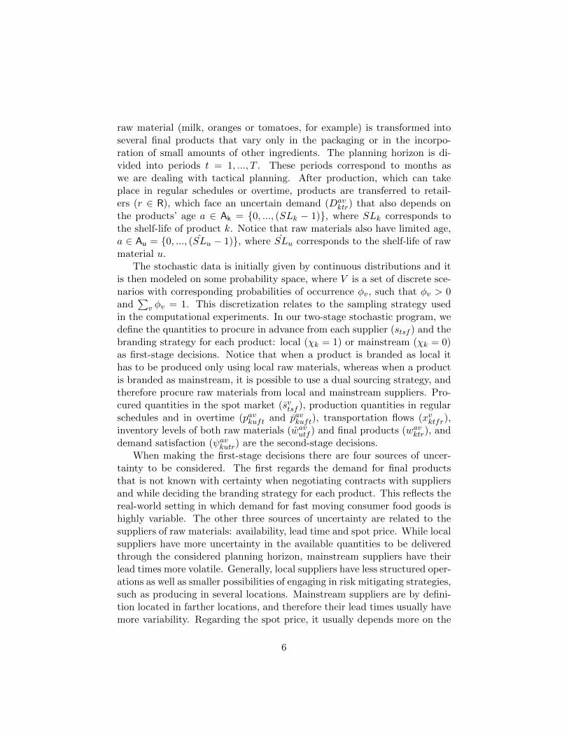
raw material (milk, oranges or tomatoes, for example) is transformed intoseveral final products that vary only in the packaging or in the incorpo-ration of small amounts of other ingredients. The planning horizon is di-vided into periods t = 1, ..., T . These periods correspond to months aswe are dealing with tactical planning. After production, which can takeplace in regular schedules or overtime, products are transferred to retail-ers (r ∈ R), which face an uncertain demand (Dav

ktr) that also depends onthe products’ age a ∈ Ak = 0, ..., (SLk − 1), where SLk corresponds tothe shelf-life of product k. Notice that raw materials also have limited age,a ∈ Au = 0, ..., (SLu − 1), where SLu corresponds to the shelf-life of rawmaterial u.

The stochastic data is initially given by continuous distributions and itis then modeled on some probability space, where V is a set of discrete sce-narios with corresponding probabilities of occurrence φv, such that φv > 0and

∑v φv = 1. This discretization relates to the sampling strategy used

in the computational experiments. In our two-stage stochastic program, wedefine the quantities to procure in advance from each supplier (stsf ) and thebranding strategy for each product: local (χk = 1) or mainstream (χk = 0)as first-stage decisions. Notice that when a product is branded as local ithas to be produced only using local raw materials, whereas when a productis branded as mainstream, it is possible to use a dual sourcing strategy, andtherefore procure raw materials from local and mainstream suppliers. Pro-cured quantities in the spot market (svtsf ), production quantities in regularschedules and in overtime (pavkuft and pavkuft), transportation flows (xvktfr),inventory levels of both raw materials (wavutf ) and final products (wavktr), anddemand satisfaction (ψavkutr) are the second-stage decisions.

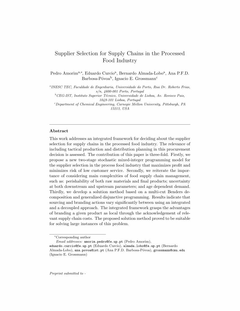
When making the first-stage decisions there are four sources of uncer-tainty to be considered. The first regards the demand for final productsthat is not known with certainty when negotiating contracts with suppliersand while deciding the branding strategy for each product. This reflects thereal-world setting in which demand for fast moving consumer food goods ishighly variable. The other three sources of uncertainty are related to thesuppliers of raw materials: availability, lead time and spot price. While localsuppliers have more uncertainty in the available quantities to be deliveredthrough the considered planning horizon, mainstream suppliers have theirlead times more volatile. Generally, local suppliers have less structured oper-ations as well as smaller possibilities of engaging in risk mitigating strategies,such as producing in several locations. Mainstream suppliers are by defini-tion located in farther locations, and therefore their lead times usually havemore variability. Regarding the spot price, it usually depends more on the

6

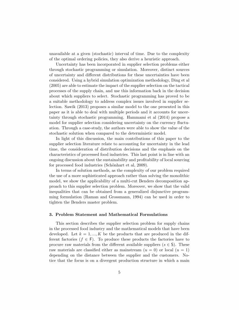
negotiation undertaken and on the yields of that period than on the type ofsupplier. Negotiating in the spot market has a critical component of priceuncertainty that is reflected in our model. Figure 1 illustrates the generalproblem framework and clarifies the connection between the formulationstages and the supply chain processes.

Supplier Selection Model for Supply Chains in the Processed Food Industry

Supply Chain Scope in the Processed Food Industry

Production Planning

Distribution Planning

Factories

Local Suppliers

Mainstream Suppliers

Warehouses/Retailers

Perishability

Infl

uen

ce

1st Stage Decisions 2nd Stage Decisions

Product Branding

Dem

and

Age

Mainstream

Local

Purchases in Advance

Spot Purchases

Pri

ce

Branding

Local

Supplier Uncertainties Demand Uncertainty

Figure 1: Overview of the scope of this research.

Consider the following indices, parameters, and decision variables thatare used in the stochastic formulation.

Indices and Setsk ∈ K final productsu ∈ U supplier / raw material classification: 0 for mainstream, 1 for

locals ∈ S suppliersf ∈ F factoriesr ∈ R retailerst ∈ T periodsa ∈ A ages (in periods)v ∈ V scenariosSu set of suppliers that supply raw material of type uAk set of ages that product k may haveAu set of ages that raw-material u may have

7

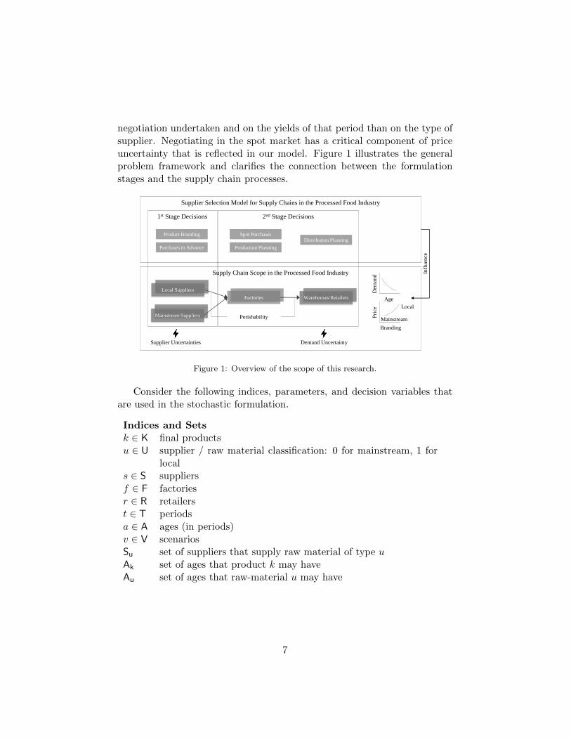
Deterministic ParametersSPs unit purchasing cost of raw material when bought in advance

at supplier s

TCsf ( ˆTCfr) transportation cost from supplier s (factory f) to factory f(retailer r)

SLk(SLu) shelf-life duration of product k (raw material u) right afterbeing produced (time)

HCk( ˆHCu) holding cost for product k (raw material u)PCkf (PCkf ) normal (extra) production cost for product k when produced

in factory fLPku list price for product k when branded as product of type uEkf capacity consumption (time) needed to produce one unit of

product k in factory fCPtf (CP tf ) normal (extra) capacity of factory f available in period t

Stochastic ParametersDavktr demand at retailer r for product k with age a in period t in scenario

vLT vts lead time offset of a shipment due to arrive in period t from supplier

s in scenario vSP

vs unit purchasing cost of raw material when bought in a spot deal from

supplier s in scenario vAQvts availability of raw material at supplier s for supplying in period t in

scenario vφv probability of occurrence of scenario v

First-Stage Decision Variablesstsf quantity of raw material procured in advance from supplier s in

period t for supplying factory fχk equals 1, if product k is produced using only local raw materials

(0 otherwise)η value-at-risk of the customer service

8

Second-Stage Decision Variablesτavtsf auxiliary variable that quantifies the amount of raw material

procured in advance from supplier s that arrives in period twith age a for supplying factory f in scenario v

svtsf quantity of raw material procured with a spot deal fromsupplier s in period t for supplying factory f in scenario v

pavkutf (pavkutf ) regular (overtime) produced quantity of product k in factoryf using raw-materials of type u with age a in period t andscenario v

xvktfr transported quantity of product k from factory f to retailerr in period t and scenario v

wavktr(wavutf ) initial inventory of product k (raw material u) with age

a in period t in scenario v at retailer r (factory f), a =0, ...,minSLk, t− 1(a = 0, ...,minSLu, t− 1)

ψavkutr fraction of the demand for product k produced with suppli-ers of type u delivered with age a in period t in scenario vfrom retailer r, a = 0, ...,minSLk, t− 1

δv auxiliary variable for calculating the conditional value-at-risk of the customer service

3.1. Mixed-integer Linear Programming Formulation

The mixed-integer linear programming formulation of the problem isdescribed next. The constraints that this problem is subject to are organizedaround the respective supply chain echelon.

3.1.1. Objective Function

The first part of objective function (1) maximizes the profit of the pro-ducer over the tactical planning horizon. Expected revenue, which dependson the products’ branding is subtracted by supply chain related costs: pur-chasing costs of raw materials, both when bought in advance and or in thespot market, holding costs for raw materials and final products, transporta-tion costs between the supply chain nodes, and normal and extra productioncosts. The second part the objective function maximizes the (1 − α) · 100scenarios that yield the lowest customer service. This is an adaptation ofthe Conditional Value-at-Risk (Rockafellar and Uryasev, 2000, 2002) focus-ing on the customer service. Similar concepts, such as the supply-at-risk(SaR) were developed in a similar context Hong and Lee (2013). The mainadvantages of these type of metrics is that they are less influenced by veryunlikely uncertain scenarios that could steer the whole solution structure to

9

a very conservative behavior. The risk-aversion of the objective function iscontrolled by weight parameter γ.

max∑v

φv[∑

k,u,t,r,a

LPku ·D0vktr · ψavkutr −

∑k,t,r,a<SLk

HCk · wavktr −∑k,t,f,r

ˆTCfr · xvktfr

−∑

k,u,t,f,a

(PCkf · pavkutf + PCkf · pavkutf )−∑

u,t,f,a<SLu

HCu · wavutf

−∑s,f

(SPvs + TCsf ) · svtsf −

∑t,s,f,a

(SPs + TCsf ) · τavtsf ] + γ · (η − 1

1− α∑v

φv · δv) (1)

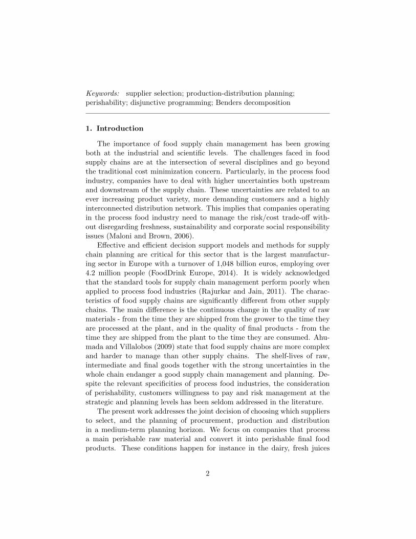
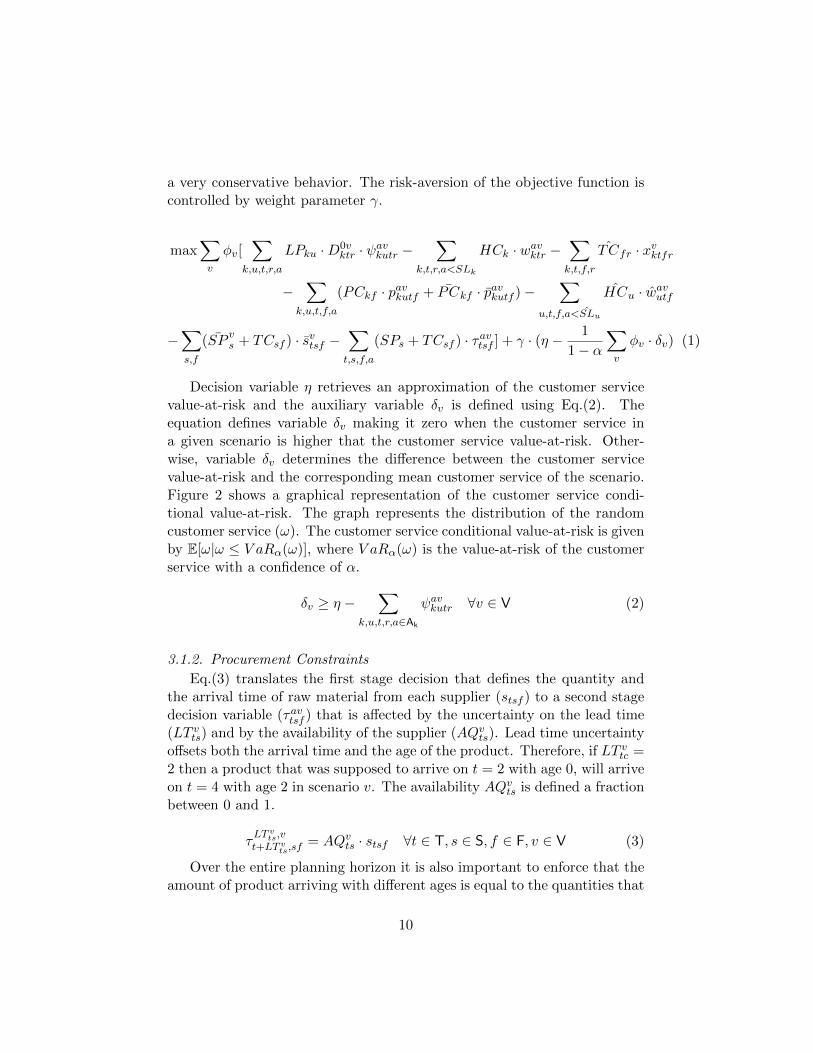
Decision variable η retrieves an approximation of the customer servicevalue-at-risk and the auxiliary variable δv is defined using Eq.(2). Theequation defines variable δv making it zero when the customer service ina given scenario is higher that the customer service value-at-risk. Other-wise, variable δv determines the difference between the customer servicevalue-at-risk and the corresponding mean customer service of the scenario.Figure 2 shows a graphical representation of the customer service condi-tional value-at-risk. The graph represents the distribution of the randomcustomer service (ω). The customer service conditional value-at-risk is givenby E[ω|ω ≤ V aRα(ω)], where V aRα(ω) is the value-at-risk of the customerservice with a confidence of α.

δv ≥ η −∑

k,u,t,r,a∈Ak

ψavkutr ∀v ∈ V (2)

3.1.2. Procurement Constraints

Eq.(3) translates the first stage decision that defines the quantity andthe arrival time of raw material from each supplier (stsf ) to a second stagedecision variable (τavtsf ) that is affected by the uncertainty on the lead time(LT vts) and by the availability of the supplier (AQvts). Lead time uncertaintyoffsets both the arrival time and the age of the product. Therefore, if LT vtc =2 then a product that was supposed to arrive on t = 2 with age 0, will arriveon t = 4 with age 2 in scenario v. The availability AQvts is defined a fractionbetween 0 and 1.

τLT v

ts,vt+LT v

ts,sf= AQvts · stsf ∀t ∈ T, s ∈ S, f ∈ F, v ∈ V (3)

Over the entire planning horizon it is also important to enforce that theamount of product arriving with different ages is equal to the quantities that

10

Fre

quen

cy

Customer

Service (𝜓)

Customer

Service VaR

VaR

Deviation

Min Customer

Service

Customer

Service cVaR

cVaR

Deviation

Probalility 1-α

Figure 2: Graphical representation of the customer service conditional value-at-risk(adapted from Sarykalin et al (2008)).

the producer has ordered discounted by the availability and arrivals outsidethe planning horizon (4).∑

t,a∈Au

τavtsf =∑t

AQvts · stsf ∀s ∈ S, f ∈ F, v ∈ V (4)

Eq.(5) indicates that the inventory amount of raw material available toprocess at factory f with age 0 is equivalent to the amount bought in thespot market and bought in advance when there were no delivery delays.∑

s∈Su

(τ0vtsf + svtsf ) = w0vutf ∀u ∈ U, t ∈ T, f ∈ F, v ∈ V (5)

3.1.3. Production Constraints

Eq.(6) acts as an inventory balance constraint for the stock of the raw-materials. It also updates the age of the raw material stock and takes intoaccount the raw materials arriving with older ages (larger than 0). Noticethat the domain of the inventory variables is constrained in its definition inthe beginning of Section 3.

wavutf = wa−1,vu,t−1,f +∑s∈Su

τavtsf −∑k

(pa−1,vku,t−1,f + pa−1,vku,t−1,f )

∀u ∈ U, t ∈ 2, ..., T + 1, f ∈ F, a ∈ Au : a ≥ 1, v ∈ V (6)

11

Eq.(7) forces the utilization of local raw material in case the product isbranded as local.

pavk0tf + pavk0tf ≤M(1− χk) ∀k ∈ K, t ∈ T, f ∈ F, a ∈ Au : u = 0, v ∈ V (7)

Eqs.(8)-(9) limit both normal and extra production to the available fac-tory capacity, respectively.∑

k,u,a∈Au

Ekfpavkutf ≤ CPft ∀t ∈ T, f ∈ F, v ∈ V (8)

∑k,u,a∈Au

Ekf pavkutf ≤ CP ft ∀t ∈ T, f ∈ F, v ∈ V (9)

3.1.4. Distribution Constraints

Eq.(10) forces all production made in the different factories to flow toretailers within the same planning period.∑

u,a∈Au

pavkutf =∑r

xvktfr ∀k ∈ K, t ∈ T, f ∈ F, v ∈ V (10)

The amount of final products entering each retailer corresponds to theinventory available to satisfy demand with age 0 (11). Therefore, notice thatafter processing the raw-materials, the age of the final products is alwaysset to 0. ∑

f

xvktfr = w0vktr ∀k ∈ K, t ∈ T, r ∈ R, v ∈ V (11)

3.1.5. Demand Fulfillment Constraints

Eqs.(12)-(13) link the choice on the product branding as local (χk =1, u = 1) or mainstream (χk = 0, u = 0) to the type of demand fulfilled thatwill determine the list price that the customer pays. These constraints definethe revenue of the solution with the first term of the objective function (1).

ψavk0tr ≤ 1− χk ∀k ∈ K, t ∈ T, r ∈ R, a ∈ Ak, v ∈ V (12)

ψavk1tr ≤ χk ∀k ∈ K, t ∈ T, r ∈ R, a ∈ Ak, v ∈ V (13)

Eq.(14) is another inventory balance constraint, but this time in theretailers’ premises for final products. This constraint updates the age offinal products’ inventory throughout the planning periods.

12

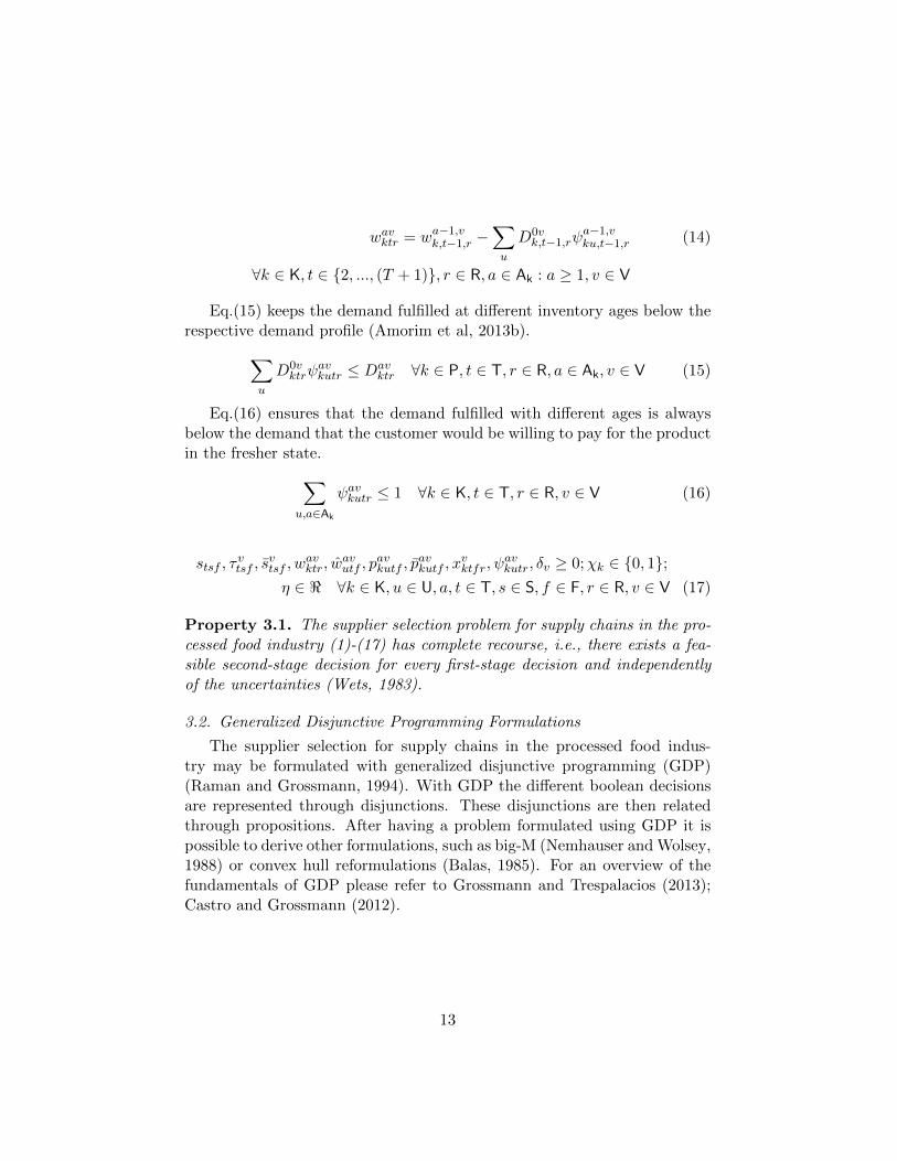
wavktr = wa−1,vk,t−1,r −∑u

D0vk,t−1,rψ

a−1,vku,t−1,r (14)

∀k ∈ K, t ∈ 2, ..., (T + 1), r ∈ R, a ∈ Ak : a ≥ 1, v ∈ V

Eq.(15) keeps the demand fulfilled at different inventory ages below therespective demand profile (Amorim et al, 2013b).∑

u

D0vktrψ

avkutr ≤ Dav

ktr ∀k ∈ P, t ∈ T, r ∈ R, a ∈ Ak, v ∈ V (15)

Eq.(16) ensures that the demand fulfilled with different ages is alwaysbelow the demand that the customer would be willing to pay for the productin the fresher state.∑

u,a∈Ak

ψavkutr ≤ 1 ∀k ∈ K, t ∈ T, r ∈ R, v ∈ V (16)

stsf , τvtsf , s

vtsf , w

avktr, w

avutf , p

avkutf , p

avkutf , x

vktfr, ψ

avkutr, δv ≥ 0;χk ∈ 0, 1;

η ∈ < ∀k ∈ K, u ∈ U, a, t ∈ T, s ∈ S, f ∈ F, r ∈ R, v ∈ V (17)

Property 3.1. The supplier selection problem for supply chains in the pro-cessed food industry (1)-(17) has complete recourse, i.e., there exists a fea-sible second-stage decision for every first-stage decision and independentlyof the uncertainties (Wets, 1983).

3.2. Generalized Disjunctive Programming Formulations

The supplier selection for supply chains in the processed food indus-try may be formulated with generalized disjunctive programming (GDP)(Raman and Grossmann, 1994). With GDP the different boolean decisionsare represented through disjunctions. These disjunctions are then relatedthrough propositions. After having a problem formulated using GDP it ispossible to derive other formulations, such as big-M (Nemhauser and Wolsey,1988) or convex hull reformulations (Balas, 1985). For an overview of thefundamentals of GDP please refer to Grossmann and Trespalacios (2013);Castro and Grossmann (2012).

13

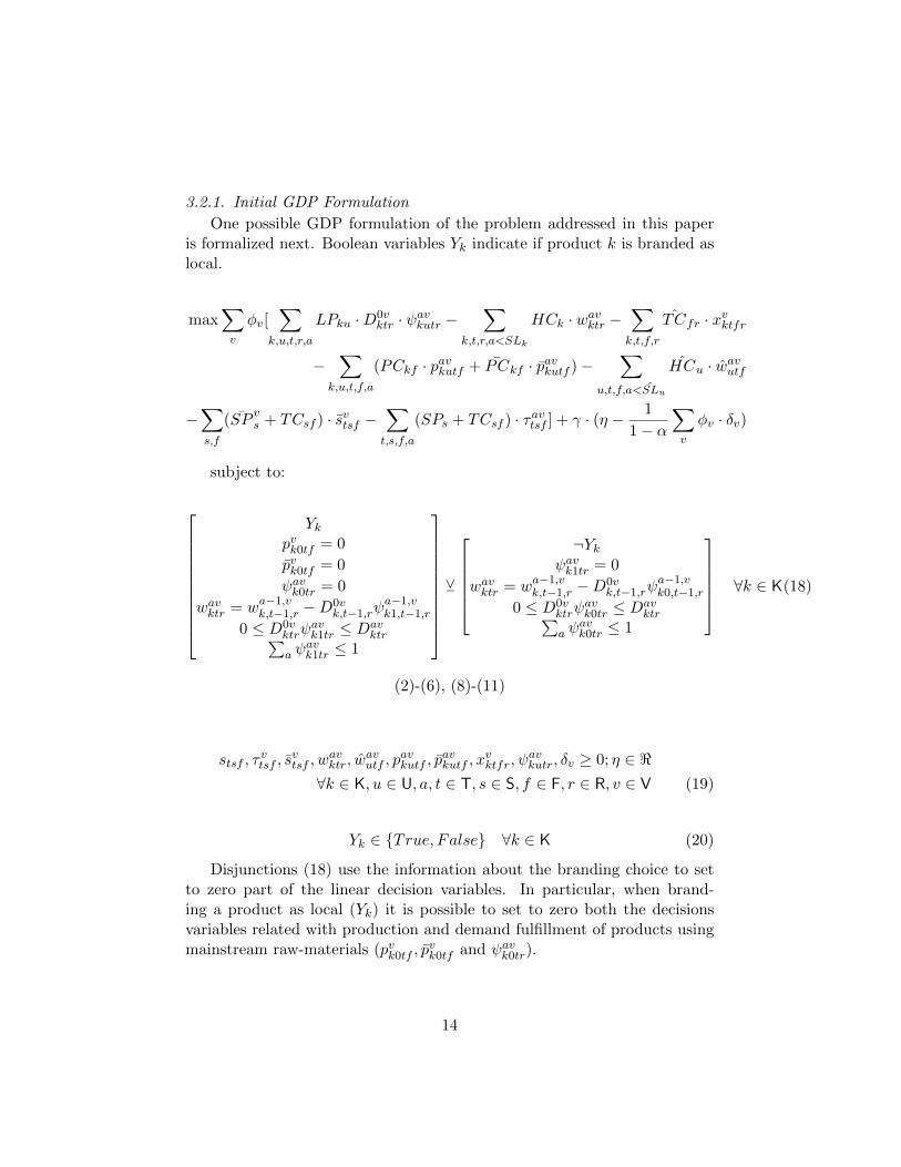
3.2.1. Initial GDP Formulation

One possible GDP formulation of the problem addressed in this paperis formalized next. Boolean variables Yk indicate if product k is branded aslocal.

max∑v

φv[∑

k,u,t,r,a


∑k,t,r,a<SLk


ˆTCfr · xvktfr

−∑

k,u,t,f,a


u,t,f,a<SLu

HCu · wavutf

−∑s,f


∑t,s,f,a


1− α∑v

φv · δv)

subject to:

Ykpvk0tf = 0

pvk0tf = 0

ψavk0tr = 0

wavktr = wa−1,vk,t−1,r −D0vk,t−1,rψ

a−1,vk1,t−1,r

0 ≤ D0vktrψ

avk1tr ≤ Dav

ktr∑a ψ

avk1tr ≤ 1

Y

¬Yk

ψavk1tr = 0

wavktr = wa−1,vk,t−1,r −D0vk,t−1,rψ

a−1,vk0,t−1,r

0 ≤ D0vktrψ

avk0tr ≤ Dav

ktr∑a ψ

avk0tr ≤ 1

∀k ∈ K(18)

(2)-(6), (8)-(11)

stsf , τvtsf , s

vtsf , w

avktr, w

avutf , p

avkutf , p

avkutf , x

vktfr, ψ

avkutr, δv ≥ 0; η ∈ <

∀k ∈ K, u ∈ U, a, t ∈ T, s ∈ S, f ∈ F, r ∈ R, v ∈ V (19)

Yk ∈ True, False ∀k ∈ K (20)

Disjunctions (18) use the information about the branding choice to setto zero part of the linear decision variables. In particular, when brand-ing a product as local (Yk) it is possible to set to zero both the decisionsvariables related with production and demand fulfillment of products usingmainstream raw-materials (pvk0tf , p

vk0tf and ψavk0tr).

14

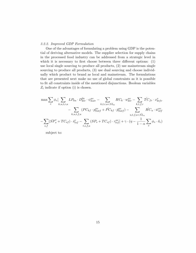
3.2.2. Improved GDP Formulation

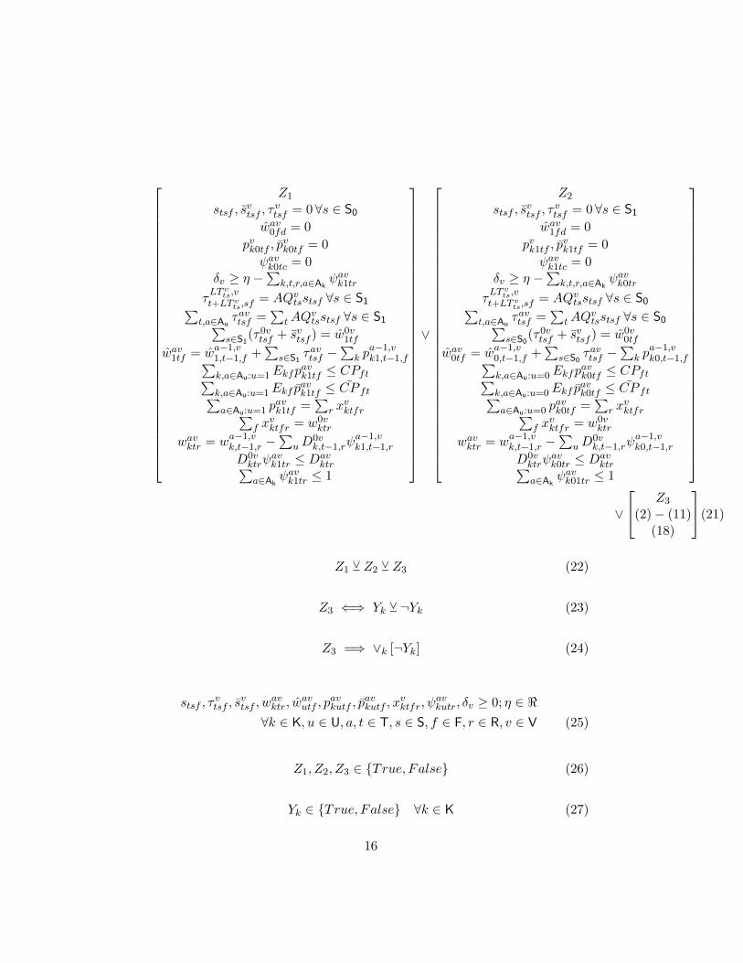
One of the advantages of formulating a problem using GDP is the poten-tial of deriving alternative models. The supplier selection for supply chainsin the processed food industry can be addressed from a strategic level inwhich it is necessary to first choose between three different options: (1)use local single sourcing to produce all products, (2) use mainstream singlesourcing to produce all products, (3) use dual sourcing and choose individ-ually which product to brand as local and mainstream. The formulationsthat are presented next make no use of global constraints as it is possibleto fit all constraints inside of the mentioned disjunctions. Boolean variablesZi indicate if option (i) is chosen.

max∑v

φv[∑

k,u,t,r,a


∑k,t,r,a<SLk


ˆTCfr · xvktfr

−∑

k,u,t,f,a


u,t,f,a<SLu

HCu · wavutf

−∑s,f


∑t,s,f,a


1− α∑v

φv · δv)

subject to:

15

Z1

stsf , svtsf , τ

vtsf = 0∀s ∈ S0

wav0fd = 0

pvk0tf , pvk0tf = 0

ψavk0tc = 0δv ≥ η −

∑k,t,r,a∈Ak

ψavk1trτLT v

ts,vt+LT v

ts,sf= AQvtsstsf ∀s ∈ S1∑

t,a∈Auτavtsf =

∑tAQ

vtsstsf ∀s ∈ S1∑

s∈S1(τ0vtsf + svtsf ) = w0v

1tf

wav1tf = wa−1,v1,t−1,f +∑

s∈S1 τavtsf −

∑k p

a−1,vk1,t−1,f∑

k,a∈Au:u=1Ekfpavk1tf ≤ CPft∑

k,a∈Au:u=1Ekf pavk1tf ≤ CP ft∑

a∈Au:u=1 pavk1tf =

∑r x

vktfr∑

f xvktfr = w0v

ktr

wavktr = wa−1,vk,t−1,r −∑

uD0vk,t−1,rψ

a−1,vk1,t−1,r

D0vktrψ

avk1tr ≤ Dav

ktr∑a∈Ak

ψavk1tr ≤ 1

∨

Z2

stsf , svtsf , τ

vtsf = 0∀s ∈ S1

wav1fd = 0

pvk1tf , pvk1tf = 0

ψavk1tc = 0δv ≥ η −

∑k,t,r,a∈Ak

ψavk0trτLT v

ts,vt+LT v

ts,sf= AQvtsstsf ∀s ∈ S0∑

t,a∈Auτavtsf =

∑tAQ

vtsstsf ∀s ∈ S0∑

s∈S0(τ0vtsf + svtsf ) = w0v

0tf

wav0tf = wa−1,v0,t−1,f +∑

s∈S0 τavtsf −

∑k p

a−1,vk0,t−1,f∑

k,a∈Au:u=0Ekfpavk0tf ≤ CPft∑

k,a∈Au:u=0Ekf pavk0tf ≤ CP ft∑

a∈Au:u=0 pavk0tf =

∑r x

vktfr∑

f xvktfr = w0v

ktr

wavktr = wa−1,vk,t−1,r −∑

uD0vk,t−1,rψ

a−1,vk0,t−1,r

D0vktrψ

avk0tr ≤ Dav

ktr∑a∈Ak

ψavk01tr ≤ 1

∨

Z3

(2)− (11)(18)

(21)

Z1 Y Z2 Y Z3 (22)

Z3 ⇐⇒ Yk Y ¬Yk (23)

Z3 =⇒ ∨k [¬Yk] (24)

stsf , τvtsf , s

vtsf , w

avktr, w

avutf , p

avkutf , p

avkutf , x

vktfr, ψ

avkutr, δv ≥ 0; η ∈ <

∀k ∈ K, u ∈ U, a, t ∈ T, s ∈ S, f ∈ F, r ∈ R, v ∈ V (25)

Z1, Z2, Z3 ∈ True, False (26)

Yk ∈ True, False ∀k ∈ K (27)

16

Disjunctions (21) use the information about the sourcing strategy choiceto narrow the search space. The first and the second disjunctions (Z1 andZ2) set to zero all variables related to mainstream sourcing / branding andto local sourcing / branding, respectively. The third disjunction (Z3) has aembedded disjunction similar to the one presented in the previous section(cf. Section 3.2.1). Logic proposition (22) forces the choice of one of thesourcing strategies. Logic proposition (23) states that if a dual sourcingstrategy is chosen then it is necessary to decide for each product the branding(mainstream or local). Finally, logic proposition (24) ensures that whenchoosing a dual sourcing strategy there exists at least one product that isnot branded as local.

The use of GDP modeling in this context will be clearer in Section 5.1where the related convex hull reformulation is used.

4. Illustrative Example

In this section we explore with an illustrative example the importanceof considering uncertainty and the impact of the integrated approach in thesupplier selection for supply chains in the processed food industry.

4.1. Instances Generation

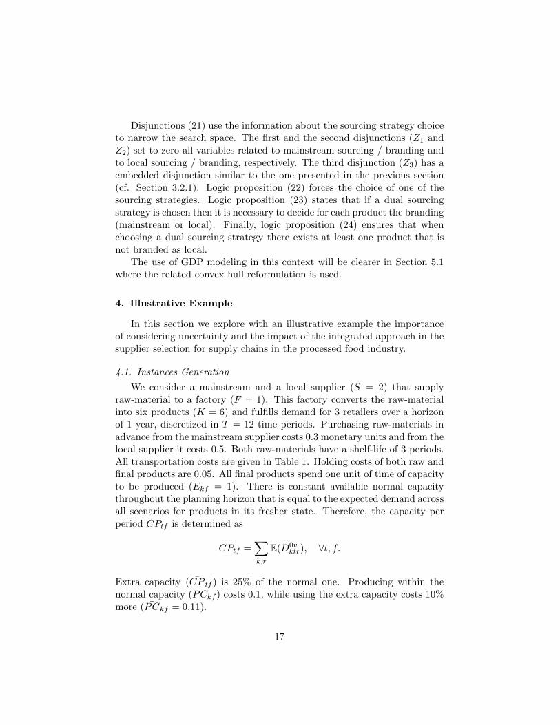
We consider a mainstream and a local supplier (S = 2) that supplyraw-material to a factory (F = 1). This factory converts the raw-materialinto six products (K = 6) and fulfills demand for 3 retailers over a horizonof 1 year, discretized in T = 12 time periods. Purchasing raw-materials inadvance from the mainstream supplier costs 0.3 monetary units and from thelocal supplier it costs 0.5. Both raw-materials have a shelf-life of 3 periods.All transportation costs are given in Table 1. Holding costs of both raw andfinal products are 0.05. All final products spend one unit of time of capacityto be produced (Ekf = 1). There is constant available normal capacitythroughout the planning horizon that is equal to the expected demand acrossall scenarios for products in its fresher state. Therefore, the capacity perperiod CPtf is determined as

CPtf =∑k,r

E(D0vktr), ∀t, f.

Extra capacity (CP tf ) is 25% of the normal one. Producing within thenormal capacity (PCkf ) costs 0.1, while using the extra capacity costs 10%more (PCkf = 0.11).

17

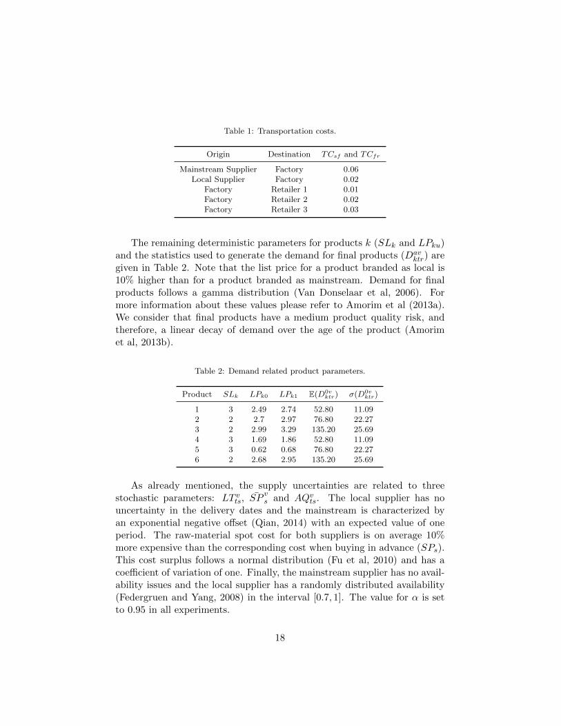
Table 1: Transportation costs.

Origin Destination TCsf and TCfr

Mainstream Supplier Factory 0.06Local Supplier Factory 0.02

Factory Retailer 1 0.01Factory Retailer 2 0.02Factory Retailer 3 0.03

The remaining deterministic parameters for products k (SLk and LPku)and the statistics used to generate the demand for final products (Dav

ktr) aregiven in Table 2. Note that the list price for a product branded as local is10% higher than for a product branded as mainstream. Demand for finalproducts follows a gamma distribution (Van Donselaar et al, 2006). Formore information about these values please refer to Amorim et al (2013a).We consider that final products have a medium product quality risk, andtherefore, a linear decay of demand over the age of the product (Amorimet al, 2013b).

Table 2: Demand related product parameters.

Product SLk LPk0 LPk1 E(D0vktr) σ(D0v

ktr)

1 3 2.49 2.74 52.80 11.092 2 2.7 2.97 76.80 22.273 2 2.99 3.29 135.20 25.694 3 1.69 1.86 52.80 11.095 3 0.62 0.68 76.80 22.276 2 2.68 2.95 135.20 25.69

As already mentioned, the supply uncertainties are related to threestochastic parameters: LT vts, SP

vs and AQvts. The local supplier has no

uncertainty in the delivery dates and the mainstream is characterized byan exponential negative offset (Qian, 2014) with an expected value of oneperiod. The raw-material spot cost for both suppliers is on average 10%more expensive than the corresponding cost when buying in advance (SPs).This cost surplus follows a normal distribution (Fu et al, 2010) and has acoefficient of variation of one. Finally, the mainstream supplier has no avail-ability issues and the local supplier has a randomly distributed availability(Federgruen and Yang, 2008) in the interval [0.7, 1]. The value for α is setto 0.95 in all experiments.

18

4.2. Importance of Uncertainty

To measure the importance of uncertainty we use the Expected Valueof Perfect Information (EVPI) and the Value of Stochastic Solution (VSS).These two metrics are often used to evaluate the importance of using stochas-tic solutions over deterministic approximations.

Let RP be the optimal value of solving the two-stage stochastic program-ming problem (1)-(17), and consider WSv the optimal value of solving thesame problem only for scenario v ∈ V. Then, the wait-and-see (WS) solu-tion is determined as the expected value of WSv over all scenarios. EVPI isobtained with the difference between WS and the RP:

EVPI = WS− RP. (28)

The EVPI may be seen as the cost of uncertainty or the maximum amountthe decision maker is willing to pay in order to make a decision without un-certainty. Higher EVPIs mean that uncertainty is important to the problem(Wallace and Ziemba, 2005).

Now, let EV be the solution obtained by solving the problem in whichstochastic parameters are replaced by their expected values. The expectedvalue of using the first-stage decisions of EV over all scenarios is denoted asEEV (expected value of using the EV solution). VSS is obtained as follows:

VSS = RP− EEV. (29)

VSS estimates the profit that may be obtained by adopting the stochasticmodel rather than using the approximated mean-value one. Therefore, VSSshows the cost of ignoring the uncertainty in choosing a first-stage decision(Birge and Louveaux, 1997).

In general, there may be cases in which fixing first-stage decision vari-ables may result in unfeasible EEV problems. However, as the supplierselection for supply chains in the processed food industry has complete re-course that is not the case (cf. Property 3.1).

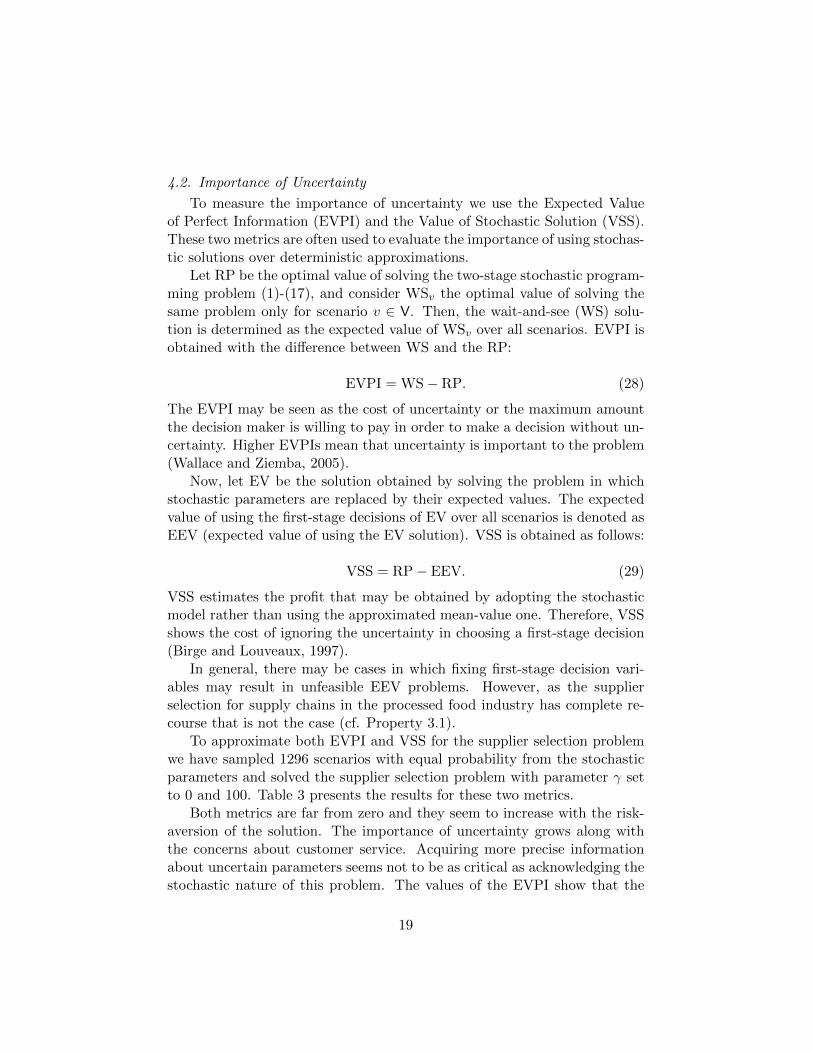
To approximate both EVPI and VSS for the supplier selection problemwe have sampled 1296 scenarios with equal probability from the stochasticparameters and solved the supplier selection problem with parameter γ setto 0 and 100. Table 3 presents the results for these two metrics.

Both metrics are far from zero and they seem to increase with the risk-aversion of the solution. The importance of uncertainty grows along withthe concerns about customer service. Acquiring more precise informationabout uncertain parameters seems not to be as critical as acknowledging thestochastic nature of this problem. The values of the EVPI show that the

19

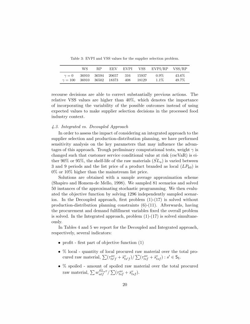
Table 3: EVPI and VSS values for the supplier selection problem.

WS RP EEV EVPI VSS EVPI/RP VSS/RP

γ = 0 36910 36594 20657 316 15937 0.9% 43.6%γ = 100 36910 36502 18373 408 18129 1.1% 49.7%

recourse decisions are able to correct substantially previous actions. Therelative VSS values are higher than 40%, which denotes the importanceof incorporating the variability of the possible outcomes instead of usingexpected values to make supplier selection decisions in the processed foodindustry context.

4.3. Integrated vs. Decoupled Approach

In order to assess the impact of considering an integrated approach to thesupplier selection and production-distribution planning, we have performedsensitivity analysis on the key parameters that may influence the advan-tages of this approach. Trough preliminary computational tests, weight γ ischanged such that customer service conditional value at risk (cscVaR) is ei-ther 90% or 95%, the shelf-life of the raw materials (SLu) is varied between3 and 9 periods and the list price of a product branded as local (LPk0) is0% or 10% higher than the mainstream list price.

Solutions are obtained with a sample average approximation scheme(Shapiro and Homem-de Mello, 1998). We sampled 81 scenarios and solved50 instances of the approximating stochastic programming. We then evalu-ated the objective function by solving 1296 independently sampled scenar-ios. In the Decoupled approach, first problem (1)-(17) is solved withoutproduction-distribution planning constraints (6)-(11). Afterwards, havingthe procurement and demand fulfillment variables fixed the overall problemis solved. In the Integrated approach, problem (1)-(17) is solved simultane-ously.

In Tables 4 and 5 we report for the Decoupled and Integrated approach,respectively, several indicators:

• profit - first part of objective function (1)

• % local - quantity of local procured raw material over the total pro-cured raw material,

∑(τavts′f + svts′f )/

∑(τavtsf + svtsf ) : s′ ∈ S1.

• % spoiled - amount of spoiled raw material over the total procured

raw material,∑wSLuvutf /

∑(τavtsf + svtsf ).

20

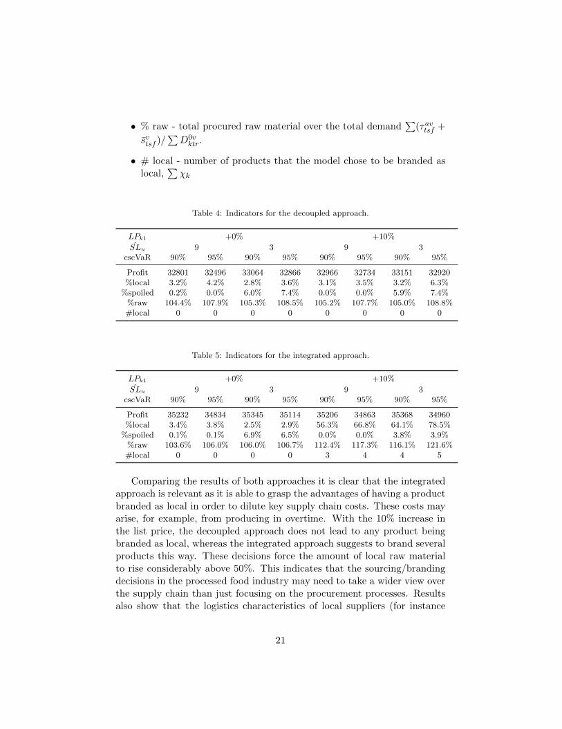
• % raw - total procured raw material over the total demand∑

(τavtsf +

svtsf )/∑D0vktr.

• # local - number of products that the model chose to be branded aslocal,

∑χk

Table 4: Indicators for the decoupled approach.

LPk1 +0% +10%

SLu 9 3 9 3cscVaR 90% 95% 90% 95% 90% 95% 90% 95%

Profit 32801 32496 33064 32866 32966 32734 33151 32920%local 3.2% 4.2% 2.8% 3.6% 3.1% 3.5% 3.2% 6.3%

%spoiled 0.2% 0.0% 6.0% 7.4% 0.0% 0.0% 5.9% 7.4%%raw 104.4% 107.9% 105.3% 108.5% 105.2% 107.7% 105.0% 108.8%#local 0 0 0 0 0 0 0 0

Table 5: Indicators for the integrated approach.

LPk1 +0% +10%

SLu 9 3 9 3cscVaR 90% 95% 90% 95% 90% 95% 90% 95%

Profit 35232 34834 35345 35114 35206 34863 35368 34960%local 3.4% 3.8% 2.5% 2.9% 56.3% 66.8% 64.1% 78.5%

%spoiled 0.1% 0.1% 6.9% 6.5% 0.0% 0.0% 3.8% 3.9%%raw 103.6% 106.0% 106.0% 106.7% 112.4% 117.3% 116.1% 121.6%#local 0 0 0 0 3 4 4 5

Comparing the results of both approaches it is clear that the integratedapproach is relevant as it is able to grasp the advantages of having a productbranded as local in order to dilute key supply chain costs. These costs mayarise, for example, from producing in overtime. With the 10% increase inthe list price, the decoupled approach does not lead to any product beingbranded as local, whereas the integrated approach suggests to brand severalproducts this way. These decisions force the amount of local raw materialto rise considerably above 50%. This indicates that the sourcing/brandingdecisions in the processed food industry may need to take a wider view overthe supply chain than just focusing on the procurement processes. Resultsalso show that the logistics characteristics of local suppliers (for instance

21

smaller and less variable lead time) may not constitute a significant attributeto rise considerably the amount of raw-materials bought from such suppliers.

Taking advantage of the higher customer willingness to pay for localproducts increases profit and lowers the amount of spoiled raw-material.The lower levels of raw-material reaching their shelf-lives is related withthe difference in the lead time uncertainty between mainstream and localsuppliers. On the other hand, both higher service levels and lower shelf-lives of raw materials lead to an increase in the amount of spoiled materialand an increase of the quantities purchased from suppliers in relation tothe actual demand. The quantity of raw-materials procured is also relatedto the amount of local supplies due to the availability uncertainties thatcorresponding suppliers are subject to.

Across all solutions a dual sourcing strategy is used. Regarding the trade-off between profit and cscVaR, it seems that small losses in the average profitmay lead to substantial shift in cscVaR.

5. Multi-Cut Benders Decomposition Algorithm

Even while using a sample average approximation scheme, it is necessaryto solve a large number of two-stage stochastic programs that are not trivialto solve using monolithic models as the ones described in Section 3. In thisSection we discuss a multi-cut Benders decomposition approach that can beembedded in the sample average approximation scheme in a hybrid solutionapproach to solve this supplier selection problem (Santoso et al, 2005).

Benders decomposition (Benders, 1962) is a solution approach that ismore commonly named as L-Shaped method when applied to stochasticprogramming (Van Slyke and Wets, 1969). This solution approach partitionsthe complete formulation into two models. The Benders master problemapproximates the cost of the scenarios in the space of first-stage decisionvariables and the Benders subproblems are obtained from the original one byfixing the first stage variables to the values obtained in the master problem.This solution approach iterates between these two models improving thelower bounds obtained in the master problem (LB) with information comingfrom the upper bounds of the subproblems (UB).

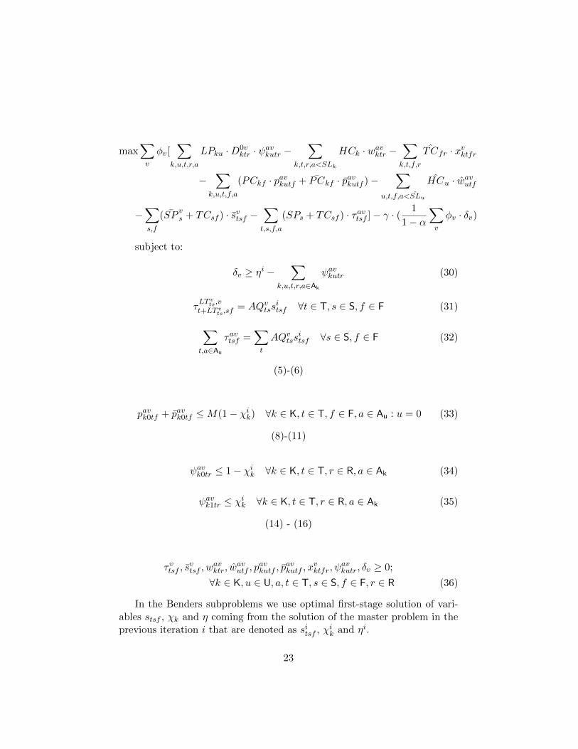
The resulting Benders subproblems (BSP) that may be decomposed foreach scenario v ∈ V are formulated for each iteration i as follows:

22

max∑v

φv[∑

k,u,t,r,a


∑k,t,r,a<SLk


ˆTCfr · xvktfr

−∑

k,u,t,f,a


u,t,f,a<SLu

HCu · wavutf

−∑s,f


∑t,s,f,a

(SPs + TCsf ) · τavtsf ]− γ · ( 1

1− α∑v

φv · δv)

subject to:

δv ≥ ηi −∑

k,u,t,r,a∈Ak

ψavkutr (30)

τLT v

ts,vt+LT v

ts,sf= AQvtss

itsf ∀t ∈ T, s ∈ S, f ∈ F (31)

∑t,a∈Au

τavtsf =∑t

AQvtssitsf ∀s ∈ S, f ∈ F (32)

(5)-(6)

pavk0tf + pavk0tf ≤M(1− χik) ∀k ∈ K, t ∈ T, f ∈ F, a ∈ Au : u = 0 (33)

(8)-(11)

ψavk0tr ≤ 1− χik ∀k ∈ K, t ∈ T, r ∈ R, a ∈ Ak (34)

ψavk1tr ≤ χik ∀k ∈ K, t ∈ T, r ∈ R, a ∈ Ak (35)

(14) - (16)

τvtsf , svtsf , w

avktr, w

avutf , p

avkutf , p

avkutf , x

vktfr, ψ

avkutr, δv ≥ 0;

∀k ∈ K, u ∈ U, a, t ∈ T, s ∈ S, f ∈ F, r ∈ R (36)

In the Benders subproblems we use optimal first-stage solution of vari-ables stsf , χk and η coming from the solution of the master problem in theprevious iteration i that are denoted as sitsf , χik and ηi.

23

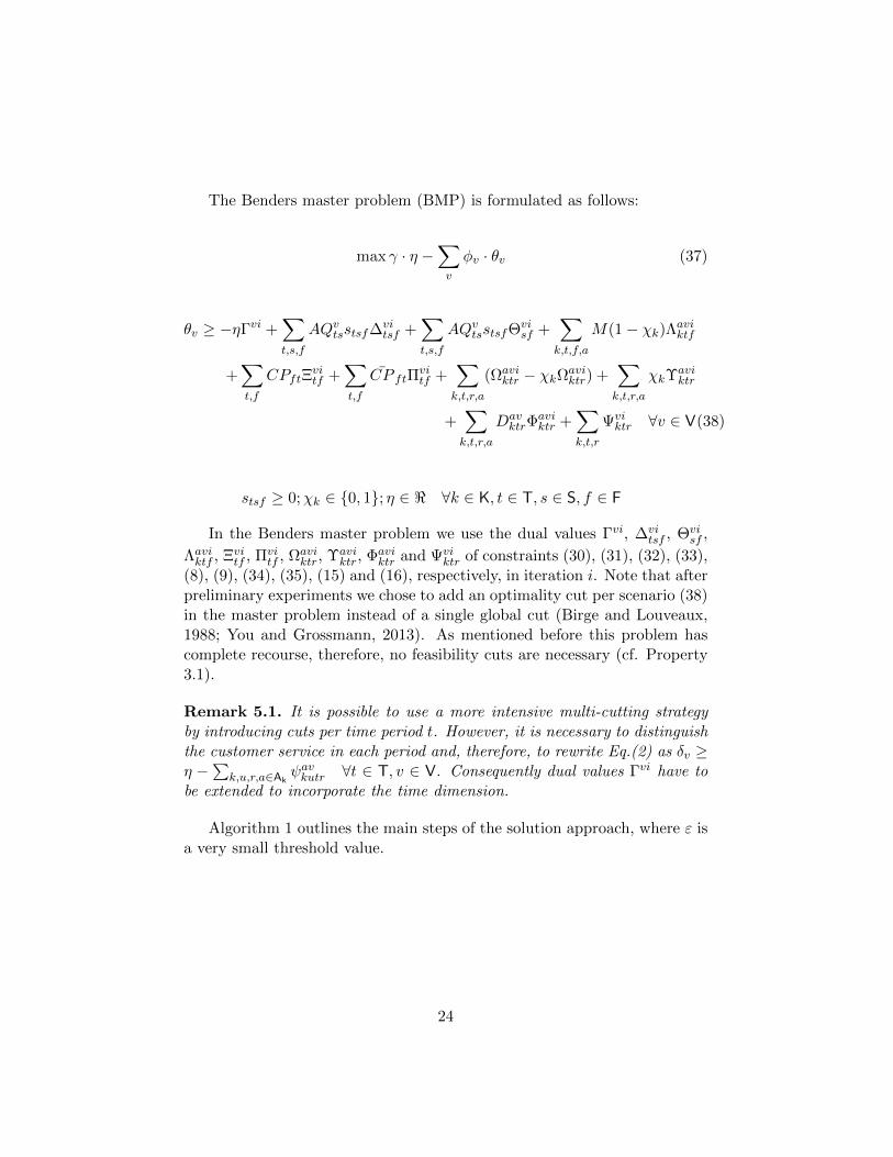
The Benders master problem (BMP) is formulated as follows:

max γ · η −∑v

φv · θv (37)

θv ≥ −ηΓvi +∑t,s,f

AQvtsstsf∆vitsf +

∑t,s,f

AQvtsstsfΘvisf +

∑k,t,f,a

M(1− χk)Λaviktf

+∑t,f

CPftΞvitf +

∑t,f

CP ftΠvitf +

∑k,t,r,a

(Ωaviktr − χkΩavi

ktr) +∑k,t,r,a

χkΥaviktr

+∑k,t,r,a

DavktrΦ

aviktr +

∑k,t,r

Ψviktr ∀v ∈ V(38)

stsf ≥ 0;χk ∈ 0, 1; η ∈ < ∀k ∈ K, t ∈ T, s ∈ S, f ∈ F

In the Benders master problem we use the dual values Γvi, ∆vitsf , Θvi

sf ,

Λaviktf , Ξvitf , Πvitf , Ωavi

ktr, Υaviktr, Φavi

ktr and Ψviktr of constraints (30), (31), (32), (33),

(8), (9), (34), (35), (15) and (16), respectively, in iteration i. Note that afterpreliminary experiments we chose to add an optimality cut per scenario (38)in the master problem instead of a single global cut (Birge and Louveaux,1988; You and Grossmann, 2013). As mentioned before this problem hascomplete recourse, therefore, no feasibility cuts are necessary (cf. Property3.1).

Remark 5.1. It is possible to use a more intensive multi-cutting strategyby introducing cuts per time period t. However, it is necessary to distinguishthe customer service in each period and, therefore, to rewrite Eq.(2) as δv ≥η −

∑k,u,r,a∈Ak

ψavkutr ∀t ∈ T, v ∈ V. Consequently dual values Γvi have tobe extended to incorporate the time dimension.

Algorithm 1 outlines the main steps of the solution approach, where ε isa very small threshold value.

24

Algorithm 1: Outline of Benders solution approach.

initialize s0tsf , χ0k and η0;

set UB =∞ and LB = −∞;while UB − LB > ε do

Solve BSP;Get Second-Stage Variables;Update UB;Get Duals;Add Optimality Cuts to BMP;Get stsf , χk, η;Update LB;Update sitsf , χik and ηi on the BSP;

end

The Benders decomposition algorithm is known to have some conver-gence issues that can be mitigated through acceleration techniques. In theremainder of this section we discuss approaches that can be used to this end.

5.1. Tightening the Benders Master Problem

The resulting BMP from the original formulation (cf. Section 3.1) has noconstraints besides the on-the-fly optimality cuts and the decision variablesdomain constraints. Therefore, before “enough” cuts are added into theBMP the convergence of the solution approach is expected to be ratherslow. The lack of first-stage constraints is related to two characteristicsof this problem. Firstly, the uncertainty of suppliers both in the availablequantity and on the lead time forces a translation of the purchased quantitiesin advance stsf into a second-stage decision variable τavtsf . Secondly, the twomain first-stage decision variables (stsf and χk) are not tightly related dueto the multi-echelon scope of the supplier selection for supply chains in theprocessed food industry, which separates the acquisition of raw-materials ufrom the transformation and selling of final products k.

With the GDP formulation presented in Section 3.2.2 we are able totighten the first-stage decisions by introducing the three disjunctions Zi re-lated with the sourcing strategy. Transforming the GDP formulation intoa mixed-integer programming model by applying classical Boolean algebrarules to convert the logic propositions (Williams, 1999) and reformulatingthe disjunctions using a hull reformulation (Lee and Grossmann, 2000) re-sults in the following first-stage constraints that are added to the BMP.

z1 ≤ χk ∀k ∈ K (39)

25

1− z2 ≥ χk ∀k ∈ K (40)

K − z3 ≥∑k

χk (41)

z1 + z2 + z3 = 1 (42)

stsf = s2tsf + s3tsf ∀t ∈ T, s ∈ S0, f ∈ F (43)

stsf = s1tsf + s3tsf ∀t ∈ T, s ∈ S1, f ∈ F (44)

0 ≤ s1tsf ≤∑t′≥t

(CPft + CP ft)z1 ∀t ∈ T, s ∈ S1, f ∈ F (45)

0 ≤ s2tsf ≤∑t′≥t

(CPft + CP ft)z2 ∀t ∈ T, s ∈ S0, f ∈ F (46)

0 ≤ s3tsf ≤∑t′≥t

(CPft + CP ft)z3 ∀t ∈ T, s ∈ S, f ∈ F (47)

z1, z2, z3 ∈ 0, 1 (48)

Note that χk are the binary variables resulting from transforming Booleanvariables Yk and z1, z2, z3 are the binary variables resulting from transform-ing Boolean variables Z1, Z2, Z3, respectively. Moreover, s1tsf , s

2tsf , s

3tsf are

the disaggregated variables of stsf for each disjunctive term.

5.2. Convex Combinations

The key idea in this acceleration scheme is to consider prior solutionsto the BMP, and then to modify the evaluation of the objective function toalso optimize over best convex combination multipliers (Smith, 2004).

Let sitsf , χik and ηi for i = 1, ..., I be the solutions found after solvingthe BMP over the last I iterations. Parameter I controls the frequency forwhich the modified BSP (mBSP) is solved. In this problem the solutionof the first-stage decision variables stsf , χk and η that was found in theprevious iteration is replaced by the convex combination of these variables

26

over the past I iterations∑

i λisitsf ,

∑i λiχ

ik and

∑i λiη

i, respectively. Theobjective function (30) is modified by adding the following term∑

i

λi · γ · ηi.

Moreover, it is necessary to add the following constraints:

0 ≤ λ ≤ 1 (49)

∑i

λi = 1 (50)

After solving mBSP in a given iteration, Algorithm 1 proceeds by gettingthe dual values of the subproblem constraints and adding the associated cutsto the BMP. Once mBSP is solved in one iteration, BSP is solved for thenext I iterations.

5.3. Solving a Single Benders Master Problem

In the classical Benders solution approach, outlined in Algorithm 1, wealternate between solving a master problem and the subproblems. In thisacceleration scheme we solve a single master problem and generate Benderscuts on the fly as we find feasible master solutions. This general approach isnamed branch-and-check (Thorsteinsson, 2001). This approach can be alsoseen as a branch-and-cut algorithm with the Benders subproblems sourcingthe cuts. In the reminder of the paper we use modern Benders to refer tothis approach.

This approach takes advantage of callback functions in the solver of themaster problem. Its main advantage is that it avoids considerable reworkin the branch-and-bound because we are keeping the same tree throughoutthe iterations of the Benders algorithm. Its main drawback is the harderimplementation procedure.

6. Computational Experiments

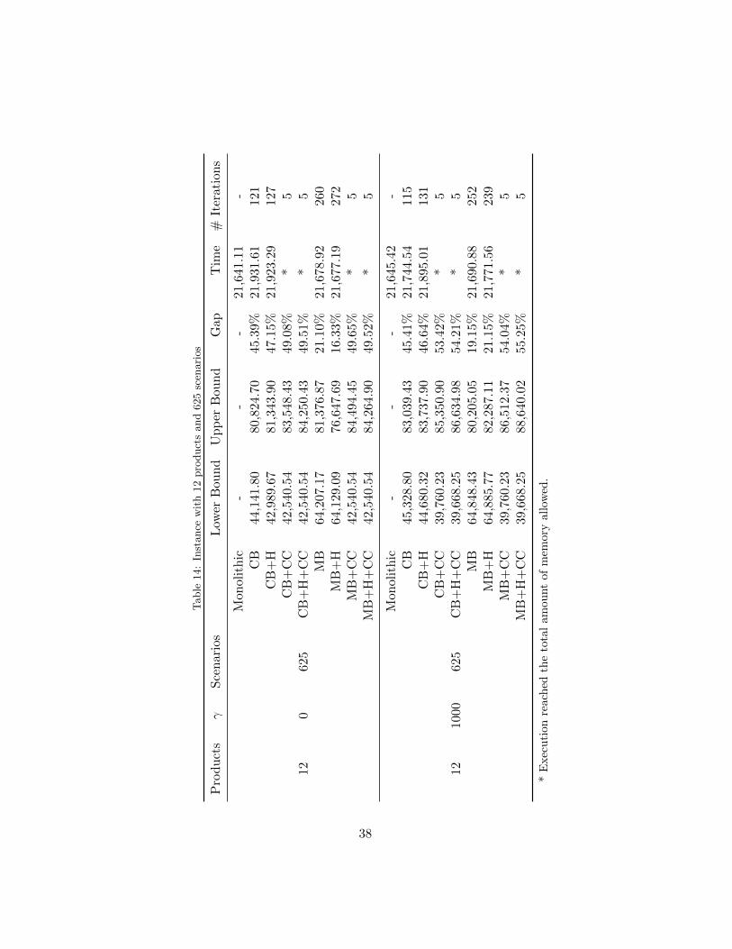
In this section we describe computational experiments using the multi-cut Benders decomposition algorithm presented in Section 5. We sampled81, 256 and 625 scenarios from the instances described in Section 4.1 andsolved for the case in which it is necessary to decide about the supply-ing/branding strategy of 6, 12 and 24 products. Parameter γ was set to 0and to 1000. Therefore, in total we report results for 18 instances. All the

27

programs were implemented in C++ and solved using IBM ILOG CPLEXOptimization Studio 12.4 on an Intel E5-2450 processor under a ScientificLinux 6.5 platform. For instances with 81 scenarios, each run was limitedto 2 cores of the processor and 8GB of RAM. For instances with 12 and 24products under 256 and 625 scenarios the execution was limited to 3 coresand 12GB of RAM.

In order to achieve better computational results, we solved the scenariosubproblems with parallel computing. We grouped the scenarios into sub-problems, in a way that each subproblem has 9 to 50 scenarios, dependingof the number of scenarios in each instance. This method was effective inimproving the computational performance and in reducing the amount ofRAM required.

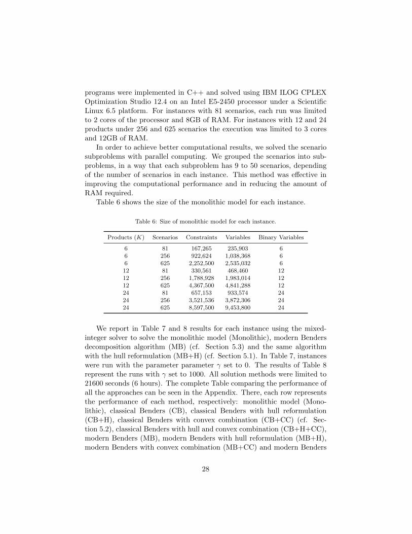
Table 6 shows the size of the monolithic model for each instance.

Table 6: Size of monolithic model for each instance.

Products (K) Scenarios Constraints Variables Binary Variables

6 81 167,265 235,903 66 256 922,624 1,038,368 66 625 2,252,500 2,535,032 612 81 330,561 468,460 1212 256 1,788,928 1,983,014 1212 625 4,367,500 4,841,288 1224 81 657,153 933,574 2424 256 3,521,536 3,872,306 2424 625 8,597,500 9,453,800 24

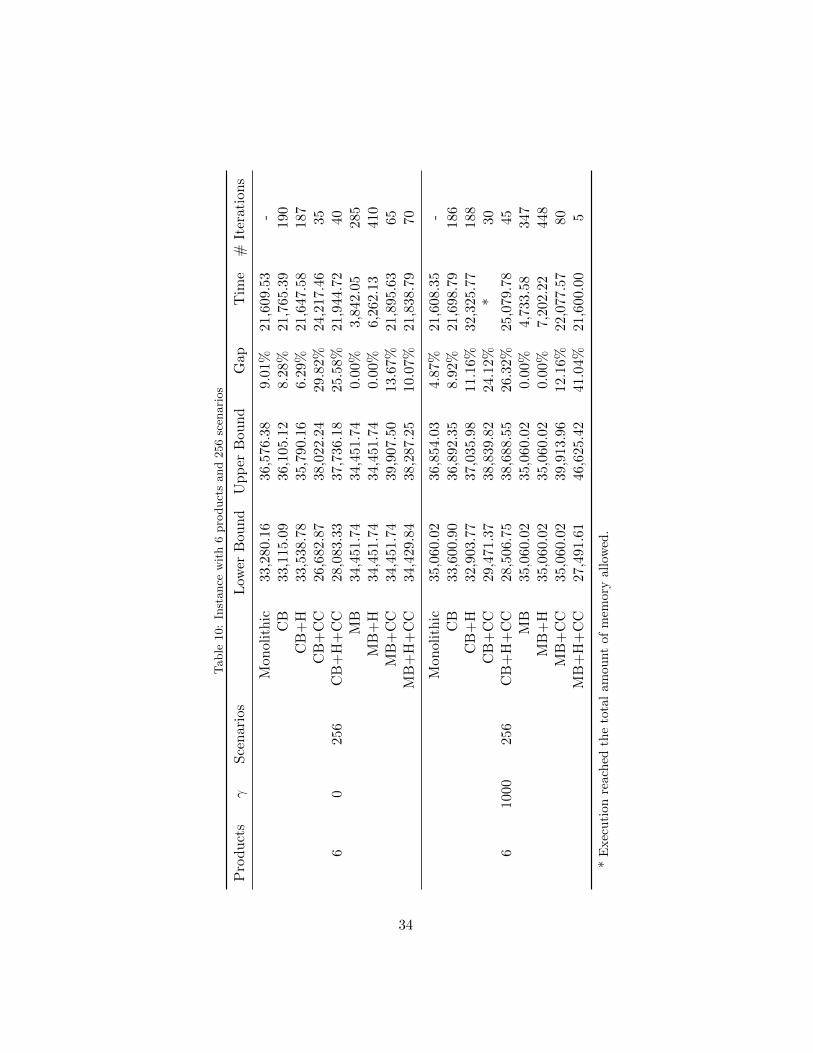
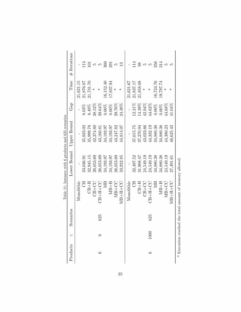
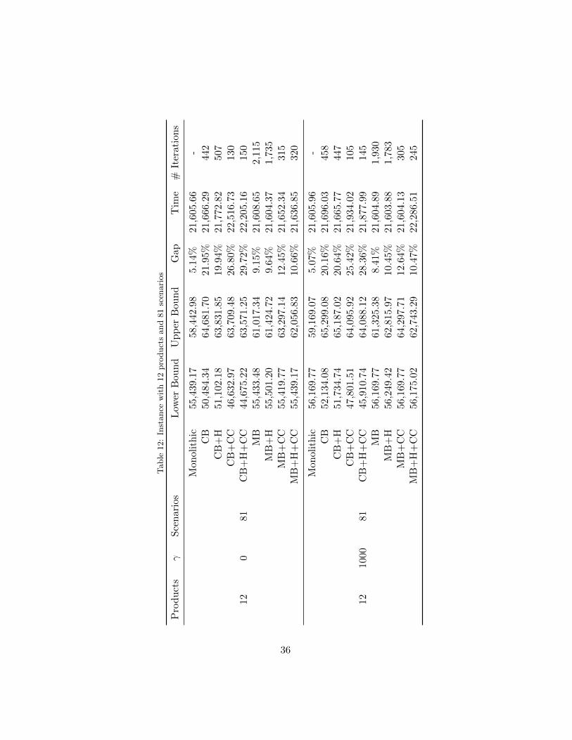
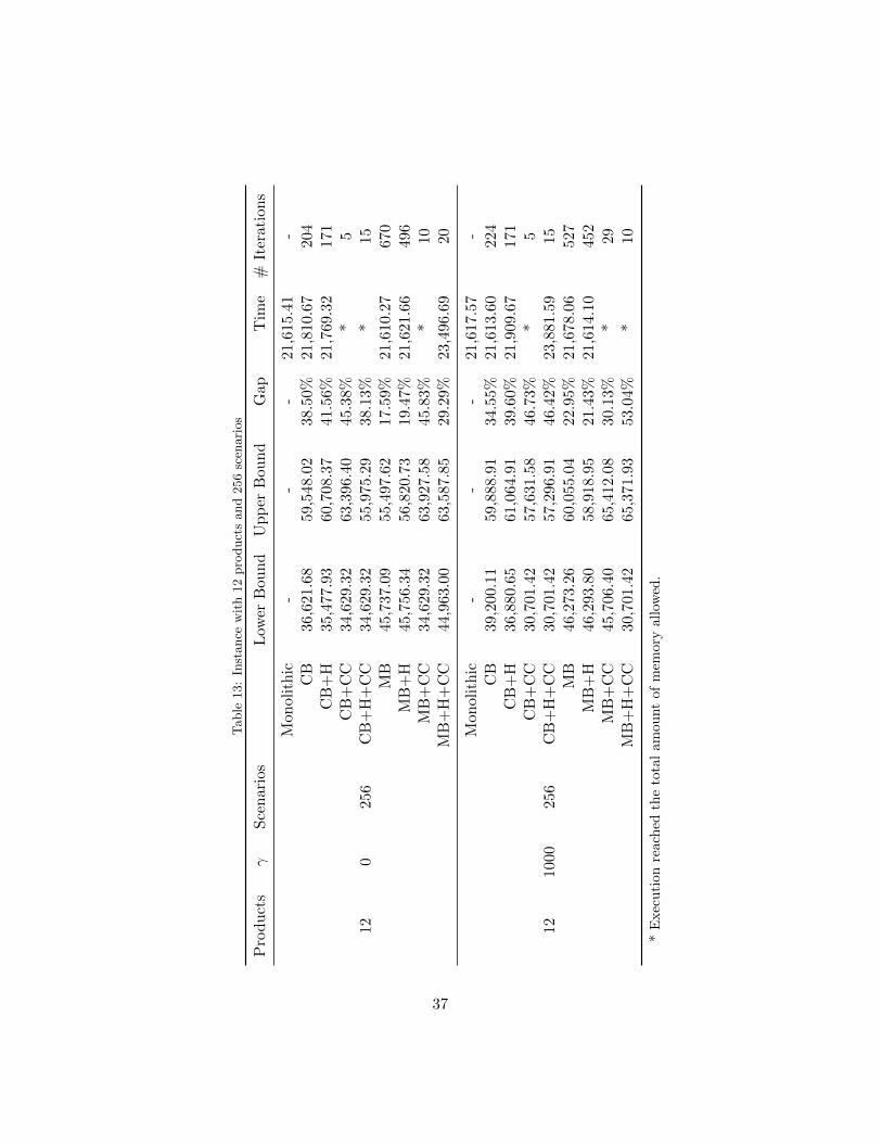
We report in Table 7 and 8 results for each instance using the mixed-integer solver to solve the monolithic model (Monolithic), modern Bendersdecomposition algorithm (MB) (cf. Section 5.3) and the same algorithmwith the hull reformulation (MB+H) (cf. Section 5.1). In Table 7, instanceswere run with the parameter parameter γ set to 0. The results of Table 8represent the runs with γ set to 1000. All solution methods were limited to21600 seconds (6 hours). The complete Table comparing the performance ofall the approaches can be seen in the Appendix. There, each row representsthe performance of each method, respectively: monolithic model (Mono-lithic), classical Benders (CB), classical Benders with hull reformulation(CB+H), classical Benders with convex combination (CB+CC) (cf. Sec-tion 5.2), classical Benders with hull and convex combination (CB+H+CC),modern Benders (MB), modern Benders with hull reformulation (MB+H),modern Benders with convex combination (MB+CC) and modern Benders

28

with hull and convex combination (CB+H+CC).

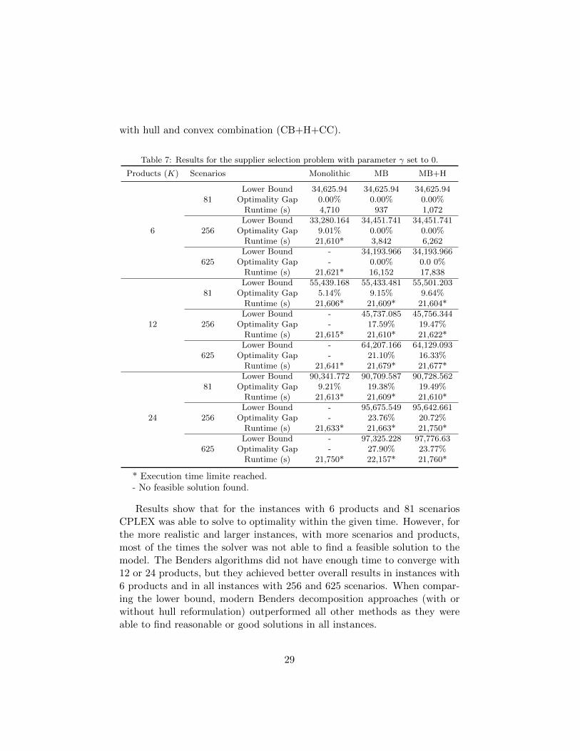
Table 7: Results for the supplier selection problem with parameter γ set to 0.

Products (K) Scenarios Monolithic MB MB+H

6

Lower Bound 34,625.94 34,625.94 34,625.9481 Optimality Gap 0.00% 0.00% 0.00%

Runtime (s) 4,710 937 1,072Lower Bound 33,280.164 34,451.741 34,451.741

256 Optimality Gap 9.01% 0.00% 0.00%Runtime (s) 21,610* 3,842 6,262

Lower Bound - 34,193.966 34,193.966625 Optimality Gap - 0.00% 0.0 0%

Runtime (s) 21,621* 16,152 17,838

12


Runtime (s) 21,606* 21,609* 21,604*Lower Bound - 45,737.085 45,756.344

256 Optimality Gap - 17.59% 19.47%Runtime (s) 21,615* 21,610* 21,622*

Lower Bound - 64,207.166 64,129.093625 Optimality Gap - 21.10% 16.33%

Runtime (s) 21,641* 21,679* 21,677*

24





Runtime (s) 21,750* 22,157* 21,760*

* Execution time limite reached.- No feasible solution found.

Results show that for the instances with 6 products and 81 scenariosCPLEX was able to solve to optimality within the given time. However, forthe more realistic and larger instances, with more scenarios and products,most of the times the solver was not able to find a feasible solution to themodel. The Benders algorithms did not have enough time to converge with12 or 24 products, but they achieved better overall results in instances with6 products and in all instances with 256 and 625 scenarios. When compar-ing the lower bound, modern Benders decomposition approaches (with orwithout hull reformulation) outperformed all other methods as they wereable to find reasonable or good solutions in all instances.

29

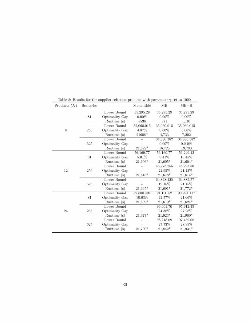
Table 8: Results for the supplier selection problem with parameter γ set to 1000.

Products (K) Scenarios Monolithic MB MB+H

6


Runtime (s) 5538 971 1,101Lower Bound 35,060.015 35,060.015 35,060.015

256 Optimality Gap 4.87% 0.00% 0.00%Runtime (s) 21608* 4,733 7,202

Lower Bound - 34,880.382 34,880.382625 Optimality Gap - 0.00% 0.0 0%

Runtime (s) 21,622* 16,725 19,798

12





Runtime (s) 21,645* 21,691* 21,772*

24





Runtime (s) 21,700* 21,842* 21,931*

30

Although Benders decomposition achieved better solutions in almost ev-ery case, it was not able to obtain good upper bounds in instances with alarger number of products, which resulted in higher GAPs. This may becaused by the structure and the size of the model, and also by the slowconvergence of benders decomposition in some cases (You and Grossmann,2013).

When compared with classical Benders decomposition, modern Bendersdecomposition achieved better convergence in all instances. This can beexplained by the faster solving time of the master problem and also by theusage of only one single exploration tree, in a way that it is not necessaryto create a search tree and revisit the same nodes in each iteration.

The other acceleration techniques did not perform as well as expected.Convex combination was not able to improve the convergence and in in-stances with 256 and 625 scenarios, it reached the total amount of memoryallowed in the first iterations. Nonetheless, we can not conclude that thesemethods are not effective for other models or instances. In instances withmore products, the hull reformulation constraints were able to improve theoptimality gap of the solutions.

The solution performance of all approaches seems to decrease when theparameter γ changes from 0 to 1000. This is line with the work of Miller andRuszczynski (2011) which shows that the more traditional decompositionalgorithms have a better performance for risk-neutral models (γ = 0) ratherthan for risk-averse ones (γ = 1000).

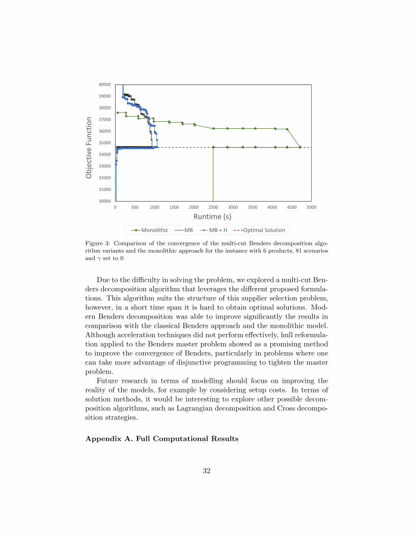
Figure 3 shows the convergence of the upper and lower bound for themulti-cut Benders decomposition algorithm variants and the monolithic ap-proach when solving the instance with 6 products, 81 scenarios and γ set to0. In this case, the modern Benders approach had a faster convergence thanother variants of Benders and than the monolithic approach.

7. Conclusions and Future Work

This paper proposes a novel formulation to tackle the integrated decisionof supplier selection and production-distribution planning for processed foodsupply chains. Uncertainty is present in the suppliers’ processes namely inlead time, availability and spot price, and in customers’ demand, which fur-thermore depends on the age of the sold product. Results show that onlyby taking such an integrated approach of tactical and strategic levels it ispossible to make better decisions regarding sourcing of perishable raw ma-terials to produce processed food products. The advantages of the premiumprice customers are willing to pay is undervalued by decoupled approaches.

31

30000

31000

32000

33000

34000

35000

36000

37000

38000

39000

40000

0 500 1000 1500 2000 2500 3000 3500 4000 4500 5000

Ob

ject

ive

Fun

ctio

n

Runtime (s)

Monolithic MB MB + H Optimal Solution

Figure 3: Comparison of the convergence of the multi-cut Benders decomposition algo-rithm variants and the monolithic approach for the instance with 6 products, 81 scenariosand γ set to 0

Due to the difficulty in solving the problem, we explored a multi-cut Ben-ders decomposition algorithm that leverages the different proposed formula-tions. This algorithm suits the structure of this supplier selection problem,however, in a short time span it is hard to obtain optimal solutions. Mod-ern Benders decomposition was able to improve significantly the results incomparison with the classical Benders approach and the monolithic model.Although acceleration techniques did not perform effectively, hull reformula-tion applied to the Benders master problem showed as a promising methodto improve the convergence of Benders, particularly in problems where onecan take more advantage of disjunctive programming to tighten the masterproblem.

Future research in terms of modelling should focus on improving thereality of the models, for example by considering setup costs. In terms ofsolution methods, it would be interesting to explore other possible decom-position algorithms, such as Lagrangian decomposition and Cross decompo-sition strategies.

Appendix A. Full Computational Results

32

Table

9:

Inst

ance

wit

h6

pro

duct

sand

81

scen

ari

os

Pro

du

cts

γS

cen

ario

sL

ower

Bou

nd

Up

per

Bou

nd

Gap

Tim

e#

Iter

atio

ns

60

81

Mon

olit

hic

34,6

25.9

434

,625

.94

0.00

%4,

710.

27-

CB

34,2

96.5

834

,790

.36

1.42

%21

,760

.88

431

CB

+H

34,3

75.1

635

,029

.88

1.87

%21

,640

.94

372

CB

+C

C33

,610

.70

35,3

95.6

95.

04%

21,6

63.2

018

5C

B+

H+

CC

33,5

35.9

735

,392

.65

5.25

%22

,131

.42

210

MB

34,6

25.9

434

,625

.94

0.00

%93

6.97

297

MB

+H

34,6

25.9

434

,625

.94

0.00

%1,

071.

8137

3M

B+

CC

34,6

25.9

434

,625

.94

0.00

%8,

427.

8129

6M

B+

H+

CC

34,6

25.9

434

,625

.94

0.00

%11

,223

.45

368

610

0081

Mon

olit

hic

35,2

95.2

935

,295

.29

0.00

%5,

538.

30-

CB

35,1

27.9

435

,589

.97

1.30

%21

,729

.64

431

CB

+H

34,8

91.6

235

,803

.53

2.55

%21

,666

.42

369

CB

+C

C34

,057

.49

36,2

39.2

26.

02%

21,6

16.1

717

8C

B+

H+

CC

33,5

62.7

136

,241

.16

7.39

%21

,654

.41

197

MB

35,2

95.2

935

,295

.29

0.00

%97

1.27

341

MB

+H

35,2

95.2

935

,295

.29

0.00

%1,

100.

9332

6M

B+

CC

35,2

95.2

935

,295

.29

0.00

%9,

223.

3331

9M

B+

H+

CC

35,2

95.2

935

,295

.29

0.00

%11

,142

.54

389

33

Table

10:

Inst

ance

wit

h6

pro

duct

sand

256

scen

ari

os

Pro

du

cts

γS

cen

ario

sL

ower

Bou

nd

Up

per

Bou

nd

Gap

Tim

e#

Iter

atio

ns

60

256

Mon

olit

hic

33,2

80.1

636

,576

.38

9.01

%21

,609

.53

-C

B33

,115

.09

36,1

05.1

28.

28%

21,7

65.3

919

0C

B+

H33

,538

.78

35,7

90.1

66.

29%

21,6

47.5

818

7C

B+

CC

26,6

82.8

738

,022

.24

29.8

2%24

,217

.46

35C

B+

H+

CC

28,0

83.3

337

,736

.18

25.5

8%21

,944

.72

40M

B34

,451

.74

34,4

51.7

40.

00%

3,84

2.05

285

MB

+H

34,4

51.7

434

,451

.74

0.00

%6,

262.

1341

0M

B+

CC

34,4

51.7

439

,907

.50

13.6

7%21

,895

.63

65M

B+

H+

CC

34,4

29.8

438

,287

.25

10.0

7%21

,838

.79

70

610

0025

6

Mon

olit

hic

35,0

60.0

236

,854

.03

4.87

%21

,608

.35

-C

B33

,600

.90

36,8

92.3

58.

92%

21,6

98.7

918

6C

B+

H32

,903

.77

37,0

35.9

811

.16%

32,3

25.7

718

8C

B+

CC

29,4

71.3

738

,839

.82

24.1

2%*

30C

B+

H+

CC

28,5

06.7

538

,688

.55

26.3

2%25

,079

.78

45M

B35

,060

.02

35,0

60.0

20.

00%

4,73

3.58

347

MB

+H

35,0

60.0

235

,060

.02

0.00

%7,

202.

2244

8M

B+

CC

35,0

60.0

239

,913

.96

12.1

6%22

,077

.57

80M

B+

H+

CC

27,4

91.6

146

,625

.42

41.0

4%21

,600

.00

5

*E

xec

uti

onre

ach

edth

eto

tal

amou

nt

of

mem

ory

all

owed

.

34

Table

11:

Inst

ance

wit

h6

pro

duct

sand

625

scen

ari

os

Pro

du

cts

γS

cen

ario

sL

ower

Bou

nd

Up

per

Bou

nd

Gap

Tim

e#

Iter

atio

ns

60

625

Mon

olit

hic

--

-21

,621

.15

-C

B33

,036

.91

35,9

23.0

28.

03%

21,8

76.0

711

3C

B+

H32

,945

.15

35,9

99.7

88.

49%

21,7

31.7

010

1C

B+

CC

26,0

53.6

942

,374

.80

38.5

2%*

5C

B+

H+

CC

26,0

53.6

943

,160

.81

39.6

4%*

5M

B34

,193

.97

34,1

93.9

70.

00%

16,1

52.4

036

0M

B+

H34

,193

.97

34,1

93.9

70.

00%

17,8

37.9

429

1M

B+

CC

26,0

53.6

943

,247

.82

39.7

6%*

5M

B+

H+

CC

33,9

22.8

544

,814

.07

24.3

0%*

13

610

0062

5

Mon

olit

hic

--

-21

,621

.67

-C

B32

,497

.52

37,0

15.7

512

.21%

21,8

37.1

711

4C

B+

H31

,908

.47

37,2

70.9

414

.39%

21,8

58.0

898

CB

+C

C24

,549

.19

43,0

23.6

642

.94%

*5

CB

+H

+C

C24

,549

.19

44,3

32.1

944

.62%

*5

MB

34,8

80.3

834

,880

.38

0.00

%16

,724

.76

356

MB

+H

34,8

80.3

834

,880

.38

0.00

%19

,797

.74

314

MB

+C

C24

,549

.19

44,3

80.2

344

.68%

*5

MB

+H

+C

C27

,491

.61

46,6

25.4

241

.04%

*5

*E

xec

uti

onre

ach

edth

eto

tal

amou

nt

of

mem

ory

all

owed

.

35

Table

12:

Inst

ance

wit

h12

pro

duct

sand

81

scen

ari

os

Pro

du

cts

γS

cen

ario

sL

ower

Bou

nd

Up

per

Bou

nd

Gap

Tim

e#

Iter

atio

ns

120

81

Mon

olit

hic

55,4

39.1

758

,442

.98

5.14

%21

,605

.66

-C

B50

,484

.34

64,6

81.7

021

.95%

21,6

66.2

944

2C

B+

H51

,102

.18

63,8

31.8

519

.94%

21,7

72.8

250

7C

B+

CC

46,6

32.9

763

,709

.48

26.8

0%22

,516

.73

130

CB

+H

+C

C44

,675

.22

63,5

71.2

529

.72%

22,2

05.1

615

0M

B55

,433

.48

61,0

17.3

49.

15%

21,6

08.6

52,

115

MB

+H

55,5

01.2

061

,424

.72

9.64

%21

,604

.37

1,73

5M

B+

CC

55,4

19.7

763

,297

.14

12.4

5%21

,652

.34

315

MB

+H

+C

C55

,439

.17

62,0

56.8

310

.66%

21,6

36.8

532

0

1210

0081

Mon

olit

hic

56,1

69.7

759

,169

.07

5.07

%21

,605

.96

-C

B52

,134

.08

65,2

99.0

820

.16%

21,6

96.0

345

8C

B+

H51

,734

.74

65,1

87.0

220

.64%

21,6

65.7

744

7C

B+

CC

47,8

01.5

164

,095

.92

25.4

2%21

,934

.02

105

CB

+H

+C

C45

,910

.74

64,0

88.1

228

.36%

21,8

77.9

914

5M

B56

,169

.77

61,3

25.3

88.

41%

21,6

04.8

91,

930

MB

+H

56,2

49.4

262

,815

.97

10.4

5%21

,603

.88

1,78

3M

B+

CC

56,1

69.7

764

,297

.71

12.6

4%21

,604

.13

305

MB

+H

+C

C56

,175

.02

62,7

43.2

910

.47%

22,2

86.5

124

5

36

Table

13:

Inst

ance

wit

h12

pro

duct

sand

256

scen

ari

os

Pro

du

cts

γS

cen

ario

sL

ower

Bou

nd

Up

per

Bou

nd

Gap

Tim

e#

Iter

atio

ns

120

256

Mon

olit

hic

--

-21

,615

.41

-C

B36

,621

.68

59,5

48.0

238

.50%

21,8

10.6

720

4C

B+

H35

,477

.93

60,7

08.3

741

.56%

21,7

69.3

217

1C

B+

CC

34,6

29.3

263

,396

.40

45.3

8%*

5C

B+

H+

CC

34,6

29.3

255

,975

.29

38.1

3%*

15M

B45

,737

.09

55,4

97.6

217

.59%

21,6

10.2

767

0M

B+

H45

,756

.34

56,8

20.7

319

.47%

21,6

21.6

649

6M

B+

CC

34,6

29.3

263

,927

.58

45.8

3%*

10M

B+

H+

CC

44,9

63.0

063

,587

.85

29.2

9%23

,496

.69

20

1210

0025

6

Mon

olit

hic

--

-21

,617

.57

-C

B39

,200

.11

59,8

88.9

134

.55%

21,6

13.6

022

4C

B+

H36

,880

.65

61,0

64.9

139

.60%

21,9

09.6

717

1C

B+

CC

30,7

01.4

257

,631

.58

46.7

3%*

5C

B+

H+

CC

30,7

01.4

257

,296

.91

46.4

2%23

,881

.59

15M

B46

,273

.26

60,0

55.0

422

.95%

21,6

78.0

652

7M

B+

H46

,293

.80

58,9

18.9

521

.43%

21,6

14.1

045

2M

B+

CC

45,7

06.4

065

,412

.08

30.1

3%*

29M

B+

H+

CC

30,7

01.4

265

,371

.93

53.0

4%*

10

*E

xec

uti

onre

ach

edth

eto

tal

amou

nt

of

mem

ory

all

owed

.

37

Table

14:

Inst

ance

wit

h12

pro

duct

sand

625

scen

ari

os

Pro

du

cts

γS

cen

ario

sL

ower

Bou

nd

Up

per

Bou

nd

Gap

Tim

e#

Iter

atio

ns

120

625

Mon

olit

hic

--

-21

,641

.11

-C

B44

,141

.80

80,8

24.7

045

.39%

21,9

31.6

112

1C

B+

H42

,989

.67

81,3

43.9

047

.15%

21,9

23.2

912

7C

B+

CC

42,5

40.5

483

,548

.43

49.0

8%*

5C

B+

H+

CC

42,5

40.5

484

,250

.43

49.5

1%*

5M

B64

,207

.17

81,3

76.8

721

.10%

21,6

78.9

226

0M

B+

H64

,129

.09

76,6

47.6

916

.33%

21,6

77.1

927

2M

B+

CC

42,5

40.5

484

,494

.45

49.6

5%*

5M

B+

H+

CC

42,5

40.5

484

,264

.90

49.5

2%*

5

1210

0062

5

Mon

olit

hic

--

-21

,645

.42

-C

B45

,328

.80

83,0

39.4

345

.41%

21,7

44.5

411

5C

B+

H44

,680

.32

83,7

37.9

046

.64%

21,8

95.0

113

1C

B+

CC

39,7

60.2

385

,350

.90

53.4

2%*

5C

B+

H+

CC

39,6

68.2

586

,634

.98

54.2

1%*

5M

B64

,848

.43

80,2

05.0

519

.15%

21,6

90.8

825

2M

B+

H64

,885

.77

82,2

87.1

121

.15%

21,7

71.5

623

9M

B+

CC

39,7

60.2

386

,512

.37

54.0

4%*

5M

B+

H+

CC

39,6

68.2

588

,640

.02

55.2

5%*

5

*E

xec

uti

onre

ach

edth

eto

tal

amou

nt

of

mem

ory

all

owed

.

38

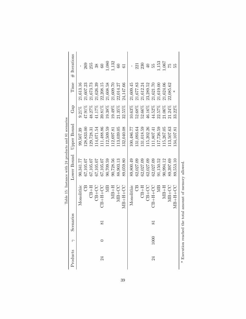
Table

15:

Inst

ance

wit

h24

pro

duct

sand

81

scen

ari

os

Pro

du

cts

γS

cen

ario

sL

ower

Bou

nd

Up

per

Bou

nd

Gap

Tim

e#

Iter

atio

ns

240

81

Mon

olit

hic

90,3

41.7

799

,507

.39

9.21

%21

,613

.16

-C

B67

,105

.07

128,

833.

0047

.91%

21,6

07.2

326

9C

B+

H67

,105

.07

129,

728.

3148

.27%

21,6

73.7

325

5C

B+

CC

67,1

05.0

711

4,07

1.54

41.1

7%21

,626

.39

38C

B+

H+

CC

67,1

05.0

711

1,48

8.86

39.8

1%22

,208

.15

60M

B90

,709

.59

112,

509.

5919

.38%

21,6

08.5

81,

080

MB

+H

90,7

28.5

611

2,69

7.81

19.4

9%21

,609

.70

1,13

2M

B+

CC

88,9

03.1

311

3,03

9.05

21.3

5%22

,014

.27

60M

B+

H+

CC

89,0

59.8

013

2,04

0.08

32.5

5%24

,147

.66

61

2410

0081

Mon

olit

hic

89,8

00.4

910

0,48

6.77

10.6

3%21

,609

.45

-C

B62

,027

.09

131,

093.

6452

.68%

21,6

77.8

322

1C

B+

H62

,027

.09

131,

018.

5952

.66%

21,6

12.2

423

0C

B+

CC

62,0

27.0

911

5,20

2.26

46.1

6%23

,289

.52

40C

B+

H+

CC

62,0

27.0

911

1,80

7.41

44.5

2%21

,621

.70

55M

B91

,150

.52

117,

726.

5922

.57%

21,6

19.0

01,

153

MB

+H

90,9

94.1

211

5,26

7.05

21.0

6%21

,624

.06

1,06

7M

B+

CC

89,3

97.6

911

3,50

7.63

21.2

4%22

,085

.62

75M

B+

H+

CC

89,5

53.1

013

4,10

7.81

33.2

2%*

55

*E

xec

uti

onre

ach

edth

eto

tal

amou

nt

of

mem

ory

all

owed

.

39

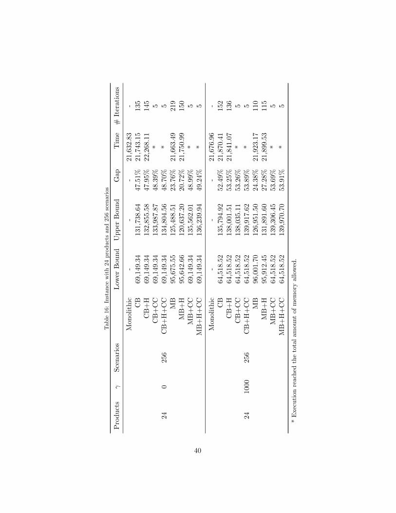
Table

16:

Inst

ance

wit

h24

pro

duct

sand

256

scen

ari

os

Pro

du

cts

γS

cen

ario

sL

ower

Bou

nd

Up

per

Bou

nd

Gap

Tim

e#

Iter

atio

ns

240

256

Mon

olit

hic

--

-21

,632

.83

-C

B69

,149

.34

131,

738.

6447

.51%

21,7

43.1

513

5C

B+

H69

,149

.34

132,

855.

5847

.95%

22,2

68.1

114

5C

B+

CC

69,1

49.3

413

3,98

7.87

48.3

9%*

5C

B+

H+

CC

69,1

49.3

413

4,80

4.56

48.7

0%*

5M

B95

,675

.55

125,

488.

5123

.76%

21,6

63.4

921

9M

B+

H95

,642

.66

120,

637.

2020

.72%

21,7

50.9

915

0M

B+

CC

69,1

49.3

413

5,56

2.01

48.9

9%*

5M

B+

H+

CC

69,1

49.3

413

6,23

9.94

49.2

4%*

5

2410

0025

6

Mon

olit

hic

--

-21

,676

.96

-C

B64

,518

.52

135,

794.

9252

.49%

21,8

70.4

115

2C

B+

H64

,518

.52

138,

001.

5153

.25%

21,8

41.0

713

6C

B+

CC

64,5

18.5

213

8,03

5.11

53.2

6%*

5C

B+

H+

CC

64,5

18.5

213

9,91

7.62

53.8

9%*

5M

B96

,001

.70

126,

951.

5024

.38%

21,9

23.1

711

0M

B+

H95

,912

.45

131,

891.

6027

.28%

21,8

99.5

311

5M

B+

CC

64,5

18.5

213

9,30

6.45

53.6

9%*

5M

B+

H+

CC

64,5

18.5

213

9,97

0.70

53.9

1%*

5

*E

xec

uti

onre

ach

edth

eto

tal

amou

nt

of

mem

ory

all

owed

.

40

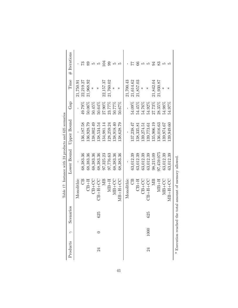
Table

17:

Inst

ance

wit

h24

pro

duct

sand

625

scen

ari

os

Pro

du

cts

γS

cen

ario

sL

ower

Bou

nd

Up

per

Bou

nd

Gap

Tim

e#

Iter

atio

ns

240

625

Mon

olit

hic

--

-21

,750

.91

-C

B68

,383

.36

136,

187.

5849

.79%

22,2

19.2

773

CB

+H

68,3

83.3

613

6,92

8.79

50.0

6%21

,968

.92

89C

B+

CC

68,3

83.3

613

8,00

2.49

50.4

5%*

5C

B+

H+

CC

68,3

83.3

613

8,53

4.54

50.6

4%*

5M

B97

,325

.23

134,

981.

1427

.90%

22,1

57.3

710

4M

B+

H97

,776

.63

128,

259.

2423

.77%

21,7

60.0

299

MB

+C

C68

,383

.36

138,

918.

4050

.77%

*5

MB

+H

+C

C68

,383

.36

138,

628.

7950

.67%

*5

2410

0062

5

Mon

olit

hic

--

-21

,700

.43

-C

B63

,012

.39

137,

238.

4754

.09%

21,6

14.6

277

CB

+H

63,0

12.3

913

8,33

5.81

54.4

5%21

,857

.03

66C

B+

CC

63,0

12.3

913

9,27

4.51

54.7

6%*

5C

B+

H+

CC

63,0

12.3

913

9,77

3.61

54.9

2%*

5M

B98

,215

.09

135,

906.

1927

.73%

21,8

42.0

494

MB

+H

97,4

59.0

7513

6,01

6.63

28.3

5%21

,930

.87

83M

B+

CC

63,0

12.3

913

9,97

4.67

54.9

8%*

5M

B+

H+

CC

63,0

12.3

913

9,94

9.60

54.9

7%*

5

*E

xec

uti

onre

ach

edth

eto

tal

amou

nt

of

mem

ory

all

owed

.

41

Acknowledgments

This work is financed by the ERDF – European Regional DevelopmentFund through the COMPETE Programme (operational programme for com-petitiveness) and by National Funds through the FCT – Fundacao para aCiencia e a Tecnologia (Portuguese Foundation for Science and Technology)within project “FCOMP-01-0124-FEDER-041499”. The first author wouldlike also to acknowledge the support of the CMU-Portugal Programme.

References

Ahumada O, Villalobos JR (2009) Application of planning models in theagri-food supply chain: A review. European Journal of Operational Re-search 196(1):1–20

Aissaoui N, Haouari M, Hassini E (2007) Supplier selection and order lotsizing modeling: A review. Computers & operations research 34(12):3516–3540

Amorim P, Alem D, Almada-Lobo B (2013a) Risk management in produc-tion planning of perishable goods. Industrial & Engineering ChemistryResearch 52(49):17,538–17,553

Amorim P, Costa A, Almada-Lobo B (2013b) Influence of consumer pur-chasing behaviour on the production planning of perishable food. ORSpectrum pp 1–24

Ata B, Lee D, Tongarlak MH (2012) Got Local Food? Harvard BusinessSchool, Working Paper

Balas E (1985) Disjunctive programming and a hierarchy of relaxationsfor discrete optimization problems. SIAM Journal on Algebraic DiscreteMethods 6(3):466–486

Benders JF (1962) Partitioning procedures for solving mixed-variables pro-gramming problems. Numerische mathematik 4(1):238–252

Birge J, Louveaux F (1997) Introduction to stochastic programmingspringer-verlag. New York

Birge JR, Louveaux FV (1988) A multicut algorithm for two-stage stochasticlinear programs. European Journal of Operational Research 34(3):384–392

42

Castro PM, Grossmann IE (2012) Generalized disjunctive programming asa systematic modeling framework to derive scheduling formulations. In-dustrial & Engineering Chemistry Research 51(16):5781–5792

Chen J, Guo Z (2013) Strategic sourcing in the presence of uncertain supplyand retail competition. Production and Operations Management

Choudhary D, Shankar R (2014) A goal programming model for joint deci-sion making of inventory lot-size, supplier selection and carrier selection.Computers & Industrial Engineering 71:1–9

De Boer L, Labro E, Morlacchi P (2001) A review of methods supportingsupplier selection. European Journal of Purchasing & Supply Management7(2):75–89

Deng X, Hu Y, Deng Y, Mahadevan S (2014) Supplier selection using AHPmethodology extended by D numbers. Expert Systems with Applications41(1):156–167

Ding H, Benyoucef L, Xie X (2005) A simulation optimization methodologyfor supplier selection problem. International Journal of Computer Inte-grated Manufacturing 18(2-3):210–224

Federgruen A, Yang N (2008) Selecting a portfolio of suppliers under demandand supply risks. Operations Research 56(4):916–936

FoodDrink Europe (2014) Data & trends of the eu-ropean food and drink industy 2013-2014. URLhttp://www.fooddrinkeurope.eu/S=0/publication/data-trends-of-the-european-food-and-drink-industry-2013-2014/

Frash RE, DiPietro R, Smith W (2014) Pay more for mclocal? examin-ing motivators for willingness to pay for local food in a chain restaurantsetting. Journal of Hospitality Marketing & Management

Fu Q, Lee CY, Teo CP (2010) Procurement management using optioncontracts: random spot price and the portfolio effect. IIE Transactions42(11):793–811

Grossmann IE, Trespalacios F (2013) Systematic modeling of discrete-continuous optimization models through generalized disjunctive program-ming. AIChE Journal 59(9):3276–3295

43

Guo C, Li X (2014) A multi-echelon inventory system with supplier selectionand order allocation under stochastic demand. International Journal ofProduction Economics 151:37–47

Hammami R, Temponi C, Frein Y (2014) A scenario-based stochastic modelfor supplier selection in global context with multiple buyers, currencyfluctuation uncertainties, and price discounts. European Journal of Oper-ational Research 233(1):159–170

Ho W, Xu X, Dey PK (2010) Multi-criteria decision making approaches forsupplier evaluation and selection: A literature review. European Journalof Operational Research 202(1):16–24

Hong Z, Lee C (2013) A decision support system for procurement riskmanagement in the presence of spot market. Decision Support Systems55(1):67–78

Kumar A, Jain V, Kumar S (2014) A comprehensive environment friendlyapproach for supplier selection. Omega 42(1):109–123

Lee S, Grossmann IE (2000) New algorithms for nonlinear generalized dis-junctive programming. Computers & Chemical Engineering 24(9):2125–2141

Maloni MJ, Brown ME (2006) Corporate social responsibility in the supplychain: an application in the food industry. Journal of business ethics68(1):35–52

Martinez S (2010) Local food systems; concepts, impacts, and issues. 97,Diane Publishing

Miller N, Ruszczynski A (2011) Risk-averse two-stage stochastic linear pro-gramming: modeling and decomposition. Operations research 59(1):125–132

Nemhauser GL, Wolsey LA (1988) Integer and combinatorial optimization,vol 18. Wiley New York

Oberholtzer L, Dimitri C, Jaenicke EC (2014) Examining US Food Retailers’Decisions to Procure Local and Organic Produce From Farmer Direct-to-Retail Supply Chains. Journal of Food Products Marketing 20(4):345–361

Qian L (2014) Market-based supplier selection with price, delivery time,and service level dependent demand. International Journal of ProductionEconomics 147:697–706

44

Rajurkar SW, Jain R (2011) Food supply chain management: review, clas-sification and analysis of literature. International Journal of IntegratedSupply Management 6(1):33–72

Raman R, Grossmann IE (1994) Modelling and computational techniquesfor logic based integer programming. Computers & Chemical Engineering18(7):563–578

Rockafellar RT, Uryasev S (2000) Optimization of conditional value-at-risk.Journal of risk 2:21–42

Rockafellar RT, Uryasev S (2002) Conditional value-at-risk for general lossdistributions. Journal of Banking & Finance 26(7):1443–1471

Santoso T, Ahmed S, Goetschalckx M, Shapiro A (2005) A stochastic pro-gramming approach for supply chain network design under uncertainty.European Journal of Operational Research 167(1):96–115

Sarykalin S, Serraino G, Uryasev S (2008) Value-at-risk vs. conditional value-at-risk in risk management and optimization. Tutorials in Operations Re-search INFORMS, Hanover, MD

Sawik T (2013) Integrated selection of suppliers and scheduling of customerorders in the presence of supply chain disruption risks. International Jour-nal of Production Research 51(23-24):7006–7022

Schonhart M, Penker M, Schmid E (2009) Sustainable local food productionand consumption: challenges for implementation and research. Outlookon agriculture 38(2):175–182

Sevkli M, Koh SL, Zaim S, Demirbag M, Tatoglu E (2008) Hybrid analyticalhierarchy process model for supplier selection. Industrial Management &Data Systems 108(1):122–142

Shapiro A, Homem-de Mello T (1998) A simulation-based approach to two-stage stochastic programming with recourse. Mathematical Programming81(3):301–325

Silbermayr L, Minner S (2014) A multiple sourcing inventory model underdisruption risk. International Journal of Production Economics 149:37–46

Smith BC (2004) Robust airline fleet assignment. Georgia Institute of Tech-nology, PhD Thesis

45

Thorsteinsson ES (2001) Branch-and-check: A hybrid framework integrat-ing mixed integer programming and constraint logic programming. In:Principles and Practice of Constraint Programming–CP 2001, Springer,pp 16–30

Van Donselaar K, van Woensel T, Broekmeulen R, Fransoo J (2006) In-ventory control of perishables in supermarkets. International Journal ofProduction Economics 104(2):462–472

Van Slyke RM, Wets R (1969) L-shaped linear programs with applicationsto optimal control and stochastic programming. SIAM Journal on AppliedMathematics 17(4):638–663

Wallace SW, Ziemba WT (2005) Applications of stochastic programming,vol 5. Siam

Wets R (1983) Stochastic programming: Solution techniques and approxi-mation schemes. Springer

Williams HP (1999) Model building in mathematical programming. Wiley

You F, Grossmann IE (2013) Multicut benders decomposition algorithm forprocess supply chain planning under uncertainty. Annals of OperationsResearch 210(1):191–211

46

supplier selection for supply chains in the processed...

Documents