Supply and Demand Analysis

for Residential Properties

Objectives of Chapter:

Discuss the methods that can be used to estimate housing demand.

* Estimating demand in general * Local survey-based methods

Expected learning results:

Main factors in estimating demand for residential properties in general;

Apply some methods of estimating demand for residential properties.

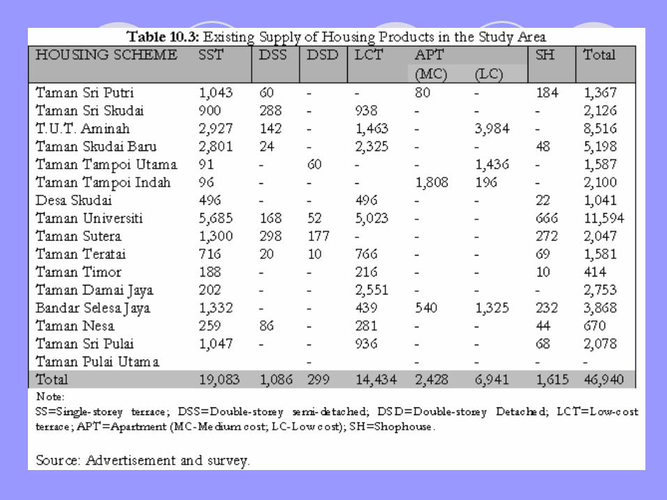
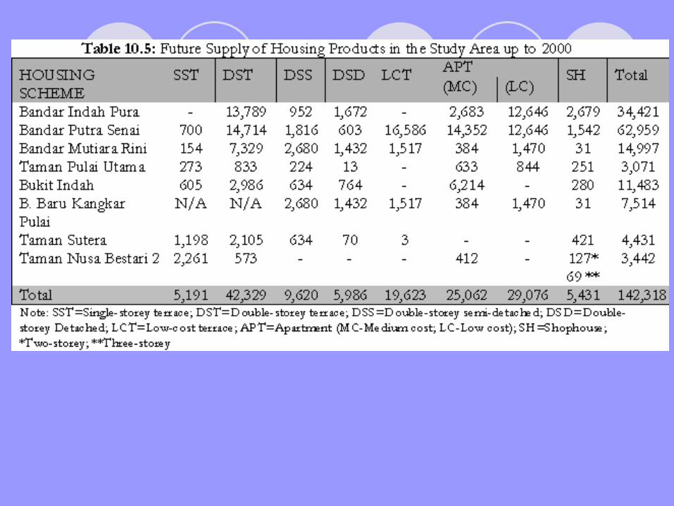
Analysing Supply

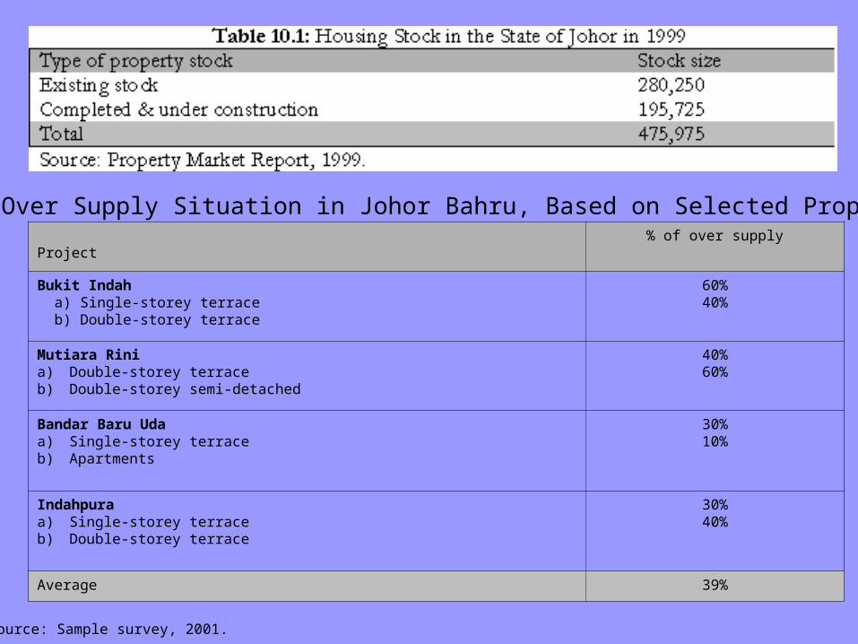
Table 10.2: Over Supply Situation in Johor Bahru, Based on Selected Property Projects

Project% of over supply

Bukit Indah a) Single-storey terrace b) Double-storey terrace

60%40%

Mutiara Rinia) Double-storey terraceb) Double-storey semi-detached

40%60%

Bandar Baru Udaa) Single-storey terraceb) Apartments

30%10%

Indahpuraa) Single-storey terraceb) Double-storey terrace

30%40%

Average 39%

Source: Sample survey, 2001.

Methods of Estimating

Residential Demand

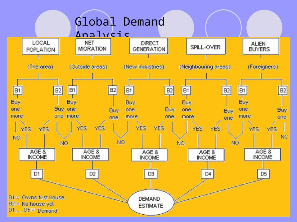
Global Demand Analysis

Total population = 100,000 Eligible age (25 – 49) = 35% Eligible population = 0.35 x 100,000 = 35,000 Employment = 97% Eligible working population = 0.97 x 35,000 = 33,950 Home ownership = 65% First-time buyer potential demand = 0.35 x 33,950 = 11,883 Buying interest: Non first-time buyers = 8% First-time buyers = 30% Overall potential demand: Non first-time buyers = 0.08 x 0.65 x 33,950 = 1,765 First-time buyers = 0.3 x 11,883 = 3,565 Total = 1,765 + 3,565 = 5,330 Income categories: Low-income = 35% Middle-income = 45% Upper income = 20% Demand by income-based market segments: Low-income segment = 0.35 x 5,330 = 1,866 Middle-income segment = 0.45 x 5,330 = 2,399 Upper-income segment = 0.20 x 5,330 = 1,066

Global Residential Demand

A town has a working population of 23,000 people. From this figure, 17% are the first-time eligible buyers while 80% of them are non first-time eligible buyers. From these two categories of buyers, 35% are targeted buyers. Entrance to the labour market is estimated to be 2.5% of the working population and 1% are potential buyers. However, only 1% of them are targeted buyers. About 3% of the population working in the town are in-migrants; 1% out of this figure are first-time buyers while 0.5% are non first-time buyers. From the Property Market Report, (PMR) it was found that alien buyers constitutes 0.2% of the total targeted domestic buyers. The information from the PMR also revealed that the market concentration of residential transaction is 64% from the total real estate transaction.

Estimate the demand for properties in the area. If current available stock is 12,000 units, assess the market situation.

Class Exercise

Answer

Let say available supply = 12,000 unitsFirst-time potential buyers = 5,330 peopleAssume: one FTPB buys one unitDD-SS balance = 5,300/12,000 = 0.44DD gap = 12,000-5,330 = 6,670 unitsExcess supply = 100-44.4% = 55.6%SS excess capacity = 6,670/5,330=125%

Severe excess supply, weak demand

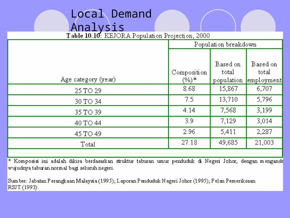
Local Demand Analysis

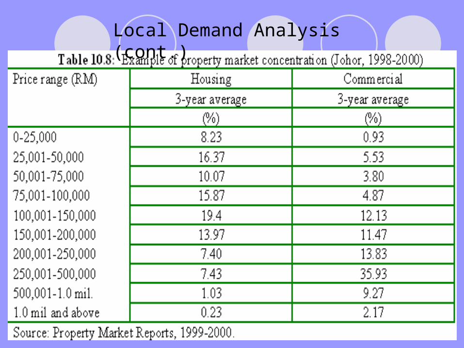
Local Demand Analysis (cont.)

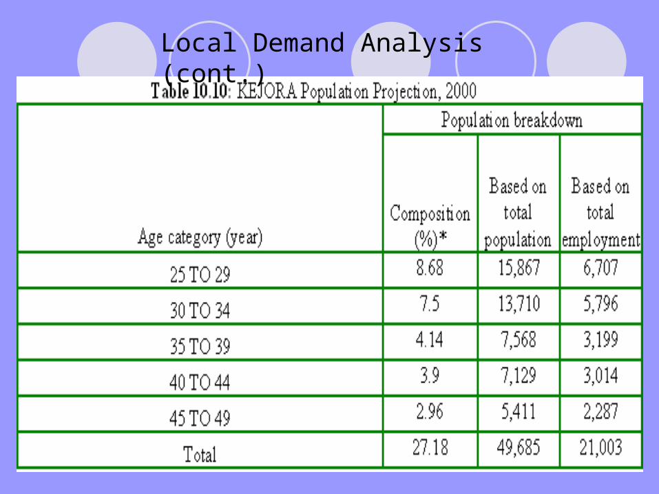
Local Demand Analysis (cont.)

Local Demand Analysis (cont.)

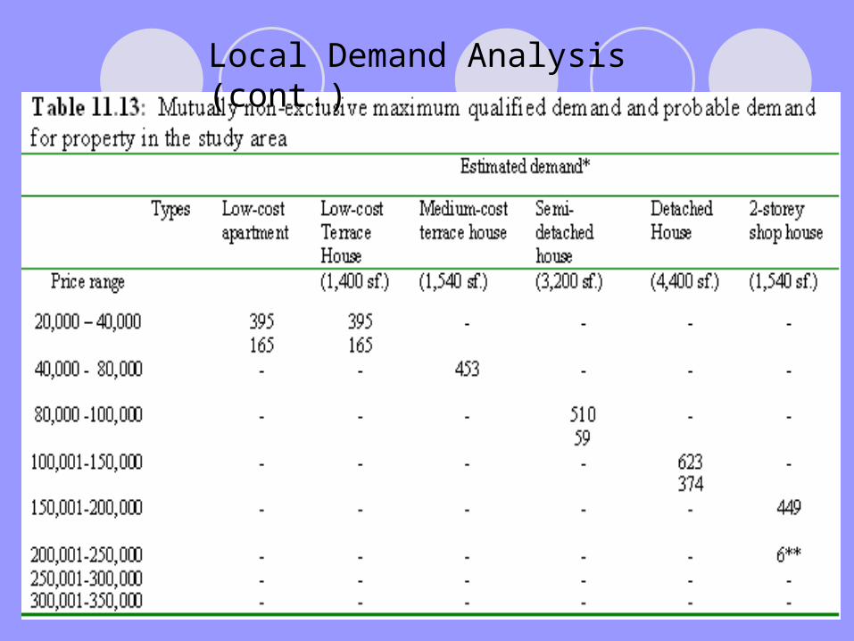
Local Demand Analysis (cont.)

Model-Based Demand Prediction

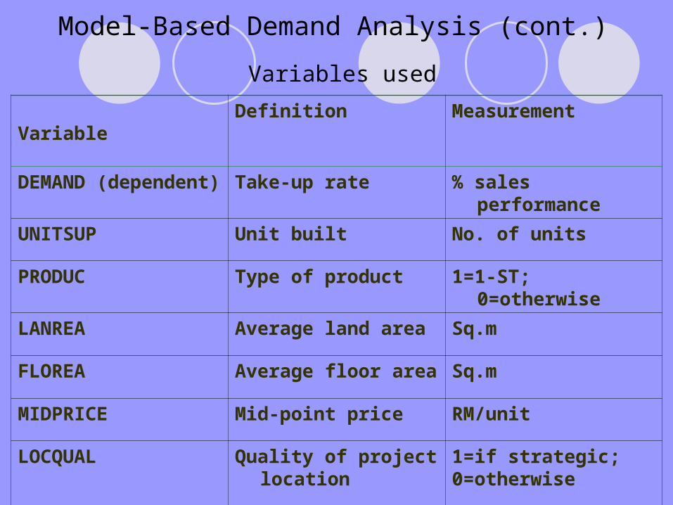
Variables used

VariableDefinition Measurement

DEMAND (dependent) Take-up rate % sales performance

UNITSUP Unit built No. of units

PRODUC Type of product 1=1-ST; 0=otherwise

LANREA Average land area Sq.m

FLOREA Average floor area Sq.m

MIDPRICE Mid-point price RM/unit

LOCQUAL Quality of project location

1=if strategic;0=otherwise

Model-Based Demand Analysis (cont.)

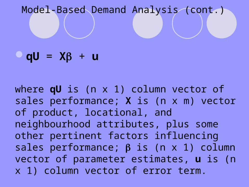
qU = X + u

where qU is (n x 1) column vector of sales performance; X is (n x m) vector of product, locational, and neighbourhood attributes, plus some other pertinent factors influencing sales performance; is (n x 1) column vector of parameter estimates, u is (n x 1) column vector of error term.

Model-Based Demand Analysis (cont.)

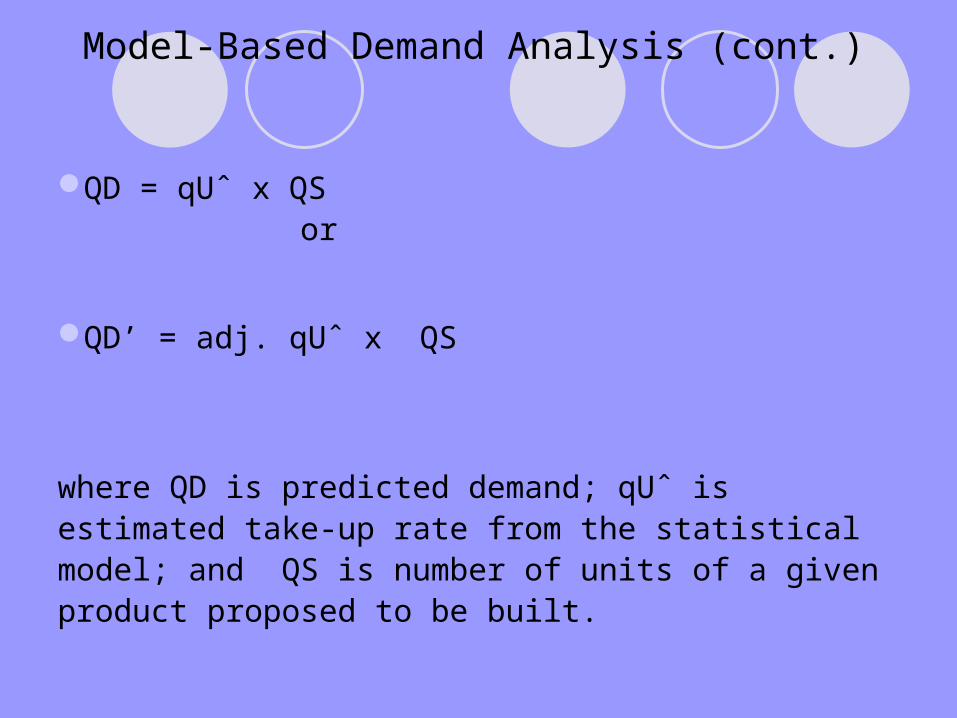
QD = qUˆ x QS or

QD’ = adj. qUˆ x QS

where QD is predicted demand; qUˆ is estimated take-up rate from the statistical model; and QS is number of units of a given product proposed to be built.

Model-Based Demand Analysis (cont.)

Qu = 71.615 + 0.002720*UNITSUP – 0.009567*LAREA – 0.001487*FLOREA – 4.506*PROD1 – 13.655*PROD2 – 11.891*PROD3

– 0.000006023*MIDPRICE + 37.438*LOCQUAL

Model-Based Demand Analysis (cont.)

Model-Based Demand Analysis (cont.)

Thank you!