supply chain coordination with different objectives · supply chain coordination with different...

SUPPLY CHAIN COORDINATION WITH

DIFFERENT OBJECTIVES

A THESIS

SUBMITTED TO THE DEPARTMENT OF INDUSTRIAL ENGINEERING

AND THE GRADUATE SCHOOL OF ENGINEERING AND SCIENCE

OF BILKENT UNIVERSITY

IN PARTIAL OF FULFILLMENT OF THE REQUIREMENTS

FOR THE DEGREE OF MASTER OF SCIENCE

By

Emre Haliloğlu

June, 2013

i

I certify that I have read this thesis and that in my opinion it is fully adequate, in scope and in

quality, as a thesis for the degree of Master of Science.

___________________________________

Prof. Dr. Nesim Erkip (Advisor)



___________________________________

Assist. Prof. Dr. Alper Şen



______________________________________

Assist. Prof. Dr. Ayşe Kocabıyıkoğlu

Approved for the Graduate School of Engineering and Science:

____________________________________

Prof. Dr. Levent Onural

Director of the Graduate School

ii

ABSTRACT

SUPPLY CHAIN COORDINATION WITH DIFFERENT OBJECTIVES

Emre Haliloğlu

M.S. in Industrial Engineering

Advisor: Prof. Nesim Erkip

June, 2013

In a typical supply chain, each party tries to optimize his/her own objective that causes the

poor total supply chain performance. By contracting on a set of transfer payments, each firm’s

objectives become aligned with the supply chain’s objective, which is called coordination;

hence the optimal result for the supply chain can be achieved. In the literature, common

treatment to supply chain coordination for the newsboy problem is to analyze the system

under the assumption that the objectives’ of the parties are expected profit maximization,

however the real life observations show that this might not be the case. Hence, this

assumption is relaxed and the supply chain coordination is studied when the objectives’ of the

parties are different than the expected profit maximization, which are probability

maximization of reaching a target profit, expected return on investment maximization and the

probability maximization of reaching a target return on investment under the wholesale price,

buy back and the revenue sharing contracts. This thesis reveals that under the assumption of

compliance, the coordination is possible for some contract types and the objectives if some

conditions are satisfied, however some contracts cannot coordinate the channel for some

objectives no matter what the conditions are.

Keywords: Supply chain coordination, newsboy problem, contract theory, objective types

different than the expected profit maximization

iii

ÖZET

FARKLI OBJEKTİFLERLE TEDARİK ZİNCİRİ KOORDİNASYONUN

İNCELENMESİ

Emre Haliloğlu

Endüstri Mühendisliği Yüksek Lisans

Tez Yöneticisi: Prof. Nesim Erkip

Haziran, 2013

Klasik tedarik zincirinde her bir parti kendi yararına olacak şekilde davranma eğilimindedir,

bu durum tedarik zincirinin toplam performansına zarar vermektedir. Değişik kontratlar

uygulayarak, her bir partinin hedefinin tedarik zinciriyle paralel olmasını sağlayarak tedarik

zincirinin toplam performansının en iyilenmesine tedarik zinciri koordinasyonu

denilmektedir. Gazeteci çocuk problemi için koordinasyonun sağlanıp sağlanmadığı

literatürde tedarik zincirindeki partilerin hedef fonksiyonlarının beklenen karı en iyilemek

varsayımı şartıyla incelenmektedir. Bu çalışmada klasik literatürden farklı olarak tedarik

zinciri partilerinin hedef fonksiyonları; belirli bir kar miktarına ulaşma ihtimalini en iyileme,

beklenen yatırım oranını en iyileme ve belirli bir yatırım oranına ulaşma ihtimalini en iyileme

olarak alınmıştır. Çalışılan kontrat tipleri ise toptan satış fiyatı üzerinden yapılan kontratlar,

satılmayan malların geri alımına ilişkin kontratlar ve alıcının sattığı her üründen elde ettiği

karın belli yüzdesini tedarikçiye vermesine ilişkin kontratlardır. Bu tezde, belirli şartların

sağlanması durumunda bazı kontratların bazı hedef fonksiyonları için tedarik zinciri

koordinasyonunu sağlayabileceğini; bazı kontratların ise bazı hedef fonksiyonları için tedarik

zinciri koordinasyonunu hiçbir şekilde sağlayamayacağı açığa çıkarılmıştır.

iv

Anahtar Kelimeler: Tedarik zinciri koordinasyonu, gazeteci çocuk problemi, kontrat teorisi,

tedarik zinciri partilerinin hedef fonksiyonları

v

ACKNOWLEDGEMENT

First and foremost, I would like to express my sincere gratitude to Prof.Nesim Erkip

for his attention, support, and valuable guidance throughout my study, as well as for his

patience and insight.

I am highly indebted to my dissertation committee, Alper Şen and Ayşe

Kocabıyıkoğlu, for accepting to read and review this thesis and for their suggestions.

I am grateful to all faculty members especially, Alper Şen, Barbaros Tansel and

Mehmet Rüştü Taner for their endless effort and support during my undergraduate and

graduate years.

I wish to express my deepest gratitude to my family for their precious and perpetual

love and support. It was such a privilege to have such a family.

Moreover, with all my heart, I would like to thank to Fatma Cansu Çelen. I always

appreciated her goodness and patience.

I would like to thank to my close friends Emre Kara, Bharadwaj Kadiyala, Sertalp

Bilal Çay and Pelin Çay for their support and friendship. Furthermore, I want to thank to Ece

Zeliha Demirci, Hatice Çalık, Zübeyde Gülce Çuhacı, Elifnur Doğruöz, Pelin Balcı, Malek

Ebadi, Ramez Kian, Ayşegül Onat, Ahmet Burak Paç,Sibel Sözüer and Ahmet Yükseltürk for

their friendship during my study.

Finally, I am also thankful to TÜBİTAK for the financial support they provided during

my research.

vi

TABLE OF CONTENTS

ABSTRACT .............................................................................................................................. ii

ÖZET ........................................................................................................................................ iii

ACKNOWLEDGEMENT ....................................................................................................... v

LIST OF FIGURES ................................................................................................................. xi

LIST OF TABLES .................................................................................................................. xii

CHAPTER 1 INTRODUCTION ................................................................................. 1

1.1 The Classical Newsvendor Problem and Extensions to Different Objectives ........... 2

1.2 Contract Types ........................................................................................................... 5

1.2.1 The Wholesale Price Contract ........................................................................ 5

1.2.2 The Buy Back Contract .................................................................................. 5

1.2.3 The Revenue Sharing Contract ...................................................................... 6

1.3 Coordination .............................................................................................................. 6

CHAPTER 2 PRELIMINARIES ................................................................................ 9

2.1 Parameters and Variables ........................................................................................... 9

2.1.1 Common Parameters and Variables ............................................................... 9

2.1.2 Variables and Parameters for the Supply Chain .......................................... 10

2.1.3 Variables and Parameters for the Retailer .................................................... 11

2.2 Additional Notation ................................................................................................. 11

2.2.1 The Notations for the Probability Maximization of Reaching a Target

Profit Level for the Supply Chain and the Retailer ...................................... 12

2.2.2 The Notations for the Probability Maximization of Reaching a Target

Return on Investment Level for the Supply Chain and the Retailer ............ 13

vii

2.3 Assumptions ............................................................................................................. 14

2.3.1 List of Assumptions ..................................................................................... 14

2.3.2 The Summary Table for the Assumptions ................................................... 16

2.3.3 The Summary Table for the Assumptions of the Coordination ................... 17

2.4 Notations of the Common Demand Distributions ................................................... 18

2.4.1 The Exponential Distribution ....................................................................... 18

2.4.2 The Gamma Distribution .............................................................................. 18

2.4.3 The Weibull Distribution ............................................................................. 19

2.4.4 The Normal Distribution .............................................................................. 19

2.4.5 The Uniform Distribution ............................................................................ 19

CHAPTER 3 CALCULATION OF THE OPTIMAL ORDER QUANTITIES

FOR THE SUPPLY CHAIN AND THE RETAILER ..................... 20

3.1 The Optimal Order Quantity when the Objective is the Probability

Maximization of Reaching a Target Profit Level .................................................... 21

3.1.1 General Formulas for the Order Quantities .................................................. 21

3.1.2 Conditions for Uniqueness ........................................................................... 23

3.2 The Optimal Order Quantity when the Objective is Expected Return on

Investment Maximization ........................................................................................ 29

3.2.1 General Formulas for the Optimal Order Quantities .................................... 29

3.2.2 The Unique Optimal Order Quantity Conditions ......................................... 31

3.3 The Optimal Order Quantity when the Objective is the Maximization of Probability

to Reach a Target Return on Investment .................................................................. 32

3.3.1 General Formulas for the Optimal Order Quantities .................................... 32

3.3.2 The Unique Optimal Order Quantity Conditions ......................................... 34

viii

CHAPTER 4 COORDINATION FOR THE WHOLESALE PRICE,

BUY BACK AND THE REVENUE SHARING CONTRACTS .... 40

4.1 Coordination for the Probability Maximization of Reaching a Target Profit .......... 41

4.1.1 The Wholesale Price Contract: The Necessary Conditions for the

Coordination ................................................................................................. 41

4.1.2 The Buy Back and the Revenue Sharing Contracts: The Necessary

Conditions for the Coordination ................................................................... 45

4.2 Coordination for the Expected Return on Investment Maximization ...................... 51


Coordination ................................................................................................. 51



4.3 Coordination for the Probability Maximization of Reaching a Target Return on

Investment ................................................................................................................ 56


Coordination ................................................................................................. 56



4.4 Main Results of Chapter 4 ....................................................................................... 64

CHAPTER 5 MORE ON SELECTING TARGETS OF THE

SUPPLY CHAIN ................................................................................. 66

5.1 Choosing .............................................................................................................. 66

5.2 Choosing .............................................................................................................. 69

CHAPTER 6 CONCLUSION ............................................................................... 71

BIBLIOGRAPHY ................................................................................................................... 74

ix

APPENDICES ......................................................................................................................... 76

APPENDIX A .......................................................................................................................... 80

APPENDIX B ........................................................................................................................... 85

APPENDIX B-1 ....................................................................................................................... 85

APPENDIX B-2 ....................................................................................................................... 87

APPENDIX C ........................................................................................................................... 89

APPENDIX C-1 ....................................................................................................................... 89

APPENDIX C-1a ...................................................................................................................... 89

APPENDIX C-1b ..................................................................................................................... 92

APPENDIX C-2 ....................................................................................................................... 94

APPENDIX C-3 ....................................................................................................................... 96

APPENDIX C-4 ....................................................................................................................... 98

APPENDIX C-4a ...................................................................................................................... 98

APPENDIX C-4b ................................................................................................................... 100

APPENDIX C-5 ..................................................................................................................... 105

APPENDIX D ........................................................................................................................ 108

APPENDIX E ......................................................................................................................... 111

APPENDIX F ......................................................................................................................... 114

APPENDIX F-1 ...................................................................................................................... 114

APPENDIX F-2 ...................................................................................................................... 116

APPENDIX G ........................................................................................................................ 118

APPENDIX G-1 ..................................................................................................................... 118

APPENDIX G-1a ................................................................................................................... 118

APPENDIX G-1b ................................................................................................................... 120

APPENDIX G-2 ..................................................................................................................... 122

x

APPENDIX G-2a ................................................................................................................... 122

APPENDIX G-2b ................................................................................................................... 124

APPENDIX G-3 ..................................................................................................................... 125

APPENDIX G-3a ................................................................................................................... 125

APPENDIX G-3b ................................................................................................................... 127

APPENDIX G-4 ..................................................................................................................... 129

APPENDIX G-4a ................................................................................................................... 129

APPENDIX G-4b ................................................................................................................... 131

APPENDIX G-5 ..................................................................................................................... 133

APPENDIX H ........................................................................................................................ 135

APPENDIX H-1 ..................................................................................................................... 135

APPENDIX H-2 ..................................................................................................................... 137

APPENDIX H-3 ..................................................................................................................... 139

APPENDIX I .......................................................................................................................... 141

APPENDIX I-1 ....................................................................................................................... 141

APPENDIX I-2 ....................................................................................................................... 143

APPENDIX I-3 ....................................................................................................................... 145

APPENDIX J .......................................................................................................................... 147

APPENDIX J-1 ...................................................................................................................... 147

APPENDIX J-2 ...................................................................................................................... 148

xi

LIST OF FIGURES

Figure 3-1: The illustration of unique optimal order quantity for the supply chain .............. 28

Figure 3-2: The illustration of the unique optimal order quantity for the retailer for the

wholesale price contract ...................................................................................... 39

Figure 4-1: The upper bound for the retailer’s target profit in order to suffice to satisfy

the assumptions of the coordination .................................................................... 43

Figure 4-2: An example for having more than one solution for the buy back contract ......... 47

Figure 4-3: An example for the relation between wb and expected return on investment

for the buy back contract when the coordination is satisfied .............................. 55

Figure 4-4: An example for the relation between wrs and expected return on investment

for the buy back contract when the coordination is satisfied .............................. 56

Figure 5-1: The effects of the target profits on the expected profits ...................................... 68

Figure 5-2: The effects of the target profits on the expected profit ....................................... 70

xii

LIST OF TABLES

Table 2-1: Contract specific variables .................................................................................. 11

Table 2-2: Some simple notation used for the buy back and the revenue sharing contracts 12

Table 2-3: The notations for the parties for the probability maximization of reaching

a target profit level objective ............................................................................... 13

Table 2-4: The notations for the parties for the probability maximization of reaching

a target return on investment level objective ...................................................... 14

Table 2-5: The necessary assumptions for different objectives for the supply chain ........... 16

Table 2-6: The necessary assumptions for different contract types for the probability

maximization of reaching target profit for the retailer ........................................ 16

Table 2-7: The necessary assumptions for different contract types for the expected return

of investment maximization for the retailer ........................................................ 17

Table 2-8: The necessary assumptions for different contract types for the probability

maximization of reaching target return on investment for the retailer ................ 17

Table 2-9: The necessary assumptions for the coordination for different contract types

for the probability maximization of reaching target profit for the retailer .......... 17


for the expected return on investment maximization for the retailer .................. 18


for the probability maximization of reaching target return on investment for

the retailer ............................................................................................................ 18

Table 4-1: An example for the manipulation when the wholesale price contract is used .... 44

Table 4-2: Profits for the supplier for sold and unsold items with different parameters

when Rr =1000 and R=7000 ................................................................................ 49

xiii

Table 4-3: Profits for the retailer for sold and unsold items with different parameters

when Rr =1000 and R=7000 ................................................................................ 49

Table 4-4: An illustration of closure to manipulation for the buy back contract .................. 50

Table 4-5: The illustration of the manipulation for the wholesale price contract ................. 58

Table 4-6: The illustration of closure to manipulation for the buy back contract ................ 63

Table 4-7: The illustration of closure to manipulation for the revenue sharing contract ..... 63

Table 4-8: The summary table for the probability maximization of reaching a target profit65

Table 4-9: The summary table for the expected return on investment maximization .......... 65

Table 4-10: The summary table for the probability maximization of reaching a target

return on investment ............................................................................................ 65

Table 5-1: The effect of choosing a very low target profit level for the supply chain ......... 67

Table 5-2: The effect of choosing a very high target profit level for the supply chain ........ 67

Table 5-3: The effect of choosing a very low target return on investment level for the

supply chain ......................................................................................................... 69

1

CHAPTER 1 INTRODUCTION

The classical newsvendor problem is a one time business decision about determining

the number of newspaper orders that should be placed by the newsboy in order to maximize

the expected profit. Since its first formulation by Whitin (1955), the classical newsvendor

problem has found applications in a wide variety of business context such as buying style

goods for retailer, setting safety stock levels for items, selecting the right capacity for a

facility and deciding the number of overbooking customers for airline companies. All of these

newsvendor problems share a common mathematical structure. The order quantity for a single

perishable product with stochastic demand should be decided before observing the demand

for given unit, cost, selling price, salvage value and the loss of goodwill cost.

In this thesis, the same problem is examined for the supply chain and the retailer with

a change in the objective of the classical newsvendor problem; hence objectives we examine

are different than the expected profit maximization. As in the classical newsvendor problem,

there is a single perishable product with stochastic demand whose distribution is known.

Furthermore, there is one supplier and one retailer, and the retailer has a single opportunity to

place an order before observing the demand.1 The supplier has infinite capacity and she has to

produce all the orders placed by the retailer before the beginning of the selling season.2

Depending on the order quantity, contract type and parameters, there is a transfer money from

the retailer to the supplier. In order to ensure the supplier not to deviate from the order

1 The words supplier, manufacturer and the vendor can be used interchangeably. We choose supplier and use

it throughout the thesis.

2 In this work, we adopt the convention that the supplier and the supply chain are female and the retailer is

male.

2

quantity, we assume that the consequences of deviating from the order quantity are severe

such as court action or loss of good reputation. This is called as compliance in the literature

(Cachon, 2003).

Additionally, both parties have no fixed costs and both parties’ variable costs do not

vary with the order quantity. Both parties have different loss of goodwill costs due to the lost

customers when the demand is higher than the quantity produced. On the other hand, there is

a salvage value when there is not enough demand for the product.

Even though two parties, one supplier and one retailer, are considered in the setting

of this thesis, there is also another person, a coordinator who suggests an order quantity,

which is optimal for the supply chain. The aim of producing exactly the optimal order

quantity of the supply chain is to make each firm no worse off and at least one party better

off. Retailer also decides his optimal order quantity according to his objective and the

parameters.3 If the optimal order quantities of the supply chain and the retailer are same and

both parties, the retailer and the supplier, are happy with the contract parameters, the supply

chain coordination is achieved.

Under the assumptions stated above, this thesis investigates the supply chain

coordination for different objectives under different contracts. What different objectives,

different contracts and coordination stand for in our work is explained consecutively in the

following subsections.

1.1 The Classical Newsvendor Problem and Extensions to

Different Objectives

In the classical newsvendor problem, the retailer and the supplier are the two parties

and the retailer has a single purchasing opportunity before the selling season. It is assumed

3 We assume that the retailer’s and the supply chain’s objective types should be same.

3

that the demand distribution of the product is known. The ultimate aim of the retailer is to find

the order quantity that maximizes his expected profit.

In this problem, the tradeoff for the retailer is the risk of overstocking versus risk of

understocking. In other words, if he orders too little, he might lose the potential customers, so

that he misses the opportunity of making more profit, whereas if he orders too much, he might

suffer from the leftover inventory; therefore his cost may be high. The aim is to overcome this

tradeoff by choosing the right order quantity, hence the expected profit of the retailer will be

maximized. The same problem might be applied to the supply chain, hence the target can be

to maximize the expected profit of the supply chain, in which case the supply chain faces the

tradeoff described for the retailer.

Newsvendor problem was first studied by Whitin (1955). Whitin examines the style

goods and assumes that the unsold goods lose all of their values. Since in most of the

industries there is a salvage value, salvage value has been considered in other studies later,

hence the classical newsvendor problem is created and widely used in order to solve many

industrial problems.

On the other hand, the classical newsvendor problem has some limitations in the real

world. There can be more complex issues, so that the classical newsvendor problem may

seem not sufficient to solve these problems. According to Khouja (1999), there are eleven

extensions to the classical newsvendor problem. In this thesis, different objectives and utility

functions, which is one if his extensions, is used.

This extension is started to be analyzed after the realization of the loss averseness of

the company managers. Loss aversion claims that people are more averse to the losses than

the same sized gains. One of the earliest studies about the loss aversion is done by

MacCrimmon, Wehrung and Stanbury (1986). Their study is based on questionnaire

responses from 509 high-level executives in American and Canadian firms, and interviews

with 128 of those executives in 1973–1974. After the interviews, they conclude that

manager’s decisions are consistent with the loss aversion. Some examples can be given for

4

the loss aversion case. For instance, Kahn (1992) finds that Chrysler held larger inventory

stocks than competitors such as GM and Ford before early 1980 that seemed to imply the

stockout-avoidance behavior. Moreover, Patsuris (2001) reported that despite the bad

economy in 2001, many retail chains continued to add stores and ordered even more

unnecessary supplies. Furthermore, Fisher and Raman (1996) observed that managers of

a fashion apparel supplier systematically order less than the risk-neutral manager’s

order quantity. These examples show that managers’ decisions might not be risk neutral.

Hence, different objectives and utility functions have been recently considered in the

literature.

Many empirical studies indicate that managers are often more interested in

probability maximization of reaching a target profit level rather than expected profit

maximization. Kabak and Schiff (1978) are the first authors that study the probability

maximization of reaching a target profit level. Shih (1979) extends this model by solving the

optimal order quantity for normally distributed demand without any salvage value and loss of

goodwill cost. Later, Ismail and Louderback (1979) add loss of goodwill cost and solve the

same problem for the normal distribution. Finally, Lau (1980) includes all the costs and

derives the equation for the supply chain’s optimal order quantity for a general demand

distribution and solves the problem for normal demand distribution. Sankarasubramanian and

Kumaraswamy (1983) solve the same problem and find the optimal order quantity for the

retailer for the exponential and the uniform demand distributions.4

Furthermore, according to a survey of Fortune 1000 industrial companies, Reece and

Cool (1978) found that out of the 620 responding companies, 83% measured the performance

of their managers using the return on investment criterion. Hence, Manners and Louderback

(1981) consider the return on investment as their objective criterion. However, they assume in

their studies that sales and production are equal. Thakkar (1984) considers the same objective

without this assumption. He finds a general solution for a general demand distribution

4 Their findings for the uniform demand distribution are different than what we find in our study.

5

function for the expected return on investment maximization and the probability

maximization of achieving a target return on investment level objectives.

Other objectives studied in the literature are expected utility maximization and mean

variance analysis. Khouja (1999) can be used for the literature review of these objectives. We

do not study these objectives in the thesis.

In our analysis, the objectives that we investigate are the probability maximization of

achieving a target profit level, the expected return on investment maximization and the

probability maximization of reaching a target return on investment level.

1.2 Contract Types

A contract is a volunteer agreement of two or more parties with the intention of

creating legal obligations. Even though there are many contract types, only three of them,

which are the wholesale price contract, the buy back contract and the revenue sharing

contract, are studied in this thesis.

1.2.1 The Wholesale Price Contract

The supplier determines the selling price that is paid by the retailer to the supplier

and the retailer determines order quantity for a given selling price. The retailer takes all the

risk of overstocking and understocking (Cachon, 2003).

1.2.2 The Buy Back Contract

The parties determine a selling price that is paid by the retailer to the supplier, and a

buy back price that is paid to the retailer by the supplier in case there is an overstocking.

Compared to the wholesale price contract, the retailer has less risk (Cachon, 2003).

6

1.2.3 The Revenue Sharing Contract

The parties determine a selling price that is paid by the retailer to the supplier and a

share fraction that determines what fraction of the revenue is kept by the retailer. In other

words, some fraction of the revenue is paid to the supplier. In our work, the revenues from

salvage products are also shared even though it is sometimes not the case in the real world.

Like the buy back contract, retailer takes less risk compared to the wholesale price contract

(Cachon, 2003).

The contract specific variables are given below:

If the order quantity is , the transferred money from the retailer to supplier is

( ) under the wholesale price contract. For the buy back contract, the transferred

money is ( ) ( ), where ( ) is the leftover inventory at the end of

the season. The transferred money in the revenue sharing contract is ( )

( ( ) ) ( )( ) ( ) where is the salvage value of the product and

( ) is the number of units sold from the season price (Cachon, 2003).

1.3 Coordination

According to Cachon (2003), a contract coordinates if the supply chain optimal

actions follow a Nash equilibrium. In other words, none of the parties has an advantage to

deviate from the supply chain’s optimal action. Since people are not able to foresee all

possible contingencies of the contracts, none of the contracts are perfect. Without

coordination, one party may deviate from the contract for his/her benefit and this might cause

7

a new contract; thus, transaction costs increase dramatically and the trust between the parties

is lost. If the coordination is satisfied, these problems do not occur.

Additionally, the contract type should be flexible enough. In other words, the set of

possible equilibrium values should be sufficiently large to represent power relations of the

parties involved.

When the coordination is satisfied, the whole pie is bigger and the parties will share

this pie according to their agreement. It might be possible to make one party better off,

whereas the other party is at least no worse off.

In the literature, there are many studies on different objectives as it is explained.

Moreover, the contract types that coordinate the channel are known when the retailer’s and

the supply chain’s objectives are the expected profit maximization. However, there is no study

about the coordination when the parties’ objectives are different than expected profit

maximization. The coordination for different types of objectives is the concern of this thesis,

which makes it different than other studies.

One of our assumptions about the coordination is there is one coordinator who

determines the supply chain’s objective and the target, and the retailer determines his target

accordingly, hence the retailer’s objective has to be the same as the supply chain’s objective.

For example, if the supply chain’s objective is the probability maximization of achieving a

target profit, then the retailer’s objective must be the same. The only difference might be the

target levels. One might think that the supplier does not decide anything and has to comply

what is decided by the coordinator and the retailer; therefore, there is no advantage of the

coordination for the supplier. We assume that the coordinator should consider the supplier

while deciding the supply chain’s target; hence we assume that the supplier directly or

indirectly affects the target of the supply chain.

According to the traditional definition of the coordination, in order to coordinate the

channel, the following should be satisfied (Cachon, 2003):

8

1. Optimal order quantity of the retailer and the supply chain should be same.

2. Contract parameters should satisfy the assumptions described in section 2.3.3.

3. The contract should be flexible enough. It should allocate the profit according to

the powers of the parties.

Additionally, for the probability maximization of reaching profit target and return on

investment targets, the following condition should be satisfied:

4. The contract should be sustainable. A sustainable contract should not allow for

manipulation, it should reveal the truth at the stage of the setting parameters.

The rest of the thesis is organized as follows. In Chapter 2, some useful background

information for the remaining chapters is given. The chapter has detailed information about

the establishment of the parameters, variables, notations, assumptions of the problems and the

formulations of commonly used demand functions. In Chapter 3, the general formulas for the

optimal order quantities of the supply chain and the retailer are derived for each objective

under each contract. Afterwards, some theorems that guarantee the uniqueness of these

equations are obtained. By using these theorems, it is shown that some common demand

distributions have unique solutions; therefore there is a unique optimal order quantity for

these demand distributions. In Chapter 4, the necessary conditions for the coordination are

analyzed under each contract type. In Chapter 5, some important factors while choosing the

objective targets of the supply chain are examined and their effects are evaluated. Chapter 6

concludes the thesis with a summary of the results.

9

CHAPTER 2 PRELIMINARIES

This chapter provides the necessary background that will be useful throughout the

remaining chapters. Section 2.1 describes the parameters, variables and their notations.

Section 2.2 explains the necessary additional notations, which are used in the formulations.

Section 2.3 identifies the assumptions for each objective and contract types for the retailer and

the supply chain. Section 2.4 presents the common demand functions with their notations.

These demand functions are used in the proofs and in the examples.

2.1 Parameters and Variables

2.1.1 Common Parameters and Variables

The parameters below are same for different objectives and contract types. When the

coordination is not the target, the retailer is not affected by the supplier specific parameters

such as and . On the other hand, when the coordination is the issue, the retailer’s optimal

order quantity should be equal to the supply chain’s optimal order quantity and these

parameters affect the retailer since they also affect the optimal order quantity of the supply

chain.

List of common parameters is given below:

( )

10

( )

Only common variable is demand, which directly affects the position of the both

parties. The notation for the demand is given below:

When an example is given in this thesis, the demand distribution is generally chosen

as one of the exponential, gamma, weibull, normal and uniform distributions, whose notations

are presented in Section 2.4. On the other hand, more general distributions are also

investigated in some theorems.

2.1.2 Variables and Parameters for the Supply Chain

Variables and parameters for the supply chain are independent of the contract types;

hence they are valid for all contract types. On the other hand, some different variables and

parameters are used for different objectives. If the target is the probability maximization of

reaching a target profit level, is used as the target value, whereas when the target is the

probability maximization of reaching a target return on investment, is used as the target

return on investment value. There is no specific variable for the expected return on investment

maximization. Supply chain specific variables and parameters are listed below:

( )

( )

11

2.1.3 Variables and Parameters for the Retailer

When the target for the retailer is the probability maximization of reaching a target

profit, this target is represented by , and when the target is the probability maximization of

reaching a target return on investment, the target is shown by . All not contract dependent

variables for the retailer are shown below:

( )

( )

Even though the contract specific variables are presented in Chapter 1, Table 2-1

presents these variables:

Contract Type Parameters

The Wholesale Price Contract

The Buy Back Contract ( )

The Revenue Sharing Contract ( )

Table 2-1 Contract specific variables

Note that values need to be determined but they are not part of the

contracts.

2.2 Additional Notation

In chapter 3, the optimal order quantities for the retailer will be derived for different

objectives and different contract types. At first, optimal order quantities will be derived for

the wholesale price contract. As can be seen later, the results for the buy back and the revenue

12

sharing contracts will be obtained with little modifications to the results of the wholesale price

contract by using the notation shown below.

Notation Actual Value Contract Type

Buy back

Revenue sharing

Revenue sharing

Table 2-2 Some simple notation used for the buy back and the revenue sharing contracts

Furthermore, some other notations are used for different objectives because very

complicated results might seem not very confusing when the appropriate notation is used.

Additionally, the notations are good ways of showing the results in a nice and simple form.

Hence, some other notations are used throughout the thesis.

One might think that these notations can be divided into three categories according to

the objective differences. On the other hand, there is no need to use a simplified notation for

the maximization of the expected return on investment objective because the formulations are

not complex for this objective. Hence, this section has mainly two subsections, in which there

are some notations for the supply chain and the retailer for the probability maximization of

reaching a target profit, and the probability maximization of reaching a target return on

investment. All notations are presented in the tables.

2.2.1 The Notations for the Probability Maximization of Reaching a

Target Profit Level for the Supply Chain and the Retailer

Supply

Chain Retailer-Wholesale Retailer- Buy Back

Retailer-Revenue

Sharing

13

Table 2-3 The notations for the parties for the probability maximization of reaching a target profit level

objective

2.2.2 The Notations for the Probability Maximization of Reaching a

Target Return on Investment Level for the Supply Chain and the

Retailer

Supply Chain Retailer-Wholesale

( ) ( )

( ) ( )

Retailer- Buy Back Retailer- Revenue Sharing

( ) ( )

( ) ( )

14

( ) ( )

( ) ( )

Table 2-4 The notations for the parties for the probability maximization of reaching a target return on

investment level objective

2.3 Assumptions

At first, the list of all assumptions is introduced5. After that, these assumptions are

categorized, so that they are presented in different groups for different objectives and the

contracts. Finally, the necessary assumptions for the coordination for each objective are

established.

2.3.1 List of Assumptions

1. : In order to ensure that the supply chain earns positive profit from what she

sells, this condition must be satisfied.

2. : Otherwise, , a riskless quantity, will guarantee that profit is at least as

large as .

3. Otherwise, the supply chain makes profit from the salvage, which causes her

to order infinite amount of the good.

4. a) : In order to ensure that the supplier earns money from what she sells this

condition must be satisfied.

b)

5 In the list of assumptions, a) refers to wholesale price contract, b) refers to the buy back contract and c)

refers to the revenue sharing contract. Since their use are similar, they are categorized under the same

number.

15

c) ( )

5. a) : This condition is necessary in order to ensure that the retailer earns

positive profit from what he sells.

b)

c)

6. : Otherwise, , a riskless quantity, will guarantee that the profit is at

least as large as .

7. a) Otherwise, the retailer makes profit from the salvage, which

causes him to order infinite amount of the good.

b)

c)

8.

: Otherwise, it is not possible to reach for the supply chain.

9. a)

: Otherwise, it is not possible to reach for the retailer.

b)

c)

Note that we assume that assumptions 1, 2, 3, 6, 8 and 9 are already satisfied.

Otherwise, suppose assumption 1 is not satisfied. Parties cannot do anything in order to make

; thus the supply chain loses money for every unit she sells. Hence, we aim to satisfy the

other assumptions by assuming that assumptions 1, 2, 3, 6, 8 and 9 are already satisfied.

Additionally, some assumptions might change depending on the parties. For

example, assumption 4c means that the supplier earns positive profit when the product is sold

by the retailer. We can change this assumption to ; hence the supplier earns positive

16

profit from what she sells to the retailer, but we use the assumption ( ) in

our study.

2.3.2 The Summary Table for the Assumptions

There are four tables that summarize the valid assumptions for different cases. In the

first table, the assumptions are given for the supply chain for different objectives. After that,

the retailer’s assumptions for different objectives are given for the three contracts in three

tables.

Note that if some assumptions are satisfied, another assumption may already be

satisfied. For example, if assumptions 4a and 5a are satisfied, assumption 1 is satisfied. In this

case, it is assumed that if one party needs to satisfy assumptions 4a and 5a, assumption 1 is

also included in the table even though it is redundant.

Objectives of the Supply Chain Assumptions

Probability Maximization Reaching 1, 2, 3

Expected Return on Investment

Maximization 1

Probability Maximization of Reaching 1, 8

Table 2-5 The necessary assumptions for different objectives for the supply chain

Contract Type Assumptions

Wholesale Price Contract 1, 3, 4a, 5a, 6, 7a

Buy Back Contract 1, 3, 4b, 5b, 6, 7b

Revenue Sharing Contract 1, 3 , 4c, 5c, 6, 7c

Table 2-6 The necessary assumptions for different contract types for the probability maximization of

reaching target profit for the retailer

17


Wholesale Price Contract 1,4a, 5a

Buy Back Contract 1, 4b, 5b

Revenue Sharing Contract 1, 4c, 5c

Table 2-7 The necessary assumptions for different contract types for the expected return on investment

maximization for the retailer


Wholesale Price Contract 1, 4a, 5a, 9a

Buy Back Contract 1, 4b, 5b, 9b

Revenue Sharing Contract 1, 4c, 5c, 9c

Table 2-8 The necessary assumptions for different contract types for the probability maximization of

reaching target return on investment for the retailer

In all chapters, proofs are done and examples are given by presuming that listed

assumptions in these tables are satisfied.

2.3.3 The Summary Table for the Assumptions of the Coordination

Note that it is assumed that listed assumptions below should be satisfied in the proofs

and examples of the coordination:


Wholesale Price Contract 1, 2, 3, 4a, 5a, 6, 7a

Buy Back Contract 1, 2 , 3 , 4b, 5b, 6, 7b

Revenue Sharing Contract 1, 2, 3, 4c, 5c, 6, 7c

Table 2-9 The necessary assumptions for the coordination for different contract types for the probability

maximization of reaching target profit for the retailer

18


Wholesale Price Contract 1, 4a, 5a

Buy Back Contract 1, 4b, 5b

Revenue Sharing Contract 1, 4c, 5c

Table 2-10 The necessary assumptions for the coordination for different contract types for the expected

return on investment maximization for the retailer


Wholesale Price Contract 1, 4a, 5a, 8, 9a

Buy Back Contract 1, 4b, 5b, 8, 9b

Revenue Sharing Contract 1, 4c, 5c, 8, 9c

Table 2-11 The necessary assumptions for the coordination for different contract types for the probability

maximization of reaching target return on investment for the retailer

2.4 Notations of the Common Demand Distributions

Throughout the thesis, there are some proofs and examples about the distributions

identified in this section. Five common demand distributions are presented. They are the

exponential, gamma, weibull, normal and uniform distributions.

2.4.1 The Exponential Distribution

( ) , )

2.4.2 The Gamma Distribution

( )

( )

, )

19

2.4.3 The Weibull Distribution

( )

.

/

. ⁄ /

, )

2.4.4 The Normal Distribution

( )

√

( )

, )

2.4.5 The Uniform Distribution

( )

, -

20

CHAPTER 3 CALCULATION OF

THE OPTIMAL ORDER

QUANTITIES FOR THE

SUPPLY CHAIN AND

THE RETAILER

In this chapter, the general formula for the supply chain’s and the retailer’s optimal

order quantities are derived for each of the three objectives for any continuous demand

function with unbounded domain. For the retailer, each objective is investigated with three

contract types. Hence, for each objective there are four subsections, which are the supply

chain’s optimal order quantity, the retailer’s optimal order quantity under the wholesale price

contract, the retailer’s optimal order quantity under the buy back contract, and the retailer’s

optimal order quantity under the revenue sharing contract.

After deriving the general equations for the optimal order quantities for the retailer

and the supply chain, the sufficient conditions ensuring that there is only one solution for a

general continuous demand function with unbounded domain are introduced. If the sufficient

conditions are satisfied for a given demand function, this means that there is a unique optimal

order quantity for the given demand function and the contract type. Further, it is shown that

the common demand distributions, which are given in Section 2.4, have unique solutions for

all objective types, but the uniform distribution might have more than one solution for the

probability maximization of reaching the target profit and target return on investment

objectives. Having unique solution is essential because the first condition of the coordination

is .

21

This chapter assumes that the contract parameters, which are presented in Table 2-1,

and the target values are given, and calculates the optimal order quantities accordingly.

3.1 The Optimal Order Quantity when the Objective is the

Probability Maximization of Reaching a Target Profit Level

The objective for the supply chain is the probability maximization of achieving /

(probability minimization of not achieving ), and the objective for the retailer is the

probability maximization of achieving / (probability minimization of not achieving ). In

other words, the objective for the supply chain is:

* ( ) + * ( ) +

where ( ) ( ) ( ) ( ) and the objective of the

retailer is:

* ( ) + * ( ) +

where ( ) ( ) ( ) ( ) ( ) .

In section 3.1.1, the general formula for the optimal order quantities for the supply

chain and the retailer is obtained for the objectives described. Section 3.1.2 investigates the

uniqueness conditions of these equations for any continuous demand distribution with

unbounded domain, and it proves that the common demand distributions except the uniform

distribution have unique solutions.

3.1.1 General Formulas for the Order Quantities

The equations are derived according to the probability minimization of not reaching

the predetermined profit level, which is actually the same as the probability maximization of

reaching the predetermined profit level. In other words:

22

* ( ) +

is used for the supply chain and

* ( ) +

is used for the retailer, in order to get the general formulas for the optimal order quantities.

All proofs about the derivations of the formulations are given in Appendix A.

3.1.1.1 The Supply Chain’s Optimal Order Quantity

For any continuous demand function with unbounded domain, for given values of

the optimal order quantity for the supply chain must satisfy:

( )

( )

( )

where

,

,

and

.

3.1.1.2 The Retailer’s Optimal Order Quantity under the Wholesale Price Contract


and , the optimal order quantity for the retailer must satisfy:

( )

( )

( )

where

.

3.1.1.3 The Retailer’s Optimal Order Quantity under the Buy Back Contract


and ( ), the optimal order quantity for the retailer must satisfy:

23

( )

( )

( )

where

, and .

3.1.1.4 The Retailer’s Optimal Order Quantity under the Revenue Sharing Contract


and ( ), the optimal order quantity for the retailer must satisfy:

( )

( )

( )

where

and

.

The proofs of Equation (1) through (4) are given in Appendix A. Note that,

Weierstrass Theorem is used in the proofs and this theorem is presented in Appendix J-1.

3.1.2 Conditions for Uniqueness

When there is more than one solution for both parties, agreement on a common order

quantity is really difficult. Hence, it is essential for the retailer and the supply chain to have

unique solutions because should be satisfied in order to reach the coordination.

This section establishes some theorems in order to indicate that Equations (1)

through (4) have unique solutions for some general demand distributions. Firstly, some

lemmas are introduced in order to prove the theorems, which are exploited in order to indicate

24

that the supply chain and the retailer have unique solutions for some distributions.6 All the

proofs of the theorems are presented in Appendix B-1 and B-2. The proofs of the unique order

quantities for the exponential, gamma, weibull and normal distributions are derived in

Appendix C-1a, C-2, C-3 and C-4a respectively. There is no proof for the unique optimal

order quantity for the uniform distribution by using these theorems. In fact, there is an order

quantity that is optimal all the time but there might be some other quantities that are also

optimal in some cases for the uniform demand distribution. Hence, there is no unique solution

for this demand distribution. On the other hand, the order quantity that is always optimal is

derived in Appendix C-5.

The optimal order quantities for the exponential and normal demand distributions are

attained in the Appendix C-1b and C-4. There is no closed form solution for the gamma and

weibull distributions, but the unique optimal order quantities can be obtained numerically for

these demand distributions.

3.1.2.1 Uniqueness Conditions for the Supply Chain

Lemma 1a:

Proof: Since

, and

and by using the

assumption 1, Lemma 1 is proved.

Lemma 2a: When

, .

6 Since the theorems for the supply chain and the retailer are very similar, they are shown with the same

lemma or theorem numbers with slight changes. For example, first lemma is shown by Lemma 1a for the supply

chain; Lemma 1b for the retailer under the wholesale price contract; Lemma 1c for the retailer when the buy

back contract is used; and Lemma 1d for the retailer when the revenue sharing contract is used.

25

Proof: When

, and are equal. When

,

, since by Lemma 1a .

Theorem 1a: For a general continuous demand function with unbounded domain, if

( )

( ) is a decreasing function of for

and

( )

( ) , there

exists a unique optimal solution for this problem. The proof is given in Appendix B-1.


( )

( ) is a decreasing function of for and an increasing function of for

, where is a fixed number such that

, and

( )

( ) ,

there exists a unique solution. The proof is presented in Appendix B-2.

3.1.2.2 Uniqueness Conditions for the Retailer under the Wholesale Price Contract

Lemma 1b:

Proof:

.

Lemma 2b:

.

Proof: When

, . When

,

, since by Lemma 1b .

Theorem 1b: For a general continuous demand function with unbounded domain, if

( )


and

( )

( ) ,

there exists a unique optimal solution for this problem. The proof is presented in Appendix B-

1.

26

Theorem 2b: For a general continuous demand function with unbounded domain, if

( )



, and

( )

( ) , there exists a unique solution. The proof is presented in Appendix

B-2.

3.1.2.3 Uniqueness Conditions for the Retailer under the Buy Back Contract

Lemma 1c: .

Proof:

.

Lemma 2c:

.

Proof: When

, . When

,

, since by Lemma 1c.

Theorem 1c: For a general continuous demand function with unbounded domain, if

( )


and

( )

( ) ,

there exists a unique optimal solution for this problem. The proof can be found in Appendix

B-1.

Theorem 2c: For a general continuous demand function with unbounded domain, if

( )



, and

( )

( ) , there exists a unique solution. The proof is presented in Appendix

B-2.

27

3.1.2.4 Uniqueness Conditions for the Retailer under the Revenue Sharing Contract

Lemma 1d: .

Proof:

.

Lemma 2d:

.

Proof: When

, . When

,

, since by Lemma 1d.

Theorem 1d: For a general continuous demand function with unbounded domain, if

( )


and

( )

( )

, there exists a unique optimal solution for this problem. The proof is presented in Appendix

B-1.

Theorem 2d: For a general continuous demand function with unbounded domain, if

( )



and

( )

( ) , there exists a unique solution. The proof is shown in Appendix B-

2.

Important analytical results for the supply chain and the retailer are attained by using

the theorems above. These are as follows:

Result 3.1: For the exponential and normal distributions, the unique optimal order quantities

for the supply chain and the retailer can be found analytically. Appendix C-1a and C-4a prove

that these distributions have unique solutions, and Appendix C-1b and C-4b derive these

solutions explicitly.

28

Result 3.2: For the weibull and gamma distributions, there is no closed form solution for the

optimal order quantity, but they can be found numerically. Appendix C-2 and C-3 prove that

there exists a unique solution for the weibull and gamma distributions.

Result 3.3: These theorems do not help to show that the uniform distribution has a unique

solution. In fact, there is more than one solution in some cases. Hence, there is no unique

optimal order quantity. On the other hand, Appendix C-5 proves that one specific order

quantity is at least as good as the other order quantities. However, this does not mean that

there is a unique optimal order quantity; therefore the coordination with uniform distribution

might be very difficult. Hence, the supply chain coordination will not be analyzed for the

uniform demand distribution in Chapter 4.

According to Result 3.1 and 3.2, the unique optimal order quantities for the supply

chain and the retailer can be obtained for some demand distributions. The unique optimal

order quantity for the supply chain for the exponential demand distribution with and

, is given in Figure 3-1.

Figure 3-1 The illustration of unique optimal order quantity for the supply chain

0 50 100 150 200 250 300 350 400 450 5000

0.1

0.2

0.3

0.4

0.5

0.6

0.7

Order Quantity

Pro

babili

ty o

f achie

vin

g t

he t

arg

et

29

3.2 The Optimal Order Quantity when the Objective is

Expected Return on Investment Maximization

In this section, the supply chain’s and the retailer’s objectives are the expected return

on investment maximization. In other words, the aim is to maximize expected .

We use Thakkar et al. (1984) as a main reference, but our work and his work have some

differences. The main difference between this thesis and their study are cost functions. He

also includes some fixed costs and investments in assets other than the product, but we only

have variable cost in our work. By not taking into account of the fixed and investment costs,

his model is ready to use in our work. The objective function for the supply chain is:

, ( )-

where , ( )- , ( ) -

and the objective function for the retailer is:

, ( )-

where , ( )- , ( ) -

( ) .

3.2.1 General Formulas for the Optimal Order Quantities

The proofs of obtaining the equations for the optimal order quantities are given in

Appendix D.


Supply chain’s cost is . Expected profit is * + *

+ * +. For a general continuous demand function with unbounded

domain, the optimal order quantity satisfies:

30

∫ ( )

( )

where is the mean of the distribution. Note that, the optimal order quantity is independent of

the cost.


The cost is ( ) . Expected profit for the retailer is * + (

) * + * + . For a general continuous demand function

with unbounded domain, the optimal order quantity satisfies:

∫ ( ) ( )


The difference between the buy back and the wholesale contract is to use

instead of . Hence, for a general continuous demand function with unbounded domain, the

optimal order quantity satisfies:

∫ ( ) ( )


For this contract, p is changed to , v is changed to . The rest is the same as the

wholesale price contract. For a general continuous demand function with unbounded domain,

the optimal order quantity satisfies:

∫ ( ) ( )

The proofs of Equation (5) through (8) are given in Appendix D.

31

3.2.2 The Unique Optimal Order Quantity Conditions

From Equations (5) to (8), there is a unique solution for each equation for a general

continuous demand function with unbounded domain. Therefore, the exponential, gamma,

weibull and normal demand distributions have unique optimal order quantities.

Proof: Left hand sides of Equations (5) to (8) are less than and ∫ ( )

. Hence,

for some , the left and the right sides are equal. When , ∫ ( )

∫ ( )

since the demand function is continuous. Therefore, there should be a unique

solution for any continuous demand function with unbounded domained. Hence, the

exponential, gamma, weibull and normal demand distributions have unique solutions.

Additionally, the uniform distribution also has a unique optimal order quantity.

Suppose that the upper bound for the uniform distribution is and the lower bound is .

When , the right side is equal to which is greater than the left side of the Equations

(5) to (8) . Hence, the optimal order quantity should be less than . Similarly, when ,

where is the upper bound, the right side is equal to 0, hence the optimal order quantity

should be larger than . Since ∫ ( )

∫ ( )

for , there

should be unique optimal order quantity for the uniform demand distribution.

Hence, the following result is achieved for the expected return on investment

maximization objective.

Result 3.4: There is a unique optimal order quantity for the exponential, gamma, weibull,

normal and the uniform demand distributions for each contract. Optimal order quantities are

given implicitly in Equations (5), (6), (7) and (8).

32

3.3 The Optimal Order Quantity when the Objective is the

Maximization of Probability to Reach a Target Return on

Investment

In this section, the supply chain’s and the retailer’s objectives are the probability

maximization of reaching target return on investments. In other words, the supply chain’s

objective is:

* ( ) + * ( ) +

where ( ) ( )

( ) ( ) ( )

and the retailer’s objective is:

* ( ) + * ( ) +

where ( ) ( )

( )

( ) ( ) ( ) ( )

( )

3.3.1 General Formulas for the Optimal Order Quantities

This part obtains the equations that give the optimal order quantity for the supply

chain and the retailer. Note that the equations are derived according to the probability

minimization of not reaching the target return on investment level, which is actually the same

as the probability maximization of reaching the target return on investment level. In other

words:

* ( ) +

is used for the supply chain and

* ( ) +

33

is used for the retailer, in order to get the general formulas for the optimal order quantities.

The proofs of Equations (9) through (12) are given in Appendix E. Note that,

Weierstrass Theorem is used in the proofs and this theorem is presented in Appendix J-1.


Suppose the supply chain’s target is to reach the return on investment In order to

make the probability to reach the target larger than 0, K should be selected such that

.

Assume also that

and

. Then, since

. Hence,

for any general continuous demand function with unbounded domain, the optimal order

quantity should satisfy:

( )

( )

( )


Suppose the target for the retailer is with ( ) ( )

and

( ) ( )

. Then, for any general continuous demand function with unbounded

domain, the optimal order quantity should satisfy:

( )

( )

( )

The upper bound for is

. Otherwise, the retailer never reaches the target return on

investment.

34


For given assume that ( ) ( )

and

( ) ( )

. Then, for any general continuous demand function with

unbounded domain, the optimal order quantity should satisfy:

( )

( )

( )


. Otherwise, the retailer never reaches the target return on

investment. One should note that .


Suppose that ( ) ( )

and

( ) ( )

for given . Then, for any general continuous demand function with unbounded domain, the

optimal order quantity should satisfy:

( )

( )

( )


. Otherwise, the retailer never reaches the target return

on investment. Note that and .

The proofs of Equation (9), (10), (11) and (12) are presented in Appendix E.

3.3.2 The Unique Optimal Order Quantity Conditions

This part demonstrates that there is a unique solution for the common demand

distributions except for the uniform demand function. Two lemmas are introduced first. Then,

two theorems are introduced in order to prove that the common distribution functions, except

35

the uniform distribution, have unique solutions for the supply chain and the retailer. The

theorems are proved in Appendix F-1 and F-2. The proofs for the unique optimal order

quantities for the exponential, gamma, weibull and normal distributions are derived in

Appendix G-1a, G-2a, G-3a and G-4a. Additionally, the optimal order order quantities for the

exponential, gamma, weibull and normal distributions are presented in Appendix G-1b, G-2b,

G-3b and G-4b respectively.

It is not possible to show that the uniform distribution has a unique solution by using

the theorems introduced. Actually, there is more than one optimal order quantity in some

cases. On the other hand, Appendix G-5 proves that one specific order quantity is at least as

good as the other order quantities.

3.3.2.1 Uniqueness Conditions for the Supply Chain

Lemma 3a:

Proof:

since

.

Lemma 4a: .

Proof: Since , .

Theorem 3a: For a general continuous demand function with unbounded domain, if ( )

( ) is

a decreasing function of for , ( )

( ) , and

( )

( )

, then

there exists a unique optimal solution for this problem. The proof is presented in Appendix F-

1.

Theorem 4a: For a general continuous demand function with unbounded domain, if ( )

( ) is

a decreasing function of for , an increasing function of for , where

36

is a fixed number such that , ( )

( ) , and

( )

( )

, then

there exists a unique solution. The proof is presented in Appendix F-2.

3.3.2.2 Uniqueness Conditions for the Retailer under the Wholesale Price Contract

Lemma 3b:

Proof:

( ) ( )

( ) ( )

( ) ( )

( ) ( )

since

.

Lemma 4b: .

Proof: Since , .

Theorem 3b: For a general continuous demand function with unbounded domain, if ( )

( )

is a decreasing function of for , ( )

( ) , and

( )

( )

, then there exists a unique optimal solution for this problem. The proof is presented in

Appendix F-1.

Theorem 4b: For a general continuous demand function with unbounded domain, if ( )

( )

is a decreasing function of for an increasing function of for ,

where is a fixed number such that , ( )

( ) , and

( )

( )

, then there exists a unique solution. The proof is obtained in

Appendix F-2.

37

3.3.2.3 Uniqueness Conditions for the Retailer under the Buy Back Contract

Lemma 3c:

Proof: ( ) ( )

( ) ( )

( ) ( )

( ) ( )

since

.

Lemma 4c: .

Proof: Since , .

Theorem 3c: For a general continuous demand function with unbounded domain, if ( )

( )


( ) , and

( )

( )

,

then there exists a unique optimal solution for this problem. The proof is presented in

Appendix F-1.

Theorem 4c: For a general continuous demand function with unbounded domain, if ( )

( )

is a decreasing function of for , an increasing function of for


( ) and

( )

( )

, then there exists a unique solution. The proof is derived in Appendix F-2.

3.3.2.4 Uniqueness Conditions for the Retailer under the Revenue Sharing Contract

Lemma 3d:

Proof: ( ) ( )

( ) ( )

( ) ( )

( ) ( )

since

.

38

Lemma 4d: .

Proof: Since , .

Theorem 3d: For a general continuous demand function with unbounded domain, if ( )

( )


( ) and

( )

( )

, then there exists a unique optimal solution for this problem. The proof can be seen in

Appendix F-1.

Theorem 4d: For a general continuous demand function with unbounded domain, if ( )

( )

is a decreasing function of for , an increasing function of for


( ) and

( )

( )

, then there exists a unique solution. The proof is presented in Appendix F-2.

Important analytical results for the supply chain and the retailer are achieved by

using the theorems above. These are as follows:

Result 3.5: By using the theorems above, the proofs for the unique optimal order quantities

for the exponential, gamma, weibull and normal distributions are presented in the Appendix

G-1a, G-2a, G-3a and G-4a. Additionally, the unique solutions are derived in the Appendix G-

1b, G-2b, G-3b and G-4b for the exponential, gamma, weibull and normal distributions

respectively for each contract.

Result 3.6: These theorems cannot be used in order to prove that the uniform distribution has

a unique solution. In fact, the uniform demand distribution might have more than one

solution. On the other hand, one specific order quantity that is always optimal is indicated in

Appendix G-5.

39

According to result 3.4, the optimal order quantities for the supply chain and the

retailer can be obtained for some demand distributions. In the figure below, the demand

distribution is gamma with (θ,k) ( ) and the parameters are

The unique optimal order quantity for the retailer is given for the

wholesale price contract with .

Figure 3-2 The illustration of the unique optimal order quantity for the retailer for the wholesale price

contract

0 20 40 60 80 100 120 1400

0.1

0.2

0.3

0.4

0.5

0.6

0.7

0.8

0.9

1

Order Quantity

Pro

babili

ty o

f achie

vin

g t

he t

arg

et

40

CHAPTER 4 COORDINATION FOR

THE WHOLESALE

PRICE, BUY BACK

AND THE REVENUE

SHARING CONTRACTS

This chapter examines the supply chain coordination under different contract types

when the supply chain’s and the retailer’s objectives are same and one of the three objectives

discussed in the previous chapters.

As it is stated in Chapter 1, there are four necessary conditions for the coordination.

In order to satisfy the coordination, the following conditions should be satisfied:

1. Optimal order quantity of the retailer and the supply chain should be same. In

other words, .

2. All assumptions in Section 2.3 should be satisfied; thus the contract parameters

should satisfy the assumptions of the coordination.7

7 In this thesis, “the assumptions of the coordination” and “the necessary conditions for the coordination”

mean different things. “The assumptions of the coordination” is explained in Section 2.3 and is one necessary

condition for the coordination.

41

3. The contract should be flexible enough. Throughout the chapter, some examples

will be given in order to show that whether the contracts are flexible or not.

Additionally, for the probability maximization of reaching target profit and target

return on investment, the following condition is essential:

4. The contract should be free of manipulation; therefore it will be sustainable.

Some examples will be provided in order to show that if the contracts are

sustainable. Note that no proofs will be provided.

There are three sections for each objective, and each section examines whether the

contracts coordinate the channel by considering the necessary conditions of the coordination

explained above.

4.1 Coordination for the Probability Maximization of Reaching

a Target Profit

In this section, the wholesale price, the buy back and the revenue sharing contracts

are analyzed. Since there is a corresponding buy back contract for the revenue sharing

contract, these contracts are studied together. Note that there is no one-to-one correspondence

for these contracts for the return on investment related objectives.


Coordination

At first, the sufficient relation between and is determined in order to satisfy the

assumptions of the coordination for . Afterwards, we demonstrate that the

wholesale price contract is not flexible enough because the wholesale price contract arbitrarily

allocates the profit. Additionally, we demonstrate that this contract is not sustainable.

42

4.1.1.1 The Assumptions of the Coordination

The idea is to satisfy assumptions 4a, 5a and 7a for . If these

assumptions are satisfied, * + . On the other hand, since

assumption 3 states that , * + . Therefore, the assumptions of the

coordination are satisfied if . The following theorem is sufficient to ensure

the satisfaction of the assumptions of the coordination:


( )

( )

when , then there exists value that satisfies the assumptions of

the coordination.

Proof: When

, ( )

( ) . When ,

. Hence,

( )

( )

when

since

is an increasing function of .

If ( )

( )

is satisfied when , then there exists at least one

value that satisfies ( )

( )

for

by the Intermediate Value

Theorem. One can see the explanation of the Intermediate Value Theorem in Appendix J-2.

For this proof, one might think that

, but if this is the case, (

) . This means that the retailer’s target is higher than the supply chain’s maximum

possible profit, which is not reasonable. Hence,

.

One interpretation of Theorem 5a is for each R value, there is a set of values that

guarantee to make , hence the assumptions of the coordination are definitely satisfied.

For the exponential, gamma and weibull distributions, upper bounds for these values are

found explicitly or implicitly in Appendix H-1, H-2 and H-3. The upper bounds of for

other demand distributions can be calculated as well.

43

0

500

1000

1500

2000

2500

3000

3500

0 5 10 15 20 25

Up

pe

r B

ou

nd

s

𝑔𝑠

In Figure 4-1, there is an example for the upper bounds of values for different

values of values. The parameters are

, and the demand distribution is gamma with and . If is

chosen below the line, the assumptions of the coordination are definitely satisfied.

4.1.1.2 The Flexibility and the Sustainability of the Contract

In the previous part, we figure out sufficient conditions for the satisfaction of the

assumptions of the coordination. However, even if these assumptions are satisfied, the

coordination might not be possible because the contract might not be sustainable or it might

not be flexible enough.

Result 4.1: The wholesale price contract is not flexible.

Result 4.2: The wholesale price contract is not sustainable.

Example 4.1: Suppose the demand distribution is exponential with . Other

parameters are

For these parameters, . For different values of , conditions 1 and 2 of the

Figure 4-1 The upper bound for the retailer’s target profit in order to suffice to satisfy the assumptions of

the coordination

44

coordination are satisfied with different ’s. The summary of the results are given in Table 4-

1.

* (

)

>1500| +

* ( )

>1400| +

* ( )

>1300| +

* ( )

>1200| +

* ( )

>1100| +

1500 20 76.1 0.382 0.399 0.417 0.435 0.452

1400 25 76.1 0.319 0.335 0.352 0.369 0.386

1300 28.5 76.1 0.274 0.291 0.308 0.325 0.342

1200 31.4 76.1 0.235 0.252 0.27 0.287 0.304

1100 34.2 76.1 0.195 0.214 0.232 0.25 0.267

Table 4-1 An example for the manipulation when the wholesale price contract is used

In Table 4-1, two significant drawbacks of the coordination with wholesale price

contract can be observed.

The first weakness is there is only a single arbitrary contract that satisfies the

assumptions of the coordination for different values of . Hence, this might cause a disparity

between the profits of the retailer and the supplier. Consider the case with . In this

case, the supplier earns from what she produces, whereas the retailer earns

. Even if the supplier might have more power than the

retailer, she has to accept in order to coordinate the channel.

Second disadvantage is that the retailer can deviate from his actual target in order to

make the probability of reaching his actual target higher. For example, assume that his actual

target is With this target, and * ( ) +

Suppose the manager of this retailer declares that their objective is to reach Now, in

order to satisfy the assumptions of the coordination, and * ( )

+ . Hence, the retailer will not hesitate to show his target as high as possible.

45

Since the contract is neither flexible nor sustainable, the coordination cannot be

satisfied for the wholesale price contract.


Conditions for the Coordination

At first, it will be proved that there is a one-to-one correspondence between the buy

back and the revenue sharing contracts. Then, the necessary conditions for the coordination

will be analyzed.

4.1.2.1 The Relationship Between the Buy Back and the Revenue Sharing Contracts

Cachon (2003) indicates that these contracts are same if the followings are satisfied:

( )

( )( )

Suppose the unit is sold. The supplier gets ( ) in the revenue sharing

contract, and she gets in the buy back contract. Similarly, if the unit is not sold, the

supplier gets ( ) in the revenue sharing contract, whereas she gets in

the buy back contract. If the money that the supplier earns is equalized in both contracts for

both cases, above results are achieved.

Since the corresponding contracts bring the same profit, these contracts can be used

interchangeably when the objective is about the profit. Therefore, there is a corresponding

contract for the revenue sharing and the buy back contracts, not only for the expected profit

maximization but also for the probability maximization of reaching the target profit level.

46


This part presents some theorems that suffice to satisfy the assumptions of the buy

back contract. Since there is a one-to-one correspondence between the buy back and the

revenue sharing contracts, these theorems hold for the revenue sharing contract too.

We should satisfy the assumptions 4b, 5b and 7b for . In other words,

* + should be satisfied.

Theorem 5b: For a general continuous function, if ( )

( )

when , then

there exists value that satisfies the assumptions of the coordination as long as .

Proof: If , we can modify the case of the wholesale price contract. In 4.1.1.1, the

assumptions of the coordination are satisfied for the wholesale price contract if Theorem 5a

holds. Suppose the salvage value of the wholesale price contract is increased by . Then, the

money that the retailer gets from the salvage becomes . Hence, same theorem holds for

the buy back contract too.

One interpretation of Theorem 5b is that for each R value, there is a set of values

that suffice to make ; therefore the assumptions of the coordination are definitely

satisfied. Appendix H-1, H-2 and H-3 calculate the upper bounds of for the exponential,

gamma and the weibull distributions. Since there is a corresponding revenue sharing contract,

we do not calculate the upper bounds for the revenue sharing contract separately.

One might ask what happens if . In this case, the little modification of

Theorem 5b says:

“For a general continuous function, if ( )

( )

when ,

then there exists value that satisfies the assumptions of the coordination as long as

.”

47

However, this theorem does not work because when ,

; thus,

there is no use of the theorem in the practice since ( )

( )

when .

However, this does not mean that there is no solution, but it means that either there is no

solution or there are at least two solutions. The following example shows that there are two

values that satisfy the assumptions of the coordination.

Example 4.2: Suppose that the demand distribution is exponential with Other

parameters are

Equation (3) states that ( )

( )

; therefore

( )

( )

. For

, Figure 4-1 illustrates that the difference is 0 for two different values.

Figure 4-2 An example for having more than one solution for the buy back contract

On the other hand, when , no value satisfies the assumptions of the

coordination for . Hence, there is still an upper bound for to satisfy the

assumptions of the coordination, but our theorems might not be effective enough to find these

upper bounds especially when .

-0.1

-0.05

0

0.05

0.1

0.15

0.2

0.25

0.3

0.35

0.4

0 10 20 30 40 50 60 70

The

Dif

fere

nce

W

48

4.1.2.3 The Flexibility and the Sustainability of the Contracts

This part indicates that the buy back and the revenue sharing contracts are more

flexible than the wholesale price contract, and they might be sustainable. However, note that

these contracts might not be flexible enough.

The examples are given for the buy back contract. However, by using the relation

between the buy back and the revenue sharing contracts, same examples can be interpreted for

the revenue sharing contract.

Observation 4.1: When the buy back and the revenue sharing contracts become the wholesale

price contract, the best solution is achieved for the supplier provided that the assumptions of

the coordination are satisfied. In other words, the supplier gets highest share when and

; thus the retailer exploits the advantages of these contracts and the supplier’s share

decreases with the use of the buy back and the revenue sharing contracts. In the following

examples, this observation is used.

One should note that the observation 4.1 is not proved and it is the result of the

observations after many simulations.

Result 4.3: The buy back and revenue sharing contracts have more flexibility than the

wholesale price contract.

Example 4.3: Suppose that the demand distribution is normal with and . Other

parameters are , , , , , and

The optimal order quantity for the supply chain is . For , some

coordinating ( ) pairs for the buy back contract are ( ) ( ) and

( ). Corresponding ( ) parameters for the revenue sharing contract are

( ) ( ) and ( ). Hence, the buy back and the revenue

sharing contracts have more option for the parameters compared to the wholesale price

contract.

49

Result 4.4: The buy back and the revenue sharing contracts might not be flexible enough

depending on the targets of the supply chain and the retailer.

Example 4.4: Suppose the demand distribution is normal with and . Other

parameters are and

Hence, the supply chain’s optimal order quantity is Suppose the retailer is too risk

averse and does not consider the supply chain’s target, so that his target profit is 1000. Two

extreme pairs that satisfy the coordination are ( ) ( ) and ( )

( ). The supplier gets the highest share if the first pair is used, whereas the retailer

gets almost his highest possible share if the second pair is used.

The situations for the retailer and the supplier for both cases are presented below:

( ) Profit from each unit sold Profit from each unit

unsold

( ) 72.315 72.315

( ) 70.94 -10.06

Table 4-2 Profits for the supplier for sold and unsold items with different parameters when Rr =1000 and

R=7000

( ) Profit from each unit sold Profit from each unit

unsold

( ) 12.685 -87.315

( ) 14.06 -4.94

Table 4-3 Profits for the retailer for sold and unsold items with different parameters when Rr =1000 and

R=7000

Assumption 7b states that , hence and cannot be improved for

the retailer anymore. Unfortunately, ( ) ( ) might not be enough to satisfy the

retailer and there is no better contract parameters for the retailer. Therefore, even if the retailer

50

is the powerful side, he might not make enough money from what is sold even in the buy back

contract. Whether ( ) is enough for the retailer and whether ( ) is enough for

the supplier depends on the powers of the parties.

The corresponding contract parameters for the revenue sharing contract are

( ) ( ) and ( ) ( ). The same result holds for the revenue

sharing contract.

Result 4.5: Unlike the wholesale price case, the buy back and revenue sharing contracts might

be sustainable.

Example 4.5: Suppose that the demand distribution is normal with and . Other

parameters are , ,

The optimal order quantity for the supply chain is . The results are shown in the

Table 4-4.

* ( ) > 2500| + * (

) > 2000| +

2500 20 0 70.86 0.5003 0.6724

2000 23.5 16.15 70.86 0.4336 0.7002

Table 4-4 An illustration of closure to manipulation for the buy back contract

Suppose the retailer has two options, which are either choosing with

and or with and . In this case, there are two

conditions to ensure the retailer not to deviate from his actual target. These are as follows:

* ( ) + * (

) + ( )

* ( ) + * (

) + ( )

Since both conditions are satisfied, there is no reason for the retailer to make a

manipulation since if his actual target is to reach 2500, then it is better for him to choose

51

2500. If his actual target is 2000, he should choose 2000 as the target level. In other words,

the manipulation does not occur because choosing is better if the actual target is

2500, whereas is better if the actual target is 2000.

Corresponding parameters for the revenue sharing contract are ( ) ( ) for

and ( ) ( ) for . Probabilities are same; therefore

the manipulation is prevented for the revenue sharing contract too.

4.2 Coordination for the Expected Return on Investment

Maximization

In this section, the necessary conditions of the coordination for the three contracts are

examined. Note that unlike probability maximization of reaching a target profit objective, the

parties only determine the order quantity given the parameters8; hence the sustainability is not

a concern in this part.


Coordination


In addition to satisfying , assumptions 1,4a and 5a should be satisfied

in order for the coordination. Since in coordination, the right hand sides of

Equations (5) and (6) should be equal. In other words, the following equality should be

satisfied:

8 In probability maximization of reaching a target profit objective, the parties determine their targets first and

choose order quantities accordingly; hence they have an opportunity to increase their probability to reach the

actual target by adjusting their announced targets.

52

Hence, after simplification, the coordination is satisfied if and only if

( )

Therefore, in this case, the assumptions of the coordination can be satisfied because

any value can be chosen.

4.2.1.2 The Flexibility of the Contract

The weakness of the wholesale price contract is the coordination is possible if and

only if . When this situation is satisfied, the supply chain is coordinated for any value

of ; thus the wholesale price contract can be used for the coordination when . Note

that the wholesale price contract is flexible enough. However, when , the wholesale

price contract cannot coordinate the channel because necessary condition 1 of the

coordination is not satisfied.



4.2.2.1 The Assumptions of the Coordination for the Buy Back Contract

Now, the right hand sides of Equations (5) and (7) should be same in order for the

coordination. Hence the left hand sides should be equal to each other. In other words, the

following has to be satisfied:

After some calculations, the following is obtained:

53

( )

( )

Hence, any value can be chosen, which brings the satisfaction of the assumptions

of the coordination.

Now, if =0 i.e. , , which means that the contract becomes the


4.2.2.2 The Assumption Satisfaction for the Revenue Sharing Contract

Now, the right hand sides of Equations (5) and (8) should be same for the same order

quantities. In order for the coordination, the left hand sides must also be equal to each other.

In other words, the following equality should be satisfied:

After some calculations, mandatory condition for is:

( )

Hence, any value can be chosen, which brings the satisfaction of the assumptions

of the coordination.

Now, if =0, , all revenue is taken by the retailer. For this case, this contract

is equal to the wholesale price contract.

4.2.2.3 Is There a Corresponding Revenue Sharing Contract for a Buy Back Contract

Note that the corresponding buy back and the revenue sharing contracts for the profit

related objectives, can yield different return on investments because their initial investments

are different. Actually, the same profit levels may be achieved with less initial investment

54

when the revenue sharing contract is used. Hence, a manager can use the advantage of the

revenue sharing contract in order to show that he is successfully maximizes the expected

return on investment.

Theorem 6: There is no one-to-one correspondence between the revenue sharing and the buy

back contracts when the objective is about the return on investment.

Proof: Suppose by contradiction that there is a corresponding ( ) pair for ( ). Then,

for the unsold items, the return on investment the retailer gets is

for the revenue

sharing contract, and

for the buy back contract. In case there is a one-to-one

correspondence, they should be equal; therefore ( ) . For the sold items,

the return on investment of the retailer is

for the revenue sharing contract and

for the buy back contract. When we use ( ) ,and equate

with

, . Hence, there is no one-to-one correspondence for .

When , the buy back and revenue sharing contracts become the wholesale price

contract.

As a result, when the objective is about the return on investment, there is no one-to-

one correspondence between the buy back and the revenue sharing contracts. Furthermore, it

is more advantageous to use the revenue sharing contract since it needs less initial cost for the

same profit level.

4.2.2.4 The Flexibility of the Buy Back and the Revenue Sharing Contracts

In the buy back and revenue sharing contracts, coordination is satisfied by choosing

( )

and

respectively. For these values, any value of or coordinate the

channel, hence the parties can agree on a or value for the fixed values of and ,

which is determined by Equation (14) and (15) respectively. Hence, is determined

according to powers of the parties; therefore enough flexibility is provided.

55

Example 4.6: Suppose the parameters are

and the demand distribution is exponential with If the buy back

contract is used, ( )

( )

. For , the coordination is satisfied. For

each , value the optimal order quantity for the retailer and the supply chain will be same

and equal to . For some values, maximum expected return on investments are

presented in Figure 4-3.

Figure 4-3 An example for the relation between wb and expected return on investment for the buy back

contract when the coordination is satisfied

Example 4.7: Suppose the same parameters in Example 4.6 are used and the revenue sharing

contract is adopted. In order for the coordination,

⁄ . For this value, the

optimal order quantity for the retailer is , which is independent of . For different

values, the expected return on investments are given in Figure 4-4.

0

0.1

0.2

0.3

0.4

0.5

0.6

0.7

0 5 10 15 20 25 30 35 40

Exp

ect

ed

Re

turn

on

Inve

stm

en

t

wb

56

Figure 4-4 An example for the relation between wrs and expected return on investment for the buy back

contract when the coordination is satisfied

Hence, is determined according to powers of the parties, and enough flexibility is

provided.

4.3 Coordination for the Probability Maximization of Reaching

a Target Return on Investment

This section analyzes the relationship between and in order to satisfy the

assumptions of the coordination under each contract for . Later, we investigate

the flexibility and the sustainability of these contracts. Note that there is no corresponding

revenue sharing contract for a buy back contract. The proof is already presented in section

4.2.2.3.


Coordination


Suppose the supply chain’s optimal order quantity is Then, in order to

coordinate the channel, the assumptions 4a, 5a,7a and 9a should be satisfied for .

0

0.2

0.4

0.6

0.8

1

1.2

0 2 4 6 8 10 12 14 16

Exp

ect

ed

Re

turn

on

Inve

stm

en

t

wrs

57

In other words, * + {

} for .Note that

* + because of the assumption 3 and {

}

.

Hence, it is enough to satisfy

for . One might think that

, but in this case, ( ) , which is not reasonable. ( )

should be satisfied because the retailer’s target should be lower than the supply chain’s

maximum return on investment.


( )

( )

when , and

.

/

( )

( )

, the assumptions of the

coordination are satisfied.

Proof: Intermediate Value Theorem proves Theorem 7a.

Note that when

, .Equation (10) is satisfied

since ( )

( )

. Moreover, the assumptions of the coordination are satisfied. However,

the probability of reaching is 0. Hence this is not a solution.

Additionally, .

/

( )

( )

for the exponential, gamma, weibull

and normal distributions since they have exponential components that go to 1 faster. Hence, if

( )

( )

when , the assumptions of the coordination are satisfied for these

demand functions.

4.3.1.2 The Flexibility and the Sustainability of the Contract

Result 4.6: The wholesale price contract is not flexible.

Result 4.7: The wholesale price contract is not sustainable.

58

Example 4.8: Suppose the demand distribution is exponential with . Other

parameters are ;

thus the optimal order quantity of the supply chain is . The summary of the results are

given in Table 4-5.

* (

)

>0.445| +

* ( )

>0.265| +

* ( )

>0.124| +

* ( )

>0.012| +

0.445 20 40.2 0.527 0.616 0.685 0.739

0.265 25 40.2 0.453 0.545 0.614 0.669

0.124 30 40.2 0.396 0.473 0.544 0.6

0.012 35 40.2 0.313 0.396 0.471 0.528

Table 4-5 The illustration of the manipulation for the wholesale price contract

In the example above, there is only one contract that satisfies the assumptions of the

coordination. In other words, there is a single for each . Additionally, the retailer might

tell his target return on investment higher than his original target. For instance, * ( )

+ , whereas * ( ) + . Hence,

it is advantageous for the retailer to tell his target higher than its actual value. Therefore,

manipulation cannot be prevented by using the wholesale price contract.

Since the wholesale price contract is neither flexible nor sustainable, it does not

coordinate the channel.



4.3.2.1 The Assumptions of the Coordination for the Buy Back Contract

In order to satisfy the coordination, and the assumptions 4b, 5b, 7b and

9b should be satisfied. In other words, * + {

} for

59

. Since {

}

* +

should be satisfied when .

Theorem 7b-1: Suppose . For a general continuous demand function with

unbounded domain, if ( )

( )

when and

.

/

( )

( )

,

the assumptions of the coordination are satisfied.

Proof: When * + . Hence,

will be

enough to satisfy the assumptions of the coordination. Theorem 6b-1 holds because of the

Intermediate Value Theorem.

Note that when

, . Equation (11) is satisfied

since ( )

( )


the probability to reach is 0. Hence this is not a solution.

Additionally, .

/

( )

( )

for the exponential, gamma,

weibull and normal distributions since they have exponential components that go to 1 faster.

Hence, ( )

( )

when , is enough to satisfy the assumptions for these demand

functions.

Theorem 7b-2: Suppose . For a general continuous demand function with

unbounded domain, if ( )

( )

when and

.

/

( )

( )

, the assumptions of the coordination are satisfied.

Proof: When * + . Hence,

will be enough to satisfy the assumptions of the coordination. Theorem 6b-2 holds because of

60

the Intermediate Value Theorem.

Note that when

, .Equation (11) is satisfied

since ( )

( )


the probability of reaching is 0. Hence this is not a solution.

Additionally, .

/

( )

( )



Therefore, ( )

( )

when , is enough to satisfy the assumptions for these

demand functions.

4.3.2.2 The Assumptions of the Coordination for the Revenue Sharing Contract

For this case, assumptions 4c,5c,7c and 9c should be satisfied for . In

other words, * ( ) + *

+ for

. {

}

, hence * ( ) +

should be satisfied.

Theorem 7c-1: Suppose

. For a general continuous demand function with

unbounded domain, if (

)

( )

when ( ) and

.

/

( )

( )


Proof: When

, * ( ) + ( ) . Hence,

( )

is enough to satisfy the assumptions of the coordination.

Theorem 6c-1 holds due to the Intermediate Value Theorem.

61

Note that when

, . Equation (12) is satisfied since

(

)

( )

. Additionally, the assumptions of the coordination are satisfied. However, the

probability of reaching is 0. Hence this is not a solution.

Furthermore, .

/

( )

( )



Hence, (

)

( )

when ( ) , is enough to satisfy the assumptions of

the coordination for these demand functions.

Theorem 7c-2: Suppose

. For a general continuous demand function with

unbounded domain, if (

)

( )

when and

.

/

( )

( )


Proof: When

, * ( ) + . Hence,

is enough to satisfy the assumptions of the coordination. Theorem 6c-2

holds due to the Intermediate Value Theorem.

When

, . Equation (12) is satisfied because

( )

( )

. Additionally, the assumptions of the coordination are satisfied. However, the probability

of reaching is 0. Hence this is not a solution.

Note that .

/

( )

( )

for the exponential, gamma, weibull

and normal demand distributions since they have exponential components that go to 1 faster.

Hence, (

)

( )

when , is enough to satisfy the assumptions for these

demand functions.

62

Appendix I-1, I-2 and I-3 presents the sufficient conditions for the satisfaction of the

assumptions of the coordination for the exponential demand function for a given for the

wholesale price, buy back and the revenue sharing contracts. Note that the results are bulky;

therefore it is assumed that for the buy back contract and

for the

revenue sharing contract in order not to do exhaustive calculations. The sufficient conditions

for and

can be calculated as well by using the same procedure.

Note that these upper bounds are the approximations of the real upper bounds; hence might

give lower bounds than the real upper bounds.

4.3.2.3 The Flexibility and the Sustainability of the Contracts

It might be possible to prevent the manipulation and provide more flexibility with

the buy back and revenue sharing contracts. On the other hand, flexibility of the buy back and

the revenue sharing contracts might not be sufficient depending on the targets of the parties.

The following examples will illustrate these results.

Observation 4.2: When the buy back and the revenue sharing contracts become the wholesale

price contract, the best solution is achieved for the supplier provided that the assumptions of

the coordination are satisfied. In other words, the supplier gets highest share when and

; thus the retailer exploits the advantages of these contracts and the supplier’s share

decreases with the use of the buy back and the revenue sharing contracts. In the examples

below, this observation is used.

Result 4.8: The buy back and the revenue sharing contracts provide more flexibility than the


Result 4.9: Unlike the wholesale price contract, the manipulation can be prevented with the

buy back and revenue sharing contracts.

Example 4.9: Suppose that the demand distribution is normal with and and

the buy back contract is used. Other parameters are

63

For these values, the optimal order quantity for the

supply chain is Table 4-6 summarizes the results for the buy back contract.

* ( ) > 0.6| + * (

) > 0.5| +

0.6 20 0 47.723 0.9297 0.9526

0.5 21 7 47.723 0.928 0.9565

Table 4-6 The illustration of closure to manipulation for the buy back contract

Example 4.10: Suppose that the demand distribution is normal with and and

the revenue sharing contract is used. Other parameters are

. The optimal order quantity is . Table 4-7

summarizes the results for the revenue sharing contract.

* (

)

>0.7| +

* ( )

>0.6| +

* ( )

>0.5| +

0.7 20 1 49.65 0.8925 0.9276 0.9493

0.6 15 0.878 49.65 0.8919 0.9288 0.9515

0.5 10 0.7545 49.65 0.8879 0.9267 0.9517

Table 4-7 The illustration of closure to manipulation for the revenue sharing contract

To start with, the manipulation is deterred in these two examples. Hence, the

contracts are more sustainable.

For another thing, for for the buy back example, some other coordinating

( ) parameters are ( ) ( ) and ( ). Similarly, for for the

revenue sharing example, some other coordinating ( ) parameters are

( ) ( ) and ( ). Hence, this shows that the buy back and the revenue

sharing contracts have more flexibility compared to the wholesale price contract. Hence,

result 4.8 is satisfied.

64

Result 4.10: Depending on the targets of the parties, these contracts might not be flexible

enough.

Example 4.10: Suppose the demand is normally distributed with and and the

revenue sharing contract is used. Other parameters are

with Assume also that the retailer’s target is One

of the pairs is ( ) ( ) and another pair is ( ) ( ). However, we do

not know if ( ) ( ) is good enough for the supplier, or ( ) ( ) is

good enough for the retailer. Note that the first parameter pair is the best pair for the supplier,

and the second parameter pair might be considered as a good solution for the retailer.

However, whether there is an agreement or not, depends on the powers of the parties. Similar

examples can be given for the buy back contract as well.

To sum up, the relation between and should be considered, otherwise even the

buy back and the revenue sharing contracts might not be good enough to bring sufficient

flexibility.

4.4 Main Results of Chapter 4

Most important findings of Chapter 4 are summarized in the tables below for each

objective type.

Assumptions

Satisfaction Flexibility Sustainability

Wholesale Price

Depends on and .

See Section 4.1.1.1

Theorem 5a

Not flexible. See

Section 4.1.1.2

Result 4.1

Not sustainable. See

Section 4.1.1.2

Result 4.2

Buy Back

Depends on and .

See Section 4.1.2.2

Theorem 5b

Limited. See Section

4.1.2.3 Results 4.3

and 4.4

Possible. See

Section 4.1.2.3

Result 4.5

65

Revenue Sharing

Depends on and .

See Sections 4.1.2.1,

4.1.2.2 Theorem 5b


4.1.2.3 Results 4.3

and 4.4

Possible. See

Section 4.1.2.3

Result 4.5

Table 4-8 The summary table for the probability maximization of reaching a target profit

Assumptions


Wholesale Price

Depends on the value

of See section

4.2.1.1 Equation 13


of . See section

4.2.1.2

Not a concern

Buy Back


of . See section

4.2.2.1 Equation 14


of . See section

4.2.2.4

Not a concern

Revenue Sharing


of . See section

4.2.2.2 Equation 15


of . See section

4.2.2.4

Not a concern

Table 4-9 The summary table for the expected return on investment maximization

Assumptions


Wholesale Price

Depends on and

. See Section

4.3.1.1 Theorem 7a

Not flexible. See

Section 4.3.1.2

Result 4.6

Not sustainable. See

Section 4.3.1.2

Result 4.7

Buy Back

Depends on and

. See Section

4.3.2.1 Theorems 7b-

1, 7b-2


4.3.2.3 Result 4.8

Possible. See Section

4.3.2.3 Result 4.9

Revenue Sharing

Depends on and

. See Section

4.3.2.2 Theorems 7c-

1, 7c-2


4.3.2.3 Result 4.8

Possible. See Section

4.3.2.3 Result 4.9

Table 4-10 The summary table for the probability maximization of reaching a target return on investment

66

CHAPTER 5 MORE ON SELECTING

TARGETS OF THE

SUPPLY CHAIN

This chapter provides some observations about the effects of and values for the

supply chain.

5.1 Choosing

Choosing is a subjective task, hence some coordinators are risk averse and they

choose very small values for , whereas some of them might be greedy, so that they choose

very high . On the other hand, what very small and very large values are, can change from

person to person.

According to Ozler, Tan and Karaesmen (2009), it is suggested that can be chosen

such that it is equal to the maximum expected profit, but this suggestion might not be

endorsed by all the coordinators. On the other hand, maximum expected profit can be used as

a benchmark in order to decide very small and very large values. The effects of the very small

and very large values compared to the maximum expected profits are given with two

examples below and our suggestion is not to choose very small and large values.

Observation 5.1: Very small values should not be chosen as the objective value because

probably there is another target that is higher than the small target, almost have the same

probability to reach the small target and also is more efficient to reach other targets.

67


parameters are In this case, the

maximum expected profit is Assume that there are three coordinators, whose targets are

, and . The results are summarized in the table below:

* ( )>300| + * ( )>1908| + * ( )>3500| + E[ ( )-

300 27.512 0.983 0 0 869.061

1908 53.851 0.9316 0.7118 0 1834.000

3500 83.343 0.7738 0.4419 0.1445 1526.300

Table 5-1 The effect of choosing a very low target profit level for the supply chain

For this table, first coordinator does not have a big advantage to reach over the

second coordinator. Hence, it might not be reasonable to choose . However, if it is

crucially important to reach , the coordinator may still choose 300 as her target.

Hence, choosing or depends on the risk averseness of the coordinators.

However, choosing as a target profit, might not be a good decision.

Observation 5.2: Choosing very high targets may cause unexpected results.

Example 5.2: Suppose the same parameters with only change. Now . The results

are shown below:

* ( )>300| + * ( )>1908| + * ( )>8000| + E[ ( )-

300 27.512 0.983 0 0 869.061

1908 53.851 0.9316 0.7118 0 1834.000

8000 179.344 0.0507 0.0056 0 -2672.300

Table 5-2 The effect of choosing a very high target profit level for the supply chain

68

In this case, coordinator 3 never reaches her target in the simulation because the

probability to reach the target is negligible and also her probabilities of reaching the other

targets are very low too.

To sum up, choosing the target as the maximum expected profit might be suitable as

it is stated in Ozler, Tan and Karaesmen(2009), but the risk averseness of the coordinator

determines the target profit level. However, one should remember that choosing too low or

too high target might be disadvantageous.

Observation 5.3: Depending on the problem parameters, choosing very high or low targets

may result with low expected profits.


parameters are .Maximum expected profit is

4297.Depending on different target values, expected profits will change. One can see the

relation between the target values and the expected profits in the figure below.

Figure 5-1 The effects of the target profits on the expected profits

0.0

500.0

1000.0

1500.0

2000.0

2500.0

3000.0

3500.0

4000.0

4500.0

5000.0

0 2000 4000 6000 8000 10000 12000 14000 16000

Exp

ect

ed

Pro

fits

Target profits

69

In the figure, the maximum expected profit is achieved if the target is somewhere

between 4000 and 6000 and the expected profit decreases when the target becomes smaller or

larger.

5.2 Choosing

Observation 5.4: Different values may yield the same order quantities.

Example 5.4: Suppose and the

demand distribution is exponential with For and , the optimal

order quantities are 24.8. This indicates that different targets may result with the same order

quantities.

Observation 5.5: Choosing very small may yield slightly higher probability to reach that

target but it is very hard to reach other targets with that

Example 5.5: Suppose and the

demand is normally distributed with and . The maximum expected return on

investment is . Suppose there are three coordinators and target return on investments

are , and . For these values, optimal order quantities are

, and . Note that the upper bound for the target return on

investment is

* ( )

>0.5| }

* ( ) >3.5446| }

* ( ) >3.9| } E[ROI( )-

0.5 17.2 0.9974 0.0743 0.0089 2.723

3.5446 47.21 0.9934 0.7454 0.1891 3.530

3.9 60.68 0.9899 0.6045 0.2529 3.320

Table 5-3 The effect of choosing a very low target return on investment level for the supply chain

70

According to the results from Table 5-3, choosing a very small provides a small

advantage to reach , but the probability to reach other targets become dramatically smaller.

Hence, when the decision maker is not sure about the target, he/she should consider larger

values of

Observation 5.6: Depending on the problem parameters, choosing very high or low targets

may result with low return on investments.

Example 5.6: Suppose the demand distribution is normal with with and .

Other parameters are The effect of the return on

investment targets on the expected return on investments are presented in the figure below.

One should note that

, hence

Figure 5-2 The effects of the target profits on the expected profit

0

0.2

0.4

0.6

0.8

1

1.2

1.4

1.6

1.8

0 0.5 1 1.5 2

Exp

ect

ed

rre

turn

of

inve

stm

en

t

Target return on investments

71

CHAPTER 6 CONCLUSION

In this thesis, the supply chain coordination is examined when the objective is

different than the expected profit maximization. We analyze the probability maximization of

reaching a target profit, expected return on investment maximization and the probability

maximization of reaching a target return on investment objectives for the wholesale price, buy

back and the revenue sharing contracts. We have four necessary conditions for the

coordination:

1. Optimal order quantity of the retailer and the supply chain should be same.

Therefore, it is important to have unique solutions for the given contract

parameters.

2. Contract parameters should satisfy the assumptions of the coordination, which

are presented in section 2.3.3.

3. The contract should be flexible enough.

4. The contract should be sustainable.

For the probability maximization of reaching a target profit objective, in order to

ensure the first condition, the supply chain and the retailer should have unique optimal order

quantities for the given contracts. Hence, we derive the general equation for the optimal order

quantities for the supply chain and the retailer for the given contract parameters for any

continuous demand distribution with unbounded domain. Then, we present theorems to ensure

that there is a unique solution for these demand distributions for each contract. We find out

that the exponential, gamma, weibull and the normal distributions have unique solutions, but

the uniform distribution might not have a unique solution; thus the coordination is not

possible for this demand distribution.

72

Then, we present theorems in order to ensure that assumptions in section 2.3 are

satisfied given the conditions. Note that these theorems are not necessary; hence sometimes it

might be possible to satisfy the assumptions of the coordination without satisfying the

theorems. but these theorems guarantee the satisfaction of the assumptions of the

coordination. These theorems determine upper bounds for for given , which is the

optimal order quantity of the supply chain.

Then, the third and the fourth necessary conditions are analyzed with examples. By

giving examples, even though it is impossible to prove that a contract is flexible or

sustainable, examples can be used in order to show that a contract is not flexible or not

sustainable. The coordination is not possible for the wholesale price contract since it is neither

flexible nor sustainable. We do not find any evidence against the sustainability of the buy

back and the revenue sharing contracts. Additionally, the buy back and the revenue sharing

contracts are more flexible than the wholesale price contract, but they might not be flexible

enough to allocate the profits according to the powers of the parties depending on and .

Hence, with a ( ) pair that reflects the powers of the parties the coordination might be

possible for the buy back and the revenue sharing contracts.

For the expected return on investment maximization objective, the sustainability of

the contract is not a concern. Hence, it is enough to satisfy the first three necessary conditions

of the coordination. At first, the general equation for the optimal order quantities for the

supply chain and the retailer are derived for any continuous demand function with unbounded

domain. Then, it is shown that the exponential, gamma, weibull, normal demand distributions

have unique solutions. Unlike the probability maximization of reaching a target profit

objective, the uniform distribution also has a unique solution. After that, it is proved that the

first condition of the coordination is satisfied if Equation (13), (14) and (15) are satisfied,

which are independent of and . This brings the satisfaction of the assumptions of the

coordination and the flexibility for each contract. According to Equation (14) and (15), and

should be adjusted to satisfy the conditions of the coordination, so that the buy back and the

73

revenue sharing contracts coordinate the channel. Furthermore, Equation (13) is satisfied if

and only if . If , the wholesale price contract coordinates; otherwise, it does not

coordinate.

For the probability maximization of reaching a target return on investment objective,

a similar approach to the probability maximization of reaching a target profit objective is

followed. The results are also similar: The wholesale price contract cannot coordinate the

channel since it is neither flexible nor sustainable. The buy back and the revenue sharing

contracts can coordinate the channel depending on the values of and . If these values do

not reflect the actual powers of the parties, then the parties might not be happy with their

realized return on investments and if they are not chosen correctly, it might be impossible to

satisfy the assumptions of the coordination.

Finally, choosing the right and values are investigated in Chapter 5. Note that

one of the targets of the coordination is to make the total pie bigger. Hence, it is important to

choose right and . As a consequence, in case we are not 100% sure about the target, we

should refrain from choosing too low or too high values and too low values since they

end up with a slightly higher probability to reach the target but drastically lower probability to

reach the other targets.

74

BIBLIOGRAPHY

1) Brinkhuis, Jan, and Vladimir Mihajlovi Tihomirov. "Fermat: Two or More Variables

without Constraints." Optimization: Insights and Applications. Princeton (N.J.):

Princeton UP, 2005. 98.

2) Cachon, Gérard P. "PART II: Supply Chain Coordination with Contracts." Handbooks in

Operations Research and Management Science 11.Supply Chain Management:

Design, Coordination and Operation (2003): 227-339.

3) Fisher, M., and A. Raman. "Reducing the Cost of Demand Uncertainty Through Accurate

Response to Early Sales." Operations Research 44.1 (1996): 87-99.

4) Ismail B, Louderback J. Optimizing and satisfying in stochastic cost–volume–profit

Analysis.Decision Sciences (1979); 10:205–17.

5) Kabak, Irwin W., and Allen I. Schiff. "Inventory Models and Management Objectives."

Sloan Management Review 19.2 (1978): 53-59.

6) Kahn, James A. "Why Is Production More Volatile than Sales? Theory and Evidence on

the Stockout-Avoidance Motive for Inventory-Holding." Quarterly Journal of

Economics 107.2 (1992): 481-510.

7) Khouja, Moutaz. "The Single-period (news-vendor) Problem: Literature Review and

Suggestions for Future Research." Omega 27.5 (1999): 537-53.

8) Lau, Hon-Shiang. "The Newsboy Problem under Alternative Optimization Objectives."

Journal of the Operational Research Society 31.6 (1980): 525-35.

75

9) MacCrimmon, Kenneth R., Donald A. Wehrung, and W. T. Stanbury. Taking Risks: The

Management of Uncertainty. New York: Free, 1986.

10) Manners, George E., and Joseph G. Louderback. Managing Return on Investment:

Implications for Pricing, Volume, and Funds Flow. Lexington, MA: Lexington,

1981.

11) Özler, Aysun, Barış Tan, and Fikri Karaesmen. "Multi-product Newsvendor Problem with

Value-at-risk Considerations." International Journal of Production Economics 117.2

(2009): 244-55.

12) Patsuris P. Christmas sales: The worst growth in 33 years. http://www.forbes.com/ 2001/

10/30/1030retail.html, 2001.

13) Reece, James S., and William R. Cool. "Measuring Investment Center Performance."

Harvard Business Review 56.3 (1978): 28-176.

14) Sankarasubramanian E, Kumaraswamy S. Optimal order quantity for pre-determined level

of profit, “Management Science 29.4 (1983):512-514.

15) Thakkar, Rashmi B., David R. Finley, and Woody M. Liao. "A Stochastic Demand CVP

Model with Return on Investment Criterion." Contemporary Accounting Research

1.1 (1984): 77-86.

16) Thomas, George B., Maurice D. Weir, Joel Hass, and Frank R. Giordano. “Limits and

Continuity.“ Thomas' Calculus. Boston: Pearson Addison Wesley, 2005. 130.

17) Wei, Shih. "A General Decision Model for Cost-Volume-Profit Analysis under

Uncertainty." Accounting Review 54.4 (1979): 687.

18) Whitin, T. M. "Inventory Control and Price Theory." Management Science 2.1 (1955):

61-68.

76

APPENDICES

APPENDIX A: Finding the Optimal Order Quantity for the Supply Chain and the

Retailer for General Continuous Demand Functions with Unbounded

Domain for the Probability Maximization of Reaching a Target Profit

APPENDIX B: The Proofs of Theorem 1 and 2

APPENDIX B-1: The Proof of Theorem 1

APPENDIX B-2: The Proof of Theorem 2

APPENDIX C: Proving that the Used Distributions have Unique Solutions and the

Derivations of the Unique Solutions for some of the Functions for the

Retailer and the Supply Chain for the Probability Maximization of

Reaching a Target Profit

APPENDIX C-1: The Exponential Demand Distribution has Unique Solution and the

Derivation of the Optimal Order Quantity

APPENDIX C-1a: The Supply Chain and the Retailer have Unique Solutions

APPENDIX C-1b: The Calculation of the Optimal Order Quantities

APPENDIX C-2: Gamma Demand Distribution has Unique Solution

APPENDIX C-3: The Weibull Demand Distribution has Unique Solution

77

APPENDIX C-4: The Normal Demand Distribution has Unique Solution and the


APPENDIX C-4a: The Supply Chain and the Retailer have Unique Solutions

APPENDIX C-4b: The Calculation of the Optimal Order Quantities

APPENDIX C-5: The Calculation of the Optimal Order Quantity for the Uniform Demand

Distribution

APPENDIX D: The Proof for Optimal Order Quantity for the Expected Return on

Investment Maximization for the Supply Chain and the Retailer

APPENDIX E: Finding the Optimal Order Quantity for the Supply Chain and the

Retailer for General Continuous Unbounded Domained Functions for the

Probability Maximization of Reaching a Target Return on Investment

Objective

APPENDIX F: The Proofs of Theorem 3 and 4

APPENDIX F-1: The Proof of Theorem 3

APPENDIX F-2: The Proof of Theorem 4

APPENDIX G: Proving that the Used Distributions have Unique Solutions and the

Derivations of the Unique Solutions for some of the Functions for the

Retailer and the Supply Chain for the Probability Maximization of

Reaching a Target Return on Investment

78

APPENDIX G-1: The Exponential Demand Distribution has Unique Solution and the


APPENDIX G-1a: The Supply Chain and the Retailer have Unique Solution

APPENDIX G-1b: The Calculation of the Optimal Order Quantities

APPENDIX G-2: The Gamma Demand Distribution has Unique Solution and the


APPENDIX G-2a: The Supply Chain and the Retailer have Unique Solutions


APPENDIX G-3: The Weibull Demand Distribution has Unique Solution and the




APPENDIX G-4: The Normal Demand Distribution has Unique Solution and the




APPENDIX G-5: The Calculation of the Optimal Order Quantity for the Uniform Demand

Distribution

79

APPENDIX H: Upper Bound for the Target Profit Level for the Retailer in order for the

Coordination for the Exponential, Gamma and the Weibull Demand

Distributions

APPENDIX H-1: Exponential Distribution

APPENDIX H-2: Gamma Distribution

APPENDIX H-3: Weibull Distribution

APPENDIX I: Upper Bound for the Target Return on Investment Level for the Retailer

in order for the Coordination for the Exponential, Gamma and the

Weibull Demand Distributions

APPENDIX I-1: The Exponential Demand

APPENDIX I-2: Gamma Distribution

APPENDIX I-3: Weibull Distribution

APPENDIX J: Explanations of the Theorems

APPENDIX J-1: Weierstrass Theorem

APPENDIX J-2: Intermediate Value Theorem

80

APPENDIX A

Finding the Optimal Order Quantity for the Supply Chain and

the Retailer for General Continuous Demand Functions with

Unbounded Domain for the Probability Maximization of

Reaching a Target Profit

Note that the probability maximization of reaching a target profit objective is the

same as the probability minimization of not reaching a target profit. The proofs are done

according to the probability minimization of not reaching the target profit. In other words:

* ( ) +

is used for the supply chain and:

* ( ) +

is used for the retailer.

a) The Supply Chain’s Optimal Order Quantity

Supply chain’s profit is ( ) ( ) ( ) ( ) .

The profit value changes depending on the demand. Two cases are considered according to

different realized demand:

81

Case 1: : ( ) ( ) . In order this profit to be less than or equal to

, ( )

. Hence, {

( )

}.

Case 2: D < : ( ) ( ) ( ) . In order this profit be less than or equal to

, we need to have ( )

. Hence, {

( )

}.

Therefore, the supply chain’s objective is to minimize:

. { ( )

}/ . {

( )

}/.

Lemma: For

, {

( )

} , and for

, {

( )

}

( )

.

Proof: For

,

( )

( )

. Hence,

{ ( )

} .

Similarly, for

,

( )

( )

.

Therefore, { ( )

}

( )

for

.

Lemma: For

, {

( )

} and for

, {

( )

}

( )

.

Proof: For

,

( )

( )

( )

because of the

assumption 3 that states Hence, { ( )

} .

82

Similarly, when

,

( )

( )

( )

.Therefore, when

, {

( )

}

( )

As it is stated before, the objective of the supply chain is:

. { ( )

}/ . {

( )

}/.

For

, {

( )

} and {

( )

} ; therefore

the objective is 1, which means profit never reaches the target. Hence,

. For

, the objective is to minimize:

(( )

) (

( )

)

After taking the derivative and setting it equal to 0, we obtain:

( )

( )

where

,

,

and

. Note that Weierstrass Theorem

guarantees the global minimum. One can see the explanation and use of Weierstrass Theorem

in Appendix J-1.

b) The Retailer’s Optimal Order Quantity under the Wholesale Price

Contract

The supply chain’s optimal order quantity is found above. Suppose in the result

above, , and . In this case, the optimal order quantity for the supply

83

chain is equal to the optimal order quantity for the retailer. The optimal order quantity for the

retailer must satisfy:

( )

( )

where

.

c) The Retailer’s Optimal Order Quantity under the Buy Back

Contract

Suppose that the salvage value of the wholesale price contract is increased from to

. The optimal order quantity of the buy back contract is achieved with a little

modification of the wholesale price contract.

( )

( )

where

, and .

d) The Retailer’s Optimal Order Quantity under the Revenue Sharing

Contract

For this contract, suppose that the retailer’s selling price of one unit and the salvage

values of the wholesale price contract are decreased to and respectively. The optimal

order quantity for the revenue sharing contract is attained with an adjustment of the wholesale

price contract which is:

( )

( )

84

where

and

85

APPENDIX B

The Proofs of Theorem 1 and 2

APPENDIX B-1

The Proof of Theorem 1

Theorem 1a:

When

,

( )

( ) is 1 and

( )

( ) is a decreasing function of

. Hence, as becomes larger, ( )

( ) decreases and reaches 0 as . Therefore,

( )

( )

just for one value.

Theorem 1b:

When

,

( )

( ) is 1 and

( )


. Hence, as becomes larger,

( )

( ) decreases and reaches 0 as .

Therefore, ( )

( )

just for one value.

86

Theorem 1c:

When

,

( )

( ) is 1 and

( )



( )

( ) decreases and reaches 0 as .

Therefore, ( )

( )

just for one value.

Theorem 1d:

When

,

( )

( ) is 1 and

( )

( ) is a decreasing function

of


( )

( ) decreases and reaches 0 as

. Therefore, ( )

( )

just for one value.

87

APPENDIX B-2


Theorem 2a:

For a fixed , for

,

( )

( ) is more than 1 because

( )

( ) is

1 when

and

( )

( ) is an increasing function until . Then,

( )

( ) decreases

and finally reaches 0. Therefore, its value is equal to

just for one value .

Theorem 2b:

For a fixed , for

,

( )


( )

( ) is 1 when

and

( )

( ) is an increasing function until .

Then, ( )

( ) decreases and finally reaches 0. Therefore, its value is equal to

just

for one value.

Theorem 2c:

For a fixed , for

,

( )


( )

( ) is 1 when

and

( )

( ) is an increasing function until . Then,

( )


just for one

value.

88

Theorem 2d:

For a fixed , for

,

( )


( )

( ) is 1 when

and

( )

( ) is an increasing function until .

Then, ( )


just

for one value.

89

APPENDIX C

Proving that the Common Demand Distributions have Unique

Solutions and the Derivations of the Unique Solutions for some of

these Demand Distributions for the Retailer and the Supply Chain

for the Probability Maximization of Reaching a Target Profit

APPENDIX C-1

The Exponential Demand Distribution has Unique Solution and

the Derivation of the Optimal Order Quantity

APPENDIX C-1a

The Supply Chain and the Retailer have Unique Solutions

90

a) The Supply Chain has a Unique Solution

( )

( )

( )

( ) ( ) ( ).

1. ( ) ( ) since .

2. ( ) ( )

( )

( ) ( )

Hence, the exponential demand distribution has a unique solution by Theorem 1a.

b) The Retailer has a Unique Solution under the Wholesale Price

Contract

( )

( )

( )

( ) ( ) ( ).

1. ( ) ( ) since .

2. ( ) ( )

( ) ( ) ( )

Hence, the exponential demand distribution has a unique solution by Theorem 1b.

c) The Retailer has a Unique Solution under the Buy Back Contract

( )

( )

( )

( ) ( ) ( ).

1. ( ) ( ) since .

91

2. ( ) ( )

( )

( ) ( )

Hence, the exponential demand distribution has a unique solution by Theorem 1c.

d) The Retailer has a Unique Solution under the Revenue Sharing

Contract

( )

( )

( )

( ) ( ) ( ).

1. ( ) ( ) since .

2. ( ) ( )

( )

( ) ( )

Hence, the exponential demand distribution has a unique solution by Theorem 1d.

92

APPENDIX C-1b

The Calculation of the Optimal Order Quantities



( ) ( ) ( )

After proceeding

some steps, we derive:

.

/

( ) where ( ).


Contract


( ) ( ) ( )

After

proceeding some steps, we derive:

.

/

( ) where ( ).


Contract


( ) ( ) ( )

. After


93

(

)

( ) where ( ).


Contract


( ) ( ) ( )

. After


.

/

( ) where ( ).

94

APPENDIX C-2

The Gamma Demand Distribution has Unique Solution


( )

( )

( )

( )

( )

( ) ( ) ( ) ( )

( )

1. ( ) ( ) ( )

( ) by L’Hopital’s rule.

2. Derivative with respect to is:

( )

( ) ( ( )

( )

)

where . One should note that and ( )

( ) , hence

. ( )

( )

/ should be ensured in order to satisfy the uniqueness. After

some calculations, ( )

( )

( )( )

( )( )

is obtained.

Then, two cases are considered:

The gamma demand distribution has a unique solution by Theorem 1a.

95

Derivative is less than 0 if and only if ( )( )

( )( )

.

After some calculations, ( )( )

( )( )

( ) (

) ( )( )( ) .

Note that ( ) ( ) is independent of . Therefore, it is fixed. Even if

( )( )( ) can be less than ( ) ( ) for some

, ( )( )( ) ( ) ( ) after some

value since ( )( )( ) is satisfied when , and it is an

increasing function with respect to . Therefore, ( )

( ) may increase for a while, but

then it decreases and reaches 0. If it constantly decreases, the gamma demand distribution has

a unique solution by Theorem 1a. On the other hand, if it increases for a while and decreases

after that, the gamma demand distribution has a unique solution by Theorem 2a.

b) The Retailer has a Unique Solution under the Wholesale Price, Buy

Back and the Revenue Sharing Contracts

By applying the same procedure, it can be proved that the retailer has a unique

solution for the wholesale price, the buy back and the revenue sharing contracts.

96

APPENDIX C-3

The Weibull Demand Distribution has Unique Solution


( )

( )

( ) (

)

( ) (

)

1.

( ) (

)

( ) (

)

2. The derivative with respect to is:

( )

( ) (( ) ( )

( )( )

( ( )

( ) ) )

where ( )

( ) . Note that and ( )

( ) .

Then, two cases are considered:

The derivative is less than or equal to 0. Hence, there exists a unique

solution by Theorem 1a.

97

.( ) ( )

( ) ( )

( ( )

(

) ) / should be satisfied.

( )

( ) is a decreasing function after

some because ( ) ( )

( ) ( ) is a decreasing function of and

( ( )

( ) ) is an increasing function of ,

and ( ) ( )

( ) ( )

( ( )

(

) ) . Hence, like the Gamma distribution case, if

( )

( )

constantly decreases, there is a unique solution by Theorem 1a and if it increases

for a while, but decreases after that, the weibull demand distribution has a

unique solution by Theorem 2a.



By applying the same procedure, it can be proved that the retailer has a unique

solution for the wholesale price, the buy back and the revenue sharing contracts.

98

APPENDIX C-4

The Normal Demand Distribution has Unique Solution and the


APPENDIX C-4a



( )

( ) =

(( ) ( ) )

⁄

1.

(( ) ( ) )

⁄

since

2. After taking derivative with respect to we obtain: . ( )

( )

/ ( )

( ) ⇔.

( )

( )

/ , since

( )

( ) . Hence, ( ) ( ) should be less

than 0. ( ) ( ) (

)

99

( ) ( ) after some , since

after some . Hence, the normal distribution has a unique solution by

Theorem 2a.

b) The Retailer has a Unique Solution under the Wholesale Price,Buy


By applying the same steps, it can be achieved that the wholesale price, buy back and

the revenue sharing contracts have unique solutions from Theorem 2b, Theorem 2c and

Theorem 2d respectively.

100

APPENDIX C-4b



For this demand function with mean and standard deviation , the following

should be satisfied:

( )

( )

( ) ( )

When we take and , we have the following equation:

(

) ( ) (

(

) )

By taking

, ( ) and

.

/ , the following roots are derived:

√

√

We have a unique solution by Theorem 2a, but let us prove it in a different way.

101

We firstly show that there is at least one solution by showing that . Then, we

will prove that is the unique optimal.

Claim: all the time.

Proof: After some simplifications,

( )

(

) .

/ , since

and .

/ . Therefore, there are two candidate solutions, but our claim is one of

them never has a better objective value than the other one.

Now, let us prove that there exists a unique solution all the time. The claim is

, thus cannot be an optimal solution for this problem. Note that is an

increasing function of since is a decreasing function of . Therefore, is a decreasing

function of and is an increasing function of . Thus, reaches its maximum value,

whereas reaches its minimum value when . Thus, if we show that even if when

, we are done.

For , ( ) . Thus, √ .

Case 1: √ ( ) .

Lemma :

Proof :

( ) ( )

.

/

.

/ –.

/

.

/

( ).

/

Lemma: When , ( ) .

102

Proof: Suppose .Then, ( ) ( )

.

/ – ( ) .

( )

( )

( )

( ) /

( ) ( )

( )

( ) ( ( ) )

( ) by the assumption of the lemma that says

( )

Since

, ( )

( ) ( )

(

) . Hence, .

/ ( ) (

) . Thus,

. Note that

.

Hence for that case

is achieved.

Case 2: √ ( )

Lemma: When , ( ) .

Proof: Suppose Then, ( )( ( ) )

( ) by the

assumption of the lemma that says ( ) .

since ( ) .

Therefore, we showed that

for all rational values of

values. Since the objective value is always 1 when unit is ordered, cannot be the optimal

solution. Hence, the optimal solution is:

√

103

where

, ( ),

.

/ ,

and .


Contract

The optimal order quantity of the retailer is:

√

where

, ( ),

.

/ ,

and .


Contract


√

where

, ( ),

.

/ ,

and .


Contract


104

√

where

, ( ),

.

/ ,

and .

105

APPENDIX C-5

The Calculation of the Optimal Order Quantity for the Uniform

Demand Distribution


Suppose the demand distribution is ( ). Then, we have

( )

( )

Hence, Theorem 1 and Theorem 2 cannot be used in order to show that the uniform

distribution has a unique solution. Actually, our claim is

is always optimal, but it is

not the unique optimal in some cases.

Claim: There is no better order quantity than

Proof: We will prove the claim by considering two cases. Let us say

and

. First case is to show that

is at least as good solution as any convex

combinations of and . After that it is shown that provides better solution than the

other order quantities.

Case 1: Suppose .

a) Our claim is for any such that , does not give a better solution than .

106

Proof: Suppose ( ) for . Then, suppose for a contradiction is

a better solution than . Then,

( ) ( ) ( ) ( ).

Hence, . In other words,

( ) . Since ( ) , ( ) ( )(

) ( ) ( ) ( )

( )

.Therefore,

( ) ( ) .

/ ( ) ( )

( )

>0. Hence,

contradicts the assumption of case 1.

b) For any , does not give a better solution than .

Proof: Suppose is a better solution. Then, ( ) ( )

( ) ( ) . Moreover, ( ) ( ) and ( )

since . Therefore, our claim is ( ) ( ). However,

since , ( ) ( ), which is a contradiction.

Therefore, does not give a better solution than and does not give a better solution

than Hence, there is no better solution than .

c) For any , does not give a better solution than .

Proof: Suppose is a better solution than . Then, ( ) ( )

( ) ( ) . Since , and , ( )

( ) . Additionally, since , ( )

( ). Therefore, does not give better objective value than .

Hence, for case 1, offers at least as good solution as .

107

Case 2:

Proof: and ; therefore ( )

( ) . Even though some other quantities guarantee to reach that target too, we

know that guarantees to achieve the target profit level as well. Hence, is still an

optimal solution.

Since in both cases there is no quantity that gives a better result than ,

is always optimal.

Hence, we show that uniform distribution might not have a unique solution, but

is always optimal.


Contract

is always optimal.


Contract

is always optimal.


Contract

is always optimal.

108

APPENDIX D

The Proof for Optimal Order Quantity for the Expected Return

on Investment Maximization for the Supply Chain and the

Retailer


Let T is the total profit. Then, for a discrete demand distribution:

, - ( )∑ ( ) ( ) ∑ ( )

Also,

, - , - ( ) ∑ ( )

( )

Since we maximize the return on investment, we increase as long as:

, -

( )

, -

[ ( ) ∑ ( )

( )] , -

After some simplifications, we derive:

109

∑ ( )

Hence, for a continuous demand function with unbounded domain, we obtain the

optimal solution for the supply chain is:

∫ ( )


Contract

By applying the same procedure, the optimal order quantity for the retailer is:

∫ ( )


Contract


∫ ( )


Contract


∫ ( )

111

APPENDIX E

Finding the Optimal Order Quantity for the Supply Chain and

the Retailer for General Continuous Unbounded Domained

Functions for the Probability Maximization of Reaching a Target

Return on Investment Objective

Note that the probability maximization of reaching a target return on investment

objective is the same as the probability minimization of not reaching a target return on

investment. The proofs are done according to the probability minimization of not reaching the

target profit. In other words:

* ( ) +

is used for the supply chain and:

* ( ) +

is used for the retailer as the objective functions.


Supply chain’s profit is ( ) ( ) ( ) ( ) .

Profit value changes depending on the demand. The cost is . Two cases are considered

according to the demand:

112

Case 1: : ( ) ( ) , and the cost is . In order the return on

investment be less than or equal to ( )

. Hence, {

( )

}.

Since

, {

( )

}

( )

.

Case 2: : ( ) ( ) ( ) and the cost is . In order the return on

investment be less than or equal to , ( )

. Hence, {

( )

}.

Since

, {

( )

}

( )

Hence, the supply chain’s objective is simply to minimize:

(( )

) (

( )

)

After taking the derivative and setting it equal to 0, we derive:

( )

( )

where

,

Note that Weierstrass Theorem guarantees the global

minimum. The explanation of the Weierstrass Theorem can be found in Appendix J-2.


Contract

The supply chain’s optimal order quantity is found above. Suppose the result above

with , and . In this case, the optimal order quantity for the supply chain

is equal to the optimal order quantity for the retailer. The optimal order quantity for the

retailer must satisfy:

113

( )

( )

where ( ) ( )

and

( ) ( )

.


Contract

Suppose that the salvage value of the wholesale price contract is increased from to

. The optimal order quantity of the buy back contract is achieved with a little

modification of the wholesale price contract, which is:

( )

( )

where ( ) ( )

and

( ) ( )

.


Contract

Suppose that the price and the salvage values of the wholesale price contract are

decreased to and respectively. The optimal order quantity for the revenue sharing

contract is attained wih an adjustment of the wholesale price contract, which is:

( )

( )

where ( ) ( )

and

( ) ( )

.

114

APPENDIX F

The Proofs of Theorem 3 and 4

APPENDIX F-1


Theorem 3a:

Since ( )

( )

by the assumption and

( )

( ) is a decreasing,

continuous demand function of with unbounded domain, and it is goes to as ,

there exists a unique solution

Theorem 3b:

Since

( )

( )


( )



there exists a unique solution.

115

Theorem 3c:

Since

( )

( )


( )



there exists a unique solution

Theorem 3d:

Since

( )

( )


( )



there exists a unique solution.

116

APPENDIX F-2


Theorem 4a:

For a fixed , for , ( )

( ) increases until , and it is more than

because it is more than

even if goes to zero. Afterwards, it decreases and finally reaches

0. Therefore, ( )

( )

just for one value such that .

Theorem 4b:




even if goes to zero. Afterwards, it decreases and finally

reaches 0. Therefore, ( )

( )


Theorem 4c:






( )


117

Theorem 4d:






( )


118

APPENDIX G

Proving that the Common Demand Distributions have Unique

Solutions and the Derivations of the Unique Solutions for some of

these Demand Distributions for the Retailer and the Supply Chain

for the Probability Maximization of Reaching a Target Return on

Investment

APPENDIX G-1

The Exponential Demand Distribution has Unique Solution and

the Derivation of the Optimal Order Quantity

APPENDIX G-1a

The Supply Chain and the Retailer have Unique Solution

119


1. ( )

( ) ( ) since .

2. ( )

( ) ( )

3. The derivative with respect to is – ( ) ( ) . Hence,

( )

( )

is a decreasing function of ; thus the exponential demand function has a

unique optimal order quantity by Theorem 3a.



It can be obtained that the retailer has a unique solution for the wholesale price, buy

back and the revenue sharing contracts by applying the same procedure.

120

APPENDIX G-1b



( )

( ) ( )

. After some calculations, we have

(

⁄ )

( )


Contract

By applying the same procedure, the optimal order quantity of the retailer is

.

⁄ /

( )


Contract


.

⁄ /

( )

121


Contract


.

⁄ /

( )

122

APPENDIX G-2

The Gamma Demand Distribution has Unique Solution and the


APPENDIX G-2a



1. ( )

( ) ( ) .

/

=0

2. ( )

( ) ( ) .

/

3. The derivative with respect to is –

( )

( )

(

) <0. Hence,

the gamma demand distribution has a unique solution by Theorem 3a.

b) The Retailer has a Unique Solution under the Wholesale Price,Buy Back and

the Revenue Sharing Contracts

123



124

APPENDIX G-2b



( )

( ) ( ) .

/

(

⁄ )

.


Contract

The optimal order quantity for the retailer is .

⁄ /


Contract


⁄ /


Contract


⁄ /

125

APPENDIX G-3

The Weibull Demand Distribution has Unique Solution and the


APPENDIX G-3a



1. ( )

( ) (

)(

)

(

) .

2. ( )

( ) (

)(

)

(

)

3. The derivative of ( )

( ) with respect to is less than 0 everywhere. Hence, the

weibull demand distribution has a unique solution by Theorem 3a.

126





127

APPENDIX G-3b



For the supply chain, optimal order quantity is

( )

( )

√

(

⁄ )

.


Contract

√

(

⁄ )


Contract

√

(

⁄ )

128


Contract

√

(

⁄ )

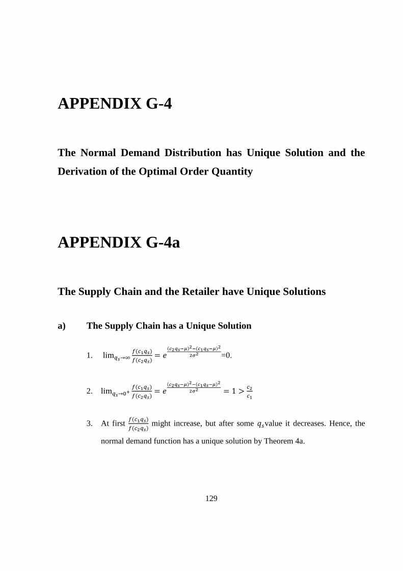
129

APPENDIX G-4

The Normal Demand Distribution has Unique Solution and the


APPENDIX G-4a



1. ( )

( )

( ) ( )

=0.

2. ( )

( )

( ) ( )

3. At first ( )

( ) might increase, but after some value it decreases. Hence, the

normal demand function has a unique solution by Theorem 4a.

130





131

APPENDIX G-4b


a) Supply Chain’s Optimal Order Quantity

We have .

/

( )

. Consider Appendix C-4b. In this problem,

we have the similar characteristics. is changed to , is changed to with

. -

, ( ) and .

/ . The optimal order quantity is:

√


Contract

-

, ( ) and .

/ , so the optimal

order quantity is :

√

132


Contract

-

, ( ) and .

/ , hence the optimal

order quantity is:

√


Contract

-

, ( ) and .

/ ; therefore the

optimal order quantity is:

√

133

APPENDIX G-5

The Calculation of the Optimal Order Quantity for the Uniform

Demand Distribution

Theorem 3 and Theorem 4 cannot be used because there is no way to satisfy the

Equation (9) to 12 with the uniform distribution. Note that there is no unique solution for the

uniform distribution. On the other hand, the order quantities below are always optimal.


By the change of necessary parameters of Appendix C-5, the optimal order quantity

is found to be .


Contract


is found to be .


Contract


is found to be .

134


Contract


is found to be .

135

APPENDIX H

Upper Bound for the Target Profit Level for the Retailer in order

for the Coordination for the Exponential, Gamma and the

Weibull Demand Distributions

APPENDIX H-1

Exponential Distribution

a) Wholesale Price Contract

When ,

and

. In order to ensure the assumptions of

the coordination, the following should be satisfied:

.

/

.

/

Hence,

136

( )

.

/

By simplifying this, we derive:

( ) .

( )

( )( )/

(

)

b) The Buy Back Contract

Assume that By applying the same procedure, we derive:

( ) .

( )

( )( )/

(

)

137

APPENDIX H-2

Gamma Distribution

a) The Wholesale Price Contract

In order to ensure the assumptions of the coordination, the following should be

satisfied:

.

/

.

/

Namely, we need to satisfy:

( ) ( ) ( )

( )

After simplification, we derive:

( )

(( )

( )( )(

)

)

(

)

Note that this is an implicit solution for because and are also functions

of .

138


Assume that The following has to be satisfied in order to ensure that the

assumptions of the coordination:

( )

(( )

( )( )(

)

)

.

/

139

APPENDIX H-3

Weibull Distribution


We need to satisfy:

.

/

.

/

In other words, the following should be satisfied:

( )

( ) ( ( ) ( ) )

where

and

when .

There is no explicit solution, but should satisfy:

( ) ( ) (

( )

( ) )


Assume that The following has to be satisfied in order to ensure that the

assumptions of the coordination:

140

( )

( )

(

(

)

( ) )

141

APPENDIX I

Upper Bound for the Target Return on Investment Level for the

Retailer in order for the Coordination for the Exponential,

Gamma and the Weibull Demand Distributions

APPENDIX I-1

The Exponential Demand


Suppose the supply chain’s optimal order quantity is When ,

( )( )

( ) and

( )

( )( ) .

We need to satisfy:

( )( )

( ) (

( )

( )( ))

After some calculations, we derive:

142

( )

( ) (

( )( )

( ) )


Assume that By applying the same procedures, we derive:

( )

( ) (

( ) ( )

( ) )

c) The Revenue Sharing Contract

Assume that

. By applying the same procedures, we derive:

( )

( ) (

( ) ( )

( ) )

143

APPENDIX I-2

Gamma Distribution


Note that when , ( )( )

( ) and

( )

( )( ) . .

/

( )

should be satisfied. Hence,

( ) .

/

should be satisfied. Therefore, ( ) .

/

.

After some calculations, we derive:

( )

( ) (

( )( )

( ) )


Assume that By applying the same procedure, we derive:

( )

( ) (

( )( )

( ) )


Assume that

. By applying the same procedure, we derive:

144

( )

( ) (

( )( )

( ) )

145

APPENDIX I-3

Weibull Distribution


Note that when , ( )( )

( ) and

( )

( )( ).

We need to satisfy .

/

( ( ) ( ) )

. Hence, (

) .

/

.

/ should be satisfied.

Note that this is all we can obtain, we can find the upper bound by trial and error.


Assume that We derive:

(

) (

)

(

)


Assume that

. We derive:

146

(

) (

)

(

)

147

APPENDIX J

Explanations of the Theorems

APPENDIX J-1

Weierstrass Theorem

The following results can be achieved by using the Weierstrass Theorem (Brinkhuis

and Tikhomirov, 2005):

A continuous function on a nonempty compact set in Rn attains its global maxima

and minima. Often we will use the following consequence. A continuous function f:Rn→R on

the whole Rn

is called coercive for minimization if:

( )

Corollary: A continuous function f:Rn→R that is coercive for minimization has a

global minimum.

148

APPENDIX J-2

Intermediate Value Theorem

A function ( ) that is continuous on a closed interval , - takes on every

value between ( ) and ( ). In other words, if is any value between ( ) and ( ), then

( ) for some in , - (Thomas et al., 2004).

supply chain coordination with different objectives · supply chain coordination with different...

Documents