supply chain design with product life cycle considerations

Supply chain design with product life cycle

considerations

Thèse à présenter pour l‘obtention du titre de :

Docteur de l‘université de Sfax, spécialité méthodes quantitatives

Docteur de l‘université d‘Artois, spécialité génie informatique et automatique

Par

Khaoula BESBES NABLI

A soutenir publiquement le 12 Décembre 2013, devant le jury composé de :

M. Abdelwaheb Rebai Professeur d‘enseignement supérieur, FSEG - Sfax Président

Mme. Taicir Moalla Loukil Professeur d‘enseignement supérieur, FSEG - Sfax Directrice de thèse

M. Gilles Goncalves Professeur des universités, Université d‘Artois Directeur de thèse

M. Hamid Allaoui Professeur des universités, Université d‘Artois Co-encadrant

M. Lyes Benyoucef Professeur des universités, Université d‘Aix-Marseille Rapporteur

M. Talel Ladhari Professeur d‘enseignement supérieur, ESSEC - Tunis Rapporteur

M. Ouajdi Koorba Professeur d‘enseignement supérieur, ISITCom -

Hammam Sousse

Membre

Année universitaire 2013 - 2014

Université d‘Artois

Ecole Doctorale des Sciences Pour l‘Ingénieur de

Lille

Faculté des Sciences Appliquées de Béthune

Université de Sfax

Ecole Doctorale des Sciences Economiques,

Gestion et Informatique de Sfax

Faculté des Sciences Economiques, Gestion et

Informatique de Sfax

Spécialité : Génie Informatique et Automatique Spécialité : Méthodes quantitatives

To my parents, to my brothers,

To my husband,

To my daughter,

To my in-laws,

To all those who believe in the richness of learning

Acknowledgements

It would not have been possible to write this doctoral thesis without the help and support of

the kind people around me, to only some of whom it is possible to give particular mention

here.

Foremost, I would like to express my deepest gratitude to my advisors Prof. Taicir Moalla

Loukil, Prof. Gilles Goncalves, and Prof Hamid Allaoui, for their continuous support of my

Ph.D study and research, for their patience, motivation, enthusiasm, and immense knowledge.

Without their encouragement and constant guidance, I could not have finished this

dissertation.

Besides my advisors, I would like to thank the rest of my thesis committee: Professors XXX,

for the time and the effort given to review and examine this dissertation.

I owe a very important debt to my husband and to my lovely daughter for their

personal support and great patience at all times. They were always there cheering

me up and stood by me through the good times and bad. Thank you for all the late

nights and early mornings, and for keeping me sane over the past few months.

Thank you for being my muse, editor, proofreader, and sounding board. But most

of all, thank you for being my best friends. I owe you everything.

Above all I would like to thank my parents, who have supported me spiritually and financially

since the beginning of my studies, and throughout my life.

I would like to show my greatest appreciation to my in-laws for their emotional

support, their encouragement, advices and for the many sacrifices they have made over a

number of years.

I would express my sincere thanks to my lovely friend Faten Toumi, for her endless support

and encouragement.

I would like to offer my special thanks to my friends and colleagues at LGI2A,

namely Vesela, Yamine, Issam, Hirsh, Samir, Hind, Andra, and Yoann, who have

taken the greater part of this PhD journey with me. I am lucky to have had a

wonderful group of friends like them. Having their support and friendship has

meant a great deal during both the good times and those when things haven’t gone

so well.

Last, but not least, I would like to thank my brothers for their love, support, and unwavering

believe in me. Without them I would not be the person I am today.

i

Contents

List of figures v

List of tables

vi

1

Introduction

1

1.1 Motivation 1

1.1 Research axes and contributions 2

2

Supply chain design with product life cycle considerations: Theoretical background and state of

the art

6

2.1 Introduction 6

2.2 Theoretical background 7

2.2.1 Supply chain decision levels 9

2.2.2 The product types, product life cycle and supply chain strategies 11

a The product types 11

b The product life cycle 11

2.2.3 The supply chain strategies 14

2.3 State of the art 19

2.3.1 The decision support for the supply chain network design 19

2.3.2 The multi-period supply chain design 20

ii

2.3.3 The multi-criteria supply chain design 21

2.3.4 The multi-objective supply chain design 23

2.3.5 The green supply chain design 24

2.3.6 The Stochastic supply chain design 27

2.4 State of the art interpretation 28

2.5 Conclusion 29

3

A multi-criteria supply chain design with product life cycle considerations

30

3.1 Introduction 30

3.2 Problem statement 31

3.3 The resolution methodology 33

3.4 Phase 1: a multi-criteria decision making model for potential actor‘s efficiency evaluation 36

3.4.1 The Analytical Hierarchical Process 38

a The AHP hierarchy 38

b The pairwise comparison 39

c The component weights 41

d The overall priority rating 43

3.4.2 The ordered Weights Averaging (OWA) operators 43

a The OWA operators: definition and priorities 44

b Fuzzy logic quantifier-guided OWA combination 46

c Inclusion of the importances in OWA operators 48

3.4.3 The AHP-OWA operator 49

3.5 Phase II: The supply chain network design 50

3.5.1 The mathematical model 52

3.5.2 The model reformulation 54

iii

3.6 Case study 56

3.7 Model limits 71

3.7.1 Review of the expected efficiency value 71

3.7.2 Review of the sets of the potential actors 71

3.7.3 The penalty method 72

3.7.4 Capacity extension 74

3.8 Conclusion 78

4

A product-driven sustainable supply chain design

80

4.1 Introduction 80

4.2 Problem definition 81

4.2.1 The advisability study: 83

4.2.2 The feasibility study 84

4.2.3 The impact assessment study 85


4.4 Numerical example 103

4.5 Sensitivity analysis 109

4.6 Conclusion and perspectives 110

5

A Supply chain design under product life cycle uncertainty

112

5.1 Introduction 112

5.2 The main topic 114

5.3 Problem statement 118

5.4 Data and uncertainty 120

5.5 The stochastic programming approach 120

5.6 Uncertainty on product life cycle 122

iv

5.6.1 The model 123

5.6.2 The mathematical formulation 125

5.7 Experimental results 127

5.8 Sensitivity analysis 130

5.8.1 Sensitivity analysis by changing the scenarios ‗probabilities 130

5.8.2 Sensitivity analysis by changing the problem size 132

5.8 Conclusion 137

6

Conclusions and perspectives

139

Bibliography

142

Appendix A 158

v

List of figures

2.1 Supply chain decision levels 10

2.2 Marketable product life cycle 13

3.1 A simple network of three-stages in supply chain network. 31


3.3 Hierarchical structure of the decision problem 39

3.4 Monotonically non-decreasing fuzzy linguistic quantifier, (Herrera et al., 2000) 47

3.5 Linguistic rating on membership function corresponding to fuzzy number 58

3.6 Sales distribution of the product in Ton 67

3.7 The deployment plan of the total supply chain 69

3.8 Fluctuations in capacities over the product life cycle 78

4.1 The Three Base Line of a sustainable supply chain, adapted from Zhong Hua Zhang

(2011)

82

4.2 Phases for the supply chain network design 89

4.3 Criteria hierarchy 90

4.4 Sales distribution of the product in Ton 108

4.5 Sensitivity by changing objective weights 110

5.1 The different PLC curves, adapted from Rink and Swan (1979)

116

vi

List of tables

2.1 The different business characteristics over the product life cycle 13

2.2 The different types of supply chains 15

2.3 The supply chain classification based on product type and product life cycle 18

2.4 Summary of research in supply chain design with product life cycle considerations 27

3.1 Scales for pairwise comparisons, adapted from Saaty(1980) 40

3.2 Random inconsistency indices (RI), adapted from Saaty(1980) 43

3.3 The core of factors on supply chain performance 58

3.4 Data collection on supply performance 59

3.5 Criteria pairwise comparison and relative weights at the introduction stage 60

3.6 Criteria pairwise comparison and relative weights at the maturity stage 60

3.7 pairwise comparison of the sub-criteria relative to the criterion ‗R&D‘ and relative

weights

61

3.8 AHP scores for the R&D criterion at the introduction stage 61

3.9 Product criteria and supply chain strategy on product life cycle 62

3.10 Potential suppliers‗ final scores for the R&D criterion at the introduction stage 63

3.11 Potential suppliers‗ efficiency scores 64

3.12 Multiple attribute matrix on production performance and efficiency scores 65

3.13 Multiple attribute matrix on distribution performance and efficiency scores 66

3.14 Optimal supply chain network for the introduction stage 70

3.15 Optimal supply chain network for the maturity stage 70

4.1 Multiple attribute matrix on supply performance and efficiency scores 105

4.2 Multiple attribute matrix on production performance and efficiency scores 106

4.3 Multiple attribute matrix on distribution performance and efficiency scores 107

vii

4.4 The optimal supply chain network 108



5.1 Data used in implementations 127

5.2 Table of results 128

5.3 Table of results for the scenarios' probabilities: (0.05, 0.85, 0.05, 0.05) 129



5.6 Table of results for 6 suppliers- 6 producers – 6 distributors 131






A.1 Pairwise comparison of the sub-criteria relative to the criterion ‗Cost‗ and relative

weights 160

A.2 AHP scores for the cost criterion at the introduction stage 160

A.3 Pairwise comparison of the sub-criteria relative to the criterion ‗Quality‗ and relative

weights 161

A.4 AHP scores for the criterion ‗Quality‗ at the introduction stage 161

A.5 Pairwise comparison of the sub-criteria relative to the criterion ‗service‗ and relative

weights 161

A.6 AHP scores for the criterion ‗Service‗ at the introduction stage 162

A.7 Pairwise comparison of the sub-criteria relative to the criterion ‗Response‗ and relative

weights 162

A.8 AHP scores for the criterion ‗Response‗ at the introduction stage 162

A.9 OWA weights for the criterion ‗R&D‗ in the introduction stage 163

A.10 OWA weights for the criterion ‗Cost‗ in the introduction stage 164

A.11 OWA weights for the criterion ‗Quality‗ in the introduction stage 165

A.12 OWA weights for the criterion ‗Service‗ in the introduction stage 166

A.13 OWA weights for the criterion ‗Response‗ in the introduction stage 167

A.14 The AHP-OWA scores for the different criteria at the introduction stage 168

A.15 The aggregation weights 169

A.16 The final efficiency scores for the suppliers at the introduction stage 169

Abstract

Our research addresses the problem of designing a multi-level supply chain, while taking into

consideration the product life cycle. By product life cycle, we mean the succession of the four

marketing stages that a product goes through since its introduction to the market and until it

will be removed from. All products have a life cycle. Generally this life cycle can be

classified into four discrete stages: introduction, growth, maturity and decline.

Depending on the product life cycle phases, and based on a thorough analysis of the different

supply chain potential actors, this study aims to establish mathematical models to design an

efficient supply chain network.

Three main models have been developed in this thesis.

The first proposed model aims to design a product-driven supply chain with a minimal total

cost, taking into consideration the evaluation of the different potential actors effectiveness,

according to several criteria (cost, quality, innovation, quality service, timely delivery ...).

A second model was developed to design of a sustainable supply chain network, taking into

account the product life cycle. In this model, three different objectives were simultaneously

considered, namely, an economic objective, an environmental objective and a social objective.

In the two previous models, we have assumed that the product has a classical life cycle.

However, in the reality this is not always the case. Indeed, some products have very atypical

life cycles, whose curves are very different from the classical one.

To tackle this problem, in the third part of this thesis, we propose a stochastic model to

design a robust supply chain network, taking into account the different product life cycle

scenarios.

Résumé

Notre travail de recherche traite la problématique de la conception d‘une chaîne

logistique multi-niveaux tout en tenant compte du cycle de vie du produit. Par cycle de vie du

produit, nous entendons la succession des quatre phases de commercialisation que traverse

généralement un produit à travers le temps, à savoir : l‘introduction, la croissance, la maturité

et le déclin. L‘objectif est de mette en place un modèle mathématique qui soit fondé sur une

analyse approfondie des différents acteurs de la chaîne, selon la phase du cycle de vie du

produit.

Trois principaux modèles ont été développés dans cette thèse. Chacun fait l‘objet d‘un

chapitre à part entière.

Le premier modèle développé vise à concevoir une chaîne logistique de coût

minimum, tout en prenant en considération l‘efficacité des différents acteurs potentiels

calculée selon plusieurs critères (coût, qualité, innovation, qualité du service, délais de

livraisons, …), ainsi que sa variation au cours du cycle de vie du produit.

Un deuxième modèle a été mis en place pour la conception d‘une chaîne logistique

durable, tout en prenant en considération le cycle de vie du produit. Dans ce modèle, trois

objectifs différents ont été pris en compte à la fois, à savoir, un objectif économique, un

objectif environnemental et un objectif social.

Dans les deux premiers modèles, nous avons supposé que le produit aura un cycle de

vie classique. Cependant, dans la réalité, ceci n‘est pas toujours le cas. En effet, quelques

produits connaissent des cycles de vie très atypiques et donc très éloignés de la courbe d‘un

cycle de vie théorique.

Pour ce faire, un troisième modèle stochastique a été proposé pour la conception

d‘une chaîne logistique robuste, tenant compte des différents scénarios du cycle de vie du

produit.

1

1.1 Motivation

Globalization has increased the complexity of supply chains with the involvement of more

stakeholders, facilities, and technologies. Therefore, many new challenges and complexities

have emerged in the field of supply chain management.

Indeed, global competition has imposed a tremendous pressure on product and service

providers to transform and improve their operations and practices. Companies are responding

to this pressure by reengineering and streamlining their operations to better serve their

customers. More specifically, firms are involved in improving the performance of their supply

chains through various strategic and operational tools. One of the strategies utilized by

companies is to concentrate on their core competencies in the chain value and outsource of the

other functions. Actually, firms are indulged in strategic organizational networks such as

network organizations, virtual corporations, and value-added partnerships. However, the

success of supply chain networks depends ,to a large extent, on how effectively they are

designed and operated.

These supply chain networks are considered as a solution to effectively meet the customer's

requirements such as low costs, a high product variety, high quality, and short lead times

CHAPTER 1

Introduction

2

(Busby and Fan, 1993; Byrne, 1993; Goldman, 1994; Iacocca Institute, 1991; Johnston and

Lawrence, 1988; Snow et al., 1992).

Referring to marketing the literature, we note that this performance is directly related to the

life cycle of the product. Indeed, the product life cycle could direct the supply chain to the

appropriate market strategy.

Similarly, it should be noted that the consumer's requirements are closely linked to the

product life cycle and their relative importance differs from one stage to another; for instance,

availability and technology are needed at the ‗‗introduction‘‘ phase, and cost, quality and

speed are needed at the ‗‗maturity‘‘ phase.

Facing this problem, the whole company should carefully manage the product life cycle, and

the supply chain actors‘ mechanism should also be matched up concurrently.

Nokia, the Finnish mobile phone manufacturer for example, manufactures the early series of

its products in Finland at a product launch, and once established, will hand a volume

production to contract manufacturers who are located in the Baltic and in China, and at the

end of the life span (in some cases) even taking the production back in-house as they become

close to withdrawing the product from the market.

The main concept that we focus on ,in this thesis, is the consideration of the product life cycle

in the supply chain network design.

1.2 Research axes and contributions

This introductory Chapter is followed by the theoretical background and the state of art in

Chapter 2, which is a review of the Supply Chain Network Design approaches and resolution

methods. Among other things, we recall the different decision levels in the Supply Chain

(strategic, tactical and operational level), the supply chain network structure (single/multiple

layer(s), single/multiple product(s), single/multiple period(s), single/multiple objective (s),

3

single/multiple modality, deterministic/stochastic parameters) and existing deterministic

SCND models and SCND models under uncertainty.

For an effective supply chain, the assessment of actors and the selection process are essential

for improving the performance of a focal company and its supply chains. An investigation is

made, in chapter 3, to develop a selection procedure of supply chain actors by considering

different selection criteria and different product life cycle phases.

An attempt is made to ensure that the evaluation results satisfy the current product

competition strategies, and also improve the effectiveness and efficiency of the entire supply

chain. The resolution procedure is made up of two phases. In the first phase, a multi-criteria

decision making problem is proposed for the supply chain actors‘ evaluation.

A combination between the Analytical Hierarchical Process (AHP) and the Fuzzy Linguistic

Quantifier Guided Order-Weighted Aggregation (FLQG-OWA) operator is used to satisfy the

enterprise product development strategy based on different phases of the product life cycle.

The second phase looks for the optimal supply chain design to satisfy the customer's

demands and economic criteria using a mixed integer linear programming model.

As supply chains have grown tremendously in recent years, focusing only on the economic

performance to optimize the costs or returns of the investments (ROIs), became not sufficient

to sustain the development of supply chain operations. Indeed, the impact of different

activities that are involved in supply chains, such as the process of manufacturing,

warehousing, distributing etc. on the environment and social life of city residents cannot be

ignored.

Correspondingly, the concepts of green supply chain management and sustainable supply

chain management have emerged to emphasize the importance of implementing

4

environmental and social concerns simultaneously with economical factors in supply chain

planning.

In chapter 4 of this thesis, we study the problem of designing sustainable supply chain

networks. However, few studies endeavor to optimize economic returns, environmental

concerns, and the social performance, all together for supply chains. The challenging issues

are how to achieve a certain balance among the business goals, social concerns, and the

environmental impacts of different activities in supply chains. This chapter focuses on the

problem of designing sustainable supply chain networks and taking into consideration the

triple bottom lines of maximizing economic returns, minimizing environmental impacts, and

maximizing the social performance for the supply chains. We use the Weighted Goal

Programming (WGP) approach seeking to reach the three set goals.

Up to this level of the thesis, we have only considered the classical product life cycle curve.

However, numerous marketing-oriented articles have discussed the product life cycle theory,

and they all reached an agreement on the fact that there may be different scenarios of life

cycle curves, that could be different from the classical ones.

Indeed, the classical PLC shape that we have used in the previous chapters, has been only one

of 12 types of PLC patterns discovered by the investigators.

Theoretically, product sales follow a bell curve, and the product life cycle should begin with

the introductory stage, then growth, maturity and finally the decline stage.

Although this scenario remains the most classical, in reality, products could have been very

atypical life cycle curves and so, very far from the theoretical life cycle curve.

As uncertainty is one of the characteristics of the product-driven supply chain networks, the

strategic phase has to take uncertain information into account.

5

Certainly, the supply chain structure must be very robust to deal with the unpredictable

market demand, the uncompromising levels of competition, and the different product life

cycle patterns.

In chapter 5 of the thesis, we present a based stochastic programming method that seeks a

solution which is appropriately balanced among some alternative product life cycle scenarios,

as identified by field experts. We apply the stochastic models to a representative real case

study. The interpretation of the results is meant to grant more insight to decision-making

under the uncertainty of the supply chain design.

Finally, chapter 6 concludes the research findings and the activities undertaken throughout the

thesis.

6

2.1 Introduction

This chapter is devoted to introduce general supply chain design problems and more

specifically the particular supply chain design problem with product life cycle considerations.

We present the basic concepts that are necessary to understand the different issues and

concepts discussed in this thesis.

We first present the concept of the supply chain, the different supply chain decision levels,

and some supply chain strategies.

Then, we are particularly interested in the supply chain design problem with product life cycle

considerations. We introduce the different product types, define the product life cycle

concept, and present some supply chain design strategies as proposed in the literature dealing

with linking the supply chain design to the product life cycle, according to the product type.

After, a non-exhaustive review of various supply chain design problems proposed in the

literature was illustrated, as well as the different resolution methods proposed to solve them.

CHAPTER 2

Supply chain design with product life cycle

considerations:

Theoretical background and state of the art

7

Finally, we present the few studies in the literature that consider the product life cycle in the

supply chain design network problem.

2.2 Theoretical background

The past decade has witnessed an increasing recognition of the importance of the supply chain

management. In industry, the rapid growth of supply chain software companies testifies to the

significance that businesses place on the efficient management of their supply chains.

Research in this area has become a key focus of the operations of the management academic

community in recent years.

The current research on supply chain management has covered conceptual issues and

managerial themes (Cox and Lamming, 1997), frameworks for strategy implementation

(Harland, 1996), social aspects of supply chain management (Price, 1996), coordinated

management of the supply chain (Thomas and Griffin, 1996), the application of inter-

organizational information systems in the supply chain (Holland, 1995), design and analysis

of supply chain models (Beamon, 1998), etc.

But what exactly is supply chain and supply chain management?

Numerous definitions of a supply chain exist in the literature.

According to Beamon (1998), a supply chain is ‗‗an integrated process wherein a number of

various business entities; namely suppliers, manufacturers, distributors, and retailers; work

together in an effort to: (1) acquire raw materials, (2) convert these raw materials into

specified final products, and (3) deliver these final products to retailers‘‘ .This chain is

traditionally characterized by the flow of materials and information both within and between

business entities.

8

Mentzer et al. (2001) defined the supply chain as a set of organizations directly linked by one

or more upstream and downstream flows of products, services, finances, and information from

a source to a customer.

Another definition is given by Simchi-Levi et al. (2003), who state that supply chains are

flexible, dynamic and complex networks of organizations.

A customer focused definition is given by Hines (2004) "Supply chain strategies require a

total systems's view of the linkages in the chain that work together efficiently to create

customer satisfaction at the end point of delivery to the consumer. As a consequence, costs

must be lowered throughout the chain by driving out unnecessary costs and focusing attention

on adding value. Throughout efficiency must be increased, bottlenecks removed and

performance measurement must focus on total systems efficiency and equitable reward

distribution to those in the supply chain adding value. The supply chain system must be

responsive to customer requirements".

According to the Council of Supply Chain Management Professionals , supply chain

management encompasses the planning and management of all activities involved in sourcing,

procurement, conversion, and logistics' management. It also includes the crucial components

of coordination and collaboration with channel partners, who can be suppliers, intermediaries,

third-party service providers, and customers. In essence, supply chain management integrates

both supply and demand management within and across companies.

This definition leads to several observations. First, supply chain management takes into

consideration every facility that has an impact on cost and plays a role in making the product

conform to the customer's requirements: from supplier and manufacturing facilities , through

warehouses and distribution centers to retailers and stores. Indeed, in some supply chain

analyses, it is necessary to account for the suppliers‘ suppliers and the customers‘ customers

because they have an impact on the supply chain performance.

http://en.wikipedia.org/wiki/Council_of_Supply_Chain_Management_Professionals

http://en.wikipedia.org/wiki/Sourcing

http://en.wikipedia.org/wiki/Procurement

http://en.wikipedia.org/wiki/Logistics_management

http://en.wikipedia.org/wiki/Channel_partner

http://en.wikipedia.org/wiki/Suppliers

http://en.wikipedia.org/wiki/Intermediaries

http://en.wikipedia.org/wiki/Customers

http://en.wikipedia.org/wiki/Supply_and_demand

9

Second, the objective of supply chain management is to be efficient and cost-effective across

the entire system; total system wide costs, from transportation and distribution to inventories

of raw materials, work in process, and finished goods, are to be minimized. Thus, the

emphasis is not on simply minimizing transportation cost or reducing inventories but, rather,

on taking a system's approach to supply chain management. Finally, because supply chain

management revolves around an efficient integration of suppliers, manufacturers, warehouses,

and stores, it encompasses the firm‘s activities at many levels, from the strategic level through

the tactical to the operational one.

2.2.1 Supply chain decision levels

Supply chain management decisions are often said to belong to one of three levels;

the strategic, the tactical, or the operational level.

At the strategic level, company management makes high level strategic supply chain decisions

that are relevant to the whole organization. The decisions that are made with regards to the

supply chain should reflect the overall corporate strategy that the organization is following.

The strategic supply chain processes that management has to decide upon whether or not it

will cover the breadth of the supply chain. These processes include product development,

customers, manufacturing, sellers and logistics.

Tactical supply chain decisions focus on adopting measures that will produce cost benefits for

a company. Tactical decisions are made within the constraints of the overarching strategic

supply chain decisions made by the company management.

Operational supply chain decisions can be made hundreds of times each day in a company.

These are the decisions that are made at business locations that affect how products are

developed, sold, moved and manufactured. Operational decisions are made with an awareness

of the strategic and tactical decisions that have been adopted within a company. These higher

10

level decisions are made to create a framework within the company‘s supply chain and to

operate the best competitive advantage. The day to day operational supply chain decisions

ensure that the products efficiently move along the supply chain achieving as such the

maximum cost benefit.

Figure 2.1: Supply chain decision levels

The effective supply chain design calls for robust analytical models and design tools. Previous

works in this area are mostly operation research oriented without taking into account the

manufacturing aspects.

In the last decade, researchers began to realize that the decision and integration effort in

supply chain design should be driven by the manufactured product, specifically, product

characteristics and product life cycle.

This problem has two main aspects: the importance of the product life cycle in the supply

chain strategy, and the decision support models for the supply chain network design.

Consequently, we review the relevant the literature pertaining to these two themes.

11

2.2.2 The product types, product life cycle and supply chain strategies

a. The product types

Generally, products can be categorized into three types, namely, functional, innovative, and

hybrid (Huang et al., 2002).

Functional products‘ demand can be forecast quite accurately and their market share remains

fairly constant. They enjoy the life cycle with a superficial design modification leading to

different product types.

Innovative products are new products developed by organizations to capture a wider share of

the market. They are significantly different from the available product types and are more

adapted to the customer requirements (mass customization). They, at times, represent a

breakthrough at the level of product design. Innovative products are the result of customers'

designs, which indicate their ever-changing requirements.

Hybrid products can consist of either (a) different combinations of functional components, or

(b) a mixture of functional and innovative components.

b. The product life cycle

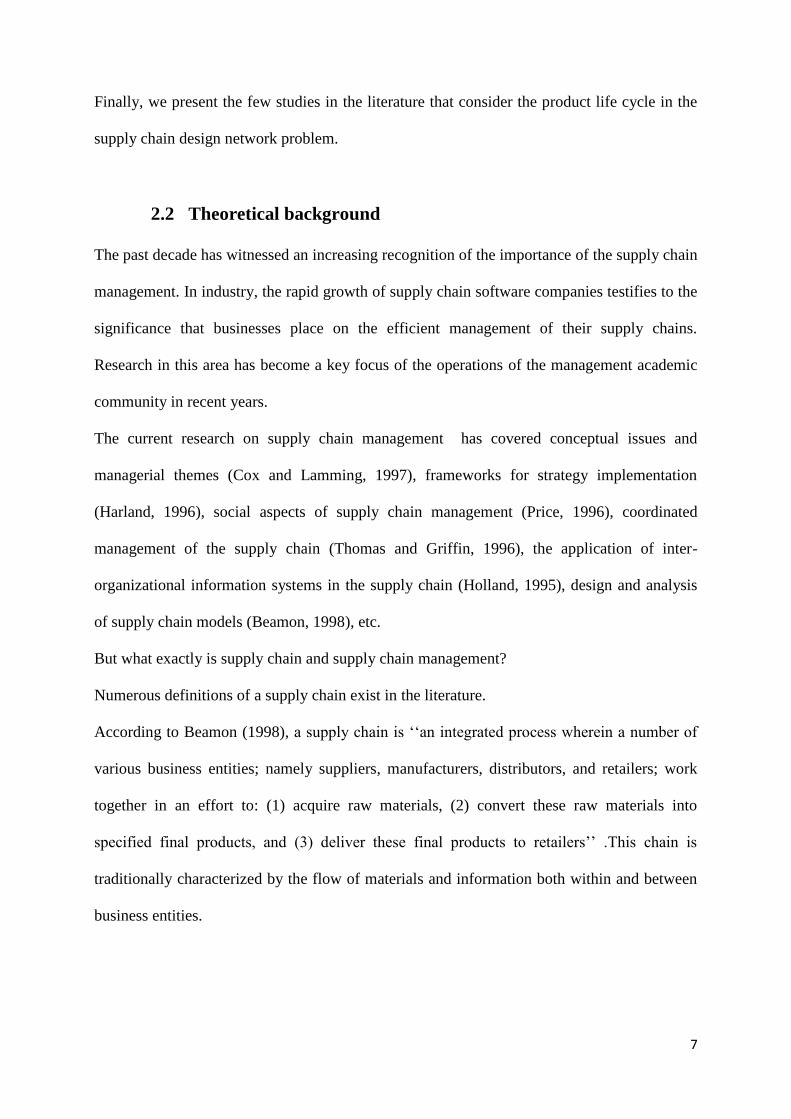
All products have a life cycle, typically depicted as a curve of unit sales for a product

category over time (Wiersema, 1982), which can be classified into four discrete stages:

introduction, growth, maturity and decline.

When the product is introduced, sales will be low until customers become aware of the

product and its benefits. The distribution is selective and scattered as the firm starts the

implementation of the distribution plan. During the introductory stage, the firm is likely to

incur additional costs associated with the initial distribution of the product. These higher costs

coupled with a low sales' volume usually make the introduction stage a period of negative

profits.

12

After, sales' volume grows as the customers become more aware of the product and its

benefits and additional market segments are targeted. An improvement of the product quality

may be considered. The distribution becomes more intensive and trade discounts are minimal

if wholesalers show a strong interest in the product. The growth stage is a period of a rapid

revenue growth.

The maturity stage is the most profitable. Into this stage, sales' volume continues to increase,

but at a slower rate. New distribution channels are selected in order to avoid losing shelf

space. The primary goal during the maturity stage is to maintain market share and extend the

product life cycle.

After the period of maturity, eventual sales come to decline as the market becomes saturated,

the product becomes technologically obsolete, or customers' tastes change. In this decline

stage, distribution becomes more selective and channels that are no longer profitable are

phased out.

Table 2.1 summarizes the different business characteristics over the product life cycle.

If a curve is drawn showing the product sales volume, over a fixed time horizon H, it may

take one of many different shapes, the most classical among them is shown in figure 2.2.

13

Table 2.1: the different business characteristics over the product life cycle

Stage Introduction Growth Maturity Decline

Market growth rate Slight Very large Moderate to nil Negative

Technological change

in product design Very great Great Moderate to slight slight

Key business

opportunity

Capturing market

leadership

Capturing

market share

Capturing market

volume

Capturing

market legacy

demand

Key business risk Investing in a wrong

technology/product

Failing to

manage ramp up

Price ware/price

erosion

Obsolete

stocks

Figure 2.2: Marketable product life cycle

14

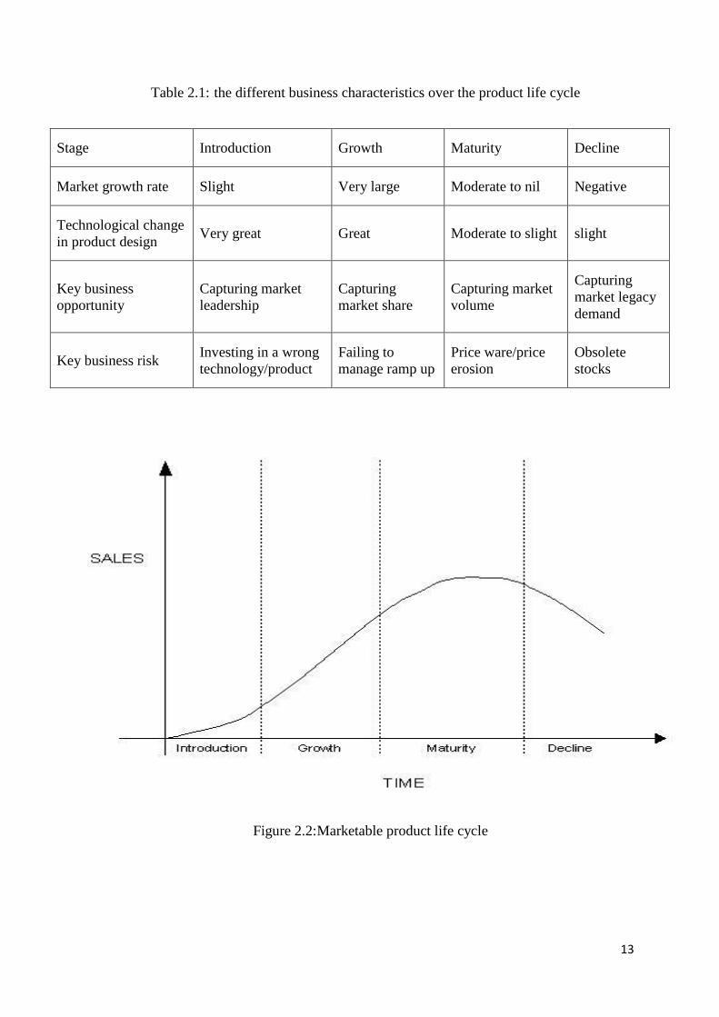
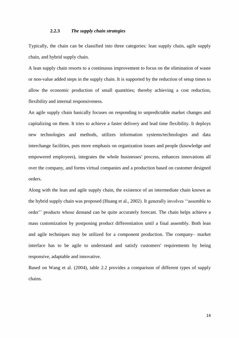
2.2.3 The supply chain strategies

Typically, the chain can be classified into three categories: lean supply chain, agile supply

chain, and hybrid supply chain.

A lean supply chain resorts to a continuous improvement to focus on the elimination of waste

or non-value added steps in the supply chain. It is supported by the reduction of setup times to

allow the economic production of small quantities; thereby achieving a cost reduction,

flexibility and internal responsiveness.

An agile supply chain basically focuses on responding to unpredictable market changes and

capitalizing on them. It tries to achieve a faster delivery and lead time flexibility. It deploys

new technologies and methods, utilizes information systems/technologies and data

interchange facilities, puts more emphasis on organization issues and people (knowledge and

empowered employees), integrates the whole businesses' process, enhances innovations all

over the company, and forms virtual companies and a production based on customer designed

orders.

Along with the lean and agile supply chain, the existence of an intermediate chain known as

the hybrid supply chain was proposed (Huang et al., 2002). It generally involves ‗‗assemble to

order‘‘ products whose demand can be quite accurately forecast. The chain helps achieve a

mass customization by postponing product differentiation until a final assembly. Both lean

and agile techniques may be utilized for a component production. The company– market

interface has to be agile to understand and satisfy customers' requirements by being

responsive, adaptable and innovative.

Based on Wang et al. (2004), table 2.2 provides a comparison of different types of supply

chains.

15

Table 2.2: the different types of supply chains

Category Lean supply chain Agile supply chain

Hybrid supply chain

Purpose

Focus on cost reduction and flexibility

for already available products.

Primarily aims at cost cutting,

flexibility and incremental

improvements in products.

Aims to produce in any volume and

deliver to a wide variety of market

niches simultaneously.

Provides customized products

at short lead times (responsiveness)

by reducing the cost of variation.

Employ lean production methods

manufacturing. Interfaces with the

market to understand customer

requirements.

Length of product life

cycle

Standard products have

relatively long life cycle times

(>2 years ).

Innovative products have short

life cycle times (3 months–1

year).

Involved the production of

‗‗assemble to order‘‘ products,

which stay in the maturity phase of the

life cycle for a long time.

Demand patterns

Demand can be accurately

forecasted and average margin

of forecasting error tends to be

low, roughly 10%

Demand are unpredictable with

forecasting errors exceeding

50%.

The average product demand can be

accurately forecasted. Component level

forecasting may involve larger errors.

16

Approach to choosing

suppliers

Supplier attributes involve low

cost and high quality.

Supplier attributes involve

speed, flexibility, and quality.

Supplier attributes involve low cost

and high quality, along with the

capability for speed and flexibility, as

and when required.

Production planning

Works on confirmed orders and

reliable forecasts.

Has the ability to respond

quickly to varying customer

needs (mass customization).

Works on confirmed orders and

reliable forecasts with some ability to

achieve some produce variety.

Product design strategy

Maximize performance and

minimize cost.

Design products to meet

individual customer needs.

Use modular design in order to

postpone product differentiation for as

long as possible.

Approach to

manufacturing

Advocates lean manufacturing

techniques.

Advocates agile manufacturing

techniques, which is an

extension of lean manufacturing.

Employs lean and agile

manufacturing techniques

Manufacturing focus

Maintain high average

utilization rate.

Deploy excess buffer capacity to

ensure that raw material/

components are available to

manufacture the innovative

products according to market

requirements.

Combination of lean and agile supply

chain

depending on components

17

Inventory strategy

Generates high turns and

minimizes inventory throughout

the chain.

Make in response to customer

demand.

Postpone product differentiation and

minimize functional components

inventory.

Lead time focus

Shorten lead-time as long as it

does not increase cost.

Invest aggressively in ways to

reduce lead times.

Similar to the lean supply chain at

component level (shorten lead-time but

not at the expense of cost). At product

level, to accommodate customer

requirements.

Human resources

Empowered individuals working in

teams in their functional departments.

Involves decentralized decision

making. Empowered individuals

working in cross-functional teams,

which may be across company

borders too.

Empowered individuals working in

teams in their functional departments.

18

Table 2.3: the supply chain classification based on product type and product life

cycle

The discussions in marketing and logistic the literature universally conclude that the product

life cycle stages have a great impact on the appropriate supply chain design. Consequently,

depending on the product life cycle stage, a firm should select its effective supply chain

partners and dynamically match the supply chain strategies to satisfy the product requirements

across multiple criteria and to maximize competitiveness over time. Indeed, the competitive

criteria generally differ depending on the product type and the product life cycle phase. Based

on Wang et al. (2004), table 2.3 summarizes the supply chain classification based on product

type and product life cycle.

The consideration of the product life cycle in the design of the supply chain has started to

receive more interest in the last decade. However, there are still gaps to fill. Indeed, it should

be noted that all existing papers dealing with this subject in the literature, focus only on one

level, namely the suppliers.

Product life cycle

Product type

Functional Innovative Hybrid

Introduction Lean Supply chain Agile Supply chain Hybrid Supply chain

Growth Lean Supply chain Agile Supply chain Hybrid Supply chain

Maturity Lean Supply chain Hybrid/Lean Supply chain Hybrid Supply chain

Decline Lean Supply chain Hybrid/Lean Supply chain Hybrid Supply chain

19

In the following, we classify the research on supply chain design with product life cycle

consideration into four major categories and list representative publications in table 2.4. From

this table, we can remark that, in the literature, many papers have only suggested marketing

strategies to link the supply chain design with the product life cycle.

Also, only few researchers have treated the problem as an optimization problem, while these

decision-making processes should be guided by a comprehensive set of performance metrics.

Another main point to notice is that, even the few papers that have dealt with the problem as

an optimization one, have taken into consideration only a single supply chain level and only a

single product life cycle period.

2.3 State of the art

2.3.1 The decision support models for the supply chain network design

The literature about the supply chain design is very rich in mathematical models addressing

different issues referring to this problem, but despite the success in resolving these supply

chain design problems, the existing models and resolution procedures are more often confined

to a single period, and are not designed to handle the design of a multi-level supply chain

taking into account the different phases of a product life cycle.

Dolgui et al. (2005) presented a set of modelling techniques taking into account the enterprise

integration problem, the knowledge management in the SME networks, and the human

resources in business process engineering. They considered all the stages of product life cycle

in an integrated approach, from the product/process design to the customer delivering.

Thomas et al. (2008) proposed a special procedure based on mathematical programming

modelling to obtain a stable Master Production Schedules (MPS) on the basis of a stable and

robust Sales and Operations Planning (SOP).

20

Dolgui and Proth (2012) considered how modern production and operations management

techniques can respond to the pressures of the competitive global marketplace. It presents a

comprehensive analysis of concepts and models related to outsourcing, dynamic pricing,

inventory management, RFID, and flexible and re-configurable manufacturing systems, as

well as real-time assignment and scheduling processes.

2.3.2 The multi-period supply chain design

Arntzen et al. (1995) developed a model for a global multi-period supply chain system,

incorporating a bill of material constraints. The model contains several international features

such as duty relief and drawback. The authors reported the solutions of several real life cases

by employing non- traditional solution methods, such as elastic constraints, row factorization,

cascaded problem solution, and constraint-branching enumeration.

Hinojosa et al. (2000) addressed the use of a mixed integer programming for solving a multi-

period two- echelon multi-commodity capacitated location problem. They proposed a

lagrangean relaxation to solve the problem, together with a heuristic procedure that constructs

feasible solutions of the original problem from the solutions at the lower bounds obtained by

the relaxed problems.

Canel et al. (2001) developed an algorithm to solve the capacitated, multi-commodity,

dynamic, and multi-stage facility location problem. Their algorithm consisted of two parts: in

the first part, a branch and bound procedure is used to generate several candidate solutions for

each period, and then a dynamic programming is used to find an optimal sequence of

configurations over the multi-period planning horizon.

Yildirim et al. (2005) studied a dynamic planning and sourcing problem with service level

constraints. Specifically, the manufacturer must decide how much to produce, where to

produce, when to produce, how much inventory to carry, etc., in order to fulfill random

21

customer demands in each period. They formulated the problem as a multi-period stochastic

programming problem, where service level constraints appear in the form of chance

constraints (Birge and Louveaux, 1997).

2.3.3 The multi-criteria supply chain design

The manufacturing strategy the literature suggests five categories of competitive priorities:

cost, quality, delivery, flexibility, and innovation (Hayes & Wheelwright, 1979). Strategic

sourcing recognizes that suppliers have a strategic role and that an effective configuration of

the supply base and development of the appropriate buyer– supplier relationships can provide

access to resources for achieving competitive priorities (Carr & Pearson, 1999; Narasimhan &

Das, 1999; Krause, Scannell, & Calantone, 2000). Consequently, the evaluation and selection

of the suppliers according to the buyer‘s changing priorities is important in the strategic

sourcing.

The product life cycle offers a framework to plan and examine the sourcing strategy of a firm

(Birou et al., 1998; Rink & Dodge, 1980). The product life cycle of both the procured

products and end products, manufactured by a firm, would affect the sourcing context and

should, therefore, be considered in the analysis. Based on the empirical research, Rink and

Fox (1999) developed a PLC-oriented procurement framework which suggests that the

sourcing strategy for the components that strongly influence sales of end products should be

governed by the competitive priorities of the end products. Their study suggests that a buying

firm‘s relative priority for cost increases from introduction to maturity stage as the end

product becomes increasingly standard.

When the product life cycle of procured components is strongly linked to that of the end

products (Tibben-Lembke, 2002), it follows that the relative importance of cost for the

procured components also increases over time as they become increasingly standardized.

22

Consequently, the buyer emphasizes the cost toward the later stages of a component‘s product

life cycle (Reed, 2002).

In some real-life situations, decision makers may not possess a precise or sufficient level of

knowledge of the problem, or are unable to discriminate explicitly the degree to which a

criterion is more important than another or one alternative is better than other. In such cases, it

is very suitable to express the decision maker‘s preference values with the use of a linguistic

variable rather than exact numerical values (Bordogna et al.1997; Kacprzyk, 1986; Zadeh,

1975).

Many techniques were used to tackle the multi-criteria decision making problems using

linguistic terms. Among these methods, we can cite the Analytical Hierarchical Process

(AHP).

This method provides a framework to cope with multiple criteria situations, involving

intuitive, rational, qualitative, and quantitative aspects (Khurrum et al.(2002)).

Ghodsypour and O‘Brien (1998) solved a supplier selection problem using a hybrid approach

involving AHP and linear programming.

Wang, et al. (2004) applied the AHP method to choose a strategy from the agile/lean supply

chain. Further, they used the Pre-emptive Goal Programming (PGP) to obtain the optimal

order quantity from the suppliers. Tuzkaya et al. (2008) included qualitative and quantitative

criteria (benefits, opportunities, costs and risks), to assess and select undesirable facility

locations. Further, Kumar et al. (2008) solved a supplier selection problem using AHP and a

fuzzy linear programming. Ku et al. (2010) and Lee et al. (2006b) used fuzzy AHP and fuzzy

goal for the supplier selection. In their model, the fuzzy AHP was first applied to calculate

the weights of the criteria. These weights were subsequently used in a fuzzy goal

programming to select the supplier.

23

Furthermore, many aggregation operators have been developed to aggregate a linguistic

preference information during the aggregation phase, such as the linguistic Ordered Weighted

Averaging operators OWA.

Chang et al. (2006) proposed a fuzzy multiple attribute decision making method based on the

fuzzy linguistic quantifier. They attempted to ensure that the evaluation results satisfy the

current product competition strategies, and improve the effectiveness and efficiency of the

entire supply chain. They applied the fuzzy concept to both the ordinal and cardinal pieces of

information, and used the Fuzzy Linguistic Quantifier Guided Order-Weighted Aggregation

(FLQG-OWA) operator to satisfy the enterprise product development strategy based on

different phases of the product life cycle.

This operator allows the aggregation of different amounts and numbers of sets into a single

final evaluation value, in accordance to the distinct fuzzy linguistics. The fuzzy quantifier acts

as a medium for aggregating the evaluation values among different attributes, which

represented the outcome of evaluation for each supply chain actor by decision makers.

Wang et al. (2009) presented a further research that is deeper into the concept introduced in

Chang et al. ( 2006), using a multi-granularity linguistic variable and numerical ration scale to

represent the overall supply performance. They resolved the measurement complexity by

unifying the derived information, and constructed a fuzzy preference to adjust the consistent

direction and transform information into a fuzzy relationship. Finally, the fuzzy linguistic

quantifier guided ordered weighted aggregation (FLQG-OWA) operator with a maximal

entropy was computed and aggregated with all indicators to meet the current policy of the

focal company.

Besbes et al. (2012) presented a multi-phase mathematical programming approach for

effective supply chain design with product life cycle considerations. The methodology

24

proposed develops and applies a combination of multi-criteria decision making models, based

on aggregation concepts, and linear and integer programming methods.

Singh and Benyoucef (2013) presented a fuzzy TOPSIS and soft consensus based group

decision making methodology to solve the multi-criteria decision making problems in supply

chain coordination, i.e., selection problems. The methodology is proposed to improve the

coordination in decentralized supply chains, i.e., supply chains that comprise several

independent, legally separated entities with their own decision authorities.

Lajili et al. (2013) considered the multi-criteria inventory classification problem. They

proposed a new classification algorithm referred to as Constructive Order Classification

Algorithm (COCA). This algorithm is based on some simple priority rules and aims to

standardize the classification and provide relative stability in the classification through a

consensus process.

2.3.4 The multi-objective supply chain design

In spite of the complexity and economic importance of the supply chain actors‘ selection,

relatively less attention has been paid, in the literature, to the application of mathematical

programming methods for the actors‘ selection and the supply chain network design.

The initial research in this area mainly dealt with single-objective and single-product supplier

selection problems, and subsequent studies increasingly focused on multi-criteria, multi-

objective, multi-product cases.

Several studies have applied the multi-objective programming MOP approach for supplier-

selection problems (e.g., Akinc, 1993; Weber & Ellram, 1993; Weber, Current, & Desai,

2000). These models allow the allocation of orders to suppliers who satisfy the minimum

performance criteria across multiple dimensions, that are; delivery, quality, and other factors.

25

Roghanian et al. (2007) considered a probabilistic bi-level linear multi-objective

programming problem and its application in enterprise-wide supply chain planning problem,

where market demand and warehouse capacity are random variables.

Alcada-Almeida et al. (2009) proposed a multi-objective programming approach to identify

locations and capacities of hazardous material incineration facilities and balance the social,

economic, and environmental impacts.

Benyoucef and Xie (2011) addressed the design of supply chain networks including both

network configuration and related operational decisions such as order splitting, transportation

allocation and inventory control. The goal is to achieve the best compromise between cost and

customer service level. They proposed an optimisation methodology that combines a multi-

objective genetic algorithm (MOGA) and simulation to optimise not only the structure of the

network but also its operation strategies and related control parameters. They also developed a

flexible simulation framework to enable the automatic simulation of the supply chain network

with all possible configurations and all possible control strategies.

2.3.5 The green supply chain design

Green supply chains, or environmentally conscious supply chains, involve the design and

implementation of supply chains that incur minimal environmental impact (Sarkis, 2006).

Environmental awareness and legislation have successfully pushed companies to aim at

manufacturing greener products that would have less impact on the environment through all

the stages of their manufacturing and distribution (Azzone and Noci,1996). Reducing the

supply chain‘s emissions has become a necessary obligation, and the trade-offs in the supply

chain are no longer just about cost, service and quality, but cost, service, quality and carbon,

(Butner et al. 2008).

26

Ramudhin et al. (2008) introduced a Mixed Integer Linear Program (MILP) formulation of

the green supply chain design network problem. Their model focuses on the impact of

transportation, subcontracting, and production activities on the design of a green supply chain.

Wang et al. (2011) proposed a multi-objective optimization model that captures the trade-off

between the total cost and the environmental influence.

Abdallah et al. (2012) developed a MILP for the carbon-sensitive supply chain that minimizes

the emissions throughout the supply chain by taking into consideration the green procurement.

Elhedhli and Merrick (2012) developed a green supply chain design model that incorporates

the cost of carbon emissions into the objective function. The goal of the model is to

simultaneously minimize the logistics' costs and the environmental CO2 emissions cost by

strategically locating warehouses within the distribution network.

Jaegler and Burlat (2012) focused on CO2 emissions along supply chains, from freight energy

use to inventories storage. Their purpose was to compare levels of CO2 emitted for differing

configurations of different scenarios.

Chaabane et al. (2012) presented a mixed-integer linear programming based framework for a

sustainable supply chain design with Life Cycle Assessment (LCA) considerations. The LCA

is a theory that is very different from the PLC. The LCA is the process that evaluates the

environmental impacts associated with a product, process or activity. It identifies and

quantifies the energy and materials used and the waste released into the environment, and

evaluates and implements the possible opportunities for environmental improvements. The

assessment covers the entire life cycle of the product, process or activity, including extracting

and processing raw materials, manufacturing, transportation and distribution, reuse and

maintenance, recycling and final disposal. Besbes et al. (2013) presented a two-phase

mathematical programming approach for effective supply chain design with a total cost

minimization, while considering environmental aspects throughout the product life cycle.

27

2.3.6 The Stochastic supply chain design

The most recent comprehensive review for supply chain design demonstrated that a great part

of the literature deals with deterministic models when compared to stochastic ones

(approximately 82% against 18%) (Melo et al., 2009). Uncertainty is one of the most

important but also the most challenging problems in the practical analysis of the supply chain

design performance. However, the the literature in the background of the supply chain design

under uncertainty is still scarce. Because of the difficulty in solving the stochastic supply

chain design problems, research on more complex multi-echelon models, under uncertainty,

began to appear in the literature only in the past decade.

Within the supply chain design models under demand, uncertainty has received a significant

attention in the literature.

Aghezzaf (2005) discussed the multi-period strategic capacity planning and warehouse

location problem for supply chains serving markets with uncertain and unpredictable

demands. Klibi et al. (2010) discussed the supply chain network design problem under

uncertainty, and presented a criteria review of the optimization models proposed in the

literature. Wang et al. (2011) developed a genetic algorithm with an efficient greedy heuristics

to solve a facility location and task allocation problem of a two-echelon supply chain against

stochastic demand. Chen (2012) proposed a two- stage optimization model by using a real

option approach for a dynamic supply chain under stochastic demands.

Some articles include several stochastic components simultaneously with the market demand.

Azaron et al. (2008) developed a multi-objective stochastic programming approach for supply

chain design under uncertainty. They considered that demands, supplies, processing,

transportation, shortage and capacity expansion costs are all uncertain parameters.

Bidhandi and Yusuff (2011) proposed an integrated model for solving supply chain network

design problems under uncertainty. The stochastic supply chain network design model was

28

provided as a two-stage stochastic program. The main uncertain parameters were the

operational costs, the customer's demand and the capacity of the facilities.

2.4 State of the art interpretation

Based on the current the literature review, it should be noted that we only have a small

number of scientific researches dealing with the coordination of the supply chain network

design and the product life cycle, and even less multi-level and multi-period optimization

problems in this field. To our knowledge, there is no quantitative study in the literature

considering the multi-level, multi-period supply chain network design with a product life

cycle consideration. Researches in the framework of this thesis are positioned in this context.

29

Table 2.4: Summary of research in supply chain design with product life cycle considerations

Marketing strategies Optimization Level Period

Authors Identification Analysis Mono-objective Multi-objective Single Multiple Single Multiple

Hayes and

Wheelwright

(1979)

Rink and

Swan (1979)

Porter (1980)

Hill (1985)

Cavinato

(1987)

Kotler (1994)

Fisher (1997)

30

Pagh and

Cooper (1998)

Mason-Jones

et al. (2000)

Christopher

and Towil

(2002)

Aitken et al.

(2003)

Wang et al.

(2004)

Chang et al.

(2006)

Narasimhan

and talluri

(2006)

Wang et al.

(2009)

Amini and Li

(2011)

Mahapatra et

al. (2012)

31

2.5 Conclusion

In the first part of this chapter, we introduced the basic concepts needed to a comprehensive

supply chain network design with product life cycle considerations. We began by presenting

the problem of supply chain network design and its different components. Then, we were

interested in a particular problem that is the supply chain network design with a product life

cycle consideration.

Some tools, which may be needed for the resolution of these problems, are presented, as the

identification of the product type, the product life cycle phases, and the different marketing

strategies proposed to link the supply chain design to the product life cycle according to the

product type.

The purpose of the second part was to make a general review of what exists in the literature

related to the supply chain network design with a product life cycle consideration. We

presented a review of the most relevant and recent studies dealing with this problem. We also

listed some particular supply chain design problems, as well as the proposed methods to solve

them.

The following chapters are devoted to mathematical formulations and methods developed for

solving problems of supply chain network design with a product life cycle consideration

addressed in this thesis.

32

3.1 Introduction

In this chapter, we focus on designing a multi-period supply chain network which takes into

account the different phases the product goes through during its life cycle. This multi-period

supply chain network is considered as a solution for effectively meeting the market

requirements such as low cost, high product variety, high quality, high service level and short

lead times. The efficiency of the supply chain actors is then measured through these criteria

emanating from a fixed objective and a same overall goal. To achieve our purposes, a two-

phased method will be proposed. The first phase presents a multi-attribute decision making

problem for measuring the supply chain potential actors' efficiencies. The second phase,

however, presents a mono-objective model based on MIP.

The application model and insights will be detailed through numerical illustrations.

This chapter is organized as follows: the problem statement is defined in section 2.

In section 3, we discuss our proposed solution methodology. In section 4 and 5, we present

the first and second resolution phases respectively. In section 6, we present the real case and

CHAPTER 3

A multi-criteria multi-period supply chain design

with product life cycle considerations

33

the experimental study. Section 7 presents some limitations of the model and proposes the

corresponding solutions. Finally, section 8 contains some concluding remarks.

3.2 Problem statement

We consider the case of a focal company, which will launch a new product in the market. The

problem involves designing a multi-level and multi-period supply chain network taking into

consideration all the product life cycle stages the product will go through.

The proposed multi-level and multi-period supply chain network design problem can be

described as follows:

From the sets of potential suppliers, producers and distributors, the needed and effective

supply chain actors at each product life cycle stage have to be selected, and the optimal supply

chain network will then be designed by defining the different flows circulating between the

pre-determined actors, on the base of minimizing the supply chain's total cost.

A graphical network representation is given by figure 3.1 to illustrate the considered supply

chain network.

Figure 3.1:A simple network of three-stages in supply chain network.

Suppliers Producers Distributors Customers

1 st level 2nd level 3rd level

34

To reduce that complexity, a set of assumptions has been introduced:

1. From a strategic perspective, all the business and decision-making processes are planned

centrally by the focal considered company, which dominates the supply chain and owns all

decision-making powers with regard to planning for all the subsidiaries.

2. The set of potential suppliers, producers, distributors, as well as the customer zone

locations are considered as already pre-established data of the model. The same is true for the

supplier's, producer's and distributor's capacities.

4. Variable and fixed costs are stated for all elements of the business process. Fixed costs are

related to each product life cycle stage, and are generated for each opening, closing and

operating of a facility.

5. The production of one unit of a product requires one unit of the producer capacity. The

similar assumption is considered for both suppliers and distributors.

The verbal formulation of the supply chain network design problem can be set as follows:

Objective function: Minimize sum over the product life cycle stages of the supply chain total cost

Where the supply chain total cost can be divided into two essential elements, namely the fixed

and the variable costs = Sum of (fixed costs of opening, closing and operating facilities)

+ Sum of (raw materials purchasing costs + production costs +

distribution costs)

Subject to:

1. Suppliers‘ capacity limits,

2. Production capacity limits of the plants,

3. Distributors‘ capacity limits,

4. Market total demand satisfaction,

5. Flow conservation constraints,

35

6. Bounds on decisions variables

We will suppose that the transportation costs related to the first and second levels are included

into the raw materials purchasing costs and into the production costs respectively.

However, it is noteworthy that this model, as it has been exploited, is substantially

characterized by the flow of materials and information both within and between business

entities. It only considers global settings and especially a single criterion, namely the cost.

This approach has proven a certain limit in the efficiency of the supply chain, and then a

further research can be conducted taking into account a number of additional specific and

important criteria. The selection of these criteria has to be closely related to the product life

cycle and its different phases, and should be detailed for each potential actor, depending on

the specification of the project and under the control of the decision maker.

Generally, traditional techniques in operations' research mainly deal with quantitative

measures, while vagueness and uncertainty, which are described by qualitative measures,

exist everywhere within the supply chain. A technique that can deal with both quantitative and

qualitative measures is needed to better tackle this issue.

This study primarily deals with the selection and design of an appropriate supply chain

configuration to achieve an optimal performance, which is measured using a subjective set of

criteria.

3.3 The resolution methodology

In this chapter, we develop a rigorous modeling and an analytical framework for multi-criteria

, multi-level and multi-period supply chain network design.

The essential contribution of this approach is that it incorporates the efficiencies of the

individual supply chain processes, developed from a multi-criteria analysis, and capacity

constraints into the decision making process. More specifically, the methodology develops

36

and applies a combination of a multi-criteria efficiency model and mathematical programming

methods.

These performance criteria; as well as their importance along the different product life cycle

stages; are adopted as subjective criteria for evaluating the focal company‘s performance. It

should be noted that the solution's methodology is generic and does not depend on the metrics

used. In other words, the same methodology can be used if a company decides to either

remove or add criteria, and inversely.

The developed methodology is based on a two- phase method. The first phase deals with the

evaluation of the potential actors‘ performances using multi-criteria decision making methods,

including a combination of the AHP and the OWA aggregation models, where both

quantitative and qualitative factors are integrated. In order to minimize the total cost of the

supply chain network design, the second phase involves the application of a mathematical

programming model, which optimally selects candidates for the supply chain network design,

and identifies the optimal routing decisions for all entities in the network by integrating the

efficiencies identified in the first phase, demand, capacity requirements, and flow

conservation constraints. Figure 3.2 shows the two-phase resolution methodology.

37

Figure 3.2:The resolution methodology

38

3.4 Phase 1: a multi-criteria decision making model for potential actors’ efficiency

evaluation

All multi-criteria analysis approaches require the exercise of judgment. They make the

alternatives and their contribution to the different criteria explicit, and differ, however, in how

combining the data. Formal multi-criteria analysis' techniques usually provide an explicit

relative weighting system for the different criteria. The main role of these techniques is to

deal with the difficulties that human decision-makers have shown to deal with large amounts

of complex pieces of information in a consistent way.

A key feature of a multi-criteria analysis is its emphasis on the judgment of the decision

making team, in establishing objectives and criteria, estimating relative importance weights

and, to some extent, in judging the contribution of each alternative to each performance

criterion. The subjectivity that pervades this can be a matter of concern. Its foundation, in

principle, is the decision makers‘ own choices of objectives, criteria, weights and assessments

of achieving the objectives and therefore the overall goal.

These techniques are mainly used to identify a single most preferred alternative, to rank

alternatives, to short-list a limited number of alternatives for a subsequent detailed appraisal,

or simply to distinguish acceptable and unacceptable possibilities.

Among the many advantages of the multi-criteria analysis techniques:

- the choice of objectives and criteria that any decision making group may make is open to

analysis and change if they are felt to be inappropriate,

- Scores and weights, when used, are also explicit and are developed according to established

techniques. They can also be cross-referenced to other sources of information on relative

values, and amended if necessary,

39

- weights and performance measurements are further sub-contracted for the optimization

phase, and need not necessarily be anew in the hands of the decision maker himself.

- These techniques can provide an important mean of communication, with the decision

maker and sometimes, later, between him and the decision making team.

As it is clear from a growing the literature, there are many multi-criteria analysis techniques

and their number is still rising.

To cope with the multi-criteria decision making problem, a combination of two multi-criteria

operators is used namely the Analytical Hierarchy Process (AHP) and the Ordered Weighted

Averaging (OWA).

The AHP provides a comprehensive methodology for the solution of the multi-criteria

decision problems, which makes a considerable use of comparison to help in the aggregation

of lower order concepts in the formulation of higher order concepts.

The extension of the AHP by the OWA was introduced by Yager and Kelman (1999). More

specifically, this extension which generalizes the aggregation process used in the AHP, allows

more flexibility in the formulation of higher order concepts, and provides the AHP an even

greater facility for modeling human decision making. The OWA operator allows modeling

situations where the number of sub-criteria needed to satisfy a higher order concept can be

expressed in terms of linguistic quantifiers. This extension should provide a generic decision

making tool that will be able to more powerfully model human reasoning.

This multi criteria decision making problem is solved separately for each of the three business

process types at each product life cycle stage, and the solutions identify the efficiency scores;

corresponding to the potential suppliers, manufacturers, and distributors ; to be utilized in the

supply chain network design model.

40

3.4.1 The Analytical hierarchy Process (AHP)

The AHP was introduced by Saaty(1980) as a tool for modeling human decision making.

AHP is a decision-making tool that can help describe the general decision operation by

decomposing a complex problem into a multi-level hierarchical structure of objectives,

criteria, sub-criteria and alternatives (Saaty, 1990).

The AHP procedure is employed for ranking a set of alternatives or for the selection of the

best in a set of alternatives. This procedure is not only a numerical method for the ranking or

selection of alternatives, but it also provides a complete method for analyzing and solving

complex decision-making problems by structuring them into a hierarchical framework that

provides an exhaustive list of all the sub-criteria, criteria, and objectives that are involved.

The ranking is done with respect to an overall goal, which is broken down into a set of

criteria, which also in their turn, are broken down, each into a set of sub-criteria.

The AHP procedure involves three major steps: (i) developing the AHP hierarchy, (ii) a

pairwise comparison of elements of the hierarchical structure, (iii) determination of

component weights, and (iv) constructing an overall priority rating.

a. The AHP hierarchy

This step is probably the most significant step in the process, though it contains no numerical

information. At this level, the decision maker provides his whole knowledge of the decision

process by breaking it down into a hierarchical structure, for which the top level is the

ultimate goal of the decision at hand. This hierarchy consists generally of going from the most

general objective to the most specific one, and where the last level contains the alternatives.

In the context of this chapter, a typical five-level hierarchy of goal, objective, criteria, sub-

criteria and alternatives has been considered (Figure 3.3).

41

Figure 3.3:Hierarchical structure of the decision problem

The set of s alternatives is denoted here by 𝐴𝑙 , for l=1, 2, .., s. The alternatives are to be

evaluated with respect to a set of p objectives 𝑂𝑖 , for i=1, 2,.., p. The objectives are measured

in terms of the underlying criteria, and the same for criteria which are measured in terms of

the underlying sub-criteria. Thus, there are a set of q criteria 𝐶𝑗 for j=1,2..,q associated with

the p objectives, and a set of r sub-criteria 𝐵𝑘 for k=1,2..,r associated with the q criteria. The

performance of the alternatives 𝐴𝑙 with respect to the sub-criterion 𝐵𝑘 is described by a set of

standardized values: 𝑋 = 𝑥𝑘𝑙 𝑟×𝑠

b. The pairwise comparison

In this step, the decision maker provides the input data which are the essence of the different

sub-criteria, criteria, and objectives.

The pairwise comparison is the basic measurement mode employed in the AHP procedure.

The procedure greatly reduces the conceptual complexity of a problem since only two

components are considered at any given time. The different targets are given through the

pairwise comparisons of the elements emanating from a node of the hierarchy in regard to the

Alternatives

Sub-criteria

Criteria

Objective

Goal A supply chain network design

Economical objective

R&D

Sc1

A1 A... An

sc2 sc3

Cost

sc1 sc2 sc3

Quality

sc1

... ... ...

sc2 sc3

Service

sc1 sc2 sc3

Response

sc1 sc2

... ... ...

sc3

A1 A... An

42

parent node. The pair-wise comparison method is made on a semantic scale with values from

1 to 9 to rate the relative preferences for two elements of the hierarchy (table 3.1).

All these pair-wise comparisons are stored in matrices. The pair-wise comparison matrix for

the objective level has the following form: 𝑀 = 𝑒𝑖𝑖′ 𝑝×𝑝 where 𝑒𝑖𝑖′ is the pairwise

comparison rating for the objective j and objective i‘. This matrix M is reciprocal, that is

𝑒𝑖𝑖 ′ = 𝑒𝑖′𝑖−1, and all its diagonal elements are unity, that is 𝑒𝑖𝑖 ′ = 1, for i= 𝑖′. The same

principles apply to the criteria and sub-criteria levels as well. At the criteria level, a pair-wise

comparison matrix is obtained for each of the objectives by comparing the associated criteria;

thus, 𝑀𝑖 = 𝑒𝑖𝑗𝑗 ′ 𝑞×𝑞 for i=1,2,…,p, where 𝑒𝑖𝑗𝑗 ′ is the pairwise comparison rating for an

attribute j and attribute j‘ is associated with the objective i.

Table 3.1:Scales for pairwise compatisons, adapted from Saaty(1980)

Intensity of

importance

Definition Explanation

1 Equal importance Two activities contribute equally to the objective

2 Weak or slight

3 Moderate

importance

Experience and judgement slightly favour one activity over another

4 Moderate plus

5 Strong importance Experience and judgement strongly favour one activity over another

6 Strong plus

7 Very strong

importance

An activity is favoured very strongly over another; its dominance

demonstrated in practice

8 Very, very strong

9 Extreme

importance

The evidence favouring one activity over another is of the highest

possible order of affirmation

43

c. The component weights

Once the pair-wise comparison matrix is obtained, each element can be assigned a relative

role by computing the vectors of weights 𝑤𝑖 = 𝑤1, 𝑤2, … , 𝑤𝑝 for the objectives, 𝑤𝑖𝑗 =

𝑤𝑖1, 𝑤𝑖2, … , 𝑤𝑖𝑞 for the criteria associated with the i-th objective, and

𝑤𝑖𝑗𝑘 = 𝑤𝑖𝑗1, 𝑤𝑖𝑗2, … , 𝑤𝑖𝑗𝑟 for the sub-criteria associated with the j-th criterion associated

with the ith objective.

The weights have the following properties:

𝑤𝑖 ∈ [0,1] , 𝑤𝑖𝑝𝑖=1 = 1;

𝑤𝑖𝑗 ∈ [0,1] , 𝑤𝑖𝑗𝑞𝑗=1 = 1 ; for all i=1, 2... p

and 𝑤𝑖𝑗𝑘 ∈ [0,1] , 𝑤𝑖𝑗𝑘𝑟𝑘=1 = 1, for all j=1, 2,..,q, for all i=1, 2... p.

These relative weights are given by the eigenvalue method applied to the different matrices

obtained in step 2 (Saaty, 1977) . This method consists of finding ,for each matrix, the biggest

eigenvalue and the normalized and associated eigenvector, the elements sum to one. The

eigenvector then gives the relative weights of each of the children. This normalized

eigenvector can be composed of an iterative process. Firstly, the matrix 𝑀 is computed by

normalizing the columns of M:

𝑀 = 𝑒𝑖𝑖′∗ 𝑝×𝑝 ,

where

𝑒𝑖𝑖′∗ =

𝑒𝑖𝑖 ′

𝑒𝑖𝑖 ′𝑝𝑖=1

for all i'=1,2,…,p.

Then 𝑀 is computed and normalized in 𝑀 2 , next 𝑀 3, … , 𝑀 𝑛 are computed until the columns

of the obtained matrix are all identical, or close. This column then gives the vector of 𝑤:

𝑤𝑖 = 𝑒 𝑛𝑖 𝑖 ′∗ for all i =1,2,…,p.

The criteria weights 𝑤𝑖𝑗 are calculated in an analagous way; thus:

𝑒𝑖𝑗 𝑗 ′∗ =

𝑒𝑖𝑗 𝑗 ′

𝑒𝑖𝑗 𝑗 ′𝑞𝑗=1

for all j'=1,2,…,q; for all i =1,2,…,p

44

Then the criteria weights are given by:

𝑤𝑖𝑗 =𝑒 𝑖𝑗 𝑗 ′∗ for all j=1,2,…,q, for all i =1,2,…,p

And similarly, we calculate the sub-criteria weights 𝑤𝑖𝑗𝑘 :

𝑒𝑖𝑗𝑘 𝑘 ′∗ =

𝑒𝑖𝑗𝑘𝑘 ′

𝑒𝑖𝑗𝑘𝑘 ′𝑟𝑘=1

for all k'=1,2,…,r, for all j=1,2,…,q, for all i =1,2,…,p

The sub-criteria weights are then given by:

𝑤𝑖𝑗𝑘 =𝑒 𝑖𝑗𝑘𝑘 ′∗ for all k=1,2,…,r, for all j=1,2,…,q, for all i =1,2,…,p

As the pair-wise comparisons are based on human judgments, a degree of imperfection or

inconsistency cannot be avoided. Therefore, it is valuable to have a measure of inconsistency

associated with the pair-wise comparison matrix M.

In order to measure the degree of consistency, we can calculate the consistency index (CI) as:

𝐶𝐼 =∆𝑚𝑎𝑥 −𝑝

𝑝−1

where ∆𝑚𝑎𝑥 is the biggest eigenvalue that can be obtained once we have its associated

eigenvector, and p is the number of columns of matrix M. At this point, the consistency ratio

(CR) can be calculated as follows: 𝐶𝑅 =𝐶𝐼

𝑅𝐼

where RI is the random index, it presents the consistency index of a randomly generated pair-

wise comparison matrix. It can be shown that RI depends on the number of elements being

compared (Table 3.2). If the consistency ratio CR is less than 0.1, then it is acceptable and it

indicates a reasonable level of consistency in the pair-wise comparison; otherwise the values

of the ratio are indicative of inconsistent judgments. In such cases, one should reconsider and

revise the original values in the pair-wise comparison to have new and more consistent

matrices.

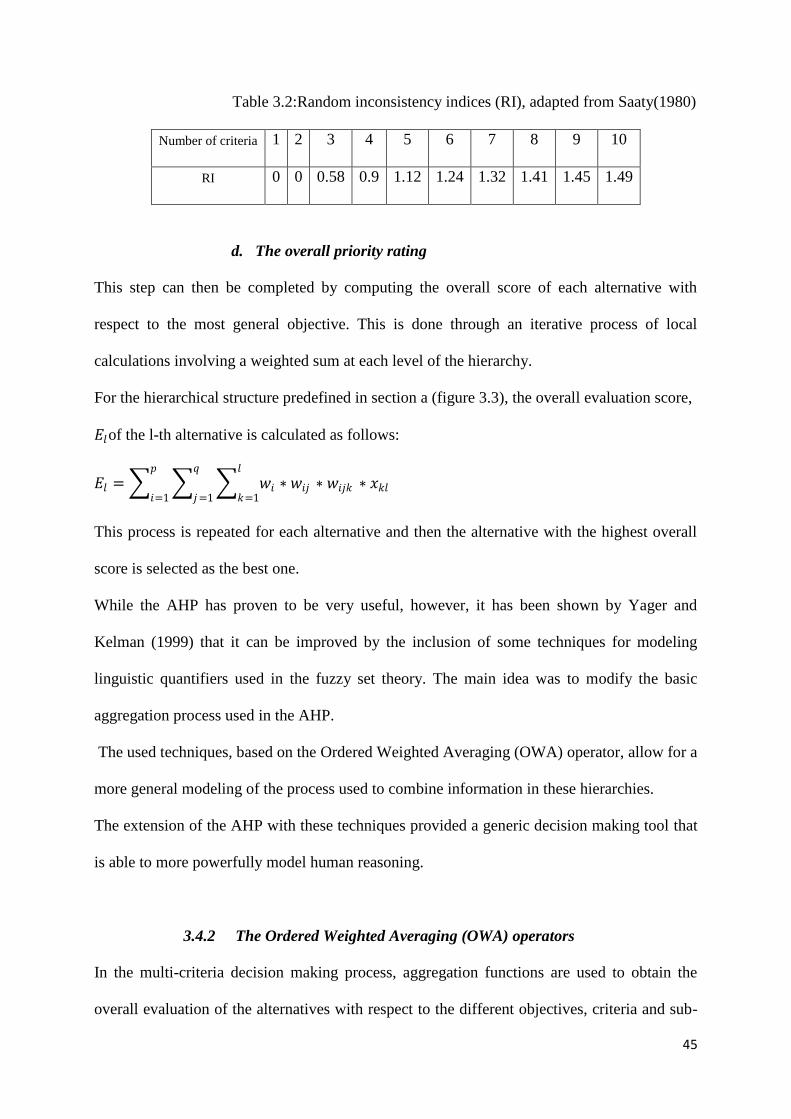
45

Table 3.2:Random inconsistency indices (RI), adapted from Saaty(1980)

Number of criteria 1 2 3 4 5 6 7 8 9 10

RI 0 0 0.58 0.9 1.12 1.24 1.32 1.41 1.45 1.49

d. The overall priority rating

This step can then be completed by computing the overall score of each alternative with

respect to the most general objective. This is done through an iterative process of local

calculations involving a weighted sum at each level of the hierarchy.

For the hierarchical structure predefined in section a (figure 3.3), the overall evaluation score,

𝐸𝑙of the l-th alternative is calculated as follows:

𝐸𝑙 = 𝑤𝑖 ∗ 𝑤𝑖𝑗 ∗ 𝑤𝑖𝑗𝑘 ∗ 𝑥𝑘𝑙

𝑙

𝑘=1

𝑞

𝑗=1

𝑝

𝑖=1

This process is repeated for each alternative and then the alternative with the highest overall

score is selected as the best one.

While the AHP has proven to be very useful, however, it has been shown by Yager and

Kelman (1999) that it can be improved by the inclusion of some techniques for modeling

linguistic quantifiers used in the fuzzy set theory. The main idea was to modify the basic

aggregation process used in the AHP.

The used techniques, based on the Ordered Weighted Averaging (OWA) operator, allow for a

more general modeling of the process used to combine information in these hierarchies.

The extension of the AHP with these techniques provided a generic decision making tool that

is able to more powerfully model human reasoning.

3.4.2 The Ordered Weighted Averaging (OWA) operators

In the multi-criteria decision making process, aggregation functions are used to obtain the

overall evaluation of the alternatives with respect to the different objectives, criteria and sub-

46

criteria considered. Generally, the construction of these aggregation functions must reflect a

number of considerations. Referring to Yager and Kelma, (1999), the two most important

ones are:

- The first consideration is the relationship between the criteria and the sub-criteria

respectively; as perceived by the decision maker. At this level, there are some relevant

questions to ask: ―Does he desire all criteria and sub-criteria respectively to be satisfied?‖,

―Will he be happy if most of them are satisfied?‖, ―Is there some proportion of criteria and

sub-criteria respectively; whose satisfaction is required for an acceptable solution?‖

To answer these different questions, Yager (1988) suggested an approach allowing for a

parameterization of the agenda the decision maker can use to aggregate the relevant criteria,

and sub-criteria respectively. This parameterization allows to go from the extreme of

requiring ―all criteria‖ to be satisfied, to the other extreme of requiring ―at least one criterion‖

to be satisfied, and includes the case of taking the average of the criteria scores.

- The second consideration is the relative importance or the weights of the criteria. This

allows the decision maker to emphasize such or such criterion relatively to the other ones, so

that its impact on the overall aggregative process will be higher.

These two concepts, though are totally different, are included in a same aggregation operator,

the OWA operator.

a. The OWA operators: definition and properties

OWA operators are a generalization of the original decision-making process suggested by

Bellman and Zadeh (1970), and were introduced by Yager (1988) as a tool for decision-

making in a fuzzy environment, where the criteria were fuzzy subsets over the space of

decision alternatives, and each alternative satisfies a single criterion with a degree of

47

satisfaction lying in the unit interval [0, 1]. This degree of satisfaction can also be interpreted

as a membership degree, putting the problem in a fuzzy environment.

Based on Yager (1993), an aggregation operator F:

𝐹: 𝐼𝑛 → 𝐼 , 𝑤𝑕𝑒𝑟𝑒 𝐼 ∈ 0,1

is called an ordered weighted averaging (OWA) operator of dimension n if it has associated

with it a weighting vector W :

𝑊 = 𝑊1

⋮𝑊𝑛

Such that:

(1) 𝑊𝑖 ∈ 0,1

(2) 𝑊𝑖 = 1𝑛𝑖=1

and

(3) 𝐹 𝑐1, 𝑐2, … , 𝑐𝑛 = 𝑑𝑗𝑊𝑗𝑛𝑗=1

Where 𝑏𝑗 is the j-th largest element of the {𝑐1, 𝑐2, … , 𝑐𝑛}. The weights 𝑊𝑗 are not associated

with a particular argument 𝑎𝑖 but with the ordered position of the arguments 𝑑𝑗 .

Example:

Assume:

𝑊 =

0.40.30.20.1

, then

𝑓 0.7, 1, 0.3, 0.6 =(1)(0.4)+(0.7)(0.3)+(0.6)(0.2)+(0.3)(0.1)=0.76 .

Yager (1988) showed that the OWA have the following properties:

Commutativity: the indexing of the arguments is irrelevant.

Monotonicity: if ∀ 𝑖 𝑐𝑖 ≥ 𝑐′𝑖 then 𝐹 𝑐1, 𝑐2, … , 𝑐𝑛 ≥ 𝐹 𝑐′1, 𝑐′2, … , 𝑐′𝑛 .

Idempotency: 𝐹 𝑐, 𝑐, … , 𝑐 = 𝑐

48

These properties imply that the OWA operator is a mean operator (Dubois and Prade, 1985),

and it can be shown that ∀ 𝑐1, 𝑐2, … , 𝑎𝑛 𝑀𝑎𝑥𝑖 𝑐𝑖 ≥ 𝐹 𝑐1, 𝑐2, … , 𝑐𝑛 ≥ 𝑀𝑖𝑛𝑖[𝑐𝑖].

Min, Max, and the Mean are also special cases of the OWA aggregation as they can be

obtained with specific weighting vectors:

- If 𝑊1 = 1 and 𝑊𝑗 = 0 for 𝑗 ≠ 1, then 𝐹 𝑐1, 𝑐2, … , 𝑐𝑛 = 𝑀𝑎𝑥𝑖 𝑐𝑖

- If 𝑊𝑛 = 1 and 𝑊𝑖 = 0 for 𝑖 ≠ 𝑛, then 𝐹 𝑐1, 𝑐2, … , 𝑐𝑛 = 𝑀𝑖𝑛𝑖 𝑐𝑖

- If 𝑊𝑖 = 1𝑛 ∀ 𝑖 then 𝐹 𝑐1, 𝑐2, … , 𝑐𝑛 =

1

𝑛 𝑐𝑖

𝑛𝑖=1

b. Fuzzy logic quantifier-guided OWA combination

Fuzzy linguistic quantifiers were introduced by Zadeh (1983). In accordance to Yager and

Kelman(1999), there are two general classes of linguistic quantifiers: absolute and relative

quantifiers. Absolute quantifiers can be used to represent linguistic terms such ‗as about 5‘ or

‗more than 3‘.However, the relative quantifiers are closely related to imprecise proportions.

They can be represented as fuzzy subsets over the unit interval, with proportional fuzzy

statements such as ‗few‘, ‗half‘, ‗many‘, etc.

In the framework of this thesis, we will only consider the class of the relative quantifiers

known as the regular increasing monotone (RIM) quantifiers.

According to Zadeh (1983), if a fuzzy subset corresponding to a relative linguistic quantifier

is denoted Q, then for any value r in the unit interval, the membership grade Q(r) corresponds

to the compatibility of the value r with the concept which Q is representing.

A general form of a linguistically quantified statement is:

Q of Y are P

where Q is the linguistic quantifier (e.g., all, at least one, most), Y is a class of

objects (e.g., the important criteria, the objectives) and P is some property (e.g., satisfied).

49

When we have 𝐶1, … , 𝐶𝑛 criteria represented as fuzzy subsets over the set of alternatives A,

then the relationship between the criteria can be perceived by the decision maker as:

‘Q criteria are satisfied by an acceptable solution’

A natural question in the definition of the fuzzy linguistic OWA operator is how to

obtain the associated weighting vector. Yager (1988) suggested an interesting way to

compute the weights of OWA operator using fuzzy logic quantifiers, which are given by the

following expression:

𝑊𝑖 = 𝑄 𝑖

𝑛 − 𝑄

𝑖−1

𝑛 , 𝑖 = 1, … , 𝑛

The non-decreasing relative quantifier, Q, is defined by Zadeh(1983) as:

𝑄 𝑟 =

0 𝑖𝑓 𝑟 < 𝛼𝑟 − 𝛼

𝛽 − 𝛼 𝑖𝑓 𝛼 ≤ 𝑟 ≤ 𝛽

1 𝑖𝑓 𝑟 > 𝛽

with 𝛼 , 𝛽 , 𝑟 ∈ [0, 1] and Q(r) indicating the degree to which the proportion r is compatible

with the meaning of the quantifier it represents.

Possible graphic representations of some non-decreasing relative quantifiers are shown in

figure 3.4, where the parameters (𝛼 ; 𝛽) are (0.3; 0.8), (0; 0.5) and (0.5; 1), respectively.

Quantifier: At least half Quantifier: Most Quantifier: As many as possible

Figure 3.4:Monotonically non-decreasing fuzzy linguistic quantifier (Herrera et al., 2000)

50

For each alternative A, the overall satisfaction S(A) is:

𝑒 𝐴 = 𝐹 𝐶1 𝐴 , 𝐶2 𝐴 , 𝐶3 𝐴 , … , 𝐶𝑛 𝐴

where F is an OWA aggregation using the weighting previously determined, and 𝐶𝑖 𝐴 is the

satisfaction of alternative 𝐴 to criteria 𝐶𝑖 .

Some special cases are interesting to note:

- If Q = ‗All‘ , 𝑄 1 = 1, 𝑎𝑛𝑑 𝑄 𝑟 = 0 𝑖𝑓 𝑟 ≠ 1, thus 𝑊𝑛 = 1 𝑎𝑛𝑑 𝑊𝑖 = 0 𝑖𝑓 𝑖 ≠ 𝑛

which means that

𝑒 𝐴 = 𝑀𝑖𝑛𝑖 𝐶𝑖(𝐴)

- If Q = ‗At least one‘, 𝑄 0 = 0, 𝑎𝑛𝑑 𝑄 𝑟 = 1 𝑖𝑓 𝑟 ≠ 0,thus 𝑊1 = 1 𝑎𝑛𝑑 𝑊𝑖 =

0 𝑖𝑓 𝑖 ≠ 1 which means that

𝑒 𝐴 = 𝑀𝑎𝑥𝑖 𝐶𝑖(𝐴)

- If Q is such that 𝑄 𝑟 = 𝑟 , thus 𝑊𝑖 =1

𝑛 which means that

𝑒 𝐴 =1

𝑛 𝐶𝑖(𝐴)

𝑖

which is the average of the satisfactions.

Hence we see that using the operator in combination with the concept of the linguistic

quantifiers provides a useful methodology for formulating multi-criteria formulation

functions.

c. Inclusion of the importances in OWA operators

Yager(1996) suggested a method to evaluate the decision function for the situation where

each of the criteria has an associated importance, and the overall aggregation function is of

the form:

‘Q of the important criteria are satisfied by an acceptable solution’

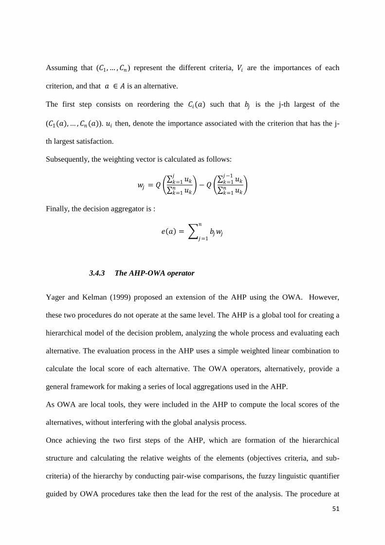
51

Assuming that (𝐶1, … , 𝐶𝑛 ) represent the different criteria, 𝑉𝑖 are the importances of each

criterion, and that 𝑎 ∈ 𝐴 is an alternative.

The first step consists on reordering the 𝐶𝑖(𝑎) such that 𝑏𝑗 is the j-th largest of the

(𝐶1(𝑎), … , 𝐶𝑛(𝑎)). 𝑢𝑖 then, denote the importance associated with the criterion that has the j-

th largest satisfaction.

Subsequently, the weighting vector is calculated as follows:

𝑤𝑗 = 𝑄 𝑢𝑘

𝑗𝑘=1

𝑢𝑘𝑛𝑘=1

− 𝑄 𝑢𝑘

𝑗−1𝑘=1

𝑢𝑘𝑛𝑘=1

Finally, the decision aggregator is :

𝑒 𝑎 = 𝑏𝑗𝑤𝑗

𝑛

𝑗=1

3.4.3 The AHP-OWA operator

Yager and Kelman (1999) proposed an extension of the AHP using the OWA. However,

these two procedures do not operate at the same level. The AHP is a global tool for creating a

hierarchical model of the decision problem, analyzing the whole process and evaluating each

alternative. The evaluation process in the AHP uses a simple weighted linear combination to

calculate the local score of each alternative. The OWA operators, alternatively, provide a

general framework for making a series of local aggregations used in the AHP.

As OWA are local tools, they were included in the AHP to compute the local scores of the

alternatives, without interfering with the global analysis process.

Once achieving the two first steps of the AHP, which are formation of the hierarchical

structure and calculating the relative weights of the elements (objectives criteria, and sub-

criteria) of the hierarchy by conducting pair-wise comparisons, the fuzzy linguistic quantifier

guided by OWA procedures take then the lead for the rest of the analysis. The procedure at

52

this stage involves three main steps (Malczewski, 2006b): (i) specifying the linguistic

quantifier Q, (ii) generating a set of ordered weights associated with Q, and (iii) computing

the overall evaluation for each alternative at each level of the hierarchy by means of the OWA

combination function.

As the criterion weights given by the AHP have the property 𝑊𝑤𝑖 = 1𝑛𝑖=1 , therefore

𝑢𝑘 = 1𝑛𝑘=1 , and the weighting vector and the decision aggregator are then of the form:

𝑤𝑗 = 𝑄 𝑢𝑘

𝑗

𝑘=1 − 𝑄 𝑢𝑘

𝑗−1

𝑘=1

𝑒 𝑎 = 𝑏𝑗𝑤𝑗

𝑛

𝑗=1

3.5 Phase II: The supply chain network design

At each product life cycle stage; and taking into account the efficiency scores that already

have been calculated in the previous phase, the capacity and the demand satisfaction

constraints; the supply chain network design framework needs to identify the effective supply

chain actors as well as the deployment plans.

The proposed model allows identifying, at each product life cycle stage, the optimal routing

of material from the selected suppliers to manufacturers to warehouses by minimizing the

supply chain total cost.

Notations

To formulate the problem, the following parameters are used:

𝐶𝐹𝑖 ,𝑡 Fixed cost to operate the supplier i at stage t

𝐶𝐹𝑗 ,𝑡 Fixed cost to operate the producer j at stage t

𝐶𝐹𝑘 ,𝑡 Fixed cost to operate the distributor k at stage t

53

𝐶𝑂𝑖,𝑡 Fixed cost of opening the supplier i at stage t

𝐶𝑂𝑗 ,𝑡 Fixed cost of opening the producer j at stage t

𝐶𝑂𝑘 ,𝑡 Fixed cost of opening the distributor k at stage t

𝐶𝐶𝑖 ,𝑡 Fixed cost of closing the supplier i at stage t

𝐶𝐶𝑗 ,𝑡 Fixed cost of closing the producer j at stage t

𝐶𝐶𝑘 ,𝑡 Fixed cost of closing the distributor k at stage t

ci,j,t Unit production and transportation cost from supplier i to producer j , at stage t

cj,k,t Unit production and transportation cost from producer j to distributor k, at stage t

ck,z,t Unit production and transportation cost from distributor k to customer zone z, at stage t

ei,t Mean efficiency score of the supplier i, at stage t

ej,t Mean efficiency score of the producer j, at stage t

ek,t Mean efficiency score of the distributor k, at stage t

𝐸𝑒𝑥𝑝𝐼,𝑡 The minimum expected group efficiency average set forth by the decision maker for the

suppliers at stage t

𝐸𝑒𝑥𝑝𝐽 ,𝑡

The minimum expected group efficiency average set forth by the decision maker for the

producers at stage t

𝐸𝑒𝑥𝑝𝐾,𝑡

The minimum expected group efficiency average set forth by the decision maker for the

distributors at stage t

𝑐𝑎𝑝𝑖 ,𝑡 Capacity limit of the supplier i , at stage t

𝑐𝑎𝑝𝑗 ,𝑡 Capacity limit of the producer j, at stage t

𝑐𝑎𝑝𝑘 ,𝑡 Capacity limit of the distributor k at stage t

𝐷𝑧 ,𝑡 Minimum downstream demand of the customer zone z, at stage t

Decision variables:

𝑋𝑖,𝑡 =1 if the supplier i is selected at stage t,

0 otherwise

𝑌𝑗 ,𝑡 =1 if the producer j is selected at stage t,

0 otherwise

𝑍𝑘 ,𝑡 =1 if the distributor k is selected at stage t,

54

0 otherwise

𝑄𝑖 ,𝑗 ,𝑡 Quantity shipped from supplier i to producer j, at stage t, in Ton

𝑄𝑗 ,𝑘 ,𝑡 Quantity shipped from producer j to distributor k, at stage t, in Ton

𝑄𝑘 ,𝑧 ,𝑡 Quantity shipped from distributor k to customer zone z, at stage t, in Ton

𝑖 = 1, … , 𝑚,

𝑗 = 1, … , 𝑛,

𝑘 = 1, … , 𝑝,

𝑧 = 1, … , 𝑞

3.5.1 The mathematical model

The effective multi-period supply chain network design problem, can be formulated as

follows:

min 𝑓 = 𝐶𝐹𝑖 ,𝑡 ∗ 𝑋𝑖 ,𝑡 + 𝐶𝐹𝑗 ,𝑡 ∗ 𝑌𝑗 ,𝑡 + 𝐶𝐹𝑘 ,𝑡

𝑝

𝑘=1

𝑛

𝑗=1

𝑚

𝑖=1∗ 𝑍𝑘 ,𝑡

𝑡

+ 𝐶𝑂𝑖,𝑡 ∗ 𝑋𝑖,𝑡 ∗ 1 − 𝑋𝑖 ,𝑡−1 𝑖∈𝐼

+ 𝐶𝑂𝑗 ,𝑡 ∗ 𝑌𝑗 ,𝑡 ∗ 1 − 𝑌𝑗 ,𝑡−1 + 𝐶𝑂𝑘 ,𝑡𝑘∈𝐾𝑗∈𝐽

∗ 𝑍𝑘 ,𝑡 ∗ 1 − 𝑍𝑘 ,𝑡−1

+ 𝐶𝐶𝑖 ,𝑡 ∗ 𝑋𝑖 ,𝑡 ∗ 1 − 𝑋𝑖,𝑡+1 𝑖∈𝐼

+ 𝐶𝐶𝑗 ,𝑡 ∗ 𝑌𝑗 ,𝑡 ∗ 1 − 𝑌𝑗 ,𝑡+1 + 𝐶𝐶𝑘 ,𝑡𝑘∈𝐾𝑗∈𝐽

∗ 𝑍𝑘 ,𝑡 ∗ (1 − 𝑍𝑘 ,𝑡+1)

+ 𝑐𝑖 ,𝑗 ,𝑡 ∗ 𝑄𝑖,𝑗 ,𝑡 + 𝑐𝑗 ,𝑘 ,𝑡 ∗ 𝑄𝑗 ,𝑘 ,𝑡

𝑝

𝑘=1

𝑛

𝑗=1

𝑛

𝑗=1

𝑚

𝑖=1

+ 𝑐𝑘 ,𝑧,𝑡 ∗ 𝑄𝑘 ,𝑧 ,𝑡 𝑞

𝑧=1

𝑝

𝑘=1 (1)

s.t

Efficiency constraints:

𝑒𝑖 ,𝑡𝑋𝑖,𝑡 ≥ 𝐸𝑒𝑥𝑝𝐼,𝑡 𝑋𝑖,𝑡 ∀ 𝑖, 𝑡 (2)

55

𝑒𝑗 ,𝑡𝑌𝑗 ,𝑡 ≥ 𝐸𝑒𝑥𝑝𝐽 ,𝑡 𝑌𝑗 ,𝑡 ∀ 𝑗, 𝑡 (3)

𝑒𝑘 ,𝑡𝑍𝑘 ,𝑡 ≥ 𝐸𝑒𝑥𝑝𝐾,𝑡 𝑍𝑘 ,𝑡 ∀ 𝑘, 𝑡 (4)

Capacity limits constraints:

𝑄𝑖 ,𝑗 ,𝑡 ≤ 𝑐𝑎𝑝𝑖,𝑡 ∗ 𝑋𝑖,𝑡 ∀ 𝑖𝑛

𝑗=1, 𝑡

(5)

𝑄𝑗 ,𝑘 ,𝑡 ≤ 𝑐𝑎𝑝𝑗 ,𝑡 ∗ 𝑌𝑗 ,𝑡 ∀𝑗𝑝

𝑘=1, 𝑡

(6)

𝑄𝑘 ,𝑧,𝑡 ≤ 𝑐𝑎𝑝𝑘 ,𝑡 ∗ 𝑍𝑘 ,𝑡 ∀𝑘𝑞

𝑧=1, 𝑡

(7)

Flow conservation constraints

𝑄𝑖 ,𝑗 ,𝑡 − 𝑄𝑗 ,𝑘 ,𝑡 = 0 ∀ 𝑗 , 𝑡 𝑝

𝑘=1

𝑚

𝑖=1

(8)

𝑄𝑗 ,𝑘 ,𝑡 − 𝑄𝑘 ,𝑧 ,𝑡

𝑞

𝑧=1= 0 ∀ 𝑘 , 𝑡

𝑛

𝑗=1

(9)

Total market demand satisfaction constraint:

𝑄𝑘 ,𝑧 ,𝑡 ≥ 𝐷𝑧 ,𝑡 ∀ 𝑧, 𝑡 𝑝

𝑘=1

(10)

Non-negativity constraints

𝑄𝑖 ,𝑗 ,𝑡 ≥ 0 ∀ 𝑖, 𝑗 , 𝑡 (11)

𝑄𝑗 ,𝑘 ,𝑡 ≥ 0 ∀ 𝑗, 𝑘, 𝑡 (12)

𝑄𝑘 ,𝑧 ,𝑡 ≥ 0 ∀ 𝑘, 𝑧, 𝑡 (13)

𝑋𝑖,𝑡 ∈ 0,1 ∀𝑖, 𝑡 (14)

𝑌𝑗 ,𝑡 ∈ 0,1 ∀𝑗, 𝑡 (15)

𝑍𝑘 ,𝑡 ∈ 0,1 ∀𝑘, 𝑡 (16)

In the above formulation, the objective function minimizes the supply chain total cost which

includes fixed and variable costs. The variable costs consist of the purchasing costs, the

production costs, and the distribution costs. While the fixed costs consist of the facilities

56

opening costs, operating costs, and closing costs. The opening costs occur at the period t+1

only if the corresponding facility was closed on the previous period t. Simultaneously, for the

closing costs, they occur at a period t only if the corresponding facility was opened at the

period t-1. These two costs are related to the dynamic nature of the problem. At t=0, we

suppose that all facilities are closed.

Constraint sets (2)-(4) prohibit the selection of ineffective actors. Constraint sets (5)-(7)

stipulate that all shipments from a supplier, a plant, or a distribution center must not exceed

their maximum capacity. Constraint sets (8)-(9) indicate a conservation of flow at each

facility, while (10) requires that all the market demand must be met. A non-negativity on each

shipment is imposed by constraint sets (11)-(13). Constraint sets (14)-(16) restrict every

facility to be either open or closed.

3.5.2 The model reformulation

The multi-period nature of the problem is related to the first objective function formulation

(1) which involves the closing and reopening costs. The formulation of these costs includes

nonlinear components and makes the problem quadratic.

However, the binary quadratic problems are known to be NP-hard problems which are also

practically difficult to solve (Liberti, 2007). Basically, the available solution procedures for

the quadratic programming problem may be classified as attempting either to solve the

problem directly or to transform it into an equivalent linear mixed-integer program, and then

solve the latter problem.

In this thesis, we will use the second solution procedure, namely the linearization of the

mathematical model using the method proposed by Fortet (1960). The method consists of

linearizing a 0-1 polynomial programming problem by replacing each polynomial term

𝑋𝑖 ∗ 𝑋𝑗 with a single additional variable and two auxiliary linear constraints.

57

Therefore, the financial function is rewritten as:

min 𝑓 = 𝐶𝐹𝑖 ,𝑡 ∗ 𝑋𝑖,𝑡 + 𝐶𝐹𝑗 ,𝑡 ∗ 𝑌𝑗 ,𝑡 + 𝐶𝐹𝑘 ,𝑡𝑘∈𝐾𝑗∈𝐽𝑖∈𝐼

∗ 𝑍𝑘 ,𝑡 𝑡∈𝑇

+ 𝐶𝑂𝑖,𝑡 ∗ 𝑋𝑖,𝑡 − 𝑋𝑂𝑖,𝑡 + 𝐶𝑂𝑗 ,𝑡 ∗ 𝑌𝑗 ,𝑡 − 𝑌𝑂𝑗 ,𝑡 + 𝐶𝑂𝑘 ,𝑡𝑘∈𝐾𝑗∈𝐽𝑖∈𝐼

∗ 𝑍𝑘 ,𝑡 − 𝑍𝑂𝑘 ,𝑡

+ 𝐶𝐶𝑖 ,𝑡 ∗ 𝑋𝑖,𝑡 − 𝑋𝐶𝑖,𝑡 + 𝐶𝐶𝑗 ,𝑡 ∗ 𝑌𝑗 ,𝑡 − 𝑌𝐶𝑗 ,𝑡 + 𝐶𝐶𝑘 ,𝑡𝑘∈𝐾𝑗∈𝐽𝑖∈𝐼

∗ (𝑍𝑘 ,𝑡 − 𝑍𝐶𝑘 ,𝑡)

+ 𝑐𝑖 ,𝑗 ,𝑡 ∗ 𝑄𝑖,𝑗 ,𝑡 + 𝑐𝑗 ,𝑘 ,𝑡 ∗ 𝑄𝑗 ,𝑘 ,𝑡𝑘∈𝐾𝑗∈𝐽𝑗∈𝐽𝑖∈𝐼

+ 𝑐𝑘 ,𝑧 ,𝑡 ∗ 𝑄𝑘 ,𝑧,𝑡𝑧∈𝑍𝑘∈𝐾

(17)

With

𝑋𝑂𝑖,𝑡 = 𝑋𝑖,𝑡 ∗ 𝑋𝑖,𝑡−1 ∀ i, t (18)

𝑌𝑂𝑗 ,𝑡 = 𝑌𝑗 ,𝑡 ∗ 𝑌𝑗 ,𝑡−1 ∀ j, t (19)

𝑍𝑂𝑘 ,𝑡 = 𝑍𝑘 ,𝑡 ∗ 𝑍𝑘 ,𝑡−1 ∀ k,t (20)

𝑋𝐶𝑖 ,𝑡 = 𝑋𝑖,𝑡 ∗ 𝑋𝑖 ,𝑡+1 ∀ i, t (21)

𝑌𝐶𝑗 ,𝑡 = 𝑌𝑗 ,𝑡 ∗ 𝑌𝑗 ,𝑡+1 ∀ j, t (22)

𝑍𝐶𝑘 ,𝑡 = 𝑍𝑘 ,𝑡 ∗ 𝑍𝑘 ,𝑡+1 ∀ k, t (23)

For linearization, the following constraints are added to the previous problem constraints:

58

Linearization constraints

The set of equations (18)-(23) represent the replacement of the product of the binary variables

by a new additional variable. The constraint sets (24)-(41) was added to force the equality

between the product of the binary variables and the new additional variable.

𝑋𝑂𝑖,𝑡 ≤ 𝑋𝑖 ,𝑡 ∀ 𝑖 (24)

𝑌𝑂𝑗 ,𝑡 ≤ 𝑌𝑗 ,𝑡 ∀ 𝑗 (25)

𝑍𝑂𝑘 ,𝑡 ≤ 𝑍𝑘 ,𝑡 ∀ 𝑘 (26)

𝑋𝑂𝑖,𝑡 ≤ 𝑋𝑖 ,𝑡−1 ∀ 𝑖 (27)

𝑌𝑂𝑗 ,𝑡 ≤ 𝑌𝑗 ,𝑡−1 ∀ 𝑗 (28)

𝑍𝑂𝑘 ,𝑡 ≤ 𝑍𝑘 ,𝑡−1 ∀ 𝑘 (29)

𝑋𝑂𝑖,𝑡 ≥ 𝑋𝑖 ,𝑡 + 𝑋𝑖,𝑡−1 − 1 ∀ 𝑖 (30)

𝑌𝑂𝑖 ,𝑡 ≥ 𝑌𝑖 ,𝑡 + 𝑌𝑖 ,𝑡−1 − 1 ∀ 𝑗 (31)

𝑍𝑂𝑖,𝑡 ≥ 𝑍𝑖 ,𝑡 + 𝑍𝑖 ,𝑡−1 − 1 ∀ 𝑘 (32)

𝑋𝐶𝑖 ,𝑡 ≤ 𝑋𝑖,𝑡 ∀ 𝑖 (33)

𝑌𝐶𝑗 ,𝑡 ≤ 𝑌𝑗 ,𝑡 ∀ 𝑗 (34)

𝑍𝐶𝑘 ,𝑡 ≤ 𝑍𝑘 ,𝑡 ∀ 𝑘 (35)

𝑋𝐶𝑖 ,𝑡 ≤ 𝑋𝑖,𝑡−1 ∀ 𝑖 (36)

𝑌𝐶𝑗 ,𝑡 ≤ 𝑌𝑗 ,𝑡−1 ∀ 𝑗 (37)

𝑍𝐶𝑘 ,𝑡 ≤ 𝑍𝑘 ,𝑡−1 ∀ 𝑘 (38)

𝑋𝐶𝑖 ,𝑡 ≥ 𝑋𝑖,𝑡 + 𝑋𝑖,𝑡−1 − 1 ∀ 𝑖 (39)

𝑌𝐶𝑗 ,𝑡 ≥ 𝑌𝑗 ,𝑡 + 𝑌𝑗 ,𝑡−1 − 1 ∀ 𝑗 (40)

𝑍𝐶𝑘 ,𝑡 ≥ 𝑍𝑘 ,𝑡 + 𝑍𝑘 ,𝑡−1 − 1 ∀ 𝑘 (41)

59

3.6 Case study

This section presents a case study supply chain design problem adapted from a real-life

situation. The purpose is neither to show any advantage of the modeling process by

comparing it with other MIP models, nor to exhibit the efficiency of problem solving by

benchmarking the computation time to other algorithms. Indeed, we aim at illustrating the

effectiveness and convenience of the product life cycle consideration in the supply chain

design, by introducing a multi-criteria decision making and multi-objective models to select

the effective supply chain actors in the different product life cycles' stages. We consider the

case of a focal company which is in the launching process of a new product on the market,

namely, the environmentally coal from the olive pomace. The company has to design its

supply chain with a minimal cost, considering the product life cycle stages.

To reach this goal, we apply the two- phase proposed model.

Phase 1: A multi-criteria decision making problem to evaluate the potential actors‘ efficiency

Table 3.3, revised from Wang et al. (2009), lists an integral description of the different criteria

and sub-criteria considered,and the corresponding original scale measurement. This table will

be adapted to our case study for the three different business process types, namely

procurement, production and distribution processes. Numerical and linguistic interval scales

are used in this method. Figure 3.5 presents the linguistic rating on membership function

corresponding to fuzzy numbers (Herrera et al. 2000).

60

Table 3.3: The core of factors on supply chain performance

Criteria Attributes

Original

scale

R&D

Design L

Technique L

Innovation L

Cost

Normal unit cost N

Minimum order quantity N

Discount N

Quality

Characteristic 1 N

Characteristic 2 N

Characteristic 3 N

Service

Flexibility N

Stockout N

Additioal service L

Response

Normal delivery lead-time N

Requiring lead-time to changing volume N

Requiring lead-time to changing design N

Minimum delivery lead-time N

―L‖ means linguistic scale; ―N‖ means numerical scale

Figure 3.5:Linguistic rating on membership function corresponding to fuzzy number

61

The table 3.4 presents the data collection of the predefined criteria and sub-criteria, relative to

the set of the potential suppliers.

Table 3.4:Data collection on supply performance

Criteria Attributes S1 S 2 S 3 S 4 S 5 S 6

R&D

Grinding technique 0.67 0.5 0.5 0.33 0.5 0.5

Drying technique 0.67 0.67 0.5 0.67 0.67 0.33

Innovation 0.5 0.5 0.67 0.5 0.67 0.5

Cost

Fixed cost in € 5000 3000 0 5000 0 3000

Normal unit cost in € 55 50 52 53 53 55

Minimum order quantity in Ton 2000 2000 1000 2000 2000 1000

Quality

Humidity 0.08 0.1 0.06 0.05 0.08 0.1

Rate of oil 0.03 0.025 0.02 0.02 0.03 0.025

Grain size in mm 2 2 1.5 3 2.5 3

Service

Packaging 90% 95% 85% 95% 99% 90%

Stockout 2% 8% 5% 6% 8% 2%

Additional service 99% 99% 95% 90% 95% 99%

Response

Normal delivery lead-time in

week

4 3 3 2 4 4

Requiring lead-time to changing

volume in week

2 2 1 1 2 1

Requiring lead-time to changing

design in week

1 1 1 1 2 1

The AHP components weights:

The component weights and the different scores are given by pairwise comparisons, for each

process at each product life cycle stage, following the AHP method described in section 3.4.1.

62

Considering the set of the potential suppliers, tables 3.5 and 3.6 give the criteria pairwise

comparison and their relative AHP weights, at the introduction and the maturity stages

respectively.

Table 3.5:Criteria pairwise comparison and relative weights at the introduction stage

R&D Cost Quality Service Response Weights

R&D 1 1/9 1/7 1/5 1/5 0.029

Cost 9 1 5 5 7 0.558

Quality 7 1/5 1 3 3 0.209

Service 5 1/5 1/5 1 3 0.126

Response 5 1/7 1/3 1/3 1 0.076

Table 3.6:Criteria pairwise comparison and relative weights at the maturity stage

R&D Cost Quality Service Response Weights

R&D 1 5 3 9 7 0.5128

Cost 1/5 1 1/3 5 3 0.129

Quality 1/3 3 1 7 5 0.2615

Service 1/9 1/5 1/7 1 1/3 0.0333

Response 1/7 1/3 1/5 3 1 0.0634

Table 3.7 gives the pairwise comparison for the sub-criteria relative to the criterion ―R&D‖

and their corresponding weights for the same process ―suppliers‖ at the introduction stage of

the product life cycle.

63

Table 3.7:pairwise comparison of the sub-criteria relative to the criterion ‗R&D‘ and relative

weights

Grinding technique Drying technique Innovation Weights

Grinding technique 1 1/5 5 0.218

Drying technique 5 1 7 0.715

Innovation 1/5 1/7 1 0.067

Following the same logic, the different suppliers‘ AHP-scores relative to the R&D criterion at

the introduction stage are given by the table 3.8.

Table 3.8:AHP scores for the R&D criterion at the introduction stage

S1 S 2 S 3 S 4 S 5 S 6

Grinding technique 0.505 0.116 0.116 0.029 0.116 0.116

Drying technique 0.23 0.23 0.057 0.23 0.23 0.222

Innovation 0.071 0.071 0.357 0.071 0.357 0.071

This same procedure has to be repeated for all the rest of the criteria and their corresponding

sub-criteria at each product life cycle stage.

The remaining details for this case study will be given in the appendix.

In the sequel, to fit the supply chain strategy depending on the importance of the different

criteria, three linguistic quantifiers are used, namely ―At least half‖, ―Most‖, and ―As many as

possible‖.

However, the different criteria and sub-criteria‘ importances are closely related to the

different phases of the product life cycle. Inspired from Aitken et al. (2003), table 3.9

suggested different supply chain strategies adopted in the framework of this thesis to meet the

market demand, in gaining the competitive advantages during the different phases of the

64

product life cycle. These linguistic quantifiers expressing the criteria and sub-criteria

importances, being subjective, could vary from one decision maker to another.

Table 3.9:Product criteria and supply chain strategy on product life cycle

Linguistic Phase

Quantifier

Introduction Growth Maturity Decline

At least half R&D Service Cost Service

Most

Quality

Cost

Response

Cost

Quality

Response

Quality

Service

Response

Cost

Quality

Response

As many as possible Service R&D R&D R&D

The AHP-OWA components weights and final scores:

Returning to our case study the aggregation function is of the form:

At least half of the important criteria are satisfied by an acceptable solution

is considered for the criterion R&D at the introduction stage.

Table 3.10 presents the ordered AHP scores and their corresponding weights, the AHP-OWA

weights, and the final scores.

According to this table, it is noted that for the most important criterion in the introduction

stage, namely, the R&D, the supplier S3 has the highest score, after comes the supplier S1,

and so on.

65

Table 3.10:potential suppliers‘ final scores for the R&D criterion at the introduction stage

Suppliers Ordered AHP Scores AHP weights AHP-OWA weights Final scores

S1

0.505 0.218 0.436

0.349 0.23 0.715 0.564

0.071 0.067 0

S2

0.23 0.715 1

0.23 0.116 0.218 0

0.071 0.067 0

S3

0.357 0.067 0.132

0.511 0.218 0.218 0.436

0.057 0.715 0.432

S4

0.23 0.715 1

0.23 0.071 0.067 0

0.029 0.218 0

S5

0.357 0.067 0.132

0.246 0.23 0.715 0.868

0.116 0.218 0

S6

0.22 0.715 1

0.22 0.116 0.218 0

0.071 0.067 0

This procedure is then repeated for all the rest of the criteria at each product life cycle stage,

and the overall aggregation function considered was of the form:

Most of the important criteria are satisfied by an acceptable solution

Table 3.11 presents the overall efficiency scores obtained by the potential suppliers at the

introduction and the maturity stages.

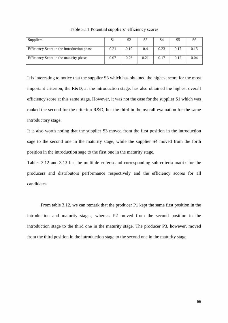
66

Table 3.11:Potential suppliers‘ efficiency scores

Suppliers S1 S2 S3 S4 S5 S6

Efficiency Score in the introduction phase 0.21 0.19 0.4 0.23 0.17 0.15

Efficiency Score in the maturity phase 0.07 0.26 0.21 0.17 0.12 0.04

It is interesting to notice that the supplier S3 which has obtained the highest score for the most

important criterion, the R&D, at the introduction stage, has also obtained the highest overall

efficiency score at this same stage. However, it was not the case for the supplier S1 which was

ranked the second for the criterion R&D, but the third in the overall evaluation for the same

introductory stage.

It is also worth noting that the supplier S3 moved from the first position in the introduction

sage to the second one in the maturity stage, while the supplier S4 moved from the forth

position in the introduction sage to the first one in the maturity stage.

Tables 3.12 and 3.13 list the multiple criteria and corresponding sub-criteria matrix for the

producers and distributors performance respectively and the efficiency scores for all

candidates.

From table 3.12, we can remark that the producer P1 kept the same first position in the

introduction and maturity stages, whereas P2 moved from the second position in the

introduction stage to the third one in the maturity stage. The producer P3, however, moved

from the third position in the introduction stage to the second one in the maturity stage.

67

Table 3.12:Multiple attribute matrix on production performance and efficiency scores Criteria Attributes P1 P 2 P 3

R&D

Grinding technique

0.84 0.5 0.5

Drying

technique

0.84 0.67 0.5

Innovation 0.84 0.5 0.3

Cost

Normal unit cost in €

170 160 155

Minimum order quantity in

Ton

2000 1000 1000

Discount 7% 5% 3%

Quality

Humidity

0.05 0.08 0.08

Rate of oil

0.015 0.025 0.025

Calorific in Mj per Kg 19.8 18.5 18

Service

Packing

0.84 0.67 0.5

Stockout

2% 6% 8%

Additional

service 99% 90% 80%

Response


week 8 10 12

Requiring lead-time to

changing volume in week

2 5 5


changing design in week

3 5 8

Efficiency Score in the introduction phase 0.75 0.18 0.06

Efficiency Score in the maturity phase 0.68 0.19 0.2

68

Table 3.13:Multiple attribute matrix on distribution performance and efficiency scores

Criteria Attributes D1 D 2 D 3

R&D

Technical market timing

0.84 0.67 0.5

Distribution technique

0.84 0.84 0.67

Marketing technique 0.67 0.67 0.5

Cost

Normal unit cost in €

19 19 18

Minimum order quantity in

Ton

500 500 1000

Unit express delivery cost 22 21 20

Quality

Reliability

99% 90% 85%

Stability

99% 98% 95%

Quality business

relashionships 0.84 0.67 0.5

Service

Flexibility

0.84 0.67 0.5

In store advertising

0.67 0.5 0.16

Continuity index in min 170 330 350

Response


week 10 12 8

Minimum delivery lead-time

in week

7 7 5


changing volume in week

3 3 2

Efficiency Score in the introduction phase 0.47 0.32 0.09

Efficiency Score in the maturity phase 0.15 0.19 0.35

69

It is notable from this table that the distributor D1moved from the first position in the

introduction stage to the last one in the maturity stage, the distributor D2 kept the same

second position in these two stages.

Phase 2: The mathematical model for the supply chain design network.

The mathematical model is solved to identify the optimum solution since the introduction of

the product to the market until the sales decline.

Figure 3.6 shows the sales distribution in Ton for the 3 different customer zones.

Figure 3.6:Sales distribution of the product in Ton

Figure 3.7 illustrates the deployment plan of the total supply chain during the product life

cycle.

It is obvious that the transshipment solution for the supply chain network deployment changes

from one stage to another. This is probably due to variables, namely the demand variation, as

well as the efficiency scores variation. Indeed, different supply chain strategies could be

adopted at different phases of the product life cycle, significantly influencing the supply chain

actors‘ selection decisions.

70

Using the same focal company as in the previous section, but keeping the same data on

demand, tables 3.14 and 3.15 illustrate the optimal deployment plans for the supply chain

network or the introduction and the maturity phase respectively.

71

Introduction stage Growth stage Maturity Stage Decline stage

P

1 D

2 Z

1 Z

2 Z

3 P

1 D

1 Z

1 Z

2 Z

3 P

1 P

3 D

2 D

3 Z

1 Z

2 Z

3 P

1 D

1 Z

1 Z

2 Z

3

S1

11200

16500

S2

50000

S3 10000

30000

34500

10000

S4 6000

S5

S6

P1

16000

41200

40500 9500

26500

P2

34500

P3

D1

17500 8500 15200

10000 6500 10000

D2

8000 3500 4500

40500

D3

14000 30000

Demand

>=8000 >=3500 >=4500

>=17500 >=8500 >=15200

>=40500 >=14000 >=30000

>=10000 >=6500 >=10000

Figure 3.7:The deployment plan of the total supply chain

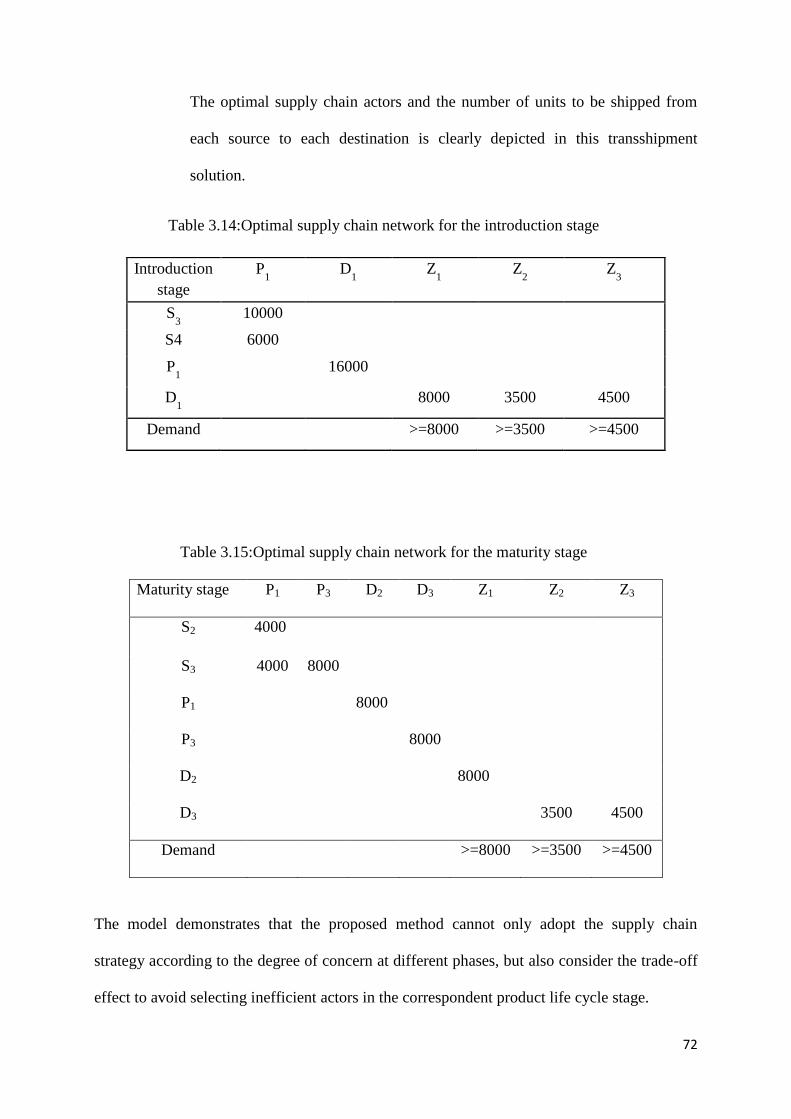
72

The optimal supply chain actors and the number of units to be shipped from

each source to each destination is clearly depicted in this transshipment

solution.

Table 3.14:Optimal supply chain network for the introduction stage

Table 3.15:Optimal supply chain network for the maturity stage

Maturity stage P1 P3 D2 D3 Z1 Z2 Z3

S2 4000

S3 4000 8000

P1 8000

P3 8000

D2 8000

D3 3500 4500

Demand >=8000 >=3500 >=4500

The model demonstrates that the proposed method cannot only adopt the supply chain

strategy according to the degree of concern at different phases, but also consider the trade-off

effect to avoid selecting inefficient actors in the correspondent product life cycle stage.

Introduction

stage

P1 D

1 Z

1 Z

2 Z

3

S3 10000

S4 6000

P1 16000

D1 8000 3500 4500

Demand >=8000 >=3500 >=4500

73

From the listed results in table 3.15 for the maturity phase, it is interesting to notice that

supplier 2, who was considered to be inefficient in the introduction phase, was selected as an

efficient actor in the maturity phase, and similarly for distributor 3. This fact demonstrates

that this method can adopt different supply chain strategies related to the product strategies of

a focal company.

3.7 Model limits:

A case which can occur, and which may be a limitation of the model, is the one relating to the

efficiency and the capacity constraints. Indeed, we can assume the following scenario:

It is possible that among the potential actors examined in phase I, the selected ones as the

most efficient, cannot meet the needs of the supply chain, due to their capacity constraints,

and that the rest of the potential actors are inefficient for selection.

When this scenario occurs, we propose four alternatives in order to solve the problem.

3.7.1 Review the expected efficiency value

In this case, we have to reconsider the expected efficiency value previously set by the

decision maker. This is the easiest alternative to adopt, but nevertheless, we have to ask once

more the decision maker, and he has to agree to reduce the efficiency limit value. However, it

should be noticed that the efficiency bounds must be decreased within a reasonable limit

because of its implications on the overall performance of the supply chain network. We then

can select other actors still, but it is necessary that the new efficiency constraints be satisfied.

3.7.2 Review the sets of the potential actors

Here it is a question of revising the lists of the potential actors, and to add new ones who may

be more effective and can meet the needs of the supply chain in terms of efficiency and

74

capacity. This alternative could be the most relevant, but also the longest and the most

complicated to perform. What makes it not very practical, is the need to redo all the steps of

the first phase to aggregate the new data and recalculate the efficiency scores.

3.7.3 The penalty method

Generally, the penalty function method attempts to approximate a constrained optimization

problem with an unconstrained one and then apply standard search techniques to obtain

solutions. The approximation is accomplished in the case of penalty methods by adding a

term to the objective function that prescribes a high cost for the violation of the constraints.

Consider the problem:

𝑀𝑖𝑛𝑖𝑚𝑖𝑧𝑒 𝑓 𝑥 ∶ 𝑥 ∈ 𝑆 , 𝑥 ∈ 𝑇 𝑃(1)

Where 𝑓 is a continuous function on R𝑛 and 𝑆 is a constraint set in R𝑛 .

The main idea of a penalty function method is to replace problem 𝑃 1 by an unconstrained

approximation of the form:

𝑀𝑖𝑛𝑖𝑚𝑖𝑧𝑒 𝑓 𝑥 + 𝑐𝑃 𝑥 , 𝑥 ∈ 𝑇 𝑃(2)

Where c is a positive constant and 𝑃 is a function on R𝑛 satisfying (i) 𝑃(𝑥) is continuous, (ii)

𝑃 𝑥 ≥ 0 for all 𝑥 ∈ R𝑛 , and (iii) 𝑃 𝑥 = 0 if and only if ∈ 𝑆 .

If the penalty function 𝑃 𝑥 grows quickly enough outside of 𝑆, the optimal solution of 𝑃(1)

will also be optimal for 𝑃(2). Furthermore, any optimal solution of 𝑃(2) will provide an

upper bound on the optimum for 𝑃(1), and this bound will in general be tighter than that

obtained by simply optimizing 𝑓 𝑥 over 𝑇, Smith and Coit (1995).

In our case, the penalty function, replaces the efficiency constraints by adding a term to

the objective function that consists of a penalty parameter and a measure of violation of the

constraints.

http://en.wikipedia.org/wiki/Objective_function

75

We define the following penalty functions:

𝑃𝑖 ,𝑡 𝐼 = ∆𝑖,𝑡𝑋𝑖 ,𝑡 ; 𝑃𝑗 ,𝑡 𝐽 = ∆𝑗 ,𝑡𝑌𝑗 ,𝑡 ; 𝑃𝑘 ,𝑡 𝐾 = ∆𝑘 ,𝑡𝑍𝑘 ,𝑡

with

∆𝑖 ,𝑡= max eexp ,I,t − ei,t , 0 , ∆𝑗 ,𝑡= max eexp ,J,t − ej,t , 0 , ∆𝑘 ,𝑡= max eexp ,K,t − ek,t , 0

Where

ei,t : Mean efficiency score of the supplier i, at stage t

ej,t : Mean efficiency score of the producer j, at stage t

ek,t : Mean efficiency score of the distributor k, at stage t

𝐸𝑒𝑥𝑝𝐼,𝑡 : The minimum expected group efficiency average set forth by the decision maker for

the suppliers at stage t

𝐸𝑒𝑥𝑝𝐽 ,𝑡 : The minimum expected group efficiency average set forth by the decision maker for

the producers at stage t

𝐸𝑒𝑥𝑝𝐾,𝑡 : The minimum expected group efficiency average set forth by the decision maker for

the distributors at stage t

c : The penalty value

The new problem objective function is then as the following:

76

min 𝑓 = 𝑐 ∗ 𝑃𝑖 ,𝑡 𝐼 + 𝑃𝑗 ,𝑡 𝐽 + 𝑃𝑘 ,𝑡 𝐾 𝑘∈𝐾𝑗∈𝐽𝑖∈𝐼

𝑡∈𝑇

+ 𝐶𝐹𝑖 ,𝑡 ∗ 𝑋𝑖 ,𝑡 + 𝐶𝐹𝑗 ,𝑡 ∗ 𝑌𝑗 ,𝑡 + 𝐶𝐹𝑘 ,𝑡𝑘∈𝐾𝑗∈𝐽𝑖∈𝐼

∗ 𝑍𝑘 ,𝑡




∗ (𝑍𝑘 ,𝑡 − 𝑍𝐶𝑘 ,𝑡)



Under the constraints (5)-(16) and (18)-(29).

This method allows the non effective potential actors, but whose efficiency scores are closer

to the expected efficiency value to be selected, allowing us to meet the market demand.

It has however some drawbacks, namely the selection of non-effective actors, which could

affect the overall efficiency of the supply chain.

3.7.4 Capacity extension

Capacity planning is among the most significant capital investment decisions that supply

chain managers must periodically make. In the following, we propose an optimization model

for the strategic capacity planning, which will allow capacity expansion for the effective

supply chain actors that are selected.

In cases where the supply chain actors are still effective; even when the product goes from

one stage to another of its product life cycle; but their respective capacities don‘t allow them

77

to meet the needs of the market, the proposed model will avoid the selection of new actors,

but only a capacity expansion of the preselected ones, to the extent that this operation

complies with the problem objective function and will not increase the supply chain total cost.

Additional model parameters:

𝑐𝑒𝑖 ,𝑡 Unit cost of expanding the capacity of the supplier i at stage t

𝑐𝑒𝑗 ,𝑡 Unit cost of expanding the plant j at stage t

𝑐𝑒𝑘 ,𝑡 Unit cost of expanding the distribution center k at stage t

𝑀𝐸𝑖 ,𝑡 Maximum expansion capacity of the supplier i at stage t

𝑀𝐸𝑗 ,𝑡 Maximum expansion capacity of the plant j at stage t

𝑀𝐸𝑘 ,𝑡 Maximum expansion capacity of the distribution center k at stage t

Additional model decision variables:

𝐸𝑋𝑖 ,𝑡 =1 if the supplier capacity is expanded at stage t,

0 otherwise

𝐸𝑌𝑗 ,𝑡 =1 if the plant is expanded at stage t,

0 otherwise

𝐸𝑍𝑘 ,𝑡 =1 if the distribution center is expanded at stage t,

0 otherwise

𝐶𝑋𝑖,𝑡 Capacity added to the supplier i at stage t

78

𝐶𝑌𝑗 ,𝑡 Capacity added to the plant j at stage t

𝐶𝑍𝑘 ,𝑡 Capacity added to the distribution center k at stage t

min 𝐶𝐹𝑖 ,𝑡 ∗ 𝑋𝑖 ,𝑡𝑖∈∗∗𝐼

+ 𝐶𝐹𝑗 ,𝑡 ∗ 𝑌𝑗 ,𝑡𝑗∈𝐽

+ 𝐶𝐹𝑘 ,𝑡𝑘∈𝐾


+ 𝐶𝑂𝑖 ,𝑡 ∗ 𝑋𝑖 ,𝑡 − 𝑋𝑂𝑖 ,𝑡 𝑖∈𝐼

+ 𝐶𝑂𝑗 ,𝑡 ∗ 𝑌𝑗 ,𝑡 − 𝑌𝑂𝑗 ,𝑡 𝑗∈𝐽

+ 𝐶𝑂𝑘 ,𝑡 ∗ 𝑍𝑘 ,𝑡 − 𝑍𝑂𝑘 ,𝑡 𝑘∈𝐾

+ 𝐶𝐶𝑖 ,𝑡 ∗ 𝑋𝑖 ,𝑡 − 𝑋𝐶𝑖 ,𝑡 𝑖∈𝐼

+ 𝐶𝐶𝑗 ,𝑡 ∗ 𝑌𝑗 ,𝑡 − 𝑌𝐶𝑗 ,𝑡 𝑗∈𝐽

+ 𝐶𝐶𝑘 ,𝑡 ∗ 𝑍𝑘 ,𝑡 − 𝑍𝐶𝑘 ,𝑡 𝑘∈𝐾

+ 𝑐𝑖,𝑗 ,𝑡 ∗ 𝑄𝑖 ,𝑗 ,𝑡𝑗∈𝐽𝑖∈𝐼

+ 𝑐𝑗 ,𝑘 ,𝑡 ∗ 𝑄𝑗 ,𝑘 ,𝑡𝑘∈𝐾𝑗∈𝐽

+ 𝑐𝑘 ,𝑧 ,𝑡 ∗ 𝑄𝑘 ,𝑧 ,𝑡𝑧∈𝑍𝑘∈𝐾

+ 𝑐𝑒𝑖,𝑡 ∗ 𝐸𝑋𝑖 ,𝑡 + 𝑐𝑒𝑗 ,𝑡 ∗ 𝐸𝑌𝑗 ,𝑡 +𝑗∈𝐽

𝑐𝑒𝑘 ,𝑡 ∗ 𝐸𝑍𝑘 ,𝑡𝑘∈𝐾𝑖∈𝐼

Subject to the constraints:

(2)-(4) ,(8)-(16) , (18)-(29), and

79


𝑄𝑖 ,𝑗 ,𝑡 ≤ 𝑐𝑎𝑝𝑖,𝑡 ∗ 𝑋𝑖,𝑡 + 𝐶𝑋𝑖,𝑡 ∀ 𝑖𝑛

𝑗=1, 𝑡 (30)

𝑄𝑗 ,𝑘 ,𝑡 ≤ 𝑐𝑎𝑝𝑗 ,𝑡 ∗ 𝑌𝑗 ,𝑡 + 𝐶𝑌𝑗 ,𝑡 ∀𝑗𝑝

𝑘=1, 𝑡 (31)

𝑄𝑘 ,𝑧,𝑡 ≤ 𝑐𝑎𝑝𝑘 ,𝑡 ∗ 𝑍𝑘 ,𝑡 + 𝐶𝑍𝑘 ,𝑡 ∀𝑘𝑞

𝑧=1, 𝑡

(32)

𝐶𝑋𝑖,𝑡 ≤ 𝑀𝐸𝑖 ,𝑡 ∀ 𝑖 , 𝑡 (33)

𝐶𝑌𝑗 ,𝑡 ≤ 𝑀𝐸𝑗 ,𝑡 ∀ 𝑗 , 𝑡 (34)

𝐶𝑍𝑘 ,𝑡 ≤ 𝑀𝐸𝑘 ,𝑡 ∀ 𝑘 , 𝑡 (35)

An extended site is obligatory opened:

𝐸𝑋𝑖 ,𝑡 ≤ 𝑋𝑖,𝑡 ∀ 𝑖 , 𝑡 (36)

𝐸𝑌𝑗 ,𝑡 ≤ 𝑋𝑗 ,𝑡 ∀ 𝑗 , 𝑡 (37)

𝐸𝑍𝑘 ,𝑡 ≤ 𝑋𝑘 ,𝑡 ∀ 𝑘 , 𝑡 (38)

Non-negativity Constraints :

𝐸𝑋𝑖 ,𝑡 ≥ 0 ∀ 𝑖, 𝑡 (39)

𝐸𝑌𝑗 ,𝑡 ≥ 0 ∀ 𝑗, 𝑡 (40)

𝐸𝑍𝑘 ,𝑡 ≥ 0 ∀ 𝑘, 𝑡 (41)

The constraint sets (30)-(32) stipulate that all shipments from a given supply chain actor must

not exceed its initial capacity plus the capacity added. The constraint sets (33)-(35) state that

the capacity added to each facility must not exceed its maximum capacity extension. The

constraint sets (36)-(38) prohibit extensions to be made for closed facilities. Non-negativity

on each capacity extension is imposed by constraint sets (39)-(41).

80

If we take the same case study as previously, figure 3.8 presents the fluctuations in the

capacity of the supply chain actors of the different processes, over the product life cycle.

Figure 3.8:Fluctuations in capacities over the product life cycle

We can clearly understand ,from this figure, that the capacity extension reaches the highest

level during the growth phase, which is predictable with the increasing of the market demand.

The supply chain total cost however moves from 72 327 800 euro, in the case without a

capacity expansion to 71 022 200 euro in the case when we allow the capacity expansion of

the selected actors, which represents a total gain of 1.8% on the total cost.

3.8 Conclusion

This chapter focuses on the design of a supply chain network for a product from its

introduction to the market to its decline stage. To achieve this goal, we have proposed a two-

phase multi-criteria supply chain design model. In the first phase, we proposed to solve a

multi-criteria decision making problem, taking into account different criteria set by the

decision maker as well as the variation of the importance of these criteria and the

corresponding sub-criteria according to the decision maker‘s preferences, through the product

life cycle stages. The combination of two aggregators was used for this, namely, the AHP and

0

5000

10000

15000

20000

25000

Introduction Growth Matirity Decline

Suppliers

Producers

Distributors

81

the OWA operators, which allowed modeling situations where the number of sub-criteria

needed to satisfy a higher order concept, can be expressed in terms of fuzzy linguistic

quantifiers. In the second phase, we proposed a mathematical model for a multi-period supply

chain design. This methodology should assist managers in effectively designing a supply

chain network by considering a number of criteria such as efficiencies of selecting actors,

capacity limits, and market demand. While the traditional network design models identify the

optimal network by minimizing the total cost, our method integrates additional important

aspects of performance into the decision analysis. From a managerial perspective, this

methodology conceives of a network that can meet the needs of the market by offering low

costs, high on-time delivery rates, high quality levels, and high service quality, according to

the market expectations for each product life cycle stage, which is not easily possible with

traditional cost minimization approaches. The proposed model can also be applied by

companies for reengineering an existing supply chain network in order to improve the overall

performance. In such a situation, a firm can utilize the proposed method for evaluating the

performance of existing suppliers, producers, and distribution centers in the network, and

involve reduction of supply base in decisions by eliminating poorly performing suppliers,

shutting down inefficient producers and reallocating resources to improve the performance for

a given phase of the product life cycle.

Although the proposed methodology has proven an ability to design an effective multi-period

supply chain network, this does not exclude the fact that it may present some limitations

mainly related to the filtering out of the inefficient actors and to the efficiency bounds set by

the decision maker. However, some solutions were proposed to overcome such problems.

In the next chapter, we will extend the mathematical model of our methodology to a multi-

objective supply chain network design model.

82

4.1 Introduction

In the previous chapter, we proposed a two-phase method to design a multi-period supply

chain network which takes into account the different phases the product goes through during

its life cycle. The only objective considered in this method was to minimize the supply chain

total cost.

In this chapter, we propose a method to design a sustainable multi-period supply chain with

product life cycle consideration, while respecting the triple bottom line (3BL) concept. This

concept, also known as ‗three Ps‖ refers succinctly to "people, planet and profit".

In recent years, supply chains have grown tremendously. They have focused only on the

economic performance to optimize the costs or Return On Investments (ROIs), that cannot

alone sustain the development of supply chain operations. The impact of different activities

involved in supply chains such as the process of manufacturing, warehousing, distributing etc.

on environment and social life of city residents cannot be ignored.

Correspondingly, the concepts of Green Supply Chain Management (GSCM) and Sustainable

Supply Chain Management (SSCM) have emerged. They emphasize the importance of

CHAPTER 4

A product-driven sustainable supply chain design

83

implementing environmental and social concerns along with economical factors in supply

chain planning.

Other perspectives from the management field insist on the sustainability, supply chain

management should strive for enterprise governance, business regulations, corporate

responsibilities, and social justice.

The method proposed in this chapter is novel, since it deals with the important problem of

designing supply chain networks to achieve sustainability from socio-economic-

environmental perspective and takes, at the same time, the product life cycle into

consideration.

The chapter is organized as follows: in Section 2, we define the problem, and provide a the

literature review of prior works first, in the supply chain design with product life cycle

considerations, and then in the environmental management field. In Section 3, we present the

two-phase approach taking into consideration sustainability. We first explain the multi-criteria

decision making problem method, and then provide details of the mathematical formulations

for the model proposed. In section 4, we present a numerical example to validate the

consistency of the proposed model. In section 5, we present some sensitivity analysis. We

conclude this chapter by section 6, with some suggestions for future research in this area.

4.2 Problem definition

The overall goal, is to design a sustainable multi-level supply chain, taking into consideration


According to the United Nation Global Compact, the Supply chain sustainability is the

management of economic, environmental, and social impacts, and the encouragement of good

governance practices, throughout the lifecycles of goods and services. The objective of supply

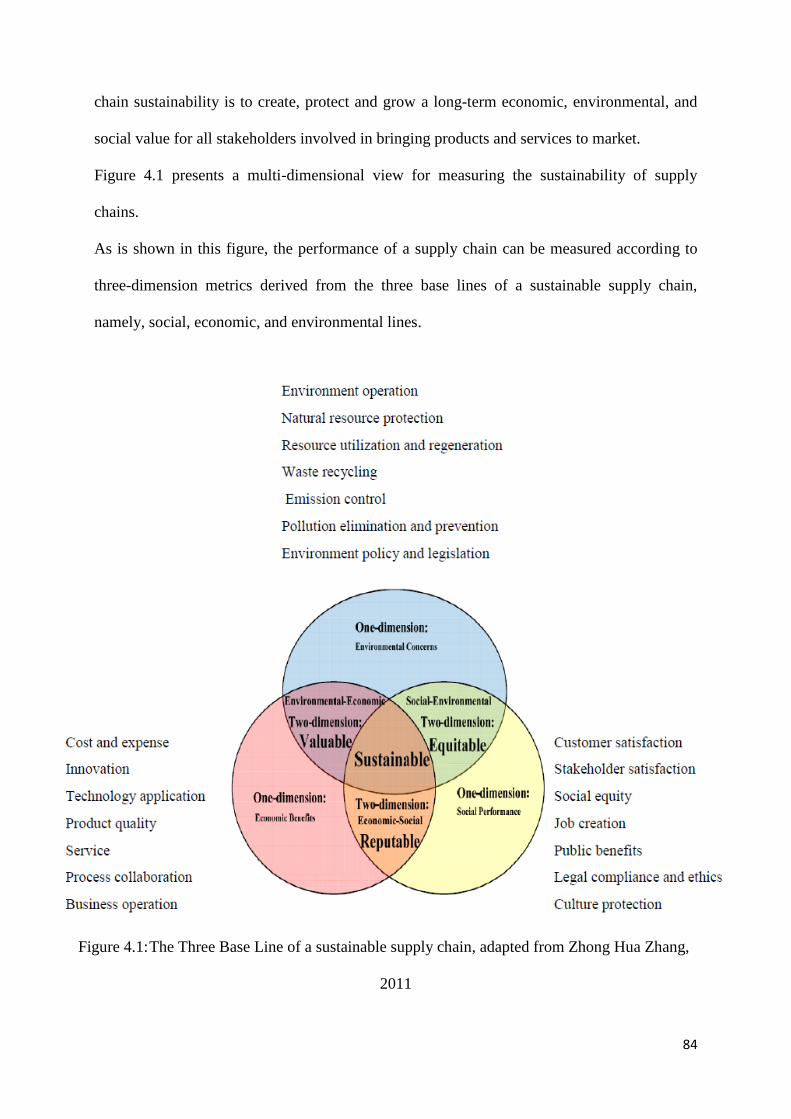
84

chain sustainability is to create, protect and grow a long-term economic, environmental, and

social value for all stakeholders involved in bringing products and services to market.

Figure 4.1 presents a multi-dimensional view for measuring the sustainability of supply

chains.

As is shown in this figure, the performance of a supply chain can be measured according to

three-dimension metrics derived from the three base lines of a sustainable supply chain,

namely, social, economic, and environmental lines.

Figure 4.1: The Three Base Line of a sustainable supply chain, adapted from Zhong Hua Zhang,

2011

85

We can talk about one-dimensional metrics, when each of the three lines is considered

individually. We may therefore be interested in either the economic dimension, or the

environmental metrics, or also the social performance of the supply chain.

A two-dimension metric is a result of each combination of two one-dimensional metrics. They

can be used to evaluate the degree of operations, processes, and activities integration in

sustainability in supply chains.

The three-dimension metrics also called as sustainable metrics, are to consider the three one-

dimensional metrics all together at a time.

A sustainable supply chain helps companies to protect the long-term viability of their product,

trying to extend the time from the launch stage until the decline stage of the product, and to

secure a social license to operate. Leading companies understand that they have a role to play

throughout the lifecycle of their products and services, and that the supply chain sustainability

is a key to maintain the integrity of a brand, ensure business continuity and manage

operational costs.

The first action in developing a supply chain sustainability strategy is to evaluate the business

case for the product and understand its external landscape. This action, formalizing the

decision to launch a new product on the market, includes several steps, such as:

4.2.1 The advisability study

This step of preliminary project, allows studying the project application and deciding if the

concept is viable. This step is to issue validating the customer‘s demand, against the overall

objectives of the organization.

This step represents eventually the base of the design of the supply chain, as it is at this stage

that the whole demand for the product is estimated, and the life cycle of the product could be

defined according to the variation in demand over time.

86

Even more, the identification of the different wholesalers and the various customer zones

should be made at the end of this study.

4.2.2 The feasibility study

This step is to analyze the economic, organizational and technical feasibility of the project.

Hence, requirements' analysis has to be done. From the summary analysis of the requirements,

it should be a rough estimate of the different costs of investment and operation of the project

(in terms of human and material resources), the expected lead-times, and the potential return

on investment. Based on these estimates, the Steering Committee may consider continuing the

project, and if necessary provide a methodological organization therefore.

This second step is also a very important one for the supply chain design. Indeed, at the end of

this step, we should have an idea about the different potential actors in the chain, in terms of

the proposed costs for raw materials, production and distribution costs, in terms of the quality

offered, the different lead-times, and even the innovation.

The collected data ,at this stage, regarding the various potential actors, will serve to evaluate

them from an economical point of view.

It is clear, therefore, that following these two steps, the project is studied from a single

perspective, namely the economical side. However, in real life, to ensure that the study was

complete and that the project will be approved by the authorities, any preliminary draft should

include a third study, namely the impact assessment study.

4.2.3 The impact assessment study

An impact study is a collective reflection which aims at assessing the consequences of all

factors, including the environmental project in an attempt to reduce, mitigate or compensate

for adverse impacts.

The awareness in the 1970s of the need to limit the damage of nature was embodied in laws

forcing to reduce noise and pollution, and to mitigate the impacts of large projects. To do so,

87

the environmental impact studies became mandatory prior to the completion of facilities or

structures, which by their size or by the importance of their impact on the natural

environment, could affect it.

In this context, the ISO 14001 standards were addressed to economic operators and

constructive business leaders to understand that the implementation of a strategic approach

can make the investments profitable, since these standards are in favor of the protection of the

environment.

Indeed, the approach of ISO 14001 requires the company to conduct a review of all the deep

areas where activities have an environmental impact.

It is an approach that has several advantages for the company. Benefits include reduced costs

of waste management, an evident energy saving, cheaper distribution costs, ...

To these advantages is added a better image of the company with the regulatory authorities

along with the international contractors, national ones, or those in the public sector. The

adoption of ISO 14001 standards allows companies to be better perceived by the agencies that

are responsible for environmental issues. The main criteria that must be analyzed on the

environmental point, are the impacts on soil, air, water, and fauna and flora (the human being

is considered). Analyzes of the impact of emissions on the atmosphere, from the chemical, the

visibility, the toxicity, or the opacity point of view, the impact of these programs on fauna and

flora, and even the study of the impact on geology, topography, hydrology, and hydrogeology.

Furthermore, the willingness of countries to meet the Kyoto Protocol goal, pushed them to

encourage manufacturers to reduce their emissions.

The Kyoto Protocol is a legally binding agreement under which industrialized countries will

reduce their collective emissions of greenhouse gases by 5.2% compared to the year 1990.

The goal is to lower the overall emissions from six greenhouse gases - carbon dioxide,

methane, nitrous oxide, sulfur hexafluoride, HFCs, and PFCs - calculated as an average over

88

the five-year period of 2008-2012. And recently, in December 2012, delegates from almost

200 countries have extended until 2020 the Kyoto Protocol for fighting climate change.

Moreover, the law on the carbon tax, which has begun to be applied in most developed

countries, discourages emissions by making polluters pay in proportion to their emissions.

This law has pushed manufacturers to be increasingly vigilant towards their carbon emissions,

and to be careful not to exceed the emission requirements, so as to minimize the tax liability

in this context.

In addition to the environmental side, this impact study could also consider the social

consequences of the project, especially when it comes to the implementations of sites. Indeed,

the consequences of these implementations are often positive for the host countries.

This could result in jobs' creation and a decrease in the unemployment rate, a transfer of

know-how and techniques, and a gradually increase of the living standards in the host

country.

If positive impacts on countries that benefit from these locations are highlighted, we must not

forget, however, the negative impact on the countries that may suffer from relocation.

Therefore, a complete understanding of the issue of relocation requires the two perspectives.

Offshoring has many social implications in countries undergoing relocations. The main

effects are the generation of layoffs and indirect job losses. They could even lead to the

bankruptcy of some subcontractors.

The more these studies are detailed and comprehensive, the more they will help design an

efficient supply chain for the product.

According to Nagurney (2009) and Chen et al. (2004), the adoption of multiple criteria and

multiple objectives in designing supply chain networks represents the system-optimization

perspective of SCN integration.

89

Indeed, after defining the product life cycle in the first advisability study, in feasibility and

impact assessment studies, a set of criteria is taken into consideration to analyze the

economical, environmental and social feasibility of the project, and to evaluate the different

potential supply chain actors.

The pinpointing of such criteria and of their importance is strongly linked to the product life

cycle and its different phases.

We can note that, at the macro-economical level, according to the marketing strategy adopted

at each product life cycle stage, the decision to establish contractual relationships with

suppliers, or to set up or to relocate production facilities or warehouses because of the lower

costs can be weakened by the consideration of structural factors such as:

- The ability to have a web of local suppliers, or producers with real guarantees of

reliability in terms of quality, time delivery, respect for commercial contracts, quality

of the services and goods produced, etc..

Indeed, the quality criterion of the product as well as the service level criterion could be very

important at the introduction stage of the product than at the other phases. While, the criterion

cost is very important at the growth and maturity stages. So, to be selected during these

stages, the supply chain actors should respond well to these criteria.

- The political and social instability in the host country, is particularly likely to make the

ways to ensure the physical security of the entity implanted too expensive.

- The state policy towards foreign investment, which, as far as possible, should not be

fluctuating; has to be verified, instead.

- The operation of the public services, the reliability of the administration (including its

level of possible corruption) and the extent of the regulatory and compliance, in

particular with regard to the right intellectual property to protect the company from the

risks of counterfeit.

90

It is instructive to observe, in this regard, that there are even re-localization phenomena,

which cause the closure of a facility and the opening of a new one. These phenomena provide

the evidence of a poor feasibility study by the company, which resulted in losses that the re-

localization is actually able to avoid. This was the case with many companies having noted

deterioration in the quality of production or services, or after some customers' complaints.

The challenging issues are how to achieve a sort of balance among the different business

goals, social concerns, and the environmental impacts of different activities in a product-

driven supply chain.

This part of the thesis focuses on the problem of designing a product-driven sustainable

supply chain network considering the (3BL) Triple Bottom Lines of maximizing economic

returns, minimizing environmental impacts, and maximizing social performance for the

supply chain. The proposed method is novel and deals with the important problem of

designing supply chain networks to achieve sustainability from a socio-economic-

environmental perspective while considering the product life cycle.

4.3 The resolution methodology:

The developed two-phase approach is based on the AHP-OWA procedure and the weighted

goal programming method, incorporating both quantitative and qualitative factors.

Thus, as in the previous chapter, the resolution procedure will be conducted in two phases

separately. The first one focuses on the performance and the effectiveness' evaluation of each

potential actor at each product life cycle stage, while the second phase focuses on the supply

chain network design. Figure 4.2 depicts the decision making process involved in the supply

chain network design. The decision maker in this framework is top executive acting as a

broker.

91

Figure 4.2: Phases for the supply chain network design

Phase I: A multi-attribute decision making problem:

The overall goal being to design a product-driven sustainable supply chain, we have three

different objectives to be optimized namely the economic, environmental, and social

objectives.

92

Each of the three objectives is broken down into a set of criteria, each of them is, in turn

decomposed into a set of sub-criteria.

This was translated into the hierarchical scheme shown in figure 4.3.

From the collected data in the beginning, following the advisability study, the feasibility study

and the impact assessment study, we can proceed to the evaluation of the potential supply

chain actors, according to the objectives, the criteria and the sub-criteria fixed by the decision

maker as well as to their correspondent importances.

As these importances vary in accordance to the product life cycle, and to the supply chain

strategy that is appropriate to each stage. An exhaustive assessment for all the potential actors

for each supply chain level separately, is then required at each stage.

Figure 4.3: Criteria hierarchy

This evaluation will be carried out by using the combination of two methods, namely the AHP

and the OWA. The above problem is solved separately for each of the three business process

types.

93

The implementation of this combination, at each product life cycle stage, involves five major

steps (See the chapter 3, section 3.4 for more details) :

(i) Developing an AHP hierarchy (figure 4.3) for each supply chain level separately, by

defining the different criteria and sub-criteria corresponding to each level.

(ii) A pair-wise comparison for all the elements of the hierarchical structure; objectives,

criteria, sub-criteria and alternatives; using the ratio scale of comparative judgments

proposed by Saaty (1980).

(iii) Specifying the linguistic quantifier Q corresponding to each criterion and to each

objective, in accordance to the supply chain strategy used at the correspondent

product life cycle stage (see chapter 3)

(iv) Generating a set of ordered weights associated with Q, and

(v) Computing the overall efficiency evaluation for each i-th alternative by means of the

OWA combination function.

This method generates an efficiency score for each candidate in each process and at each

stage. Phase I essentially identifies the candidates who will be selected for the network, by

referring to their obtained efficiency scores and to an expected efficiency average fixed by the

decision maker for each supply chain process.

This identification is formalized by efficiency constraints that will be added to the

mathematical model in the next optimization phase.

Phase II: The multi-objective supply chain network design

The existing the literature on logistics is extremely rich in terms of mathematical models that

aim at designing supply chain networks, but there are no proposed mixed integer linear

94

models that take into account both economic, environmental, and social criteria for the design

of a multi-period supply chain.

To fill in this gap, in this part of the thesis, we propose a mixed integer linear programming

model to design a sustainable multi-period and product-driven supply chain.

To ensure the supply chain sustainability, we set three objectives to be achieved.

The first one is related to the economic impact, it focuses on minimizing the supply chain

total cost.

The second objective is rather related to the supply chain environmental impact, and focuses

on minimizing the CO2 emissions across the whole chain.

And finally, because of the surrounding context of difficult economic times, we have used the

prospects for maximizing the number of job creations as the main measure of the supply chain

social impact.

Under each of these objectives, we can find a set of criteria and sub-criteria laid down by the

decision maker, and which vary according to the supply chain process.

The second phase handles the identification of actors in the chain, as well as the optimal

allocation of material from selected suppliers to manufacturers and to warehouses while still

achieving the three above cited objectives.

The model formulation

The mixed integer linear programming model developed in this section, aims at selecting

suppliers from a candidate set of suppliers, as well as to locate a given number of production

producers and distributors, subject to capacity restrictions.

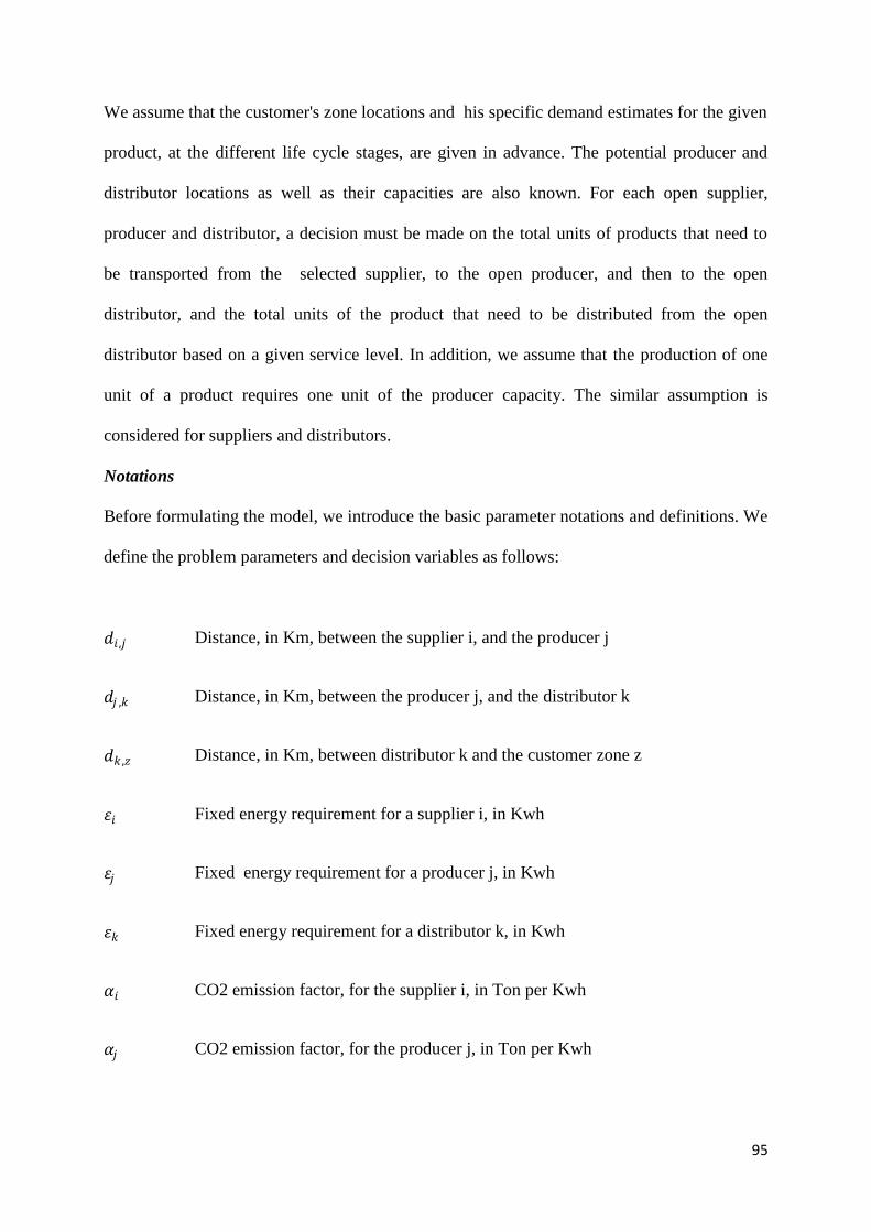
95

We assume that the customer's zone locations and his specific demand estimates for the given

product, at the different life cycle stages, are given in advance. The potential producer and

distributor locations as well as their capacities are also known. For each open supplier,

producer and distributor, a decision must be made on the total units of products that need to

be transported from the selected supplier, to the open producer, and then to the open

distributor, and the total units of the product that need to be distributed from the open

distributor based on a given service level. In addition, we assume that the production of one

unit of a product requires one unit of the producer capacity. The similar assumption is

considered for suppliers and distributors.

Notations

Before formulating the model, we introduce the basic parameter notations and definitions. We

define the problem parameters and decision variables as follows:

𝑑𝑖 ,𝑗 Distance, in Km, between the supplier i, and the producer j

𝑑𝑗 ,𝑘 Distance, in Km, between the producer j, and the distributor k

𝑑𝑘 ,𝑧 Distance, in Km, between distributor k and the customer zone z

𝜀𝑖 Fixed energy requirement for a supplier i, in Kwh

𝜀𝑗 Fixed energy requirement for a producer j, in Kwh

𝜀𝑘 Fixed energy requirement for a distributor k, in Kwh

𝛼𝑖 CO2 emission factor, for the supplier i, in Ton per Kwh

𝛼𝑗 CO2 emission factor, for the producer j, in Ton per Kwh

96

𝛼𝑘 CO2 emission factor, for the distributor k, in Ton per Kwh

𝛼𝑠 CO2 emission factor for transportation, in Ton per Ton.Km

𝐽𝐶𝑖 ,𝑡 Number of jobs created due to the opening of the supplier i at stage t

𝐽𝐶𝑗 ,𝑡 Number of jobs created due to the opening of the producer j at stage t

𝐽𝐶𝑘 ,𝑡 Number of jobs created due to the opening of the distributor k at stage t

The remaining model parameters and decision variables are the same used in chapter 3, in

section 3.5.

We suppose that the fixed costs of the closing sites include, as the case may show, either the

economic redundancy allowance for employees following a permanent closure of the site or a

temporary one if there's a possible reopening later.

As mentioned before, our model has three objectives: to minimize the supply chain total cost,

to minimize the total CO2 emissions, and to maximize the number of created jobs throughout


The total cost of the supply chain includes the fixed opening and closing of the sites, the fixed

costs to operate each of these sites, purchasing costs, production costs, transportation and

distribution cost. Therefore, the objective function to be minimized is given by:

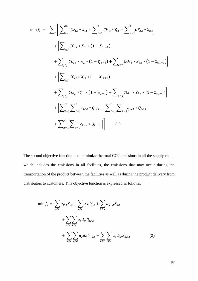
97

min 𝑓1 = 𝐶𝐹𝑖 ,𝑡 ∗ 𝑋𝑖,𝑡 + 𝐶𝐹𝑗 ,𝑡 ∗ 𝑌𝑗 ,𝑡 + 𝐶𝐹𝑘 ,𝑡

𝑝

𝑘=1

𝑛

𝑗=1

𝑚


𝑡

+ 𝐶𝑂𝑖,𝑡 ∗ 𝑋𝑖,𝑡 ∗ 1 − 𝑋𝑖 ,𝑡−1 𝑖∈𝐼


∗ 𝑍𝑘 ,𝑡 ∗ 1 − 𝑍𝑘 ,𝑡−1

+ 𝐶𝐶𝑖 ,𝑡 ∗ 𝑋𝑖 ,𝑡 ∗ 1 − 𝑋𝑖,𝑡+1 𝑖∈𝐼


∗ 𝑍𝑘 ,𝑡 ∗ (1 − 𝑍𝑘 ,𝑡+1)

+ 𝑐𝑖 ,𝑗 ,𝑡 ∗ 𝑄𝑖,𝑗 ,𝑡 + 𝑐𝑗 ,𝑘 ,𝑡 ∗ 𝑄𝑗 ,𝑘 ,𝑡

𝑝

𝑘=1

𝑛

𝑗=1

𝑛

𝑗=1

𝑚

𝑖=1

+ 𝑐𝑘 ,𝑧,𝑡 ∗ 𝑄𝑘 ,𝑧 ,𝑡 𝑞

𝑧=1

𝑝

𝑘=1 (1)

The second objective function is to minimize the total CO2 emissions in all the supply chain,

which includes the emissions in all facilities, the emissions that may occur during the

transportation of the product between the facilities as well as during the product delivery from

distributors to customers. This objective function is expressed as follows:

min 𝑓2 = 𝛼𝑖𝜀𝑖𝑋𝑖,𝑡 + 𝛼𝑗 𝜀𝑗𝑌𝑗 ,𝑡

𝑗∈𝐽𝑖∈𝐼

+ 𝛼𝑘𝜀𝑘𝑍𝑘 ,𝑡

𝑘∈𝐾

+ 𝛼𝑠𝑑𝑖𝑗𝑄𝑖 ,𝑗 ,𝑡

𝑗∈𝐽𝑖∈𝐼

+ 𝛼𝑠𝑑𝑗𝑘 𝑌𝑗 ,𝑘 ,𝑡 + 𝛼𝑠𝑑𝑘𝑧𝑍𝑘 ,𝑧,𝑡 (2)

𝑧∈𝑍𝑘∈𝐾𝑘∈𝐾𝑗∈𝐽

98

And finally, the third objective that maximizes the job creations is represented as follows:

max 𝑓3 = 𝐽𝐶𝑖 ,𝑡 ∗ 𝑋𝑖 ,𝑡 ∗ 1 − 𝑋𝑖,𝑡−1 𝑖∈𝐼𝑡

+ 𝐽𝐶𝑗 ,𝑡 ∗ 𝑌𝑗 ,𝑡 ∗ 1 − 𝑌𝑗 ,𝑡−1 + 𝐽𝐶𝑘 ,𝑡𝑘∈𝐾𝑗∈𝐽

∗ 𝑍𝑘 ,𝑡 ∗ 1 − 𝑍𝑘 ,𝑡−1 3

s.t


𝑒𝑖 ,𝑡𝑋𝑖,𝑡 ≥ 𝐸𝑒𝑥𝑝𝐼,𝑡 𝑋𝑖,𝑡 ∀ 𝑖, 𝑡 (4)

𝑒𝑗 ,𝑡𝑌𝑗 ,𝑡 ≥ 𝐸𝑒𝑥𝑝𝐽 ,𝑡 𝑌𝑗 ,𝑡 ∀ 𝑗, 𝑡 (5)

𝑒𝑘 ,𝑡𝑍𝑗 ,𝑡 ≥ 𝐸𝑒𝑥𝑝𝐾,𝑡 𝑍𝑘 ,𝑡 ∀ 𝑘, 𝑡 (6)


𝑋𝑖 ,𝑗 ,𝑡 ≤ 𝑐𝑎𝑝𝑖 ,𝑡 ∗ 𝑋𝑖 ,𝑡 ∀ 𝑖𝑛

𝑗=1, 𝑡

(7)

𝑌𝑗 ,𝑘 ,𝑡 ≤ 𝑐𝑎𝑝𝑗 ,𝑡 ∗ 𝑌𝑗 ,𝑡 ∀𝑗𝑝

𝑘=1, 𝑡

(8)

𝑍𝑘 ,𝑧 ,𝑡 ≤ 𝑐𝑎𝑝𝑘 ,𝑡 ∗ 𝑍𝑘 ,𝑡 ∀𝑘𝑞

𝑧=1, 𝑡

(9)


𝑋𝑄𝑖,𝑗 ,𝑡 − 𝑄𝑗 ,𝑘 ,𝑡 = 0 ∀ 𝑗 , 𝑡 𝑝

𝑘=1

𝑚

𝑖=1

(10)


𝑞

𝑧=1= 0 ∀ 𝑘 , 𝑡

𝑛

𝑗=1

(11)



𝑘=1

(12)

99


𝑄𝑖 ,𝑗 ,𝑡 ≥ 0 ∀ 𝑖, 𝑗 , 𝑡 (13)

𝑄𝑗 ,𝑘 ,𝑡 ≥ 0 ∀ 𝑗, 𝑘, 𝑡 (14)

𝑄𝑘 ,𝑧 ,𝑡 ≥ 0 ∀ 𝑘, 𝑧, 𝑡 (15)

𝑋𝑖,𝑡 ∈ 0,1 ∀𝑖, 𝑡 (16)

𝑌𝑗 ,𝑡 ∈ 0,1 ∀𝑗, 𝑡 (17)

𝑍𝑘 ,𝑡 ∈ 0,1 ∀𝑘, 𝑡 (18)

𝑖 = 1, … , 𝑚,

𝑗 = 1, … , 𝑛,

𝑘 = 1, … , 𝑝,

𝑧 = 1, … , 𝑞

The model reformulation

To linearize the economic and the social objective functions, (1) and (3), we use the same

linearization technique as proposed by Fortet (1959),and that we have already detailed in the

previous chapter and which involves replacing each product of two binary variables by a

single additional variable and two auxiliary linear constraints.

Therefore, the economic function is rewritten as:

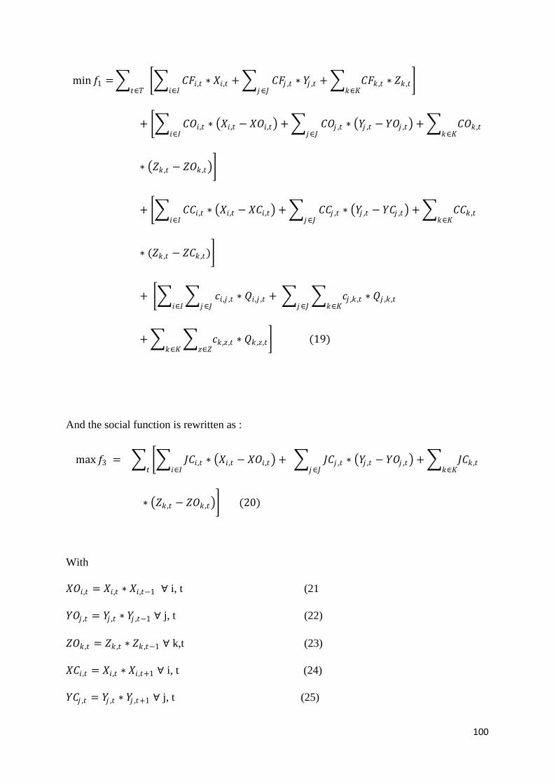
100

min 𝑓1 = 𝐶𝐹𝑖 ,𝑡 ∗ 𝑋𝑖,𝑡 + 𝐶𝐹𝑗 ,𝑡 ∗ 𝑌𝑗 ,𝑡 + 𝐶𝐹𝑘 ,𝑡𝑘∈𝐾𝑗∈𝐽𝑖∈𝐼





∗ (𝑍𝑘 ,𝑡 − 𝑍𝐶𝑘 ,𝑡)



(19)

And the social function is rewritten as :

max 𝑓3 = 𝐽𝐶𝑖 ,𝑡 ∗ 𝑋𝑖,𝑡 − 𝑋𝑂𝑖,𝑡 + 𝐽𝐶𝑗 ,𝑡 ∗ 𝑌𝑗 ,𝑡 − 𝑌𝑂𝑗 ,𝑡 + 𝐽𝐶𝑘 ,𝑡𝑘∈𝐾𝑗∈𝐽𝑖∈𝐼𝑡

∗ 𝑍𝑘 ,𝑡 − 𝑍𝑂𝑘 ,𝑡 (20)

With

𝑋𝑂𝑖,𝑡 = 𝑋𝑖,𝑡 ∗ 𝑋𝑖,𝑡−1 ∀ i, t (21

𝑌𝑂𝑗 ,𝑡 = 𝑌𝑗 ,𝑡 ∗ 𝑌𝑗 ,𝑡−1 ∀ j, t (22)

𝑍𝑂𝑘 ,𝑡 = 𝑍𝑘 ,𝑡 ∗ 𝑍𝑘 ,𝑡−1 ∀ k,t (23)

𝑋𝐶𝑖 ,𝑡 = 𝑋𝑖,𝑡 ∗ 𝑋𝑖 ,𝑡+1 ∀ i, t (24)

𝑌𝐶𝑗 ,𝑡 = 𝑌𝑗 ,𝑡 ∗ 𝑌𝑗 ,𝑡+1 ∀ j, t (25)

101

𝑍𝐶𝑘 ,𝑡 = 𝑍𝑘 ,𝑡 ∗ 𝑍𝑘 ,𝑡+1 ∀ k, t (26)

For linearization, the following constraints are added to the previous problem constraints:

Linearization constraints

To solve the proposed mathematical model, and satisfies the three goals, a weighted goal

programming technique is applied.

𝑋𝑂𝑖,𝑡 ≤ 𝑋𝑖 ,𝑡 ∀ 𝑖 (27)

𝑌𝑂𝑗 ,𝑡 ≤ 𝑌𝑗 ,𝑡 ∀ 𝑗 (28)

𝑍𝑂𝑘 ,𝑡 ≤ 𝑍𝑘 ,𝑡 ∀ 𝑘 (29)

𝑋𝑂𝑖,𝑡 ≤ 𝑋𝑖 ,𝑡−1 ∀ 𝑖 (30)

𝑌𝑂𝑗 ,𝑡 ≤ 𝑌𝑗 ,𝑡−1 ∀ 𝑗 (31)

𝑍𝑂𝑘 ,𝑡 ≤ 𝑍𝑘 ,𝑡−1 ∀ 𝑘 (32)

𝑋𝑂𝑖,𝑡 ≥ 𝑋𝑖 ,𝑡 + 𝑋𝑖,𝑡−1 − 1 ∀ 𝑖 (33)

𝑌𝑂𝑖 ,𝑡 ≥ 𝑌𝑖 ,𝑡 + 𝑌𝑖 ,𝑡−1 − 1 ∀ 𝑗 (34)

𝑍𝑂𝑖,𝑡 ≥ 𝑍𝑖 ,𝑡 + 𝑍𝑖 ,𝑡−1 − 1 ∀ 𝑘 (35)

𝑋𝐶𝑖 ,𝑡 ≤ 𝑋𝑖,𝑡 ∀ 𝑖 (36)

𝑌𝐶𝑗 ,𝑡 ≤ 𝑌𝑗 ,𝑡 ∀ 𝑗 (37)

𝑍𝐶𝑘 ,𝑡 ≤ 𝑍𝑘 ,𝑡 ∀ 𝑘 (38)

𝑋𝐶𝑖 ,𝑡 ≤ 𝑋𝑖,𝑡−1 ∀ 𝑖 (39)

𝑌𝐶𝑗 ,𝑡 ≤ 𝑌𝑗 ,𝑡−1 ∀ 𝑗 (40)

𝑍𝐶𝑘 ,𝑡 ≤ 𝑍𝑘 ,𝑡−1 ∀ 𝑘 (41)

𝑋𝐶𝑗 ,𝑡 ≥ 𝑋𝑖,𝑡 + 𝑋𝑖,𝑡−1 − 1 ∀ 𝑖 (42)

𝑌𝐶𝑗 ,𝑡 ≥ 𝑌𝑗 ,𝑡 + 𝑌𝑗 ,𝑡−1 − 1 ∀ 𝑗 (43)

𝑍𝐶𝑘 ,𝑡 ≥ 𝑍𝑘 ,𝑡 + 𝑍𝑘 ,𝑡−1 − 1 ∀ 𝑘 (44)

102

The weighted goal programming technique

The roots of the goal programming technique lie in a paper by Charnes et al. (1955) in which

they deal with the executive compensation methods. A more explicit definition is given by

Charnes and Cooper (1961) in which the term ―goal programming‖ is first used.

The goal programming is an important technique for allowing the decision makers to consider

several objectives in finding a set of acceptable solutions. It has been accomplished with

various methods such as Lexicographic (Preemptive), Weight (Archimedean), and MINIMAX

(Chebyshev) achievement functions (Romero, 2004).

It can also be said that the goal programming has been, and still is, the most widely used

technique for solving multi-criteria decision-making problems (Romero, 2004).

In general, the purpose of this technique is to minimize the deviation between the

achievements of goals and their acceptable aspiration levels.

It is a special compromise multi-criteria method assuming that the decision maker knows

goals‘ values and their relative importance (Liu, 2008). It is designed to consider many goals

simultaneously when searching for a compromise solution and is supported by a mathematical

programming optimization potential (Martel and Aouni, 1998). Applied philosophy of

compromise solution searching defines a variety of goal programming techniques (Jones and

Tamiz, 2010). Each type of achievement function utilized leads to different goal programming

variants. In this chapter, weighted goal programming (WGP) will be applied.

WGP is resting on Archimedean achievement function minimizing the sum of weighted

deviations from target values. They are measured using positive and negative deviational

variables defined for each goal separately, presenting either over- or underachievement of the

103

goal. Negative deviation variables are included in the objective function for goals that are of

the type ‗more is better‘, and positive deviation variables are included in the objective

function for goals of the type ‗less is better‘. Since any deviation is undesired, the relative

importance of each deviation variable is determined by associated weights, reflecting decision

maker‘s preferences among goals. For the objective function, it is typical that it minimizes

undesirable deviations from the target goal levels and does not minimize or maximize the

goals themselves (Ferguson et al., 2006).

The algebraic formulation of a WGP is given as:

min 𝑔 = 𝑢𝑞𝑛𝑞 + 𝑣𝑞𝑝𝑞

𝑄

𝑞=1

s.t

𝑓𝑞 𝑥 + 𝑛𝑞 − 𝑝𝑞 = 𝑏𝑞 𝑞 = 1, … , 𝑄

𝑥 ∈ 𝐹

𝑛𝑞 , 𝑝𝑞 ≥ 0 (34)

Where 𝑓𝑞 𝑥 is a linear function of x, and 𝑏𝑞 the target value for that objective. 𝑛𝑞 and 𝑝𝑞

represent the negative and positive deviations from this target value. 𝑢𝑞 and 𝑣𝑞 are the

respective positive weights attached to these deviations in the achievement function 𝑔.

These weights take the value zero if the minimization of the corresponding deviational

variable is not important to the decision maker. 𝐹 is an optional set of hard constraints as

found in linear programming.

In addition, a major issue of debate within the GP community has concerned the use of

normalization techniques to overcome incommensurability. Incommensurability in a WGP

occurs when deviational variables measured in different units are summed up directly, as is

the case for the proposed mathematical model in this chapter.

104

This simple summation will cause an unintentional bias towards the objectives with a larger

magnitude. This bias may lead to erroneous or misleading results.

One suggestion to overcome this difficulty is to divide each objective through by a constant

pertaining to that objective. This ensures that all objectives have roughly the same magnitude.

Such a constant is known as normalization constant. This leads to the revised algebraic format

for a WGP:

min 𝑔 = 𝑢𝑞𝑛𝑞

𝑘𝑞+

𝑣𝑞𝑝𝑞

𝑘𝑞

𝑄

𝑞=1

s.t

𝑓𝑞 𝑥 + 𝑛𝑞 − 𝑝𝑞 = 𝑏𝑞 𝑞 = 1, … , 𝑄

𝑥 ∈ 𝐹

𝑛𝑞 , 𝑝𝑞 ≥ 0 (35)

where 𝑘𝑞 is the normalization constant for the q-th objective.

Within WGP, all deviations are expressed as a ratio difference (i.e., (desired – actual)/desired)

= (deviation)/desired)). In this case, any marginal change within one observed goal is of equal

importance, no matter how distant it is from target value (Rehman and Romero 1987).

The model is then formulated as follows:

min 𝑢1𝑝1

𝑘1 +

𝑢2𝑝2

𝑘2 +

𝑣3𝑛3

𝑘3 (36)

s.t

(4) - (18)

(21) - (33)

𝑓1 − 𝑝1 + 𝑛1 = 𝑏1 (37)

105

𝑓2 − 𝑝2 + 𝑛2 = 𝑏2 (38)

𝑓3 − 𝑝3 + 𝑛3 = 𝑏3 (39)

𝑛𝑞 , 𝑝𝑞 ≥ 0 ∀ 𝑞 = 1,2,3 (40)

Where

4.4 Numerical example

This section presents a small-scale supply chain design problem adapted from a real-life

situation. The purpose is neither to show any advantage of the modeling process by

comparing it with other MIP models, nor to exhibit the efficiency of problem solving by

benchmarking the computation time to other algorithms. Indeed, we aim at illustrating the

effectiveness and convenience of the product life cycle consideration in the sustainable supply

chain design, by introducing a multi-criteria decision making and multi-objective models to

select the effective supply chain actors in the different product life cycles' stages.

We consider the case of a focal company which is on the edge of the launching process of a

new product on the market, namely, the environmentally coal from the olive pomace. The

𝑢1 Weight of the economical objective determined using the AHP in the phase 1

𝑢2 Weight of the environmental objective determined using the AHP in the phase 1

𝑣3 Weight of the social objective determined using the AHP in the phase 1

𝑘1 Normalizing constant for the objective 1



𝑏1 Target value for the objective 1



106

company has to design a sustainable supply chain with a minimal cost, minimal CO2

emissions and maximal jobs made available, considering the product life cycle stages.

The multiple attribute matrices and the efficiency scores for the introduction and maturity

phases, obtained from phase I, are shown in tables 4.1, 4.2 and 4.3, for the suppliers,

producers and distributors respectively. The last line in each table represents the efficiency

scores of the potential actors at the corresponding product life cycle stage.

The mathematical model is then solved to identify the optimum supply chain network.

Figure 4.4 shows the sales' distribution in Ton for the 3 different customer zones.

Fixing the target levels to 𝑓1∗ , 𝑓2

∗ and 𝑓3∗; the optimal solution values of the mono-objective

problem under 𝑓1 , 𝑓2 and 𝑓3 respectively. Table 4.4 illustrates the optimal deployment plans

for the supply chain network for the four different stages of the product life cycle. The

optimal supply chain actors and the number of units to be shipped from each source to each

destination are clearly depicted in this transshipment solution.

In this table, we can clearly remark the change of the network and the flows from one phase to

another, but this change could be due to the variation of two factors, namely the demand, and

the efficiency scores of the different actors.

To better see the contribution of the first phase of this model, we solved the same problem

again, but by maintaining the same demand data for the four product life cycle stages.

Table 4.5 and 4.6 show the optimal deployment plans for the supply chain network for the

introduction and the maturity phases, respectively.

107

Table 4.1: Multiple attribute matrix on supply performance and efficiency scores

108

Table 4.2: Multiple attribute matrix on production performance and efficiency scores

109

Table 4.3: Multiple attribute matrix on distribution performance and efficiency scores

110

Figure 4.4: Sales distribution of the product in Ton

Table 4.4: The optimal supply chain network

Table 4.5: Optimal supply chain network for the introduction stage

Introducion stage P1 D2 Z1 Z2 Z3

S3 16000

P1 16000

D2 8000 3500 2500

Demand >=8000 >=3500 >=4500

111

Table 4.6: Optimal supply chain network for the introduction stage

Maturity stage P1 D3 Z1 Z2 Z3

S2 16000

P1 16000

D3 8000 3500 4500

Demand >=8000 >=3500 >=4500

Comparing the two tables 4.5 and 4.6, we can infer that the proposed approach cannot only

adopt the supply chain strategy according to the degree of concern at different phases, but also

consider the trade-off effect to avoid selecting inefficient actors in the correspondent product

life cycle stage.

From the results listed in table 4.6 for the maturity phase, it is interesting to notice that

supplier 2, who was considered to be inefficient in the introduction phase, was selected as an

efficient actor in the maturity phase, and similarly for the distributor 3.

4.5 Sensitivity analysis

We examined the sensitivity of the supply chain performance due to a variation in the

objective weights' values. Figure 4.5 shows the goals satisfaction levels of the whole supply

chain from the introduction to the decline phase of the product life cycle.

From the results shown in this figure, we realize that, apart from the three special cases where

we have considered a single objective at a time, the three objectives are almost fully achieved.

Indeed, we could remark that, in the worst cases, the economical objective was achieved to

80%, while the environmental and the social objectives were achieved to 86% and 55%,

respectively.

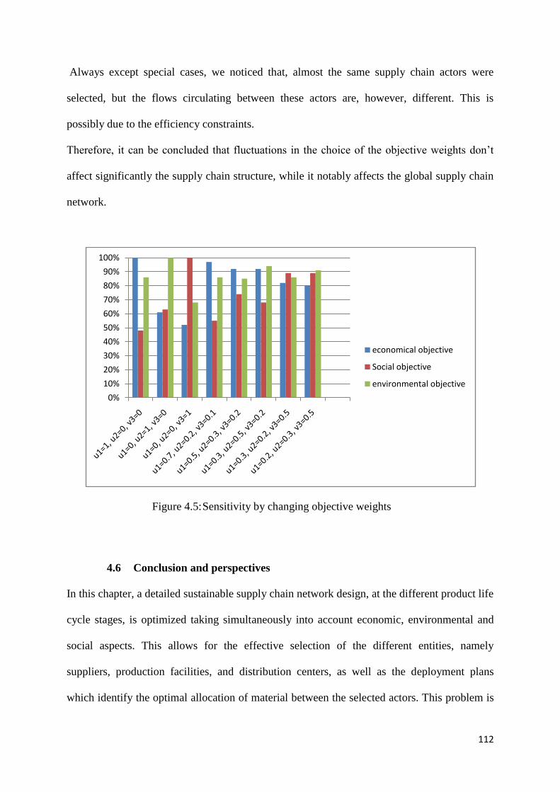
112

Always except special cases, we noticed that, almost the same supply chain actors were

selected, but the flows circulating between these actors are, however, different. This is

possibly due to the efficiency constraints.

Therefore, it can be concluded that fluctuations in the choice of the objective weights don‘t

affect significantly the supply chain structure, while it notably affects the global supply chain

network.

Figure 4.5: Sensitivity by changing objective weights

4.6 Conclusion and perspectives

In this chapter, a detailed sustainable supply chain network design, at the different product life

cycle stages, is optimized taking simultaneously into account economic, environmental and

social aspects. This allows for the effective selection of the different entities, namely

suppliers, production facilities, and distribution centers, as well as the deployment plans

which identify the optimal allocation of material between the selected actors. This problem is

0%

10%

20%

30%

40%

50%

60%

70%

80%

90%

100%

economical objective

Social objective

environmental objective

113

modeled as a multi-objective optimization problem and resolved using the weighted goal

programming approach.

The case of production and delivery of multiple products that are in different product life

cycle stages is another interesting issue that needs to be considered.

114

5.1 Introduction

In the previous chapters, we have assumed that the product has a classical life cycle.

However, in the reality this is not always the case. Indeed, some products have very atypical

life cycles, whose curves are very different from the classical one.

To tackle this problem, in this chapter, we propose a stochastic model to design a robust

supply chain network, taking into account the different product life cycle scenarios.

The idea of the life cycle of a product is commonly used by the marketing professionals, this

explains the presence of extensive researches focusing on this theory in the marketing the

literature.

Indeed, each product follows its own life cycle, characterized by four phases: initiation,

growth, maturity, and decline. The respective durations of these phases, as well as that of the

total life cycle are highly variable depending on the products, and each phase is characterized

by its growth rate, sales' volume, profitability, and adopted marketing strategies. In many

CHAPTER 5

A Supply chain design under product life cycle

uncertainty

115

situations, it is difficult to accurately determine the life cycle of a product. This depends on

both the product and the market in which it is commercialized.

The concept of life cycle is not to be called into question. In contrast, its representation, by the

classical curve is not always true. Indeed, many products have very different curves, as shown

in figure 5.1.

After the introduction phase, some products have difficulty in finding buyers, and therefore

they experience a failure since the launching phase, and move directly to the decline phase.

Other products may experience a very rapid adoption, but consumers also grow weary very

quickly. The product in this case does not reach the maturity phase, and goes directly to the

decline phase. These phases can also be lengthened or shortened.

In this chapter, the main question is: How to take into account the product life cycle

uncertainty on the supply chain design? To address this issue, a strategic stochastic

programming based model is proposed. Such a stochastic model seeks a solution which is

appropriately balanced between some alternative product life cycle scenarios identified by

field experts.

This chapter is structured as follows: the next section will present the main topic of this

chapter. Subsequently, we present the proposed two-stage mathematical model, and indicate

how the deterministic model may be extended using stochastic programming techniques,

according to the available information on the uncertain factors. A test problem is solved, and

the results of the stochastic programming and the deterministic approaches are presented in

section 4. Finally, a conclusion and directions for future researches are presented.

116

5.2 The main topic

The life cycle theory has been extensively used in marketing. The PLC is the most well-

known one, in which the time horizon is divided into four stages based on the variation on the

overall sales' level.

Theoretically, the product life cycle should begin with the introductory stage, then growth,

maturity and finally the decline stage.

According to the marketing researches, unit sales are low in introduction, because few

consumers are attentive to the product.

With consumers' awareness and appreciation, unit sales begin to raise at an increasing rate.

This heralds the beginning of the growth stage.

After a while, unit sales attain a plateau, and the product is in the maturity stage. The majority

of the mass-market has lastly procured the product. As consumers gradually leave the product

for its most recent counterparts, unit sales will decrease immediately. Thus, the withdrawal of

the product from the market becomes imminent.

Anyhow, this scenario remains the most classical.

In fact, since the introduction of the idea of the PLC, numerous managerial-oriented articles

and book have discussed this theory, and they all reached agreement on the fact that there may

be a variety of life cycle curves, that could be different from the classical one.

The classical PLC shape, that we used previously, was only one of 12 types of PLC patterns

discovered by investigators. In figure 5.1, we can distinguish these 12 different curves.

The researches that led to these different patterns shown in figure 1 have been quite different.

According to Rink and Swan (1979), about 15 of different studies of consumer nondurables

and durables, as well as four studies of industrial goods, have shown that some products have

indeed validated the classical PLC curve.

117

However, it is very important to define the life cycle curve since the early stage, prior to the

SC design, as the PLC directs the supply chain to the appropriate market strategy in each

stage. Appropriate strategies, such as pricing, promotions, model changes, distribution

channels, service level, and others, are different according to the stages.

118

Figure 5.1: The different PLC curves, adapted from Rink and Swan (1979)

119

a Adapted from Cox [34]

b Adapted from Buzell [20]

c Adapted from Headen [55]

d Adapted from Fzederixion [46]

e Adapted from Buzzell and Nourse [19]

f Adapted from Hinkle [59]

The introductory stage is a period of a moderate growth since the new product is gradually

introduced to the market. During this stage, the first customers are still pioneers, and

competition is supported. The costs involved in the launch (commercial expenses,

technological, marketing ...) are often higher than the benefits. So, the sales of very common

products today such as DVD, have stagnated for a period and had a difficult start before to be

developed. Advertising expenses must be important, to inform consumers and encourage them

to buy the product and also to ensure the distribution of the product to the maximum number

of retailers. Indeed, the more a product is distributed, the more it will be visible by the

consumer and therefore the results will be better in its introductory stage.

The growth stage is characterized by an increase in sales of the product through word to

mouth favorable to bring new customers. New competitors are also entering the market,

attracted by the possibilities of development (which may even be beneficial for the product).

During this phase, growth should be supported as long as possible by improving the product's

quality, expanding its assortment to reach more customers, continuing communication

campaigns and lowering gradually the prices.

Also, the distribution channels have to be boosted to be able to respond much easier and

quicker to the expansion of customer needs.

120

The maturity phase is longer than the two previous phases, and is characterized by a

slowdown of the product's sales. In addition to that, competition is sharper than that in the

previous phases, and the company must reduce its prices. In the maturity phase, creativity is

needed in order to keep old customers and attract new ones, and the marketing manager must

extend the market by entering new segments, and modify the product by adding new features

to boost sales.

The decline phase is characterized by a collapse in sales. This stage is generally due to several

factors, including the technological breakthroughs, the changes in tastes or habits, or also the

arrival of cheaper foreign products. The company may decide either to withdraw from the

market or to keep the product on the market. The marketing manager must boost sales of the

product by investing in modernizing the product, and seeking how to retain its customers.

Since a supply chain is dynamic and chaotic, it should be able to easily adapt its different

partners in order to get a competitive advantage. Certainly, the supply chain structure must be

very robust to deal with the unpredictable market demand, the uncompromising levels of

competition, and the different product life cycle patterns.

As uncertainty is one of the characteristics of product-driven supply chain networks, the

strategic phase has to take into account uncertain information.

In this chapter, we present a stochastic programming based method that seeks a solution

which is appropriately balanced between some alternative product life cycle scenarios,

identified by field experts. We apply the stochastic models to a representative real case study.

The interpretation of the results will give more insight into decision-making under uncertainty

for the supply chain design.

121

Since the aim is to develop insights for problems with real-world dimensions, the construction

of the stochastic models deliberately follows a rather simple technique, which may be

potentially used to extend, in a reasonable manner, any large supply chain design model in

which uncertainty is an issue and a relatively small set of realistic scenarios can be identified.

5.3 Problem statement

Further to the launching of a new product on the market, a company has to design its

supply chain for a fixed horizon time H, so as to minimize its total cost while considering the

product life cycle uncertainty. To meet this objective, we propose a stochastic mathematical

model.

This model aims at selecting, for whatever scenario, a set of suppliers to provide a given

number of plants already located to supply a collection of distributor centers. In turn, the

selected distributors supply a set of wholesalers with specified demand quantities of the

product, so as to minimize the supply chain total cost.

As mentioned, the case at hand concerns the design of a multi-level supply chain network in

which suppliers, manufacturers, and distribution tasks are to be selected across a set of

potential ones.

In the model set-up for this problem, we use as an objective function the supply chain design

total costs.

These costs are fixed costs for processing, opening or closing the facilities, as well as variable

purchasing, manufacturing and distributing costs based on amounts of product processed and

respectively shipped between sites. The objective function is determined for the whole

product life cycle.

122

Consequently fixed costs for opening or closing the facilities vary from one site to another,

over the planning horizon. Processing costs depends only on the type of facility.

The distribution costs are supposed to be proportional to the amount and the distance over

which it is transported. The transportation costs of the product between the different actors are

assumed to be CIF costs (including Cost, Insurance, and Freight).

The underlying model can be verbally described as:

Minimize the sum over the product life cycle stages of the total supply chain costs =

Sum of (fixed processing costs + fixed opening costs + fixed closing costs) +

Sum of (purchasing materials costs + production costs + distribution costs).

Subject to:

1. Supplier‘s capacity limits,

2. Production capacity limits of the plants,

3. Distributor‘s capacity limits,

4. Market total demand satisfaction,

5. Flow conservation constraints,

The stochastic extensions proposed below, further concentrate on finding the appropriate

supply chain actors. The focus on the supply chain design issue is motivated by the fact that

investments are made on long run and are based on uncertain information. Since these

networks are expensive and difficult to change, establishing a more robust design for the

supply chain network becomes a central issue at stake. Therefore the models are primarily

configured with a variable infrastructure to assess who are the actors to be selected, but they

123

can be configured as well with all the fixed infrastructure to investigate operational aspects of

candidate network configurations.

5.4 Data and uncertainty

Especially when uncertainties are involved, a thorough data analysis, related to the

distribution of sales and to the specifications of the product life cycle stages, is needed before

going into the actual modeling phase. Among others, such an analysis should establish the

relations between the possible actors' capacities and the assumed range of supply levels, as

well as the relations between the most likely levels of supply and demand.

The scenario generation has important implications at two levels of discussion. Generally, the

outcomes of any scenario-based method will depend on the input, which in turn will rely on

the experience and guidance of domain experts. It is therefore necessary that those authorities

identify critical scenarios and that the results are carefully interpreted relative to the scenario

definition. However, within any established scenario scheme, more robustness is expected to

be achieved by accounting for multiple alternatives than just for one or few possibilities.

This is a necessary priori analysis of the data, in order to achieve an effective model. In

general, if given one or more capacities, multiple supply levels are deemed relevant, clearly

all the corresponding scenarios should be accounted for. Moreover, if probabilities were to be

associated with them in a non-symmetric distribution, this would be one more reason not to

use only its end point values.

5.5 The stochastic programming approach

Define Ω as the set of all possible scenarios and 𝜔 ∈ Ω as a particular scenario. In order to

describe the main ideas of the stochastic approach, we use here a brief notation for the

deterministic model: all the integer decision variables are included into one vector y of

124

dimension m and all the continuous decision variables are included into one vector x of

dimension n. The notation for the coefficients is adjusted accordingly: f is the m-dimensional

vector of the fixed costs for opening facilities and c is the vector of dimension n containing

the rest of the coefficients in the objective function. Then the concise deterministic model for

scenario 𝜔 can be stated as:

min 𝑓𝑦 + 𝑐 𝜔 𝑥

S/t

𝑊0 𝜔 𝑥 ≥ 0

𝑇𝑦 − 𝑊1 𝜔 𝑥 ≥ 0

𝑊2 𝜔 𝑥 − 𝑊3 𝜔 𝑥 = 0

𝑊4 𝜔 𝑥 ≥ 𝑑 𝜔

𝑦 ∈ 0, 1 𝑚

𝑥 ∈ 𝑅𝑛

𝑥 ≥ 0

The four constraint types represent the efficiency constraints, the capacity constraints, the

flow conservation constraints, and the market demand satisfaction constraint respectively.

In a stochastic programming approach, probabilities are associated with scenarios and a

solution is sought which is suitably balanced against the various scenarios (see Birge and

Louveaux, 1997; Kall and Wallace, 1994). The stochastic solution is not optimal in general

for any of the individual scenarios. In a context as considered here, the probabilities assigned

to scenarios are of subjective nature. They can be as well called weights and seen as reflecting

a relative importance in an uncertain environment. However, passing to a probabilistic

framework provides a convenient scheme for organizing ideas that mathematically fall into

125

the same patterns. Although subjective in nature, such probability specifications can support a

meaningful sensitivity analysis and guide the selection of an appropriate configuration.

Generally, a stochastic programming approach searches a solution relative to an assumed

probabilistic data structure, which may or may not reflect accurately the reality at a later

moment, but should reflect as accurate as possible the available information for present

decisions. We use such an approach in the sequel to address specific questions about the

impact of the product life cycle uncertainty on the network design.

5.6 Uncertainty on Product life cycle

Define Ω as the set of all possible product life cycle scenarios and 𝜔 ∈ Ω as a particular

scenario. Only the right hand side parameter d is determined to change in demand for each

scenario. In order to approach this uncertainty, we extend the deterministic model above to

the following two-stage stochastic model: the first stage corresponds to the investments that

must be made for opening facilities prior to knowing the actual realizations of the random

parameters and the second stage corresponds to the allocation of flows through the established

network after the values of the random parameters become known. Consequently the location

variables y are assigned as first stage variables and the allocation variables x are assigned as

second stage variables. For each pair (y, x) ,the performance measure is given by the second

stage program as the minimum total cost that can be achieved in the network given by

location y and under scenario x. The decision y is evaluated by this way across all scenarios

and the expected total cost is recorded as the indicator of the decision. The first stage program

aims then at minimizing this indicator over the set of all possible first stage decisions. So the

two-stage stochastic programming model states as :

126

min 𝑓𝑦 + 𝐸𝜔 𝑄 𝑦, 𝜔

s/t

𝑦 ∈ 0, 1 𝑚

Where

𝑄 𝑦, 𝜔 = min 𝑐𝑥

s/t

𝑊0 𝜔 𝑥 ≥ 0

𝑇𝑦 − 𝑊1 𝜔 𝑥 ≥ 0

𝑊2 𝜔 𝑥 − 𝑊3 𝜔 𝑥 = 0

𝑊4 𝜔 𝑥 ≥ 𝑑 𝜔

𝑥 ∈ 𝑅𝑛

𝑥 ≥ 0

5.6.1 The model

Notations:

Ω the set of product life cycle scenarios

ω a particular product life cycle scenario

pω the probability of occurrence of the scenario ω

The remaining model parameters and decision variables are the same used in chapter 3, in

section 3.5.

In order to tackle the product life cycle uncertainty, the previous two-stage stochastic

model is implemented, where the first stage deals with determining the investments made for

the opening facilities prior to knowing the actual realizations of the random parameters, and

127

the second stage involves the optimal deployment plan after the values of the random

parameters become known.

5.6.2 The mathematical formulation

The mathematical formulation of the addressed problem is described in the following lines.

min f = 𝐶𝐹𝑖 ,𝑡 ∗ 𝑋𝑖 ,𝑡 + 𝐶𝐹𝑗 ,𝑡 ∗ 𝑌𝑗 ,𝑡 + 𝐶𝐹𝑘 ,𝑡

𝑝

𝑘=1

𝑛

𝑗=1

𝑚


𝑡

+ 𝐶𝑂𝑖,𝑡 ∗ 𝑋𝑖,𝑡 ∗ 1 − 𝑋𝑖 ,𝑡−1 𝑖∈𝐼


∗ 𝑍𝑘 ,𝑡 ∗ 1 − 𝑍𝑘 ,𝑡−1

+ 𝐶𝐶𝑖 ,𝑡 ∗ 𝑋𝑖 ,𝑡 ∗ 1 − 𝑋𝑖,𝑡+1 𝑖∈𝐼


∗ 𝑍𝑘 ,𝑡 ∗ (1 − 𝑍𝑘 ,𝑡+1)

+ 𝐸𝜔𝐶(𝑋, 𝑌, 𝑍) (1)

S.t

𝑋𝑖,𝑡 ∈ 0,1 ∀𝑖, 𝑡 (2)

𝑌𝑗 ,𝑡 ∈ 0,1 ∀𝑗, 𝑡 (3)

𝑍𝑘 ,𝑡 ∈ 0,1 ∀𝑘, 𝑡 (4)

Where

𝐶(𝑋, 𝑌, 𝑍) = min 𝑐𝑖 ,𝑗 ,𝑡 ∗ 𝑄𝑖,𝑗 ,𝑡 + 𝑐𝑗 ,𝑘 ,𝑡 ∗ 𝑄𝑗 ,𝑘 ,𝑡

𝑝

𝑘=1

𝑛

𝑗=1

𝑛

𝑗=1

𝑚

𝑖=1t

+ 𝑐𝑘 ,𝑧 ,𝑡 ∗ 𝑄𝑘 ,𝑧,𝑡 𝑞

𝑧=1

𝑝

𝑘=1 (5)

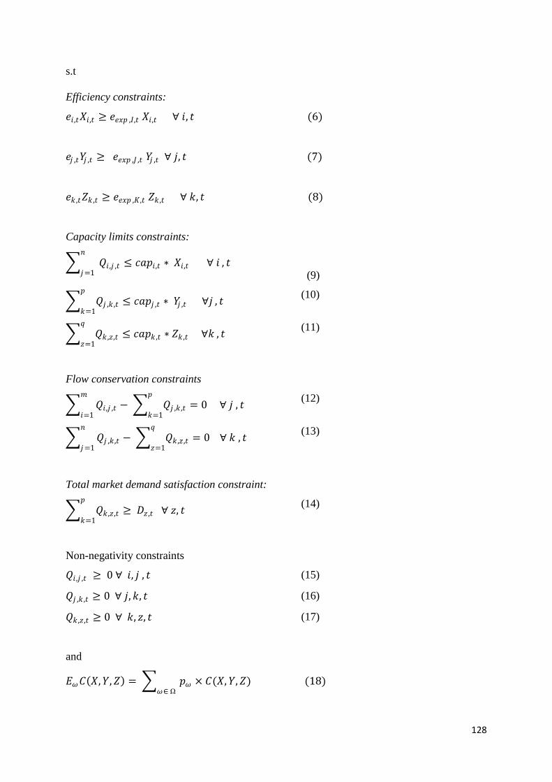
128

s.t


𝑒𝑖 ,𝑡𝑋𝑖,𝑡 ≥ 𝑒𝑒𝑥𝑝 ,𝐼,𝑡 𝑋𝑖,𝑡 ∀ 𝑖, 𝑡 (6)

𝑒𝑗 ,𝑡𝑌𝑗 ,𝑡 ≥ 𝑒𝑒𝑥𝑝 ,𝐽 ,𝑡 𝑌𝑗 ,𝑡 ∀ 𝑗, 𝑡 (7)

𝑒𝑘 ,𝑡𝑍𝑘 ,𝑡 ≥ 𝑒𝑒𝑥𝑝 ,𝐾,𝑡 𝑍𝑘 ,𝑡 ∀ 𝑘, 𝑡 (8)


𝑄𝑖 ,𝑗 ,𝑡 ≤ 𝑐𝑎𝑝𝑖,𝑡 ∗ 𝑋𝑖,𝑡 ∀ 𝑖𝑛

𝑗=1, 𝑡

(9)

𝑄𝑗 ,𝑘 ,𝑡 ≤ 𝑐𝑎𝑝𝑗 ,𝑡 ∗ 𝑌𝑗 ,𝑡 ∀𝑗𝑝

𝑘=1, 𝑡

(10)

𝑄𝑘 ,𝑧,𝑡 ≤ 𝑐𝑎𝑝𝑘 ,𝑡 ∗ 𝑍𝑘 ,𝑡 ∀𝑘𝑞

𝑧=1, 𝑡

(11)


𝑄𝑖 ,𝑗 ,𝑡 − 𝑄𝑗 ,𝑘 ,𝑡 = 0 ∀ 𝑗 , 𝑡 𝑝

𝑘=1

𝑚

𝑖=1

(12)


𝑞

𝑧=1= 0 ∀ 𝑘 , 𝑡

𝑛

𝑗=1

(13)



𝑘=1

(14)


𝑄𝑖 ,𝑗 ,𝑡 ≥ 0 ∀ 𝑖, 𝑗 , 𝑡 (15)

𝑄𝑗 ,𝑘 ,𝑡 ≥ 0 ∀ 𝑗, 𝑘, 𝑡 (16)

𝑄𝑘 ,𝑧 ,𝑡 ≥ 0 ∀ 𝑘, 𝑧, 𝑡 (17)

and

𝐸𝜔𝐶 𝑋, 𝑌, 𝑍 = 𝑝𝜔 × 𝐶(𝑋, 𝑌, 𝑍)𝜔∈ Ω

(18)

129

Constraint sets (2) – (4) restrict every facility to be either open or closed. Constraints (6) –

(8) prohibit the selection of ineffective actors. These efficiency constraints are the same used

in the mathematical model proposed in chapter 2. Efficiency scores are calculated based on

the AHP-OWA procedure. (for more details, see the chapter 2, section 4).

In the above formulation, the objective function minimizes the supply chain total cost,

which includes fixed and variable costs. The variable costs consist of the purchasing costs, the

production costs, and the distribution costs. While the fixed costs consist of the facilities

opening costs, operating costs, and closing costs. The opening costs occur at the period t+1

only if the corresponding facility was closed on the previous period t. Simultaneously, for the

closing costs, they occur at a period t only if the corresponding facility was opened at the

period t-1. These two costs are related to the dynamic nature of the problem.

Constraint sets (9)-(11) stipulate that all shipments from a supplier, a plant, or a

distribution center, must not exceed its maximum capacity. Constraint sets (12)-(13) indicate

a conservation of flow at each facility, while (14) requires that all the market demand must be

met. A non-negativity on each shipment is imposed by constraint sets (15)-(17). The multi-

period nature of the problem is related to the objective function formulation, which involves

the closing and reopening costs. The formulation of these costs includes nonlinear

components. The model is then linearized and based on the available the literature in this

field, (See the previous chapters for more details, and Fortet (1959) ).

5.7 Experimental results

This section presents a small-scale ( 6 suppliers, 3 producers and 3 distributors) supply

chain design problem adapted from a real-life situation.

130

According to the research department of the whole company, four different product life

cycle scenarios are possible.

Scenario 1: (the classical product life cycle) introduction - Growth - Maturity – Decline

Scenario 2: Introduction – growth –Maturity

Scenario 3: Introduction - Decline

Scenario 4 : Introduction – Growth

The respective occurrence probabilities of these scenarios, are : p1=0.6; p2=0.15; p3=0.1;

p4=0.15

Important data used in implementations are presented in Table 5.1.

Table 5.1: Data used in implementations

Denoting by a classical solution, the solution which considers only the classical product

life cycle scenario, we refer to the following percentages for verifying the relevance of our

results:

ΔωSt

: the difference in % between the supply chain total cost given by the optimal solution of

each scenario ω in Ω and the supply chain total cost given by the stochastic solution for the

same scenario.

Description Value

Unit material costs [47, 68]

Unit distribution costs [5,40]

Unit production cost [260, 340]

Fixed cost to operate Suppliers [3.000, 5.000]

Fixed cost to operate Plants [21.000, 35.000]

Fixed cost to operate Distributors [42.000 , 60.000]

Fixed cost to open or close Suppliers [3.000, 150.000]

Fixed cost to open or close Plants [8.000, 180.000]

Fixed cost to open or close Distributors [4.000 , 160.000]

Cumulative sales [0, 90.000]

131

ΔωCl

: the difference in % between the supply chain total cost given by the optimal solution of

each scenario ω in Ω and the supply chain total cost given by the classical solution for the

same scenario.

ΔESt

: the difference in % between the expected supply chain total cost given by the optimal

solution of each scenario ω in Ω and the expected supply chain total cost given by the

stochastic solution for the same scenario.

ΔECl

the difference in % between the expected supply chain total cost given by the optimal

solution of each scenario ω in Ω and the expected supply chain total cost given by the

classical solution (if we consider the classical product life cycle) for the same scenario.

A comparison of the different results; supply chain optimal total cost, the stochastic minimal

total cost, and the classical minimal total cost; for each scenario is presented in table 5.2.

The following table shows the different results obtained for Δω

St

, ΔωCl

, ΔE

St

, and ΔECl

for

the supply chain design problem considered.

Table 5.2: Table of results

Scenarios Stochastic cost Optimal cost Classical cost Δω

St

ΔωCl

1 65668400 65589500 65589500 0.1201 0

2 84553500 82187800 84106300 2.7979 2.2810

3 9968300 9665680 10963100 3.0358 11.8344

4 79126800 79050200 84300800 0.0968 6.2284

Expected 64949915 64505968 65758415 ΔE

St

= 0.6835 ΔECl

= 1.9046

From the table 5.2, we remark that the expected minimal total cost generated by the

stochastic solution is 0.6835% from the expected optimal total cost while the expected

132

minimal total cost generated by the classical solution is 1.9046% from this same expected

optimal total cost value.

5.8 Sensitivity analysis

5.8.1 Sensitivity analysis by changing the scenarios' probabilities

To better analyze these results, we proposed to vary the probabilities of occurrence of the

different scenarios and see the behavior of the two methods with respect to different scenarios

that can happen.

Table 5.3: Table of results for the scenarios' probabilities: (0.05, 0.85, 0.05, 0.05)

scenarios Stochastic cost Optimal cost Classical cost Δω

St

ΔωCl

1 65935400 65589500 65589500 0.5246 0

2 83295300 82187800 84106300 1.3296 2.2810

3 10583000 9665680 10963100 8.6679 11.8344

4 83406800 79050200 84300800 5.2233 6.2284

Expected 78797265 64505968 65758415 1.5513 1.9046



St

ΔωCl

1 65828000 65589500 65589500 0.3623 0

2 82844400 82187800 84106300 0.7926 2.2810

3 10246600 9665680 10963100 5.6694 11.8344

4 82362800 79050200 84300800 4.022 6.2284

Expected 30276140 29448726 31073830 2.7329 5.2298

133



St

ΔωCl

1 65791400 65589500 65589500 0.3069 0

2 84337100 82187800 84106300 2.5485 2.2810

3 10456200 9665680 10963100 7.5603 11.8344

4 79935400 79050200 84300800 1.1074 6.2284

Expected 72720450 71752473 76012015 1.3311 5.6038

Results’ interpretation

From the results ,given by the previous tables, we can conclude that in most cases, the

stochastic method gives better results than the classical one.

Moreover, if we look more closely at the results given by the two different methods for the

scenario with the highest probability of occurrence, except the classical scenario, we can

remark that in all presented cases, the best results were given by the stochastic method.

In table 5.3 for example, scenario 2 has the highest probability of occurrence. If in reality,

scenario 2 happens, the stochastic method will present a cost deviation of 1.3296 % from the

optimal cost, while the classical solution cost deviation will be of 2.2810 %.

Likewise, in table 5.4, for scenario 3, then the stochastic method will present a cost deviation

of 5.66794 % from the optimal cost, while the classical solution cost deviation will be of

11.8344 %.

In table 5.5, the probability of occurrence of scenario 4 was the highest. If in reality, this

scenario will happen, the cost proposed by the stochastic method will be 1.1074% greater than

the optimal cost, while the classical cost will be greater by 6.2284% .

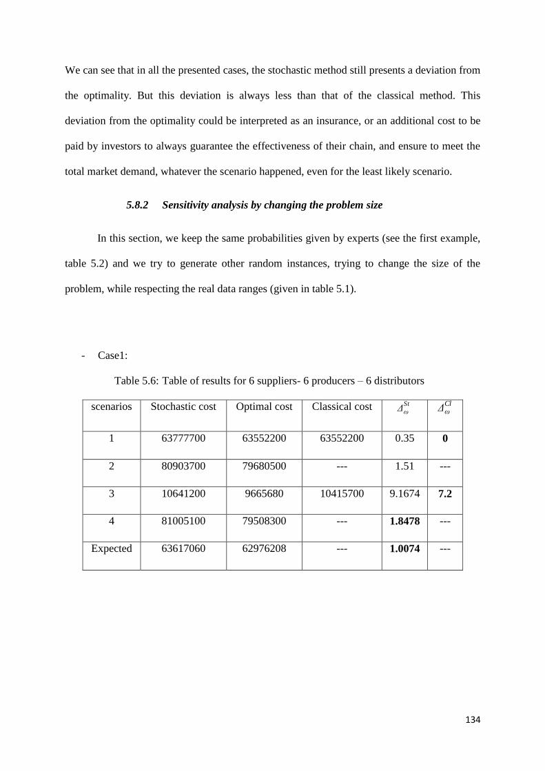
134

We can see that in all the presented cases, the stochastic method still presents a deviation from

the optimality. But this deviation is always less than that of the classical method. This

deviation from the optimality could be interpreted as an insurance, or an additional cost to be

paid by investors to always guarantee the effectiveness of their chain, and ensure to meet the

total market demand, whatever the scenario happened, even for the least likely scenario.

5.8.2 Sensitivity analysis by changing the problem size

In this section, we keep the same probabilities given by experts (see the first example,

table 5.2) and we try to generate other random instances, trying to change the size of the

problem, while respecting the real data ranges (given in table 5.1).

- Case1:

Table 5.6: Table of results for 6 suppliers- 6 producers – 6 distributors


St

ΔωCl

1 63777700 63552200 63552200 0.35 0

2 80903700 79680500 --- 1.51 ---

3 10641200 9665680 10415700 9.1674 7.2

4 81005100 79508300 --- 1.8478 ---

Expected 63617060 62976208 --- 1.0074 ---

135

- Case 2:



St

ΔωCl

1 30500200 30335400 30335400 0.5403 0

2 29997700 29665100 30763300 1.1088 3.5698

3 8388660 7989200 8436600 4.7619 5.3031

4 28692800 28413500 28783100 0.9734 1.2841

Expected 27942561 27711950 27976860 0.8253 0.9469

- Case 3:



St

ΔωCl

1 17075200 16761800 16761800 1.8354 0

2 10403300 9945700 10174700 4.3986 2.2507

3 6435500 6225100 6785400 3.2694 8.2574

4 13080100 12224400 14669200 6.5420 16.6662

Expected 14411180 14005105 14462205 2.8178 3.1607

136

- Case 4:



St

ΔωCl

1 27838700 27556600 27556600 1.0133 0

2 20628300 19955200 20596200 3.2630 3.1122

3 11002000 10991100 12597100 0.0991 12.7490

4 27020700 26788300 26992300 0.8601 0.7558

Expected 24950770 24644595 24931945 1.2271 1.1525

- Case 5:



St

ΔωCl

1 33462300 33255500 33255500 0.6180 0

2 30124700 29988700 30058800 0.4515 0.0023

3 12197500 10988500 13515800 9.9119 18.6989

4 34697200 34627700 34686700 0.2003 0.1701

Expected 31020415 30744610 31016705 0.8891 0.8773

137

- Case 6:



St

ΔωCl

1 29029100 28899100 28899100 0.4478 0

2 27654600 27577600 27613100 0.2784 0.1286

3 22187700 19988100 22786700 9.9136 12.2817

4 28964300 28734500 29223300 0.7934 1.6726

Expected 28129065 27785085 28143590 1.2229 1.2738

Results' interpretation

By analyzing the overall presented results, we can notice that in most cases, the best average

result is given by the stochastic method. However, for the few cases that present the opposite

result, we notice that the difference between costs given by the two methods is really too low.

This is the case for results given by tables 5.9 and 5.10.

Indeed, in table 5.9, the classical method cost presents a deviation of 1.1525% from the

optimality, whereas the classical method cost presents a deviation of 1.2271%.

The same thing for table 5.10, where the classical method cost presents a deviation of

0.8773% from the optimality while, the classical method cost presents a deviation of

0.8891%.

138

- Analyzing the results based on the worst cases.

We note that in the worst situation, if the stochastic solution result is not the best result, it is

however very close to that of the classical solution. In tables 5.7, 5.8, 5.10 and 5.11, the worst

stochastic solution results deviations from the optimal results are respectively of 4.7619%

versus 5.3031% for the classical method, 6.542% versus 16.6662% for the classical method ,

9.9119% versus 18.6989% for the classical method, and 9.9136% versus 12.2817% for the

classical method.

In table 5.9, the worst stochastic solution results deviation from the optimal results is of

3.263% versus 3.1122% for the classical method. We observe that the difference between the

two results is very low and could be negligible.

In table 5.6, the worst stochastic solution results deviations from the optimal results is of

9.16%, while, in the worst case the classical method could not give results for the appropriate

scenario.

Some of the most important weaknesses of the classical method are:

- Unresponsiveness: as the case presented in the table 5.6.

Indeed, in this case, we can see that the solution ,given by the classical method, is unable to

meet several scenarios that can happen, (scenarios 2 and 4 in this instance).

This could result in multiple damages to investors, who could be in a very difficult position,

especially for the out of stock case. In this case, the market demand cannot be met, and this

could incur costs of delays or unmet orders. Though, these high additional costs could be

avoided when using the stochastic method.

139

- Failure to meet the efficiencies

Indeed, when considering the classical scenario only, and that we are in reality faced with a

different scenario, the efficiencies of the preselected actors may not achieve the efficiency

level, fixed by the decision makers. This of course reduces, either slightly or significantly, the

supply chain global efficiency.

5.9 Conclusion

In this chapter, we investigated the problem of designing a supply chain under uncertainty on

the product life cycle. We used a stochastic programming approach to solve this problem.

Based on the comparison between the two methods, we generally conclude that the solutions

obtained by the stochastic programming approach are better than those obtained by the

deterministic one where only the classical product life cycle scenario is considered. The

results obtained point out the effectiveness of the product life cycle uncertainty consideration

in the supply chain design.

140

Effective supply chain design calls for robust analytical models and design tools. Previous

works in this area were mostly Operation Research oriented without considering

manufacturing aspects. Recently, researchers have begun to realize that the decision and

integration effort in supply chain design should be driven by the manufactured product,

specifically, product characteristics and product life cycle. In addition, decision-making

processes should be guided by a comprehensive set of performance metrics.

According to these metrics, a supply chain actors‘ assessment process becomes important and

routine, especially for those companies that manufacture products with short life cycles.

Moreover, these performance metrics are very different and closely dependent on the product

life cycle stages.

Indeed, effective supply chain design and management are envisioned as a solution to meet

the constantly changing needs of the customer at a low cost, high quality, short lead times,

and a high variety.

In this thesis, we proposed models for a multi-period supply chain network design,

highlighting the importance of considering the product life cycle in this strategic supply chain

level.

CHAPTER 6

Conclusion

141

In chapter 3 of this thesis, a two-phase mathematical programming approach was proposed for

effective supply chain network design. In phase I of the decision making process, multi-

criteria efficiency models are utilized to evaluate the performance of suppliers, manufacturers

and distributors depending on the product life cycle stage. In phase II, a mixed integer

programming problem is utilized to design the multi-period supply chain network and to solve

the transshipment problem in order to identify optimal allocation decisions subject to the

actors‘ efficiencies, capacities, and the market demand satisfaction constraints.

An example is used to demonstrate a company‘s establishment of a comprehensive and

objective mechanism of assessment, to screen out potential actors by considering product

strategies at different phases of the product life cycle.

A potential extension to the methodology includes the case of multiple suppliers furnishing

different sets of parts/components. The case of production and delivery of multiple products

across multiple time periods is another interesting issue that needs to be considered.

Chapter 4 presented an extension of the second step of the methodology proposed in chapter

3. We proposed a multi-objective sustainable supply chain network design problem.

We formulated the problem as a Weighted Goal Programming model which aims at achieving

three goals, the economic, environmental and social goals, which are respectively: (i) total

costs goal, (ii) CO2 emissions goal, and (iii) total number of jobs created goal. We conducted

a sensitivity analysis for the case study and we observed that, improving the building

technology, which directly affects the energy requirement for each site, can decrease CO2

emission of the whole network. Also, the total cost increase is expected to be in conflict with

the other two goals that aim at reducing the CO2 emission, and to maximize the total number

of jobs created in the whole supply chain. Regarding the influence of some parameters on the

142

supply chain configuration, we found that a small variability of goals' weight does not affect

the supply chain structure, but only affects significantly the supply chain network. This may

be due to the efficiency constraints, which have a great impact on the supply chain actors‘

selection in the proposed model . Indeed, these constraints remain unchanged against the

variation of the goals' weights.

The research presented in this chapter could be extended through designing new solution

methods to solve this multi-objective supply chain network design model, such as heuristics

and metaheuristics.

Chapter 5 presented a supply chain design problem which includes explicitly uncertainty on

the product life cycle. We used two-stage stochastic programming formulation to model the

problem.

The results obtained pointed out that supply chain design methods which do not include

uncertainty obtain inferior results if compared to models that formalize it implicitly.

The stochastic model, for some possible scenarios, could handle data uncertainty with a

reasonable increase in total costs compared to the deterministic model. However, it can

respond to any possible scenario that can arise. Therefore it can be concluded that the

proposed two-stage programming model can be used as a robust model in real cases.

Many possible future research directions can be defined in the area of supply chain network

design under uncertainty. For example addressing uncertainty for all variable costs at each

product life cycle stage, and potential locations of supply chain actors may be attractive

directions for future research. Moreover, time complexity, when the size of the problem and

the number of scenarios increase, are not addressed in this chapter.

Mathematical models and the two-phase method proposed in this thesis could serve as a basis

for dealing with product-driven supply chain network design problems.

143

Bibliography

[1] Abdallah.T. , Farhat.A. , Diabat. A., and Kennedy.S.,( 2012). Green supply

chains with carbon trading and environmental sourcing: Formulation and life

cycle assessment, Applied Mathematical Modelling 36:4271–4285

[2] Aghezzaf, E. (2005). Capacity planning and warehouse location in supply chains

with uncertain demands. Journal of the Operational Research Society, 56, 453-

462.

[3] Aitken. J, Childerhouse. P, and Towill. D. R.(2003). The impact of product life

cycle on supply chain strategy. International Journal of Production Economics,

85: 127–140.

[4] Akinc U. (1993). Selecting a set of vendors in a manufacturing environment‘,

Journal of Operations Management, 11: 107-122.

[5] Alcada-Almeida, L., Tralhao, L., Santos, L., & Countinho-Rodrigues, J. (2009).

A Multiobjective Approach to Locate Emergency Shelters and Identify

Evacuation Routes in Urban Areas. Geographical Analysis, 41(1): 9-27.

[6] Amini, M. and H. Li. (2011), Supply Chain Configuration for Dynamic Diffusion

of New Products: An Integrated Optimization Approach, Omega , 39( 3): 313-

322.

[7] Arntzen, B. C., Gerald G. B, Terry P. H, and Trafton L. L. (1995). Global Supply

Chain Management at Digital Equipment Corporation, 25: 69-93.

[8] Azaron. A., Borwn, K.N., Tarim, S.A., and Modarres, M. (2008). A multi-

objective stochastic programming approach for supply chain design considering

risk. International Journal of Production Economics, 116: 129-138.

144

[9] Azzone, G. and Noci, G. (1996). Measuring the environmental performance of

new products: an integrated approach‖, International Journal of Production

Research, 34(11): 3055-78.

[10] Barbosa-Povoa, A.P. (2009). Sustainable supply chains . Computer Aided

Chemical Engineering. 27, 127-132.

[11] Barros, A.I., Dekker, R., Scholten, V., (1998). A two-level network for recycling sand:

A case study. European Journal of Operational Research. 110: 199-214.

[12] Beamon, B.M. (1998). Supply chain design and analysis: models and methods.

International Journal of Production Economics. British Journal of Management,7:

63-80

[13] Bellman, R.E., Zadeh, L. (1970) . Decision making in a fuzzy environment.

Management Science. 17 : 141-164.

[14] Benyoucef, L., Xie.X., (2011). Supply Chain Design Using Simulation-Based

NSGA-II Approach. Multi-objective Evolutionary Optimisation for Product

Design and Manufacturing : 455-491.

[15] Besbes, K., Allaoui, H., Goncalves, G., Loukil, T., (2012). A multi-phase

approach for supply chain design with product life cycle considerations. ICNSC

2012: 197-202.

[16] Besbes, K., Allaoui, H., Goncalves, G., Loukil, T., (2013). A supply chain

design with product life cycle and green procurement considerations. ICNSC

2013: 855-860.

[17] Besbes, K., Allaoui, H., Goncalves, G., Loukil, T., A Green supply chain

design with product life cycle considerations. To appear in a special issue of the

Supply Chain Forum : an International Journal.

http://www.informatik.uni-trier.de/~ley/pers/hd/x/Xie:Xiaolan.html

http://www.informatik.uni-trier.de/~ley/db/books/daglib/0027803.html#BenyoucefX11

http://www.informatik.uni-trier.de/~ley/db/books/daglib/0027803.html#BenyoucefX11

http://www.informatik.uni-trier.de/~ley/pers/hd/a/Allaoui:Hamid.html

http://www.informatik.uni-trier.de/~ley/pers/hd/g/Goncalves:Gilles.html

http://www.informatik.uni-trier.de/~ley/pers/hd/l/Loukil:Taicir.html

http://www.informatik.uni-trier.de/~ley/db/conf/icnsc/icnsc2012.html#BesbesAGL12











145

[18] Bidhandi. H. M., and Yusuff. R. M (2011). Integrated supply chain planning

under uncertainty using an improved stochastic approach. Applied Mathematical

Modelling 35: 2618–2630.

[19] Birge, J. R., and Louveaux. F (1997). Introduction to Stochastic Programming.

Springer, New York.

[20] Birou, L.M., Faucet, S.E. and Magnan, G.M. (1998). The product life cycle: a

tool for functional strategic alignment. International Journal of Purchasing and

Materials Management, 34 (2): 37-51.

[21] Bojarski, A. D., Lainez, J. M., Espuna, A., and Puigjaner, L. (2009)

Incorporating environmental impacts and regulations in a holistic supply chains

modeling: An LCA approach. Computers & Chemical Engineering, 33(10):

1747–1759.

[22] Bordogna G., Fedrizzi, M. and Passi G. (1997). A linguistic modeling of

consensus in group decision making based on OWA operators, IEEE

Transactions on Systems, Man, and Cybernetics, 27 (1): 126- 132.

[23] Busby, J.S., Fan, I.S., (1993). The extended manufacturing enterprise: Its

nature and its needs. International Journal of Technology Management 8 (4):

294–308.

[24] Butner, K., Geuder, D., Hittner, J., (2008). Mastering carbon management:

balancing trade-offs to optimize supply chain efficiencies. IBM Global Business

Services, Somers, NY.

[25] Buzzell, R, and Nourse, R. (1967). Product innovation in food processing:

Division of Research, Graduate School of Business Administration, Harvard

University, Boston, pp: 1954-1964.

146

[26] Buzzell. R. (1966). Competitive behavior and product life cycles,

in New Ideas for Successful Marketing, John Wright and Jac Goldstucker, eds.,

Chicago: American Marketing Association.

[27] Byrne, A.J., (1993) The virtual corporation. Business Week 3304 (February),

98–103

[28] Canel, C., Khumawala, B.M. (1997). Multi-period international facilities

location: An algorithm and application, International Journal of Production

Economics, 35: 1891-1910.

[29] Canel, C., Khumawala, B.M., Law, J., Loh, A. (2001). An algorithm for the

capacitated, multi-commodity multi-period facility location problem, Computers

& Operations Research, 28: 411-427.

[30] Carr, A.S., Smeltzer, L.R. (1999a). The relationship of strategic purchasing to

supply chain management. European Journal of Purchasing & Supply

Management, 5: 43-51.

[31] Carr, A.S., Smeltzer, L.R. (1999b). The relationship among purchasing,

benchmarking, strategic purchasing, firm performance, and firm size. Journal of

Supply Chain Management, 35(4): 51-60.

[32] Cavinato, J., (1987). Product life cycle: logistics rides the roller coaster.

Journal of Distribution, September,pp: 12–20.

[33] Chaabane, A., Ramudhin, A., and Paquet, M. (2012). Design of sustainable

supply chains under the emission trading scheme. International Journal of

Production Economics, 135(1): 37-49.

[34] Chang. S. L, Wang. R. C, and Wang. S. Y.(2006). Applying fuzzy linguistic

quantifier to select supply chain partners at different phases if product life cycle.

International Journal of Production Economics, 100: 348-359.

147

[35] Charnes, A., Cooper, W.W. (1961). Management Models and Industrial

Applications of linear Programming, Wiley, New York.

[36] Charnes, A., Cooper, W.W., Ferguson, R. (1955). Optimal estimation of

executive compensation by linear programming Management Science. 1: 138-

151.

[37] Chen, C. L, Lee, W.C. (2004) . Multi-objective optimization of multi-echelon

supply chain networks with uncertain product demands and prices, Computers

and Chemical Engineering, 28: 1131-1144.

[38] Chen. P. Y. (2012). The investment strategies for a dynamic supply chain

under stochastic demands. International journal of production economics 139 :

80–89.

[39] Christopher, M. and Towill, D.R. (2002). Developing Market Specific Supply

Chain Strategies‖, International Journal of Logistics Management,13 ( 1): 1-14.

[40] Cox, A. and Lamming. R. (1997). Managing Supply in the firm of the future.

European Journal of Purchasing and Supply Management 3(2): 53-62.

[41] Cox. W. (1967). Product life cycles as marketing models, Journal of Business ,

40: 375-384.

[42] Cunningham, M,T. (1969). The application of product life cycles to corporate

strategy: some research findings. European Journal of Marketing, 3 : 32-44.

[43] Dean. J.(1950). Pricing policies for new products. Havard business review, 28:

45-53, 1950.

[44] Dehghanian, F., Mansour, S. (2009). Designing sustainable recovery network

of end-of-life products using genetic algorithm, Resources, Conservation and

Recycling, 53, 559-570.

http://www.ingentaconnect.com/content/mcb/007

148

[45] Dogan, K., Goetschalckx, M. (1999). A primal decomposition method for the

integrated design of multi-period production–distribution systems, IIE

Transactions, 31, 1027-1036.

[46] Dolgui, A., and Proth, J. M., (2010). Supply Chain Engineering: Useful

Methods and Techniques. Springer, ISBN: 978-1-84996-016-8.

[47] Dolgui, A., Soldek, J., and Zaikin, O., (2005). Supply chain optimization:

product/process design, facilities location and flow control, Series: Applied

Optimization, 94, Springer.

[48] Dubois, D., and Prade, H., (1985). A review of fuzzy sets aggregation

connectives. Information Science 36: 85- 121.

[49] Dupacova, J. (1996). Scenario-based stochastic programs: Resistance with

respect to sample.Annals of Operations Research. 64, 21-38.

[50] Dyer, M., & Stougie, L. (2006). Computational complexity of stochastic

programming problems. Mathematical Programming, 106, 423-432.

[51] Elhedhli. S. and Merrick.R. (2012). Green supply chain network design to

reduce carbon emissions. Transportation Research Part D: Transport and

Environment, 17(5):370 – 379.

[52] Ferguson E.L., Darmon N., Fahmida U., Fitriyanti S., Harper T.B.,

Premachandra I.M., (2006). Design of Optimal Food-Based Complementary

Feeding Recommendations and Identification of Key ‗Problem Nutrients‘ Using

Goal Programming. The Journal of Nutrition. 136: 2399-2404

[53] Fisher, M.L., (1997). What is the right supply chain for your product? Harvard

Business Review 75:105–116.

[54] Fortet, R. (1959). L‘algèbre de boole et ses applications en recherche

opérationnelle. Cahier du centre d‘étude de Recherche Opérationnelle. 4 : 5-36.

http://www.emse.fr/en/transfert/g2i/personnel/dolgui_a/New_book_by_Dolgui_and_Proth.pdf



http://www.springer.com/engineering/production+eng/book/978-1-84996-016-8

http://www.springer.com/math/applications/book/978-0-387-23566-0

http://www.springer.com/math/applications/book/978-0-387-23566-0

149

[55] Fortet, R. (1960). Applications de 1'Algèbre de Boole en Recherche

Opérationnelle. Revue Française d‘informatique et de Recherche Opérationelle

4:17–26.

[56] Frederixon, M. (1969). An investigation of the product life cycle concept and

its application to new product proposal evaluation within the chamical industry.

PhD dissertation, Michigan state university.

[57] Gadde, L-E. and Håkansson, H. (2001), Supply Network Strategies. John

Wiley &Sons, Chichester.

[58] Gattorna, J. and Walters, D. (1996), Managing the Supply Chain. Anthon

Rowe Ltd.

[59] Ghodsypour, S. H., & O‘Brien, C. (1998). A decision support system for

supplier selection using an integrated analytic hierarchy process and linear

programming. International Journal of Production Economics, 56–57, 199–212.

[60] Goh, M., Lim, J.I.S., Meng, F. (2007). A stochastic model for risk management

in global supply chain networks. European Journal of Operational Research, 182,

164-173

[61] Goldman, L.S., (1994). Co-operating to compete. CMA Magazine 68 (2): 13–

17

[62] Guan, Z. , Philpott, A.B. (2011). A multistage stochastic programming model

for the New Zealand dairy industry, International Journal of Production, 134,

289-29.

[63] Guillen, G., Grossmann, I.E. (2009). Optimal design and planning of

sustainable chemical supply chains under uncertainty . AIChE Journal, 55(1), 99-

121.

150

[64] Harland, C. (1996). Supply Chain Management: Relationships, Chains and

Networks.

[65] Hayes, R.H., Wheelwright, S.C., (1979). Link Manufacturing Process and

Product Life Cycles. Harvazrd Business Review,March–April, 127–136.

[66] Headen, R. (1966). The introductory Phases of the product life cycle for new

grocery products: consumer acceptance and competitive behavior. Phd

dissertation, Havard university, Cambridge.

[67] Herrera, F., Herrera-Viedma, E., Martinez, L.(2000). A fusion approach for

managing multi-granularity linguistic term sets in decision making. Fuzzy Sets

and Systems .114 (1): 43–58.

[68] Hill, T. (1985), Manufacturing Strategy, Macmillan Education, London

[69] Hines,T. (2004), Supply Chain Strategies: Customer Driven and Customer

Focused, Oxford: Elsevier ISBN 0750655518 408 pages.

[70] Hinkle. J, .(1966). Life cycle. Nielsen, New York.

[71] Hinojosa, Y., Kalcsics, J., Nickel, S., Puerto, J., Velten, S. (2008). Dynamic

supply chain design with inventory, Computers & Operations Research, 35: 373-

391.

[72] Hinojosa, Y., Puerto, J., Fernández, F.R. (2000). A multiperiod two-echelon

multicommodity capacitated plant location problem, European Journal of

Operational Research, 123:271-291.

[73] Holland, C. P. (1995). Cooperative supply chain management: the impact of

interorganizational information systems Journal of Strategic Information

Systems 4( 2): 117-133.

151

[74] Huang, S.H., Uppal, M., Shi, J., (2002). A product driven approach to

manufacturing supply chain delection. Supply Chain Management: An

International Journal 7 (3/4): 189–199

[75] Iacocca Institute, (1991). 21st Century Manufacturing Strategy. Lehigh

University, Bethlehem, PA.

[76] Jaegler, A., and Burlat, P., (2012). Carbon friendly supply chains: a simulation

study of different scenarios. Production Planning & Control 23 (4), 269-278.

[77] Johnston, R., Lawrence, L.R., (1988). Beyond vertical integration – the rise of

the value-adding partnership. Harvard Business Review 66 (4): 94–101.

[78] Jones, D.F. and Tamiz, M .(2010). Practical Goal Programming. Springer, New

York.

[79] Kacprzyk, J. (1986). Group Decision Making with a Fuzzy Linguistic Majority.

Fuzzy Sets and Systems 18: 105-118.

[80] Kall, P., and Mayer, J., (2005). Stochastic Linear Programming. Springer, New

York.

[81] Kall, P., and Wallace, S. W., (1994). Stochastic programming. New York, NY:

Wiley.

[82] Khurrum. S.B, and Huq .F, (2002). Supplier selection problem: A comparison

of the total cost of ownership and analytical hierarchy process approaches.

Supply Chain Management , An International journal, 7(3): 126-135

[83] Klibi, W., Martel, A., and Guitoni, A. (2010). The design of robust value-

creating supply chain networks: a critical review. European Journal of

Operational Research, 203( 2): 283-293.

[84] Kotler. P (1994) Marketing Management, 8th edition, Prentice Hall, New York

http://scholar.google.fr/citations?view_op=view_citation&hl=fr&user=wU171gcAAAAJ&citation_for_view=wU171gcAAAAJ:Zph67rFs4hoC



152

[85] Krause, D.R., Scannell, T.V., and Calantone, R.J. (2000). A structural analysis

of the effectiveness of buying firm‘s strategies to improve supplier performance.

Decision Sciences, 31 (1): 33–55

[86] Ku, C. Y., Chang, C. T.,and Ho, H. P. (2010). Global supplier selection using

fuzzy analytic hierarchy process and fuzzy goal programming. Quality and

Quantity, 44(4): 623-640.

[87] Kumar, M., Thurow, K., Stoll, N. and Stoll, R. (2008). A fuzzy system for

modeling the structure-activity relationships in presence of uncertainties,

Proceedings of the IEEE International Conference on Automation Science and

Engineering (CASE 2008), Washington DC, USA, pp. 1025– 1030.

[88] Lahdelma, R., Salminen, P., Hokkanen, J. (2002). Locating a waste treatment

facility by using stochastic multicriteria acceptability analysis with ordinal

criteria, European Journal of Operational Research, 142, 345-356.

[89] Lajili,I., Ladhari, T., and Babai, M. Z., (2013). Multi-Criteria Inventory

Classification Problem: A consensus approach. Published in the 5th International

Conference on Modeling, Simulation and Applied Optimization (ICMSAO), 28-

30 April 2013, Hammamet, Tunisia.

[90] Lambert, A., (2009). Résolution de programmes quadratiques en nombres

entiers. PhD thesis in computer science, CEDRIC.

[91] Lee, L. W., Wang, L. H., Chen, S. M., & Leu, Y. H. (2006b). Handling

forecasting problems based on two-factors high-order fuzzy time series. IEEE

Transactions on Fuzzy Systems, 14(3): 468–477.

[92] Lemathe. P, Balakrishnan. N., (2005). Environmental considerations on the

optimal product mix. European journal of operational research, 167, 398-412.

http://ieeexplore.ieee.org/xpl/mostRecentIssue.jsp?punumber=6547264

http://ieeexplore.ieee.org/xpl/mostRecentIssue.jsp?punumber=6547264

153

[93] Leung , S.C.H., and Wub, Y. (2004). A robust optimization model for

stochastic aggregate production planning, Production Planning and Control, 15:

502-514.

[94] Leung , S.C.H., Tsang, S.O.S., Ng, W.L., and Wu, Y. (2007). A robust

optimization model for multi-site production planning problem in an uncertain

environment. European Journal of Operational Research, 181 : 224-238.

[95] Liang, T.F., Cheng, H.W. (2008). Application of fuzzy sets to manufacturing/

distribution planning decisions with multi-product and multi-time period in

supply chains. Expert Systems with Applications 36 : 3367-3377.

[96] Liberti. L., (2007). Compact linearization for binary quadratic problems. A

quarterly journal of operations research. 5 (3): 231-245.

[97] Listes, O., Dekker, R. (2005). A stochastic approach to a case study for product

recovery network design, European Journal of Operational Research, 160, 268-

287.

[98] Liu, B., (2008). Theory and Practice of Uncertain Programming. 3rd edition.

Beijing, China, Tsinghua University, Department of Mathematical Sciences:202

p.

[99] Liu, X., Sun, J. (2004). A new decomposition technique in solving multistage

stochastic linear programs by infeasible interior point methods, Journal of Global

Optimization, 28, 197-215.

[100] Mak, W.K., Morton, D.P., Wood, R.K. (1999). Monte Carlo bounding

techniques for determining solution quality in stochastic programs, Operations

Research Letters, 24, 47-56.

[101] Malczewski, J. (2006). Ordered weighted averaging with fuzzy quantifiers:

GIS-based multi-criteria evaluation for land-use suitability analysis.

http://www.springerlink.com/content/?Author=Leo+Liberti

http://www.springerlink.com/content/1619-4500/



154

International Journal of Applied Earth Observations and Geoinformation. 8 (4):

270–277.

[102] Martel J.M., Aouni B., (1998) . Diverse Imprecise Goal Programming Model

Formulations. Journal of Global Optimization. 12: 127-138

[103] Mason-Jones, R., Naylor, J.B., and Towill, D., (2000). Engineering the Leagile

Supply Chain. International Journal of Agile Management Systems, 2( 1): 54-61.

[104] Melo, M. T., Nickel, S., and Saldanha-da-Gama, F., (2009). Facility location

and supply chain management—A review. European Journal of Operational

Research, 196(2): 401–412.

[105] Mentzer, J.T., DeWitt, W., Keebler, J.S., Min, S., Nix, N.W., Smith, C.D. and

Zacharia, Z.G., (2001). What is supply chain management. in Mentzer, J.T. (Ed.),

Supply Chain Management, Sage, Thousand Oaks, CA, pp. 1-25.

[106] Miranda, P.A., Garrido, R.A. (2004). Incorporating inventory control decisions

into a strategic distribution network design model with stochastic demand,

Transportation Research Part E: Logistics and Transportation Review, 40, 183-

207.

[107] Nagurney, A., (2009). A system-optimization perspective for supply chain

network integration: the horizontal merger case. Transportation Research. 45: 1-

15.

[108] Narasimhan, R., Das, A., (1999). An empirical investigation of the contribution

of strategic sourcing to manufacturing flexibilities and performance. Decision

Sciences 30: 683–718.

[109] Narasimhan. R, Talluri. S, and Mahapatra. S. K., (2006). Multi-product,

multicriteria model for supplier selection with product life cycle considerations.

Decision Sciences, 37: 577-603.

155

[110] Pagh, J. D., and Cooper, M., (1998). Supply Chain Postponement and

Speculation Strategies: How to choose the right strategy. Journal of Business

Logistics, 19(2): 13-33.

[111] Pan, S., Ballot, E., Fontane, F. (2009). The reduction of greenhouse gas

emissions from freight transport by merging supply chains . International

Conference of Industrial Engineering and Systems Managment, IESM, Montreal,

Canada.

[112] Patton, A., (1959). Stretch your product‘s earning years: top management‘s

stake in the product life cycle. Management review, 38: 9-14, 67-70.

[113] Porter, M. E., (1980). Competitive Strategy. The Free Press, New York.

[114] Price, H. (1996). The anthropology of the supply chain: Fiefs, clans, witch-

doctors and professors. European Journal of Purchasing & Supply Management,

2(2/3): 87 - 105.

[115] Ramudhin, A., Chaabane, A. (2010). Carbon market sensitive sustainable

supply chain network design. International Journal of Management Science and

Engineering Management, 5 (1), 30-38.

[116] Reed, P. (2002). Strategic marketing planning. Nelson, Australia: Thompson

Publishing.

[117] Rehman T., Romero C., (1987). Goal Programming with penalty functions and

livestock ration formulation. Agricultural Systems. 23( 2) : 117-132.

[118] Rink , D. R, and Dodge. R, H., (1980). Industrial sales emphasis across the life

cycle. Industrial marketing management, 9: 305-310.

[119] Rink, D. and Swan, J. (1979). Product life cycle research : A the literature

review. Journal of business Research 7(3): 219–242.

http://orbit.dtu.dk/en/publications/supply-chain-postponement-and-speculation-strategies-how-to-choose-the-right-strategy(6ff33fa7-cabf-4c44-a285-ea41e04e84b6).html



http://orbit.dtu.dk/en/journals/journal-of-business-logistics(f2faa403-1281-4546-ac8b-2628b0f3577b).html



156

[120] Rink, D. R. and Fox, H. W. (1999). Strategic procurement planning across the

product's sales cycle: A conceptualization. Journal of Marketing Theory &

Practice, 7(2): 28-42.

[121] Roghanian, E., Sadjadi. S.J., Aryanezhad. M.B., (2007). A probabilistic bi-

level linear multi-objective programming problem to supply chain planning.

Applied Mathematics and Computation, 188: 786–800.

[122] Romero, C.(2004). A general structure of achievement function for a goal

programming model, European Journal of Operational Research 153 :675–686.

[123] Saaty, T.L, (1990). An Exposition of the AHP in Reply to the Paper :Remarks

on the Analytic Hierarchy Process. Management Science 36(3): 259-268.

[124] Saaty, T.L., (1977). A scaling method for priorities in hierarchical structures.

Journal of mathematical psychology 15(3): 234-281.

[125] Saaty, T.L., (1980). Analytic Hierarchy Process, Planning, Priority Setting,

Resource Allocation. McGraw-Hill, New York.

[126] Santosh K. M. , Ajay. D , and Narasimhan. R. ,(2012). A contingent theory of

supplier management initiatives: Effects of competitive intensity and product life

cycle, Journal of Operations Management 30:406–422.

[127] Santoso, T. , Ahmed, S., Goetschalckx, M., Shapiro, A. (2005). A stochastic

programming approach for supply chain network design under uncertainty,

European Journal of Operational Research, 167, 96-115.

[128] Sarkis, J., (2006). Greening the Supply Chain. Springer, London.

[129] Sen, S., Higle, J.H. (1999). An introductory tutorial on stochastic linear

programming models. Interfaces, 29, 33-61.

[130] Silver, E.A., (1985). Decision systems for inventory management and

production planning. 2nd edition, Wiley, New York.

157

[131] Simchi-Levi, D. and Zhao. Y., (2003). The Value of Information Sharing in a

Two-stage Supply Chain with Production Capacity Constraints. Naval Research

Logistics, 50: 888-916.

[132] Singh, R. K., Benyoucef, L., (2013). A consensus based group decision

making methodology for strategic selection problems of supply chain

coordination. Engineering Applications of Artificial Intelligence 26(1): 122-134.

[133] Smith, A.E, and Coit, W.D., (1995). Penalty Functions. Section C 5.2 of

Handbook of Evolutionary Computation, September.

[134] Snow, C.C, Miles, R.E., Coleman, H.J., (1992). Managing 21st century network

organizations. Organizational Dynamics 20 (3): 5–20.

[135] Srivastava, S. K. (2007). Green supply-chain management: A state-of-the-art

literature review, International Journal of Management Reviews, 9, 1468-2370.

[136] Thomas, D.J. and Griffin. P.M. (1996). Coordinated supply chain

management.

[137] Thomas,A., Genin,P., and Lamouri, S., (2008). Mathematical Programming

Approaches for Stable Tactical and Operational Planning in Supply Chain and

APS Context. Journal of Decision Systems 17(3): 425-455.

[138] Tibben-Lembke, R. S. (2002). Life after death: reverse logistics and the

product life cycle . International Journal of Physical Distribution & Logistics

Management. 32 (3): 223-244.

[139] Turkay, M. C., Oruc, K. F., and Asakura, T., (2004). Multi-company

collaborative supply chain management with economical and environmental

considerations Computers & Chemical Engineering, 28: 985–992.

http://www.informatik.uni-trier.de/~ley/pers/hd/s/Singh:R=_K=.html

http://www.informatik.uni-trier.de/~ley/db/journals/eaai/eaai26.html#SinghB13

http://www.informatik.uni-trier.de/~ley/db/journals/eaai/eaai26.html#SinghB13

http://www.informatik.uni-trier.de/~ley/pers/hd/t/Thomas:Andr=eacute=.html

http://www.informatik.uni-trier.de/~ley/pers/hd/g/Genin:Patrick.html

http://www.informatik.uni-trier.de/~ley/db/journals/jds/jds17.html#ThomasGL08

158

[140] Tuzkaya, U. R., & Önüt, S., (2008). A fuzzy analytic network process based

approach to transportation-mode selection between Turkey and Germany: A case

study. Information Sciences, 178: 3133–3146.

[141] Vonderembse. M.A., Uppal. M, Huang. S.H and Dismukes. J. P., (2006)

Designing supply chains: Towards theory development. International Journal of

Production Economics, 100: 223-238.

[142] Wang G.E, , Huang S.H, Dismukes J.O., (2004). Product-driven supply chain

selection using integrated multi-criteria decision-making

methodology. International Journal of Production Economics, 91: 1-15.

[143] Wang, F., Lai, X., Shi, N. (2011). A multi-objective optimization for green

supply chain network design, Decision Support Systems, 51, 262-269.

[144] Wang, Y., Potter.A, Naim. M., and Beevor. D.,(2011). A case study exploring

drivers and implications of collaborative electronic logistics marketplaces.

Industrial Marketing Management, 40: 612-623.

[145] Wang,S. Y., Chang.S. L., and Wang. R. C., (2009). Assessment of supplier

performance based on product-development strategy by applying multi-

granularity linguistic term sets. Omega, 37: 215 – 226.

[146] Weber, C. A., Current, J. R. and Desai, A., (2000). An optimization approach

to determining the number of vendors to employ. Supply Chain Management:

An International Journal, 2(5): 90‐98.

[147] Weber, C.A., and Ellram, L.M.,(1993). Supplier selection using multiobjective

programming: A decision support systems approach, International Journal of

Physical Distribution and Logistics management, 23 (2): 3-14.

[148] Wiersema, F.D., (1982). Strategic marketing and the product life cycle.

Marketing Science Institute, Cambridge, MA, April.

159

[149] Yager, R. R., (1993). Families of OWA operators. Fuzzy Sets and Systems, 59:

125-148.

[150] Yager, R.R., (1996). Quantifier guided aggregation using OWA operators.

International Journal of Intelligent Systems 11 (1) : 49–73.

[151] Yager. R.R. (1988). On ordered weighted averaging aggregation operators in

multi-criteria decision making. IEEE Transactions on Systems, Man and

Cybernetics 18 (1): 183–190.

[152] Yager. R.R., and Kelman.A., (1999). A. An extension of the analytical

hierarchy process using OWA operators. Journal of Intelligent and Fuzzy

Systems. 7 (4): 401–417.

[153] Yildirim, M. B. and Hearn, D. W., (2005). A First Best Toll Pricing

Framework for Variable Demand Traffic Assignment Problems. Transportation

Research-B, 39: 659-678.

[154] Yu, C.S., Li, H.L. (2000). A robust optimization model for stochastic logistic

problems. International Journal of Production Economics, 64, 385-397.

[155] Zadeh, L.A., (1983). A computational approach to fuzzy quantifiers in natural

languages. Computers and Mathematics with Applications 9 : 149–184.

[156] Zadeh. L. A.,(1975).The concept of a linguistic variable and its application to

approximate reasoning - I," Information Sciences, 8( 3): 199-249.

[157] Zhong, H.Z., (2011). Designing Sustainable Supply Chain Networks.

Unpublished master dissertation. Montreal, Quebec, Canada.

[158] Zhou, Z., Cheng, S., and Hua, B., (2000). Supply chain optimization of

continuous process industries with sustainability considerations. Computers and

Chemical Engineering, 24: 1151–1158.

http://dx.doi.org/10.1016/0020-0255(75)90036-5

http://dx.doi.org/10.1016/0020-0255(75)90036-5

161

Appendix A

More details on how to calculate the suppliers‘ efficiency scores in the introduction stage, for

the example presented in section 3.6 in chapter 3, are given in the following tables.

Table A.1. Pairwise comparison of the sub-criteria relative to the criterion ‗Cost‘ and

relative weights

Fixed cost Normal unit cost Minimum order quantity Weights

Fixed cost 1 5 1/7 0.173

Normal unit cost 1 1/9 0.054

Minimum order quantity 1 0.772

Table A.2. AHP scores for the cost criterion at the introduction stage

S1 S 2 S 3 S 4 S 5 S 6

Fixed cost 0.025 0.075 0.398 0.025 0.398 0.075

Normal unit cost 0.056 0.069 0.349 0.069 0.349 0.105

Minimum order quantity 0.036 0.451 0.232 0.121 0.121 0.036

162

Table A.3. Pairwise comparison of the sub-criteria relative to the criterion ‗Quality‘ and

relative weights

Humidity Rate of oil Grain size Weights

Humidity 1 3 5 0.617

Rate of oil 1 5 0.296

Grain size 1 0.066

Table A.4. AHP scores for the criterion ‗Quality‘ at the introduction stage

S1 S 2 S 3 S 4 S 5 S 6

Humidity 0.101 0.031 0.295 0.428 0.111 0.03

Rate of oil 0.068 0.189 0.409 0.124 0.139 0.068

Grain size 0.2 0.2 0.421 0.066 0.066 0.042

Table A.5. Pairwise comparison of the sub-criteria relative to the criterion ‗service‘ and

relative weights

Packaging Stockout Additional service Weights

Packaging 1 5 1/7 0.085

Stockout 1 1/9 0.617

Additional service 1 0.296

163

Table A.6. AHP scores for the criterion ‗Service‘ at the introduction stage

S1 S 2 S 3 S 4 S 5 S 6

Packaging 0.056 0.18 0.023 0.18 0.502 0.056

Stockout 0.276 0.276 0.071 0.027 0.071 0.276

Additional service 0.394 0.025 0.125 0.072 0.025 0.356

Table A.7. Pairwise comparison of the sub-criteria relative to the criterion ‗Response‘

and relative weights

Normal

delivery LT

Requiring LT to

changing volume

Requiring LT to

changing design

Weights

Normal delivery LT 1 5 9 0.721

Requiring LT to

changing volume 1 7 0.227

Requiring LT to

changing design 1 0.051

Table A.8. AHP scores for the criterion ‗Response‘ at the introduction stage

S1 S 2 S 3 S 4 S 5 S 6

Normal delivery LT 0.044 0.178 0.178 0.025 0.512 0.044

Requiring LT to

changing volume

0.055 0.055 0.277 0.277 0.055 0.277

Requiring LT to changing design 0.227 0.045 0.227 0.227 0.045 0.227

Linguistic Quantifiers for the different criteria in the introduction stage:

R&D: At least half

Cost: Most

Quality: Most

Service: As many as possible

Response: Most

164

Table A.9. OWA weights for the criterion ‗R&D‘ in the introduction stage

S1 S2 S3

Ordered

AHP scores

Corresponding

AHP weights

OWA

weights

Ordered

AHP Scores

Corresponding

AHP weights

OWA

weights

Ordered

AHP Scores

Corresponding

AHP weights

OWA

weights

0.505 0.218 0.436 0.23 0.714 1 0.357 0.066 0.132

0.23 0.714 0.564 0.116 0.218 0 0.116 0.218 0.436

0.071 0.066 0 0.071 0.066 0 0.057 0.714 0.432

S4 S5 S6

Ordered

AHP Scores

Corresponding

AHP weights

OWA

weights

Ordered

AHP Scores

Corresponding

AHP weights

OWA

weights

Ordered

AHP Scores

Corresponding

AHP weights

OWA

weights

0.23 0.714 1 0.357 0.066 0.132 0.22 0.714 1

0.071 0.066 0 0.23 0.714 0.436 0.116 0.218 0

0.029 0.218 0 0.218 0.218 0.432 0.071 0.066 0

165

Table A.10. OWA weights for the criterion ‗Cost‘ in the introduction stage

S1 S2 S3

Ordered

AHP scores

Corresponding

AHP weights

OWA

weights

Ordered

AHP Scores

Corresponding

AHP weights

OWA

weights

Ordered

AHP Scores

Corresponding

AHP weights

OWA

weights

0.056 0.054 0 0.451 0.772 0.944 0.398 0.173 0

0.036 0.772 1 0.075 0.173 0.056 0.349 0.054 0

0.025 0.173 0 0.069 0.054 0 0.232 0.772 1

S4 S5 S6

Ordered

AHP Scores

Corresponding

AHP weights

OWA

weights

Ordered

AHP Scores

Corresponding

AHP weights

OWA

weights

Ordered

AHP Scores

Corresponding

AHP weights

OWA

weights

0.121 0.772 0.944 0.398 0.173 0 0.105 0.054 0

0.069 0.173 0.056 0.349 0.054 0 0.075 0.173 0

0.025 0.054 0 0.121 0.772 1 0.036 0.772 1

166

Table A.11. OWA weights for the criterion ‗Quality‘ in the introduction stage

S1 S2 S3

Ordered

AHP scores

Corresponding

AHP weights

OWA

weights

Ordered

AHP Scores

Corresponding

AHP weights

OWA

weights

Ordered

AHP Scores

Corresponding

AHP weights

OWA

weights

0.2 0.085 0 0.2 0.085 0 0.421 0.085 0

0.101 0.617 0.634 0.189 0.297 0.164 0.409 0.296 0.164

0.068 0.297 0.366 0.031 0.617 0.836 0.295 0.617 0.836

S4 S5 S6

Ordered

AHP Scores

Corresponding

AHP weights

OWA

weights

Ordered

AHP Scores

Corresponding

AHP weights

OWA

weights

Ordered

AHP Scores

Corresponding

AHP weights

OWA

weights

0.428 0.617 0.634 0.139 0.296 0 0.068 0.296 0

0.124 0.296 0.366 0.111 0.617 1 0.042 0.085 0.162

0.066 0.085 0 0.066 0.085 0 0.03 0.617 0.838

167

Table A.12. OWA weights for the criterion ‗Service‘ in the introduction stage

S1 S2 S3

Ordered

AHP scores

Corresponding

AHP weights

OWA

weights

Ordered

AHP Scores

Corresponding

AHP weights

OWA

weights

Ordered

AHP Scores

Corresponding

AHP weights

OWA

weights

0.394 0.296 0 0.276 0.617 0.234 0.125 0.296 0

0.276 0.617 0.824 0.18 0.085 0.17 0.071 0.617 0.824

0.056 0.085 0.176 0.025 0.296 0.596 0.023 0.085 0.176

S4 S5 S6

Ordered

AHP Scores

Corresponding

AHP weights

OWA

weights

Ordered

AHP Scores

Corresponding

AHP weights

OWA

weights

Ordered

AHP Scores

Corresponding

AHP weights

OWA

weights

0.18 0.085 0 0.502 0.085 0 0.356 0.296 0

0.072 0.617 0.404 0.071 0.296 0 0.276 0.617 0.824

0.027 0.296 0.596 0.027 0.617 1 0.056 0.085 0.176

168

Table A.13. OWA weights for the criterion ‗Response‘ in the introduction stage

S1 S2 S3

Ordered

AHP scores

Corresponding

AHP weights

OWA

weights

Ordered

AHP Scores

Corresponding

AHP weights

OWA

weights

Ordered

AHP Scores

Corresponding

AHP weights

OWA

weights

0.227 0.051 0 0.178 0.721 0.842 0.277 0.227 0

0.055 0.227 0 0.055 0.227 0.158 0.227 0.051 0

0.044 0.721 1 0.045 0.051 0 0.178 0.721 1

S4 S5 S6

Ordered

AHP Scores

Corresponding

AHP weights

OWA

weights

Ordered

AHP Scores

Corresponding

AHP weights

OWA

weights

Ordered

AHP Scores

Corresponding

AHP weights

OWA

weights

0.512 0.721 0.842 0.055 0.227 0 0.277 0.227 0

0.277 0.227 0.158 0.045 0.051 0 0.227 0.051 0

0.227 0.051 0 0.044 0.721 1 0.044 0.721 1

169

Table A.14. The AHP-OWA scores for the different criteria at the introduction stage

S1 S 2 S 3 S 4 S 5 S 6

R&D 0.35 0.23 0.51 0.23 0.25 0.22

Cost 0.03 0.43 0.23 0.12 0.12 0.03

Quality 0.09 0.06 0.31 0.32 0.11 0.03

Service 0.24 0.11 0.06 0.04 0.03 0.24

Response 0.04 0.16 0.18 0.47 0.04 0.04

Linguistic Quantifiers for the overall criteria aggregation in the introduction stage: Most

170

Table A.15. The aggregation weights

S1 S2 S3

Ordered

scores

Corresponding

weights

Aggregation

weights

Ordered

Scores

Corresponding

weights

Aggregation

weights

Ordered

Scores

Corresponding

weights

Aggregation

weights

0.35 0.051 0.442 0.43 0.129 0 0.51 0.5128 0.442

0.24 0.033 0.066 0.23 0.512 0.6834 0.31 0.2614 0.5064

0.09 0.261 0.492 0.16 0.063 0.12766 0.23 0.1289 0.0516

0.04 0.063 0 0.11 0.033 0.066 0.18 0.0633 0

0.03 0.128 0 0.06 0.261 0.1234 0.06 0.033 0

S4 S5 S6

Ordered

Scores

Corresponding

weights

Aggregation

weights

Ordered

Scores

Corresponding

weights

Aggregation

weights

Ordered

Scores

Corresponding

weights

Aggregation

weights

0.47 0.0633 0 0.25 0.5128 0.442 0.24 0.0333 0

0.32 0.2614 0.0494 0.12 0.1289 0.2414 0.22 0.5128 0.4916

0.23 0.5128 0.9506 0.11 0.2614 0.3166 0.04 0.0633 0.1266

0.12 0.1289 0 0.04 0.0633 0 0.03 0.1289 0.2578

0.04 0.0333 0 0.03 0.0333 9 0.03 0.2614 0.124

Table A.16. The final efficiency scores for the suppliers at the introduction stage

S1 S 2 S 3 S 4 S 5 S 6

Efficiency scores 0.21 0.19 0.4 0.23 0.17 0.15

supply chain design with product life cycle considerations

Documents