1

Supply Chain Management (SCM) Aggregate Planning

Dr. Husam Arman

2

Today’s Outline

Introduction Hierarchy of production planning decisionsOverview of the Aggregate Planning Problem Planning relationshipPrototype example:

Chase strategy / Constant workforce plan / mix strategies / LP

3

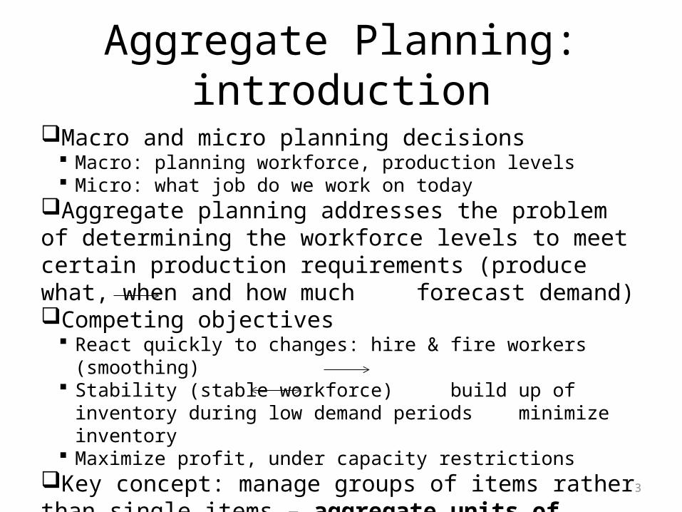
Aggregate Planning: introductionMacro and micro planning decisions

Macro: planning workforce, production levels Micro: what job do we work on today

Aggregate planning addresses the problem of determining the workforce levels to meet certain production requirements (produce what, when and how much forecast demand)Competing objectives

React quickly to changes: hire & fire workers (smoothing) Stability (stable workforce) build up of inventory

during low demand periods minimize inventory Maximize profit, under capacity restrictions

Key concept: manage groups of items rather than single items – aggregate units of production

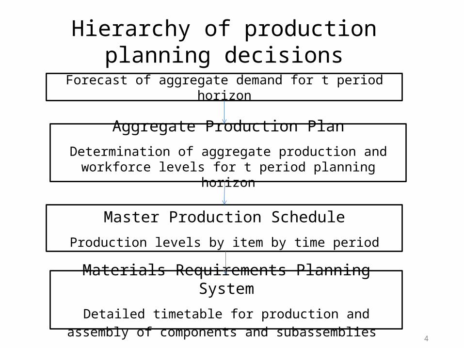
Hierarchy of production planning decisions

4

Forecast of aggregate demand for t period horizon

Aggregate Production Plan

Determination of aggregate production and workforce levels for t period planning horizon

Master Production Schedule

Production levels by item by time period

Materials Requirements Planning System

Detailed timetable for production and assembly of components and subassemblies

5

Aggregate units of productionAggregate planning assumes the existence of aggregate units of production

•‘Average unit’ (in case types of items are similar)•Aggregate units in terms of weights (tons of steel), volume, amount of work required sales ₤ volume …for different types of items•Families: Group of items that share a common manufacturing setup cost; i.e., they have similar production requirements.•Aggregate Unit: A fictitious item representing an entire product family.•Aggregate Unit Production Requirements: The amount of (labor) time required for the production of one aggregate unit.

Computing the Aggregate Unit Production Requirements - example

Washing machine Model Number

Required labor time (hrs)

Sales Volume ( %)

A5532 4.2 32

K4242 4.9 21

L9898 5.1 17

3800 5.2 14

M2624 5.4 10

M3880 5.8 06

Aggregate unit labor time = (.32)(4.2)+(.21)(4.9)+(.17)(5.1)+(.14)(5.2)+(.10)(5.4)+(.06)(5.8) = 4.856 hrs

7

Overview of the aggregate planning problem

What do we need?Demand (aggregate forecasts): assumption

‘known’ Aggregate units: considered ‘available’Planning horizon (6-12 months)CostsConstraints (e.g. bottlenecks, max capacity etc)

Planning Relationships

Business or annual plan

Planning Relationships

Business or annual plan

Production or staffing plan

Planning Relationships

MPS or workforce schedule

Business or annual plan

Production or staffing plan

Planning Relationships

MPS or workforce schedule

Business or annual plan

Production or staffing plan

Planning Relationships

MPS or workforce schedule

Business or annual plan

Production or staffing plan

Managerial Inputs

Supplier capabilities Storage capacity Materials availability

Materials

Current machine capacities Plans for future capacities Workforce capacities Current staffing level

Operations

New products Product design changes Machine standards

EngineeringLabor-market conditions Training capacity

Human resources

Cost data Financial condition of firm

Accounting and financeAggregate

plan

Customer needs Demand forecasts Competition behavior

Distribution and marketing

Aggregate Planning Objectives

• Minimize Costs/Maximize Profits• Maximize Customer Service• Minimize Inventory Investment• Minimize Changes in Production Rates• Minimize Changes in Workforce Levels• Maximize Utilization of Plant and

Equipment

Why Aggregate Planning Is Necessary

• Fully load facilities & minimize overloading and underloading

• Make sure enough capacity is available to satisfy expected demand

• Plan for orderly & systematic change of production capacity to meet peaks & valleys of expected customer demand

• Get most output for amount of resources available

• Given the demand forecast for each period in the planning horizon, we can determine the production level, inventory level, and the capacity level for each period that maximizes the firm’s (supply chain’s) profit over the planning horizon

• All supply chain stages should work together on an aggregate plan that will optimize supply chain performance

Role of Aggregate Planning in a Supply Chain

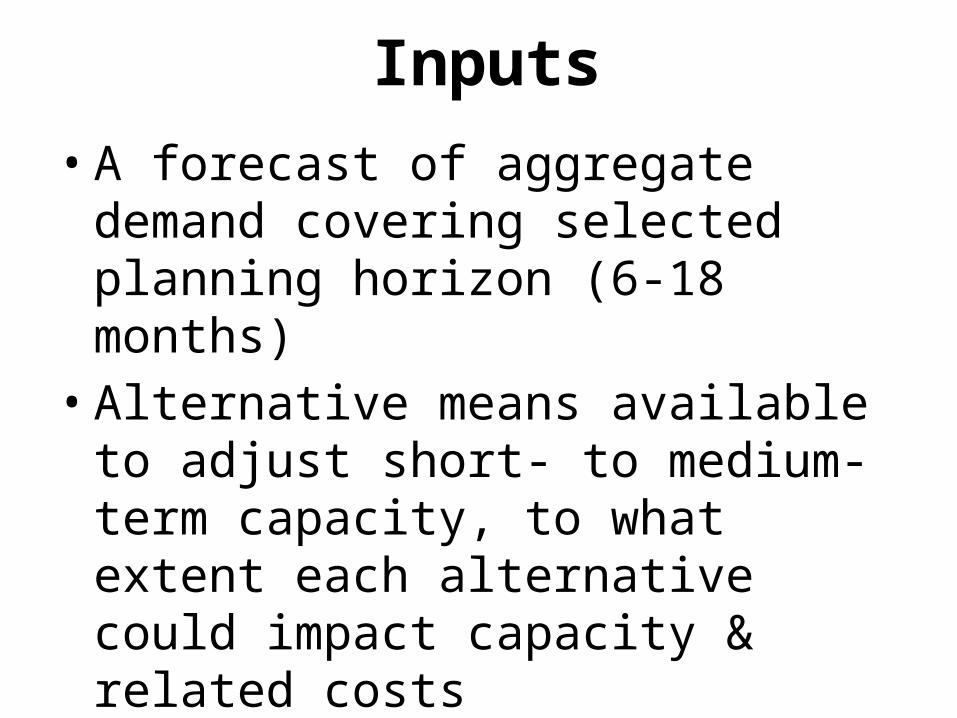
Inputs• A forecast of aggregate demand covering

selected planning horizon (6-18 months)• Alternative means available to adjust

short- to medium-term capacity, to what extent each alternative could impact capacity & related costs

• Current status of system in terms of workforce level, inventory level & production rate

Outputs

• Production plan: aggregate decisions for each period in planning horizon about– workforce level– inventory level– production rate

• Projected costs if production plan was implemented

Pure Strategies for Informal Approach

• Matching Demand (Chase Strategy)• Level Capacity

– Buffering With Inventory– Buffering With Backlog– Buffering With Overtime or Subcontracting

Matching Demand Strategy

• Capacity (production) in each time period is varied to exactly match forecasted aggregate demand in that time period

• Capacity is varied by changing workforce level• Finished-goods inventories are minimal• Labor & materials costs tend to be high due to

frequent changes

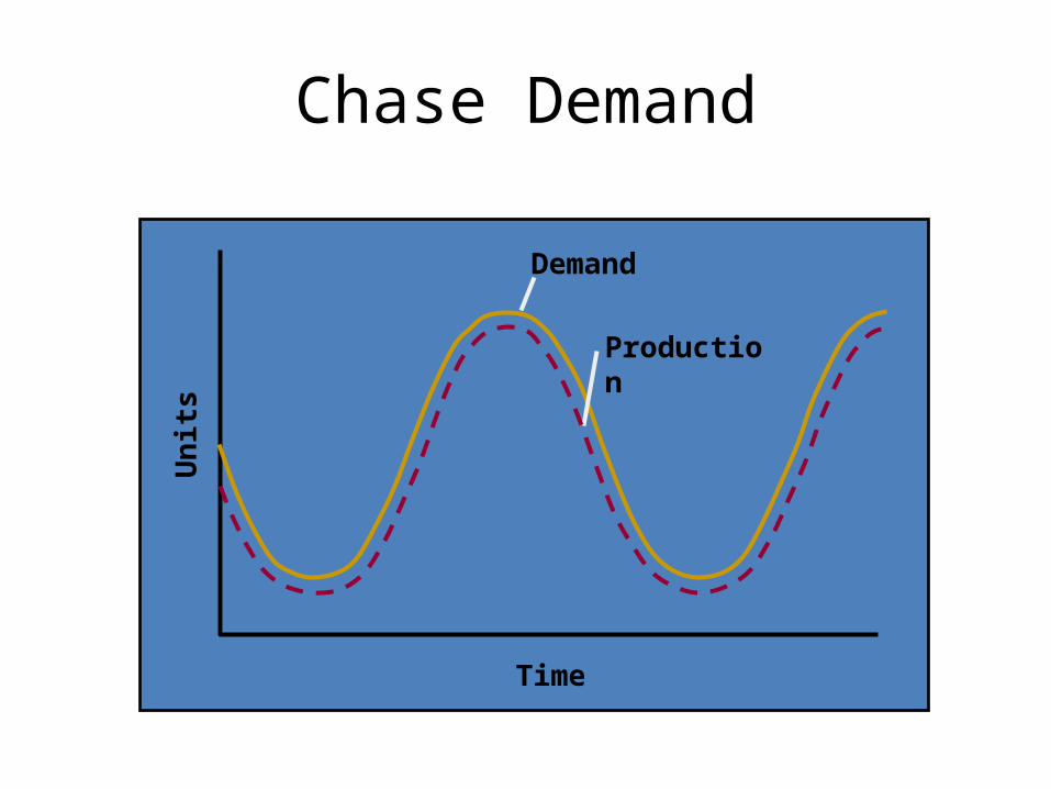
Chase Demand

Demand

Uni

ts

Time

Production

Developing & Evaluatingthe Matching Production Plan

• Production rate is dictated by forecasted aggregate demand

• Convert forecasted aggregate demand into required workforce level using production time information

• Primary costs of this strategy are costs of changing workforce levels from period to period, i.e.., hirings & layoffs

Level Capacity Strategy

• Capacity (production rate) is held level (constant) over planning horizon

• Difference between constant production rate & demand rate is made up (buffered) by inventory, backlog, overtime, part-time labor and/or subcontracting

Level Production

Demand

Uni

ts

Time

Production

Developing & EvaluatingLevel Production Plan

• Assume that amount produced each period is constant, no hiring or layoffs

• Gap between amount planned to be produced & forecasted demand is filled with either inventory or backorders, i.e., no overtime, no idle time, no subcontracting

• Primary costs of this strategy are inventory carrying & backlogging costs

Aggregate Planning StrategiesPossible Alternatives Possible Alternatives

Strategyduring Slack Season during Peak Season

1. Chase #1: vary workforce Layoffs Hiringlevel to match demand

2. Chase #2: vary output Layoffs, undertime, Hiring, overtime, rate to match demand vacations subcontracting

3. Level #1: constant No layoffs, building No hiring, depleting workforce level anticipation inventory, anticipation inventory,

undertime, vacations overtime, subcontracting, backorders, stockouts

4. Level #2: constant Layoffs, building antici- Hiring, depleting antici-output rate pation inventory, pation inventory, over-

undertime, vacations time, subcontracting, backorders, stockouts

Aggregate Planning Process

Figure 14.3

Determine requirements for planning horizon

Identify alternatives, constraints, and costs

Prepare prospective plan for

planning horizon

Move aheadto next

planning session

Implement and update the plan

Is the plan acceptable?

No

Yes

Aggregate Planning Costs

· Regular-time Costs· Overtime Costs· Hiring and

Layoff Costs· Inventory

Holding Costs· Backorder and Stockout Costs

Pure Strategies

Hiring cost = $100 per workerFiring cost = $500 per worker

Inventory carrying cost = $0.50 pound per quarter Regular production cost per pound = $2.00 Production per employee = 1,000 pounds per quarter Beginning work force = 100 workers

QUARTER SALES FORECAST (LB)

Spring 80,000Summer 50,000Fall 120,000Winter 150,000

Example:

Level Production Strategy

Level production

= 100,000 pounds(50,000 + 120,000 + 150,000 + 80,000)

4

Spring 80,000 100,000 20,000Summer 50,000 100,000 70,000Fall 120,000 100,000 50,000Winter 150,000 100,000 0

400,000 140,000Cost of Level Production Strategy(400,000 X $2.00) + (140,00 X $.50) = $870,000

SALES PRODUCTIONQUARTER FORECAST PLAN INVENTORY

Chase Demand Strategy

Spring 80,000 80,000 80 0 20Summer 50,000 50,000 50 0 30Fall 120,000 120,000 120 70 0Winter 150,000 150,000 150 30 0

100 50

SALES PRODUCTION WORKERS WORKERS WORKERSQUARTER FORECAST PLAN NEEDED HIRED FIRED

Cost of Chase Demand Strategy(400,000 X $2.00) + (100 x $100) + (50 x $500) = $835,000

Mixed Strategy

• Combination of level production and chase demand strategies

• Examples of management policies– no more than x% of the workforce can be laid off in one

quarter– inventory levels cannot exceed x dollars

• Many industries may simply shut down manufacturing during the low demand season and schedule employee vacations during that time

General Linear Programming (LP) Model

• LP gives an optimal solution, but demand and costs must be linear

• Let– Wt = workforce size for period t– Pt =units produced in period t– It =units in inventory at the end of period t– Ft =number of workers fired for period t– Ht = number of workers hired for period t

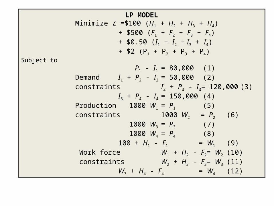
LP MODELMinimize Z = $100 (H1 + H2 + H3 + H4)

+ $500 (F1 + F2 + F3 + F4)+ $0.50 (I1 + I2 + I3 + I4)+ $2 (P1 + P2 + P3 + P4)

Subject toP1 - I1 = 80,000 (1)

Demand I1 + P2 - I2 = 50,000 (2)constraints I2 + P3 - I3 = 120,000 (3)

I3 + P4 - I4 = 150,000 (4)Production 1000 W1 = P1 (5)constraints 1000 W2 = P2 (6)

1000 W3 = P3 (7)1000 W4 = P4 (8)

100 + H1 - F1 = W1 (9) Work force W1 + H2 - F2 = W2 (10) constraints W2 + H3 - F3 = W3 (11)

W3 + H4 - F4 = W4 (12)

Other Quantitative Techniques

• Linear decision rule (LDR)• Search decision rule (SDR)• Management coefficients model

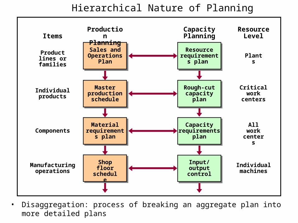
Hierarchical Nature of Planning

• Disaggregation: process of breaking an aggregate plan into more detailed plans

Items

Product lines or families

Individual products

Components

Manufacturing operations

Resource Level

Plants

Individual machines

Critical work centers

Production Planning

Capacity Planning

Resource requirements

plan

Rough-cut capacity

plan

Capacity requirements plan

Input/ output control

Sales and Operations

Plan

Master production schedule

Material requirements

plan

Shop floor schedule

All work centers