supply chain network structure and risk...
TRANSCRIPT

Supply Chain Network Structure and Risk Propagation
John R. Birge 1
1University of Chicago Booth School of Business (joint work with Jing Wu, Chicago Booth)
Kellogg School of Management, Northwestern U.
Birge (Chicago Booth) Supply Chain Structure October 1, 2014 1 / 27

Themes
Supply chain relationships have direct and indirect effects on firmperformance
Correlation and reliability issues in particular create nonlinear effects on thevalue of supplier connections
Effects of centrality on risk propagation can vary depending on position inthe supply chain
New databases (e.g., Bloomberg SPLC) provide opportunities to investigatefinancial and operational supply chain network interactions
Empirical results on firm returns show significant supplier and customereffects, lagged effects from supplier shocks, and differences in thesecond-order (systematic) risk impact of centrality depending on the firm’schain level
Birge (Chicago Booth) Supply Chain Structure October 1, 2014 2 / 27
Outline
Basic network configurations
Impact of nonlinearity on supply chain structure and risk propagation
Empirical data set
Analysis
Birge (Chicago Booth) Supply Chain Structure October 1, 2014 3 / 27

Example Relationships
Customer to Supplier: Calloway Golf/Coastcast Corporation (Cohen andFrazzini (2008))
Calloway reports earnings to be ∼half of expectations ($0.36 from $0.70)Calloway’s stock price drops 30%Coastcast share price (50% of sales to Calloway) virtually unchanged for overone monthAfter Coastcast announces lower earnings, price drop mirrors Calloway’s
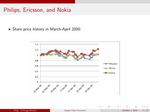
Supplier to Customer: Philips/Sony/Ericsson v. Nokia
Fire in Philips plant, key supplier for Nokia and Ericsson, in March 2000Initially, Philips states 1-week shutdown, then revises 2 weeks later (to 6weeks)Philips stock price drops then recoversNokia reacts quickly - earnings and share price riseEricsson reacts slowly - earnings and share price drop (with some delay)
Birge (Chicago Booth) Supply Chain Structure October 1, 2014 4 / 27

Calloway and Coastcast
From Cohen and Frazzini (2008):
Birge (Chicago Booth) Supply Chain Structure October 1, 2014 5 / 27

Calloway and Coastcast
From Cohen and Frazzini (2008):
Birge (Chicago Booth) Supply Chain Structure October 1, 2014 5 / 27

Calloway and Coastcast
From Cohen and Frazzini (2008):
Birge (Chicago Booth) Supply Chain Structure October 1, 2014 5 / 27

Calloway and Coastcast
From Cohen and Frazzini (2008):
Birge (Chicago Booth) Supply Chain Structure October 1, 2014 5 / 27

Calloway and Coastcast
From Cohen and Frazzini (2008):
Birge (Chicago Booth) Supply Chain Structure October 1, 2014 5 / 27

Philips, Ericsson, and Noka
Share price history in March-April 2000:
Birge (Chicago Booth) Supply Chain Structure October 1, 2014 6 / 27

Philips, Ericsson, and Noka
Share price history in March-April 2000:
Birge (Chicago Booth) Supply Chain Structure October 1, 2014 6 / 27

Philips, Ericsson, and Noka
Share price history in March-April 2000:
Birge (Chicago Booth) Supply Chain Structure October 1, 2014 6 / 27

Philips, Ericsson, and Noka
Share price history in March-April 2000:
Birge (Chicago Booth) Supply Chain Structure October 1, 2014 6 / 27

Philips, Ericsson, and Noka
Share price history in March-April 2000:
Birge (Chicago Booth) Supply Chain Structure October 1, 2014 6 / 27

Philips, Ericsson, and Nokia
Share price history in March-April 2000:
Birge (Chicago Booth) Supply Chain Structure October 1, 2014 7 / 27

Philips, Ericsson, and Nokia
Share price history in March-April 2000:
Birge (Chicago Booth) Supply Chain Structure October 1, 2014 7 / 27

Philips, Ericsson, and Nokia
Share price history in March-April 2000:
Birge (Chicago Booth) Supply Chain Structure October 1, 2014 7 / 27

Philips, Ericsson, and Nokia
Share price history in March-April 2000:
Birge (Chicago Booth) Supply Chain Structure October 1, 2014 7 / 27
Philips, Ericsson, and Nokia
Share price history in March-April 2000:
Birge (Chicago Booth) Supply Chain Structure October 1, 2014 7 / 27

Supply Chain Price Effects
Observations:Customer shocks are transmitted to suppliersSupplier shocks are also transmitted to customers (e.g., Hendricks and Singhal(2003))Historically, transmission has often been delayedAdaptive supply chains (e.g., alternate suppliers) can dampen shocks (andmay reduce risk exposures)
Share price effects:Model of price at time t:
pt =∑s
e−(rs+δ)sds
Expected dividends, ds , depend partly on supply chain partners (first-ordereffect)Risk premium, δ, depends on position in network and relationship ofconnections to risk transmission (second-order effect)
Impact of connection visibility:Changes in expectations may be delayed due to inattention or lack oftransparency into supply chain connections.
Birge (Chicago Booth) Supply Chain Structure October 1, 2014 8 / 27

Network Connections and Risk
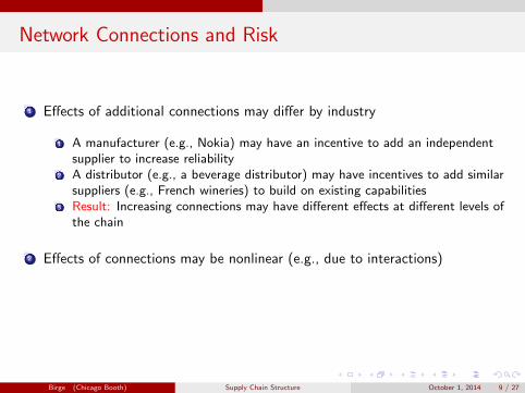
1 Effects of additional connections may differ by industry
1 A manufacturer (e.g., Nokia) may have an incentive to add an independentsupplier to increase reliability
2 A distributor (e.g., a beverage distributor) may have incentives to add similarsuppliers (e.g., French wineries) to build on existing capabilities
3 Result: Increasing connections may have different effects at different levels ofthe chain
2 Effects of connections may be nonlinear (e.g., due to interactions)
3 Nonlinear (joint firm) effects may be critical in the formation of supply chainlinks
Birge (Chicago Booth) Supply Chain Structure October 1, 2014 9 / 27

Network Connections and Risk
1 Effects of additional connections may differ by industry
1 A manufacturer (e.g., Nokia) may have an incentive to add an independentsupplier to increase reliability
2 A distributor (e.g., a beverage distributor) may have incentives to add similarsuppliers (e.g., French wineries) to build on existing capabilities
3 Result: Increasing connections may have different effects at different levels ofthe chain
2 Effects of connections may be nonlinear (e.g., due to interactions)
3 Nonlinear (joint firm) effects may be critical in the formation of supply chainlinks
Birge (Chicago Booth) Supply Chain Structure October 1, 2014 9 / 27

Network Model
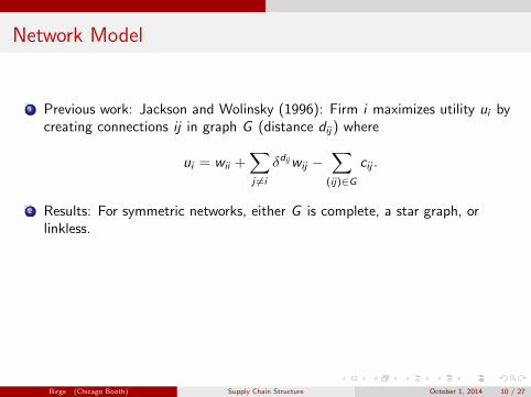
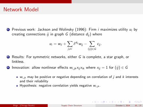
1 Previous work: Jackson and Wolinsky (1996): Firm i maximizes utility ui bycreating connections ij in graph G (distance dij) where
ui = wii +∑j 6=i
δdijwij −∑(ij)∈G
cij .
2 Results: For symmetric networks, either G is complete, a star graph, orlinkless.
3 Innovation: allow nonlinear effects wi,jkxijxik where xij = 1 for (ij) ∈ G
wi,jk may be positive or negative depending on correlation of j and k interestsand their reliabilityHypothesis: negative correlation yields negative wi,jk .
Birge (Chicago Booth) Supply Chain Structure October 1, 2014 10 / 27
Network Model
1 Previous work: Jackson and Wolinsky (1996): Firm i maximizes utility ui bycreating connections ij in graph G (distance dij) where
ui = wii +∑j 6=i
δdijwij −∑(ij)∈G
cij .
2 Results: For symmetric networks, either G is complete, a star graph, orlinkless.
3 Innovation: allow nonlinear effects wi,jkxijxik where xij = 1 for (ij) ∈ G
wi,jk may be positive or negative depending on correlation of j and k interestsand their reliabilityHypothesis: negative correlation yields negative wi,jk .
Birge (Chicago Booth) Supply Chain Structure October 1, 2014 10 / 27

Network Model
1 Previous work: Jackson and Wolinsky (1996): Firm i maximizes utility ui bycreating connections ij in graph G (distance dij) where
ui = wii +∑j 6=i
δdijwij −∑(ij)∈G
cij .
2 Results: For symmetric networks, either G is complete, a star graph, orlinkless.
3 Innovation: allow nonlinear effects wi,jkxijxik where xij = 1 for (ij) ∈ G
wi,jk may be positive or negative depending on correlation of j and k interestsand their reliability
Hypothesis: negative correlation yields negative wi,jk .
Birge (Chicago Booth) Supply Chain Structure October 1, 2014 10 / 27
Network Model
1 Previous work: Jackson and Wolinsky (1996): Firm i maximizes utility ui bycreating connections ij in graph G (distance dij) where
ui = wii +∑j 6=i
δdijwij −∑(ij)∈G
cij .
2 Results: For symmetric networks, either G is complete, a star graph, orlinkless.
3 Innovation: allow nonlinear effects wi,jkxijxik where xij = 1 for (ij) ∈ G
wi,jk may be positive or negative depending on correlation of j and k interestsand their reliabilityHypothesis: negative correlation yields negative wi,jk .
Birge (Chicago Booth) Supply Chain Structure October 1, 2014 10 / 27

Implications for Supply Chain Structure
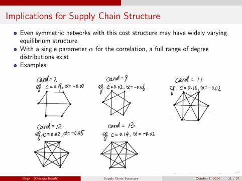
Even symmetric networks with this cost structure may have widely varyingequilibrium structureWith a single parameter α for the correlation, a full range of degreedistributions existExamples:
Birge (Chicago Booth) Supply Chain Structure October 1, 2014 11 / 27

Implications for Supply Chain Structure
Even symmetric networks with this cost structure may have widely varyingequilibrium structureWith a single parameter α for the correlation, a full range of degreedistributions existExamples:
Birge (Chicago Booth) Supply Chain Structure October 1, 2014 11 / 27
Implications for Supply Chain Structure
Even symmetric networks with this cost structure may have widely varyingequilibrium structureWith a single parameter α for the correlation, a full range of degreedistributions existExamples:
Birge (Chicago Booth) Supply Chain Structure October 1, 2014 11 / 27

Supply Chain Risk Propagation
Example framework: Suppliers A, B; manufacturer M; distributor/wholesaler W
A
B
tt
Mt WtZZZZ
����
Shocks: probability p of individual survival of each without considering theeffects of these nodes
Birge (Chicago Booth) Supply Chain Structure October 1, 2014 12 / 27

Risk Implications
Systematic risk: volatility of survival probability conditional on not having anidiosyncratic bad shock.
For each node in simple network: conditional survival probability p3.
Volatility =p3(1 − p3): decreases as p increases for p > 0.5.
Birge (Chicago Booth) Supply Chain Structure October 1, 2014 13 / 27

Expanded Network
Example framework: Suppliers Ai , Bi ; manufacturer Mi ; distributor/wholesaler Wi
A2
B2
tt
M2t W2tZZZZ
����
A1
B1
tt
M1t
����������
JJJJJJJ
W1tZZZZ
����
Figure: Example with four suppliers, two manufacturers, and two wholesaler/retailers.
Birge (Chicago Booth) Supply Chain Structure October 1, 2014 14 / 27

Propagation in Expanded Network
Manufacturer M1 can survive if one of the wholesaler nodes is wiped out;Wholesaler W2 cannot survive either manufacturer’s loss (due to lowermargin/market power).Implications:
More-connected M1’s conditional survival probability:
(1 − (1 − p)2)3 = p3(2 − p)3 > p3, (1)
where p3 is the conditional survival of the singly-connected M2.WholesalerW1’s conditional survival probability:
(1 − (1 − p)2)2p = p3(2 − p)2. (2)
W2’s conditional survival probability:
p4(2 − p)2 < p3(2 − p)2. (3)
Also, because p(2 − p)2 < 1,
p4(2 − p)2 < p3, conditional survival in simple tree. (4)
Result: Wholesaler/distributor with more connections faces higher risk whilethe opposite is true for manufacturers.
Birge (Chicago Booth) Supply Chain Structure October 1, 2014 15 / 27
Verifying Hypotheses Empirically
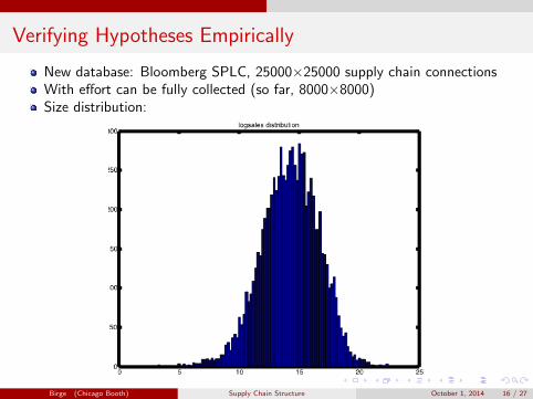
New database: Bloomberg SPLC, 25000×25000 supply chain connectionsWith effort can be fully collected (so far, 8000×8000)Size distribution:
Birge (Chicago Booth) Supply Chain Structure October 1, 2014 16 / 27

Verifying Hypotheses Empirically
New database: Bloomberg SPLC, 25000×25000 supply chain connectionsWith effort can be fully collected (so far, 8000×8000)Size distribution:
Birge (Chicago Booth) Supply Chain Structure October 1, 2014 16 / 27

Verifying Hypotheses Empirically
New database: Bloomberg SPLC, 25000×25000 supply chain connectionsWith effort can be fully collected (so far, 8000×8000)Size distribution:
Birge (Chicago Booth) Supply Chain Structure October 1, 2014 16 / 27

Verifying Hypotheses Empirically
New database: Bloomberg SPLC, 25000×25000 supply chain connectionsWith effort can be fully collected (so far, 8000×8000)Size distribution:
Birge (Chicago Booth) Supply Chain Structure October 1, 2014 16 / 27

Verifying Hypotheses Empirically
New database: Bloomberg SPLC, 25000×25000 supply chain connectionsWith effort can be fully collected (so far, 8000×8000)Size distribution:
Birge (Chicago Booth) Supply Chain Structure October 1, 2014 16 / 27

Degree distributions
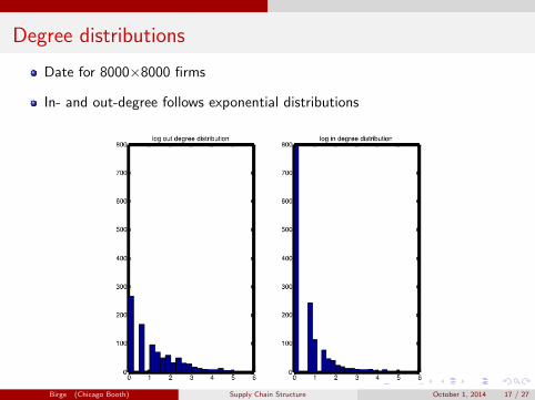
Date for 8000×8000 firms
In- and out-degree follows exponential distributions
Birge (Chicago Booth) Supply Chain Structure October 1, 2014 17 / 27
Degree distributions
Date for 8000×8000 firms
In- and out-degree follows exponential distributions
Birge (Chicago Booth) Supply Chain Structure October 1, 2014 17 / 27

Degree distributions
Date for 8000×8000 firms
In- and out-degree follows exponential distributions
Birge (Chicago Booth) Supply Chain Structure October 1, 2014 17 / 27

Degree distributions
Date for 8000×8000 firms
In- and out-degree follows exponential distributions
Birge (Chicago Booth) Supply Chain Structure October 1, 2014 17 / 27

Degree distributions
Date for 8000×8000 firms
In- and out-degree follows exponential distributions
Birge (Chicago Booth) Supply Chain Structure October 1, 2014 17 / 27

Example Connections
Top ten most connected firms:
Birge (Chicago Booth) Supply Chain Structure October 1, 2014 18 / 27

Example Connections
Top ten most connected firms:
Birge (Chicago Booth) Supply Chain Structure October 1, 2014 18 / 27

Example Connections
Top ten most connected firms:
Birge (Chicago Booth) Supply Chain Structure October 1, 2014 18 / 27

Example Connections
Top ten most connected firms:
Birge (Chicago Booth) Supply Chain Structure October 1, 2014 18 / 27

Example Connections
Top ten most connected firms:
Birge (Chicago Booth) Supply Chain Structure October 1, 2014 18 / 27

Supply Chain Relationship Hypotheses
Performance metric: stock return (proxy for direct shock effects andsystematic risk)
First-order effects (changes in future expectations of a firm)
Suppliers’ and customers’ concurrent performance relates to the firmSupplier momentum (one-month lag) may be related to firm performanceCustomer momentum (following Cohen and Frazzini (2008)) not related tofirm performance due to greater awareness
Second-order (systematic risk) effects (relationship to network connections)
Centrality influences firm risk and return performanceMore central manufacturing firms have lower returns (lower risk)More central logistics (transportation, wholesale, retail) firms have higherreturns (higher risk)
Birge (Chicago Booth) Supply Chain Structure October 1, 2014 19 / 27

First-Order Effects
Model:
ri,t = α + β1ri,t−1 + β2∑j
w inij rj,t−1 + β3
∑j
woutij rj,t−1
+β4∑j
w inij rj,t + β5
∑j
woutij rj,t + εi,t .
Coefficients α and βk , k = 1, . . . , 5 (estimated);∑
j winij rj,t−1 - one-month
supplier momentum,∑
j woutij rj,t−1 - one-month customer momentum,∑
j winij rj,t - concurrent supplier return, and
∑j w
outij rj,t - the concurrent
customer return.
Use US firms in SPLC.
Monthly returns over 2010-2012.
Include common risk factors (MKT, SMB, HML, MOM).
Birge (Chicago Booth) Supply Chain Structure October 1, 2014 20 / 27
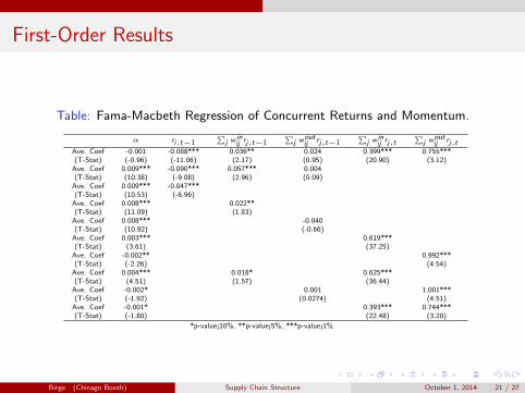
First-Order Results
Table: Fama-Macbeth Regression of Concurrent Returns and Momentum.
α ri,t−1∑
j winij rj,t−1
∑j w
outij rj,t−1
∑j w
inij rj,t
∑j w
outij rj,t
Ave. Coef -0.001 -0.088*** 0.036** 0.024 0.399*** 0.755***(T-Stat) (-0.96) (-11.06) (2.17) (0.95) (20.90) (3.12)Ave. Coef 0.009*** -0.090*** 0.057*** 0.004(T-Stat) (10.38) (-9.08) (2.96) (0.09)Ave. Coef 0.009*** -0.047***(T-Stat) (10.53) (-6.96)Ave. Coef 0.008*** 0.022**(T-Stat) (11.09) (1.83)Ave. Coef 0.008*** -0.040(T-Stat) (10.92) (-0.66)Ave. Coef 0.003*** 0.619***(T-Stat) (3.61) (37.25)Ave. Coef -0.002** 0.992***(T-Stat) (-2.26) (4.54)Ave. Coef 0.004*** 0.018* 0.625***(T-Stat) (4.51) (1.57) (36.44)Ave. Coef -0.002* 0.001 1.001***(T-Stat) (-1.92) (0.0274) (4.51)Ave. Coef -0.001* 0.393*** 0.744***(T-Stat) (-1.80) (22.48) (3.20)
*p-value¡10%, **p-value¡5%, ***p-value¡1%
Birge (Chicago Booth) Supply Chain Structure October 1, 2014 21 / 27

Supplier Momentum Strategy
Sort into quintiles of suppliers’ one-month lagged returns
Long on highest quintile and short on lowest
Approximately 0.6% excess return per month (∼7.5% annual)
Birge (Chicago Booth) Supply Chain Structure October 1, 2014 22 / 27

Supplier Momentum Strategy
Sort into quintiles of suppliers’ one-month lagged returns
Long on highest quintile and short on lowest
Approximately 0.6% excess return per month (∼7.5% annual)
Birge (Chicago Booth) Supply Chain Structure October 1, 2014 22 / 27

Supplier Momentum Strategy
Sort into quintiles of suppliers’ one-month lagged returns
Long on highest quintile and short on lowest
Approximately 0.6% excess return per month (∼7.5% annual)
Birge (Chicago Booth) Supply Chain Structure October 1, 2014 22 / 27

Supplier Momentum Strategy
Sort into quintiles of suppliers’ one-month lagged returns
Long on highest quintile and short on lowest
Approximately 0.6% excess return per month (∼7.5% annual)
Birge (Chicago Booth) Supply Chain Structure October 1, 2014 22 / 27

Supplier Momentum Strategy
Sort into quintiles of suppliers’ one-month lagged returns
Long on highest quintile and short on lowest
Approximately 0.6% excess return per month (∼7.5% annual)
Birge (Chicago Booth) Supply Chain Structure October 1, 2014 22 / 27

Second-Order Effects
Model:
Characterize centrality by eigenvector centrality and in- and out-degreecentralityUse average of industry if no relationship in datasetSplit by NAICS code (3 for manufacturing, 4 for logistics)
Split into quintiles of centrality.
Observe trends and significance in returns across quintiles.
Birge (Chicago Booth) Supply Chain Structure October 1, 2014 23 / 27

Second-Order Results: Manufacturing
Table: Factor Sensitivities by In-degree Centrality for Manufacturing Firms.
N3 Factor Loadings
Portfolio Alpha(%) Rmt − Rft SMB HML MOM Adj. R2(%)
1(Low) 0.340 1.250*** 92.13(0.99) (15.71)0.630* 1.119*** 0.327 -0.366 -0.145 93.25(1.81) (9.90) (1.17) (-1.68) (-1.27)
2 0.077 1.220*** 91.10(0.22) (14.70)0.414 1.085*** 0.491 -0.594** 0.025 93.63(1.25) (10.07) (1.85) (-2.86) (0.23)
3 0.430 0.902*** 86.05(1.26) (11.43)0.175 1.091*** -0.561* -0.205 0.079 87.74(0.50) (9.61) (-2.00) (-0.94) (0.69)
4 0.105 1.066*** 92.44(0.37) (16.05)0.127 1.098*** -0.079 -0.338 0.022 92.51(0.41) (10.83) (-0.31) (-1.73) (0.22)
5(High) 0.053 0.804*** 84.67(0.16) (10.81)-0.170 1.006*** -0.659*** -0.431** 0.009 91.00(-0.63) (11.52) (-3.05) (-2.56) (0.10)
High-Low -0.287*** -0.446***(-2.87) (-19.21)
-0.800*** -0.113*** -0.986*** -0.065 0.153***(-8.52) (-3.71) (-13.10) (-1.10) (5.03)
*p-value¡10%, **p-value¡5%, ***p-value¡1%
Birge (Chicago Booth) Supply Chain Structure October 1, 2014 24 / 27

Second-Order Results: Logistics
Table: Factor Sensitivities by In-degree Centrality for Logistics Firms.
N4 Factor Loadings
Portfolio Alpha(%) Rmt − Rft SMB HML MOM Adj. R2(%)
1(Low) 0.061 1.072*** 79.57(0.12) (9.10)-0.324 1.302*** -0.684 0.097 0.106 79.47(-0.58) (7.19) (-1.53) (0.28) (0.58)
2 0.327 1.078*** 80.94(0.72) (10.29)0.327 1.153*** -0.875** -0.065 -0.006 84.53(0.78) (8.87) (-2.72) (-0.26) (-0.04)
3 0.493 0.973*** 77.60(1.01) (8.59)0.242 1.142*** -0.427 -0.092 0.162 76.37(0.44) (6.40) (-0.97) (-0.27) (0.90)
4 0.703* 0.893*** 83.31(1.73) (9.50)0.741 0.888*** 0.737* -0.571* 0.101 86.72(1.67) (6.20) (2.08) (-2.07) (0.70)
5(High) 0.922** 0.638*** 75.37(2.71) (8.08)0.878** 0.735*** -0.140 -0.549** 0.202* 82.76(2.81) (7.26) (-0.56) (-2.81) (1.98)
High-Low 0.861*** -0.434***(6.60) (-14.37)
1.202*** -0.567*** 0.544*** -0.646*** 0.096**(8.80) (-12.82) (4.97) (-7.57) (2.15)
*p-value¡10%, **p-value¡5%, ***p-value¡1%
Birge (Chicago Booth) Supply Chain Structure October 1, 2014 25 / 27

Conclusions
1 Supply chain network connections link firms with direct and indirect effects
2 Nonlinear effects can allow for wide variation in topology
3 Risk propagation from connections varies depending on chain level
4 Data indicates wide range of degree distributions (that seem to imply somenonlinear relationships).
5 Evidence of concurrent supplier and customer effects plus suppliermomentum effects on returns.
6 Evidence of decreasing returns to centrality in manufacturing and increasingreturns to centrality in logistics.
Birge (Chicago Booth) Supply Chain Structure October 1, 2014 26 / 27

Thank you! Any questions?
Birge (Chicago Booth) Supply Chain Structure October 1, 2014 27 / 27