Supply Base Design for Innovative Items

Victor Martınez-de-Albeniz∗ Jiao Wang†

Submitted: October 25, 2017

Abstract

Sourcing innovative items in advance entails significant risks for the buyer. To reduce thepossibility of bringing a mediocre product to the market, buyers can build a large supply baseand pick the best available products after uncertainties have materialized. Designing such asupply base is a challenging task: the buyer needs to decide how many suppliers to recruit,and how to split them across potential categories, such as product types or geographies. Inthis paper, we propose a framework to design optimal supply bases when a certain amountof products are sourced from potential suppliers that are subject to uncertainties on theprofitability of their designs. We start with the case of independent supplier profits: wecharacterize the optimal supply base size and find that it is optimal to recruit a muchlarger number of suppliers compared to the number of products needed, which increases inthe riskiness of supplier designs so as to better exploit the potential upside in profitabilitydeviations. We then study the case where different supplier categories are correlated. Whilethe exact solution can be obtained in simple cases, the general stochastic problem can only besolved numerically. Hence we propose three approximations that provide excellent solutions,especially when the number of products to source is large. Our framework thus providesguidelines for buyers that want to diversify their sourcing risks through supply base design.

Keywords: Sourcing, supply base, excess capacity, order statistics

1 Introduction

One important building block of a sourcing strategy is to determine what are the potentialvendors eligible to provide supply. This set of suppliers is called the supply base (Choi andKrause 2006). When the items to be acquired do not vary much over time, the managementof the supply base can be relatively simple: decide the number of many potential vendors touse, and dynamically split the business among them (see Aoki and Lennerfors 2013 for a recentreview of Toyota’s practices). But when there is uncertainty in the sourcing market, buyers maywant to use more involved policies, such as pro-active qualification of new suppliers (Chaturvediet al. 2014).

Managing the supply base is even more complex when the products to be sourced are inno-vative: these are items that constantly change and as a result supplier competitive advantages

∗IESE Business School, University of Navarra, Barcelona, Spain, valbeniz@iese.edu. V. Martınez-de-Albeniz’sresearch was supported by the European Research Council - ref. ERC-2011-StG 283300-REACTOPS and by theSpanish Ministry of Economics and Competitiveness (Ministerio de Economıa y Competitividad) - ref. ECO2014-59998-P.

†Institute of Systems Engineering, Tianjin University, Tianjin, China and IESE Business School, University ofNavarra, Barcelona, Spain, jiaowang@tju.edu.cn

1

may not carry over to the next generation of products. For some products such as electronicparts, a supplier’s cost advantage today is likely to still result in a cost advantage tomorrow dueto technological or scale characteristics of that supplier. For those, costs are “sticky” so a stablesupply base would still be advisable. In contrast, there are many industries where innovationdoes not involve a functional improvement, such as new apparel products (Caro and Martınez-de Albeniz 2015). In these settings, product success and thus supplier competitive advantagesare more difficult to predict (Fisher 1997): effectively designing a supply base there becomes achallenging task that requires a good understanding of the risks and opportunities of bringingnew suppliers on board. On the one hand, maintaining an additional vendor increases the coststo the buyer, in the form of one-time or recurrent qualification procedures and audits. On theother hand, that additional supplier provides a real option to capture good ideas for futureproducts, which may become bestsellers. This real option may be quite valuable because thelarge spectrum of uncertainties and risks: from more predictable ones such as labor cost inflationto more uncertain ones such as exchange rate fluctuations, or even unpredictable shocks suchas sharp changes in political positions and trade agreements (Diamond 2017). Furthermore, in-novative items carry even more significant risks arising from the changing market demand, thatmay require rapidly updating product characteristics such as the material type in electronics orfashion apparel.

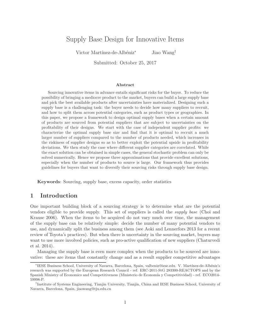
Consider for example the sourcing strategy of Inditex, the mother company of Zara andone of the world’s leading fast-fashion players. In 2015, Inditex used 1,725 suppliers running6,298 factories (p.32 in Inditex 2015; these suppliers sold at least 20,000 units to Inditex in2015). Maintaining such network of suppliers is a costly activity, given “the emphasis placed byInditex teams on ensuring traceability right up to the last link of the chain” and that “Inditex isalso working hard on the identification of raw materials”, e.g., it “works with the major globalsuppliers of forest-based artificial fibres such as viscose, modal and lyocell to ensure that onlyfibre complying with this policy is used in the products sold by Inditex.” However, given thatInditex specializes in quickly following fashion trends, it also needs to include a wide range ofcategories and styles of items into the assortment, which are updated periodically. These itemsproduced by the suppliers distributed across the European Union, the rest of Europe, Asia,Africa and the Americas (see Figure 1). Exploiting the opportunities of such a global supplybase thus requires carefully understanding the differences across these geographies, which areaffected by different dynamics, as well as the many other relevant dimensions to apparel sourcingsuch as product types and manufacturing technologies. We can thus envision the complexityof designing a supply base strategy for a company like Inditex: How many suppliers should bequalified in each category (e.g., region and product type)? How should the business be allocatedto them over time?

In this paper we propose a simple framework to support supply base design decisions. Weseparate the decision process in two phases. First, the buyer builds the supply base, which willremain stable for several future periods, e.g., 3-5 years in apparel sourcing. This decision willbe to determine how many suppliers to include in each possible category, e.g., regions. Then, ineach period, risks are materialized, e.g., fashion trends like pantsuits or fur for Fall-Winter 2017(Hua 2016). At that point, the buyer can explore the supply base to obtain the best designsavailable, those with the highest sales potential. Of course, the more diversified the supply base,the wider the choice for the buyer and hence the higher the profits. Specifically, we assume thatin each period a fixed number of designs Q can be brought to market (one design is providedby one supplier), and that supplier profitabilities are the outcome of random variables; thesemay be correlated within each category, because of the common risks affecting them. Althoughour model assumes that the profit captured by the buyer is equal to the realization of the

2

!"#$%&'(#() !*+

1410 factories !"#$%,(&-(.#(+

2086 factories

/0".1,+

316 factories

/2.,+

2252 factories

/3%".1,+

234 factories

Figure 1: The distribution and number of active factories for Inditex, adapted from Inditex(2015).

random variables, we also show how to incorporate endogenous prices, which does not changethe structure of the problem (see Babich et al. 2007 or Wan and Beil 2014 for such modelswith endogenous prices). Our framework is thus a mathematical program which includes a largenumber of stochastic elements and a possibly complex correlation structure.

We start analyzing the case of uncorrelated profitabilities, so that ex-ante all suppliers providethe same profitability. In this case, there are no categories to worry about and only the totalnumber of suppliers matters. The solution to our decision problem provides the optimal “excessdesign capacity” that the buyer should plan for: indeed, it is better to build a large supply baseto generate more variability in the design profitabilities, so as to pick the highest potentials andincrease the upside deviation. We find that the size of the optimal supply base decreases withper-supplier costs and increases with the number of items to be produced and the uncertaintyof each design. This case is similar to the standard supply base problem (Wan and Beil 2009),but with multiple winners. The resulting analysis is hence more complex but we show that it isstill tractable.

We then extend our model to the case of correlated profitabilities within each category.This case becomes significantly harder to model and analyze, yet it captures a key driver ofdiversification decisions and has not been explored in the literature before. We propose aparticular separation of supplier profitabilities that allows us to formulate the problem in acompact fashion: the profitability of suppliers in a given category is written as the sum of acategory effect common to all the corresponding suppliers, plus a supplier-specific shock. Whenthe buyer only needs to source one product per period, we show that the optimal solution canbe obtained in closed form. In contrast, when multiple products are needed, then the optimalsolution cannot be characterized exactly. We thus develop one upper bound, based on the dualproblem, and two lower bounds, which are written as simpler stochastic allocation problems,without correlation. The approximations are then tested in a large numerical study. We findthat higher correlation within a category decreases the optimal amount of suppliers included init, which is in line with the intuition that more variability leads to larger supply bases. We alsoobserve that the three bounds are generally quite tight when the number of products to source(Q) is large, and one of the lower bounds provides near-optimal solutions.

This paper thus makes several contributions to the sourcing literature. First, we provide atractable analysis of the qualification problem with multiple winners, which is usually difficult

3

(Chaturvedi 2015) because it involves manipulating multiple order statistics. Indeed, our anal-ysis extensively uses order statistics techniques and in particular a recursive formulation thatrelates the expectation of k-th highest and k + 1-th highest order statistics of the profits. Forsome well-known distributions such as uniform, exponential or Pareto, these techniques allow usto write the buyer’s net expected profit into a compact expression, with only the expectation ofthe highest order statistic inside. Second, we include a correlation structure between suppliers,which is rare in the literature because it enormously complicates the analysis. We neverthelessshow how to find optimal solutions in some cases (Q = 1) and provide effective solutions ingeneral (Q > 1).

The remainder of this paper is organized as follows. In §2, we review the related literature.The model is described in §3. Results for the independent and correlated cases are shown in §4and §5 respectively. In §6, we present a large numerical study in which the performance of theapproximations is examined. We conclude in §7. All the proofs are included in the Appendix.

2 Literature review

This paper is mainly related to two streams of research. First, our model falls within thesourcing works in both operations management and economics. Second, our solution methodsrequire using properties found in the order statistics works.

2.1 Sourcing

There is a large body of research on sourcing and supply base design in operations management.Indeed, sourcing is one of the central decisions for the operations function. These decisions areoften made under uncertainty, which might come from the demand and/or supply side. Thenewsvendor model has been the traditional approach to incorporate demand uncertainty in thedecision process (Zipkin 2000). Many variations of the model have been proposed, includingcontracting to align supply chain partners (for a review see Cachon 2003), multiple events inwhich more information is acquired (Heath and Jackson 1994, Gallego and Ozer 2001, Songand Zipkin 2012) or planning of flexible capacity (Martınez-de-Albeniz and Simchi-Levi 2005,Allon and Van Mieghem 2010), to cite only a few. In addition, uncertainties in the supply sidehave also been explored, regarding production cost (Kalymon 1971, Golabi 1985, Berling andMartınez-de Albeniz 2011, Cakanyıldırım et al. 2012) or supply reliability (Parlar and Wang1993, Ciarallo et al. 1994, Parlar 1997, Tomlin 2006, Dada et al. 2007, Yang et al. 2012, Snyderet al. 2016).

To deal with these uncertainties, two popular approaches have been proposed. First, one canbuild additional supply, in the form of safety stock or excess capacity, so that abnormally highdemand can be served. The amount of safety is typically determined by the balance betweenproduct margins (lost when supply is insufficient) and costs (to be paid even when the itemcannot be sold). Second, one can also diversify the sources of supply, to reduce their aggregateuncertainty. These two levers are complementary, but aligning them optimally requires a carefulunderstanding of the correlation structure between supplier uncertainties. There are three papersthat have explicitly incorporated correlation into the diversified sourcing problem. Babich et al.(2007) discuss how to allocate ordering quantities among suppliers with correlated default risks,in a model with endogenous prices. They show that the buyer prefers factories with positivelycorrelated default risks despite the loss of diversification benefits because default risk correlationincreases supplier competition. Wan and Beil (2014) consider auctions with suppliers in differentcategories, with within-category common shocks. They study the buyer’s optimal diversification

4

decision and show that correlation within the categories forces the buyer to seek diversificationwithin each category to avoid local monopoly power. The third related work is Chaturvedi andMartınez-de Albeniz (2016), which do not consider endogenous prices but provide a tractableuncertainty framework to include correlation, and show that optimal diversification decreaseswith correlation.

In our model, we analyze the sourcing problem where each potential supplier can at mostdeliver one item. The supply base design problem is similar to that of Wan and Beil (2014)with the difference that the buyer requests multiple items and hence multi-sourcing is necessary.Note that although our price mechanism is exogenous in our main model, it can be readilyextended to endogenous uniform pricing (see our Equation 5). Furthermore, we provide a generalframework that can handle large number of suppliers, in the spirit of Chaturvedi and Martınez-deAlbeniz (2016). For this purpose, we develop new effective approximations to quickly optimizediversification across multiple supplier categories.

Finally, our work is also related to auction theory to some extent. Specifically, some ofour results are connected to one of the most famous and salient theorems in auction theory,the revenue equivalence theorem. It was first established among classical auction mechanisms(the first-price sealed auction and second-price auction) by Vickrey (1961) and later generalizedto a quite general case by Myerson (1981). It states that the seller’s expected utility underdifferent auction mechanisms are the same provided that the base utilities are the same (thatobtained by the low types). In our paper, Lemma 1 with k = 1 provides a similar result tothat of Myerson (1981), so that the expected revenue for a first-price auction is equivalent tothe expected second-price value realization; we use it for larger values of k, i.e., we relate theexpected k + 1-th random variable to that of the k-th random variable that follows a differentdistribution.

2.2 Order statistics

The analytical approaches used in this paper are related to the works on order statistics. Indeed,in our model we show that deriving the expected profit from sourcing Q items is in fact just thesame as deriving the expectation of the linear combination of the first Q-highest order statistics.

The distribution of order statistics of independent and identically distributed variables is wellknown, we thereby only discuss the works on correlated variables. It is technically difficult toderive the distribution and the moments of the linear functions of order statistics directly whenthe random variables are correlated. Wiens et al. (2006), Arellano-Valle and Genton (2007) andJamalizadeh and Balakrishnan (2010) make some attempts on this, but all these papers assumethat the joint distribution of all the random variables is known, which is either multivariatenormal or unified skew-elliptical distributions.

To avoid this problem, we derive the distribution and expectation of each order statistic firstand then calculate the distribution and expectation of the linear function of order statistics.Owen et al. (1962) first derives the moments of order statistics from equi-correlated multivariatenormal distribution. Rawlings (1976) and Hill (1976) investigate the formulae for the expectedvalues of order statistics of observations which comprise a number of equally-sized groups ofindividuals in which group members are correlated. We follow the way of Hill (1976) in char-acterizing the correlation among the variables, i.e., assuming the profit of each item being in aadditive form, the sum of one common term and one specific term. In contrast to Hill (1976)and other works on this, we do not necessarily assume that the variables follow multivariatenormal distribution, and specifically also consider uniform or exponential distributions. In ad-dition, besides studying the effect of the intra-set correlation on the first moment of k-th order

5

statistics, we derive approximations so that we can decide the optimal number of factories ineach category in the general case, when the exact problem is untractable.

3 Model description

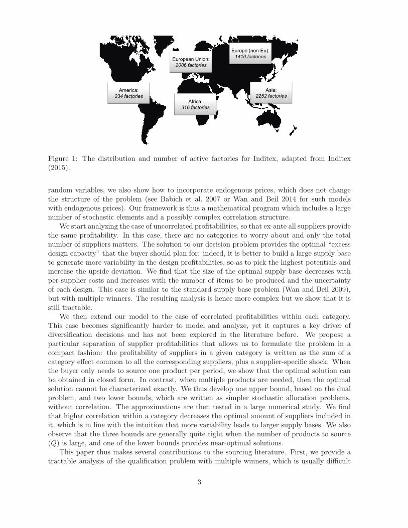
We consider the sourcing strategy problem of one large buyer such as Inditex, as described in theintroduction. There are two main phases that this buyer must consider: first there is a planningphase which aims at designing the supply base; second there is an execution phase which assignsfactories to production in each of the planning periods. Figure 2 illustrates the two phases.�������� ������� ���� ���� ���������� ������������������������� ����� �������

���� ���������� �������� �������� ����� ������������Figure 2: Model structure

Specifically, at the beginning of the horizon, the buyer must decide which factories to makeeligible for future work, for the entire horizon. This is a standard procedure at least in ap-parel sourcing, such as for Inditex and H&M. Denote the number of factories to use in eachcategory m = 1, 2 . . . ,M by Nm. m can represent a geographical category as in Figure 1, or aproduct-expertise pool. Categories are defined such that all factories in the same group sharea common uncertainty, and factories within the same category are independent of each other.For example, the economic environment in a given region, that includes factors such as politicalrisk, exchange rate fluctuations, labor cost changes, regional industry development or nationalindustrial policies, may be quite uncertain and affect all factories in that region (Wan and Beil2014).

We assume that all factories are homogeneous in capacity: each one can produce one item perperiod at most (i.e., has a capacity of one item per period). Of course, this simplified assumptionis made for tractability and may not be always satisfied. More generally, if a factory can produceseveral items in a period, our model could incorporate this feature by adding one more layer ofdecision variables, where the capacity at each factory should be determined. This complicatesthe exposition and the analysis due to more complex correlations and numerous configurationsof factories’ competitive advantages. So our choice of homogeneous factories makes the analysistractable and is sufficient to uncover the main trade-offs around supplier correlations.

Entering into one category may require significant expenses. For instance, if the categoriesare regions, entering a new geography entails negotiating with the local governments, obtainingadministrative licences, investing in new business structures, etc. To make an informed decision,the buyer usually will also spend a fair amount of time to screen and evaluate the factories inthe category beforehand (Wan and Beil 2009). All these activities will result in a variable costfor each supplier in the category, which is denoted by cm. This cost can also be a set-up cost

6

that has to be paid for each new factory the buyer qualifies. It may include the cost of audits,supplier tests and general investments in machinery for that supplier before placing any order.The value of cm may of course vary across categories due to different labor laws and practices,automation level or government regulation. In most of our analytical results, we assume fortractability that cm = c, i.e., homogeneous categories.

Once the supply base has been determined, there are T periods (e.g., fashion seasons Spring-Summer and Fall-Winter) in which the buyer chooses what to produce, and where to sourcefrom. We assume that in period t, Qt different items are required by the market. In that period,the profit for the buyer induced by selecting factory jm = 1, . . . , Nm in category m = 1, . . . ,Mis denoted by Zmjmt. It is assumed to be the sum of Xmt and Ymjmt, i.e., Zmjmt = Xmt+Ymjmt,where both Xmt ≥ 0 and Ymjmt ≥ 0 are random variables that will not be realized untilthe beginning of period t. Specifically, consistent with our definition of the categories, {Xmt}represent the common uncertainty in category m and are independent across m = 1, . . . ,M andt = 1, 2, . . . , T . We let the cumulative distribution function (c.d.f.) of Xmt be Fm to makeexposition simpler (although our approach can also capture situations where Xmt is seriallycorrelated over time). Furthermore, {Ymjmt} capture the factory-specific shocks in period t,which are also independently distributed and follow a c.d.f. Gm. Such additive form to modelcorrelation across factories is assumed on one hand because of its explicit separation of categoryand individual factory effects, and on the other hand for tractability (a multiplicative form wouldbe equally easy to manage). It has been used before, e.g., in Hill (1976), Wan and Beil (2014)and Chaturvedi and Martınez-de Albeniz (2016).

Further, it is worth noting that given that all the uncertainties have been realized at thestart of period t, the buyer merely needs to sort the profits of all the items in decreasing orderand pick from the highest one to the one that makes the total number of items picked reach Qt.This is because at the time the buyer periodically decides which factories in the supply base willbe active in period t, the costs cm are already sunk costs. Therefore, the buyer’s decision onlydepends on the realized profits of sourcing from each supplier. We define the expected profitachieved in one such period as:

R(

Qt, {Xmt}, {Ymjmt})

= maxzmjmt

M∑

m=1

Nm∑

jm=1

zmjmt(Xmt + Ymjmt)

s.t.

Nm∑

jm=1

zmjmt ≤ Nm,

M∑

m=1

Nm∑

jm=1

zmjmt ≤ Qt,

0 ≤ zmjmt ≤ 1, for m = 1, . . . ,M and jm = 1, . . . , Nm.(1)

The problem in (1) is a simple linear program (LP) over the simplex with capacity constraints(in particular, the constraint matrix is totally unimodular hence the optimal solution is integer).Besides, since the distributions of Xmt and Ymjmt (Fm and Gm respectively) are independentof time, the buyer’s assignment problem is the same in every period. Thus, we only focus onthe optimization of the first stage, the supply base design problem, assuming optimal executionin periods t = 1, 2, . . . , T . Hence, below the subscript t of {Xmt} and {Ymjmt} will be omitted.Suppose the maximum number of items to be requested in the second phase is Q. Therefore,

7

the buyer’s planning problem in the first stage can be expressed as

π∗ = maxN1,...,Nm≥0

π(N1, . . . , NM ) := E[R(Q, {Xm}, {Ymjm})]−

M∑

m=1

cmNm. (2)

There may be other possible interpretations for (2). For example, the number of categoriesand the number of suppliers in our case can be seen as the number of manufacturers and thenumber of items to procure from, respectively. In that case, Xm + Ymjm will be the profit madefrom the item jm designed by factory m; the cost cm can be explained as reservation cost. Andthe buyer’s problem is to decide how many items should be reserved from each manufacturerbeforehand and then then select the requested number of items from these reserved items.1

To further characterize the buyer’s decision in phase 1, denote the kth highest order statisticof the profits from all the possible

∑Mm=1Nm items by Z(k). As a result, the buyer’s expected

profit in phase 1 can also be written as

Q∑

k=1

E

[

Z(k)]

−

M∑

m=1

cmNm (3)

and hence the buyer’s problem turns into

maxN1,...,NM≥0

Q∑

k=1

(∫ ∞

0HZ(k)(z)dz

)

−M∑

m=1

cmNm (4)

where HZ(k) is the c.d.f. of Z(k) and HZ(k) is its complement.Before proceeding into the analysis, note that the formulations in (2) and (4) assume that

information is publicly revealed and that the buyer knows the true profits that can be extractedfrom each factory. In reality, there may be private information on the hands of the individualfactories and they may want to quote a price higher than cost. In that case, if the profits fromall the factories are independent with each other, the buyer could run a multi-object uniform-price auction at the beginning of each period,2 in which the factories with the first Q highestXm + Ymjm would be selected, but the buyer would only receive a profit equal to Q timesthe profit from the highest non-selected factory (that of the Q + 1 highest profit, which is themarginal factory which determines the uniform price paid to all the winners). Correspondingly,the objective of the buyer in the first phase under this situation would be

maxN1,...,NM≥0

π(N1, . . . , NM ) = Q

∫ ∞

0HZ(Q+1)(z)dz −

M∑

m=1

cmNm. (5)

We can see that the structure of the problem remains similar to that of (4). Thus, in theremainder of the paper we show our results for (4), although they can be extended to thealternative formulation (5).

To make exposition easier, we assume that the following two assumptions will hold.

1One example for this kind of sourcing is illustrated in Tokatli (2008): Zara first develops a relationship witha large number of suppliers in different countries according to the strategic plan of supply chain development ofthe company; and then the suppliers will visit Zara in Spain every 3-4 weeks presenting collections of 20-30 itemseach time; based on the style, quality and cost, etc., Zara then makes a purchasing decision.

2It does not matter if the buyer runs a discriminating auction since according to Harris and Raviv (1981), theauctioneer’s expected revenues will be the same under these two kinds of auction mechanisms when the biddersare risk neutral and have independent identical distributed valuations.

8

Assumption 1. The failure rate of Ymjm satisfies 1−G(z)g(z) = α+ βz.

Assumption 2. The increase of 1−G(z)g(z) is less than linear, i.e., β ≤ 1.

The failure rate of several quite common distributions actually can be rewritten into theform in Assumption 1 and also satisfy Assumption 2, with α and β being two constants thatvary with the specific distributions. For example, if Ymjm are uniform, or exponential or Paretodistributions with finite mean, then both Assumptions 1 and 2 are satisfied (details on this areprovided later in Table 1). Finally, although these are strong assumptions, note that almost allour results remain true when more general distributions are used, as we comment below.

Before proceeding with the results, note that when the buyer sources from one category only,i.e., M = 1, the common economic environment of the factories does not affect the assignmentwithin the supply base and hence does not influence the optimal Nm. We can thus assumein this case that Xm ≡ 0 and the profits of all the items become independent. However, ingeneral, when there is more than one category M > 1, correlation among profits of the itemsfrom the same category cannot be ignored, and the analysis becomes more complicated. Hence,we present the results first for the case with independent profits in §4 and then the correlatedone in §5. Further, since it is much simpler to analyze the case of one item (Q = 1) than that ofmultiple items (Q > 1), especially when M > 1, we will discuss these two situations separatelyin the correlated case.

4 Independent profits

From (4), to derive the buyer’s optimal supply base design, we must at first calculate thedistribution functions of the order statistics:

∑Qk=1 E

[

Z(k)]

=∑Q

k=1

(∫∞

0 HZ(k)(z)dz)

.From David and Nagaraja (2003), we know that if Ymjm are independent and identically

distributed variables, then the c.d.f. of Z(k), the k-th order statistics of Ymjm is

HZ(k)(z) =k∑

i=1

(

N

i− 1

)

G(z)N−i+1[1−G(z)]i−1. (6)

Substituting (6) into∫∞

0 HZ(k)(z)dz, the expectation of k-th order statistics can be derived.Interestingly, we find that there is a recursive formulation that relates the expectation of (k+1)-th order statistics to that of k-th order statistics, which is given by the the following lemma.

Lemma 1. E

[

Z(k+1)]

= E

Z(k) −1−G

(

Z(k))

kg(

Z(k))

.

Lemma 1 will be of great importance in our analysis. Note that in the particular case k = 1,it leads to the revenue equivalence theorem from Myerson (1981) or Milgrom and Weber (1982):

E[

Z(2)]

= E

[

Z(1) − 1−G(Z(1))

g(Z(1))

]

. This is equivalent to saying that in a first-price auction where

bidders submit profit-maximizing bids, the auctioneer’s expected profits are the same as that ina second-price auction.

What is more, it is worth noting that given that the profit distributions of the items satisfyAssumption 1, i.e., 1−G(z)

g(z) = α+ βz, the recursive equation in Lemma 1 turns into

E

[

Z(k+1)]

= −α

k+

(

1−β

k

)

E

[

Z(k)]

,

9

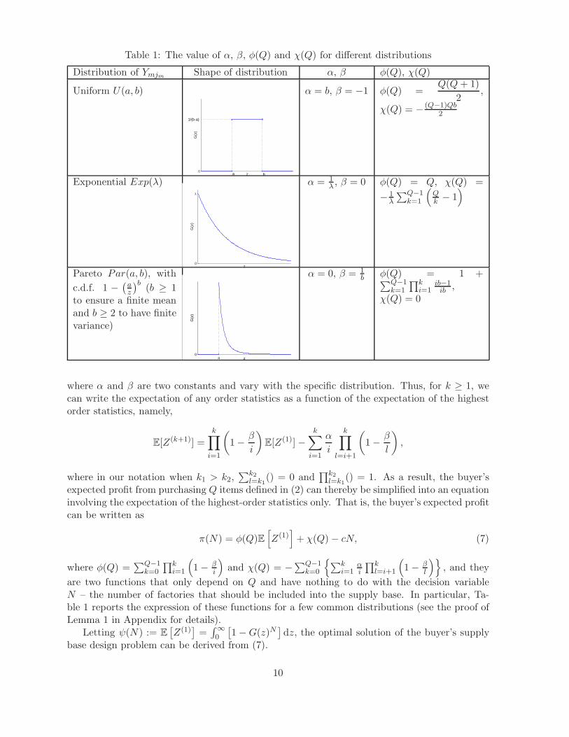
Table 1: The value of α, β, φ(Q) and χ(Q) for different distributions

Distribution of Ymjm Shape of distribution α, β φ(Q), χ(Q)

Uniform U(a, b)

z

G(z

)

0ba

1/(b-a)

α = b, β = −1 φ(Q) =Q(Q+ 1)

2,

χ(Q) = − (Q−1)Qb2

Exponential Exp(λ)

z

G(z

)

0

λ

α = 1λ , β = 0 φ(Q) = Q, χ(Q) =

− 1λ

∑Q−1k=1

(

Qk− 1)

Pareto Par(a, b), with

c.d.f. 1 −(

az

)b(b ≥ 1

to ensure a finite meanand b ≥ 2 to have finitevariance)

za

G(z

)

0

α = 0, β = 1b φ(Q) = 1 +

∑Q−1k=1

∏ki=1

ib−1ib ,

χ(Q) = 0

where α and β are two constants and vary with the specific distribution. Thus, for k ≥ 1, wecan write the expectation of any order statistics as a function of the expectation of the highestorder statistics, namely,

E[Z(k+1)] =

k∏

i=1

(

1−β

i

)

E[Z(1)]−

k∑

i=1

α

i

k∏

l=i+1

(

1−β

l

)

,

where in our notation when k1 > k2,∑k2

l=k1() = 0 and

∏k2l=k1

() = 1. As a result, the buyer’sexpected profit from purchasing Q items defined in (2) can thereby be simplified into an equationinvolving the expectation of the highest-order statistics only. That is, the buyer’s expected profitcan be written as

π(N) = φ(Q)E[

Z(1)]

+ χ(Q)− cN, (7)

where φ(Q) =∑Q−1

k=0

∏ki=1

(

1− βi

)

and χ(Q) = −∑Q−1

k=0

{

∑ki=1

αi

∏kl=i+1

(

1− βl

)}

, and they

are two functions that only depend on Q and have nothing to do with the decision variableN – the number of factories that should be included into the supply base. In particular, Ta-ble 1 reports the expression of these functions for a few common distributions (see the proof ofLemma 1 in Appendix for details).

Letting ψ(N) := E[

Z(1)]

=∫∞

0

[

1−G(z)N]

dz, the optimal solution of the buyer’s supplybase design problem can be derived from (7).

10

Theorem 1. (i) When M = 1, N∗ is determined by an integer above or below the solutionto

ψ′(N∗) = −

∫ ∞

0G(z)N

∗

lnG(z)dz =c

φ(Q); (8)

(ii) The buyer’s expected profit is submodular in N and c;

(iii) The buyer’s expected profit is supermodular in N and Q.

Note that the left-hand side of (8) is the marginal benefit of adding a new factory and theright-hand side of (8) is the corresponding marginal cost. Hence, the basic logic behind thebuyer’s optimal decision is to increase the number of factories until the marginal benefit is equalto the marginal cost. For instance, when Q = 1, the optimal solution is determined by theinteger above or below the solution to −

∫∞

0 G(z)N∗lnG(z)dz = c. Therefore, compared with

the case of requesting only one item, it can be seen that the information from Q is condensedso that it directly affects the marginal cost c/φ(Q). Further, as φ(Q) is no less than 1 due toβ ≤ 1, more factories will be used when requesting multiple items than when only sourcing oneitem. Moreover, from the second and third part of Theorem 1 we can conclude that with eitherthe decrease of the variable cost or the increase of the number of items to be requested, theoptimal number of factories will increase.

The properties illustrated above hold not only for the distributions that satisfy Assumptions1 and 2, but also for more general distributions. Given any distribution G, substituting thedistribution of the order statistics (6) into (4), the buyer’s problem can be rewritten as

maxN≥0

π(N) =

Q∑

k=1

∫ ∞

0

{

1−

k∑

i=1

(

N

i− 1

)

G(z)N−i+1[1−G(z)]i−1

}

dz − cN, (9)

from which the buyer’s optimal decision therefore can be derived and is characterized by thefollowing theorem.

Theorem 2. When M = 1, if Yjm follow i.i.d. general distributions, then

(i) N∗ is determined by the largest integer that satisfies

Q∑

i=1

(Q+ 1− i)

∫ ∞

0G(z)N+1−i[1−G(z)]i−1

(

N

i− 1

){

1−N + 1

N − i+ 2G(z)

}

dz ≥ c; (10)

(ii) the buyer’s expected profit is submodular with respect to N and c;

(iii) the buyer’s expected profit is supermodular with respect to N and Q as long as

∫ ∞

0G(z)N+1−i[1−

G(z)]i−1

(

N

i− 1

){

1−N + 1

N − i+ 2G(z)

}

dz ≥ 0 holds.

Once again, the left-hand side of (10) in part (i) of Theorem 2 is the marginal benefit ofadding a new factory and the right-hand side is the marginal variable cost. Hence, the buyerwill keep adding new factories into the supply base until the marginal benefit is less than thecost c. Noting that the left-hand side of (10) is decreasing in N . Therefore, the optimal numberof factories N∗ is non-increasing in c, i.e., part (ii) of Theorem 2 extends part (ii) of Theorem 1.Likewise, from the part (iii) of Theorem 2, it can be seen that more factories should be included

11

c0.1 0.15 0.2 0.25 0.3 0.35 0.4

σ

0.25

0.3

0.35

0.4

0.45

0.5

0.55

0.6

0.65

0.7

0.75

50%

100%

150%

200%

250%

(a) Excess capacity N∗/Q− 1

c0.1 0.15 0.2 0.25 0.3 0.35 0.4

σ

0.25

0.3

0.35

0.4

0.45

0.5

0.55

0.6

0.65

0.7

0.75

200

400

600

800

1000

1200

1400

1600

(b) Buyer’s optimal expected profit π∗

Figure 3: The impact of the c and σ under independent case when Q = 1, 600.

in the supply base when more items are requested as long as the condition of the c.d.f. inTheorem 2 holds, which is satisfied under Assumptions 1 and 2.

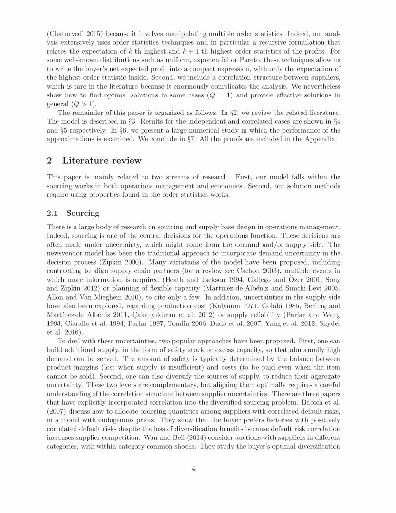
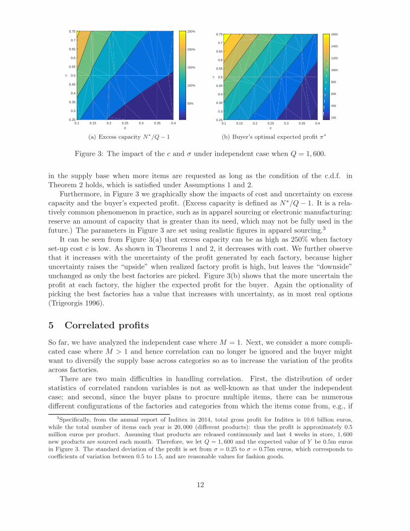
Furthermore, in Figure 3 we graphically show the impacts of cost and uncertainty on excesscapacity and the buyer’s expected profit. (Excess capacity is defined as N∗/Q− 1. It is a rela-tively common phenomenon in practice, such as in apparel sourcing or electronic manufacturing:reserve an amount of capacity that is greater than its need, which may not be fully used in thefuture.) The parameters in Figure 3 are set using realistic figures in apparel sourcing.3

It can be seen from Figure 3(a) that excess capacity can be as high as 250% when factoryset-up cost c is low. As shown in Theorems 1 and 2, it decreases with cost. We further observethat it increases with the uncertainty of the profit generated by each factory, because higheruncertainty raises the “upside” when realized factory profit is high, but leaves the “downside”unchanged as only the best factories are picked. Figure 3(b) shows that the more uncertain theprofit at each factory, the higher the expected profit for the buyer. Again the optionality ofpicking the best factories has a value that increases with uncertainty, as in most real options(Trigeorgis 1996).

5 Correlated profits

So far, we have analyzed the independent case where M = 1. Next, we consider a more compli-cated case where M > 1 and hence correlation can no longer be ignored and the buyer mightwant to diversify the supply base across categories so as to increase the variation of the profitsacross factories.

There are two main difficulties in handling correlation. First, the distribution of orderstatistics of correlated random variables is not as well-known as that under the independentcase; and second, since the buyer plans to procure multiple items, there can be numerousdifferent configurations of the factories and categories from which the items come from, e.g., if

3Specifically, from the annual report of Inditex in 2014, total gross profit for Inditex is 10.6 billion euros,while the total number of items each year is 20, 000 (different products): thus the profit is approximately 0.5million euros per product. Assuming that products are released continuously and last 4 weeks in store, 1, 600new products are sourced each month. Therefore, we let Q = 1, 600 and the expected value of Y be 0.5m eurosin Figure 3. The standard deviation of the profit is set from σ = 0.25 to σ = 0.75m euros, which corresponds tocoefficients of variation between 0.5 to 1.5, and are reasonable values for fashion goods.

12

Q = 2, the best items could be either both of them in category 1 or both in category 2, or oneof them in category 1 and the other in category 2.

5.1 Purchasing one item Q = 1

We start from the case where the buyer only requests one item. In this case, in every periodthe buyer only sources from one category, so we can avoid the second difficulty highlightedabove. Unlike that when the variables are i.i.d., where the c.d.f. of the highest order statistics

is HZ(1)(z) = G(z)∑M

m=1 Nm , the calculating of HZ(1) has to be decomposed into several steps.

Specifically, let Y(1)m denote the largest value among Ym1, · · · , YmNm , Z

(1)m = Xm+Y

(1)m , and Z(1)

be the largest one among all the items. Hence, HZ(1)(z) can be obtained through the followingthree steps:

1. Calculate the distribution of Y(1)m , which has c.d.f. G

Y(1)m

(z) = GNm ;

2. Calculate the distribution of Z(1)m , which has c.d.f. H

Z(1)m(z) =

∫∞

−∞f(x)G

Y(1)m

(z − x)dx;

3. Calculate the distribution of Z(1), which is HZ(1) =

M∏

m=1

HZ

(1)m

since the profits of the items

from different categories are independent.

By substituting HZ(1) and Q = 1 into (4), the buyer’s problem thereby can be rewritten as

maxN1,...,NM≥0

π(N1, . . . , NM ) =

∫ ∞

0

[

1−

M∏

m=1

∫ ∞

0f(x)G(z − x)Nmdx

]

dz −

M∑

m=1

cmNm, (11)

with the objective function being a nonlinear function defined on an integer vector space. Ingeneral, this is a very hard problem, because the usual convexity concept and the associatedKuhn-Tucker conditions do not apply. In this case, we are able to characterize some structuresin the optimal solution through concavity and submodularity (this is related to the concept ofL♮–convex in concrete analysis, first introduced by Murota (2003) and used by Lu and Song(2005), Zipkin (2008), Huh and Janakiraman (2010) or Chen et al. (2015) among others, as asubmodular set function can be identified with an L♮–convex function).

Lemma 2. Given M categories, the buyer’s expected net profit in (11):

(i) is concave with respect to each Nm, with the optimal number of factories in category mbeing given by the largest integer that satisfies

−

∫ ∞

0

M∏

m′=1,m′ 6=m

∫ ∞

0

f(x)G(z − x)Nm′dx

∫ ∞

0

f(x)G(z − x)Nm lnG(z − x)dx

dz ≥ cm; (12)

(ii) is submodular, i.e., π(Nm1 , N′

m2) − π(Nm1 , Nm2) decreases in Nm1 for all N

′

m2> Nm2 ,

m1,m2 = 1, · · · ,M and m1 6= m2.

Therefore, the first part of Lemma 2 is a direct extension of Theorem 2 with Q = 1, Xm = 0and there are other categories that compete with category m. From (12), we can tell that thespecific optimal number of factories in each category should depend on their specific variablecosts. Specifically, with the increase of cm, the optimal number of factories in each category N∗

m

13

should decrease, just like in the independent case. As to the second part of Lemma 2, it impliesthat the factories in different categories are substitutes. If the buyer cuts down the factories inone category, the number of factories in other categories will go up.

To obtain more insights of the original problem and investigate the impact of correlation,next we assume that the categories are symmetric, i.e., cm = c. In that case, from either (11) or(12), the optimal number of factories in each category N∗

m should be the same.4 The symmetricoptimal solution can be derived by solving

maxN≥0

π =

∫ ∞

0

{

1−

[∫ ∞

−∞

f(x)G(z − x)Ndx

]M}

dz − cMN. (13)

The optimal solution is uniquely determined by the integer below or above the solution to

−

∫ ∞

0

[∫ ∞

−∞

f(x)G(z − x)N∗

dx

]M−1 [∫ ∞

−∞

f(x)G(z − x)N∗

lnG(z − x)dx

]

dz = c. (14)

From (14), it can be seen that with the increase of c or M , N∗ will go down. Hence, themore categories there are, the less the factories in each category will be. That is, diversificationacross categories and factories per category are substitutes.

Further, to examine the impact of correlation, denote the correlation coefficient between theprofits of two items from the same category Zmjm = Xm + Ymjm and Zmj′m

= Xm + Ymj′mby ρ.

Therefore, given the variances ofXm and Ymjm being σ2X and σ2Y , we have ρ =σ2X

σ2X+σ2

Y

. In Table 2,

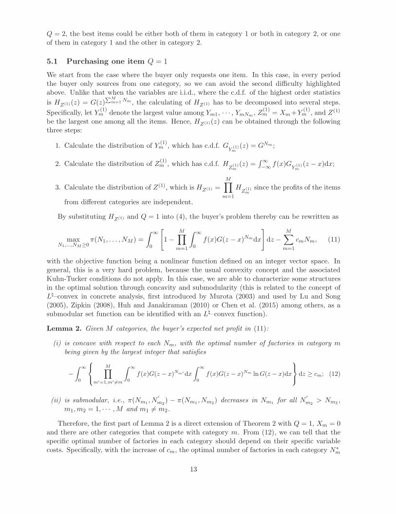
we examine the impacts of the correlation coefficient and uncertainty on the total optimalnumber of factories per category N∗ when there are two symmetric categories. Specifically, wesuppose the common part of the profit from each item X and the idiosyncratic term Y followUniform(a, b) and Uniform(c, d) respectively in the numerical example, with E[X +Y ] = µ =0.5 (million euros), just the same as that in Figure 3, although in this case we use Q = 1.5

From Table 2, it is interesting to see that the optimal number of factories under lowercorrelation coefficient is no less than that under higher correlation, in line with Chaturvedi andMartınez-de Albeniz (2016). Indeed, a higher correlation coefficient ρ implies that the impact ofthe uncertainty of common term X will be larger, and hence diversification with more factoriesper category is less effective: as a result, the number of factories is reduced. The variationwith respect to σ is in line with the findings for independent profits in §4: Table 2 once againdemonstrates that with the increase of uncertainty of the profit from each item, there will bemore factories, which is just the same as that under independent case in Figure 3(a). Specifically,it can be seen that excess capacity may be as high as eight times the needed quantity Q (seethe scenario ρ = 0.2 with σ = 0.75, where MN∗ = 8).

5.2 Purchasing multiple items Q > 1

When the buyer requests multiple items, similar to that in §5.1, an important step to analyze thebuyer’s decision (4) is to derive the distributions of the order statistics. Nevertheless, compared

4Given that this is a problem defined over integers, the optimal solution will be such that |N∗m1

−N∗m2

| ≤ 1.

5Let E[X+Y ] = µ and V ar(Z) = σ2, thena+ b

2+c+ d

2= µ,

(b− a)2

12= ρσ2 and

(d− c)2

12= (1−ρ)σ2. Thus,

it can be proved that b = a+2√

3ρσ2, c = µ−√

3ρσ2−√

3(1− ρ)σ2− a and d = µ−√

3ρσ2+√

3(1− ρ)σ2− a.Further, as in Figure 3, we discuss nine scenarios: σ = 0.25, 0.5 and 0.75, and ρ = 0.2, 0.5 and ρ = 0.8. Inaddition, without loss of generality, we set a = 0.3 (million euros) for all the numerical examples below and thesearch range is MN = 50.

14

Table 2: The impact of ρ and σ under correlated case when Q = 1 and M = 2.

σ = 0.25 a σ = 0.50 σ = 0.75c a N∗ π∗ a N∗ π∗ N∗ π∗

ρ = 0.2 0.10 a 2 0.42 3 0.57 4 0.830.15 1 0.35 2 0.45 3 0.660.20 1 0.30 2 0.35 2 0.520.25 1 0.25 2 0.25 2 0.420.30 1 0.20 1 0.20 2 0.320.35 1 0.15 1 0.15 2 0.220.40 1 0.10 1 0.10 1 0.13

ρ = 0.5 0.10 2 0.41 2 0.49 3 0.650.15 1 0.36 2 0.39 3 0.500.20 1 0.31 1 0.29 2 0.390.25 1 0.26 1 0.24 2 0.290.30 1 0.21 1 0.19 2 0.190.35 1 0.16 1 0.14 1 0.130.40 1 0.11 1 0.09 1 0.08

ρ = 0.8 0.10 1 0.41 2 0.43 3 0.470.15 1 0.36 1 0.36 2 0.370.20 1 0.31 1 0.31 1 0.280.25 1 0.26 1 0.26 1 0.230.30 1 0.21 1 0.21 1 0.180.35 1 0.16 1 0.16 1 0.130.40 1 0.11 1 0.11 1 0.08

a c, σ and π∗ in million euros.

to §5.1, we need k-th highest order statistics, instead of only the highest one. Analogously, thefirst step is to calculate the distribution of G

Y(k)m

, which can be derived from (6) and is GY

(k)m

(z) =

k∑

i=1

(

N

i− 1

)

G(z)N−i+1[1 − G(z)]i−1; the second step is to calculate the distribution of HZ

(k)m

,

i.e., the k-th highest profits among the suppliers from the same category, which is HZ

(k)m

(z) =∫ ∞

−∞

fXm(x)GY(k)m

(z−x)dx; and the last step is to calculate HZ(k), i.e., the distribution function

of k-th highest profit among all the suppliers regardless of their categories. Clearly. this processis computationally infeasible, especially for the third step since the items generating the first

k − 1 highest profits might come from any category and there are

(∑Mm=1Nm

k − 1

)

combinations

in total. Because obtaining exact analytical solution is not possible in general, we proceed asfollows. We first develop approximations that are easier to handle. Specifically, we derive oneupper bound and two lower bounds that provide effective solutions. We then solve the exactproblem numerically and test the quality of the approximations.

5.2.1 Upper bound

To look for the upper bound of the problem, let us revisit (1), i.e., the second stage problem,which is a linear program. We can convert this LP, referred to as the primal problem, into itsdual LP, by the strong duality theorem (Bertsimas and Tsitsiklis 1997). A feasible solution ofthe dual will provide an upper bound to the optimal value of the primal problem.

15

Suppose the dual variables for constraints∑Nm

jm=1 zmjm ≤ Nm,∑M

m=1

∑Nm

jm=1 zmjm ≤ Qand zmjm ≤ 1 are λm, µ and ηmjm , respectively, where m = 1, . . . ,M, and jm = 1, . . . , Nm.Therefore, the dual problem of (1) can be expressed as

minλm,µ,ηmjm

θ =

M∑

m=1

λmNm +

Nm∑

jm=1

ηmjm

+ µQ

s.t. λm + µ+ ηmjm ≥ Xm + Ymjm ,λm ≥ 0,µ ≥ 0,ηmjm ≥ 0, for m = 1, . . . ,M and jm = 1, . . . , Nm.

(15)

From strong duality, we know that the optimal value of (1) is no less than any feasible

solution of (15), i.e., R(

Q, {Xmt}, {Ymjmt})

≤ θ. As a result, the problem is to derive one

feasible solution that is easy to handle and at the same time is as close to the exact solution aspossible. And later by taking expectation and subtracting the cost

∑Mm=1 cmNm on both sides,

the upper bound of the original problem (2) can be derived. Hence, we first solve (15) and thenderive an upper bound of the original problem.

The dual LP (15) can be rewritten as a convex minimization problem as follows:

minλm,µ

θ =

M∑

m=1

λmNm +

Nm∑

jm=1

(Xm + Ymjm − λm − µ)+

+ µQ

s.t. λm ≥ 0,µ ≥ 0.

(16)

We can set λm = 0 to obtain a feasible solution and generate bounds for various values of µwhich takes the role of a parameter independent of the actual realizations of Xm, Ymjm . Weobtain the following upper bound for every realization of Xm, Ymjm :

R(

Q, {Xmt}, {Ymjmt})

≤ µQ+

M∑

m=1

Nm∑

jm=1

(Xm + Ymjm − µ)+. (17)

And then applying the expectation we obtain

π(N1, . . . , NM ) ≤µQ−

M∑

m=1

cmNm +

M∑

m=1

Nm∑

jm=1

E(Xm + Ymjm − µ)+

=µQ+

M∑

m=1

Nm

(∫ ∞

µ

Hm(z)dz − cm

)

,

(18)

where Hm(z) = 1−Hm(z) = 1−

∫ ∞

−∞

f(x)G(z − x)dx is the complementary c.d.f. of the profit

of each item in category m.Since as we mentioned in §3, the original problem is equivalent to a multi-object discrim-

inating auction with correlated valuations, we can also generate an upper bound by setting µfrom auction theory results. First, from Harris and Raviv (1981), we know that if all the bid-ders are risk-neutral and their valuations are independent, then a multi-object discriminatingauction will yield the same profit as that under a multi-object uniform-price auction, with the

16

price under uniform-price being the Q+1 highest profit. Second, note that for our problem, thecorrelation is mainly coming from Xm, the common term of the profits of the items sourced fromthe same category, and for different categories, the common term Xm may differ significantly.

Hence, considering these two points, we propose to use µ =

∑Mm=1NmXm∑M

m=1Nm

+E

[

Y (Q+1)m

]

, where

∑Mm=1NmXm∑M

m=1Nm

is the weighted average common term and E

[

Y (Q+1)m

]

is the expected profit of

the Q + 1 highest order statistic by only considering Ymjm . In particular, E[

Y (Q+1)m

]

can be

calculated by following the method illustrated in §4 and it is a function only with respect to Qand Nm since all the Ymjms are independent, m = 1, . . . ,M and jm = 1 . . . , Nm (specifically,

when the c.d.f. of Ymjm satisfies Assumption 1, then E

[

Y (Q+1)m

]

can be written as in Equation

7). In this case, a possible good upper bound with this approach is given by the right-hand side

of (18) with µ =

∑Mm=1NmXm∑M

m=1Nm

+ E

[

Y (Q+1)m

]

.

We can now maximize this upper bound with respect to N1, . . . , NM to obtain an upperbound to the optimal solution:

πU = maxN1,...,NM≥0

Qµ+

M∑

m=1

Nm

[∫ ∞

µ

Hm(z)dz − cm

]

s.t. µ =

∑Mm=1NmXm∑M

m=1Nm

+E

[

Y (Q+1)m

]

. (19)

5.2.2 Lower bounds

To study the lower bounds, we have to reformulate the buyer’s problem. The main idea is asfollows. First, it is worth noting that we can actually treat the problem of whether workingwith one factory, i.e., the decision of zmjm in the second stage, as an allocation problem. Thatis, suppose that the number of factories Nm in each category is given at the beginning of thesecond stage, and then the buyer decides how many items should be allocated to each category.Let qm denote the number of items allocated to category m, m = 1 · · ·M , which we again treatas a continuous variable. And then by backward induction, the optimal number of factories N∗

m

in each category can be derived after obtaining the optimal allocation q∗m. Formally, the buyer’sproblem can be written as max

N1,...,NM≥0EX,Y [π(N1, . . . , NM |X,Y )], where

π(N1, . . . , NM |X,Y ) = maxq1,...,qM≥0

J(X,Y, q) :=

M∑

m=1

qm∑

k=1

(Xm + Ymjm)(k)

−

M∑

m=1

cmNm

s.t. qm ≤ Nm, for m = 1, . . . ,M,M∑

m=1

qm ≤ Q.

(20)

We develop approximations from the perspective of stochastic programming. In our problem,the optimal value of qm in (20) depends on the realization of all Xm and Ymjm, m = 1, . . . ,M andjm = 1, . . . , Nm. From Theorem 1 in Avriel and Williams (1970), we know that EZ max

qJ(Z, q) ≥

maxq

EZJ(Z, q). As a result, the solution of the original is no less than a solution where qm is

independent of Ymjm and/or Xm. By exchanging the order in which the expectation and themaximum operators, we have

EX,Y [maxqJ(X,Y, q)] ≥ EX [max

qEY J(X,Y, q)] ≥ max

qEX,Y [J(X,Y, q)].

17

Therefore, we will use these two expected value solutions as two possible lower bounds, withthe first one involving π1(N1, . . . , NM |X) = max

q1,...,qM≥0EY J(X,Y, q), which requires solving the

maximization problem over q1, . . . , qM multiple times and may be complex in itself, and thesecond one involving π2(N1, . . . , NM ) = max

q1,...,qM≥0EX,Y J(X,Y, q), which looks the same as that

under independent case.

Lower bound 1. Given the value of Xm, the buyer only needs to consider the value of Ymjm

when making the allocation decision. That is,

π1(N1, . . . , NM |X) = maxq1,...,qM≥0

EY J(X,Y, q) =

M∑

m=1

(

qmXm +

qm∑

k=1

E

[

Y (k)m

]

)

−

M∑

m=1

cmNm

s.t. qm ≤ Nm, for m = 1, . . . ,M,M∑

m=1

qm ≤ Q.

(21)

Note that

qm∑

k=1

E

[

Y (k)m

]

in (21) is in fact the same as that sourcing Q items under indepen-

dent profits that has been discussed in §4, just replacing Q by qm. Therefore, given that the

distribution of Ymjm satisfies Assumption 1, i.e.,1−G(z)

g(z)= α+ βz, we have

qm∑

k=1

E

[

Y (k)m

]

= φ(qm)E[

Y (1)m

]

+ χ(qm) = φ(qm)ψ(Nm) + χ(qm).

As a result, the buyer’s expected profit under this situation is actually the expected profit of

π1(N1, . . . , NM |X) = maxq1,...,qM≥0

M∑

m=1

(qmXm + φ(qm)ψ(Nm) + χ(qm)− cmNm)

s.t. qm ≤ Nm, for m = 1, . . . ,M,M∑

m=1

qm ≤ Q,

(22)

which is a stochastic program for which optimality conditions can be characterized, as follows.

Letting ν be the the Lagrange multiplier for constraintM∑

m=1

qm ≤ Q, and ωm for that of qm ≤ Nm,

m = 1, . . . ,M , we obtain

Xm + φ′(qm)ψ(Nm) + χ′(qm) = ωm + ν.

This can be solved in closed form.6 Furthermore, by applying envelope theorem, the optimalnumber of factories that should be included into the supply base can be derived. That is, N∗

6For example, when G is uniform in [0, 1], it becomes:

Xm +2qm + 1

2ψ(Nm)−

2qm − 1

2= ωm + ν,

from Table 1 or equivalently

qm =1 + ψ(Nm)

2(1− ψ(Nm))+Xm − ωm − ν

(1− ψ(Nm)). (23)

Besides, complementarity slackness conditions means that ωm(Nm − qm) = 0, which means that at optimality, it

18

should satisfy

∂EXπ1(N1, . . . , NM |X)

∂Nm= EX [φ(q∗m)]ψ′(Nm) + EX [ω∗

m]− cm = 0,

where both ω∗m and q∗m depend on the realization of Xm and therefore are generally random

variables beforehand. Recall that under independent case, the optimal solution is ψ′(Nm) =cmφ(Q)

. The structure of the optimal solution under lower bound 1 is thus very similar, ψ′(Nm) =

cm − EX [ω∗m]

EX [φ(q∗m)]. The difference comes from the fact that, with multiple categories, the number of

factories used in category m is q∗m instead of Q, and the variable cost includes the availabilityshadow price c− ω∗

m, both of which depend on the realization of Xm.

Lower bound 2. We have

π2(N1, . . . , NM ) = maxq1,...,qM≥0

EX,Y J(X,Y, q) :=

M∑

m=1

qm∑

k=1

EX,Y

[

(Xm + Ymjm)(k)]

− cmNm

s.t. qm ≤ Nm, for m = 1, . . . ,M,M∑

m=1

qm ≤ Q,

(25)

which has the same structure as sourcing Q items under independent profits that has beendiscussed in §4. However, it differs from §4 in that the Zmjm = Xm+Ymjm, jm = 1, . . . , Nm, areall correlated for any m under this situation. Nevertheless, note that just like that under lowerbound 1, for the same category we have the same X, and thereby (Xm + Ymjm)

(k) = Xm+Y (k)m .

As a result, lower bound 2 can be rewritten as

π2(N1, . . . , NM ) = maxq1,...,qM≥0

EX,Y J(X,Y, q) :=

M∑

m=1

(qmE[Xm] + φ(qm)ψ(Nm) + χ(qm)− cmNm)

s.t. qm ≤ Nm, for m = 1, . . . ,M,M∑

m=1

qm ≤ Q,

(26)

with the optimal solution being derived by the same way as that under lower bound 1, which gives

φ′(qm)ψ(Nm)+χ′(qm)+E[Xm] = ωm+ν, ωm(Nm− qm) = 0 and ν

(

M∑

k=1

qm −Q

)

= 0.7 We can

depends whether ωm is below or over Xm +2qm + 1

2ψ(Nm)−

2qm − 1

2− ν, which results in

q∗m = min

{

Nm,1 + ψ(Nm)

2(1− ψ(Nm))+

Xm − ν

(1− ψ(Nm))

}

. (24)

Given this expression, we can find ν as the solution to

M∑

m=1

min

{

Nm,1 + ψ(Nm)

2(1− ψ(Nm))+

Xm − ν

(1− ψ(Nm))

}

= Q,

(or zero if there is no solution).7For instance, when G is uniform in [0, 1], we have

q∗m = min

{

Nm,1 + ψ(Nm)

2(1− ψ(Nm))+

E[Xm]− ν

(1− ψ(Nm))

}

, (27)

19

then maximize π2(N1, . . . , NM ) over N1, . . . , NM , which is now a standard stochastic programwith linear constraints, with the optimal solution being characterized as ψ′(Nm)φ(qm) = cm−ωm

by applying envelope theorem.

5.2.3 Summary of approximations

In summary, we have developed three tractable bounds for the original problem. Let πL2 andπL1 denote the optimal expected profit under lower bound 1 and lower bound 2, and thenthe relationship among the two lower bounds, the original problem and the upper bound aresummarized in Theorem 3.

Theorem 3. When the buyer sources multiple items, and there are M categories, πL2 ≤ πL1 ≤π∗ ≤ πU .

To evaluate the tightness of the bounds summarized in Theorem 3, we first discuss twoextreme cases, regarding the value of the correlation coefficient. Recall that it is defined as

ρ =σ2X

σ2X+σ2

Y

. As ρ approaches 1 (that is, the uncertainty of the category is the main risk), the

optimal solution under lower bound 1, i.e., πL1 approaches to the exact solution, i.e., π∗. Whenρ goes to 0, πL1 should goes to that of lower bound 2, i.e., πL2. Hence in that case, the qualityof lower bound 1 might be worse. Fortunately, in that scenario we can use §4 to determine theoptimal solution directly. As a result, our approximations provide a useful complement for ρ > 0to the solution approaches valid for ρ = 0.

6 Numerical study

To check the qualities of these approximations that we have illustrated above, a full comparisonamong the performances of these three heuristic solutions and the solution of the original problemis made, using an extensive Monte Carlo simulation. We first explore the symmetric case in §6.1,then discuss asymmetries over costs, within-category correlations and profit distributions in §6.2and finally provide extreme cases in which the approximated solutions perform less well in §6.3.

6.1 Symmetric case

We first suppose that there are only two symmetric categories and consider correlations ρ1 =ρ2 = 0.2, ρ1 = ρ2 = 0.5 and ρ1 = ρ2 = 0.8; and uncertainty σ1 = σ2 = 0.25, σ1 = σ2 = 0.5 andσ1 = σ2 = 0.75. We thus evaluate nine scenarios although we only report the four most extremecases in Table 3. We report optimal number of factories and expected profit, in comparison withthe exact optimal solution. Note that we find that the optimal number of suppliers under lowerbound 1 is almost always the same as that of the optimal solution, so we omit the results of thefactories changes under lower bound 1 in the table.

Several observations can be obtained from Table 3. First of all, the columns from the fifthto the sixth of Table 3 show the changes of the optimal number of factories under lower bound 2and that under upper bound, compared to that under the original problem. It can be seen thatwhen both the correlation coefficient ρ and the uncertainty of the profit σ are small, the optimal

and ν is the solution toM∑

m=1

min

{

Nm,1 + ψ(Nm)

2(1− ψ(Nm))+

E[Xm]− ν

(1− ψ(Nm))

}

= Q,

(or zero if there is no solution).

20

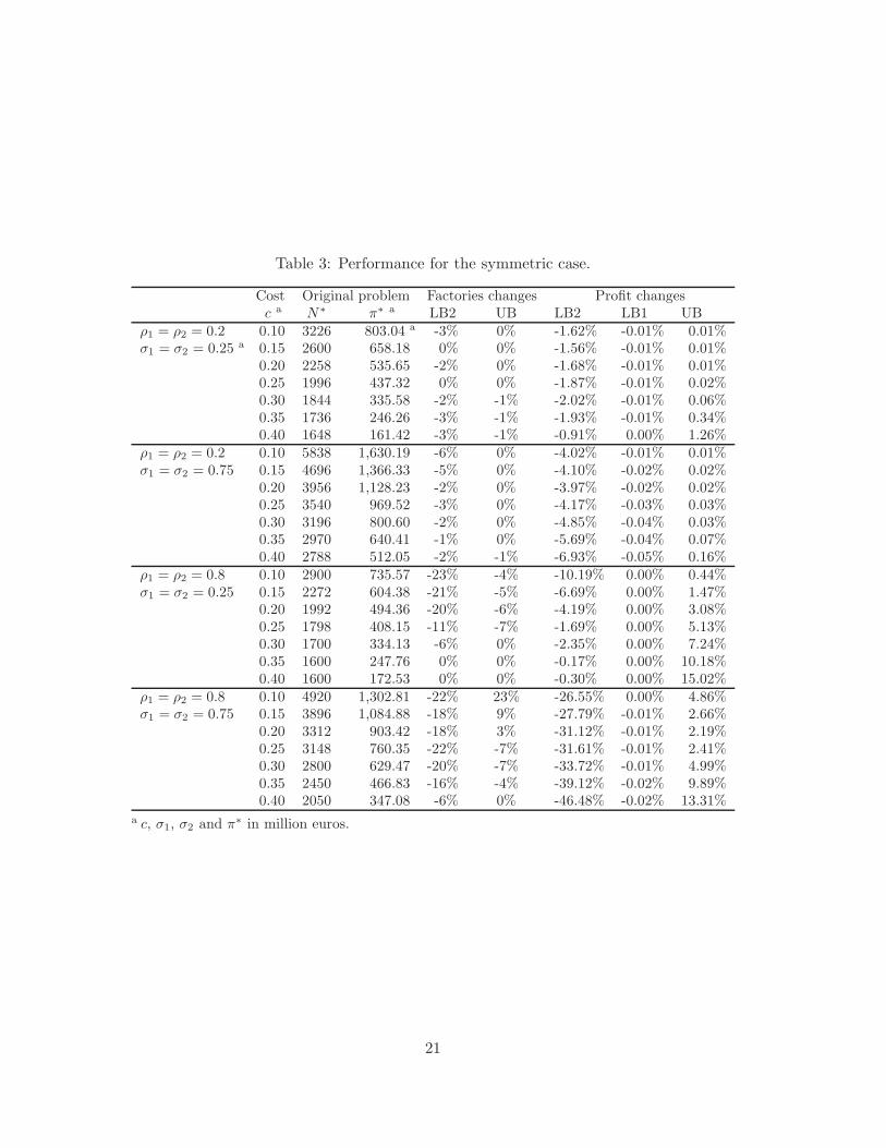
Table 3: Performance for the symmetric case.

Cost Original problem Factories changes Profit changesc a N∗ π∗ a LB2 UB LB2 LB1 UB

ρ1 = ρ2 = 0.2 0.10 3226 803.04 a -3% 0% -1.62% -0.01% 0.01%σ1 = σ2 = 0.25 a 0.15 2600 658.18 0% 0% -1.56% -0.01% 0.01%

0.20 2258 535.65 -2% 0% -1.68% -0.01% 0.01%0.25 1996 437.32 0% 0% -1.87% -0.01% 0.02%0.30 1844 335.58 -2% -1% -2.02% -0.01% 0.06%0.35 1736 246.26 -3% -1% -1.93% -0.01% 0.34%0.40 1648 161.42 -3% -1% -0.91% 0.00% 1.26%

ρ1 = ρ2 = 0.2 0.10 5838 1,630.19 -6% 0% -4.02% -0.01% 0.01%σ1 = σ2 = 0.75 0.15 4696 1,366.33 -5% 0% -4.10% -0.02% 0.02%

0.20 3956 1,128.23 -2% 0% -3.97% -0.02% 0.02%0.25 3540 969.52 -3% 0% -4.17% -0.03% 0.03%0.30 3196 800.60 -2% 0% -4.85% -0.04% 0.03%0.35 2970 640.41 -1% 0% -5.69% -0.04% 0.07%0.40 2788 512.05 -2% -1% -6.93% -0.05% 0.16%

ρ1 = ρ2 = 0.8 0.10 2900 735.57 -23% -4% -10.19% 0.00% 0.44%σ1 = σ2 = 0.25 0.15 2272 604.38 -21% -5% -6.69% 0.00% 1.47%

0.20 1992 494.36 -20% -6% -4.19% 0.00% 3.08%0.25 1798 408.15 -11% -7% -1.69% 0.00% 5.13%0.30 1700 334.13 -6% 0% -2.35% 0.00% 7.24%0.35 1600 247.76 0% 0% -0.17% 0.00% 10.18%0.40 1600 172.53 0% 0% -0.30% 0.00% 15.02%

ρ1 = ρ2 = 0.8 0.10 4920 1,302.81 -22% 23% -26.55% 0.00% 4.86%σ1 = σ2 = 0.75 0.15 3896 1,084.88 -18% 9% -27.79% -0.01% 2.66%

0.20 3312 903.42 -18% 3% -31.12% -0.01% 2.19%0.25 3148 760.35 -22% -7% -31.61% -0.01% 2.41%0.30 2800 629.47 -20% -7% -33.72% -0.01% 4.99%0.35 2450 466.83 -16% -4% -39.12% -0.02% 9.89%0.40 2050 347.08 -6% 0% -46.48% -0.02% 13.31%

a c, σ1, σ2 and π∗ in million euros.

21

number of factories derived by using these two approximations are relatively accurate. However,when either ρ or σ get large, the approximations are less accurate, which is especially significantwhen the cost is small. In contrast, the quality of lower bound 1 remains very high and thesuggested solution that maximizes πL1 is almost always the same as the optimal solution.

Second, the columns from the seventh to the ninth of Table 3 reveal the performance of theapproximations. It is apparent that lower bound 1 outstands among all these three heuristicsolutions, with the greatest discrepancy only being 0.05% (see the case ρ1 = ρ2 = 0.2, σ1 = σ2 =0.75, and c = 0.4), which implies that lower bound 1 is extremely accurate. The upper boundalso performs quite well, as long as the cost is not too expensive and the correlation coefficientof the profit is not too large. In particular, it is demonstrated that for most cases, the deviationof the upper bound is below 5%. But when the cost is high and the correlation is significant,the quality of the upper bound turns worse immediately, with the worst case being 15% (see thecase ρ1 = ρ2 = 0.8, σ1 = σ2 = 0.25, and c = 0.4). Further, the impact of σ on the performanceof upper bound is not monotonic, which depends on both the correlation coefficient and thecost. Take ρ1 = ρ2 = 0.8 for instance: with the increase of σ, the accuracy will go down whenthe cost is low, but then will go up when the cost gets larger. And when ρ1 and ρ2 change, therelationship between σ and the performance of the upper bound also changes. Finally, as to lowerbound 2, we can see that its performance is also very acceptable when both the correlation andthe uncertainty of the profit are not high (see the case ρ1 = ρ2 = 0.2, σ1 = σ2 = 0.25); whereaswith the increase of either the correlation coefficient ρ or the uncertainty of the profit σ, theperformance quality of lower bound 2 will get worse. This is especially true when ρ1 = ρ2 = 0.8,σ1 = σ2 = 0.75 and c = 0.4, with the profit difference percentage being as high as 46%.

In summary, we can highlight from this study on the symmetric case that the performanceof the heuristics tends to be very satisfactory and in particular lower bound 1 provides excellentsolutions for both the perspective of finding the optimal solution and providing a very tightlower bound on the actual optimal profit.

6.2 Asymmetric categories

We now turn to the asymmetric case. In particular, for the study of both the cost differencesand the correlation structure, we use σ1 = σ2 = 0.5 since as illustrated before the quality of theupper bound is not monotonic with respect to the uncertainty; and for the study of differentuncertainty level, the correlation coefficients are ρ1 = ρ2 = 0.8, which are parameters on whichthe performance of the heuristics is least good when categories are symmetric.

Cost differences. The optimal solution and the performances of the approximations whenthe costs of these two categories are asymmetric are presented in Table 4. Further, since whenρ1 = ρ2 = 0.2 and when ρ1 = ρ2 = 0.5, the performance of all these three approximations isquite good, with the largest deviation less than 0.2% and 5.5% respectively, we only report theresults when ρ1 = ρ2 = 0.8. From the third and fourth columns of Table 4 it can be seen thatthe buyer tends to allocate more factories to the category with cheaper cost, and the larger thegap between the costs, the larger the gap between the optimal number of factories in these twocategories. Besides this intuitive results, we observe that all the insights from §5.2 are preserved:overall performance is very satisfactory and lower bound 1 is always the best.

Correlation structure. Table 5 shows how the buyer should design the supply base whenthe intra-category correlation between these two categories is different. From Table 5, it canbe seen that it is better to source more items from the category in which the factories are less

22

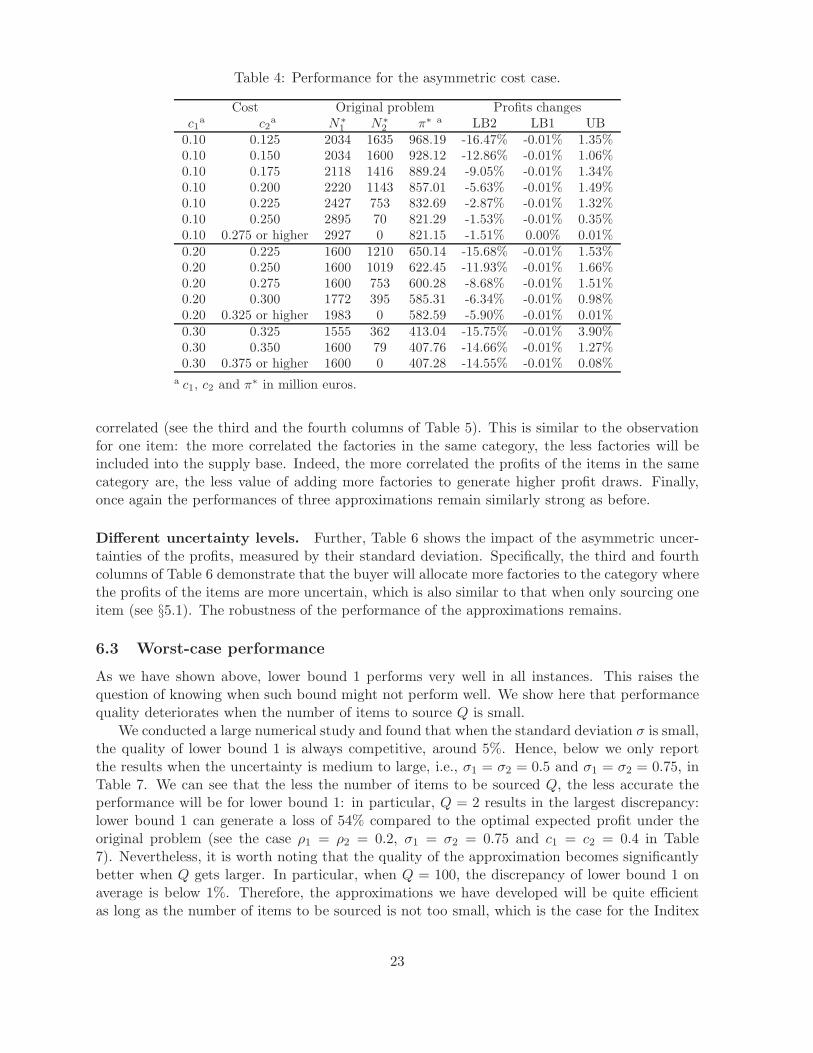
Table 4: Performance for the asymmetric cost case.

Cost Original problem Profits changesc1

a c2a N∗

1 N∗2 π∗ a LB2 LB1 UB

0.10 0.125 2034 1635 968.19 -16.47% -0.01% 1.35%0.10 0.150 2034 1600 928.12 -12.86% -0.01% 1.06%0.10 0.175 2118 1416 889.24 -9.05% -0.01% 1.34%0.10 0.200 2220 1143 857.01 -5.63% -0.01% 1.49%0.10 0.225 2427 753 832.69 -2.87% -0.01% 1.32%0.10 0.250 2895 70 821.29 -1.53% -0.01% 0.35%0.10 0.275 or higher 2927 0 821.15 -1.51% 0.00% 0.01%0.20 0.225 1600 1210 650.14 -15.68% -0.01% 1.53%0.20 0.250 1600 1019 622.45 -11.93% -0.01% 1.66%0.20 0.275 1600 753 600.28 -8.68% -0.01% 1.51%0.20 0.300 1772 395 585.31 -6.34% -0.01% 0.98%0.20 0.325 or higher 1983 0 582.59 -5.90% -0.01% 0.01%0.30 0.325 1555 362 413.04 -15.75% -0.01% 3.90%0.30 0.350 1600 79 407.76 -14.66% -0.01% 1.27%0.30 0.375 or higher 1600 0 407.28 -14.55% -0.01% 0.08%

a c1, c2 and π∗ in million euros.

correlated (see the third and the fourth columns of Table 5). This is similar to the observationfor one item: the more correlated the factories in the same category, the less factories will beincluded into the supply base. Indeed, the more correlated the profits of the items in the samecategory are, the less value of adding more factories to generate higher profit draws. Finally,once again the performances of three approximations remain similarly strong as before.

Different uncertainty levels. Further, Table 6 shows the impact of the asymmetric uncer-tainties of the profits, measured by their standard deviation. Specifically, the third and fourthcolumns of Table 6 demonstrate that the buyer will allocate more factories to the category wherethe profits of the items are more uncertain, which is also similar to that when only sourcing oneitem (see §5.1). The robustness of the performance of the approximations remains.

6.3 Worst-case performance

As we have shown above, lower bound 1 performs very well in all instances. This raises thequestion of knowing when such bound might not perform well. We show here that performancequality deteriorates when the number of items to source Q is small.

We conducted a large numerical study and found that when the standard deviation σ is small,the quality of lower bound 1 is always competitive, around 5%. Hence, below we only reportthe results when the uncertainty is medium to large, i.e., σ1 = σ2 = 0.5 and σ1 = σ2 = 0.75, inTable 7. We can see that the less the number of items to be sourced Q, the less accurate theperformance will be for lower bound 1: in particular, Q = 2 results in the largest discrepancy:lower bound 1 can generate a loss of 54% compared to the optimal expected profit under theoriginal problem (see the case ρ1 = ρ2 = 0.2, σ1 = σ2 = 0.75 and c1 = c2 = 0.4 in Table7). Nevertheless, it is worth noting that the quality of the approximation becomes significantlybetter when Q gets larger. In particular, when Q = 100, the discrepancy of lower bound 1 onaverage is below 1%. Therefore, the approximations we have developed will be quite efficientas long as the number of items to be sourced is not too small, which is the case for the Inditex

23

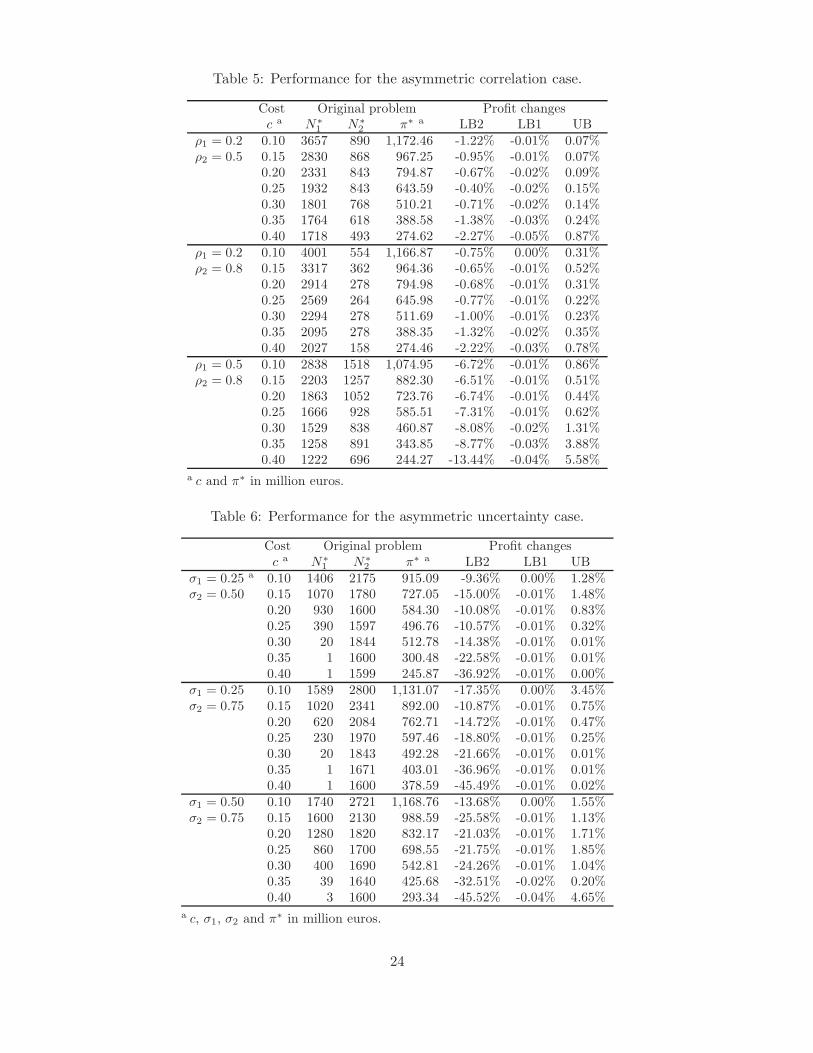
Table 5: Performance for the asymmetric correlation case.

Cost Original problem Profit changesc a N∗

1 N∗2 π∗ a LB2 LB1 UB

ρ1 = 0.2 0.10 3657 890 1,172.46 -1.22% -0.01% 0.07%ρ2 = 0.5 0.15 2830 868 967.25 -0.95% -0.01% 0.07%

0.20 2331 843 794.87 -0.67% -0.02% 0.09%0.25 1932 843 643.59 -0.40% -0.02% 0.15%0.30 1801 768 510.21 -0.71% -0.02% 0.14%0.35 1764 618 388.58 -1.38% -0.03% 0.24%0.40 1718 493 274.62 -2.27% -0.05% 0.87%

ρ1 = 0.2 0.10 4001 554 1,166.87 -0.75% 0.00% 0.31%ρ2 = 0.8 0.15 3317 362 964.36 -0.65% -0.01% 0.52%

0.20 2914 278 794.98 -0.68% -0.01% 0.31%0.25 2569 264 645.98 -0.77% -0.01% 0.22%0.30 2294 278 511.69 -1.00% -0.01% 0.23%0.35 2095 278 388.35 -1.32% -0.02% 0.35%0.40 2027 158 274.46 -2.22% -0.03% 0.78%

ρ1 = 0.5 0.10 2838 1518 1,074.95 -6.72% -0.01% 0.86%ρ2 = 0.8 0.15 2203 1257 882.30 -6.51% -0.01% 0.51%

0.20 1863 1052 723.76 -6.74% -0.01% 0.44%0.25 1666 928 585.51 -7.31% -0.01% 0.62%0.30 1529 838 460.87 -8.08% -0.02% 1.31%0.35 1258 891 343.85 -8.77% -0.03% 3.88%0.40 1222 696 244.27 -13.44% -0.04% 5.58%

a c and π∗ in million euros.

Table 6: Performance for the asymmetric uncertainty case.

Cost Original problem Profit changesc a N∗

1 N∗2 π∗ a LB2 LB1 UB

σ1 = 0.25 a 0.10 1406 2175 915.09 -9.36% 0.00% 1.28%σ2 = 0.50 0.15 1070 1780 727.05 -15.00% -0.01% 1.48%

0.20 930 1600 584.30 -10.08% -0.01% 0.83%0.25 390 1597 496.76 -10.57% -0.01% 0.32%0.30 20 1844 512.78 -14.38% -0.01% 0.01%0.35 1 1600 300.48 -22.58% -0.01% 0.01%0.40 1 1599 245.87 -36.92% -0.01% 0.00%

σ1 = 0.25 0.10 1589 2800 1,131.07 -17.35% 0.00% 3.45%σ2 = 0.75 0.15 1020 2341 892.00 -10.87% -0.01% 0.75%

0.20 620 2084 762.71 -14.72% -0.01% 0.47%0.25 230 1970 597.46 -18.80% -0.01% 0.25%0.30 20 1843 492.28 -21.66% -0.01% 0.01%0.35 1 1671 403.01 -36.96% -0.01% 0.01%0.40 1 1600 378.59 -45.49% -0.01% 0.02%

σ1 = 0.50 0.10 1740 2721 1,168.76 -13.68% 0.00% 1.55%σ2 = 0.75 0.15 1600 2130 988.59 -25.58% -0.01% 1.13%

0.20 1280 1820 832.17 -21.03% -0.01% 1.71%0.25 860 1700 698.55 -21.75% -0.01% 1.85%0.30 400 1690 542.81 -24.26% -0.01% 1.04%0.35 39 1640 425.68 -32.51% -0.02% 0.20%0.40 3 1600 293.34 -45.52% -0.04% 4.65%

a c, σ1, σ2 and π∗ in million euros.

24

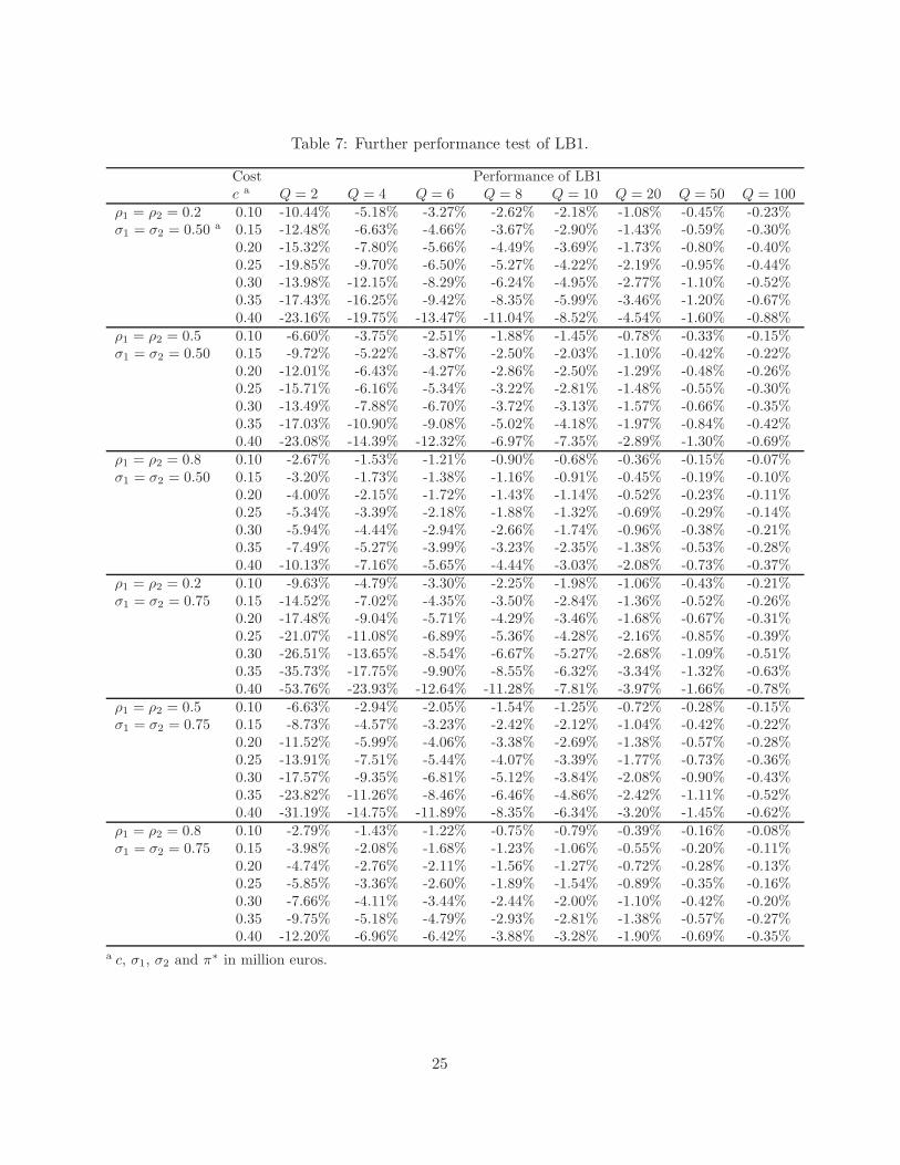
Table 7: Further performance test of LB1.

Cost Performance of LB1c a Q = 2 Q = 4 Q = 6 Q = 8 Q = 10 Q = 20 Q = 50 Q = 100

ρ1 = ρ2 = 0.2 0.10 -10.44% -5.18% -3.27% -2.62% -2.18% -1.08% -0.45% -0.23%σ1 = σ2 = 0.50 a 0.15 -12.48% -6.63% -4.66% -3.67% -2.90% -1.43% -0.59% -0.30%

0.20 -15.32% -7.80% -5.66% -4.49% -3.69% -1.73% -0.80% -0.40%0.25 -19.85% -9.70% -6.50% -5.27% -4.22% -2.19% -0.95% -0.44%0.30 -13.98% -12.15% -8.29% -6.24% -4.95% -2.77% -1.10% -0.52%0.35 -17.43% -16.25% -9.42% -8.35% -5.99% -3.46% -1.20% -0.67%0.40 -23.16% -19.75% -13.47% -11.04% -8.52% -4.54% -1.60% -0.88%

ρ1 = ρ2 = 0.5 0.10 -6.60% -3.75% -2.51% -1.88% -1.45% -0.78% -0.33% -0.15%σ1 = σ2 = 0.50 0.15 -9.72% -5.22% -3.87% -2.50% -2.03% -1.10% -0.42% -0.22%

0.20 -12.01% -6.43% -4.27% -2.86% -2.50% -1.29% -0.48% -0.26%0.25 -15.71% -6.16% -5.34% -3.22% -2.81% -1.48% -0.55% -0.30%0.30 -13.49% -7.88% -6.70% -3.72% -3.13% -1.57% -0.66% -0.35%0.35 -17.03% -10.90% -9.08% -5.02% -4.18% -1.97% -0.84% -0.42%0.40 -23.08% -14.39% -12.32% -6.97% -7.35% -2.89% -1.30% -0.69%

ρ1 = ρ2 = 0.8 0.10 -2.67% -1.53% -1.21% -0.90% -0.68% -0.36% -0.15% -0.07%σ1 = σ2 = 0.50 0.15 -3.20% -1.73% -1.38% -1.16% -0.91% -0.45% -0.19% -0.10%

0.20 -4.00% -2.15% -1.72% -1.43% -1.14% -0.52% -0.23% -0.11%0.25 -5.34% -3.39% -2.18% -1.88% -1.32% -0.69% -0.29% -0.14%0.30 -5.94% -4.44% -2.94% -2.66% -1.74% -0.96% -0.38% -0.21%0.35 -7.49% -5.27% -3.99% -3.23% -2.35% -1.38% -0.53% -0.28%0.40 -10.13% -7.16% -5.65% -4.44% -3.03% -2.08% -0.73% -0.37%

ρ1 = ρ2 = 0.2 0.10 -9.63% -4.79% -3.30% -2.25% -1.98% -1.06% -0.43% -0.21%σ1 = σ2 = 0.75 0.15 -14.52% -7.02% -4.35% -3.50% -2.84% -1.36% -0.52% -0.26%

0.20 -17.48% -9.04% -5.71% -4.29% -3.46% -1.68% -0.67% -0.31%0.25 -21.07% -11.08% -6.89% -5.36% -4.28% -2.16% -0.85% -0.39%0.30 -26.51% -13.65% -8.54% -6.67% -5.27% -2.68% -1.09% -0.51%0.35 -35.73% -17.75% -9.90% -8.55% -6.32% -3.34% -1.32% -0.63%0.40 -53.76% -23.93% -12.64% -11.28% -7.81% -3.97% -1.66% -0.78%

ρ1 = ρ2 = 0.5 0.10 -6.63% -2.94% -2.05% -1.54% -1.25% -0.72% -0.28% -0.15%σ1 = σ2 = 0.75 0.15 -8.73% -4.57% -3.23% -2.42% -2.12% -1.04% -0.42% -0.22%

0.20 -11.52% -5.99% -4.06% -3.38% -2.69% -1.38% -0.57% -0.28%0.25 -13.91% -7.51% -5.44% -4.07% -3.39% -1.77% -0.73% -0.36%0.30 -17.57% -9.35% -6.81% -5.12% -3.84% -2.08% -0.90% -0.43%0.35 -23.82% -11.26% -8.46% -6.46% -4.86% -2.42% -1.11% -0.52%0.40 -31.19% -14.75% -11.89% -8.35% -6.34% -3.20% -1.45% -0.62%

ρ1 = ρ2 = 0.8 0.10 -2.79% -1.43% -1.22% -0.75% -0.79% -0.39% -0.16% -0.08%σ1 = σ2 = 0.75 0.15 -3.98% -2.08% -1.68% -1.23% -1.06% -0.55% -0.20% -0.11%

0.20 -4.74% -2.76% -2.11% -1.56% -1.27% -0.72% -0.28% -0.13%0.25 -5.85% -3.36% -2.60% -1.89% -1.54% -0.89% -0.35% -0.16%0.30 -7.66% -4.11% -3.44% -2.44% -2.00% -1.10% -0.42% -0.20%0.35 -9.75% -5.18% -4.79% -2.93% -2.81% -1.38% -0.57% -0.27%0.40 -12.20% -6.96% -6.42% -3.88% -3.28% -1.90% -0.69% -0.35%

a c, σ1, σ2 and π∗ in million euros.

25

example described in the introduction.Note finally that the worst-case performance is always achieved when Q = 1. It turns out

that this case can be solved optimally, as shown in §5.1, which means that we can use an exactalgorithm to find the best solution. Hence, our analysis provides two solution approaches (exactand approximated), so that in all cases one of them will perform well.

7 Concluding remarks

Supply base design is a particularly important and challenging decision for a buyer of innovativeproducts. In this paper, we have developed a tractable framework for this type of decisions.Given a fixed number of categories, we optimize the number of suppliers that the the buyershould include into the supply base, taking into account the potential profitability of the (risky)design offered by each supplier. To do that, we manipulate high order statistics with or withoutcorrelation within a category. We derive structural results and closed form solutions whensupplier profitabilities are independent or when they are correlated but with a single winner.In contrast, exact solutions are not available in the general correlated case, so we developapproximations which provide near-optimal solutions. Besides the methodological achievements,we also provide insights which may be valuable to the buyer. We find that uncertainty isbeneficial for the buyer and leads to bigger supply bases. In particular, higher correlation isworse for the system because it induces less variability across suppliers.

Our model also reveals some limitations: for simplicity, we assumed that the supply base isfixed during the planning horizon and only allocation to suppliers varies over time. In reality,supply base management is a continuous process where each year, some suppliers are lost andnew suppliers are qualified (Chaturvedi et al. 2014). Future research should provide a closerlook at these dynamics. For instance, supplier scorecards are periodically updated and it wouldbe interesting to see how the joint decision regarding business allocations and supply basemaintenance should depend on it. The type of relationship with suppliers should also be governedmore carefully: it is likely that longer relationships have beneficial effects on investment andquality, so perhaps narrower supply bases might be optimal when incentives come into play (Liand Debo 2009, Aoki and Lennerfors 2013).

26

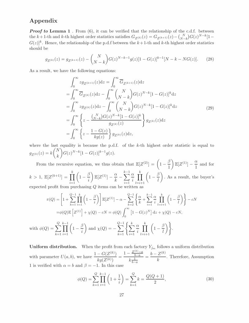
Appendix

Proof to Lemma 1 . From (6), it can be verified that the relationship of the c.d.f. betweenthe k+1-th and k-th highest order statistics satisfies GZ(k)(z) = GZ(k+1)(z)−

(

NN−k

)

G(z)N−k[1−

G(z)]k. Hence, the relationship of the p.d.f between the k+1-th and k-th highest order statisticsshould be

gZ(k)(z) = gZ(k+1)(z) −

(

N

N − k

)

G(z)N−k−1g(z)[1 −G(z)]k−1[N − k −NG(z)]. (28)

As a result, we have the following equations:∫ ∞

0zgZ(k+1)(z)dz =

∫ ∞

0GZ(k+1)(z)dz

=

∫ ∞

0GZ(k)(z)dz −

∫ ∞

0

(

N

N − k

)

G(z)N−k[1−G(z)]kdz

=

∫ ∞

0zgZ(k)(z)dz −

∫ ∞

0

(

N

N − k

)

G(z)N−k[1−G(z)]kdz

=

∫ ∞

0

{

z −

(

NN−k

)

G(z)N−k[1−G(z)]k

gZ(k)(z)

}

gZ(k)(z)dz

=

∫ ∞

0

{

z −1−G(z)

kg(z)

}

gZ(k)(z)dz,

(29)

where the last equality is because the p.d.f. of the k-th highest order statistic is equal to

gZ(k)(z) = k

(

N

k

)

G(z)N−k[1−G(z)]k−1g(z).

From the recursive equation, we thus obtain that E[Z(2)] =

(

1−β

1

)

E[Z(1)] −α

1and for

k > 1, E[Z(k+1)] =k∏

i=1

(

1−β

i

)

E[Z(1)] −α

k−

k−1∑

i=1

α

i

k∏

l=i+1

(

1−β

l

)

. As a result, the buyer’s

expected profit from purchasing Q items can be written as

π(Q) =

[

1 +

Q−1∑

k=1

k∏

i=1

(

1−β

i

)

]

E[Z(1)]− α−

Q−1∑

k=2

{

α

k+

k−1∑

i=1

α

i

k∏

l=i+1

(

1−β

l

)

}

− cN

=φ(Q)E[

Z(1)]

+ χ(Q)− cN = φ(Q)

∫ ∞

0

[

1−G(z)N]

dz + χ(Q)− cN,

with φ(Q) =

Q∑

k=1

k−1∏

i=1

(

1−β

i

)

and χ(Q) = −

Q−1∑

k=1

{

k∑

i=1

α

i

k∏

l=i+1

(

1−β

l

)

}

.

Uniform distribution. When the profit from each factory Yjm follows a uniform distribution

with parameter U(a, b), we have1−G(Z(k))

kg(Z(k))=

1− Z(k)−ab−a

k 1b−a

=b− Z(k)

k. Therefore, Assumption

1 is verified with α = b and β = −1. In this case

φ(Q) =

Q∑

k=1

k−1∏

i=1

(

1 +1

i

)

=

Q∑

k=1

k =Q(Q+ 1)

2, (30)

27

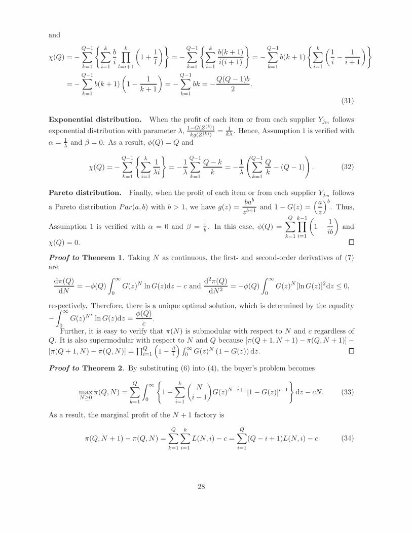
and

χ(Q) =−

Q−1∑

k=1

{

k∑

i=1

b

i

k∏

l=i+1

(

1 +1

l

)

}

= −

Q−1∑

k=1

{

k∑

i=1

b(k + 1)

i(i+ 1)

}

= −

Q−1∑

k=1

b(k + 1)

{

k∑

i=1

(

1

i−

1

i+ 1

)

}

=−

Q−1∑

k=1

b(k + 1)

(

1−1

k + 1

)

= −

Q−1∑

k=1

bk = −Q(Q− 1)b

2.

(31)

Exponential distribution. When the profit of each item or from each supplier Yjm follows

exponential distribution with parameter λ, 1−G(Z(k))

kg(Z(k))= 1

kλ . Hence, Assumption 1 is verified with

α = 1λand β = 0. As a result, φ(Q) = Q and

χ(Q) =−

Q−1∑

k=1

{

k∑

i=1

1

λi

}

= −1

λ

Q−1∑

k=1

Q− k

k= −

1

λ

(

Q−1∑

k=1

Q

k− (Q− 1)

)

. (32)

Pareto distribution. Finally, when the profit of each item or from each supplier Yjm follows

a Pareto distribution Par(a, b) with b > 1, we have g(z) =bab

zb+1and 1 − G(z) =

(a

z

)b

. Thus,

Assumption 1 is verified with α = 0 and β = 1b. In this case, φ(Q) =

Q∑

k=1

k−1∏

i=1

(

1−1

ib

)

and

χ(Q) = 0.

Proof to Theorem 1. Taking N as continuous, the first- and second-order derivatives of (7)are

dπ(Q)

dN= −φ(Q)

∫ ∞

0G(z)N lnG(z)dz − c and

d2π(Q)

dN2= −φ(Q)

∫ ∞

0G(z)N [lnG(z)]2dz ≤ 0,

respectively. Therefore, there is a unique optimal solution, which is determined by the equality

−

∫ ∞

0G(z)N

∗

lnG(z)dz =φ(Q)

c.

Further, it is easy to verify that π(N) is submodular with respect to N and c regardless ofQ. It is also supermodular with respect to N and Q because [π(Q+ 1, N + 1)− π(Q,N + 1)]−

[π(Q+ 1, N)− π(Q,N)] =∏Q

i=1

(

1− βi

)

∫∞

0 G(z)N (1−G(z)) dz.

Proof to Theorem 2. By substituting (6) into (4), the buyer’s problem becomes

maxN≥0

π(Q,N) =

Q∑

k=1

∫ ∞

0

{

1−k∑

i=1

(

N

i− 1

)

G(z)N−i+1[1−G(z)]i−1

}

dz − cN. (33)

As a result, the marginal profit of the N + 1 factory is

π(Q,N + 1)− π(Q,N) =

Q∑

k=1

k∑

i=1

L(N, i)− c =

Q∑

i=1

(Q− i+ 1)L(N, i) − c (34)

28

with L(N, i) =

∫ ∞

0G(z)N+1−i[1−G(z)]i−1

(

N

i− 1

){

1−N + 1

N − i+ 2G(z)

}

dz. This yields

π(Q+ 1, N + 1)− π(Q+ 1, N) =

Q+1∑

i=1

(Q+ 1− i+ 1)L(N, i) − c

=

Q∑

i=1

(Q− i+ 1)L(N, i) +

Q+1∑

i=1

L(N, i)− c = π(Q,N + 1)− π(Q,N) +

Q+1∑

i=1

L(N, i).

(35)

Consequently, the buyer’s expected profit π(Q,N) is supermodular with respect to N and Q

when L(N, i) =

∫ ∞

0G(z)N+1−i[1−G(z)]i−1

(

N

i− 1

){

1−N + 1

N − i+ 2G(z)

}

dz ≥ 0.

Further, note that

L(N, i)− L(N − 1, i)

=

(

N − 1

i− 1

)∫ ∞

0

G(z)N−i[1−G(z)]i−1

{

−N(N + 1)

(N − i+ 1)(N − i + 2)G2(z) +

2N

N − i+ 1G(z)− 1

}

dz

≤

(

N − 1

i− 1

)∫ ∞

0

G(z)N−i[1−G(z)]i−1

{

−(N + 1)2

(N − i+ 2)2G2(z) +

2N

N − i+ 1G(z)− 1

}

dz

≤

(

N − 1

i− 1

)∫ ∞

0

G(z)N−i[1−G(z)]i−1

{

2N

N − i+ 1G(z)−

4(N + 1)

N − i+ 2G(z)

}

dz

=2

(

N − 1

i− 1

)∫ ∞

0

G(z)N+1−i[1−G(z)]i−1 −(N + 2)(N − i)− 2

(N − i+ 1)(N − i+ 2)dz ≤ 0,

where the first inequality is due toN

N − i+ 1≤

N + 1

N − i+ 2, the second inequality is due to

−a2− b2 ≤ −4ab with a = (N +1)/(N − i+2)G(z) and b = 1, and the third equality is becausei is always no greater than N . As a result, the buyer’s expected profit function is unimodal and

there is a unique solution, which is the largest integer that satisfies

Q∑

i=1

(Q−i+1)L(N, i) ≥ c.

Proof to Lemma 2. We first calculate the first-order difference of the profit with respect toNm, in the category where Nm > 0:

π(Nm + 1)− π(Nm)

=

∫ ∞

0

∫ ∞

−∞

f(x)G(z − x)Nm(1−G(z − x))dxM∏

m′=1,m′ 6=m

∫ ∞

−∞

f(x)G(z − x)Nm′dx

dz − cm.

Since G(z − x) ≤ 1, this is decreasing in Nm so π is concave in Nm, which proves part (i).Similarly, this is decreasing in Nm1 for any m1 6= m, which proves submodularity, i.e., part (ii).

When the categories are symmetric, first, from the KKT conditions we can derive the can-didate of the optimal solution, which satisfies

∂πb∂N

= −

∫ ∞

0MH

Z(1)m

(z)M−1dH

Z(1)m(z)

dNdz − cM = 0. (36)

29

To check out whether this one should be the best, next the second order derivative is derived,which is:

∂2πb∂N2

= −

∫ ∞

0

M(M − 1)HZ

(1)m

(z)M−2

(

dHZ

(1)m

(z)

dN

)2

+MHZ

(1)m

(z)M−1d2H

Z(1)m

(z)

dN2

dz, (37)

whereHZ

(1)m

(z) =∫∞

−∞fXi

(x)GY (z−x)Ndx,

dHZ

(1)m(z)

dN=

∫ ∞

−∞

fX(x)GY (z−x)N ln[GY (z−x)]dx

andd2H

Z(1)m(z)

dN2=

∫ ∞

−∞

fX(x)GY (z − x)N {ln[GY (l − x)]}2 dx ≥ 0. As a result,

∂2πb∂N2

=−

∫ ∞

0

M(M − 1)HZ

(1)m

(z)M−2

(

dHZ

(1)m

(z)

dN

)2

+M [HZ

(1)m

(z)]M−1d2H

Z(1)m

(z)

dN2

dz ≤ 0.

References

Allon, G., and J. A. Van Mieghem. 2010. Global dual sourcing: Tailored base-surge allocation to near-andoffshore production. Management Science 56 (1): 110–124.

Aoki, K., and T. T. Lennerfors. 2013. The New, Improved Keiretsu. Harvard Business Review 91 (9):109.

Arellano-Valle, R. B., and M. G. Genton. 2007. On the exact distribution of linear combinations of orderstatistics from dependent random variables. Journal of Multivariate Analysis 98 (10): 1876–1894.

Avriel, M., and A. Williams. 1970. The value of information and stochastic programming. OperationsResearch 18 (5): 947–954.

Babich, V., A. N. Burnetas, and P. H. Ritchken. 2007. Competition and diversification effects in supplychains with supplier default risk. Manufacturing & Service Operations Management 9 (2): 123–146.

Berling, P., and V. Martınez-de Albeniz. 2011. Optimal inventory policies when purchase price anddemand are stochastic. Operations Research 59 (1): 109–124.

Bertsimas, D., and J. N. Tsitsiklis. 1997. Introduction to linear optimization, Volume 6. Athena ScientificBelmont, MA.

Cachon, G. P. 2003. Supply chain coordination with contracts. Handbooks in Operations Research andManagement Science 11:227–339.

Cakanyıldırım, M., Q. Feng, X. Gan, and S. P. Sethi. 2012. Contracting and coordination under asym-metric production cost information. Production and Operations Management 21 (2): 345–360.

Caro, F., and V. Martınez-de Albeniz. 2015. Fast fashion: Business model overview and research op-portunities. In Retail Supply Chain Management: Quantitative Models and Empirical Studies, 2ndEdition, ed. N. Agrawal and S. A. Smith, 237–264. Springer, New York.

Chaturvedi, A. 2015. Procurement auctions with capacity constrained suppliers. European Journal ofOperational Research 247 (3): 987–995.

Chaturvedi, A., D. R. Beil, and V. Martınez-de-Albeniz. 2014. Split-award auctions for supplier retention.Management Science 60 (7): 1719–1737.

Chaturvedi, A., and V. Martınez-de Albeniz. 2016. Safety Stock, Excess Capacity or Diversification:Trade-Offs under Supply and Demand Uncertainty. Production and Operations Management 25(1): 77–95.

Chen, X., X. Gao, and Z. Hu. 2015. A new approach to two-location joint inventory and transshipmentcontrol via L-convexity. Operations Research Letters 43 (1): 65–68.

30

Choi, T. Y., and D. R. Krause. 2006. The supply base and its complexity: Implications for transactioncosts, risks, responsiveness, and innovation. Journal of Operations Management 24 (5): 637–652.

Ciarallo, F., R. Akella, and T. Morton. 1994. A periodic review, production planning model with uncertaincapacity and uncertain demand-optimality of extended myopic policies. Management Science 40(3): 320–332.

Dada, M., N. Petruzzi, and L. Schwarz. 2007. A Newsvendors procurement problem with unreliablesuppliers. Manufacturing & Service Operations Management 9 (1): 9–32.

David, H. A., and H. Nagaraja. 2003. Order statistics . Third Edition ed. Wiley series in probability andstatistics. Wiley, New York.

Diamond, J. 2017. Trump floats 20 percent tax on Mexican imports to pay for wall, but considering otheroptions. CNN January 27:online.

Fisher, M. L. 1997. What is the right supply chain for your product? Harvard Business Review 75:105–117.

Gallego, G., and O. Ozer. 2001. Integrating replenishment decisions with advance demand information.Management Science 47 (10): 1344–1360.

Golabi, K. 1985. Optimal inventory policies when ordering prices are random. Operations Research 33(3): 575–588.

Harris, M., and A. Raviv. 1981. Allocation mechanisms and the design of auctions. Econometrica:Journal of the Econometric Society 49 (6): 1477–1499.

Heath, D. C., and P. L. Jackson. 1994. Modeling the Evolution of Demand Forecasts with Applicationto Safety Stock Analysis in Production/Distribution Systems. IIE Transactions 26 (3): 17–30.

Hill, W. G. 1976. Order statistics of correlated variables and implications in genetic selection programmes.Biometrics 32 (4): 889–902.

Hua, K. 2016. Pre-Fall Collections 2017: Fashion Trends to Look for This Year. Forbes December16:online.

Huh, W. T., and G. Janakiraman. 2010. On the optimal policy structure in serial inventory systems withlost sales. Operations Research 58 (2): 486–491.

Inditex 2015. Annual report.

Jamalizadeh, A., and N. Balakrishnan. 2010. Distributions of order statistics and linear combinationsof order statistics from an elliptical distribution as mixtures of unified skew-elliptical distributions.Journal of Multivariate Analysis 101 (6): 1412–1427.

Kalymon, B. A. 1971. Stochastic prices in a single-item inventory purchasing model. Operations Re-search 19 (6): 1434–1458.

Li, C., and L. Debo. 2009. Second Sourcing vs. Sole Sourcing with Capacity Investment and AsymmetricInformation. Manufacturing & Service Operations Management 11 (3): 448–470.

Lu, Y., and J.-S. Song. 2005. Order-based cost optimization in assemble-to-order systems. OperationsResearch 53 (1): 151–169.

Martınez-de-Albeniz, V., and D. Simchi-Levi. 2005. A portfolio approach to procurement contracts.Production and Operations Management 14 (1): 90–114.

Milgrom, P. R., and R. J. Weber. 1982. A theory of auctions and competitive bidding. Econometrica:Journal of the Econometric Society 50 (5): 1089–1122.

Murota, K. 2003. Discrete convex analysis. SIAM.

Myerson, R. B. 1981. Optimal auction design. Mathematics of Operations Research 6 (1): 58–73.

Owen, D. B., G. P. Steck et al. 1962. Moments of order statistics from the equicorrelated multivariatenormal distribution. The Annals of Mathematical Statistics 33 (4): 1286–1291.

Parlar, M. 1997. An inventory problem with two randomly available suppliers. Operations Research 45(6): 904–918.

Parlar, M., and D. Wang. 1993. Diversification under yield randomness in inventory models. EuropeanJournal of Operational Research 66 (1): 52–64.

31

Rawlings, J. 1976. Order statistics for a special class of unequally correlated multinormal variates.Biometrics 32 (4): 875–887.

Snyder, L. V., Z. Atan, P. Peng, Y. Rong, A. J. Schmitt, and B. Sinsoysal. 2016. OR/MS models forsupply chain disruptions: A review. IIE Transactions 48 (2): 89–109.

Song, J.-S., and P. H. Zipkin. 2012. Newsvendor problems with sequentially revealed demand information.Naval Research Logistics (NRL) 59 (8): 601–612.

Tokatli, N. 2008. Global sourcing: insights from the global clothing industrythe case of Zara, a fastfashion retailer. Journal of Economic Geography 8 (1): 21–38.

Tomlin, B. 2006. On the value of mitigation and contingency strategies for managing supply chaindisruption risks. Management Science 52 (5): 639.

Trigeorgis, L. 1996. Real options: Managerial flexibility and strategy in resource allocation. MIT press,Cambridge MA.

Vickrey, W. 1961. Counterspeculation, auctions, and competitive sealed tenders. The Journal of Fi-nance 16 (1): 8–37.

Wan, Z., and D. R. Beil. 2009. RFQ auctions with supplier qualification screening. Operations Research 57(4): 934–949.

Wan, Z., and D. R. Beil. 2014. Bid-taker power and supply base diversification. Manufacturing & ServiceOperations Management 16 (2): 300–314.

Wiens, D. P., N. C. Beaulieu, and P. Loskot. 2006. On the exact distribution of the sum of the largest n-k out of n normal random variables with differing mean values. Statistics 40 (2): 165–173.

Yang, Z., G. Aydın, V. Babich, and D. R. Beil. 2012. Using a dual-sourcing option in the presence ofasymmetric information about supplier reliability: Competition vs. diversification. Manufacturing& Service Operations Management 14 (2): 202–217.

Zipkin, P. 2000. Foundations of inventory management. Irwin/McGraw-Hill, Boston MA.

Zipkin, P. 2008. On the structure of lost-sales inventory models. Operations Research 56 (4): 937–944.

32