support vector machines - carnegie mellon school of...
TRANSCRIPT
Machine Learning
10-701, Fall 2015
Support Vector Machines
Eric Xing
Lecture 9, October 8, 2015
1
Reading: Chap. 6&7, C.B book, and listed papers© Eric Xing @ CMU, 2006-2015

2
What is a good Decision Boundary? Consider a binary classification
task with y = ±1 labels (not 0/1 as before).
When the training examples are linearly separable, we can set the parameters of a linear classifier so that all the training examples are classified correctly
Many decision boundaries! Generative classifiers Logistic regressions …
Are all decision boundaries equally good?
Class 1
Class 2
© Eric Xing @ CMU, 2006-2015

3
Not All Decision Boundaries Are Equal!
Why we may have such boundaries? Irregular distribution Imbalanced training sizes outliners
© Eric Xing @ CMU, 2006-2015

4
Classification and Margin Parameterzing decision boundary
Let w denote a vector orthogonal to the decision boundary, and b denote a scalar "offset" term, then we can write the decision boundary as:
0TT
T
wbx
ww
Class 1
Class 2
d - d+
© Eric Xing @ CMU, 2006-2015

5
Classification and Margin Parameterzing decision boundary
Let w denote a vector orthogonal to the decision boundary, and b denote a scalar "offset" term, then we can write the decision boundary as:
Class 1
Class 2
Margin
(wTxi+b)/||w|| > +c/||w|| for all xi in class 2(wTxi+b)/||w|| < c/||w|| for all xi in class 1
Or more compactly:
(wTxi+b)yi /||w|| >c/||w||
The margin between any two pointsm = d + d+ =
d - d+
0TT
T
wbx
ww
© Eric Xing @ CMU, 2006-2015

6
Maximum Margin Classification The minimum permissible margin is:
Here is our Maximum Margin Classification problem:
wcxx
wwm ji
T 2 **
iwcwbxwywc
iT
i
w
,//)(s.t
2max
© Eric Xing @ CMU, 2006-2015

7
Maximum Margin Classification, con'd. The optimization problem:
But note that the magnitude of c merely scales w and b, and does not change the classification boundary at all! (why?)
So we instead work on this cleaner problem:
The solution to this leads to the famous Support Vector Machines --- believed by many to be the best "off-the-shelf" supervised learning algorithm
icbxwy
wc
iT
i
bw
,)(s.tmax ,
ibxwy
w
iT
i
bw
,)(s.tmax ,
1
1
© Eric Xing @ CMU, 2006-2015

8
Support vector machine A convex quadratic programming problem
with linear constrains:
The attained margin is now given by
Only a few of the classification constraints are relevant support vectors
Constrained optimization We can directly solve this using commercial quadratic programming (QP) code But we want to take a more careful investigation of Lagrange duality, and the
solution of the above in its dual form. deeper insight: support vectors, kernels … more efficient algorithm
ibxwy
w
iT
i
bw
,)(s.tmax ,
1
1
w1
d+
d-
© Eric Xing @ CMU, 2006-2015

9
Digression to Lagrangian Duality The Primal Problem
Primal:
The generalized Lagrangian:
the 's (≥0) and 's are called the Lagarangian multipliers
Lemma:
A re-written Primal:
liwhkiwg
wf
i
i
w
,1, ,)(,1, ,)(
)(s.t.min
00
l
iii
k
iii whwgwfw
11)()()(),,( L
o/w
sconstraint primal satisfies if)(),,(max ,,
wwfw
i L0
),,(maxmin ,, w iw L0
© Eric Xing @ CMU, 2006-2015

10
Lagrangian Duality, cont. Recall the Primal Problem:
The Dual Problem:
Theorem (weak duality):
Theorem (strong duality):Iff there exist a saddle point of , we have
),,(maxmin ,, w iw L0
),,(minmax ,, wwiL0
*,,,,
* ),,(maxmin ),,(minmax pw wdii ww LL 00
** pd ),,( wL
© Eric Xing @ CMU, 2006-2015

11
A sketch of strong and weak duality Now, ignoring h(x) for simplicity, let's look at what's happening
graphically in the duality theorems.** )()(maxmin )()(minmax pwgw fwgwfd T
wT
w ii 00
)(wf
)(wg
© Eric Xing @ CMU, 2006-2015

12
A sketch of strong and weak duality Now, ignoring h(x) for simplicity, let's look at what's happening
graphically in the duality theorems.** )()(maxmin )()(minmax pwgw fwgwfd T
wT
w ii 00
)(wf
)(wg
© Eric Xing @ CMU, 2006-2015

13
The KKT conditions If there exists some saddle point of L, then the saddle point
satisfies the following "Karush-Kuhn-Tucker" (KKT) conditions:
Theorem: If w*, * and * satisfy the KKT condition, then it is also a solution to the primal and the dual problems.
mimiwgmiwgα
liw
kiww
i
i
ii
i
i
,,1 ,0,,1 ,0)(,,1 ,0)(
,,1 ,0 ),,(
,,1 ,0 ),,(
L
L
Primal feasibility
Dual feasibility
Complementary slackness
© Eric Xing @ CMU, 2006-2015

14
Solving optimal margin classifier Recall our opt problem:
This is equivalent to
Write the Lagrangian:
Recall that (*) can be reformulated asNow we solve its dual problem:
ibxwy
w
iT
i
bw
,)(s.tmax ,
1
1
ibxwy
ww
iT
i
Tbw
,)(s.tmin ,
0121
m
ii
Tii
T bxwywwbw1
121 )(),,( L
*( )
),,(maxmin , bw ibw L0
),,(minmax , bwbwiL0
© Eric Xing @ CMU, 2006-2015

15
***( )
The Dual Problem
We minimize L with respect to w and b first:
Note that (*) implies:
Plug (***) back to L , and using (**), we have:
),,(minmax , bwbwiL0
, ),,(
m
iiiiw xywbw
10L
, ),,(
m
iiib ybw
10L
m
iiii xyw
1
*( )
m
jij
Tijiji
m
ii yybw
11 21
,)(),,( xxL
**( )
m
ii
Tii
T bxwywwbw1
121 )(),,( L
© Eric Xing @ CMU, 2006-2015

16
The Dual problem, cont. Now we have the following dual opt problem:
This is, (again,) a quadratic programming problem. A global maximum of i can always be found. But what's the big deal?? Note two things:1. w can be recovered by
2. The "kernel"
m
jij
Tijiji
m
ii yy
11 21
,)()(max xx J
.
,, , s.t.
m
iii
i
y
ki
10
10
m
iiii yw
1x
jTi xx
See next …
More later …© Eric Xing @ CMU, 2006-2015

17
Support vectors Note the KKT condition --- only a few i's can be nonzero!!
miwgα ii ,,1 ,0)(
6=1.4
Class 1
Class 2
1=0.8
2=0
3=0
4=0
5=07=0
8=0.6
9=0
10=0Call the training data points whose i's are nonzero the support vectors (SV)
© Eric Xing @ CMU, 2006-2015

18
Support vector machines Once we have the Lagrange multipliers {i}, we can
reconstruct the parameter vector w as a weighted combination of the training examples:
For testing with a new data z Compute
and classify z as class 1 if the sum is positive, and class 2 otherwise
Note: w need not be formed explicitly
SVi
iii yw x
bzybzwSVi
Tiii
T
x
© Eric Xing @ CMU, 2006-2015

19
Interpretation of support vector machines
The optimal w is a linear combination of a small number of data points. This “sparse” representation can be viewed as data compression as in the construction of kNN classifier
To compute the weights {i}, and to use support vector machines we need to specify only the inner products (or kernel) between the examples
We make decisions by comparing each new example z with only the support vectors:
jTi xx
bzyySVi
Tiii xsign*
© Eric Xing @ CMU, 2006-2015

20
(1) Non-linearly Separable Problems
We allow “error” i in classification; it is based on the output of the discriminant function wTx+b
i approximates the number of misclassified samples
Class 1
Class 2
© Eric Xing @ CMU, 2006-2015

© Eric Xing @ CMU, 2006-2015 2121
(2) Non-linear Decision Boundary So far, we have only considered large-margin classifier with a
linear decision boundary How to generalize it to become nonlinear? Key idea: transform xi to a higher dimensional space to “make
life easier” Input space: the space the point xi are located Feature space: the space of (xi) after transformation
Why transform? Linear operation in the feature space is equivalent to non-linear operation in input
space Classification can become easier with a proper transformation. In the XOR
problem, for example, adding a new feature of x1x2 make the problem linearly separable (homework)

© Eric Xing @ CMU, 2006-2015 22
Non-linear Decision Boundary
22

© Eric Xing @ CMU, 2006-2015 2323
Transforming the Data
( )
( )
( )( )( )
( )
( )( )
(.) ( )
( )
( )( )( )
( )
( )
( )( ) ( )
Feature spaceInput spaceNote: feature space is of higher dimension than the input space in practice

© Eric Xing @ CMU, 2006-2015 2424
The Kernel Trick Recall the SVM optimization problem
The data points only appear as inner product As long as we can calculate the inner product in the feature
space, we do not need the mapping explicitly Many common geometric operations (angles, distances) can
be expressed by inner products Define the kernel function K by
m
jij
Tijiji
m
ii yy
11 21
,)()(max xx J
.0
,,1 ,0 s.t.
1
m
iii
i
y
miC
)()(),( jT
ijiK xxxx

© Eric Xing @ CMU, 2006-2015 2525
An Example for feature mapping and kernels Consider an input x=[x1,x2] Suppose (.) is given as follows
An inner product in the feature space is
So, if we define the kernel function as follows, there is no need to carry out (.) explicitly
2122
2121
2
1 2221 xxxxxxxx
,,,,,
''
,2
1
2
1
xx
xx
21 ')',( xxxx TK

© Eric Xing @ CMU, 2006-2015 2626
More examples of kernel functions Linear kernel (we've seen it)
Polynomial kernel (we just saw an example)
where p = 2, 3, … To get the feature vectors we concatenate all pth order polynomial terms of the components of x (weighted appropriately)
Radial basis kernel
In this case the feature space consists of functions and results in a non-parametric classifier.
')',( xxxx TK
pTK ')',( xxxx 1
2
21 'exp)',( xxxxK

© Eric Xing @ CMU, 2006-2015 2727
The essence of kernel Feature mapping, but “without paying a cost”
E.g., polynomial kernel
How many dimensions we’ve got in the new space? How many operations it takes to compute K()?
Kernel design, any principle? K(x,z) can be thought of as a similarity function between x and z This intuition can be well reflected in the following “Gaussian” function
(Similarly one can easily come up with other K() in the same spirit)
Is this necessarily lead to a “legal” kernel?(in the above particular case, K() is a legal one, do you know how many dimension (x) is?

© Eric Xing @ CMU, 2006-2015 2828
Kernel matrix Suppose for now that K is indeed a valid kernel corresponding
to some feature mapping , then for x1, …, xm, we can compute an mm matrix , where
This is called a kernel matrix!
Now, if a kernel function is indeed a valid kernel, and its elements are dot-product in the transformed feature space, it must satisfy: Symmetry K=KT
proof
Positive –semidefiniteproof?

© Eric Xing @ CMU, 2006-2015 2929
Mercer kernel

© Eric Xing @ CMU, 2006-2015 3030
SVM examples

© Eric Xing @ CMU, 2006-2015 3131
Examples for Non Linear SVMs –Gaussian Kernel

32
Soft Margin Hyperplane Now we have a slightly different opt problem:
i are “slack variables” in optimization Note that i=0 if there is no error for xi
i is an upper bound of the number of errors C : tradeoff parameter between error and margin
, ,)(
s.ti
ibxwy
i
iiT
i
01
m
ii
Tbw Cww
121 ,min
© Eric Xing @ CMU, 2006-2015

33
(3) The Optimization Problem The dual of this new constrained optimization problem is
This is very similar to the optimization problem in the linear separable case, except that there is an upper bound C on i now
Once again, a QP solver can be used to find i
m
jij
Tijiji
m
ii yy
11 21
,)()(max xx J
.0
,,1 ,0 s.t.
1
m
iii
i
y
miC
© Eric Xing @ CMU, 2006-2015

34
The SMO algorithm Consider solving the unconstrained opt problem:
We’ve already see three opt algorithms! ? ? ?
Coordinate ascend:
© Eric Xing @ CMU, 2006-2015

35
Coordinate ascend
© Eric Xing @ CMU, 2006-2015

36
Sequential minimal optimization Constrained optimization:
Question: can we do coordinate along one direction at a time (i.e., hold all [-i] fixed, and update i?)
m
jij
Tijiji
m
ii yy
11 21
,)()(max xx J
.0
,,1 ,0 s.t.
1
m
iii
i
y
miC
© Eric Xing @ CMU, 2006-2015
37
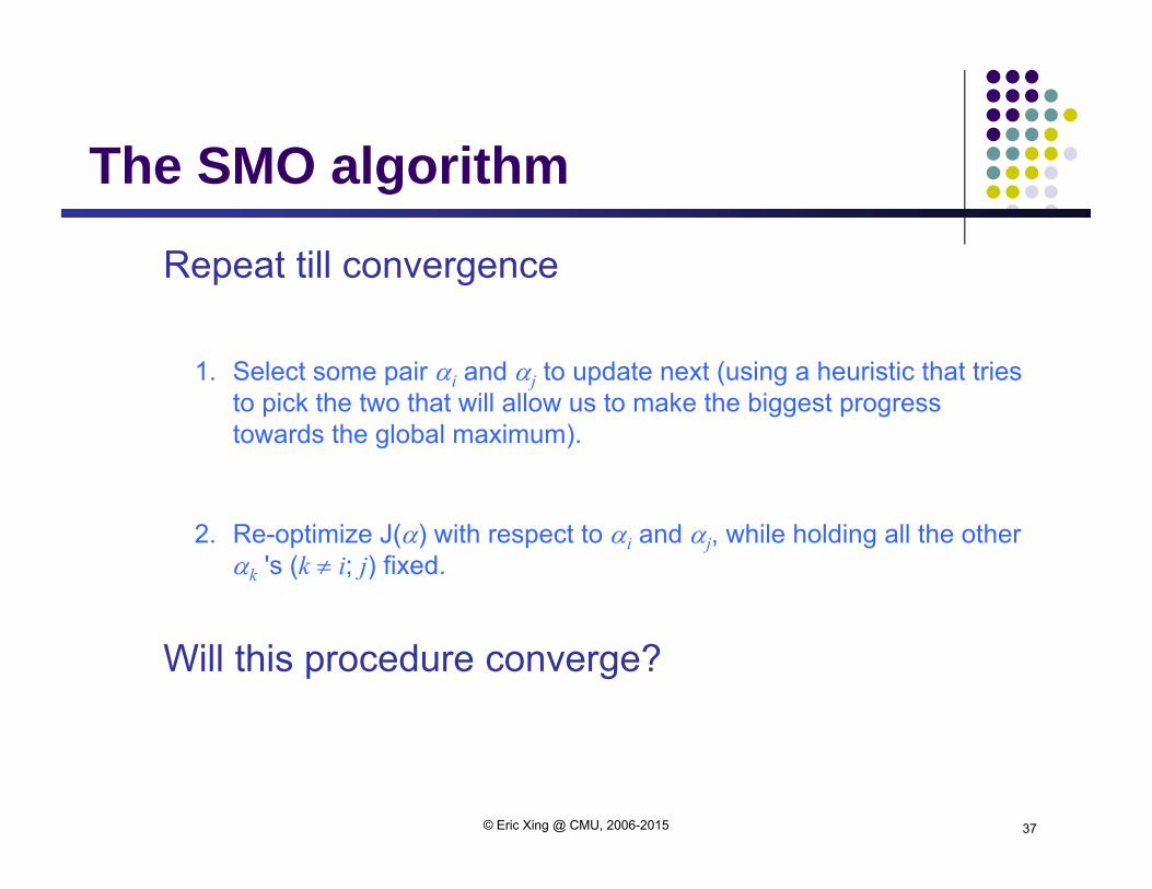
The SMO algorithm
Repeat till convergence
1. Select some pair i and j to update next (using a heuristic that tries to pick the two that will allow us to make the biggest progress towards the global maximum).
2. Re-optimize J() with respect to i and j, while holding all the other k 's (k i; j) fixed.
Will this procedure converge?
© Eric Xing @ CMU, 2006-2015

38
Convergence of SMO
Let’s hold 3 ,…, m fixed and reopt J w.r.t. 1 and 2
m
jij
Tijiji
m
ii yy
1,1)(
21)(max xx J
.
,, ,0 s.t.
m
iii
i
y
kiC
10
1
KKT:
© Eric Xing @ CMU, 2006-2015

39
Convergence of SMO The constraints:
The objective:
Constrained opt:
© Eric Xing @ CMU, 2006-2015

40
Cross-validation error of SVM The leave-one-out cross-validation error does not depend on
the dimensionality of the feature space but only on the # of support vectors!
examples trainingof #ctorssupport ve #error CVout -one-Leave
© Eric Xing @ CMU, 2006-2015

41
Summary Max-margin decision boundary
Constrained convex optimization
Duality
The KTT conditions and the support vectors
Non-separable case and slack variables
The kernel trick
The SMO algorithm
© Eric Xing @ CMU, 2006-2015