support vector machines - university of...
TRANSCRIPT

Support Vector Machines
www.cs.wisc.edu/~dpage
1

Goals for the lecture you should understand the following concepts
• the margin • slack variables • the linear support vector machine • nonlinear SVMs • the kernel trick • the primal and dual formulations of SVM learning • support vectors • the kernel matrix • valid kernels • polynomial kernel • Gausian kernel • string kernels • support vector regression
2

Algorithm You Should Know
• SVM as constrained optimization – Fit training data and maximize margin – Primal and dual formulations – Kernel trick – Slack variables to allow imperfect fit – For now, assuming optimizer is black box
• Next lecture will look inside black box: sequential minimal optimization (SMO)
3

Burr Settles, UW CS PhD 4

Four key SVM ideas • Maximize the margin
don’t choose just any separating hyperplane
• Penalize misclassified examples use soft constraints and slack variables
• Use optimization methods to find model
linear programming quadratic programming
• Use kernels to represent nonlinear functions and handle complex instances (sequences, trees, graphs, etc.)
5

Some key vector concepts
w ⋅x = wTx = wixi
i∑
the dot product between two vectors w and x is defined as:
13−5
"
#
$$$
%
&
'''
⋅4−2−1
"
#
$$$
%
&
'''
= (1)(4)+ (3)(−2)+ (−5)(−1) = 3
for example
x 2 = xi2
i∑
the 2-norm (Euclidean length) of a vector x is defined as:
6

Linear separator learning revisited
h(x) = 1 if wii=1
n
∑ xi"
#$%
&'+ b > 0
−1 otherwise
)
*+
,+
y(wTx + b) > 0
an instance 〈x, y〉 will be classified correctly if
suppose we encode our classes as {-1, +1} and consider a linear classifier
x1
x2
7

Large margin classification • Given a training set that is linearly separable, there are infinitely many
hyperplanes that could separate the positive/negative instances. • Which one should we choose?
• In SVM learning, we find the hyperplane that maximizes the margin.
Figure from Ben-Hur & Weston, Methods in Molecular Biology 2010
8

Large margin classification • suppose we learn a hyperplane h given a training set D • let x+ denote the closest instance to the hyperplane among positive
instances, and similarly for x- and negative instances • the margin is given by
marginD (h) =
12wT x+ − x−( ) = 1
w 2
x+
x-
length 1 vector in same direction as w
9
1 2 3 4 5 6 7 8 9 10 11 12 13 14 15 16 17 18 19
1
2
3
4
5
6
7
8
9
10
11
1
2
13
1
4
-19 -18 -17 -16 -15 -14 -13 -12 -11 -10 -9 -8 -7 -6 -5 -4 -3 -2 -1
-14
-1
3 -
12
-11
-1
0
-9
-8
-
7
-6
-5
-4
-3
-2
-1
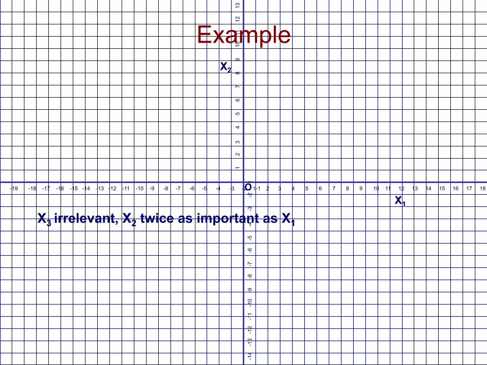
O X1
X2
X3 irrelevant, X2 twice as important as X1
Example

1 2 3 4 5 6 7 8 9 10 11 12 13 14 15 16 17 18 19
1
2
3
4
5
6
7
8
9
10
11
1
2
13
1
4
-19 -18 -17 -16 -15 -14 -13 -12 -11 -10 -9 -8 -7 -6 -5 -4 -3 -2 -1
-14
-1
3 -
12
-11
-1
0
-9
-8
-
7
-6
-5
-4
-3
-2
-1
O X1
X2
X3 irrelevant, X2 twice as important as X1
Example

1 2 3 4 5 6 7 8 9 10 11 12 13 14 15 16 17 18 19
1
2
3
4
5
6
7
8
9
10
11
1
2
13
1
4
-19 -18 -17 -16 -15 -14 -13 -12 -11 -10 -9 -8 -7 -6 -5 -4 -3 -2 -1
-14
-1
3 -
12
-11
-1
0
-9
-8
-
7
-6
-5
-4
-3
-2
-1
O X1
X2
2X2 + X1 – 2 ≥ 0
X3 irrelevant, X2 twice as important as X1
Separator is perpendicular to weight vector

1 2 3 4 5 6 7 8 9 10 11 12 13 14 15 16 17 18 19
1
2
3
4
5
6
7
8
9
10
11
1
2
13
1
4
-19 -18 -17 -16 -15 -14 -13 -12 -11 -10 -9 -8 -7 -6 -5 -4 -3 -2 -1
-14
-1
3 -
12
-11
-1
0
-9
-8
-
7
-6
-5
-4
-3
-2
-1
O X1
X2
2X2 + X1 – 6 ≥ 0
X3 irrelevant, X2 twice as important as X1
Changing b moves (shifts) separator

1 2 3 4 5 6 7 8 9 10 11 12 13 14 15 16 17 18 19
1
2
3
4
5
6
7
8
9
10
11
1
2
13
1
4
-19 -18 -17 -16 -15 -14 -13 -12 -11 -10 -9 -8 -7 -6 -5 -4 -3 -2 -1
-14
-1
3 -
12
-11
-1
0
-9
-8
-
7
-6
-5
-4
-3
-2
-1
O X1
X2
Assume labeled data as above
Size of w, b sensitive to data scaling
+
+ -

1 2 3 4 5 6 7 8 9 10 11 12 13 14 15 16 17 18 19
1
2
3
4
5
6
7
8
9
10
11
1
2
13
1
4
-19 -18 -17 -16 -15 -14 -13 -12 -11 -10 -9 -8 -7 -6 -5 -4 -3 -2 -1
-14
-1
3 -
12
-11
-1
0
-9
-8
-
7
-6
-5
-4
-3
-2
-1
O X1
X2
2X2 + X1 – 4 ≥ 0
X3 irrelevant, X2 twice as important as X1
2X2 + X1 – 2 ≥ 0
Margin is width between our earlier lines
2X2 + X1 – 6 ≥ 0
+
+ -
1 2 3 4 5 6 7 8 9 10 11 12 13 14 15 16 17 18 19
1
2
3
4
5
6
7
8
9
10
11
1
2
13
1
4
-19 -18 -17 -16 -15 -14 -13 -12 -11 -10 -9 -8 -7 -6 -5 -4 -3 -2 -1
-14
-1
3 -
12
-11
-1
0
-9
-8
-
7
-6
-5
-4
-3
-2
-1
O X1
X2
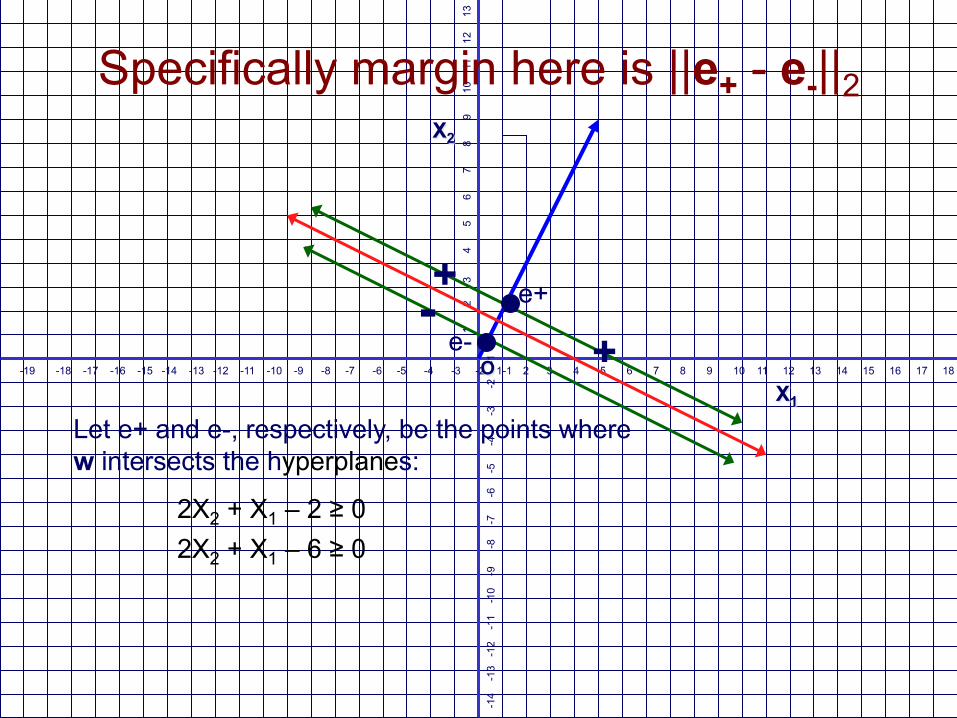
Let e+ and e-, respectively, be the points where w intersects the hyperplanes:
Specifically margin here is ||e+ - e-||2
+
+ -
e-
e+
2X2 + X1 – 2 ≥ 0 2X2 + X1 – 6 ≥ 0

1 2 3 4 5 6 7 8 9 10 11 12 13 14 15 16 17 18 19
1
2
3
4
5
6
7
8
9
10
11
1
2
13
1
4
-19 -18 -17 -16 -15 -14 -13 -12 -11 -10 -9 -8 -7 -6 -5 -4 -3 -2 -1
-14
-1
3 -
12
-11
-1
0
-9
-8
-
7
-6
-5
-4
-3
-2
-1
O X1
X2
2X2 + X1 – 8 ≥ 0
But can double margin artificially
+
+
-
2X2 + X1 – 4 = 0 2X2 + X1 – 12 = 0
e+
e-
OR… 4X2 + 2X1 – 4 ≥ 0
4X2 + 2X1 – 2 = 0 4X2 + 2X1 – 6 = 0
Keep w fixed, double b Double w, keep b fixed

1 2 3 4 5 6 7 8 9 10 11 12 13 14 15 16 17 18 19
1
2
3
4
5
6
7
8
9
10
11
1
2
13
1
4
-19 -18 -17 -16 -15 -14 -13 -12 -11 -10 -9 -8 -7 -6 -5 -4 -3 -2 -1
-14
-1
3 -
12
-11
-1
0
-9
-8
-
7
-6
-5
-4
-3
-2
-1
O X1
X2
But normalized margin remains unchanged: ||e+ – e-||2 / ||w||2 Can keep ||w||2 fixed and try to maximize ||e+ – e-||2 Or fix ||e+ – e-||2 (e.g., to 2) and minimize ||w||2
Should normalize margin with norm of w
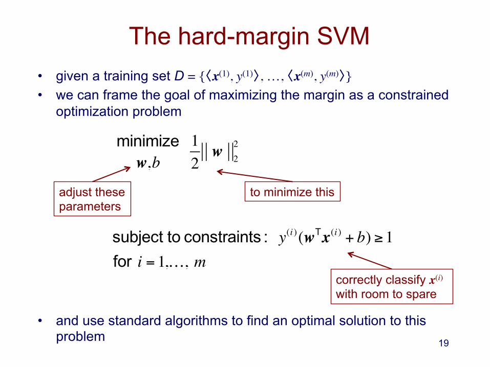
The hard-margin SVM
subject to constraints : y(i )(wTx(i ) + b) ≥1 for i = 1,…, m
minimizew,b
12
w 22
• given a training set D = {〈x(1), y(1)〉, …, 〈x(m), y(m)〉} • we can frame the goal of maximizing the margin as a constrained
optimization problem
adjust these parameters
to minimize this
• and use standard algorithms to find an optimal solution to this problem
correctly classify x(i) with room to spare
19

The soft-margin SVM [Cortes & Vapnik, Machine Learning 1995]
• if the training instances are not linearly separable, the previous formulation will fail
• we can adjust our approach by using slack variables (denoted by ξ) to tolerate errors
subject to constraints : y(i )(wTx(i ) + b) ≥1−ξ (i )
ξ (i ) ≥ 0 for i = 1,…, m
minimizew,b,ξ (1)…ξ (m )
12
w 22+C ξ (i )
i=1
m
∑
• C determines the relative importance of maximizing margin vs. minimizing slack
20

The effect of C in a soft-margin SVM
Figure from Ben-Hur & Weston, Methods in Molecular Biology 2010
21

Nonlinear classifiers
22
-1
+1
x1
x2

Nonlinear classifiers
23
+1
-1 x2
x1
x1x2

Nonlinear classifiers
24
+1
-1 x2
x1
x1x2

Nonlinear classifiers
25
+1
-1 y
x1
xy

Nonlinear classifiers
26
+1
-1 y
x1
xy

Nonlinear classifiers
27
+1
-1 y
x1
xy

Nonlinear classifiers
28
-1
+1
x1
x2

Nonlinear classifiers
• What if a linear separator is not an appropriate decision boundary for a given task?
• For any (consistent) data set, there exists a mapping ϕ to a higher-dimensional space such that the data is linearly separable
φ(x) = φ1(x), φ2 (x), …, φk (x)( )• Example: mapping to quadratic space
x = x1, x2
φ(x) = x12, 2x11x2, x2
2, 2x11, 2x2, 1( )suppose x is represented by 2 features
• now try to find a linear separator in this space
29

Nonlinear classifiers
• for the linear case, our discriminant function was given by
• for the nonlinear case, it can be expressed as
where w is a higher dimensional vector
h(x) = 1 if w ⋅x + b > 0−1 otherwise
#$%
h(x) = 1 if w ⋅φ(x)+ b > 0−1 otherwise
$%&
'&
30

SVMs with polynomial kernels
Figure from Ben-Hur & Weston, Methods in Molecular Biology 2010
31

The kernel trick • explicitly computing this nonlinear mapping does not scale well • a dot product between two higher-dimensional mappings can
sometimes be implemented by a kernel function • example: quadratic kernel
k(x, z) = x ⋅ z +1( )2
= x1z1 + x2z2 +1( )2
= x12z1
2 + 2x1x2z1z2 + x22z2
2 + 2x1z1 + 2x2z2 +1
= x12, 2x1x2, x2
2, 2x1, 2x2, 1( ) i z1
2, 2z1z2, z22, 2z1, 2z2, 1( )
= φ(x) ⋅φ(z)32
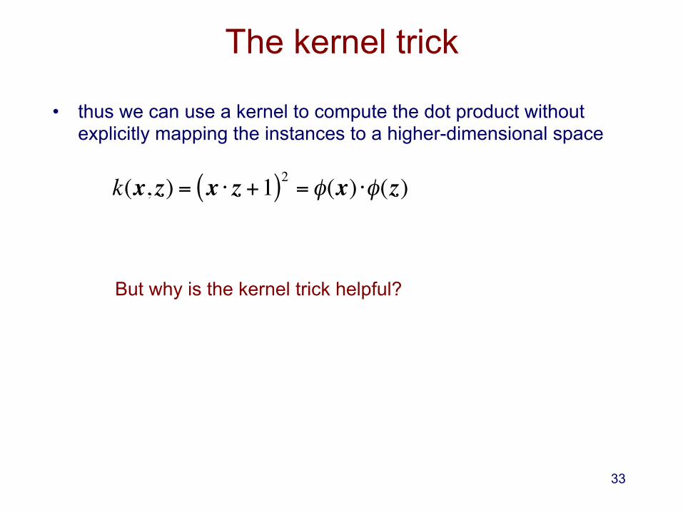
The kernel trick
• thus we can use a kernel to compute the dot product without explicitly mapping the instances to a higher-dimensional space
k(x, z) = x ⋅ z +1( )2 = φ(x) ⋅φ(z)
But why is the kernel trick helpful?
33

Using the kernel trick • given a training set D = {〈x(1), y(1)〉, …, 〈x(m), y(m)〉} • suppose the weight vector can be represented as a linear
combination of the training instances
w = α ii=1
m
∑ x(i )
α i
i=1
m
∑ x(i ) i x + b
• then we can represent a linear SVM as
α ii=1
m
∑ φ x(i )( ) iφ x( ) + b
= α ii=1
m
∑ k x(i ),x( ) + b
• and a nonlinear SVM as
34

Can we represent a weight vector as a linear combination of training instances?
• consider perceptron learning, where each weight can be represented as
wj = α ii=1
m
∑ x j(i )
• proof: each weight update has the form wj (t) = wj (t −1)+ηδ t(i )y(i )x j
(i )
δ t(i ) =
1 if x(i ) misclassified in epoch t0 otherwise
"#$
%$wj = ηδ t
(i )y(i )x j(i )
i=1
m
∑t∑
wj = ηδ t(i )y(i )
t∑$
%&'
()i=1
m
∑ x j(i )
wj = α ii=1
m
∑ x j(i )
35

The primal and dual formulations of the hard-margin SVM
subject to constraints : y(i )(wTx(i ) + b) ≥1 for i = 1,…, m
minimizew,b
12
w 22primal
maximizeα1,…,αm
α ii=1
m
∑ −12
α jα k y( j )y(k ) x( j ) i x(k )( )
k=1
m
∑j=1
m
∑
subject to constraints : α i ≥ 0 for i = 1,…, m
α i y(i )
i=1
m
∑ = 0
dual
36

The dual formulation with a kernel (hard margin version)
subject to constraints : y(i )(wTφ x(i )( ) + b) ≥1
for i = 1,…, m
minimizew,b
12
w 22primal
maximizeα1,…,αm
α ii=1
m
∑ −12
α jα k y( j )y(k )k x( j ), x(k )( )
k=1
m
∑j=1
m
∑
subject to constraints : α i ≥ 0 for i = 1,…, m
α i y(i )
i=1
m
∑ = 0
dual
37

Support vectors • the final solution is a sparse linear combination of the training instances • those instances having αi > 0 are called support vectors – they lie on
the margin boundary • the solution wouldn’t change if all the instances with αi = 0 were deleted
support vectors
38

The kernel matrix
• the kernel matrix (a.k.a. Gram matrix) represents pairwise similarities for instances in the training set
k(x(1),x(1) ) k(x(1),x(2) ) k(x(1),x(m ) )k(x(2),x(1) )
k(x(m ),x(1) ) k(x(m ),x(m ) )
!
"
#####
$
%
&&&&&
• it represents the information about the training set that is provided as input to the optimization process
39

Some common kernels
• polynomial of degree d
• radial basis function (RBF) (a.k.a. Gaussian)
k(x, z) = x ⋅ z +1( )d
k(x, z) = x ⋅ z( )d
k(x, z) = exp −γ x − z 2( )
• polynomial of degree up to d
40

The RBF kernel • the feature mapping ϕ for the RBF kernel is infinite dimensional!
• recall that k(x, z) = ϕ(x) � ϕ (z)
k(x, z) = exp −12x − z 2"
#$%&'
for γ = 12
= exp −12x 2"
#$%&'exp −
12z 2"
#$%&'exp x ⋅ z( )
= exp −12x 2"
#$%&'exp −
12z 2"
#$%&'
x ⋅ z( )n
n!n=0
∞
∑"
#$
%
&'
from the Taylor series expansion of exp(x � z) 41

The RBF kernel illustrated
γ = −10 γ = −1000γ = −100
Figures from openclassroom.stanford.edu (Andrew Ng)
42

What makes a valid kernel?
• k(x, z) is a valid kernel if there is some ϕ such that
k(x, z) = φ(x) ⋅φ(z)
• this holds for a symmetric function k(x, z) if and only if the kernel matrix K is positive semidefinite for any training set (Mercer’s theorem)
∀v :vTKv ≥ 0definition of positive semidefinite (p.s.d):
43

Support vector regression
• the SVM idea can also be applied in regression tasks • an ε-insensitive error function specifies that a training instance
is well explained if the model’s prediction is within ε of y(i)
y(i ) − wTx(i ) + b( ) = ε
wTx(i ) + b( )− y(i ) = ε
44
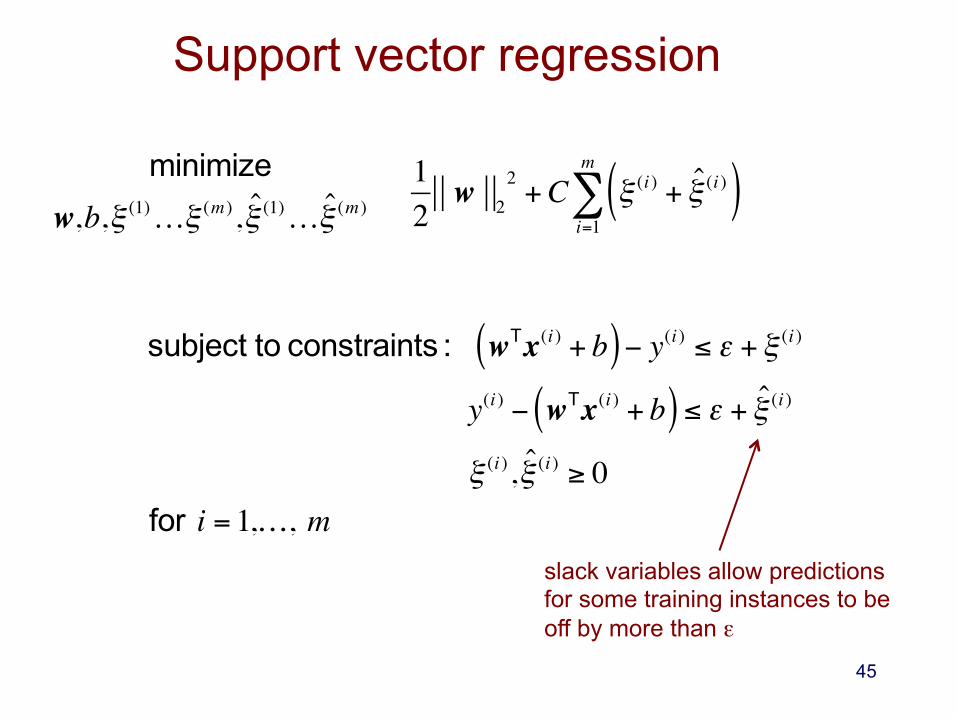
Support vector regression
subject to constraints : wTx(i ) + b( )− y(i ) ≤ ε + ξ (i )
y(i ) − wTx(i ) + b( ) ≤ ε + ξ (i )
ξ (i ),ξ (i ) ≥ 0 for i = 1,…, m
minimizew,b,ξ (1)…ξ (m ),ξ (1)…ξ (m ) 1
2 w 2
2+C ξ (i ) + ξ (i )( )
i=1
m
∑
slack variables allow predictions for some training instances to be off by more than ε
45
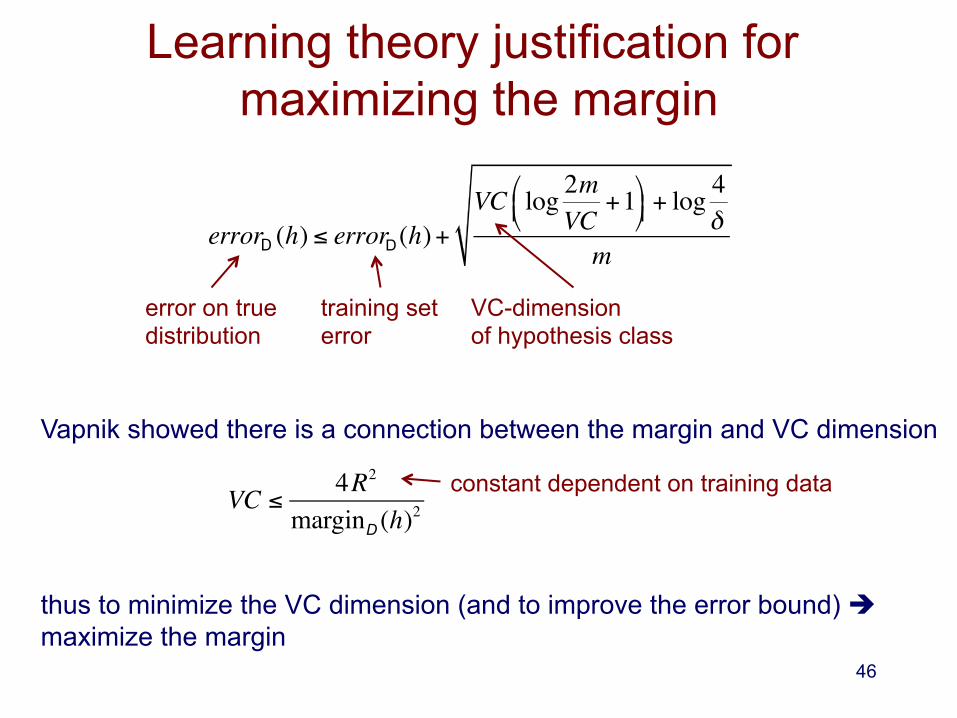
Learning theory justification for maximizing the margin
errorD (h) ≤ errorD(h)+
VC log 2mVC
+1"#$
%&'+ log 4
δm
error on true distribution
training set error
VC-dimension of hypothesis class
thus to minimize the VC dimension (and to improve the error bound) è maximize the margin
VC ≤
4R2
marginD (h)2
Vapnik showed there is a connection between the margin and VC dimension
constant dependent on training data
46

The power of kernel functions
• kernels can be designed and used to represent complex data types such as • strings • trees • graphs • etc.
• let’s consider a specific example
47

The protein classification task
Given: amino-acid sequence of a protein Do: predict the family to which it belongs
GDLSTPDAVMGNPKVKAHGKKVLGAFSDGLAHLDNLKGTFATLSELHCDKLHVDPENFRLLGNVCVLAHHFGKEFTPPVQAAYAKVVAGVANALAHKYH
48

The k-spectrum feature map
• we can represent sequences by counts of all of their k-mers
x = AKQDYYYYEI
ϕ(x) =( 0 , 0 , … , 1 , … , 1 , … , 2 ) AAA AAC … AKQ … DYY … YYY
• the dimension of ϕ(x) = |A|k where |A| is the size of the alphabet • using 6-mers for protein sequences, |20|6 = 64 million • almost all of the elements in ϕ(x) are 0 since a sequence of
length l has at most l-k+1 k-mers
k = 3
49

The k-spectrum kernel
• consider the k-spectrum kernel applied to x and z with k = 3
x = AKQDYYYYEI
ϕ(x) =( 0 , … , 1 , … , 1 , … , 0 ) AAA … AKQ … YEI … YYY
z = AKQIAKQYEI
ϕ(x) � ϕ(z) = 2 + 1 = 3
ϕ(z) =( 0 , … , 2 , … , 1 , … , 0 ) AAA … AKQ … YEI … YYY
50

(k, m)-mismatch feature map
• closely related protein sequences may have few exact matches, but many near matches
• the (k, m)-mismatch feature map uses the k-spectrum representation, but allows up to m mismatches
x = AKQ
ϕ(x) =( 0, … , 1 , … , 1 , … , 1 , … , 0 ) AAA AAQ … AKQ … DKQ … YYY
k = 3, m = 1
51
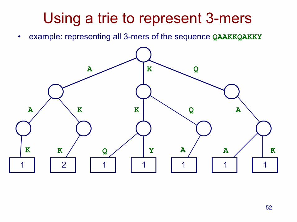
Using a trie to represent 3-mers • example: representing all 3-mers of the sequence QAAKKQAKKY
A K Q
2 1 1 1 1 1 1
A K K Q A
K K Q Y A A K
52

Computing the kernels efficiently with tries [Leslie et al., NIPS 2002]
k-spectrum kernel • for each sequence
– build a trie representing its k-mers • compute kernel ϕ(x) � ϕ(z) by traversing trie for x using k-mers from z
– update kernel function when reaching a leaf
(k, m)-mismatch kernel • for each sequence
• build a trie representing its k-mers and also k-mers with at most m mismatches
• compute kernel ϕ(x) � ϕ(z) by traversing trie for x using k-mers from z – update kernel function when reaching a leaf
O km+1 A m x + z( )( )scales linearly with sequence length: 53
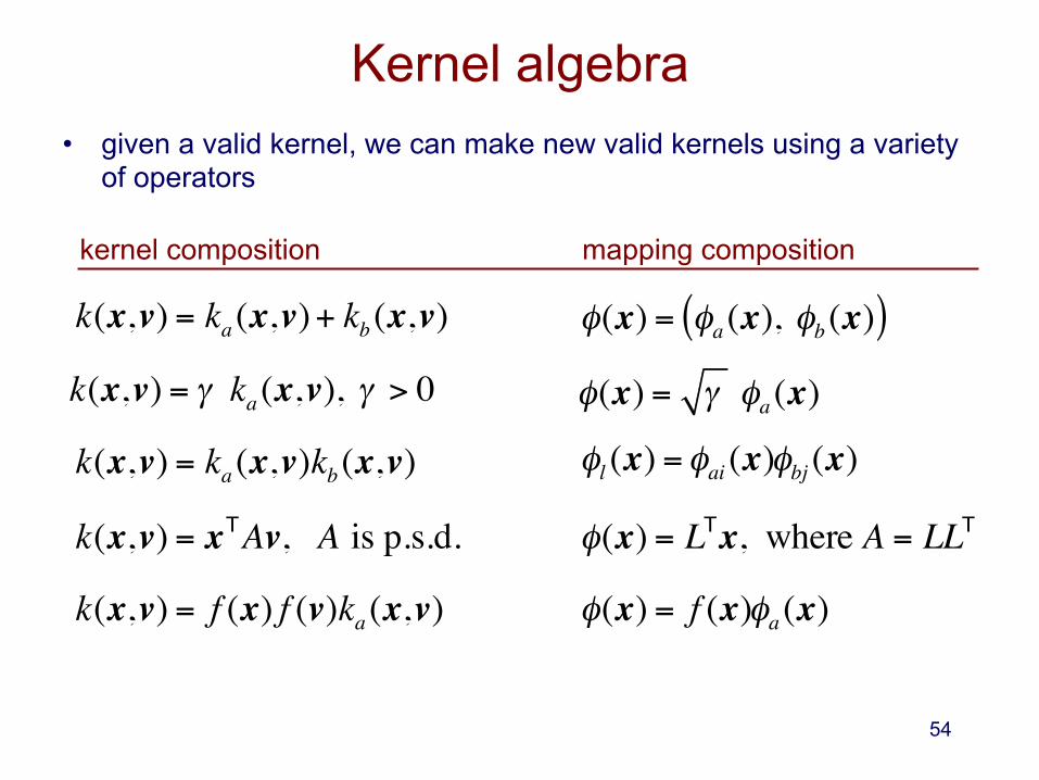
Kernel algebra • given a valid kernel, we can make new valid kernels using a variety
of operators
φ(x) = φa (x), φb (x)( )k(x,v) = ka (x,v)+ kb (x,v)
k(x,v) = γ ka (x,v), γ > 0 φ(x) = γ φa (x)
k(x,v) = ka (x,v)kb (x,v) φl (x) = φai (x)φbj (x)
k(x,v) = xTAv, A is p.s.d. φ(x) = LTx, where A = LLT
k(x,v) = f (x) f (v)ka (x,v) φ(x) = f (x)φa (x)
kernel composition mapping composition
54
Comments on SVMs
• we can find solutions that are globally optimal (maximize the margin) • because the learning task is framed as a convex optimization
problem • no local minima, in contrast to multi-layer neural nets
• there are two formulations of the optimization: primal and dual • dual represents classifier decision in terms of support vectors • dual enables the use of kernel functions
• we can use a wide range of optimization methods to learn SVM • standard quadratic programming solvers • SMO [Platt, 1999] • linear programming solvers for some formulations • etc.
55

Comments on SVMs • kernels provide a powerful way to
• allow nonlinear decision boundaries
• represent/compare complex objects such as strings and trees
• incorporate domain knowledge into the learning task
• using the kernel trick, we can implicitly use high-dimensional mappings without explicitly computing them
• one SVM can represent only a binary classification task; multi-class problems handled using multiple SVMs and some encoding
• one class vs. rest
• ECOC
• etc.
• empirically, SVMs have shown state-of-the art accuracy for many tasks
• the kernel idea can be extended to other tasks (anomaly detection, regression, etc.) 56