www.sciencemag.org/cgi/content/full/320/5880/1191/DC1

Supporting Online Material for

Predicting Human Brain Activity

Associated with the Meanings of Nouns

Tom M. Mitchell,* Svetlana V. Shinkareva, Andrew Carlson, Kai-Min Chang, Vicente L. Malave, Robert A. Mason, Marcel Adam Just

*To whom correspondence should be addressed. E-mail: Tom.Mitchell@cs.cmu.edu

Published 30 May 2008, Science 320, 1191 (2008)

DOI: 10.1126/science.1152876

This PDF file includes:

Materials and Methods SOM Text Figs. S1 to S5 References

Predicting Human Brain Activity Associated with the Meanings of Nouns

Tom M. Mitchell, Svetlana V. Shinkareva, Andrew Carlson, Kai-Min Chang, Vicente L. Malave, Robert A. Mason, Marcel Adam Just

Science, vol. 320

May 30, 2008.

Supporting online material

Table of Contents

1. Materials and Methods .............................................................................................................................. 3

1.1 fMRI Data collection and processing .................................................................................................. 3

1.2 Text corpus data .................................................................................................................................. 4

1.3 Training the model .............................................................................................................................. 4

1.4 Training and Evaluating Computational Models ................................................................................ 5

1.5 Matching predicted to actual images .................................................................................................. 5

1.6 Voxel selection .................................................................................................................................... 5

1.7 Empirical distribution to determine statistical significance and p values ........................................... 6

1.8 Computing the accuracy map of Figure 3 in the main paper .............................................................. 7

2. Additional Results and Observations ........................................................................................................ 8

2.1 Experiment with randomly generated intermediate semantic features ............................................... 8

2.2 Learned Feature Signatures ................................................................................................................. 9

2.3 Plot of similarities between predicted and actual images ................................................................... 9

2.4 Resolving among 1000 candidate words........................................................................................... 10

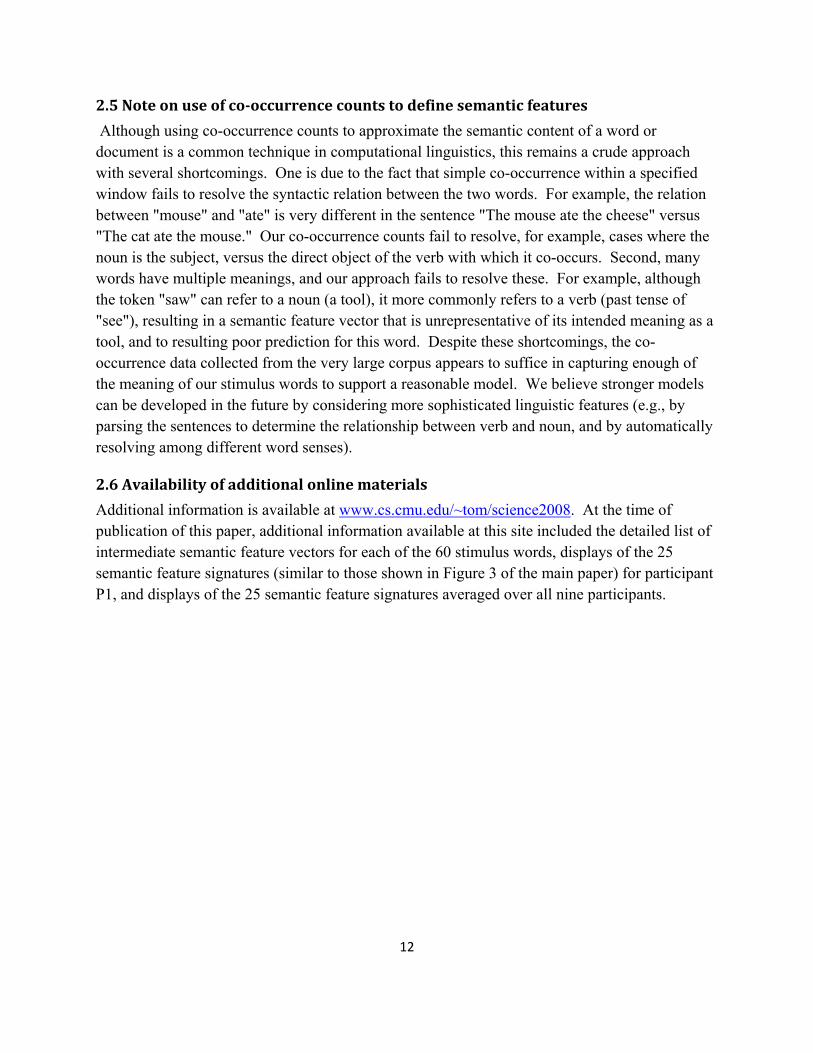
2.5 Note on use of co-occurrence counts to define semantic features .................................................... 12

2.6 Availability of additional online materials ........................................................................................ 12

3. Additional Figures and legends ............................................................................................................... 13

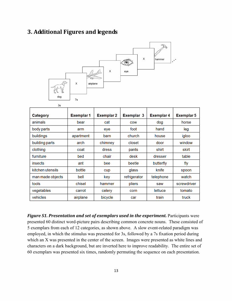
Figure S1. Presentation and set of exemplars used in the experiment. ................................................... 13

2 

 

Figure S2. Empirical distribution of accuracies for null models, and Gaussian approximation. ............ 14

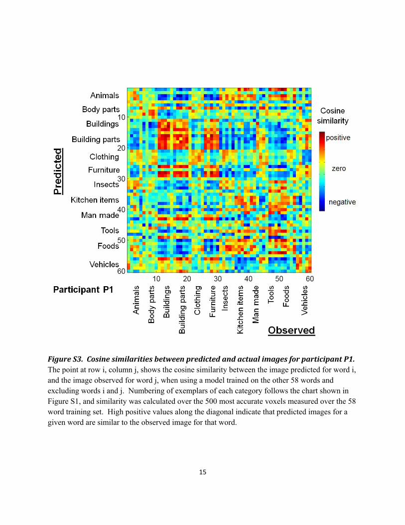
Figure S3. Cosine similarities between predicted and actual images for participant P1. ....................... 15

Figure S4. Cosine similarities between predicted and actual images, averaged over all participants. .. 16

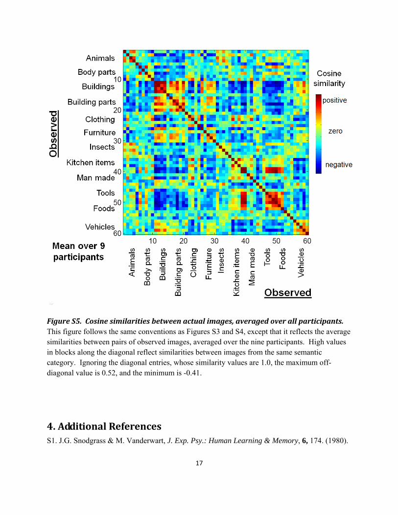
Figure S5. Cosine similarities between actual images, averaged over all participants. ......................... 17

4. Additional References ............................................................................................................................. 17

 

3 

 

1. Materials and Methods 

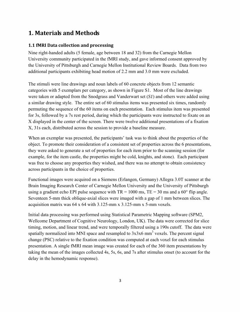
1.1 fMRI Data collection and processing 

Nine right-handed adults (5 female, age between 18 and 32) from the Carnegie Mellon University community participated in the fMRI study, and gave informed consent approved by the University of Pittsburgh and Carnegie Mellon Institutional Review Boards. Data from two additional participants exhibiting head motion of 2.2 mm and 3.0 mm were excluded. The stimuli were line drawings and noun labels of 60 concrete objects from 12 semantic categories with 5 exemplars per category, as shown in Figure S1. Most of the line drawings were taken or adapted from the Snodgrass and Vanderwart set (S1) and others were added using a similar drawing style. The entire set of 60 stimulus items was presented six times, randomly permuting the sequence of the 60 items on each presentation. Each stimulus item was presented for 3s, followed by a 7s rest period, during which the participants were instructed to fixate on an X displayed in the center of the screen. There were twelve additional presentations of a fixation X, 31s each, distributed across the session to provide a baseline measure.  

When an exemplar was presented, the participants’ task was to think about the properties of the object. To promote their consideration of a consistent set of properties across the 6 presentations, they were asked to generate a set of properties for each item prior to the scanning session (for example, for the item castle, the properties might be cold, knights, and stone). Each participant was free to choose any properties they wished, and there was no attempt to obtain consistency across participants in the choice of properties.

Functional images were acquired on a Siemens (Erlangen, Germany) Allegra 3.0T scanner at the Brain Imaging Research Center of Carnegie Mellon University and the University of Pittsburgh using a gradient echo EPI pulse sequence with TR = 1000 ms, TE = 30 ms and a 60° flip angle. Seventeen 5-mm thick oblique-axial slices were imaged with a gap of 1 mm between slices. The acquisition matrix was 64 x 64 with 3.125-mm x 3.125-mm x 5-mm voxels.

Initial data processing was performed using Statistical Parametric Mapping software (SPM2, Wellcome Department of Cognitive Neurology, London, UK). The data were corrected for slice timing, motion, and linear trend, and were temporally filtered using a 190s cutoff. The data were spatially normalized into MNI space and resampled to 3x3x6 mm3 voxels. The percent signal change (PSC) relative to the fixation condition was computed at each voxel for each stimulus presentation. A single fMRI mean image was created for each of the 360 item presentations by taking the mean of the images collected 4s, 5s, 6s, and 7s after stimulus onset (to account for the delay in the hemodynamic response).

4 

 

1.2 Text corpus data 

The text corpus data was provided by Google Inc., and is available online at http://www.ldc.upenn.edu/Catalog/CatalogEntry.jsp?catalogId=LDC2006T13. It consists of a set of n-grams (sequences of words and other text tokens) ranging from unigrams (single tokens) up to five-grams (sequences of five tokens), along with counts giving the number of times each n-gram appeared in a large corpus containing over a trillion total tokens. The corpus consisted of publicly available English text web pages. N-grams occurring fewer than 40 times were not provided. We used this data to calculate co-occurrence counts for words occurring within five tokens of one another. These are the co-occurrence counts used in all experiments reported in this paper.

1.3 Training the model 

Once the semantic features fi(w) are specified, the parameters cvi that define the neural signature contributed by the ith semantic feature to the vth voxel are estimated. This is accomplished by training the model using a set of observed fMRI images associated with known stimulus words. Each training stimulus wt is first re-expressed in terms of its feature vector < f1(wt) … fn(wt) >, and multiple regression is then used to obtain maximum likelihood estimates of the cvi values; that is, the set of cvi values that minimize the sum of squared errors in reconstructing the training fMRI images. If the number of semantic features is less than the number of training examples, then this multiple regression problem is well posed and a unique solution is obtained. If the number of semantic features is greater than the number of training examples, a solution can be obtained by introducing a regularization term such as a penalty equal to the sum of squares of the learned regression weights.

Once trained, the resulting computational model can be used to predict the full fMRI activation image for any other word found in the trillion (1012) token text corpus, as shown in Figure 2A of the main text. Given an arbitrary new word wnew the model first extracts the intermediate semantic feature values < f1(wnew) … fn(wnew) > from the corpus statistics database, then applies the above formula using the previously learned values for the parameters cvi. The computational model and corresponding theory can be directly evaluated by comparing their predictions for words outside the training set to observed fMRI images associated with those words. Different predefined sets of intermediate semantic features can be directly compared by training competing models and evaluating their prediction accuracies.

The detailed list of intermediate semantic features vectors for each of the 60 stimulus words can be found at www.cs.cmu.edu/~tom/science2008.

5 

 

1.4 Training and Evaluating Computational Models 

Alternative computational models were trained based on different sets of intermediate semantic features. Each model was trained and evaluated using a cross validation approach, in which the model was repeatedly trained using only 58 of the 60 available stimulus items, then tested using the two stimulus items that had been left out. On each iteration, the trained model was tested by giving it the two stimulus words it had not yet seen (w1 and w2), plus their observed fMRI images (i1 and i2), then requiring it to predict which of the two novel images was associated with which of the two novel words, using a matching procedure described in the following section. This leave-two-out train-test procedure was iterated 1770 times, leaving out each of the possible word pairs. The expected accuracy in matching the two left-out words to their left-out fMRI images is 0.50 if the matching is performed at chance levels.

1.5 Matching predicted to actual images 

Given a trained computational model, two new words (w1 and w2) and two new images (i1 and i2), the trained model was first used to create predicted image p1 for word w1 and predicted image p2 for word w2. It then decided which was a better match: (p1=i1 and p2=i2) or (p1=i2 and p2=i1), by choosing the image pairing with the best similarity score. Because we do not expect every voxel in the brain to be involved in representing the meaning of the stimulus, only a subset of voxels was used for assessing the similarity between images. This subset of voxels was selected automatically during training, using only the data for the 58 training words, and excluding the data from the two test words. The voxel selection method is described below. Let sel(i) be the vector of values of the selected subset of voxels for image i. The similarity score between a predicted image, p, and observed image, i, was calculated as the cosine similarity between the vectors sel(p) and sel(i). Cosine similarity between two vectors is defined as the cosine of the angle between the vectors, and was computed as the dot product of these vectors normalized to unit length. Finally, the similarity match score for a candidate pairing of predicted to actual images, (e.g., p1=i2 and p2=i1), was computed as the sum of the two cosine similarities:

match(p1=i2 and p2=i1) = cosineSimilarity(sel(p1),sel(i2))+cosineSimilarity(sel(p2),sel(i1)).

Cosine similarity was the first similarity measure we considered, but we subsequently also considered the Pearson correlation between two images and found that the two yielded similar results. All results reported in the current paper use cosine similarity.

1.6 Voxel selection  

As described above, similarity between two images was calculated using only a subset of the image voxels. Voxels were selected automatically during training, using only the 58 training words on each of the leave-two-out cross validation folds. To select voxels, all voxels were first

6 

 

assigned a "stability score" using the data from the 6 presentations of each of the 58 training stimuli. Given these 6 x 58 = 348 presentations represented as 348 fMRI images, each voxel was assigned a 6x58 matrix, where the entry at row i, column j, is the value of this voxel during the ith presentation of the jth word. The stability score for this voxel was then computed as the average pairwise correlation over all pairs of rows in this matrix. In essence, this assigns highest scores to voxels that exhibit a consistent (across different presentations) variation in activity across the 58 training stimuli. For example, if a voxel were to exhibit the same 58 responses during each presentation, it would have an average pairwise correlation of 1.0. Of course the noise inherent in fMRI activations prevents this from happening in practice, and high pairwise correlations tend to be found only when there is a strong and repeatable voxel response pattern of signals that outweighs this noise. Note that high pairwise correlations can occur even among voxels that activate similarly for some of the 58 stimuli, so long as they activate differently (and consistently so) for at least some other subset of the 58 stimuli. The 500 voxels ranked highest by this stability score were used in the cosine similarity test described above. Although individual selected voxels might distinguish among only some subset of the stimuli, the entire set of voxels selected in this fashion tends to distinguish fairly well in practice among all stimuli, as is evident from the reported results.

1.7 Empirical distribution to determine statistical significance and p values 

The expected chance accuracy of an uninformed model correctly matching two stimuli outside the training set to their two fMRI images is 0.5. The observed accuracies of our trained models, based on 1770 iterations of a leave-two-out cross validation train/test regime, are higher than 0.5. Here we consider the question of how to determine p values based on observed accuracies, to reject the null hypothesis that the trained model has true accuracy of 0.5. Given our leave-two-out train/test regime, no closed-form formula is available to assign such a p value. Therefore, we computed p values based on an empirical distribution of observed accuracies obtained from 768 independently trained single-participant models that we expect will have true accuracy very close to 0.5. The empirical distribution of accuracies for these null models was 0.501, with standard deviation 0.070, indicating that observed accuracies above 0.62 for a single participant model is statistically significant at p<0.05. Below we describe our approach in more detail.

We created this empirical distribution of accuracies by training multiple models using the observed fMRI images for the 60 stimulus words, but using different word labels and different intermediate semantic features. This approach is similar to a form of permutation test, except that instead of permuting the 60 stimulus labels, we chose 60 new words from the vocabulary of tokens in our text corpus. In particular, each model was trained by first choosing one of our nine participant data sets uniformly at random, then selecting 60 words uniformly at random from the 500 through 5000 most frequent words in the text corpus, then selecting 25 intermediate semantic feature words uniformly at random from the 500 through 5000 most frequent words in the corpus. The model was then trained and tested, substituting the 60 randomly drawn words

7 

 

for the 60 correct word labels, and using the 25 randomly drawn intermediate semantic feature words. Models were trained and tested using the leave-two-out test regime, exactly as elsewhere in this paper, with one minor exception: in these models the 500 most stable voxels were selected using data from all 60 words, whereas elsewhere this selection of stable voxels was based only on the 58 training words. This exception was made because it dramatically improves the tractability of training hundreds of such random models, leading to a 1000-fold speedup. Note the net effect is that the expected observed accuracy of the random models evaluated in this way will be slightly positively biased, and the p values calculated from the resulting distribution will therefore be slightly conservative. In fact, we found this bias to be very small, as the empirical mean accuracy of models trained and tested in this way was 0.501, very close to the expected chance accuracy of 0.500.

We trained and tested 768 such randomly generated models. The mean accuracy over these 768 models was 0.501, with standard deviation 0.070. The distribution of observed accuracies is plotted in Figure S2. Examining the cumulative distribution, we found that 95% of these models had accuracies below 0.621, and therefore assign a p value of p<0.05 to single subject models with observed accuracies above 0.621. As a consistency check, we also modeled the empirical distribution of accuracies as a Gaussian with µ=0.501 and σ=0.070, and, based on the cumulative distribution for a Gaussian found that p<0.05 corresponds to accuracies greater than µ+1.645σ = 0.617, which is very close to the 0.621 obtained from the empirical cumulative distribution. Under this same Gaussian model, an accuracy of 0.719 for a single-participant model would be significant at p < .001. Notice the above analysis applies to the accuracy of a single model trained for a single participant. The p value associated with observing that all nine independently trained participant models exhibit accuracies greater than 0.62 is p< 10-11.

1.8 Computing the accuracy map of Figure 3 in the main paper 

The accuracy map in Figure 3 of the main text shows voxel clusters with the highest correlation between predicted and actual voxel values. We first calculated sixty predicted images for the sixty words, training a model on the other 59 words, then using this to predict the remaining word. For each voxel, this produced a set of 60 predicted values. The accuracy score of each voxel was calculated as the Pearson correlation between this vector of its predicted values and the corresponding vector of its observed values. An image map containing these voxel scores was created, and the clusters shown in Figure 3 were then produced using standard SPM tools, to identify clusters containing at least 10 contiguous voxels whose score was greater than a threshold value (0.28 for Figure 3A and 3B, and 0.14 for Figure 3C).

8 

 

2. Additional Results and Observations 

2.1 Experiment with randomly generated intermediate semantic features 

Features in this experiment, summarized in Figure 5 of the main text, were defined by 25 randomly selected words. These 25 words were chosen uniformly at random from the 5000 most frequently occurring tokens in the text corpus, and omitting the 500 most frequent tokens (which include many function words such as "the" and "of") as well as the 60 stimulus nouns. Models were trained and tested exactly as described for our 25 manually selected verbs, with one exception which introduced a slight optimistic bias in the measured accuracy of models trained with these randomly generated features: Instead of performing voxel selection using just the 58 training words on each cross-validation fold, the voxels were instead selected just once for each participant and feature set, using all 60 words. This change was introduced in order to reduce the computational cost of training and testing models, enabling us to explore a larger variety of randomly generated feature sets. As discussed in the above section on "Empirical distribution to determine statistical significance and p values," we estimate that the positive bias in observed accuracies due to performing voxel selection is this way is negligible.

Compared to our manually generated set of 25 semantic features, the randomly generated feature sets differed in two ways worth noting. First, whereas our manually generated features were all verbs, the randomly generated features contained tokens of all kinds, including many adjectives, verbs, adverbs, nouns, proper names, slang words, and some tokens frequently found on the web which may not be commonly thought of as English words (e.g., "html"). Second, whereas we defined the features for our verbs using three forms of the verb (e.g., the feature for the verb "eat" used the sum of co-occurrences with the three forms of the verb "eat," "eats," and "ate"), we did not attempt to expand randomly selected tokens into such sets of related tokens. In general there is no obvious way to automatically expand arbitrary word tokens in an analogous fashion, and for many words (e.g., "partly," "news") it is unclear how to do this even manually.

For each randomly generated feature set, models were trained for each of the nine participants. Among the 115 randomly generated feature sets, the greatest mean accuracy achieved across the nine participants was 0.68, compared to 0.77 for the 25 manually selected verbs. The set of 25 randomly selected feature tokens that achieved this 0.68 accuracy is: seems, productions, lots, various, counts, seek, lab, arizona, body, pieces, drop, disabled, lol, venture, finally, arts, eating, infrastructure, xml, nikon, ericsson, partly, governments, ladies, and ft. The feature set with the lowest nine-participant mean accuracy achieved an accuracy of 0.46. This feature set used the tokens: outcome, sessions, schedule, failure, characteristics, statistics, med, beauty, mt, alternative, richard, responsible, god, parties, candidates, towards, governments, fred, father, seeking, kim, hunt, xxx, keeps, and summary. In scanning the feature sets with higher versus lower accuracies, we found no obvious regularities.

9 

 

2.2 Learned Feature Signatures 

Figure 4 in the main text shows some of the feature signatures for participant P1, and averaged over nine participants. Voxels that were absent in any participant were excluded from the image displaying the mean over participants. The full set of 25 feature signatures for participant P1 and averaged over nine participants is available online at www.cs.cmu.edu/~tom/science2008

2.3 Plot of similarities between predicted and actual images 

To provide more insight into the power of the trained computational model, Figure S3 depicts for participant P1 the cosine similarity score between each of the 60 predicted images and each of the 60 observed images, using the 500 most stable voxels as described above. Here the entry at row i and column j gives the cosine similarity between the predicted image for stimulus word i, and the observed image for word j, using a model trained without either word (training on the other 58 words). Thus, this figure contains only similarity scores between pairs of words outside the training set. Note high positive values along the diagonal indicate correct predictions at the word level. High values in blocks around the diagonal reflect similarities between images from the same semantic category. Note also the dark blue regions generally indicate category pairs where the predicted images for words from category A are very different from (have negative cosine similarity with) category B. Whereas Figure S3 shows the similarities for participant P1, Figure S4 shows the similarities averaged over all nine participants.

Examining the entries in Figure S4, one can determine how well the similarity scores resolve on average the correct word out of the 60 candidates. In particular, each row shows the similarity scores of the predicted word's image to each of the 60 observed images (each calculated by a model that omitted the two words being compared). Sorting these similarity scores for each row from most to least similar, the score of the correct word appears at the 79th percentile on average, indicating an imperfect but strong ability of the model to predict images whose features resolve among the 60 words. The percentile rank of the correct image for each of the 60 words is shown below. Words here are numbered according to their position in Figures S3, S4 and S5.

1. 0.283 bear 2. 0.767 cat 3. 0.517 cow 4. 0.950 dog 5. 0.950 horse 6. 0.750 arm 7. 0.583 eye 8. 0.933 foot 9. 0.883 hand 10. 0.833 leg 11. 0.917 apartment

12. 0.950 barn 13. 0.950 church 14. 0.950 house 15. 0.400 igloo 16. 0.900 arch 17. 0.933 chimney 18. 0.983 closet 19. 0.967 door 20. 0.983 window 21. 0.850 coat 22. 0.967 dress

23. 0.933 pants 24. 0.850 shirt 25. 0.867 skirt 26. 0.717 bed 27. 0.783 chair 28. 0.833 desk 29. 0.833 dresser 30. 0.550 table 31. 0.867 ant 32. 0.900 bee 33. 0.917 beetle

10 

 

34. 0.317 butterfly 35. 0.783 fly 36. 0.983 bottle 37. 0.817 cup 38. 0.983 glass 39. 0.900 knife 40. 0.967 spoon 41. 0.383 bell 42. 0.267 key

43. 0.867 refrigerator 44. 0.283 telephone 45. 0.867 watch 46. 0.883 chisel 47. 0.833 hammer 48. 0.933 pliers 49. 0.067 saw 50. 0.967 screwdriver 51. 0.783 carrot

52. 0.767 celery 53. 0.950 corn 54. 0.567 lettuce 55. 0.150 tomato 56. 0.867 airplane 57. 0.983 bicycle 58. 0.883 car 59. 0.983 train 60. 0.983 truck

Note the word producing the worst prediction above is "saw" (word 49). This is primarily due to the fact that although we presented "saw" to our subjects as a tool, the token co-occurrence counts for "saw" used by the model are dominated by its more frequent use as a verb (past tense of "see"). This suggests that future refinements to our model might achieve even greater accuracy by using an enriched set of corpus features that distinguish different meanings of word tokens.

For comparison to Figure S4, Figure S5 shows the similarities between the sixty observed images (and is therefore a summary of the data, rather than the trained models). More specifically, the entry at row i and column j shows the mean, over the nine participants, of the similarity between the observed images for words i and j for that participant. Comparing Figure S5 to Figure S4, it is possible to see that some of the confusions in the predicted versus actual images (off-diagonal red and yellow entries) are the result of similarities in the actual observed images for the two stimuli, whereas other confusions reflect errors in the model in failing to predict differences that do exist in the actual images. For example, it appears that the similarities visible in Figure S4 between the predicted and observed images for furniture items and building parts may be due to actual similarities between the neural encodings of these objects as seen in Figure 4. In comparing Figures S3, S4 and S5, note the color scale is customized to each figure, setting the brightest red to the maximum in the matrix, and the darkest blue to the minimum.

2.4 Resolving among 1000 candidate words 

As described in the main paper, we also performed a leave-one-out test in which the model was repeatedly trained using 59 of the 60 available stimuli, and was then asked to rank a set of 1001 candidate words according to which candidate was most likely to have produced the held out fMRI image. The ranking was based on the cosine similarity between the held out fMRI image and the predicted images for each of the candidate words (as usual, using only the 500 most stable voxels over the training data). For this experiment we used the 1300 most frequent tokens in the text corpus, omitting the 300 most frequent (which contain many function words such as "for" and "the"). As noted in the main paper, the mean percentile rank of the correct word in the

11 

 

model's ranked list was 0.72 on average, across all nine participants. The median rank accuracy of the correct word across all participants was 0.79, reflecting the fact that most words were ranked fairly highly, and a smaller number were ranked very poorly. Below is the list of all 60 words, sorted by their average percentile rank across all nine participants (the number next to each word is the mean percentile rank of this word in the sorted list of candidates, when it was the correct candidate word). As can be seen, some words, such as "glass" are very accurately predicted on average across all participants, with only 26 of the 1000 candidates on average ranked more likely to have generated the test fMRI image. Other words, such as "saw" and "bear" are ranked very poorly on average. Notice that the accurately and inaccurately ranked words below correlate highly with the words ranked accurately and inaccurately in the list above, associated with Figure S4. The difference between these two lists is that the list below involves ranking 1001 predicted images by their similarity to the single observed fMRI image for the held-out word. In contrast, the list above involves ranking the 60 observed fMRI images by their similarity to the single predicted image for the held-out word. .

1. 0.974 glass 2. 0.955 chimney 3. 0.914 church 4. 0.905 train 5. 0.898 bicycle 6. 0.890 dress 7. 0.889 closet 8. 0.889 screwdriver 9. 0.886 foot 10. 0.884 bottle 11. 0.878 arch 12. 0.868 house 13. 0.856 airplane 14. 0.852 horse 15. 0.851 door 16. 0.849 spoon 17. 0.846 barn 18. 0.837 window 19. 0.825 hammer 20. 0.824 knife

21. 0.822 chisel 22. 0.821 car 23. 0.819 dresser 24. 0.814 skirt 25. 0.810 truck 26. 0.802 leg 27. 0.799 hand 28. 0.796 refrigerator 29. 0.796 bee 30. 0.792 dog 31. 0.791 cup 32. 0.775 watch 33. 0.771 apartment 34. 0.769 pants 35. 0.765 pliers 36. 0.751 desk 37. 0.743 bed 38. 0.743 coat 39. 0.738 corn 40. 0.732 shirt

41. 0.718 carrot 42. 0.703 chair 43. 0.702 ant 44. 0.673 fly 45. 0.668 celery 46. 0.628 arm 47. 0.585 cat 48. 0.585 beetle 49. 0.570 table 50. 0.533 eye 51. 0.512 bell 52. 0.512 key 53. 0.476 cow 54. 0.453 lettuce 55. 0.434 igloo 56. 0.345 tomato 57. 0.307 butterfly 58. 0.295 telephone 59. 0.242 bear 60. 0.171 saw

12 

 

2.5 Note on use of co­occurrence counts to define semantic features 

Although using co-occurrence counts to approximate the semantic content of a word or document is a common technique in computational linguistics, this remains a crude approach with several shortcomings. One is due to the fact that simple co-occurrence within a specified window fails to resolve the syntactic relation between the two words. For example, the relation between "mouse" and "ate" is very different in the sentence "The mouse ate the cheese" versus "The cat ate the mouse." Our co-occurrence counts fail to resolve, for example, cases where the noun is the subject, versus the direct object of the verb with which it co-occurs. Second, many words have multiple meanings, and our approach fails to resolve these. For example, although the token "saw" can refer to a noun (a tool), it more commonly refers to a verb (past tense of "see"), resulting in a semantic feature vector that is unrepresentative of its intended meaning as a tool, and to resulting poor prediction for this word. Despite these shortcomings, the co-occurrence data collected from the very large corpus appears to suffice in capturing enough of the meaning of our stimulus words to support a reasonable model. We believe stronger models can be developed in the future by considering more sophisticated linguistic features (e.g., by parsing the sentences to determine the relationship between verb and noun, and by automatically resolving among different word senses).

2.6 Availability of additional online materials 

Additional information is available at www.cs.cmu.edu/~tom/science2008. At the time of publication of this paper, additional information available at this site included the detailed list of intermediate semantic feature vectors for each of the 60 stimulus words, displays of the 25 semantic feature signatures (similar to those shown in Figure 3 of the main paper) for participant P1, and displays of the 25 semantic feature signatures averaged over all nine participants.

13 

 

3. Additional Figures and legends  

Figure S1. Presentation and set of exemplars used in the experiment. Participants were presented 60 distinct word-picture pairs describing common concrete nouns. These consisted of 5 exemplars from each of 12 categories, as shown above. A slow event-related paradigm was employed, in which the stimulus was presented for 3s, followed by a 7s fixation period during which an X was presented in the center of the screen. Images were presented as white lines and characters on a dark background, but are inverted here to improve readability. The entire set of 60 exemplars was presented six times, randomly permuting the sequence on each presentation.

14 

 

Figure S2. Empirical distribution of accuracies for null models, and Gaussian approximation. The blue histogram shows the observed accuracies for the 768 randomly generated single-participant null models (mean = 0.501, standard deviation = 0.070). The red line shows a Gaussian distribution with this mean and standard deviation. This empirical distribution was used to determine p values for the observed model accuracies.

15 

 

Figure S3.  Cosine similarities between predicted and actual images for participant P1. The point at row i, column j, shows the cosine similarity between the image predicted for word i, and the image observed for word j, when using a model trained on the other 58 words and excluding words i and j. Numbering of exemplars of each category follows the chart shown in Figure S1, and similarity was calculated over the 500 most accurate voxels measured over the 58 word training set. High positive values along the diagonal indicate that predicted images for a given word are similar to the observed image for that word.

16 

 

Figure S4.  Cosine similarities between predicted and actual images, averaged over all participants. This figure follows the same conventions as Figure S3, except that it reflects the average similarities between predicted and observed images, averaged over the nine participants. The mean of the diagonal values is 0.179, whereas the mean over the entire matrix is -0.016, indicating that on average the predicted image is more similar to the actual image than to others. The maximum (most red) value in the matrix is 0.65, and the minimum (most blue) is -0.60.

17 

 

Figure S5.  Cosine similarities between actual images, averaged over all participants. This figure follows the same conventions as Figures S3 and S4, except that it reflects the average similarities between pairs of observed images, averaged over the nine participants. High values in blocks along the diagonal reflect similarities between images from the same semantic category. Ignoring the diagonal entries, whose similarity values are 1.0, the maximum off-diagonal value is 0.52, and the minimum is -0.41.

4. Additional References S1. J.G. Snodgrass & M. Vanderwart, J. Exp. Psy.: Human Learning & Memory, 6, 174. (1980).