surajit chattopadhyay and ujjal debnath- tachyonic field interacting with scalar (phantom) field

8/3/2019 Surajit Chattopadhyay and Ujjal Debnath- Tachyonic field interacting with Scalar (Phantom) Field

http://slidepdf.com/reader/full/surajit-chattopadhyay-and-ujjal-debnath-tachyonic-field-interacting-with-scalar 1/6

86 Surajit Chattopadhyay and Ujjal Debnath

Tachyonic field interacting with Scalar (Phantom) Field

Surajit Chattopadhyay1∗ and Ujjal Debnath2†

1 Department of Computer Application, Pailan College of Management and Technology, Bengal Pailan Park, Kolkata-700 104, India.2 Department of Mathematics, Bengal Engineering and Science University, Shibpur, Howrah-711 103, India.

(Received on 26 November, 2008)

In this letter, we have considered the universe is filled with the mixture of tachyonic field and scalar or

phantom field. If the tachyonic field interacts with scalar or phantom field, the interaction term decays with

time and the energy for scalar field is transferred to tachyonic field or the energy for phantom field is transferredto tachyonic field. The tachyonic field and scalar field potentials always decrease, but phantom field potential

always increases.

Keywords: acceleration, tachyonic field, scalar field, phantom field

Recent measurements of the luminosity-redshift relations

observed [1, 2] for a number of newly discovered type Ia

supernova indicate that at present the universe is expandingin a accelerated manner. This has given rise to a lot of dark

energy models [3-6], which are supposed to be the reason

behind this present acceleration. This mysterious fluid called

dark energy is believed to dominate over the matter content of

the Universe by 70 % and to have enough negative pressureas to drive present day acceleration. Most of the dark energy

models involve one or more scalar fields with various actions

and with or without a scalar field potential [7]. The ratio w

between the pressure and the energy density of the dark energy

seems to be near of less than −1, −1.62 < w < −0.72 [8].Numerous models of dark energy exist. There is much interest

now in the tachyon cosmology [9] where the appearance of

tachyon is basically motivated by string theory [10]. It has

been recently shown by Sen [11, 12] that the decay of an

unstable D-brane produces pressure-less gas with finite energy

density that resembles classical dust. The cosmologicaleffects of the tachyon rolling down to its ground state have

been discussed by Gibbons [13]. Rolling tachyon matterassociated with unstable D-branes has an interesting equation

of state which smoothly interpolates between −1 and 0 i.e.,

−1 < w < 0. As the Tachyon field rolls down the hill, theuniverse experiences accelerated expansion and at a particular

epoch the scale factor passes through the point of inflection

marking the end of inflation [10]. The tachyonic matter might

provide an explanation for inflation at the early epochs and

could contribute to some new form of cosmological dark mat-ter at late times [14]. Inflation under tachyonic field has also

been discussed in ref. [9, 15, 16]. Also the tachyon field has

a potential which has an unstable maximum at the origin and

decays to almost zero as the field goes to infinity. Depending

on various forms of this potential following this asymptoticbehaviour a lot of works have been carried out on tachyonic

dark energy [6, 17]. Sami et al [18] have discussed the cosmo-

logical prospects of rolling tachyon with exponential potential.

The phantom field (with negative kinetic energy) [19]

was also proposed as a candidate for dark energy as it admits

sufficient negative pressure (w < −1). One remarkablefeature of the phantom model is that the universe will end

∗Electronic address: [email protected]

†Electronic address: [email protected],[email protected]

with a “big rip” (future singularity). That is, for phantom

dominated universe, its total lifetime is finite. Before the death

of the universe, the phantom dark energy will rip apart allbound structures like the Milky Way, solar system, Earth and

ultimately the molecules, atoms, nuclei and nucleons of which

we are composed.

To obtain a suitable evolution of the Universe an inter-action is often assumed such that the decay rate should be

proportional to the present value of the Hubble parameter for

good fit to the expansion history of the Universe as determined

by the Supernovae and CMB data [20]. These kind of models

describe an energy flow between the components so that nocomponents are conserved separately. There are several work

on the interaction between dark energy (tachyon or phantom)

and dark matter [21], where phenomenologically introduced

different forms of interaction term.

Here, we consider a model which comprises of a two com-ponent mixture. Here we are interested in how such an inter-

action between the tachyon and scalar or phantom dark energyaffects the evolution and total lifetime of the universe. We con-

sider an energy flow between them by introducing an interac-

tion term which is proportional to the product of the Hubbleparameter and the density of the tachyonic field.

The metric of a spatially flat isotropic and homogeneous

Universe in FRW model is

ds2 = dt 2−a2(t )

dr 2 + r 2(d θ2 + sin2θd φ2)

(1)

where a(t ) is the scale factor.

The Einstein field equations are (choosing 8πG = c = 1)

3 H 2 = ρtot (2)

and

6( ˙ H + H 2) = −(ρtot + 3 ptot ) (3)

where, ρtot and ptot are the total energy density and the

pressure of the Universe and H = aa

is the Hubble parameter.

The energy conservation equation is

ρtot + 3 H (ρtot + ptot ) = 0 (4)

Now we consider a two fluid model consisting of tachyonic

field and scalar field (or phantom field). Hence the total energy



Brazilian Journal of Physics, vol. 39, no. 1, March, 2009 87

density and pressure are respectively given by

ρtot = ρ1 +ρ2 (5)

and

ptot = p1 + p2 (6)

The energy density ρ1 and pressure p1 for tachyonic field

φ1 with potential V 1(φ1) are respectively given by

ρ1 =V 1(φ1)

1− φ21

(7)

and

p1 =−V 1(φ1)

1− φ21 (8)

The energy density ρ2 and pressure p2 for scalar field (or

phantom field) φ2 with potential V 2(φ2) are respectively givenby

ρ2 = ε2φ2

2 +V 2(φ2) (9)

and

p2 =ε

2φ2

2−V 2(φ2) (10)

where, ε = 1 for scalar field and ε = −1 for phantom field.

Therefore, the conservation equation reduces to

ρ1 + 3 H (ρ1 + p1) = −Q (11)

and

ρ2 + 3 H (ρ2 + p2) = Q (12)

where, Q is the interaction term. For getting convenience

while integrating equation (11), we have chosen Q = 3δ H ρ1

where δ is the interaction parameter.

Now eq.(11) reduces to the form

V 1

V 1+

φ1φ1

1− φ21

+ 3 H (δ+ φ21) = 0 (13)

Here V 1 is a function of φ1 which is a function of time

t . Naturally, φ1 will be a function of time t and hence it

is possible to choose V 1 as a function of φ1. Now, in or-der to solve the equation (13), we take a simple form of

V 1 =

1− φ21

−m

, (m > 0) [22], so that the solution of φ1 be-

comes

φ21 =

−δ+

c

a3

2(1+δ)1+2m

1 +

c

a3

2(1+δ)1+2m

−1

(14)

where c is an integration constant. The potential V 1 of thetachyonic field φ1 can be written as

V 1 = 1 + c

a3

2(1+δ)1+2m

m

(1 +δ)−m (15)

So from equations (2) and (3), we have

φ22 =−

2 ˙ H

ε+

1

ε

1 +

c

a3

2(1+δ)1+2m

m− 12

×

δ−

c

a3

2(1+δ)1+2m

(1 +δ)−m− 1

2 (16)

and

V 2 = ˙ H + 3 H 2−1

2

1 +

c

a3

2(1+δ)1+2m

m− 12

×

2 +δ+

c

a3

2(1+δ)1+2m

(1 +δ)−m− 1

2 (17)

Now eq.(12) can be re-written as

V 2 + εφ2φ2 + 3 H (εφ22−δρ1) = 0 (18)

Now putting the values of φ2 and V 2, the eq.(18) is auto-

matically satisfied.Now for simplicity, let us consider V 2 = nφ2

2, so from the

above equation (17) we have

φ22 = c2

1a−6ε

2n+ε +6δ

2n + ε(1 +δ)−m− 1

2 a−6ε

2n+ε

×

Z a

6ε2n+ε−1

1 +

c

a3

2(1+δ)1+2m

m+ 12

da

= c21a−

6ε2n+ε −δ(1 +δ)−m− 1

2 2F 1[1 + 2m

(1 +δ)(2n + ε),

−m−1

2,

1 +

1 + 2m

(1 +δ)(2n + ε),− c

a3 2(1+δ)

1+2m

] (19)

and

V 2 = nc21a−

6ε2n+ε −nδ(1 +δ)−m− 1

2 2F 1[1 + 2m

(1 +δ)(2n + ε),

−m−1

2,1 +

1 + 2m

(1 +δ)(2n + ε),−

c

a3

2(1+δ)1+2m

] (20)

Figures 1 - 6 are drawn for scalar field model with

δ = −0.05 and figures 7 - 12 are drawn for phantom model

with δ = −0.05. Figs. 1 - 4 show the variations ρ1, ρ2, H , Q

with redshift z and figs. 5, 6 show the variations of V 1 with

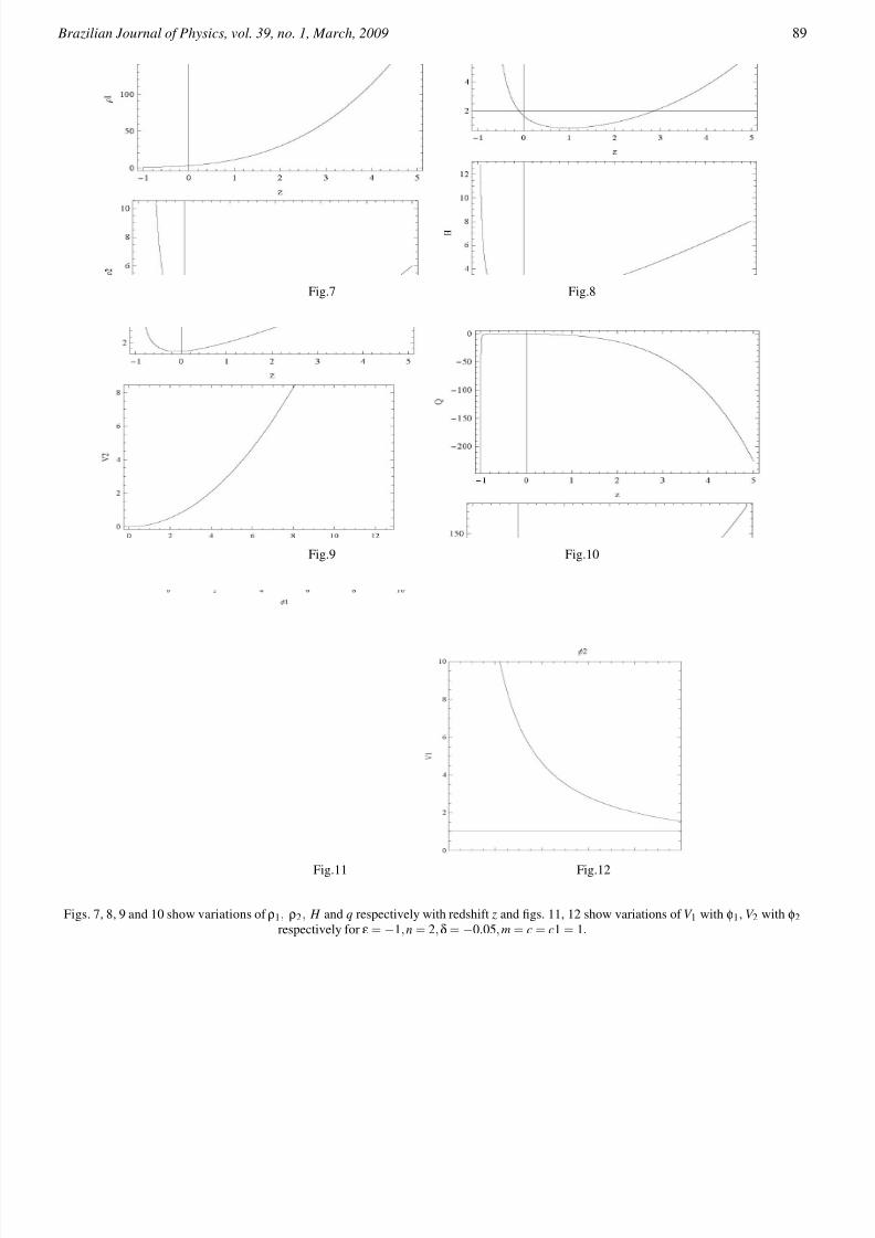
φ1, V 2 with φ2 respectively for scalar field model. Figs. 7 - 10show the variations ρ1, ρ2, H , Q with redshift z and figs. 11,

12 show the variations of V 1 with φ1, V 2 with φ2 respectively

for phantom model. For scalar field model ρ1, ρ2, H , Q

decrease with decreasing z but for phantom model ρ1, ρ2, H

decrease first and then increase with decreasing z and Q

decreases with decreasing z. The tachyonic field and scalar

field potentials always decrease, but phantom field potential

always increases. For scalar field model (ε = +1) and phan-

tom phantom field model (ε = −1), δ may be negative due topositivity of φ2

2. So from equations (11) and (12), it may be

concluded that the energy for scalar field will be transferred to

tachyonic field the energy for phantom field will be transferred

to tachyonic field. In both the cases, the interaction term




Fig.7 Fig.8

Fig.9 Fig.10

Fig.11 Fig.12

Figs. 7, 8, 9 and 10 show variations of ρ1, ρ2, H and q respectively with redshift z and figs. 11, 12 show variations of V 1 with φ1, V 2 with φ2

respectively for ε =−1,n = 2,δ =−0.05,m = c = c1 = 1.



90 Surajit Chattopadhyay and Ujjal Debnath

Fig.13 Fig.14

Fig.15 Fig.16

Figs. 13, 14 show the variations of V 1 with φ1, V 2 with φ2 respectively for ε = +1,n = 2,δ = 0,m = c = c1 = 1 and Figs. 15, 16 show the

variations of V 1 with φ1, V 2 with φ2 respectively for ε =−1,n = 2,δ = 0,m = c = c1 = 1.

Acknowledgement

The authors wish to acknowledge the warm hospitality pro-

vided by IUCAA, Pune, India, where part of the work was

carried out. One of the authors (UD) is thankful to UGC,

Govt. of India for providing research project grant (No. 32-

157/2006(SR)).

[1] N. A. Bachall, J. P. Ostriker, S. Perlmutter and P. J. Steinhardt,

Science 284 1481 (1999).

[2] S. J. Perlmutter et al, Astrophys. J. 517 565 (1999).

[3] V. Sahni and A. A. Starobinsky, Int. J. Mod. Phys. A 9 373

(2000).

[4] P. J. E. Peebles and B. Ratra, Rev. Mod. Phys. 75 559 (2003).

[5] T. Padmanabhan, Phys. Rept. 380 235 (2003).

[6] E. J. Copeland, M. Sami, S. Tsujikawa, Int. J. Mod. Phys. D 15

1753 (2006).

[7] I. Maor and R. Brustein, Phys. Rev. D 67 103508 (2003); V. H.

Cardenas and S. D. Campo, Phys. Rev. D 69 083508 (2004); P.G.

Ferreira and M. Joyce, Phys. Rev. D 58 023503 (1998).

[8] A. Melchiorri, L. Mersini, C. J. Odmann and M. Trodden, Phys.

Rev. D 68 043509 (2003).

[9] A. Feinstein, Phys. Rev. D 66 063511 (2002).

[10] M. Sami, Mod. Phys. Lett. A 18 691 (2003).

[11] A. Sen, JHEP 0204 048 (2002).

[12] A. Sen, JHEP 0207 065 (2002).

[13] G. W. Gibbons, Phys. Lett. B 537 1 (2002).

[14] M. Sami, P. Chingangbam and T. Qureshi, Phys. Rev. D 66

043530 (2002).

[15] M. Fairbairn and M.H.G. Tytgat, Phys. Lett. B 546 1 (2002).

[16] T. Padmanabhan, Phys. Rev. D 66 021301 (2002).

[17] J. S. Bagla, H. K. Jassal and T. Padmanabhan, Phys. Rev. D 67

063504 (2003); E. J. Copeland, M. R. Garousi, M. Sami and S.

Tsujikawa, Phys. Rev D 71 043003 (2005); G. Calcagni and A.

R. Liddle, Phys. Rev. D 74 043528 (2006).

[18] M. Sami, P. Chingangbam and T. Qureshi, Pramana 62 765




(2004).

[19] L. Parker and A. Raval, Phys. Rev. D 60 063512 (1999); D. Po-

larski and A. A. Starobinsky, Phys. Rev. Lett. 85 2236 (2000); R.

R. Caldwell, Phys. Lett. B 545 23 (2002).

[20] M. S. Berger, H. Shojaei, Phys. Rev. D 74 043530 (2006).

[21] R. Herrera, D. Pavon, W. Zimdahl, Gen. Rel. Grav. 36 2161

(2004); R. -G. Cai and A. Wang, JCAP 0503 002 (2005); Z.-

K. Guo, R.-G. Cai and Y.-Z. Zhang, JCAP 0505 002 (2005); T.

Gonzalez and I. Quiros, gr-qc /0707.2089.

[22] S. Chattopadhyay, U. Debnath and G. Chattopadhyay, Astro-

phys. Space Sci. 314 41 (2008).

surajit chattopadhyay and ujjal debnath- tachyonic field interacting with scalar (phantom) field

Documents