surface chemistry tutorial - noble innovations · careful attention is paid to the averall mass...

Solved with COMSOL Multiphysics 4.2

© 2 0 1 1 C O M S O L 1 | S U R F A C E C H E M I S T R Y TU T O R I A L

S u r f a c e Ch em i s t r y T u t o r i a lIntroduction

Surface chemistry is often the most important and most overlooked aspect of reacting flow modeling. Surface rate expressions can be hard to find or not even exist at all. Often it is preferable to use sticking coefficients to describe surface reactions because they can be estimated intuitively.

Model Definition

The tutorial model simulates outgassing from a wafer during a chemical vapor deposition (CVD) process. Careful attention is paid to the averall mass balance in the system and the difference between the mass averaged velocity and diffusion velocity is explored. The geometry and operating principle for the model is shown in Figure 1. Initially the closed container is full of 99.9% silicon hydride and 0.1% hydrogen (measured by molar content).

Wafer (red)

SiH4 converted to Si and H2 H2 outgassing

Figure 1: Geometry and basic operating principle for the surface chemistry tutorial model.

A surface reaction begins to occur on the wafer which consumes the silicon hydride, releases hydrogen into the domain, alters the composition of the absorbed species on


2 | S U R F A C E C H E M I S T R Y TU T O R I A L © 2 0 1 1 C O M S O L

the wafer surface and deposits bulk silicon. The following reactions are considered on the surface of the wafer:

The (s) here denotes “surface species” which means that the species only exists on the surfaces where the reaction is ocurring. To indicate that a species is bulk, append (b) to the end of the species. Since bulk species cannot participate in surface reactions, they must only be products and not reactants in a surface reaction. The net result of these two competing reactions is SiH4=>Si(b)+2H2, which means it is expected that the silane is replaced by hydrogen inside the reactor, and layers of silicon deposited on the wafer surface.

M O D E L E Q U A T I O N S - S U R F A C E R E A C T I O N S A N D S U R F A C E S P E C I E S

The surface reaction rate for reaction i is given by:

(1)

where the rate constant, kf is given by:

(2)

and ck is the concentration of species k which may be a volumetric or surface species, m is the reaction order minus 1, T is the surface temperature, R is the gas constant and Mn is the mean molecular weight of the gas mixture. Gamma_i is the dimensionless sticking coefficient. For the surface species the following equations are solved:

(3)

where is the surface site concentration (mol/m2), qi is the reaction rate for reaction i (mol/m2), i is the change in site occupancy number for reaction i (dimensionless).

TABLE 0-1: SURFACE REACTIONS CONSIDERED

REACTION STICKING COEFFICIENT

SiH4+2Si(s)=>Si(b)+2SiH(s)+H2 1E-4

SiH(s)=>Si(s)+0.5H2 1E-4

qi kf i ckkif

k 1=

K

=

kf ii

1 i 2–-------------------- 1

totm

------------------- 14--- 8RT

Mn------------=

tdd qi i

i 1=

N

=



(4)

where tot is the total surface site concentration (mol/m2), Zk is the site fraction (dimensionless) and R is the surface rate expression (mol/m2).

For the bulk surface species, the following equation is solved for the deposition height:

(5)

where h is the total growth height (m), M is the molecular weight (kg/mol) and is the density of the bulk species (kg/m3).

D O M A I N E Q U A T I O N S

Inside the domain, the Navier-Stokes equations are solved for the fluid velocity. The mass fraction of hydrogen is computed by solving:

(6)

where w is the mass fraction of hydrogen. For detailed information on the transport of the non-electron species see Theory for the Heavy Species Transport Interface in the Plasma Module User’s Guide. The mass fraction of silane is not directly computed. It’s value comes from the fact that the sum of the mass fractions must equal one. The gas temperature is computed by solving the energy equation.

B O U N D A R Y C O N D I T I O N S

Fluid FlowThe following boundary conditions are used. The mass averaged velocity is constrained using:

(7)

where Mf is the inward (or outward in this example) mass flux which is defined, from the surface chemistry as:

(8)

td

dZk Rtot----------=

tddh RMw--------------–=

tw u w+ j=

uMf-------n–=

Mf Mks·kk 1=

Kg

=



where sk is the surface rate expression for each species which comes from summing the surface reaction rates multiplied by their stoichiometric coefficients over all surface reactions:

(9)

Hydrogen Mass FractionThe flux of hydrogen at the surface of the wafer comes from the surface reactions:

(10)

Energy EquationFor the energy equation, the following boundary condition is used:

(11)

where hi is the molar enthalpy change due to reaction i.

Results and Discussion

The y-component of the mass averaged velocity is plotted in Figure 2. The mass averaged velocity is negative at the surface of the wafer. This means that overall, mass is leaving the system. This is to be expected since silane is being consumed, which has

s·k kiqii 1=

I

=

n j Mksk=

n T qihii 1=

I

=



a molecular weight of 0.032 kg/mol and replacing it with hydrogen, which has a lower molecular weight of 0.002 kg/mol.

Figure 2: Plot of the mass averaged velocity field after 5 seconds.

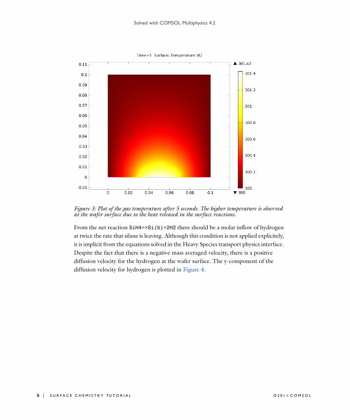
The surface reactions begin to consume the silane which results in concentration gradients within the reactor. The outward mass flux at the wafer surface leads to a mass averaged velocity everywhere inside the reactor. The combination of concentration gradients and convection due to the mass averaged velocity tends to draw silane to wards the wafer. The first surface reaction is exothermic while the second surface reaction is ednothermic. The amount of heat released by the exothermic reaction dominates, so the temperature begins to increase. The temperature is plotted in Figure 3 and is highest on the wafer surface.



Figure 3: Plot of the gas temperature after 5 seconds. The higher temperature is observed at the wafer surface due to the heat released in the surface reactions.

From the net reaction SiH4=>Si(b)+2H2 there should be a molar inflow of hydrogen at twice the rate that silane is leaving. Although this condition is not applied explicitely, it is implicit from the equations solved in the Heavy Species transport physics interface. Despite the fact that there is a negative mass averaged velocity, there is a positive diffusion velocity for the hydrogen at the wafer surface. The y-component of the diffusion velocity for hydrogen is plotted in Figure 4.



Figure 4: Plot of the y-component of the diffusion velocity for hydrogen after 5 seconds. Even though the mass averaged velocity is negative, the diffusion velocity is positive indicating an inflow of hydrogen and a net outflow of total mass.

Figure 5 plots the integrated pressure in the reactor divided by the initial average pressure in the reactor. Once the problem reaches steady state the average pressure in the reactor has increased by a factor of 2. This is expected since every mole of silane is being replaced by two moles of hydrogen. The silane in the reactor is completely consumed after around 200 seconds.



Figure 5: Plot of the ratio of the average pressure at time t divided by the average initial pressure.

In Figure 6 the total mass initially present in the reactor divided by the total mass in the reactor is plotted. The total mass in the reactor drops by a factor of 8, which is expected since the silane with molecular mass 0.032 kg/mol is replaced with two moles of hydrogen which has a molecular weight of 2·0.002=0.004 kg/mol.



Figure 6: Plot of the total mass in the reactor at t = 0 divided by the total mass at t = t.

Another way of verifying the correctness of the model is to compare the mass lost inside the reactor to the mass accumulated on the wafer surface. The two quantities should be equal. The total gain in mass from surface and bulk species is compared to the total loss in mass from the reactor in Figure 7. The two curves agree very well indicating that the total mass in the entire system is conserved.



Figure 7: Plot of the total mass lost in the domain (blue) and the total mass gained due to Silicon deposition on the wafer surface (green).

The ultimate goal of most CVD models is to determine the total growth height and growth rate on the surface of the wafer. The total growth height is plotted in Figure 8 and saturates at about 159 Angstroms. The total growth rate saturates because all the silane in the reactor is consumed after around 200 seconds. The accumulated growth height is also very uniform across the surface of the wafer.



Figure 8: Plot of the growth height (surface and z-axis) vs. the wafer arc length (x-axis) and time (y-axis). The final height of deposited silicon is 158 Å.

Reference

1. R.J. Kee, M.E. Coltrin, and P. Glarborg, Chemically Reacting Flow Theory and Practice, Wiley, 2003.

Model Library path: Plasma_Module/CVD_Models/surface_chemistry_tutorial

Modeling Instructions

In the Model Builder window’s toolbar, click the Show button and select Stabilization in the menu.

In the Model Builder window’s toolbar, click the Show button and select Discretization in the menu.



In the Model Builder window’s toolbar, click the Expand sections button and select Stabilization in the menu.

In the Model Builder window’s toolbar, click the Expand sections button and select Discretization in the menu.

M O D E L W I Z A R D

1 Go to the Model Wizard window.

2 Click the 2D button.

3 Click Next.

4 In the Add physics tree, select Plasma>Heavy Species Transport (hs).

5 Click Add Selected.

6 In the Add physics tree, select Fluid Flow>Single-Phase Flow>Laminar Flow (spf).


8 In the Add physics tree, select Heat Transfer>Heat Transfer in Fluids (ht).


10 Click Next.

11 In the Studies tree, select Preset Studies for Selected Physics>Time Dependent.

12 Click Finish.

G E O M E T R Y 1

Square 11 In the Model Builder window, right-click Model 1>Geometry 1 and choose Square.

2 Go to the Settings window for Square.

3 Locate the Size section. In the Side length edit field, type 0.1.

4 Click the Build All button.

Polygon 11 In the Model Builder window, right-click Geometry 1 and choose Polygon.

2 Go to the Settings window for Polygon.

3 Locate the Coordinates section. In the x edit field, type 0.03 0.07.

4 In the y edit field, type 0 0.



D E F I N I T I O N S

Variables 11 In the Model Builder window, right-click Model 1>Definitions and choose Variables.

2 Go to the Settings window for Variables.

3 Locate the Variables section. In the Variables table, enter the following settings:

Integration 11 In the Model Builder window, right-click Definitions and choose Model

Couplings>Integration.

2 Select Domain 1 only.

Integration 21 In the Model Builder window, right-click Definitions and choose Model

Couplings>Integration.

2 Go to the Settings window for Integration.

3 Locate the Source Selection section. From the Geometric entity level list, select Boundary.

4 Select Boundary 4 only.

NAME EXPRESSION DESCRIPTION

mass_domain at(0,intop1(hs.rho))-intop1(hs.rho)

Mass change in the domain

mass_bulk intop2(h_Si_bulk*2329[kg/m^3])

Total mass of bulk species

mass_Si_surf

intop2(Zk_Si_surf*gamman_Si_surf/hs.sigmak_Si_surf*0.028[kg/mol])

Total mass of Si surface species

mass_SiH_surf

intop2(Zk_SiH_surf*gamman_SiH_surf/hs.sigmak_SiH_surf*0.029[kg/mol])

Total mass of SiH surface species

dmass_Si_surf

mass_Si_surf-at(0,mass_Si_surf)

Total mass minus initial mass of Si surface species

dmass_SiH_surf

mass_SiH_surf-at(0,mass_SiH_surf)

Total mass minus initial mass of SiH surface species

mass_surf dmass_Si_surf+dmass_SiH_surf

Total mass minus initial mass of all surface species



H E A V Y S P E C I E S TR A N S P O R T

1 In the Model Builder window, click Model 1>Heavy Species Transport.

2 Go to the Settings window for Heavy Species Transport.

3 Locate the Transport Settings section. Select the Calculate thermodynamic properties check box.

4 Clear the Migration in electric field check box.

5 Select the Convection check box.

Surface Reaction 11 Right-click Model 1>Heavy Species Transport and choose Surface Reaction.

2 Go to the Settings window for Surface Reaction.

3 Locate the Reaction Formula section. In the Formula edit field, type SiH4+2Si(s)=>Si(b)+2SiH(s)+H2.


5 Locate the Kinetics Expressions section. In the f edit field, type 1E-4.

Surface Reaction 21 In the Model Builder window, right-click Heavy Species Transport and choose Surface

Reaction.

2 Go to the Settings window for Surface Reaction.

3 Locate the Reaction Formula section. In the Formula edit field, type SiH(s)=>Si(s)+0.5H2.


5 Locate the Kinetics Expressions section. In the f edit field, type 1E-4.

Species: SiH41 In the Model Builder window, click Species: SiH4.

2 Go to the Settings window for Species.

3 Locate the Species Formula section. Select the From mass constraint check box.

4 Locate the General Parameters section. From the Preset species data list, select SiH4.

Species: H21 In the Model Builder window, click Species: H2.

2 Go to the Settings window for Species.

3 Locate the General Parameters section. From the Preset species data list, select H2.

4 In the x0 edit field, type 1E-3.



Species: Si(s)1 In the Model Builder window, click Species: Si(s).

2 Go to the Settings window for Surface Species.

3 Locate the General Parameters section. From the Preset species data list, select Si.

4 Locate the Surface Species Parameters section. In the Zk,0 edit field, type 0.995.

Species: Si(b)1 In the Model Builder window, click Species: Si(b).


3 Locate the General Parameters section. From the Preset species data list, select Si.

Species: SiH(s)1 In the Model Builder window, click Species: SiH(s).


3 Locate the General Parameters section. From the Preset species data list, select SiH.

4 Locate the Surface Species Parameters section. In the Zk,0 edit field, type 0.005.

Convection and Diffusion1 In the Model Builder window, click Convection and Diffusion.

2 Go to the Settings window for Convection and Diffusion.

3 Locate the Model Inputs section. From the u list, select Velocity field (spf/fp1).

4 From the T list, select Temperature (ht/fluid1).

5 From the p list, select Pressure (spf/fp1).

6 Clear the Reference pressure check box.

L A M I N A R F L O W

Fluid Properties 11 In the Model Builder window, expand the Model 1>Laminar Flow node, then click Fluid

Properties 1.

2 Go to the Settings window for Fluid Properties.

3 Locate the Fluid Properties section. From the list, select Density (hs/cdm1).

4 From the list, select Dynamic viscosity (hs/cdm1).

Initial Values 11 In the Model Builder window, click Initial Values 1.

2 Go to the Settings window for Initial Values.



3 Locate the Initial Values section. In the p edit field, type 13.3.

4 In the Model Builder window, click Laminar Flow.

5 Go to the Settings window for Laminar Flow.

6 Locate the Consistent Stabilization section. Clear the Crosswind diffusion check box.

7 Click to expand the Discretization section.

8 From the Discretization of fluids list, select P2 + P1.

Inlet 11 In the Model Builder window, right-click Laminar Flow and choose Inlet.


3 Go to the Settings window for Inlet.

4 Locate the Boundary Condition section. From the Boundary condition list, select Mass flow.

5 Locate the Mass Flow Rate section. From the Mass flow type list, select Pointwise mass flux.

6 From the Mf list, select Inward mass flux (hs/hs).

H E A T TR A N S F E R

Heat Transfer in Fluids 11 In the Model Builder window, expand the Model 1>Heat Transfer node, then click Heat

Transfer in Fluids 1.

2 Go to the Settings window for Heat Transfer in Fluids.

3 Locate the Model Inputs section. From the p list, select Pressure (spf/fp1).

4 Clear the Reference pressure check box.

5 From the u list, select Velocity field (spf/fp1).

6 Locate the Heat Conduction section. From the k list, select Thermal conductivity (hs/cdm1).

7 Locate the Thermodynamics section. From the Fluid type list, select Ideal gas.

8 From the Gas constant type list, select Mean molar mass.

9 From the Mn list, select Mean molar mass (hs/cdm1).

10 From the Cp list, select Mass-averaged mixture specific heat (hs/cdm1).

Temperature 11 In the Model Builder window, right-click Heat Transfer and choose Temperature.



2 Select Boundaries 1, 3, and 6 only.

3 Go to the Settings window for Temperature.

4 Locate the Temperature section. In the T0 edit field, type 300.

Initial Values 11 In the Model Builder window, click Initial Values 1.

2 Go to the Settings window for Initial Values.

3 Locate the Initial Values section. In the T edit field, type 300.

Reaction Heat Flux 11 In the Model Builder window, right-click Heat Transfer and choose Reaction Heat Flux.


3 Go to the Settings window for Reaction Heat Flux.

4 Locate the Reaction Heat Flux section. From the Qb list, select Total surface heat source of reaction (hs/hs).

M E S H 1

Size 11 In the Model Builder window, right-click Model 1>Mesh 1 and choose Size.

2 Go to the Settings window for Size.

3 Locate the Geometric Entity Selection section. From the Geometric entity level list, select Point.

4 Select Vertices 3 and 4 only.


6 Locate the Element Size section. From the Predefined list, select Extremely fine.

7 Click the Custom button.

8 Locate the Element Size Parameters section. Select the Maximum element size check box.

9 In the associated edit field, type 0.0002.

Edge 11 In the Model Builder window, right-click Mesh 1 and choose More Operations>Edge.


Size 11 Right-click Edge 1 and choose Size.




3 Locate the Element Size section. From the Predefined list, select Extremely fine.

Free Triangular 11 In the Model Builder window, right-click Mesh 1 and choose Free Triangular.

2 In the Settings window, click Build All.

S T U D Y 1

Step 1: Time Dependent1 In the Model Builder window, expand the Study 1 node, then click Step 1: Time

Dependent.

2 Go to the Settings window for Time Dependent.

3 Locate the Study Settings section. In the Times edit field, type range(0,5,300).

4 In the Model Builder window, right-click Study 1 and choose Show Default Solver.

5 Expand the Study 1>Solver Configurations node.

Solver 11 In the Model Builder window, expand the Study 1>Solver Configurations>Solver 1

node.

2 In the Model Builder window, click Time-Dependent Solver 1.

3 Go to the Settings window for Time-Dependent Solver.

4 Click to expand the Absolute Tolerance section.

5 From the Global method list, select Unscaled.

6 Click to expand the Time Stepping section.

7 In the Initial step edit field, type 0.001.

8 In the Model Builder window, right-click Study 1 and choose Compute.

R E S U L T S

Velocity (spf)1 Go to the Settings window for 2D Plot Group.

2 Locate the Data section. From the Time list, select 5.

3 In the Model Builder window, click Surface 1.

4 Go to the Settings window for Surface.

5 In the upper-right corner of the Expression section, click Replace Expression.



6 From the menu, choose Laminar Flow>Velocity field>Velocity field, y component (v).

7 Click the Plot button.

Temperature (ht)1 In the Model Builder window, click Results>Temperature (ht).

2 Go to the Settings window for 2D Plot Group.



2D Plot Group 61 In the Model Builder window, right-click Results and choose 2D Plot Group.



4 Right-click Results>2D Plot Group 6 and choose Surface.



7 From the menu, choose Diffusion velocity, y component (hs.Vdy_wH2).




3 Click to expand the Legend section.

4 From the Position list, select Lower right.

5 Right-click Results>1D Plot Group 7 and choose Global.

6 Go to the Settings window for Global.

7 Click to expand the Legends section.

8 Select the Expression check box.

9 Clear the Description check box.

10 Locate the y-Axis Data section. In the table, enter the following settings:


EXPRESSION UNIT DESCRIPTION

intop1(p)/at(0,intop1(p))

1 Average pressure divided by average intitial pressure












10 Locate the y-Axis Data section. In the table, enter the following settings:











10 Locate the y-Axis Data section. In the #-axis data table, enter the following settings:



at(0,intop1(hs.rho))/intop1(hs.rho)

1 Initial mass in the reactor divided by the mass in the reactor


mass_domain Total mass in the domain

mass_surf+mass_bulk Total mass of surface plus bulk species



Data Sets1 In the Model Builder window, right-click Results>Data Sets and choose Edge 2D.


3 In the Model Builder window, right-click Data Sets and choose Parametric Extrusion 1D.

2D Plot Group 101 Right-click Results and choose 2D Plot Group.


3 Locate the Data section. From the Data set list, select Parametric Extrusion 1D 1.

4 Right-click Results>2D Plot Group 10 and choose Surface.



7 From the menu, choose Heavy Species Transport>Displacement field (h_Si_bulk).

8 Locate the Expression section. From the Unit list, select Å.

9 Right-click Surface 1 and choose Height Expression.

10 In the Settings window, click Plot.

surface chemistry tutorial - noble innovations · careful attention is paid to the averall mass...

Documents