Surface Reconstruction from Scattered Point viaRBF Interpolation on GPU

Salvatore Cuomo∗, Ardelio Galletti†, Giulio Giunta†, Alfredo Starace†∗Department of Mathematics and Applications “R. Caccioppoli” University of Naples Federico II

c/o Universitario M.S. Angelo 80126 Naples Italyemail:salvatore.cuomo@unina.it

†Department of Applied Science. University of Naples “Parthenope”.Centro Direzionale, Isola C4 80143 Naples Italy

emails:ardelio.galletti,giulio.giunta@uniparthenope.it, alfredo.starace@gmail.com

Abstract—In this paper we describe a parallel implicit methodbased on radial basis functions (RBF) for surface reconstruction.The applicability of RBF methods is hindered by its computa-tional demand, that requires the solution of linear systems of sizeequal to the number of data points. Our reconstruction imple-mentation relies on parallel scientific libraries and is supportedfor massively multi-core architectures, namely Graphic ProcessorUnits (GPUs). The performance of the proposed method in termsof accuracy of the reconstruction and computing time shows thatthe RBF interpolant can be very effective for such problem.

I. INTRODUCTION

Many applications in engineering and science need to buildaccurate digital models of real-world objects defined in termsof point cloud data, i.e. a set of scattered points in 3D.Typical examples include the digitalization of manufacturedparts for quality control, statues and artifacts in archeologyand arts [10], human bodies for movies or video games, organsand anatomical parts for medical diagnostic [4] and elevationmodels for simulations and modeling [14]. Using modern 3Dscanners, it is possible to acquire point clouds containingmillions of points sampled from an object. The process ofbuilding a geometric model from such point clouds is usuallyreferred to as surface reconstruction.

There are several approaches to reconstruct surfaces from3D scattered datasets. Generally, the methods of surfacereconstruction fall into two categories [15]: Delaunay-basedmethods and volumetric and implicit based methods. Delaunaytriangulation is usually utilized to find the possible neighborsfor each point in all directions from all samples. Implicit sur-face modeling instead is most popular for describing complexshapes and complex editing operations. Among them, level setmethods [23], moving least square methods [9], variationalimplicit surfaces [20] and adaptively sampled distance field[8] are recent developments in this field. In this paper wefocus on the implicit surface method based on radial basisfunctions (RBFs). In the 1980’s, Franke [7] used radial basisfunctions to interpolate scattered point cloud firstly and provedthe accuracy and stability of the interpolation based on RBFs.Using this technique, an implicit surface is constructed bycalculating the weights of a set of radial basis functions whoselinear combination interpolates the given data points.

The RBF applicability is hindered by its computationaldemand, since these methods require the solution of a linearsystem of size equal to the number of data points and current3D data scanners allow acquisition of tens of millions pointsof an object surface.

High Performance Computing (HPC) is a natural solution toprovide the computational power required in such situations.In this paper we propose a method designed for a massivelymulti-core architecture, namely Graphics Processing Units(GPUs) [17]. Recently, GPUs have been effectively used toaccelerate the performance of applications in several scien-tific areas such as computational fluid dynamics, moleculardynamics, climate modeling [6]. For our knowledge, the mostefficient parallel algorithm for RBF interpolation is “PetRBF”[21]. PetRBF is a parallel algorithm for RBF interpolation thatexhibits O(N) complexity, requires O(N) storage, and scalesexcellently up to a thousand processes. Our main contributeis a deep re-engineering of PetRBF which constitutes a gen-eralization for scattered 3D data and an extension for GPUacceleration on heterogeneous clusters. We also focus on thesuitable choice of the algorithm parameters and present anoptimal strategy for synthetic, real or incomplete datasets.

In section II we deal mathematical Preliminaries, in sectionIII we describe the related works and the implementationstrategies. The section IV we report the numerical experimentsand finally we draw conclusions in section V.

II. PRELIMINARIES

In this section we recall the reconstruction based on im-plicit surface method and define the related RBF interpolationproblem.

A. Implicit Surface Reconstruction

Given a point cloud

X := (xi, yi, zi) ∈ R3, i = 1, . . . , N

coming from an unknown surfaceM, i.e. X ⊂M, the goal isto find another surface M∗ which is a reconstruction of M.In the implicit surface approach M is defined as the surfaceof all points (x, y, z) ∈ R3 that satisfy the implicit equation

f(x, y, z) = 0 (1)

arX

iv:1

305.

5179

v1 [

cs.D

C]

22

May

201

3

for an unknown function f . A way to approximate f is toimpose the interpolation conditions (1) on the point cloud X .However, the use of those interpolation conditions only leadsto the trivial solution given by the identically zero function,whose zero surface is R3. Therefore, the key for finding anapproximation of the function f is to use additional significantinterpolation conditions, i.e. on correspondence of off-surfacepoints (where f 6= 0). This involves a nontrivial interpolantPf , whose zero surface contains a meaningful surface M∗.This approach leads to a surface reconstruction method whichconsists of three main steps:

1) generation of off-surface points;2) interpolant model identification on the extended dataset;3) computation of the interpolation zero iso-surface.1) Generation of off-surface points:

A common practice, as suggested in [19], is to use the set ofsurface normals ni = (nxi , n

yi , n

zi ) to the surface M at points

xi = (xi, yi, zi). If these normals are not explicitly known,there are techniques and tools1 that to allow to estimate them.Given the oriented surface normals (ni and −ni), we generatethe extra off-surface points by marching a small distance δalong the normals. So, we obtain for each cloud data pointxi = (xi, yi, zi) two additional off-surface points. The firstlies “outside” the surface M and is given by

(xN+i, yN+i, zN+i) = xi + δni =

= (xi + δnxi , yi + δnyi , zi + δnzi );

the other point lies “inside” and is given by

(x2N+i, y2N+i, z2N+i) = xi − δni =

= (xi − δnxi , yi − δnyi , zi − δn

zi ).

The union of the sets X+δ = xN+1, . . . ,x2N, X−δ =

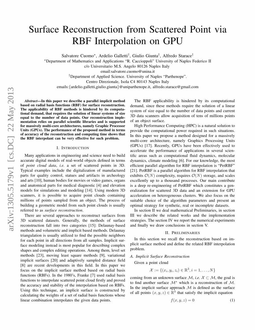
x2N+1, . . . ,x3N and X gives the overall set of points onwhich the interpolation conditions are assigned (see Fig. 1).The set X+

δ implicitly defines a surface M+δ which passes

Fig. 1. Extended interpolation data set. In black points from X , in bluepoints from X+

δ and in green points from X−δ

through its points. Analogously X−δ defines the surface M−δ .Those two surfaces can be considered respectively externaland internal to M. The value of δ represents a small stepsize whose specific magnitude may be rather critical for a

1package ply.tar.gz provided by Greg Turk, available athttp://www.cc.gatech.edu/projects/large models/ply.html

good surface reconstruction [3]. In particular, if δ is chosentoo large, this results in self intersectingM+

δ orM−δ auxiliarysurfaces. In our implementation we fix δ to 1% of the boundingbox of the data as suggested in [22].

2) Interpolant model identification on extended dataset:This step consists in determining a function Pf whose zerocontour interpolates the given point cloud data X and whoseiso-surface Pf = 1 and Pf = −1 interpolate X+

δ and X−δ ,respectively, i.e.

Pf (xi) =

0 i = 1, . . . , N1 i = N + 1, . . . , 2N−1 i = 2N + 1, . . . , 3N

The values of ±1 for the auxiliary data are assigned in anarbitrary way. Such choice does not affect the quality of theresults. In this discussion we are interested to the iso-surfacezeros of Pf .

3) Computation of the interpolation zero iso-surface:In order to evaluate the Pf zero iso-surface and visualizeit, we use a simple strategy which consists on evaluatingthe interpolant Pf on a dense grid of a bounding box.This approach leads to some undesired artifacts, since in thebounding box there are points that do not belong to M∗. Apossible way to overcome this drawback and display onlyM∗ consists in evaluating the interpolant only in a smallsurrounding volume of the surface M to reconstruct. Thisset is denoted as Mε

ext = x ∈ R3 : d(x,M) ≤ ε, whered(x,M) = inf

y∈M‖y − x‖. For a small enough value of ε it

holdsM∗ ≈Mε

ext ∩ S0.

where S0 is the zero iso-surface of Pf .

B. RBF interpolation

Given a set of N distinct points (xj , yj), j = 1, . . . , N ,where xj ∈ Rs and yj ∈ R, the scattered data interpolationproblem is to find an interpolant function Pf such that:

Pf (xj) = yj , j = 1, . . . , N. (2)

In the univariate setting, the interpolant Pf is usually chosenin suitable spaces of functions. A common approach assumesthat the function Pf is a linear combination of certain basisfunction Bj , i.e.

Pf (x) =

N∑j=1

cjBj(x). (3)

In the multivariate setting (xj ∈ Rs, s > 1), however, theproblem is much more complex. As stated by the Mairhuber-Curtis theorem [5], [11], in order to have a well-posed multi-variate scattered data interpolation problem it is not possibleto fix in advance the basis B1, . . . , BN. Instead the basismust depend on the data location.

In order to obtain data dependent approximation space, assuggested by the Mairhuber-Curtis theorem, the RBF interpo-lation uses radial functions:

Bj ≡ Φj = ϕ(‖x− xj‖).

The points xj to which the basic function ϕ is shifted areusually referred as centers. While there may be circumstancesthat suggest to choose these centers different from the datasites one generally picks the centers to coincide with the datasites.

The interpolation problem consists of two subproblems:finding the interpolant Pf and evaluating it on an assigned setof points. The coefficients cj in (3) are obtained by imposingthe interpolation conditions (2)

Pf (xi) =

N∑j=1

cjϕ(‖xi − xj‖) = yi, i = 1, . . . , N.

This leads to solve a linear system of equations (4).Given a set of M points ξ = ξ1, ξ2, . . . , ξM the evaluation

of the interpolant Pf on ξ can be computed with a matrixvector product (5)

The RBF interpolant determination consists to solve a linearsystem of equations Ax = b. In order to have a well-posedproblem the matrix A must be non-singular. Unfortunately noone has yet succeeded in characterizing the class of all basicfunction ϕ that generates a non-singular matrix for arbitraryset X = x1, . . . , xN of distinct data sites. The situationis however much better with positive definite matrices. Animportant property of positive definite matrices is that all theireigenvalues are positive, and therefore a positive definite ma-trix is non-singular. Popular radial basis function Φ, that giverise to positive definite interpolation matrices, are summarizedin Table II-B, we focused our work (as [21]) on the Gaussianfunction taking advantage of its property as described in §3.

III. PARALLEL SURFACE RECONSTRUCTION

A brief description of the overall surface reconstructionalgorithm is listed below:

Algorithm 1 Surface ReconstructionRequirements:point cloud X, surface normals ni,evaluation grid ξ

1: compute extended data set:Xext = X

⋃X+δ

⋃X−δ by using ni;

2: find the interpolant Pf on Xext;3: evaluate Pf on ξ;4: render the surface;

The steps 1 and 2 have been already discussed in §2.1;the step 3 requires a matrix vector multiplication as describedin §2.2 and the final step can be simply accomplished usingthe MATLAB software with the command isosurface orother specific tool for the rendering. The most computationalexpensive step is the second one, which requires the solutionof a system of 3N linear equation, where N is the initial pointcloud size, as described in §2.2. In the following section wedescribe the approach used to handle this problem.

A. Adopted solution

Handling problems with large numbers of data points, as inour case for surface reconstruction from clouds of millionsof points, the large amount of memory usage can becomea problem. As the problem size grows, parallelization ondistributed memory architectures becomes necessary. We adoptthe idea behind Domain Decomposition Methods (DDM)that is to divide the considered domain into a number ofsubdomains and then try to solve the original problem asa series of subproblems that interact through the interfaces.Let consider the domain Ω containing the point cloud; theadopted domain decomposition method divides the domainΩ in overlapping sub-domains Ωi. The corresponding emptyintersection portions of subdomains are denoted with Ωi, asshown in the example in Fig. 2. The solution of the linear

Fig. 2. Illustration of the Domain Decompostion Method.

system Ax = b on the whole domain can be obtained bysequentially solving, in the individual overlapping subdomainsΩi, the linear sub-system AixΩi = bΩi , where Ai, xΩi and bΩiare the sub-elements corresponding to domain Ωi for A, x, andb respectively. When each subdomain is solved individuallyand the solution of the entire domain is updated simultaneouslyat the end of each iteration step, the method is called additiveSchwarz method. Moreover, when the values x outside ofthe subdomain Ωi are discarded after the calculation of eachsubdomain Ωi, it is called restricted additive Schwarz method(RASM). The RASM is known to converge faster than theadditive Schwarz method and requires less communication inparallel calculations. Furthermore solving smaller systems ofequations has the same effect as a preconditioner, and then itcan be used in combination with any iterative method like theKrylov subspace methods. In this work we use the GeneralizedMinimum Residual (GMRES).

Using basis functions with negligible global effects, thematrix A can be considered to have a finite bandwidth. Inthis case, the calculation of the matrix-vector multiplication,which is the predominant operation of the iterative solver, canbe done somewhat locally. Using the Gaussian function as thebasic function the matrix A has the following elements:

Aij =1√2πσ

exp

(−‖xi − xj‖2

2σ2

). (6)

ϕ(‖x1 − x1‖) ϕ(‖x1 − x2‖) · · · ϕ(‖x1 − xN‖)ϕ(‖x2 − x1‖) ϕ(‖x2 − x2‖) · · · ϕ(‖x2 − xN‖)

......

. . ....

ϕ(‖xN − x1‖) ϕ(‖xN − x2‖) · · · ϕ(‖xN − xN‖)

︸ ︷︷ ︸

A

·

c1c2...cN

︸ ︷︷ ︸

x

=

y1

y2

...yN

︸ ︷︷ ︸

b

(4)

Pf (ξ1)Pf (ξ2)

...Pf (ξM )

=

ϕ(‖ξ1 − x1‖) ϕ(‖ξ1 − x2‖) · · · ϕ(‖ξ1 − xN‖)ϕ(‖ξ2 − x1‖) ϕ(‖ξ2 − x2‖) · · · ϕ(‖ξ2 − xN‖)

......

. . ....

ϕ(‖ξM − x1‖) ϕ(‖ξM − x2‖) · · · ϕ(‖ξM − xN‖)

·

c1c2...cN

(5)

TABLE IEXAMPLES OF RADIAL BASIS FUNCTIONS.

RBF Φ

Poisson radial functionJs/2−1(‖x−xj‖)

‖x− xj‖s/2−1s ≥ 2

Inverse Multiquadric (1 + ‖x− xj‖2)−β β > s2

Matern functionKα(‖x− xj‖)‖x− xj‖α

2β−1Γ(β)α = β − s

2> 0

Whittaker function∫ +∞0 (1− ‖x− xj‖)k−1

+ tαe−βtdt k = 2, 3, . . . , α = 0, 1, . . .

Gaussian function1

√2πσ

e−‖x−xj‖

2

2σ2 σ > 0

In this way, since the Gaussian function decays rapidly, theelements of matrix A corresponding to the interaction ofdistant points can be neglected. This sparsity of A dependson the relative size of the calculation domain compared to thestandard deviation, σ, of the Gaussian function. If σ is keptconstant while the size of the calculation domain is increasedalong with N , the calculation load will scale as O(N). Thecommunication required to perform Axi is also limited to aconstant number of elements in the vicinity. Therefore, theRASM becomes an extremely parallel algorithm with mini-mum communication for the surface reconstruction problemsthat have a domain size of hundreds (or even thousands) ofsigmas.

B. Implementation details

The algorithm implementation has been realized usingthe Portable, Extensible Toolkit for Scientific Computation(PETSc) [1]. PETSc is a scalable solver library developedat Argonne National Laboratory. All vectors and matricescan be distributed by PETSc and each process stores only alocal portion. This transparent management of PETSc allowsusers to develop scalable parallel code (almost) as serial code.In particular this is done by using the Vec PETSc objectfor vectors x and b. To handle the overlapping and non-overlapping subdomain the index sets (IS) were used. ThePETSc IS object is a global index that is used to definethe elements in each subdomain and is distributed among theprocesses in the same way as the vectors. The interpolationmatrix has entries which depends only from the vector x andthe Gaussian (eq. 6). For this reason it is possible to use theMatShell object which allow to make operations on the

matrix without actually storing the matrix. All calculation ofinner products, norms, and scalar multiplications are done bycalling PETSc routines and the linear system solution is finallycalculated with KSPSolve.

C. GPU implementation

GPU support has recently been added to PETSc to exploitthe performance of GPUs, these chips are highly optimized forgraphics-related operations. We use the CUDA framework thatgreatly simplifies the programming model for GPUs. The GPUimplementation of PETSc also uses some of those libraries.Instead of writing completely new CUDA code, PETSc usesthe open source libraries CUSP [13] e Thrust [18]. Thisallows transparent utilization of the GPU without changingthe existing source code of PETSc.

A new GPU specific Vector and Matrix classes calledVecCUSP and MatCUSP has been implemented in PETSc.The classes use CUBLAS, CUSP, as well as Thrust libraryroutines to perform matrix and vector operations on the GPU.The idea behind these libraries is to use already developed,fine tuned CUDA implementations with PETSc instead ofdeveloping new ones. The PETSc implementation acts asan interface between PETSc data structures and the externalCUDA libraries Thrust and CUSP.

Using the VecSetType() and MatSetType() PETScroutines, users can switch to the GPU version of the applica-tion simply using the command line parameters -vec_typecusp and -mat_type aijcusp. Cusp natively supportsseveral sparse matrix formats:• Coordinate list (COO)• Compressed Sparse Row (CSR)

• Diagonal (DIA)• ELLPACK (ELL)• Hybrid (HYB)

This feature is still in development in PETSc, howeverit can be used specifying --download-txpetscgpu--with-txpetscgpu=1 in the configuration and compila-tion phase of PETSc. After that it is possible for the applicationto switch between the sparse matrix formats with the commandline option-mat_cusp_storage_format <format>.

A simple GPU implementation can be obtained by passingto the MatShell a pointer to a function that call a CUDAkernel that execute the operations on the Matrix. A betteridea is to use the GPU version of PETSc objects wheneverpossible, in order to accelerate all the available operation,and not only those on the matrix. To this end there is theneed of building the matrices object. The Matrix for the inter-polant determination (step 2) can be easily constructed usingthe algorithm reported in Algorithm 2. For the interpolantevaluation (step 3) instead the only required operation is thematrix vector multiplication. For this reason the constructionof the matrix and the following matrix-vector multiplicationdone directly by PETSc using CUSP is less efficient than acustom matrix-vector multiplication CUDA kernel (Algorithm3) that consider the well known structure of the matrix (eq. 6)without the need of building the Matrix.

Algorithm 2 Interpolation matrix construction Pseudo-codealgorithm

1: for each subdomain Ωi do2: for each point xi in the subdomain Ωi do3: for each point xj in the truncation area of Ωi do

4: Set Aij = 1√2πσ

exp

(−‖xi − xj‖2

2σ2

)5: end for6: end for7: end for

IV. EXPERIMENTAL RESULTS

In this section we present some results of our methodfor surface reconstruction. The results presented here werecomputed using a system equipped with an Intel Core i7-940CPU (2,93 GHz, 8M Cache). The middleware framework isOS Linux kernel 2.6.32-28 and PETSc developer version 3.3.

Tests has been conducted to investigate the impact of theparameter σ on the quality of the reconstruction. As showedin §3.2 our method is highly efficient for small value of σcompared to the domain size. However, besides efficiency, thequality of the result also depends strongly on the value ofσ. This is because the accuracy of the interpolation modeldepends strongly on the ratio between the density of the pointcloud and σ.

In [21] experiments are carried out only on equally-spacedlattice point distributions. In this particular case they used asa measure for the density the spacing h between the points,

Algorithm 3 CUDA code of RBF evaluation algorithm1: __shared__ float sharedXi[BLOCK_SIZE];2: __shared__ float sharedGi[BLOCK_SIZE];3: int bx = blockIdx.x;4: int tx = threadIdx.x;5: int i = blockIdx.x * BLOCK_SIZE +threadIdx.x;

6: float pf = 0;7: float coeff = 0.5f/(sigma*sigma);8: for (unsigned int m = 0; m <(col-1)/BLOCK_SIZE+1; m++)

9: sharedXi[tx] = Xi[m*BLOCK_SIZE + tx];10: __syncthreads();11: for (unsigned int k = 0; k <

BLOCK_SIZE; k++) 12: dx = Xj[i]-sharedXi[k];13: pf += sharedGi[k]*exp(-(dx*dx)*coeff;14: Pf[i] = pf/M_PI*coef;

discovering that a good choice for σ, in term of performanceand accuracy, is the one that satisfy the ratio h/σ ≈ 1.

For widely scattered data, as in the case of points cloudfor surface reconstruction, there are more appropriate densitymeasure available. The first is the so-called separation distancedefined as

qX =1

2mini6=j‖xi − xj‖2. (7)

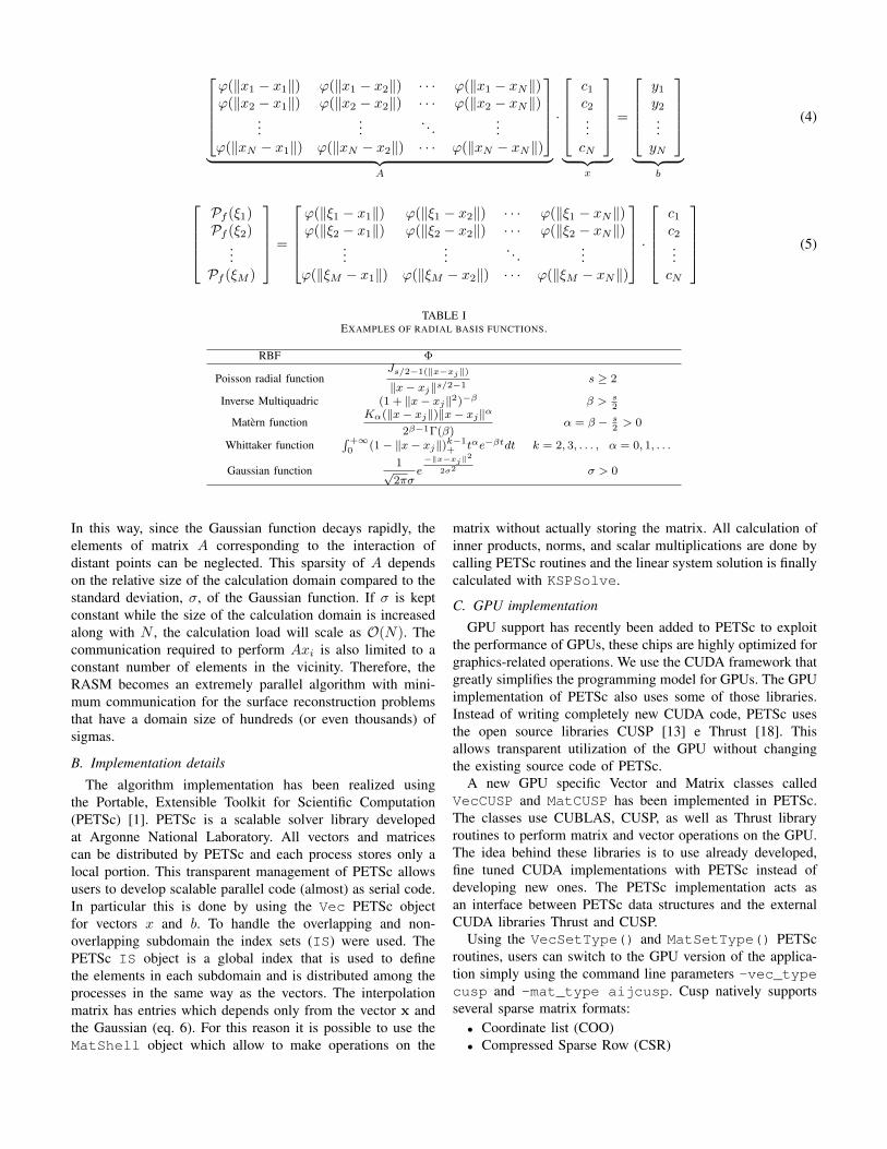
As shown in Fig. 3, qX geometrically represents the radius ofthe largest (hyper)sphere that can be drawn around each pointin such a way that no (hyper)sphere intersects the others, whichis why it is also sometimes called packing radius. Anothermeasure, usually used in approximation theory, is the so-calledfill distance:

hX ,Ω = supx∈Ω

minxj∈X

‖x− xj‖2. (8)

It indicates how well the set X fill the domain Ω. A geometricinterpretation of the fill distance is given by the radius of thebiggest empty (hyper)sphere that can be placed among thedata locations in Ω (see Fig. 3), for this reason it sometimesis also used as synonym the term covering radius. Hence forscattered data, using (7) and (8), the heuristic “optimal” ratioh/σ ≈ 1 assumes the following expressions:

σ ≈ 2qX (9)

andσ ≈ hX ,Ω

√2. (10)

A. Tests on synthetic dataset

We first conduct some experiment on a synthetic dataset.We choose as surface a sphere, whose geometry is well know,and on which it is possible to calculate (7) and (8). In orderto perform a consistent test with real dataset, we use a widelyscattered point cloud reported in Fig. 4.

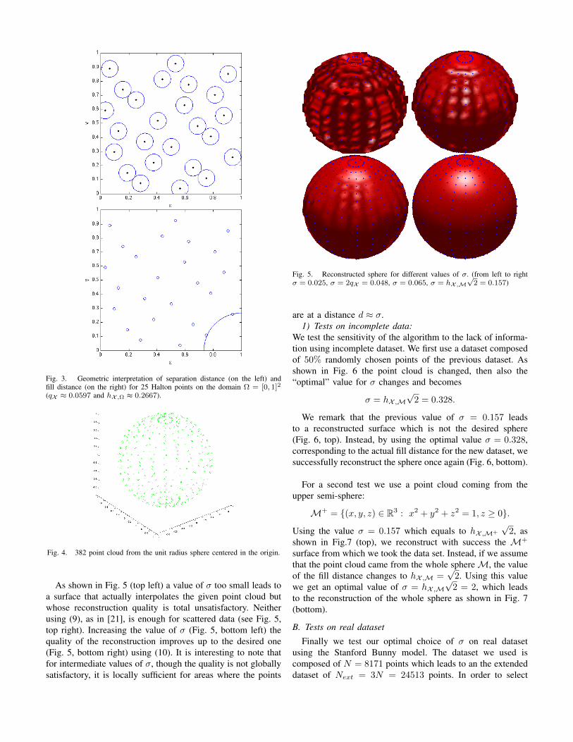
Fig. 3. Geometric interpretation of separation distance (on the left) andfill distance (on the right) for 25 Halton points on the domain Ω = [0, 1]2

(qX ≈ 0.0597 and hX ,Ω ≈ 0.2667).

Fig. 4. 382 point cloud from the unit radius sphere centered in the origin.

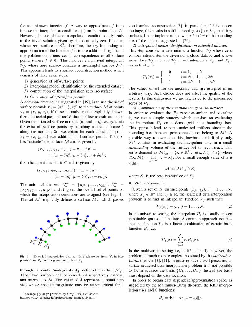
As shown in Fig. 5 (top left) a value of σ too small leads toa surface that actually interpolates the given point cloud butwhose reconstruction quality is total unsatisfactory. Neitherusing (9), as in [21], is enough for scattered data (see Fig. 5,top right). Increasing the value of σ (Fig. 5, bottom left) thequality of the reconstruction improves up to the desired one(Fig. 5, bottom right) using (10). It is interesting to note thatfor intermediate values of σ, though the quality is not globallysatisfactory, it is locally sufficient for areas where the points

Fig. 5. Reconstructed sphere for different values of σ. (from left to rightσ = 0.025, σ = 2qX = 0.048, σ = 0.065, σ = hX ,M

√2 = 0.157)

are at a distance d ≈ σ.1) Tests on incomplete data:

We test the sensitivity of the algorithm to the lack of informa-tion using incomplete dataset. We first use a dataset composedof 50% randomly chosen points of the previous dataset. Asshown in Fig. 6 the point cloud is changed, then also the“optimal” value for σ changes and becomes

σ = hX ,M√

2 = 0.328.

We remark that the previous value of σ = 0.157 leadsto a reconstructed surface which is not the desired sphere(Fig. 6, top). Instead, by using the optimal value σ = 0.328,corresponding to the actual fill distance for the new dataset, wesuccessfully reconstruct the sphere once again (Fig. 6, bottom).

For a second test we use a point cloud coming from theupper semi-sphere:

M+ = (x, y, z) ∈ R3 : x2 + y2 + z2 = 1, z ≥ 0.

Using the value σ = 0.157 which equals to hX ,M+

√2, as

shown in Fig.7 (top), we reconstruct with success the M+

surface from which we took the data set. Instead, if we assumethat the point cloud came from the whole sphereM, the valueof the fill distance changes to hX ,M =

√2. Using this value

we get an optimal value of σ = hX ,M√

2 = 2, which leadsto the reconstruction of the whole sphere as shown in Fig. 7(bottom).

B. Tests on real dataset

Finally we test our optimal choice of σ on real datasetusing the Stanford Bunny model. The dataset we used iscomposed of N = 8171 points which leads to an the extendeddataset of Next = 3N = 24513 points. In order to select

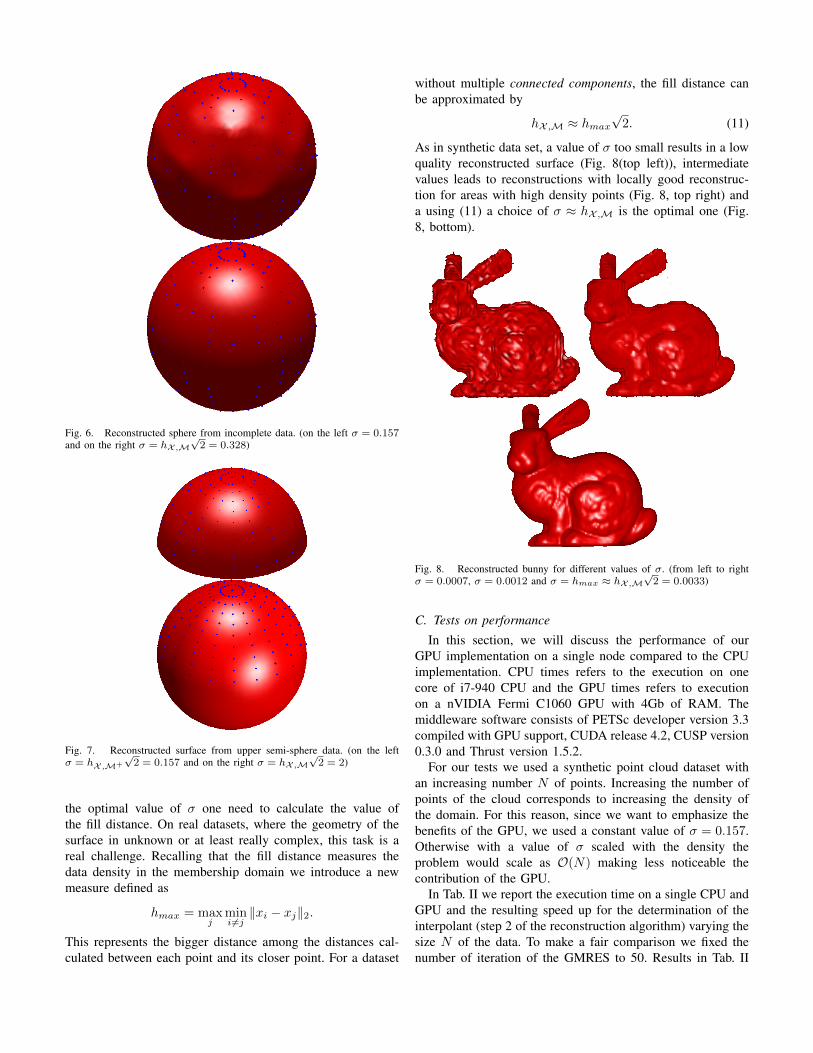
Fig. 6. Reconstructed sphere from incomplete data. (on the left σ = 0.157and on the right σ = hX ,M

√2 = 0.328)

Fig. 7. Reconstructed surface from upper semi-sphere data. (on the leftσ = hX ,M+

√2 = 0.157 and on the right σ = hX ,M

√2 = 2)

the optimal value of σ one need to calculate the value ofthe fill distance. On real datasets, where the geometry of thesurface in unknown or at least really complex, this task is areal challenge. Recalling that the fill distance measures thedata density in the membership domain we introduce a newmeasure defined as

hmax = maxj

mini 6=j‖xi − xj‖2.

This represents the bigger distance among the distances cal-culated between each point and its closer point. For a dataset

without multiple connected components, the fill distance canbe approximated by

hX ,M ≈ hmax√

2. (11)

As in synthetic data set, a value of σ too small results in a lowquality reconstructed surface (Fig. 8(top left)), intermediatevalues leads to reconstructions with locally good reconstruc-tion for areas with high density points (Fig. 8, top right) anda using (11) a choice of σ ≈ hX ,M is the optimal one (Fig.8, bottom).

Fig. 8. Reconstructed bunny for different values of σ. (from left to rightσ = 0.0007, σ = 0.0012 and σ = hmax ≈ hX ,M

√2 = 0.0033)

C. Tests on performance

In this section, we will discuss the performance of ourGPU implementation on a single node compared to the CPUimplementation. CPU times refers to the execution on onecore of i7-940 CPU and the GPU times refers to executionon a nVIDIA Fermi C1060 GPU with 4Gb of RAM. Themiddleware software consists of PETSc developer version 3.3compiled with GPU support, CUDA release 4.2, CUSP version0.3.0 and Thrust version 1.5.2.

For our tests we used a synthetic point cloud dataset withan increasing number N of points. Increasing the number ofpoints of the cloud corresponds to increasing the density ofthe domain. For this reason, since we want to emphasize thebenefits of the GPU, we used a constant value of σ = 0.157.Otherwise with a value of σ scaled with the density theproblem would scale as O(N) making less noticeable thecontribution of the GPU.

In Tab. II we report the execution time on a single CPU andGPU and the resulting speed up for the determination of theinterpolant (step 2 of the reconstruction algorithm) varying thesize N of the data. To make a fair comparison we fixed thenumber of iteration of the GMRES to 50. Results in Tab. II

shows that, even if the RASM preconditioner is not availablein CUSP, exploiting the GPU the execution time can be greatlydecreased.

TABLE IISPEED UP WITH GPU FOR INTERPOLANT DETERMINATION.

N CPU GPU Speed up1323 0,67551 0,1404 4,814686 34,567 5,6472 6,1215625 451,75 71,57 6,3124036 5398,4 815,09 6,63

In Tab. III are reported the execution time on CPU andGPU with the resulting speed up for the interpolant evaluation(step 3 of the surface reconstruction algorithm) varying thesize N of the point cloud and the size M of the evaluationgrid. As expected these execution time are substantially lowerthan those for the previous problem but in this case the GPUis fully exploited obtaining greater speed ups.

TABLE IIISPEED UP WITH GPU FOR EVALUATION OF INTERPOLANT.

M\N 1323 4686 15625 24036

15625CPU 0,11571 0,20605 0,78172 0,97539GPU 0,012831 0,033589 0,12167 0,13699

Speed up 9,01 6,13 6,42 7,12

125000CPU 0,60406 1,5657 5,9558 7,433GPU 0,029907 0,09974 0,32034 0,43697

Speed up 20,19 15,69 18,59 17,01

421875CPU 1,9098 5,2612 19,946 25,037GPU 0,084603 0,2892467 0,89695 1,1272

Speed up 22,57 18,18 22,23 22,211

1000000CPU 4,4389 12,505 47,594 59,501GPU 0,18456 0,60741 2,0629 2,4968

Speed up 24,05 20,58 23,07 23,83

1953125CPU 8,8515 24,431 92,589 116,39GPU 0,35668 1,0662 3,9195 4,8035

Speed up 24,81 22,91 23,62 24,23

3375000CPU 15,018 42,166 160,17 199,45GPU 0,59846 1,7525 6,4671 7,9468

Speed up 25,09 24,06 24,76 25,09

V. CONCLUSION

We have implemented a parallel implicit method basedon radial basis functions for surface reconstruction. Thisimplementation relies on parallel scientific libraries and issupported for the GPU device. Since the reconstruction qualityand the performances are strongly related to the gaussian RBFparameter σ, we propose an optimal and heuristic estimatebased on some density measures of the point cloud. Finally,the obtained speed-up and running time confirm that the RBFinterpolant can be a very effective algorithm for such problem.

REFERENCES

[1] Satish Balay, William Gropp, Lois Curfman McInnes, and Barry FSmith. Petsc, the Portable, Extensible Toolkit for scientific computation.Argonne National Laboratory, 2:17, 1998.

[2] R.K. Beatson, WA Light, and S. Billings. Fast solution of the radialbasis function interpolation equations: Domain decomposition methods.SIAM Journal on Scientific Computing, 22(5):1717–1740, 2001.

[3] Jonathan C Carr, Richard K Beatson, Jon B Cherrie, Tim J Mitchell,W Richard Fright, Bruce C McCallum, and Tim R Evans. Reconstruc-tion and representation of 3d objects with radial basis functions. InProceedings of the 28th annual conference on Computer graphics andinteractive techniques, pages 67–76. ACM, 2001.

[4] Jonathan C. Carr, W. Richard Fright, and Richard K Beatson. Surfaceinterpolation with radial basis functions for medical imaging. MedicalImaging, IEEE Transactions on, 16(1):96–107, 1997.

[5] P.C. Curtis. n-parameter families and best approximation. PacificJournal of Mathematics, 9(4):1013–1027, 1959.

[6] Cuomo, S. De Michele, P. Farina, R.Piccialli, F. A Smart GPUImplementation of an Elliptic Kernel for an Ocean Global CirculationModel, Applied Mathematical Sciences, Vol. 7, no. 61, 3007 - 3021(2013).

[7] R. Franke. Scattered data interpolation: Tests of some methods. Math.Comput., 38(157):181–200, 1982.

[8] Sarah F Frisken, Ronald N Perry, Alyn P Rockwood, and Thouis RJones. Adaptively sampled distance fields: a general representationof shape for computer graphics. In Proceedings of the 27th annualconference on Computer graphics and interactive techniques, pages249–254. ACM Press/Addison-Wesley Publishing Co., 2000.

[9] Jan Klein and Gabriel Zachmann. Point cloud surfaces using geometricproximity graphs. Computers & Graphics, 28(6):839–850, 2004.

[10] Marc Levoy, Kari Pulli, Brian Curless, Szymon Rusinkiewicz, DavidKoller, Lucas Pereira, Matt Ginzton, Sean Anderson, James Davis,Jeremy Ginsberg, Jonathan Shade, and Duane Fulk. The digitalmichelangelo project: 3d scanning of large statues. In Proceedingsof the 27th annual conference on Computer graphics and interactivetechniques, SIGGRAPH ’00, pages 131–144. ACM Press/Addison-Wesley Publishing Co., 2000.

[11] J.C. Mairhuber. On haar’s theorem concerning chebychev approxima-tion problems having unique solutions. Proceedings of the AmericanMathematical Society, pages 609–615, 1956.

[12] WR Madych and SA Nelson. Multivariate interpolation and condi-tionally positive definite functions. ii. Mathematics of Computation,54(189):211–230, 1990.

[13] Nathan Bell and Michael Garland. Cusp: Generic parallel algorithmsfor sparse matrix and graph computations, 2012. Version 0.3.0.

[14] Joachim Pouderoux, Jean-Christophe Gonzato, Ireneusz Tobor, andPascal Guitton. Adaptive hierarchical rbf interpolation for creatingsmooth digital elevation models. In Proceedings of the 12th annualACM international workshop on Geographic information systems, GIS’04, pages 232–240. ACM, 2004.

[15] Oliver Schall and Marie Samozino. Surface from scattered points. Ina Brief Survey of Recent Developments. 1st International Workshop onSemantic Virtual Environments, Page (s), pages 138–147, 2005.

[16] B. Smith, P. Bjorstad, and W. Gropp. Domain decomposition: parallelmultilevel methods for elliptic partial differential equations. CambridgeUniversity Press, 2004.

[17] J Sußmuth, Q Meyer, and G Greiner. Surface reconstruction basedon hierarchical floating radial basis functions. In Computer GraphicsForum, volume 29, pages 1854–1864. Wiley Online Library, 2010.

[18] Jared Hoberock and Nathan Bell. Thrust: A parallel template library,2010. Version 1.5.2.

[19] Greg Turk, Huong Quynh Dinh, James F O’Brien, and Gary Yngve.Implicit surfaces that interpolate. In Shape Modeling and Applications,SMI 2001 International Conference on., pages 62–71. IEEE, 2001.

[20] Greg Turk and James F O’brien. Variational implicit surfaces. 1999.[21] Rio Yokota, L.A. Barba, and Matthew G. Knepley. Petrbf a parallel o(n)

algorithm for radial basis function interpolation with gaussians. Com-puter Methods in Applied Mechanics and Engineering, 199(25):1793 –1804, 2010.

[22] H. Wendland. Scattered data approximation, volume 2. CambridgeUniversity Press Cambridge, 2005.

[23] Hong-Kai Zhao, Stanley Osher, and Ronald Fedkiw. Fast surfacereconstruction using the level set method. In Variational and LevelSet Methods in Computer Vision, 2001. Proceedings. IEEE Workshopon, pages 194–201. IEEE, 2001.