Surface Reflection ModelsFrank Losasso (flosasso@nvidia.com)

Introduction

One of the fundamental topics in lighting is how the light interacts with the environment.The academic community has researched several models over the last century, but for themost part, we are still stuck with the most basic of models. The reason for this is for themost part the lack of computational power, making it difficult to use more truthful modelsin real-time. The goal of this paper is to investigate the viability of some of the moresophisticated surface reflection models that have been created, giving developers a senseas to how much computational power needs to be used to create better looking surfaces.

Traditionally, the most used method of finding the color of a pixel has been throughGouraud interpolation of Lambert's Cosine Law at the vertices. This lighting model isextremely cheap to compute and is amenable to fixed function pipelines. With the adventof GPUs, Phong interpolation has become a viable option. This model has allowed forinnovations like bump mapping giving more realism to modern virtual worlds. Theunderlying assumptions however are still the same; the surfaces are Lambertian.Unfortunately, this has the side effect of making most of the computer generated imageslook very much alike, and very different from the real world. The Lambertian surfaceassumption works great for some materials (like plastic), which means that differentmodels must be used if other materials are to be represented faithfully. And this is whatwe will investigate over the next few pages.

The Lambertian Lighting Models

Lambert created this model over a century ago, and as mentioned previously, it is still themost used model (by a huge margin) in real time graphics today. Lambert assumed thatwhen light strikes a surface, the light is reflected equally in all directions. The light thatstrikes any given part of a surface is proportional to the cosine of the incident angle1.

The Lambertian Diffuse Lighting Equation:

LNfkkI attda

The cost of this equation is extremely small, and the results are usable, but it does givethe appearance that the lit object is made of rough plastic (no specular component).

1 Please see Appendix A for explanation of terms and symbols

Screenshot of Lambertian lighting

Diagram showing the amount of light emitted in all directions given a light direction (purple line)

The bottom two screenshots give a pictorial description of the behavior of the function.The white wireframe contour indicates how much light is given off in each direction, andthe purple line indicates the light vector (the direction from which the light is coming).Notice that when the light is coming from an angle, the amount of light reflected in alldirections is less that when the incident angle is close to zero (the light vector isperpendicular to the surface)

The Phong Lighting Model

Phong lighting is the other major lighting model that is used in real time rendering,especially after the advent of programmable pipelines. Phong did not change any ofLamberts assumptions, and hence the cosine of the angle between the incident lightvector and the surface normal is still used to calculate the diffuse component of thesurface. Phong did however create Phong interpolation that involves the interpolation ofthe vectors across the faces of the polygons as opposed to colors. The largest benefit ofinterpolating vectors across the polygon is that accurate specular highlights can be

reproduced. The major drawback of calculating the lighting equation at every pixel usingthese interpolated vectors is of course that a lot more computational power is used.

The Phong Lighting Equation:

nattsattda REfkLNfkkI )(

Two other advantages of Phong interpolation are that it is easy to add bump mapping tosurfaces, and the visual appearance of the surface is significantly better than per-vertexinterpolated lighting.

Objects that are lit by Phong lighting tend to look like various types of plastic (dependingon the specular exponent).

Screenshot of Phong lighting

Figures clearly showing that the specular highlight is in the direction of the reflection vector. Thediffuse component is the same as the Lambertian diffuse component.

The Cook-Torrance Lighting Model

The model presented by Cook and Torrance, strives for as much physical realism aspossible, as opposed to the models above that are made entirely ad-hoc for computergraphics only, the Cook-Torrance model uses physical properties, and has all the niceproperties one would expect a BRDF to have (such as energy conservation, complexsubstructures, and a predictive result).

BRDFs like Cook-Torrance also has the advantage of using parameters with physicalanalogies, meaning that artists can tweak the properties of the surface easily to createrealistic looking objects.

The Cook-Torrance model assumes that the surface is made up of microscopic perfectLambertian reflectors called microfacets. Several of the terms in the lighting equationdeal with how these microfacets are oriented, masked and shadowed.

The Cook-Torrance Lighting Equation

)(cos4

))(()(

)()()(

42

2)tan(

meD

NENLDGFfk

NEDGFkNLkkI

m

iatts

isda

The D term in the equation is the distribution function of the microfacets based on theBeckman distribution function. The m parameter is the root-mean-square (RMS) of theslope of the microfacets. This means that a large m makes the reflections spread out(since the average slope of the microfacets is larger). The G term is the geometricattenuation term, which deals with how the individual microfacets shadow and mask eachother. The F term is the Fresnel Conductance term that is wavelength dependent (noticethe ), but for computational simplicity, we will assume that it is wavelength independent(and hence only one calculation is needed). The Fresnel Conductance term deals with theamount of light that is reflected versus absorbed as the incident angle changes (anexample of this is often seen when driving on a straight road, and the road appearingmirror-like when viewed from grazing angles).

Screenshot of Cook-Torrance lighting

From these diagrams, it is clear that this BRDF is clearly different. Notice the complete change inbehavior when the incident angle is large

The Blinn Lighting Model

The Jim Blinn model for specular reflection is built on top of the work done in 1967 byTorrance and Sparrow who worked on a model to explain the fact that the specularintensity varies with both the direction of the light source and the direction of the viewer,whereas previous models had ignored the direction of the viewer. The Blinn Model is amodification of the Torrance-Sparrow model that yields similar results, but issignificantly cheaper to compute.

The Blinn Lighting Equation:

2

22

2

1)1()(

)()(

cHNcD

NEDGFfkI i

atts

The lighting equation has the same form as the Cook-Torrance lighting equation above,with a geometric attenuation factor and a Fresnel conductance term. The distributionfunction (D) is now significantly easier to compute.

Screenshot of Blinn lighting

Diagrams depicting the Blinn BRDF clearly show that Blinn lighting is similar to Cook-TorranceLighting

It is evident from the screenshots that it is now possible to make surfaces that look morelike metal than plastic using this equation, but without the huge cost of the Cook-Torrance or the Torrance-Sparrow models. Just like all the other per pixel based methods,the per pixel version of this lighting model is also amenable to add-ons such as bumpmapping.

The Oren-Nayar Lighting Model

Oren and Nayar created a new BRDF in the hope to ‘generalize’ the Lambertian diffuselighting model. This BRDF can reproduce several rough surfaces very well, including

wall plaster, sand, sand paper, clay, and others. It is however very computationallyexpensive, and it requires the calculation of azimuth and zenith angles.

The need for a better diffuse lighting model seems very real, and in their original paper,Oren and Nayar presented a clay vase that was rendered using the Lambertian and theirproposed models compared to a real image. It is glaringly obvious from thatdemonstration that the Lambertian model was not suitable for representing certainmaterials, whereas in this case their model was much better.

This lighting equation can be calculated either per-pixel or per-vertex, and a per-pixelimplementation is amenable to bump mapping, although the pixel program may getprohibitively expensive.

The Oren-Nayar Lighting Equation (the simplified qualitative model):

09.045.0

33.05.00.1

)tan()sin()cos(,0max)cos(

2

2

2

2

0

B

A

BAEfkI iriattd

The lighting equation above is simplified model that Oren and Nayar presented in theirpaper. It ignores terms like inter-reflections, in an effort to make the model cheaper tocalculate.

Since hardware like nv30 can calculate the above equation in hardware, at the fragmentshader level, no preprocessing is necessary, which is helpful if the light configuration orthe geometry is modified.

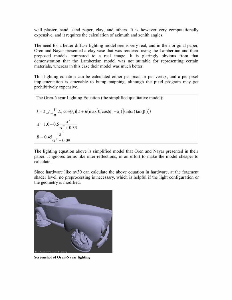
Screenshot of Oren-Nayar lighting

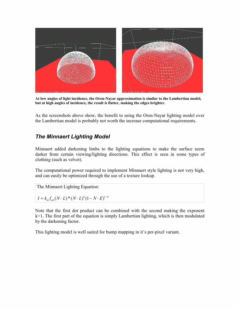
At low angles of light incidence, the Oren-Nayar approximation is similar to the Lambertian model,but at high angles of incidence, the result is flatter, making the edges brighter.

As the screenshots above show, the benefit to using the Oren-Nayar lighting model overthe Lambertian model is probably not worth the increase computational requirements.

The Minnaert Lighting Model

Minnaert added darkening limbs to the lighting equations to make the surface seemdarker from certain viewing/lighting directions. This effect is seen in some types ofclothing (such as velvet).

The computational power required to implement Minnaert style lighting is not very high,and can easily be optimized through the use of a texture lookup.

The Minnaert Lighting Equation:

kkattd ENLNLNfkI 1)1()(*)(

Note that the first dot product can be combined with the second making the exponentk+1. The first part of the equation is simply Lambertian lighting, which is then modulatedby the darkening factor.

This lighting model is well suited for bump mapping in it’s per-pixel variant.

Screenshot of Minnaert lighting

It is clear from the diagrams that the darkening limbs bring the amount of light reflected towardszero when the viewer looks onto the surface at perpendicular angles

Wards Anisotropic Lighting Model

An isotropic surface has the property that for any given point on the surface, the lightreflected does not change when the surface is rotated about the normal. This is the casefor many materials, but some materials such as brushed metal or hair this is not the case.The reason for these anisotropic surfaces is that the micro facets that make up the surfacehave a preferred direction in the form of parallel grooves or scratches. There are severalad-hoc models for lighting anisotropic surfaces that have been developed for use in realtime graphics. Other nVidia demos for anisotropic lighting use a texture lookup based onthe cosine of the angle between the surface normal and the light vector one axis, and thecosine of the angle between the surface normal and the half angle vector on the other axis.If the texture map has a bright line down the diagonal, then the surface will be brightwhen those two values are approximately the same. The approach presented here does notuse any textures, but is instead based on the BRDF introduced by Greg Ward Larson in1992.

The Ward Anisotropic Reflection Model:

)(12

22

4)(

))((1)( NH

YHXH

yxattsattd

yx

eLNENLN

fkLNfkI

The X and Y terms are two perpendicular tangent directions on the surface. They giverepresent the direction of the grooves in the surface. The terms are the standarddeviations of the slope in the X and Y direction (given by their respective subscripts).

Proper tessellation is essential when per vertex calculations are used; otherwise per pixelcalculations should be used.

Screenshot of Wards Anisotropic lighting (The grooves in the surface were made to look like circularbrushed metal patterns)

The diagrams of the function clearly show that the lobe of reflected light is oriented perpendicularlyto the groove in the surface (the grove is oriented with the wireframe box in the left-right direction)

Environment Mapping Based Lighting Models

A lot of research has been done recently on environment map based lighting. Mosttechniques are concerned with different ways of creating the environment map, to create arealistic looking lighting model. The nice things about environment maps is that it’s allprecomputed and as long as the lights are static, and the surface being lit doesn’t changeposition too much, environment mapping is a very good looking, and very cheap way oflighting objects.

The general idea of environment map based lighting is that all of the lightingcomputations are done off-line for all directions at a given point, P. The data is thenstored in a cube map, which is used to fetch the light value for any point on a surface thatis approximately located where the original point P was. This means that incrediblycomplex and expensive lighting solutions can be computed, and then cheaply applied toan object in real-time when required.

There are several drawbacks to the method as well, many of which should be apparentfrom the paragraph above. If the surface being lit is not at the location where the point Pwas, then the cube map may be useless, and creating a new one may be prohibitivelyexpensive. If any of the lights lighting the scene are moved, then the cube map will alsohave to be computed, so in general, the technique is only great for a complex object thatis relatively far away from static lights in comparison to it’s size and the movements itwill make.

Appendix A

The following table gives each symbol used in this paper and an explanation.

Symbol Name ExplanationI Intensity The output intensity from the lighting equation. This is

the final intensity of the fragment.kd Diffuse Reflection

CoefficientThe fraction of light that is reflected through diffusereflection

ks Specular ReflectionCoefficient

The fraction of light that is reflected through specularreflection (note that the diffuse and specular coefficientsshould add up to one)

N Surface Normal Normalized direction vector that is perpendicular to thesurface

L Light Vector Normalized direction vector that points from the surfacepoint to the light location

E Eye Vector Normalized direction vector that points from the surfaceto the viewer (camera location)

H Half Vector Normalized direction vector that is the average of thelight and viewing vector (normalize (L+V))

R Reflection Vector Normalized vector that is in the direction of the LightVector, rotated around the Normal Vector 180 degrees.Calculated as follows:

LNNLR )(2n Specular Exponent The specular exponent determines how ‘sharp’ the

specular highlight is (higher is ‘sharper’)c Ellipsoid

EccentricityThe eccentricity of the micro facets (0 for very shiny, 1for very dull)

c1,c2,c3 AttenuationCoefficients

The coefficients for constant, linear and quadraticattenuation of the light source, respectively.

d Light Distance The distance to the lightG Geometric

AttenuationThe attenuation factor due to self-shadowing andmasking of micro facets on the surface. Calculated asfollows:

HV

LNHNHE

ENHNG ))((2,))((2,1min

F FresnelConductance Term

Fresnel determines the amount of reflection of thesurface (increases as the zenith angle becomes larger).Calculated as follows:

1

)cos()1)(()1)((1

)()(

21

22

2

2

2

2

cng

HLccgccgc

cgcgF

i

For simplification, the Fresnel conductance term canalso be a approximated by the following (much cheaper)equation:

55 )(1)(11 ENnENF fatt Attenuation Term The fraction of light that reaches the surface as an effect

of light attenuation. Calculated as follows:

)1,1min(2

321 dcdccf att

Note that is real life, light is attenuated with the squareof the distance, but often, the heuristic (hack) aboveworks better.

Appendix B

The following table shows the relative costs of the different lighting models in terms ofvertex shaders, pixel shaders, and texture lookups.

0

20

40

60

80

100

120

140

160

Lambert

ian (p

er ve

rtex)

Lambert

ian (p

er pix

el)

Phong

Cook-T

orran

ce (p

er vert

ex)

Cook-T

orran

ce (p

er pixe

l)

Blinn (

per v

ertex

)

Blinn (

per p

ixel)

Oren-N

ayar

(per v

ertex

)

Oren-N

ayar

(per p

ixel)

Minnae

rt (pe

r vert

ex)

Minnae

rt (pe

r pixe

l)

Anisotro

pic (pe

r vert

ex)

Anisotro

pic (pe

r pixe

l)

Enviro

nmen

tal (p

er ve

rtex)

Pixel Shader Cost

Vertex Shader Cost

Lamberti

an(pervertex)

Lamberti

an(perpixe

l)Pho

ng

Cook-

Torranc

e(pervertex)

Cook-

Torranc

e(perpixe

l)

Blinn

(pervertex)

Blinn

(perpixe

l)

Oren-

Nayar

(pervertex)

Oren-

Nayar

(perpixe

l)

Minnaer

t(pervertex)

Minnaer

t(perpixe

l)

Anisotropic

(pervertex)

Anisotropic

(perpixe

l)

Environ

mental

(pervertex)

Vertex Shader Cost 32 27 29 106 28 79 28 83 28 57 28 108 28 32Pixel Shader Cost x 31 51 x 109 x 80 x 88 x 50 x 103 xTextures Required 0 0 0 0 0 0 0 0 0 0 0 0 0 1+